on the stop-loss and total variation distances between random sums

Statistics & Probability Letters 53 (2001) 153–165

On the stop-loss and total variation distances betweenrandom sums

Michel Denuit ∗, S&ebastien Van BellegemInstitut de Statistique, Universit�e Catholique de Louvain, Voie du Roman Pays, 20, B-1348 Louvain-la-Neuve, Belgium

Received October 2000; received in revised form March 2001

Abstract

The purpose of this work is to provide upper bounds on the stop-loss and total variation distances between randomsums. The main theoretical argument consists in de0ning discrete analogs of the classical ideal metrics considered byRachev and R1uschendorf (Adv. Appl. Probab. 22 (1990) 350). An application in risk theory enhances the relevance ofthe approach proposed in this paper. c© 2001 Elsevier Science B.V. All rights reserved

Keywords: Probability metrics; Stop-loss distances; Total variation distances; Random sums; s-convex orderings; Risktheory

1. Introduction and Motivation

In this paper, we are interested in the stop-loss and total variation probability metrics that can be found inRachev and R1uschendorf (1990). The latter map a couple of distribution functions to the extended half-positivereal line 7R+ and possess the metric properties of symmetry, triangle inequality and a suitable analog of theidenti0cation property. The use of metrics in many problems of applied probability allows one to decidewhether the proposed stochastic model provides a satisfactory approximation to the real model, and if so,within what limit. Recently, metrics have received considerable interest in probability theory and mathematicalstatistics. For a thorough presentation of probability metrics, we refer the interested reader e.g. to Rachev(1991).The metrics now used in applied probability number in the dozens. Let us recall the de0nition of several

classical distances that we will consider in this paper. First, the total-variation distance dTV between twonon-negative random variables X and Y with respective distribution functions FX and FY is given by

dTV(X; Y ) =∫t∈R+

|dFX (t)− dFY (t)|;

∗ Corresponding author. Tel.: +32-10-47-28-35; fax: +32-10-47-30-32.E-mail addresses: [email protected] (M. Denuit), [email protected] (S. Van Bellegem).

0167-7152/01/$ - see front matter c© 2001 Elsevier Science B.V. All rights reservedPII: S0167 -7152(01)00067 -0

154 M. Denuit, S. Van Bellegem / Statistics & Probability Letters 53 (2001) 153–165

the latter de0nition slightly diEers from the standard one (by a constant factor, in fact) for reasons whichwill later become obvious to the reader. It is worth mentioning that we write by abuse of notation dTV(X; Y )whereas dTV(FX ; FY ) would be more appropriate since dTV does not depend on the particular versions of therandom variables X and Y (i.e., dTV, as all the other metrics considered in this paper, is a simple metric).Another popular metric is the Kolmogorov (or uniform) metric dK, de0ned as

dK(X; Y ) = supt∈R+

|FX (t)− FY (t)|:

The de0nition of dK is based on the famous Kolmogorov–Smirnov test statistic. The Wasserstein distance,also known as the Dudley or Kantorovitch distance, is de0ned as

dW(X; Y ) =∫t∈R+

|FX (t)− FY (t)| dt:

In actuarial sciences, Gerber (1981) de0ned the stop-loss distance as

dsl(X; Y ) = supt∈R+

|E(X − t)+ − E(Y − t)+|;

where x+ = max{x; 0}. The metric dsl has been used e.g. by Gerber (1981, 1984), and De Pril and Dhaene(1992). In addition to the distances recalled above, we also consider the classes of the stop-loss and total-variation distances that can be found in Rachev and R1uschendorf (1990).The problem examined in the present paper can be described as follows. Let d be a probability distance.

Given the sequences {X1; X2; X3; : : :} and {Y1; Y2; Y3; : : :} of independent and identically distributed non-negativerandom variables, and two counting random variables N and M independent of the Xi’s and of the Yi’s,respectively, let us de0ne the compound sums

SN =N∑k=1

Xk; SM =M∑k=1

Xk and TM =M∑k=1

Yk (1.1)

with the convention that the empty sum equals 0. Considering non-negative integer-valued summands, Vel-laisamy and Chaudhuri (1996) have shown in their Lemma 3:1 that

dTV(SN ; SM )6 dTV(N;M) (1.2)

in the special case of Bernoulli summands, (1.2) has been obtained by Finkelstein et al. (1990, Lemma 4).Vellaisamy and Chaudhuri (1996) also proved that

dTV(SN ; TM )6 dTV(N;M) + min{EM; EN}dTV(X1; Y1) (1.3)

see their Theorem 3:1. One of the aim of this paper is to generalize the inequalities (1.2) and (1.3) to dK,dW and dsl, as well as to the whole classes of stop-loss distances and total-variation distances. Moreover, wedo no more assume that the summands Xi and Yi are integer-valued but we deal with the general situation ofnon-negative random variables.Our main theoretical vehicle are discrete distances, suitable to evaluate the closeness of counting random

variables; these discrete counterparts of the stop-loss and total variation distances have been de0ned in Denuitet al. (2000) and have proved their usefulness in various problems encountered in actuarial risk theory.In the building of appropriate stochastic models, it is often interesting to be able to compare random

variables relating to the diEerent models. To this end, one usually resorts to stochastic orderings, i.e. to binaryrelations de0ned on sets of distribution functions. These relations aim to mathematically translate intuitiveideas as “being larger”, or “being more variable”, for instance. For a comprehensive background on stochasticorderings including a variety of applications, the reader is referred, e.g. to Shaked and Shanthikumar (1994). Inthis paper, we will be interested in classes of integral stochastic orderings; such orderings are de0ned with thehelp of classes of measurable functions using the operator expectation. Speci0cally, considering two random

M. Denuit, S. Van Bellegem / Statistics & Probability Letters 53 (2001) 153–165 155

variables X and Y; X is said to be smaller than Y in the integral stochastic order ≺F generated by the classF of measurable functions if, E�(X )6 E�(Y ) for all functions � ∈ F, provided that the expectations exist.A general study of these orderings is made in M1uller (1997). Taking for F the class of the non-decreasingfunctions yields the stochastic dominance 4st. Similarly, if F is the class of the (non-decreasing) convexfunctions then 4F is the (increasing) convex order 4(i)cx.Traditionally, these orderings are de0ned for random variables X and Y which take on values in R or R+ (or

an entire interval). Orderings proper to discrete random variables X and Y have received much less attention.The basic situation is when all outcomes lie in the set N of the non-negative integers. In this framework, theclasses F represent classes of functions de0ned only on N and, roughly, as in the continuous case but withthe operator of forward diEerence substituted for the operator of derivative. We refer the interested reader,e.g. to Fishburn and Lavalle (1995), LefLevre and Utev (1996), Denuit and LefLevre (1997) and Denuit et al.(1999) for more details.A crucial point, which has often been ignored in the literature, is the close link existing between probability

metrics and stochastic orderings. In that respect, we expand here on the pioneering work of LefLevre and Utev(1998), who were the 0rst authors to systematically exploit the relationships between metrics and orderingsgenerated by classes of measurable functions.Henceforth, we con0ne our analysis to non-negative random variables. Given a random variable X , FX

denotes the cumulative distribution function (cdf, in short) of X , i.e. FX (t)=P[X 6 t], t ∈ R, and 7FX ≡ 1−FXdenotes the decumulative distribution function (ddf, in short) or survival function of X , i.e. 7FX (t)=P[X ¿ t],t ∈ R. The probability density function (pdf, in short) of X with respect to some dominating measure(Lebesgue measure on the half-positive real line R+ or counting measure on the non-negative integers N) isdenoted as fX . We use capital letters X; Y; Z; : : : to represent continuous random variables and capital lettersM;N;O; : : : to represent integer-valued random variables.To end this introduction, let us say a few words about the organization of the present paper. Denuit et al.

(1998) showed how to generalize the standard stochastic dominance, convex and increasing convex orders togeneral classes of integral stochastic orderings called s-convex and s-increasing convex orders; we brieQy recallthis construction in Section 2. A similar generalization is possible in the spirit of Rachev and R1uschendorf(1990) for dTV, dK, dW and dsl; this will be done in Section 3. Under appropriate ordering conditions,distances between random variables reduce to diEerences of moments. In both Sections 2 and 3, we stress thesimilarities and complementarities between discrete and continuous orderings=distances. In Section 4, upperbounds for various distances between random sums are derived extending (1.2) and (1.3). The key technicalargument is the discrete version of the probabilistic distances introduced in Section 3. Finally, Section 5 givesan application in risk theory which enhances the relevance of the approach developed in the present paper.

2. Stochastic orderings of convex-type

2.1. Comparing continuous random variables

2.1.1. Continuous iterated right-tailsLet X be a random variable valued in R+ with pdf fX . To X is associated the sequence { 7F [k]X ; k=1; 2; 3; : : :}

of its iterated right-tails obtained by repeated integration of the pdf over regions (t;+∞). Speci0cally, the7F[k]X ’s are de0ned recursively as follows:

7F[0]X ≡ fX and 7F

[k+1]X (t) =

∫ +∞

x=t

7F[k]X (x) dx; t ∈ R+: (2.1)

Note in passing that 7F[1]X coincides with the ddf 7FX of X ; 7F

[k]X is referred to as the kth iterated right-tail of

X . Iterated right-tail functions are closely related to the stop-loss transforms or partial moments. Speci0cally,


it can be shown by induction and successive applications of Fubini’s theorem that

(s− 1)! 7F [s]X (t) = E(X − t)s−1+ ; t ∈ R+ (2.2)

with the convention that (x − t)0+ = 1 if x¿ t and 0 otherwise. The name “stop-loss” transform comes from

the fact that 7F[2]X (t) = E(X − t)+ is called the stop-loss premium with deductible t in risk theory.

2.1.2. Continuous orderings of convex-typeMany comparisons of random variables X and Y are based on the iterated right-tails, as those introduced

by Denuit et al. (1998) whose de0nition is recalled next. Given two non-negative random variables X and Ywith 0nite moments of degree s− 1, X is said to precede Y in the s-convex sense, denoted as X 4R+

s Y , ifEX k = EY k for k = 1; 2; : : : ; s − 1 and 7F

[s]X (t) 6 7F

[s]Y (t) for all t ∈ R+. As particular cases of the stochastic

orderings 4R+s , 4

R+1 is the usual stochastic dominance 4st, while 4R+

2 coincides with the well-known convexorder 4cx.

2.2. Comparing discrete random variables

2.2.1. Discrete iterated right-tailsLet us de0ne for arithmetic random variables the analogs of the continuous iterated right-tails de0ned in

(2.1). Let N be a random variable valued in N. To N is associated the sequence { 7F [k]N ; k = 1; 2; : : :} of itsiterated right-tails obtained by repeated summation of the pdf over regions { j; j + 1; j + 2; : : :}. Speci0cally,the 7F

[k]N ’s are de0ned recursively as follows:

7F[0]N ≡ fN and 7F

[k+1]N (j) =

+∞∑i=j

7F[k]N (i); j ∈ N: (2.3)

It is interesting to compare (2.1) and (2.3). It is worth mentioning that we do not formally adopt a diEerentnotation for the discrete iterated right-tails 7F

[k]N and the continuous ones 7F

[k]X ; the context will make clear

which integrated right-tails are used.Of course, the reader familiar with measure theory has rapidly discovered that a general de0nition of iterated

right-tails calling upon dominating measures could easily be developed. However, we will not follow this routehere and con0ne ourselves to the standard continuous and discrete cases, which appear to be suTcient for theapplications we have in mind.LefLevre and Utev (1996) proved that the 7F

[s]N ’s correspond to some factorial moments speci0cally, for any

j; k ∈ N, the equalities

7F[s]N (j) = E

(N − j + s− 1

s− 1)=

1(s− 1)!E [(N − j + s− 1) : : : (N − j + 1)] (2.4)

hold true, with the convention that ( �1�2 ) = 0 if �1¡�2. Again, compare (2.2) to (2.4).

2.2.2. Discrete orderings of convex-typeDenuit and LefLevre (1997) de0ned the s-convex stochastic orderings among integer-valued random variables

as follows. Let N and M be two random variables valued in N, N is said to precede M in the s-convexsense, written as N 4N

s M , if ENk = EMk for k = 1; : : : ; s− 1, and 7F

[s]N (j)6 7F

[s]M (j) for all j ∈ N.


The orderings 4Ns and 4

R+s are not equivalent for s¿ 3, whereas they coincide for s= 1; 2, as shown by

Denuit, et al. (1999). More speci0cally, given two integer-valued random variables N and M , we have that

N 4N1 M ⇔ N 4R+

1 M ⇔ N 4st M

N 4N2 M ⇔ N 4R+

2 M ⇔ N 4cx M

and

N 4Ns M ⇒ N 4R+

s M for s¿ 3

with a generally false reciprocal. From the three latter relations, we see that a ranking in the 4Ns -sense for

counting random variables is more informative as soon as s¿ 3.

3. Metrics of convex-type

3.1. Distances between continuous random variables

Rachev and R1uschendorf (1990) introduced useful distances based on iterated right-tails; these authors applythem to measure the closeness between the individual and the collective models in risk theory. We resort hereon a slight modi0cation of their de0nition.

De�nition 3.1. (i) Given two random variables X and Y valued in R+, the stop-loss distance of degree sbetween X and Y , denoted as dR

+

s (X; Y ), is de0ned by

dR+

s (X; Y ) = supt∈R+

| 7F [s]X (t)− 7F[s]Y (t)|;

where 7F[s]X and 7F

[s]Y are de0ned according to (2.1).

(ii) Given two random variables X and Y valued in R+, the total variation distance of degree s betweenX and Y , denoted as DR

+

s (X; Y ), is de0ned as

DR+

s (X; Y ) =∫t∈R+

| 7F [s]X (t)− 7F[s]Y (t)| dt;

where 7F[s]X and 7F

[s]Y are de0ned according to (2.1).

The main diEerence between our De0nition 3.1 and Rachev and R1uschendorf, (1990) study is that we de0nedR

+

s by a supremum over t ∈ R+ rather than over t ∈ R. This modi0cation enables us to measure the distancebetween random variables with diEerent moments. For instance, the distance between two negative exponentialdistributions is easily computed with our de0nition and reduces up to a constant factor to the diEerence of the(s − 1)th moments for s ¿ 2 whereas this distance is in0nite for s ¿ 2 in Rachev and R1uschendorf (1990)framework. Considering the introduction, we have dR

+

1 (X; Y ) = dK(X; Y ) and dR+2 (X; Y ) = dsl(X; Y ).

The metric DR+

s is closely related to the Zolotarev metric �s (denoted as ds;1 in Rachev and R1uschendorf,1990); it can be shown that they are equivalent provided X and Y have identical 0rst s − 1 moments.Nevertheless, DR

+

s can be used to measure the distance between two random variables with diEerent 0rstmoments, whereas �s is in0nite in such a case. Considering the introduction, we have DR

+

0 (X; Y ) = dTV(X; Y )and DR

+

1 (X; Y ) = dW(X; Y ).


3.2. Distances between discrete-random variables

The discrete analogs of dR+

s and DR+

s have been introduced by Denuit et al. (2000). As it was the casefor stochastic orderings, the construction of the discrete versions of the stop-loss and total variation metricsis similar to their continuous counterparts, substituting the discrete iterated right-tails for the continuous ones.

De�nition 3.2. (i) Given the random variables N and M valued in N, the stop-loss distance of degree sbetween N and M , denoted as dNs (N;M), is de0ned as

dNs (N;M) = supj∈N

| 7F [s]N (j)− 7F[s]M (j)|;

where 7F[s]N and 7F

[s]M are de0ned according to (2.3).

(ii) Given the random variables N and M valued in N, the total variation distance of degree s between Nand M , denoted as DNs (N;M), is de0ned as

DNs (N;M) =+∞∑j=0

| 7F [s]N (j)− 7F[s]M (j)|;

where 7F[s]N and 7F

[s]M are de0ned according to (2.3).

Given two integer-valued random variables N and M , we can obviously resort on dR+

s and dNs to asserttheir respective distance. As a matter of fact, if s is equal to 1 or 2, it is equivalent measure their closenesswith the help of the discrete or the continuous stop-loss distances. A similar result holds for total variationdistances. More precisely, we have the following property.

Proposition 3.3. Given two random variables N and M valued in N, we have dNs (N;M) = dR+s (N;M) for

s= 1 or 2. Similarly, DNs (N;M) = DR+s (N;M) for s= 0 or 1.

Proof. The equality dN1 (N;M) = dR+1 (N;M) is obvious. Let us now turn to s= 2. Since

E(N − j + 1

1

)= Emax{N − j + 1; 1}= 1 + E(N − j)+

the stop-loss distance is equivalently given by

dN2 (N;M) = supj∈N

|E(N − j)+ − E(M − j)+|:

Now, for k 6 t ¡ k + 1, it is easily seen that the formula

E(N − t)+ = E(N − k)+ + (t − k) 7FN (k)holds true. Therefore, denoting as [t] the integer part of the real number t, we have

dR+

2 (N;M) = supt∈R+

|E(N − t)+ − E(M − t)+|

= supt∈R+

|E(N − [t])+ − E(M − [t])+ + (t − [t]){ 7FN ([t])− 7FM ([t])}|

= dN2 (M;N )

as announced. By the same argument, a similar result holds when we consider the total variation distance ofdegree s= 0 or 1.


Considering Property 3:3, we see that the discrete and continuous versions of the standard distances dTV,dK, dW and dsl coincide. However, this is no more necessarily true for higher degrees stop-loss and totalvariation metrics, as pointed out in Denuit et al. (2000). More precisely, given two random variables N andM valued in N, we only have

dR+

s (N;M)6 dNs (N;M) for s¿ 3: (3.1)

As we will see in the following result, this inequality may be strict in some general cases. In other words,considering arithmetic random variables as continuous ones underestimates the distance existing between them.Intuitively speaking, the arithmetic random variables N and M look more similar if we consider the set ofall the non-negative random variables (because they have the discreteness property in common) than if werestrict ourselves to random variables valued in N. Let us now provide a suTcient condition to have a strictinequality in (3.1).

Proposition 3.4. Let N and M be two random variables valued in N and let an integer s ¿ 3 be given.If the stochastic inequality N 4N

p M strictly holds for some p¡s − 1 (i.e. N and M are not identicallydistributed) then we have a strict inequality in (3.1).

Proof. First, we note that the 4Np ranking implies that

7F[k]N (t)6 7F

[k]M (t) for all t ∈ R+and any k ¿ p+ 1:

By diEerentiation, we see that the supremum de0ning dR+

s is attained for t = 0 so that

dR+

s (N;M) =EMs−1 − ENs−1

(s− 1)! :

Secondly, the 4Np ranking also yields

7F[k]N (j)6 7F

[k]M (j) for all j ∈ N and k ¿ p+ 1:

Therefore, the supremum de0ning dNs is attained for j = 0 and

dNs (N;M) =1

(s− 1)!

EMs−1 − ENs−1 +

s−2∑k=p

�k(EMk − ENk) ;

where �k are the coeTcients of the Newton expansion which are non-negative. It 0nally follows that dNs (N;M)¿dR

+

s (N;M), as announced.

The condition given in Property 3:4 is general enough. One may take for instance for N and M two Poissondistributed random variables with EN ¡ EM . In this case, the condition is ful0lled with p= 1.A similar result holds for the total variation distance. In this case, we have for any two random variables

N and M valued in N that

DR+

s (N;M)6 DNs (N;M) for s¿ 2: (3.2)

The counterpart of Property 3:4 for total variation distances is stated next. Since the proof follows the samelines than the reasoning developed in Property 3:4, we omitted it for brievety.

Proposition 3.5. Let N and M be two random variables valued in N and let an integer s¿ 2 be given. If thestochastic inequality N 4N

p M strictly holds for some p¡s (i.e. N and M are not identically distributed)then we have a strict inequality in (3.2).


Let us now show that the use of dR+

s in lieu of dNs may yield diEerent conclusions. Indeed, there existssome random variables N; M and O valued in N such that dNs (N;M)¡d

Ns (N;O) but d

R+s (N;M)¿d

R+s (N;O).

In such a case, we conclude on the basis of dNs that M is closer to N than O but resorting on dR+

s yields theopposite conclusion.For simplicity, we will show an example for s = 3. Let N be Poisson distributed with parameter �1, O

conforms to the Poisson distribution with parameter �2 and M obeys to a mixture of Poisson laws with randomparameter such that E = �1 and �22 + �2− �21¡ E 2¡�2 + �22− �21 + 3 (�2 − �1) (take for example �1 = 1and �2 = 2). For these variables, it is easy to see that

dR+

3 (N;O) =12 (�

22 − �21 + �2 − �1)

¡dR+

3 (N;M) = dN3 (N;M) =

12(E 2 − �1)

¡dN3 (N;O) =12(�22 − �21 + �2 − �1) + 3(�2 − �1):

4. Analysis of random sums

The metrics DR+

s and dR+

s are both ideal; as a consequence, the inequalities dR+

s (Sn; Tn)6 ndR+

s (X1; Y1) andDR

+

s (Sn; Tn)6 nDR+

s (X1; Y1) both hold true. Ideal probabilistic distances are appropriate to deal with variousapproximation problems involving sums of random variables (see e.g. Rachev, 1991, Chapter 14). A straightextension of this result consists in replacing the deterministic number of terms n by a couting random variableN independent of the Xi’s and of the Yi’s. This results in

dR+

s (SN ; TN )6 ENdR+

s (X1; Y1) and DR+

s (SN ; TN )6 ENDR+

s (X1; Y1):

However, the derivation of an upper bound on dR+

s (SN ; TM ) seems to be an open problem. This is due to thelack of the discrete counterpart dNs of d

R+s . Partial solutions have been proposed in the literature for dTV, e.g.

by Finkelstein et al. (1990) who considered in their Lemma 4 compound sums of Bernoulli random variablesand by Vellaisamy and Chaudhuri (1996) who considered in their Lemma 3:1 integer-valued summands. Inthis section, we aim to bound the distances DR

+

s and dR+

s between two compound sums SN and TM .Before stating our main result, we need the following technical lemma.

Lemma 4.1. Let " denote the classical forward di9erence operator, i.e. given a function � : N → R,"�(n) = �(n+ 1)− �(n), n ∈ N. Further, let "s denote the sth iterated of " (with the convention that "0

is the identity). We have that "sE[Ssn] = s!(EX1)s.

Proof. The announced result is true for s = 1 since "E[Sn] = E[Sn+1 − Sn] = EX1. Let us now proceed byinduction: we assume that "kE[Skn ]= k!(EX1)k is valid for any k 6 s− 1, and we aim to establish the desiredresult for s. Let us start from

"sESsn = E"sSsn = E"s(Ss−1n Sn)

= Es∑j=0

(sj

)"jSs−1n "s−jSn+j

which follows from the Leibniz formula for forward diEerences. Now, with the aid of the Newton formula,it is not diTcult to check that

"s−jSn+j =s−j∑l=0

(s− jl

)(−1)s−j−l(Xn+j+1 + · · ·+ Xn+j+l)


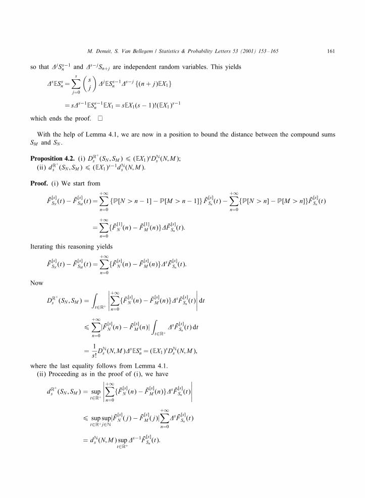
so that "jSs−1n and "s−jSn+j are independent random variables. This yields

"sESsn =s∑j=0

(sj

)"jESs−1n "s−j {(n+ j)EX1}

= s"s−1ESs−1n EX1 = sEX1(s− 1)!(EX1)s−1

which ends the proof.

With the help of Lemma 4.1, we are now in a position to bound the distance between the compound sumsSM and SN .

Proposition 4.2. (i) DR+

s (SN ; SM )6 (EX1)sDNs (N;M);(ii) dR

+

s (SN ; SM )6 (EX1)s−1dNs (N;M).

Proof. (i) We start from

7F[s]SN (t)− 7F

[s]SM (t) =

+∞∑n=0

{P[N ¿n− 1]− P[M ¿n− 1]} 7F [s]Sn (t)−+∞∑n=0

{P[N ¿n]− P[M ¿n]} 7F [s]Sn (t)

=+∞∑n=0

{ 7F [1]N (n)− 7F[1]M (n)}" 7F [s]Sn (t):

Iterating this reasoning yields

7F[s]SN (t)− 7F

[s]SM (t) =

+∞∑n=0

{ 7F [s]N (n)− 7F[s]M (n)}"s 7F [s]Sn (t):

Now

DR+

s (SN ; SM ) =∫t∈R+

∣∣∣∣∣+∞∑n=0

{ 7F [s]N (n)− 7F[s]M (n)}"s 7F [s]Sn (t)

∣∣∣∣∣ dt

6+∞∑n=0

| 7F [s]N (n)− 7F[s]M (n)|

∫t∈R+

"s 7F[s]Sn (t) dt

=1s!DNs (N;M)"

sESsn = (EX1)sDNs (N;M);

where the last equality follows from Lemma 4.1.(ii) Proceeding as in the proof of (i), we have

dR+

s (SN ; SM ) = supt∈R+

∣∣∣∣∣+∞∑n=0

{ 7F [s]N (n)− 7F[s]M (n)}"s 7F [s]Sn (t)

∣∣∣∣∣6 sup

t∈R+supj∈N

| 7F [s]N (j)− 7F[s]M (j)|

+∞∑n=0

"s 7F[s]Sn (t)

= dNs (N;M) supt∈R+

"s−1 7F[s]Sn (t):


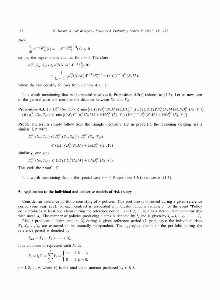
Now

ddt"s−1 7F

[s]Sn (t) =−"s−1 7F [s−1]Sn (t)6 0

so that the supremum is attained for t = 0. Therefore

dR+

s (SN ; SM )6 dNs (N;M)"

s−1 7F[s]Sn (0)

=1

(s− 1)!dNs (N;M)"

s−1ESs−1n = (EX1)s−1dNs (N;M);

where the last equality follows from Lemma 4.1.

It is worth mentioning that in the special case s = 0, Proposition 4.2(i) reduces to (1.2). Let us now turnto the general case and consider the distance between SN and TM .

Proposition 4.3. (i) DR+

s (SN ; TM )6 min{(EX1)sDNs (N;M)+EMDR+

s (X1; Y1); (EY1)sDNs (N;M)+ENDR+

s (X1; Y1)}.(ii) dR

+

s (SN ; TM )6 min{(EX1)s−1dNs (N;M) + EMdR+

s (X1; Y1); (EY1)s−1dNs (N;M) + ENdR+

s (X1; Y1)}:

Proof. The results simply follow from the triangle inequality. Let us prove (i); the reasoning yielding (ii) issimilar. Let write

DR+

s (SN ; TM )6DR+s (SN ; SM ) + D

R+s (SM ; TM )

6 (EX1)sDNs (N;M) + EMDR+

s (X1; Y1)

similarly, one gets

DR+

s (SN ; TM )6 (EY1)sDNs (N;M) + ENDR+

s (X1; Y1):

This ends the proof.

It is worth mentioning that in the special case s= 0, Proposition 4.3(i) reduces to (1.3).

5. Application to the individual and collective models of risk theory

Consider an insurance portfolio consisting of n policies. This portfolio is observed during a given referenceperiod (one year, say). To each contract is associated an indicator random variable Ii for the event “Policyno. i produces at least one claim during the reference period”, i=1; 2; : : : ; n; Ii is a Bernoulli random variablewith mean qi. The number of policies producing claims is denoted by I. and is given by I.= I1 + I2 + · · ·+ In.Risk i produces a claim amount Xi during a given reference period (1 year, say); the individual risks

X1; X2; : : : ; Xn are assumed to be mutually independent. The aggregate claims of the portfolio during thereference period is denoted by

Sind = X1 + X2 + · · ·+ Xn:It is common to represent each Xi as

Xi = IiVi =Ii∑j=1

Vi =

{Vi if Ii = 1;

0 if Ii = 0;

i = 1; 2; : : : ; n, where Vi is the total claim amount produced by risk i.


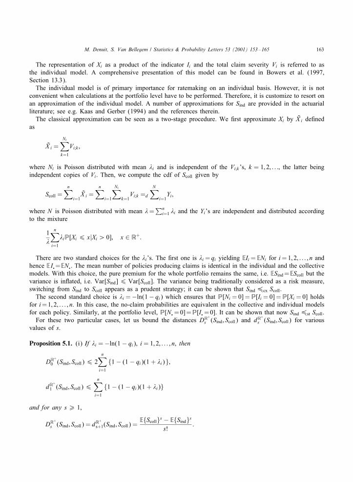
The representation of Xi as a product of the indicator Ii and the total claim severity Vi is referred to asthe individual model. A comprehensive presentation of this model can be found in Bowers et al. (1997,Section 13:3).The individual model is of primary importance for ratemaking on an individual basis. However, it is not

convenient when calculations at the portfolio level have to be performed. Therefore, it is customize to resort onan approximation of the individual model. A number of approximations for Sind are provided in the actuarialliterature; see e.g. Kaas and Gerber (1994) and the references therein.The classical approximation can be seen as a two-stage procedure. We 0rst approximate Xi by X̃ i de0ned

as

X̃ i =Ni∑k=1

Vi;k ;

where Ni is Poisson distributed with mean &i and is independent of the Vi;k ’s, k = 1; 2; : : :, the latter beingindependent copies of Vi. Then, we compute the cdf of Scoll given by

Scoll =n∑i=1X̃ i =

n∑i=1

Ni∑k=1Vi;k =d

N∑i=1Yi;

where N is Poisson distributed with mean &=∑ni=1 &i and the Yi’s are independent and distributed according

to the mixture

1&

n∑i=1

&iP[Xi 6 x|Xi ¿ 0]; x ∈ R+:

There are two standard choices for the &i’s. The 0rst one is &i = qi yielding EIi = ENi for i=1; 2; : : : ; n andhence E I.=EN.. The mean number of policies producing claims is identical in the individual and the collectivemodels. With this choice, the pure premium for the whole portfolio remains the same, i.e. ESind=EScoll but thevariance is inQated, i.e. Var[Sind]6 Var[Scoll]. The variance being traditionally considered as a risk measure,switching from Sind to Scoll appears as a prudent strategy; it can be shown that Sind 4cx Scoll.The second standard choice is &i =−ln(1− qi) which ensures that P[Ni = 0] =P[Ii = 0] =P[Xi = 0] holds

for i=1; 2; : : : ; n. In this case, the no-claim probabilities are equivalent in the collective and individual modelsfor each policy. Similarly, at the portfolio level, P[N.=0]=P[I.=0]. It can be shown that now Sind 4st Scoll.For these two particular cases, let us bound the distances DR

+

s (Sind ; Scoll) and dR+s (Sind ; Scoll) for various

values of s.

Proposition 5.1. (i) If &i =−ln(1− qi), i = 1; 2; : : : ; n, then

DR+

0 (Sind ; Scoll)6 2n∑i=1

{1− (1− qi)(1 + &i)};

dR+

1 (Sind ; Scoll)6n∑i=1

{1− (1− qi)(1 + &i)}

and for any s¿ 1,

DR+

s (Sind ; Scoll) = dR+s+1(Sind ; Scoll) =

E{Scoll}s − E{Sind}ss!

:


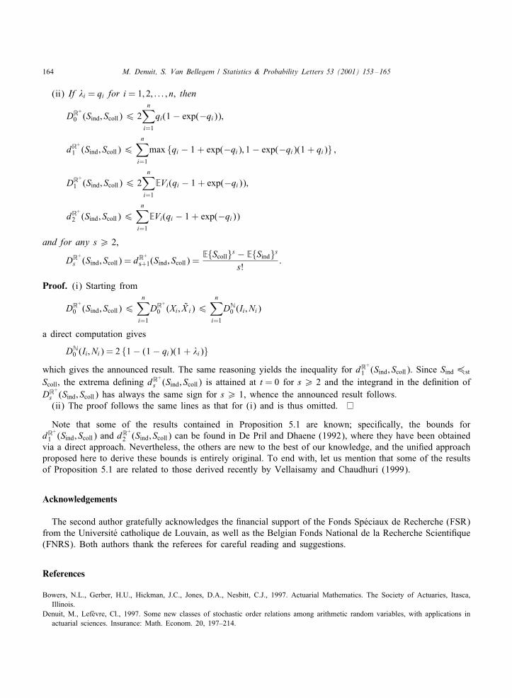
(ii) If &i = qi for i = 1; 2; : : : ; n, then

DR+


qi(1− exp(−qi));

dR+


max {qi − 1 + exp(−qi); 1− exp(−qi)(1 + qi)} ;

DR+


EVi(qi − 1 + exp(−qi));

dR+


EVi(qi − 1 + exp(−qi))

and for any s¿ 2,

DR+

s (Sind ; Scoll) = dR+s+1(Sind ; Scoll) =

E{Scoll}s − E{Sind}ss!

:

Proof. (i) Starting from

DR+


DR+

0 (Xi; X̃ i)6n∑i=1

DN0 (Ii; Ni)

a direct computation gives

DN0 (Ii; Ni) = 2 {1− (1− qi)(1 + &i)}which gives the announced result. The same reasoning yields the inequality for dR

+

1 (Sind ; Scoll). Since Sind 4st

Scoll, the extrema de0ning dR+

s (Sind ; Scoll) is attained at t = 0 for s¿ 2 and the integrand in the de0nition ofDR

+

s (Sind ; Scoll) has always the same sign for s¿ 1, whence the announced result follows.(ii) The proof follows the same lines as that for (i) and is thus omitted.

Note that some of the results contained in Proposition 5.1 are known; speci0cally, the bounds fordR

+

1 (Sind ; Scoll) and dR+2 (Sind ; Scoll) can be found in De Pril and Dhaene (1992), where they have been obtained

via a direct approach. Nevertheless, the others are new to the best of our knowledge, and the uni0ed approachproposed here to derive these bounds is entirely original. To end with, let us mention that some of the resultsof Proposition 5.1 are related to those derived recently by Vellaisamy and Chaudhuri (1999).

Acknowledgements

The second author gratefully acknowledges the 0nancial support of the Fonds Sp&eciaux de Recherche (FSR)from the Universit&e catholique de Louvain, as well as the Belgian Fonds National de la Recherche Scienti0que(FNRS). Both authors thank the referees for careful reading and suggestions.

References

Bowers, N.L., Gerber, H.U., Hickman, J.C., Jones, D.A., Nesbitt, C.J., 1997. Actuarial Mathematics. The Society of Actuaries, Itasca,Illinois.

Denuit, M., LefLevre, Cl., 1997. Some new classes of stochastic order relations among arithmetic random variables, with applications inactuarial sciences. Insurance: Math. Econom. 20, 197–214.


Denuit, M., LefLevre, Cl., Shaked, M., 1998. The s-convex orders among real random variables, with applications. Math. InequalitiesAppl. 1, 585–613.

Denuit, M., LefLevre, Cl., Utev, S., 1999. Stochastic orderings of convex=concave-type on an arbitrary grid. Math. Oper. Res. 24, 835–846.Denuit, M., LefLevre, Cl., Utev, S., 2000. Measuring the impact of dependence on the number of claimants in the individual model.Mimeo.

De Pril, N., Dhaene, J., 1992. Error bounds for compound Poisson approximation of the individual risk model. ASTIN Bull. 22, 135–148.Fishburn, P.C., Lavalle, I.H., 1995. Stochastic dominance on unidimensional grid. Math. Oper. Res. 20, 513–525. Erratum in Vol. 21,p. 252.

Finkelstein, M., Tucker, H.G., Veeh, J.A., 1990. The limit distribution of the number of rare mutants. J. Appl. Probab. 27, 239–250.Kaas, R., Gerber, H.U., 1994. Some alternatives for the individual model. Insurance: Math. Econom. 15, 127–132.Gerber, H.U., 1981. An Introduction to Mathematical Risk Theory. Huebner Foundation Monograph.Gerber, H.U., 1984. Error bounds for the compound Poisson approximation. Insurance: Math. Econom. 3, 191–194.LefLevre, Cl., Utev, S., 1996. Comparing sums of exchangeable Bernoulli random variables. J. Appl. Probab. 33, 285–310.LefLevre, Cl., Utev, S., 1998. On order-preserving properties of probability metrics. J. Theoret. Probab. 11, 907–920.M1uller, A., 1997. Stochastic orderings generated by integrals: a uni0ed study. Adv. Appl. Probab. 29, 414–428.Rachev, S.T., 1991. Probability Metrics and the Stability of Stochastic Models. Wiley, New York.Rachev, S.T., R1uschendorf, L., 1990. Approximation of sums by compound Poisson distributions with respect to stop-loss distances. Adv.Appl. Probab. 22, 350–374.

Shaked, M., Shanthikumar, J.G., 1994. Stochastic Orders and their Applications. Academic Press, New York.Vellaisamy, P., Chaudhuri, B., 1996. Poisson and compound Poisson approximation for random sums of random variables. J. Appl.Probab. 33, 127–137.

Vellaisamy, P., Chaudhuri, B., 1999. On compound Poisson approximation for sums of random variables. Statist. Probab. Lett. 41,179–189.

on the stop-loss and total variation distances between random sums

Documents