1

On the Suspension of Graded Sediment by Waves above Ripples : inferences

of convective and diffusive processes

A.G Daviesa, and P.D Thorneb

a Centre for Applied Marine Sciences, School of Ocean Sciences, Bangor University, Menai Bridge, Anglesey LL59 5AB U.K.

Corresponding author: Email: a.g.davies@bangor.ac.uk; Tel +44 (0)1248 383933

b National Oceanography Centre, Proudman Building, 6 Brownlow Street, Liverpool L3 5DA U.K. Email: pdt@noc.ac.uk

Abstract

The relationship between the grain size distribution of the sediment on the bed and that found in

suspension due to wave action above ripples is assessed here using detailed, pumped sample,

measurements obtained at full-scale and also at laboratory scale. The waves were regular and

weakly asymmetrical in most tests, and irregular in a minority of tests. The beds comprised fine and

medium sand and were rippled in all tests. The cycle-mean sediment concentrations (C) from the

pumped samples were split into multiple grain size fractions and then represented by exponential C-

profile shapes. The analysis of these profiles was carried out in two stages to determine: i) the

relationship between the size distribution of the sediment on the bed and that found in the

reference concentration, and ii) the behaviour of the exponential decay scale of the C-profiles. From

this analysis inferences are made about the relative roles of diffusion and convection in the upward

sediment flux linked to the process of vortex shedding from the ripple crests. The Transfer Function

(Tr) defined to relate the bed sediment size distribution to that of the reference concentration

indicates that, while finer fractions are relatively easily entrained, the suspension of some coarser

fractions is caused by an additional convective effect that supplements diffusion. The evidence for

this becomes pronounced above steep ripples, and the Transfer function suggests further that

irregular waves increase the occurrence of coarser fractions in suspension. A functional form for Tr

is suggested incorporating these principles. The exponential decay scale LS arising from the

fractional C-profiles is also examined to assess the mechanisms responsible for the upward transfer

of grains and a parameterisation of LS related to ripple size is suggested. The separate findings for Tr

and LS present supporting evidence of diffusion affecting the finer fractions in suspension and

combined diffusion + convection affecting the coarser fractions. The methodology developed allows

the vertical profile of suspended median grain size to be predicted given knowledge of both the bed

grain size distribution and also the flow conditions.

2

Keywords: Sediment transport; Waves; Graded sediment; Sand ripples; Reference concentration;

Suspended concentration profiles.

List of symbols

a coefficient in Eq. (A.2)

a1,a2 coefficients in ripple ‘flow contraction’ expression

A1 semi-orbital near-bed excursion amplitude based on the wave fundamental frequency

A (=D3) Archimedes Buoyancy Index

b coefficient in Eq. (A.2)

b1,b2 coefficients in Transfer function expression (Eq. (14))

B1,B2 dimensional coefficients with numerical values depending upon , s and g

c1-c4 empirical constants

C wave cycle-mean sediment concentration

C0,Ca,Cr sediment volumetric reference concentration at height z = 0, z=a and z=zr , respectively.

Cbi bed sediment volumetric concentration of the ith grain fraction

Cri volumetric reference concentration of the ith grain fraction ( < … > denotes a wave cycle-mean)

Ccb cumulative %-distribution of bed sediment sizes

Ccr cumulative %-distribution of reference concentration particle sizes

Ci(zj) suspended concentration of the ith grain fraction at the jth height z above the bed

Ccum,i(zj) cumulative concentration based on Ci(zj)

Csum(zj) total concentration summed over the i grain fractions at the jth height z above the bed

d sediment grain size; this includes sizes obtained by interpolating the discrete dm scale

dc maximum allowable or critical grain size in suspension

ds sieve size used in grain distribution analysis

dm grain size corresponding to central diameter for each sieve interval determined at the respective mid-

points on the scale

d50 median grain diameter of the sediment

d50b median grain diameter of the bed material

d50s median grain diameter of the sediment in suspension

di sediment grain diameter (bed or suspended material) for which i% of the grains are finer by volume

(or weight)

d0 (=2A1) near-bed orbital diameter

D dimensionless grain size (defined by Eq. (10))

fw wave friction factor (fw,max is maximum value according to Swart’s (1976) formula)

g acceleration due to gravity

H, Hs wave height, significant wave height

3

ks equivalent bed roughness

LS (=s/ws) decay (or distribution) length scale of the exponential C-profile

LST total decay (or distribution) length scale for the aggregated C-profile

Res Reynolds number of a settling grain (=wsd/),

RE wave Reynolds number (=U1A1/)

s (=s/) relative sediment density

T,Tp wave period, peak wave period

Tr ‘Transfer function’ relating the reference concentration to the bed sediment

u friction (or shear) velocity (with prime u’ : skin friction component)

uw peak value of friction (or shear) velocity during the wave cycle (with prime uw’ : as above)

U1,U2 first and second harmonics of the near-bed wave velocity amplitude

w upward fluid velocity (convective velocity in Fredsøe and Deigaard’s (1992) model)

ws sediment settling velocity

wsc settling velocity corresponding to the critical grain size in suspension dc

X non-dimensionalisation of grain diameter, defined by Eq. (14)

z height above the bed

za reference height above the bed at which C = Ca

zr height of reference concentration Cr

β (=s/m) quotient describing the local difference between the diffusion of a fluid ‘particle’ and a

discrete sediment particle

s near-bed layer thickness in which sediment diffusivity s remains constant

e estimated sediment diffusivity in Fredsøe and Deigaard’s (1992) convective model

m eddy viscosity, or vertical diffusion coefficient for momentum, in a clear fluid

s sediment vertical diffusivity

(=log2(d) with d in mm) Krumbein phi scale

ripple height

ripple wavelength

kinematic viscosity of water

Shields parameter, peak value during wave cycle (Eq.(12) (with prime : skin friction component)

density of water

s density of sediment

g (=(d84/d16)0.5) geometric standard deviation of the sediment

b bed shear stress ( < … > denotes a wave cycle-mean)

crit,i critical shear stress for the ith grain fraction of the bed sediment in isolation

e time scale of exchange in Fredsøe and Deigaard’s (1992) convective model

(=2/T) wave angular frequency

4

1. Introduction

Although the seabed sediment typically comprises a broad size distribution surprisingly little account

is taken of this in many of the methods used in sediment transport estimation. A single

representative grain size is generally used to characterise the sediment even though the seabed

includes both fine grain fractions that can readily be entrained into suspension, for example by

waves, and also coarse fractions that only ever form part of the bed load. The resulting grain size

distribution in suspension can be significantly different from that of the seabed. Further, due to the

larger settling velocities of the coarser fractions, the suspended sediment size distribution becomes

progressively dominated by finer grains as height above the bed increases. This has significant

implications, for example in relation to sediment sorting across beach profiles and to water quality

where contaminants are attached to finer or coarser particles. If the vertical sorting of sediment

grains between the bed surface material and the suspension, and hence the relative movement of

finer and coarser particles, is not taken into account, this may lead to bias and inaccuracy in

predicting net sediment transport rates. In a series of laboratory experiments involving different

sand mixtures beneath asymmetric waves, O’Donoghue and Wright (1994) showed that the relative

contributions to the net transport, in suspension and in the near-bed sheet flow layer, varied

significantly depending upon the sand size and grading.

Detailed procedures for modelling grain mixtures have remained rather ad hoc, with observations

suggesting that some grain size fractions in suspension can be far coarser than accounted for by

standard methodologies. For example, Masselink et al. (2007) estimated the sediment size in

suspension above oscillatory ripples at a coarse-grained beach site to be 0.6mm with settling

velocity 80 mm/s; these values are far larger than would be predicted by the turbulent diffusion

methodologies referred to later. This raises the interesting and important question: ‘Are all grain

fractions in suspension in a given flow influenced in the near-seabed layer by the same mixing

mechanisms?’ The answer is implicit in some previous works (e.g. Van Rijn, 1993), but we return to

the question here with the benefit of an extensive, detailed data set highlighting the suspension of

graded sediments by waves above rippled beds. While arguing that the answer is ‘No’, we infer from

the experimental data that, while the finer fractions in suspension are influenced primarily by

diffusion, the coarser fractions are progressively influenced also by convection. The present study is

in two parts, each involving suspended sediment data obtained beneath waves in both a full-scale

wave facility and also a laboratory flume. Initially we consider the relationship between the size

distribution of the sediment on the bed and that in suspension, and then the nature and causes of

5

the concentration profiles of the individual fractions in suspension. A similar study was carried out

for steady flow by Sengupta (1979) who related the size distribution of the bed material to that

obtained in suspension by pumped sampling at a fixed height above the bed. While Sengupta

produced results analogous to some of those presented in this paper, the nature of his observations

precluded discussion of the causes of the suspensions studied, which is a central aim here.

2. Background

2.1 Selective entrainment of graded sediment

Non-uniformity of the bed material results in selective entrainment processes commonly

represented by a hiding and exposure correction to the critical shear stress for the threshold of

motion (e.g., Egiazaroff, 1965). This increases the critical stress for finer particles and decreases it

for more exposed coarser particles (Wiberg and Smith, 1987; Van Rijn, 1993; Wallbridge et al., 1999;

Hassan 2003). In a multi-fraction approach Van Rijn (2007b) included an additional correction to the

shear stress itself due to Day (1980). The suspended concentration (C) can then be determined using

reference concentrations for the individual size fractions in the bed (Wallbridge and Voulgaris,

1997). Sistermans (2002) found, however, that for wave + current flows above rippled beds it was

not possible to predict near-bed reference concentrations per fraction satisfactorily using hiding and

exposure concepts, due to the sensitivity of such calculations and also lack of understanding of the

processes. Nielsen (1992), while noting that there was little information available about the

selective entrainment of different sand sizes under waves, proposed a simple ‘rule of thumb’ to

relate the sediment in the bed to that found in near-bed suspension (see §5 and Appendix B). The

uncertainties arising from Nielsen’s (1992) approach, together with the findings of Sistermans (2002)

and Hassan (2003) pointing to the difficulties in understanding selective entrainment processes,

have motivated here a different approach based on a ‘Transfer Function’ that links the sediment on

the bed to that in the flow.

The relationship between the suspended median grain size d50s and that of the bed material d50b

depends upon the degree of non-uniformity of the bed sediment expressed, for example, by the

quotient d90/d10. Based on experiments with irregular waves Van Rijn (2007b) noted that for

relatively ‘uniform’ bed sediment having d90/d10 = 1.8-2.1 the quotient d50s/d50b was in the range 0.7-

0.9, while for less uniform ‘graded’ material having d90/d10 4.7 the range was 0.35-0.45. Similar

conclusions were reached by Sistermans (2002). In both the rippled regime (Sistermans, 2002), and

6

also the oscillatory sheet-flow regime (Hassan, 2003), the suspended median size d50s has been

found to become smaller with increasing height above the bed.

2.2 Mixing in the wave boundary layer

Although the C-profiles investigated in this paper are wave cycle-averaged, their origin lies in the

intra-wave mixing processes in the wave boundary layer. These processes are fundamentally

different above plane and rippled beds formed, respectively, in oscillatory flows by waves having

large and small height. Above plane beds momentum transfer occurs primarily by turbulent

diffusion, whereas above steeply rippled beds momentum transfer and the associated sediment

dynamics are dominated by coherent, periodic vortex structures (Davies and Thorne, 2008). These

vortices are shed from the ripple crests at each flow reversal and dominate the near-bed dynamics in

a convective layer of thickness 1-2 ripple heights. Above this the coherent motions break down to be

replaced by random turbulence, with the overall effect that sand is entrained to considerably greater

heights above rippled beds than above plane beds.

Even above steeply rippled beds, the conceptual basis for the interpretation of (vertical) C-profiles is

normally taken as being turbulent diffusion. If temporal and also (horizontal) spatial variations in

such profiles are neglected, the balance between upward diffusion and downward settling is

expressed through the 1D-vertical (1DV) advection-diffusion equation:

𝑠𝑑𝐶

𝑑𝑧+ 𝑤𝑠𝐶 = 0 (1)

where C is the wave-averaged concentration at height z above the bed, s is the sediment diffusivity

and ws is the settling velocity. The sediment diffusivity is then usually related to the diffusion

coefficient for momentum, or eddy viscosity, for a clear fluid (m), as follows:

𝑠 = 𝑚 (2)

where for relatively low sediment concentrations the ‘damping’ of turbulence by suspended

sediment can be ignored (Li and Davies, 2001), and where the -factor then describes the difference

between the diffusion of a fluid ‘particle’ and a discrete sediment particle. It is not obvious that the

gradient diffusion assumption used in Eq. (1) should have any relevance in the oscillatory boundary

layer above ripples since the ‘free paths’ of the larger eddies responsible for momentum transfer are

not, in general, ‘small’ compared with the size of the mixing domain. This difficulty has been

addressed by Nielsen and Teakle (2004), while the basis of a diffusive modelling approach has been

considered by Davies and Villaret (1997) and Malarkey and Davies (2004). In practice, the

relationship between m and s may be more complicated than Eq. (2) suggests, with some finer

7

fractions in suspension being represented by this equation quite well, but other coarser fractions far

less well.

As far as the vertical structure of m above rippled beds in oscillatory flow is concerned, Davies and

Villaret (1997) found, for very rough turbulent flows having A1/ks<5, that in a layer of approximate

thickness 2, where is the ripple height, m is well represented by Nielsen’s (1992) height-

invariant, wave-averaged, expression for very rough beds, given by:

𝑚 = 𝑐1𝐴1𝑘𝑠 (3)

where A1 is the semi-orbital excursion amplitude near the bed, (= 2/T) is the wave angular

frequency (T = wave period), and the empirical constant c1 =0.004, with ks the equivalent bed

roughness, given by:

𝑘𝑠 = 25(𝜂

𝜆⁄ ) (4)

where is the ripple wavelength. A similar height-invariant formula for m was proposed by Sleath

(1991). The dynamical significance of eddy shedding is expected to become pronounced when /

0.1. In this case the solution of Eq. (1) for the suspended concentration becomes simply:

𝐶 = 𝐶0𝑒−𝑧 𝐿𝑠⁄ (5)

where LS (=s/ws) is the decay (or distribution) length scale, C0 is the wave-averaged ‘reference’

concentration at height z=0, with the -factor in Eq.(2) treated as a constant for a particular grain

size in suspension. For rippled beds in oscillatory flow, the cause of the ‘-effect’ has been analysed

by Malarkey et al. (2015); Nielsen (1992) suggested that is equal to about 4, a value found

appropriate by Thorne et al. (2002) and Davies and Thorne (2005).

The -effect has been found to occur also above ‘dynamically plane’ beds comprising ripples of low

steepness which induce less vortex shedding. Above such beds the mixing length scale is normally

assumed to increase with height and the eddy viscosity is taken in the form

𝑚 = 𝑐2𝑢∗𝑧 (6)

where u is an appropriate shear velocity and c2 is a constant. In this case the solution of Eq. (1),

subject again to Eq. (2), becomes

𝐶 = 𝐶𝑎(𝑧𝑎

𝑧⁄ )𝑤𝑠

𝑐2𝛽𝑢⁄

(7)

where Ca is the reference concentration at height z=za. Sistermans (2002) tested 10 different

functional forms for the vertical profile of the sediment diffusivity s, including Eqs. (3) and (6), and

concluded that, for irregular waves + current above a rippled bed, turbulent diffusion can describe

the C-profiles and also the d50s profile if size grading is taken into account (see Appendix A). In the

8

experiments referred to in §2.1, Sistermans (2002) noted that higher suspended concentrations

occurred for ‘graded’ sediment than for more ‘uniform’ sediment, but with the respective near-bed

reference concentrations being approximately equal. The implied s value was somewhat larger (by

~10%) for the graded sediment in these tests.

Above dynamically plane beds in steady flow, Van Rijn (1984) analysed C-profiles measured by

Coleman (1981) and obtained the expression:

𝛽 = 1 + 2(𝑤𝑠

𝑢∗⁄ )

2 𝑓𝑜𝑟 0.1 <

𝑤𝑠𝑢∗

⁄ < 1 (8)

According to Eq. (8), the increase in the effective sediment diffusivity is greater for relatively larger

(i.e. faster settling) particles in suspension. Van Rijn suggested that this this was due to the

increasing influence of centrifugal forces even in steady cases where eddy shedding from the bed is

less well organised than in oscillatory flows. However Sistermans (2002) reanalysed Coleman’s data

and could not find any dependence of β on the suspended sediment size. Nevertheless Van Rijn

(2007a) incorporated Eq.(8) in his more recent formulation for wave and current flows.

In practice, very few formulations for s have taken account of the -effect. A notable exception was

that of Van Rijn (1989) (see Van Rijn, 1993) for unsteady flow based on s being height-invariant in a

near-bed layer of thickness s. Above rippled beds, s was taken equal to 3 implying shed-eddy

sizes that scale on the ripple height. Van Rijn’s (1989) formula for s utilises Eqs. (2) and (3), with ks

taken equal to s and, importantly, with effectively taken equal to the dimensionless grain size D

as follows:

휀𝑠 = 𝑐1𝐷∗𝐴1𝜔𝛿𝑠 (9)

where

𝐷∗ = 𝑑 ((𝑠 − 1)𝑔

𝜈2⁄ )1 3⁄

(10)

with s=s/ (s = sediment density, = water density), g = acceleration due to gravity, and =

kinematic viscosity of water. So again the greater is the grain size d in suspension the greater is s

according to Eq. (9), the D parameter expressing the increased mixing observed for larger particles.

Van Rijn’s (2007a) more recent expression for s has the same general height-constant nature as Eq.

(9) in the near-bed layer, but with c1D replaced by 0.018β (wherein the peak value uw during the

wave cycle is used in Eq. (8)) and with s replaced by 2w where w is the thickness of the wave

boundary layer (see Van Rijn (2007a) for the details). This formulation also caps the value of at 1.5

which limits the mixing of the larger suspended particles. Both of Van Rijn’s formulations for s are

compared with the present data in §6.

9

2.3 Convection and diffusion in the wave boundary layer

The sediment mixing giving rise to the C-profile is linked to the other main issue addressed here,

namely the relationship between the sediment size distribution on the bed and that in suspension.

A commonly used criterion to determine whether or not a sediment grain will be entrained is that of

Fredsøe and Deigaard (1992). They suggested that a particle should be able to remain in suspension

provided that its settling velocity (ws) is sufficiently small compared with the near-bed vertical

turbulent velocity fluctuations, the magnitude of which are of the order of the (skin friction) shear

velocity 𝑢 . Davies and Thorne (2002) used this criterion to define the maximum allowable, or

critical, grain size in suspension (diameter = dc) to be that having settling velocity 𝑤𝑠𝑐 = 0.8 𝑢𝑤

where 𝑢𝑤 is the peak wave-induced skin-friction shear velocity. However, for the wave conditions

studied, including some of the same experiments considered later, they found that this essentially

diffusive approach failed to account fully for the rapid increase observed in d50s on approaching the

bed, caused by the presence of coarse fractions having size significantly larger than dc.

The presence in suspension of grains having d>dc points to a mechanism other than turbulent

diffusion to balance sediment settling. Fredsøe and Deigaard (1992) considered the effect of an

upward convective flux of sediment arising from either vortex shedding above ripples in oscillatory

flow or from coherent motions arising from the bursting process in steady flow. In their convection

model, upward moving (with constant velocity w) parcels of sediment-laden fluid exchange water

and sediment (with time scale of exchange e) with the surroundings in which the concentration is

assumed to be very much smaller than in the parcel itself. The parcel travels upwards with constant

velocity exchanging fluid and sediment as it does so. The steady-state balance between settling in

the surrounding fluid (with velocity ws) and upward vertical convection gives rise to a mean

concentration profile that decays exponentially with height. When this profile is analysed in order to

determine the implied, estimated turbulent diffusion coefficient (e) in equation (1) it turns out that

e = wswe indicating an apparent diffusion coefficient that increases with the settling velocity.

Treating w and e as constants, Fredsøe and Deigaard’s convection argument leads to the conclusion

that e/w

s = constant and, thus, that the relative suspended concentration will be the same for all

grain sizes. Tomkins et al. (2003) observed this effect for regular waves above a rippled bed of

mixed quartz and heavy mineral sand. The vertical gradients of the time-averaged suspended C-

profiles were found to be similar for the light and heavy minerals, despite their settling velocities

differing by a factor of about 1.5, implying a convective rather than diffusive distribution mechanism,

at least for the heavy particles. Fredsøe and Deigaard’s model was not intended to be a quantitative

10

description, but simply an illustration of the process of convection. The same comment can be made

about the behavioural model of Nielsen (1992) in which the process of ‘pure convection’ leads again

to the relative suspended concentration being the same for all grain sizes. All this evidence seems to

point to the need for a quantitative approach including a convective element to represent the

coarser fractions in suspension.

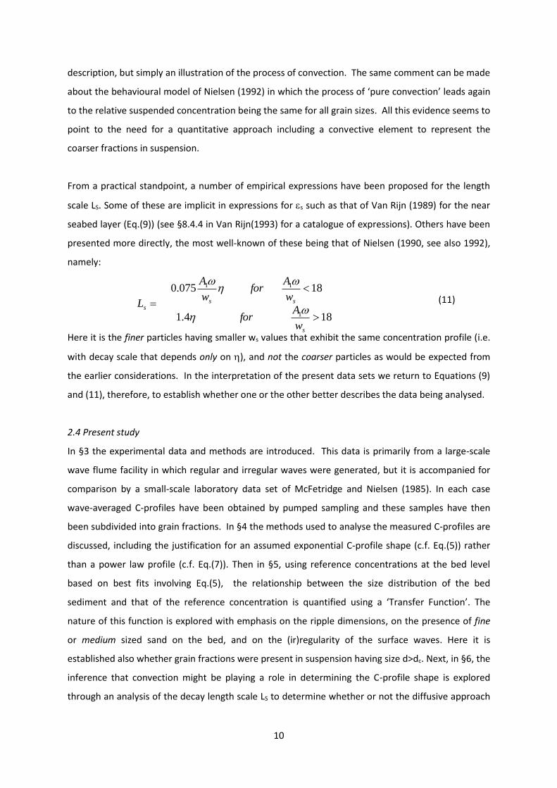
From a practical standpoint, a number of empirical expressions have been proposed for the length

scale LS. Some of these are implicit in expressions for s such as that of Van Rijn (1989) for the near

seabed layer (Eq.(9)) (see §8.4.4 in Van Rijn(1993) for a catalogue of expressions). Others have been

presented more directly, the most well-known of these being that of Nielsen (1990, see also 1992),

namely:

(11)

Here it is the finer particles having smaller ws values that exhibit the same concentration profile (i.e.

with decay scale that depends only on ), and not the coarser particles as would be expected from

the earlier considerations. In the interpretation of the present data sets we return to Equations (9)

and (11), therefore, to establish whether one or the other better describes the data being analysed.

2.4 Present study

In §3 the experimental data and methods are introduced. This data is primarily from a large-scale

wave flume facility in which regular and irregular waves were generated, but it is accompanied for

comparison by a small-scale laboratory data set of McFetridge and Nielsen (1985). In each case

wave-averaged C-profiles have been obtained by pumped sampling and these samples have then

been subdivided into grain fractions. In §4 the methods used to analyse the measured C-profiles are

discussed, including the justification for an assumed exponential C-profile shape (c.f. Eq.(5)) rather

than a power law profile (c.f. Eq.(7)). Then in §5, using reference concentrations at the bed level

based on best fits involving Eq.(5), the relationship between the size distribution of the bed

sediment and that of the reference concentration is quantified using a ‘Transfer Function’. The

nature of this function is explored with emphasis on the ripple dimensions, on the presence of fine

or medium sized sand on the bed, and on the (ir)regularity of the surface waves. Here it is

established also whether grain fractions were present in suspension having size d>dc. Next, in §6, the

inference that convection might be playing a role in determining the C-profile shape is explored

through an analysis of the decay length scale LS to determine whether or not the diffusive approach

184.1

18075.0

1

11

s

sss

w

Afor

w

Afor

w

A

L

11

breaks down for the coarser fractions. The methods developed in §5 and §6 are used in §7 to

recover profiles of d50s. Some of the wider implications of the results are then discussed in §8 and

the conclusions are presented in §9.

3. Experiments and Observational Methods

3.1 Experiments in a full-scale wave flume

Detailed measurements of sediment in suspension above ripples were made during a series of

campaigns in the Deltaflume of Delft Hydraulics, now Deltares (Williams et al., 1998). The large size

of this flume (230 m long, 5 m wide and 7 m deep) allowed the wave and sediment transport

phenomena to be studied at full scale. A wave generator at one end of the flume produced either

regular or irregular waves that propagated over the sediment test bed before dissipating on a beach

at the opposite end. Two series of experiments are considered from which specific tests have been

subject to detailed sediment analysis, namely a set of 4 tests carried out above a bed of fine sand

(median diameter d50=0.162 mm, geometric standard deviation g=(d84/d16)0.5=1.7), and a set of 6

tests above a bed of medium sand (d50=0.329 mm, g=1.55). The majority of the tests were carried

out with regular, weakly asymmetric waves having heights, H, and periods, T, in the ranges 0.4-1.3 m

and 4-6 s, respectively. In addition, irregular waves (JONSWAP spectrum) were generated in 1 test

above the fine sand and 2 tests above the medium sand, having significant heights (Hs) and peak

periods (Tp) in the ranges 0.7-1.1 m and 4.7-5.1 s. Table 1 provides a list of the wave conditions

measured by two surface-following wave probes. The sediment beds of thickness 0.5 m and length

30 m were placed approximately half way along the flume, above which the water depth was 4.5 m.

To establish equilibrium conditions for the hydrodynamics and sediment transport, the waves

propagated over the bed for about 1 hour before data were recorded.

The measurements were made primarily using the instrumented tripod platform ‘STABLE’ (Sediment

Transport And Boundary Layer Equipment). The main cluster of instruments on STABLE was directed

towards the wave generator. This comprised a triple-frequency acoustic backscatter system (ABS),

with associated pumped sampling, and electromagnetic current meters (ECMs) at three heights

above the bed (0.30, 0.61 and 0.91 m). The ripples were measured using an acoustic ripple profiler

(ARP). This system uses a radially rotating 2 MHz acoustic pencil beam to measure a 3 m profile

along the bed. Measurements of ripple profiles were made approximately every 60 s during the

tests. Full details of the experimental set up and instrumentation were given by Thorne et al.

(2002,2009), and the minimal impact that STABLE had on the flow and bed forms was discussed by

12

Williams et al. (2003). The present analysis is concerned with (i) pumped sample data collected at 10

heights above the bed between 0.05 and 1.55 m, (ii) output from the ARP which gave detailed

measurements of the bed morphology, (iii) hydrodynamic measurements from the wave gauges and

ECMs and (iv) output from the ABS system, which was used here only to reference the bed location.

The novel feature of the present paper is the pumped sample data which has not previously been

analysed in detail.

Ripples formed on the bed with heights, , and wavelengths, , in the respective ranges 0.01-0.07 m

and 0.2-0.9 m for the fine sand, and 0.04-0.07 m and 0.28-0.51 m for the medium sand (see Table 1).

The corresponding ripple steepness / was <0.1 in the former cases and >0.1 in the latter. The

method by which the ripple dimensions were determined from the ARP results is described in §4.2.

The duration of each test was 1024 s, during which the ripples tended to migrate in the direction of

wave propagation. This was reflected by slight asymmetry in the profile shapes particularly in the

tests with regular waves.

The bed elevation was tracked during each test using the backscatter returns at the three ABS

frequencies (1, 2 & 4 MHz). The nearest range of the bed from the ABS was considered to be the

ripple ‘crest’ range. It was not always clear from the ABS time series that a ripple crest had, in fact,

passed beneath a particular transducer since, in some tests, the bed forms migrated by less than a

full wavelength. However, for this study this ‘nearest’ range has been treated as the crest of a ripple

where z=0 (z = height above the crest level). The bed level itself was determined to an accuracy of

5 mm from a clearly defined echo in the ABS returns (Thorne et al., 2002).

Much of the analysis that follows rests on measurements of sediment concentration made by

pumped sampling; here the procedures of Bosman et al. (1987) guided the sampling methodology.

Samples of suspended sediment were obtained at 10 heights above the bed in the range 0.05 to 1.55

m using two arrays of intake nozzles (diameter 4mm) oriented at 90 to the wave orbital motion.

Each nozzle was connected to a plastic pipe through which a mixture of water and sediment was

drawn to the surface through a peristaltic pump. The resulting simultaneous water/sand mixture

from each sampling position was collected in 10 litre buckets. Once full, the sediment was allowed

to settle and the excess water was poured away. The pumped sampling duration was about 15 min,

which corresponded typically to 180 wave cycles. All samples were sealed in plastic bags for

subsequent grain size and settling velocity analyses, and also for measurement of the suspended,

wave-averaged, sediment concentration. Although pumped sample measurements were made in

13

the nominal height range 0.05 to 1.5 m above the bed, size analysis was generally restricted to

heights below ~0.5 m due to the reduced sediment mass collected above this. The grain size

analyses reported here were carried out by a contractor using standard sieving techniques which,

depending upon individual test conditions, resulted in the C-profiles being subdivided into up to 15

fractions with a ¼- increment (=log2ds where ds is the grain diameter corresponding to the sieve

size in mm). The grain size distribution of the bed material was also determined by sieving bottom

samples. Figure 1 shows the cumulative %-finer grain size distribution curves for the two sand sizes

used in the Deltaflume, and also for the fine sand used in the laboratory experiment of McFetridge

and Nielsen (1985) [hereafter MN85] described in §3.2.

3.2 Experiment in a small scale wave flume

For comparison with the 10 tests from the Deltaflume, a similar experiment carried out at small-

scale by MN85 in a wave flume at the University of Florida is also considered. This provides both an

independent assessment of the results from the Deltaflume and also some insight into whether any

significant differences might occur between experiments carried out at full- and small-scale. The

flume was 18.3 m long, 0.61 m wide and 0.91 m deep. Waves were generated by a piston-type wave

maker at one end of the flume while a beach slope was present at the other end. Two series of tests

were carried out, one with natural ripples, the other with artificial ripples (triangular strip

roughness), though only the natural ripples are considered here. The hydrodynamic conditions (see

Table 1) involved weakly asymmetrical waves of height 0.130 m and period 1.51 s in water of depth

0.30m. MN85 used stream function theory to estimate the peak forward and backward near-bed

velocities as 0.278 and 0.216 m/s, respectively. Here this has been re-interpreted as being

equivalent to a Stokes 2nd order wave having first and second harmonic velocity amplitudes of: U1 =

0.247 m/s, U2 = 0.031 m/s.

The sand bed was constructed in the central 3.15 m of the flume to a depth of 0.1 m. The bed

comprised natural beach sand, but with the finer fractions augmented by the addition of quartz sand

(~10% of the total). The resulting size distribution shown in Figure 1, while being similar to that of

the fine sand used in the Deltaflume, departed from the classical lognormal distribution. MN85

quoted a mean grain diameter of 0.256 mm but, based on their cumulative grain size distribution,

the analyses later in this paper have used: d50=0.172 mm, g=1.86. A multi-intake tube array was

used to obtain a vertical profile of simultaneous, wave-averaged concentrations. The sampler array

was constructed of 3 mm diameter copper tubing with intakes having a vertical spacing of ~10 mm.

Nine intakes oriented perpendicular to the flow were used to sample the ~0.09 m closest to the bed.

14

Each pumped sample was divided into 6 grain size fractions with C-profiles presented for each

fraction. MN85 analysed 240 pumped samples obtained during 5 repeated tests. The sand ripples

during these tests were uniform and regular, with steepness significantly larger than the ripples in

the fine sand in the Deltaflume (see Table 1).

4. Analysis of Waves, Ripples and Suspended Sediment Concentration Profiles

4.1 Near-bed velocity field and bed shear stress

It was found by Thorne et al. [2002] that, if linear wave theory is used to calculate the near-bed

velocity amplitudes corresponding to the measured wave heights (H) and periods (T) given in Table

1, the results overestimate the amplitude of the first-harmonic (i.e. fundamental) component U1

(=A1) measured by the ECMs on STABLE (at heights of 0.30, 0.61 and 0.91 m above the bed) by 9%

3%. Although this could have been due in part to the presence of STABLE itself, it is also the case

that, since the waves were slightly asymmetric (i.e. weakly steep crested), linear theory may not

provide a sufficiently accurate representation of the velocity field. In order to provide realistic

inputs for the present calculations, a 9% reduction has been applied to the wave heights in Table 1

[following Thorne et al., 2002] and Stokes second-order theory has then been used to provide the

near-bed values of U1 and the amplitude of the second harmonic U2 given in Table 2 (see Davies and

Thorne (2005) for further explanation). Although this earlier procedure was developed for regular

waves above the medium sand bed, including tests a8a, a11a, a20a & a21a, it has been extended

here to both the fine sand and also irregular wave tests. The resulting near-bed asymmetry

parameter ratio U2/U1 never exceeded 0.066, indicating the presence of weakly asymmetric waves.

In the laboratory test of MN85 this ratio was somewhat larger (U2/U1 = 0.125).

Also listed in Table 2 for all tests are the corresponding values of: i) the near-bed orbital diameter

(d0=2A1); ii) the critical (maximum) grain size (dc) expected in suspension calculated using Fredsøe

and Deigaard’s criterion with 𝑢𝑤 = (

1

2𝑓𝑤)

12⁄

𝑈1 wherein the wave friction factor fw has been

determined using Jonsson’s formula as expressed by Swart (1976) (Eq. (12)) and with wsc given by

Hallermeier’s (1981) formulation for the settling velocity (Appendix C); iii) the Shields parameter

(skin friction) given by

=𝑢𝑤

2

(𝑠 − 1)𝑔𝑑50𝑏⁄ , 𝑓𝑤 = 𝑒𝑥𝑝 [5.2 (

𝐴1

2.5𝑑50𝑏)

−0.19

− 6] , 𝑓𝑤,𝑚𝑎𝑥 = 0.3 ; (12)

iv) the wave Reynolds number RE (=U1A1/), v) the relative roughness A1/ks with ks given by Eq. (4),

and vi) the number of analysed grain fractions available for each test from the pumped sampling.

15

Wiberg and Smith (1987) noted that, for mixed sediment beds, there are two length scales of

importance: the diameter of the grain fraction of interest, and the local roughness scale of the

surrounding bed which contributes to Eq. (12) through ks=2.5d50b.

For the Deltaflume tests, RE and A1/ks lie predominantly in the ranges (0.83-2.5)105 and (1.9-4.5),

which correspond to the very rough / rippled regime (see the delineation of Davies and Villaret

(1997), also Davies and Thorne (2008)). The test of MN85 (RE=0.11105, A1/ks=1.5) was carried out in

the same turbulent flow regime.

4.2 Ripple dimensions

Figure 2 shows examples of ripple evolution measured using the ARP in the fine and medium sand

during tests f5a and a8a. The ripples in the fine sand test, while being of somewhat larger

wavelength than those in the medium sand (see Table 1) , were not only of smaller steepness, but

were also less regular in shape with small secondary features occurring on the crests and also in the

troughs of larger features. Some ripple migration occurred in the fine sand (Figure 2a), but this

effect was more pronounced in the medium sand (Figure 2b).

To obtain the ripple height and wavelength, each ARP profile from the Deltaflume was processed

and mean values obtained for the experiment as a whole (see Thorne et al. (2001) for details).

Initially, each ripple profile was de-trended and given a zero mean. The ripple wavelength was

then obtained from the zero crossing points which were averaged over the profile length. To

estimate the ripple height the absolute value of the zero-mean measured profile was taken, from

which peaks were identified yielding the mean ripple height. The values of and obtained for

each profile were averaged to give the mean values listed in Table 1. Due to the complicated nature

of the bed forms in some cases, this ‘automated’ method was checked by a direct visual

interrogation of the ARP output. In the small-scale test of MN85 the ripple dimensions were

determined by direct measurement through the glass side-wall of the flume.

The results in Tables 1 and 2 indicate that the quotient d0/ was in the range (1-1.7) for the fine sand

and (1.8-2.3) for the medium sand tests in the Deltaflume, while d0/ was equal to about 1.5 for the

test of MN85. For the steeper ripples (/>0.1) this suggests a more organised pattern of vortex

shedding for MN85 than for the medium sand cases (see §6). Further, since the fine sand cases in

the Deltaflume had /<0.1, this might have been expected to limit the effectiveness of vortex

shedding in the sediment entrainment process. Figure 3 shows the ripple dimensions in Table 1

16

scaled according to the prediction scheme of Wiberg and Harris (1994) which distinguishes between

orbital, sub-orbital and anorbital ripples. This predictor is introduced here only to set the data

within the familiar parameter ranges, rather than to imply its appropriateness. Following Davies and

Thorne (2005, see Figure 7) the scheme has been modified by the application of a cap on the

steepness / of 0.14, which was found to be appropriate for the medium sand tests in the

Deltaflume, some of which are repeated here, and which fell in the sub-orbital range. In addition

Figure 3 includes the test of MN85 which falls in the middle of the orbital range and which is

described well by the scheme. The fine sand cases from the Deltaflume exhibit longer wavelength

and smaller steepness than predicted for sub-orbital ripples. However this behaviour has become

well documented, as noted by Nelson et al. (2013). By continuing to increase in wavelength, but

decrease in height and steepness, as d0/d50b increases these ripples can be categorized as ‘long wave

ripples’ (see Soulsby, Whitehouse and Marten, 2012). Their effect on the measured C-profiles is

explored in §6.

4.3 C-profiles and reference concentration

A significant step in the methodology concerns the choice made between fitting the measured C-

profiles to an exponential profile (Eq.(5)) rather than a power law profile (Eq.(7)). In wave-induced

flow, the former profile shape is usually expected to exist above a rippled bed while the latter is

expected above a ‘dynamically plane’ bed. Here, as seen in Table 1, relatively steep ripples were

found in the medium sand, while ripples of lower steepness were found for the fine sand (apart from

the laboratory case of MN85). Furthermore each test involved multiple fractions of which some

might have been better described by Eq.(5) and others by Eq.(7), or vice versa. Since the respective

C-profile shapes are associated with height-invariant and linearly increasing sediment diffusivities, a

generally applicable approach could involve a ‘constant + linear’ diffusivity profile (see Appendix A).

However this has not been implemented here both due to the preponderance of exponential profile

shapes in the pumped sample data, and also to preserve a basis for comparison with the previous

literature.

For all of the tests carried out in the Deltaflume both exponential (log-linear) and power law (log-log)

best fits were obtained for each grain fraction. Figure 4 shows the C-profiles obtained for the 14

fractions analysed for test a8a, together with the best fit exponential C-profile with 95% confidence

limits included. The reference concentrations used in §5 were obtained from the intercepts at

height z = 0, while the slopes provided the distribution length scales LS used later in §6. For the tests

with medium sand, the comparison between log-linear and log-log plotting indicated that an

17

exponential fit was better for all of the smaller fractions analysed, while for some of the larger

fractions a power law fit was just as good. For test a11a, an exponential fit was better for all

fractions. In contrast, for the tests with fine sand the picture was less clear-cut; tests f5a and f8a

were far better described by an exponential fit for all fractions, while test f7a seemed better

described by a power law fit for all fractions. Test f3a was somewhere in-between, with an

exponential fit being clearly better for all of the smaller fractions and for most fractions overall.

Despite some uncertainty however, it has seemed well justified to proceed with the simplifying

assumption that all fractions, in all tests, follow an exponential C-profile shape. An explanation as to

why such a profile is particularly effective is suggested in Appendix A. MN85 took this approach also

and the results quoted later are based on their best exponential fit outcomes for each of the 6

fractions analysed.

Figure 5 shows the reference concentrations obtained for the Deltaflume tests, with standard

deviation error bars included. For each test two values are plotted against the Shields parameter

(skin friction) (see Table 2); the symbols , x and correspond to the sum of the concentrations

obtained for the individual fractions, while the symbols , O and correspond to the best fit

obtained to the total aggregated C-profile. This latter fit produces a lower value of reference

concentration for each test, apart from that of MN85 for which the two values are similar. [The

reason for this difference is that, if two different exponential C-profiles are added, and a third

exponential curve is fitted to the resulting convex, but not strictly exponential, shape, this best fit

will have an intercept that is smaller than the notional reference concentration; see Figure 6 of

Davies and Thorne (2002) for an illustration.] While the reference concentration in Figure 5

generally increases with increasing , it exhibits significant scatter, similar to that in the equivalent

figure of Nielsen (1986, Fig. 2). The present paper is predicated on the existence of a sediment

suspension, and does not treat the magnitude of the aggregated reference concentration any

further (see Davies and Thorne (2005) for some further discussion). Instead the focus in what

follows is the relative behaviour of the different grain fractions comprising the suspended load.

5. Reference concentration for grain fractions

The volumetric reference concentrations determined for the Deltaflume data are shown for four

representative cases in Figure 6, each of which displays the same generally coherent behaviour. The

grain size plotted on the horizontal axis denotes the central diameter dm for each sieve interval

determined at the respective mid-points on the scale (c.f. Figure 4), rather than the sieve -size ds

18

itself (c.f. Figure 1). Also shown are the reference concentrations determined at the crest level by

MN85. For comparison with previous methods used to estimate fractional reference concentrations,

each subplot includes predictions based on both Nielsen’s (1992) near bed concentration (Eq. (B.1),

see Appendix B) and also a formulation of the kind used by Wallbridge and Voulgaris (1997). This

fractional, cycle-mean, reference concentration Cri has been taken as proportional to

𝐶𝑏𝑖 (⟨𝜏𝑏⟩ − 𝜏𝑐𝑟𝑖𝑡,𝑖) 𝜏𝑐𝑟𝑖𝑡,𝑖⁄ where Cbi is the volumetric bed concentration of the ith fraction, <b> is a

representative mean bed shear stress which has been obtained from <’>=’/2 and crit,i is the

critical shear stress derived from Shields curve for the ith fraction in isolation with no

hiding/exposure effects included. The calculations of crit,i have been made using Soulsby’s (1997)

Eq. SC (77). Each of the dashed lines has been scaled such that its aggregated sum is equal to that of

the observed reference concentration, and so only the patterns in Figure 6, and not the absolute

values, have significance. The relationship between Cri and Cbi is consistent in each subplot and the

two fractional methods produce fairly similar results that agree best with the present observations

for the medium sand. For the fine sand, the qualitative comparisons are less convincing, with the

fractional approaches tending to follow the bed size distribution too closely. As shown in Appendix

B, the resulting overestimation of the coarser fractions leads to a different outcome compared with

the approach (Eq. (13)) proposed in what follows, which is based on the relationship between the

cumulative grain size distributions for the reference concentration and the bed sediment.

To this end the fractional, measured, reference concentrations, c.f. Figure 6, have been expressed as

a cumulative distribution for each test, as shown in Figures 7a and 7b in comparison with the

distribution for the corresponding bed material. As expected the distribution curve for the reference

concentration lies in every case to the left of that for the bed material, indicating the presence of

generally finer material in suspension than is present on the bed, with the differences in the

reference concentration curves reflecting the different test conditions.

In order to compare the reference concentration and bed sediment distributions, the ‘raw’ curves

plotted in Figure 7 have been interpolated onto common grain diameter axes with an increment of 1

m for the fine sand and 2 m for the medium sand. This (spline-) interpolation was necessary due

to the different bed and suspended grain size intervals in Figure 7. [This refined grain size scale,

based on interpolation of the discrete values dm, is referred to hereafter by symbol d.] Thus it has

been possible to define a continuous ‘Transfer function’ Tr relating the suspended sediment to the

bed sediment by forming the quotient:

𝑇𝑟 =100−𝐶𝑐𝑟

100−𝐶𝑐𝑏 (13)

19

where Ccr and Ccb are the cumulative %-distributions for the reference concentration and bed

sediment, respectively. The function Tr simply represents the broad trends in the relationship

between the distributions shown in Figure 7, without recourse to hiding and exposure

considerations for individual fractions. For grain sizes less than about 50 m, for which data is

sparse, the vagaries of the interpolation have been prevented from producing larger %-values for

the bed sediment than for the reference concentration. It follows that the value of Tr is capped at

unity for small grain sizes; as the grain size increases Tr then decreases indicating the successively

lower level of transfer of bed particles into suspension. Figure 8 shows that the Transfer function

has a consistent pattern in all tests and, as expected, there is a clear separation between the fine

sand (blue/cyan curves) and medium sand (red/green) curves. As indicated in Figure 6, Nielsen

(1992) suggested a simple ‘selective entrainment’ function to relate the sediment in the bed to that

found in near-bed suspension. However, when interpreted as a Transfer function Tr, Nielsen’s

(1992) Eq. (B.1) turns out to overestimate the importance of the coarser fractions in the reference

concentration (see Appendix B). It may be expected from the comparisons in Figure 6 that the same

bias is inherent in fractional approaches such as that used by Wallbridge and Voulgaris (1997),

motivating the use of the alternative Transfer function approach.

Figure 9 shows the same results for Tr but with the grain size normalised by the critical diameter dc.

All tests show evidence of sediment in suspension for d/dc >1 suggesting that a convective

mechanism, as well as turbulent diffusion, is responsible for the upward flux of sediment. The

presence in suspension of grains having d>dc is far more pronounced for the medium sand

Deltaflume cases than the fine sand cases, with the steeper ripples formed in the medium sand

being more capable than the low ripples in the fine sand of suspending coarser fractions. This

reinforces the suggestion of a convective transfer mechanism associated with vortex shedding from

the steeper ripple crests. Interestingly, the fine-sand case of MN85, in which the ripples were also

steep (/=0.14), exhibits a Transfer function similar to that found for some of the steeply-rippled,

medium-sand cases in the Deltaflume. The scaling of grain size by dc in isolation in Figure 9 is

evidently not sufficient to explain the functional form of Tr, since the fine and medium sand

groupings remain fairly distinct. So the question that arises is whether a non-dimensional scaling of

the grain diameter can be found that ‘collapses’ the curves in Figure 8 in a way that brings out the

underlying behaviour of the Transfer function.

The scaling approach adopted in Figure 10 involves the introduction of the peak bed shear stress,

together with a ripple steepness factor. The former dependence is empirically based and has been

20

arrived at simply by noting how the ordering of the Tr curves in Figure 9 for the different tests is

correlated with the values of ’ in Table 2. As far as the rippled bed effect is concerned, ‘flow

contraction’ terms of the kind used by Nielsen (1986) have been tested, involving the general

expression (1+a1(/))a2 where a1,2 are constants that depend upon the ripple geometry. For

sinusoidal ripples the enhancement of the irrotational flow speed at the ripple crest compared with

that in the free stream corresponds to a1=1 and the choice a2=2, which implies a quadratic friction

effect, then provides an enhancement to the bed stress based on the enhancement in the near-bed

flow speed. For steep natural ripple shapes Davies (1979) modelled the potential flow and showed

that values of a1=2 (or larger) were appropriate depending upon the detailed ripple shape. For the

present tests the value a1=3, combined with a2=2, has been found to give the most convincing

representation of the Transfer function Tr. In practice, this empirical ‘flow contraction’ expression

(with a1=3 and a2=2) behaves in a closely similar manner (trend within 3%) to the ripple steepness

itself for all the ripples in the present tests having />0.05, that is apart from f7a for which / was

somewhat smaller. Therefore, the rippled bed effect has been taken here simply as /, with a

correction made for f7a.

With both the bed stress and also rippled bed effects included, the abscissa has been scaled using

the parameter X defined in Eq. (14). This draws the Tr curves together quite well and, interestingly,

causes the three irregular wave tests (f7a, a9a and a10a) to stand apart from the others. This

separation is highlighted in Figure 10 by the use of blue and red colours, respectively, with bold lines

of each colour showing the average behaviour for that group. Figure 10a includes also the result

from the experiment of MN85 which deviates from the cluster of blue curves, but nevertheless

conforms to the general behaviour for regular waves. Figure 10b shows again the average Tr curves

for the regular and irregular waves now accompanied by dashed curves that characterise the

behaviour of Tr according to:

𝑇𝑟 = 0.5[1.05 − 𝑡𝑎𝑛ℎ(𝑏1(𝑋 − 𝑏2))] 𝑤ℎ𝑒𝑟𝑒 𝑋 =𝑑

𝑑𝑐

𝜃′0.5

𝜂𝜆⁄

(14)

The values of the constants (b1,b2) corresponding to the dashed curves in Figure 10b are (0.4,4.5) for

the regular waves and (0.35,7.5) for the irregular waves. The functional form in Eq. (14) has no

specific physical underpinning and is included for illustration only.

It is worth noting that the quotient ’0.5/dc that forms part of the expression for X is related to the

median diameter of the bed sediment, as follows. Firstly, dc is derived from consideration of the bed

shear stress through Fredsøe and Deigaard’s (1992) suspension criterion, taken here as wsc = 0.8uw

where wsc is the settling velocity corresponding to the critical grain size dc and uw is the (skin)

21

friction velocity (Eq.(12)). Secondly, since in practice most of the grain fractions in the experiments

fall in Hallermeier’s (1981) transitional range (134-851 m), with only the finest fractions straying

slightly into the Stokes range, the settling velocity is given by (see Eq. (C.3)):

𝑤𝑠𝑑

𝜈=

𝐷2.1

6 (15)

where is the kinematic viscosity. It follows from use of the suspension criterion and Eq. (12) that:

𝜃′0.5

𝑑𝑐=

𝑑𝑐0.1

0.8 𝑑50𝑏0.5 [

(𝑠−1)𝑔

𝜈2 ]0.2

(16)

such that the abscissa in Figure 10 is related directly to d50b. This dependence might seem

counterintuitive in a study focussing on the independent behaviour of individual grain fractions, but

it arises from the role of d50b in determining the bed shear stress, which connects with the remarks

of Wiberg and Smith (1987) noted following Eq. (12).

In summary, the Transfer Function in Figure 10 shows a consistent, coherent pattern. The presence

of grains in suspension with sizes greater than dc suggests that convective effects associated with

vortex shedding from the ripple crests supplement diffusion and that this is particularly important

for the coarser fractions. Importantly, irregular waves seem to increase the chance that these

coarser fractions are found in suspension, for both low and steep ripples (i.e. in the fine and medium

sand respectively). This is very probably due to the ability of the largest waves in an irregular (here

JONSWAP) sequence to entrain coarse grains episodically to significant heights above the bed by

convective means. The question addressed next is whether this outcome is complemented by a

behaviour in the suspension decay scale LS that also suggests a convective upward component of the

sediment flux for the coarser fractions.

6. Suspension decay scale

Here initial consideration is given to LST, the suspension decay scale (or distribution length) for the

aggregated concentration profile for each test, i.e. the C-profile (Eq. (5)) corresponding to the sum of

all grain fractions. This is the counterpart to the total reference concentrations shown by the open

symbols in Figure 5. It provides a baseline value and, further, it represents information that is often

known from experimentally determined C-profiles.

The dimensional values of LST for the present tests, including that of MN85, are shown in Figure 11.

For values of d0/ of about 1, momentum transfer due to vortex shedding is particularly effective.

However for larger values of d0/ (2), and hence larger vortex excursions horizontally, the

22

momentum transfer process becomes progressively ‘detuned’ and less efficient (Malarkey and

Davies, 2004; Davies and Thorne, 2008). Interestingly, for the Deltaflume cases the largest values of

LST occur for d0/ in the range (1-1.6) corresponding to the fine sand tests, whereas somewhat lower

values of LST occur for the medium sand tests with d0/~2, despite the fact that the ripples were in

general significantly larger in height and steepness. The results indicate also that for the irregular

waves (f7a, a9a & a10a) the values of LST were relatively low for both the fine and medium sand

groupings, indicating that sediment was suspended to relatively smaller heights. However, since the

irregular cases do not stand distinctly apart from the regular ones, they are not treated separately in

what follows. The value of LST shown for the test of MN85 is lower than the other values, as

expected for a small-scale experiment. The results in Figure 11 indicate that the decay scale is not

clearly related to the ripple height or steepness, as might have been expected. In contrast, the

results in Figure 12 within the sub-orbital ripple range suggest that LST / remains roughly constant

(0.4) for both regular and irregular wave cases, with the linear behaviour (LST /d0/d50b) indicated

by the dashed line in the orbital range offering a tentative description that matches the laboratory

result of MN85 quite well.

While LST provides a baseline value, the central question here involves the behaviour of the LS values

for the individual fractions. Figure 13 shows the LS distributions for the four representative tests

illustrated in Figure 6, including the irregular wave f7a and the small-scale test of MN85. Also shown

for comparison are results based on four formulations for LS, namely: i) Nielsen’s (1990) formulation

developed for sharp crested ripples (Eqs.(5 & 11)) in the same (RE, a1/ks) turbulent flow parameter

ranges as indicated in Appendix B; ii) a ‘pure diffusion’ formulation for LS = s/ws with s based on

Eqs.(2 & 3) involving Nielsen’s (1992) expression for very rough beds and with ws based on

Hallermeier’s (1980) formulation (see Appendix C); iii) an equivalent formulation for LS = s/ws based

on Van Rijn’s (1989) expression for s (Eq.(9)), derived for RE=(0.1-0.3)105 and A1/ks0.4, combined

again with Hallermeier’s settling velocity; and iv) an updated formulation based on Van Rijn’s

(2007a) more recent expression for s. As noted in §2 formulation iv) has the same nature as Eq. (9),

but with the value of capped at 1.5. Each of these formulations, here applied on the assumption

that the individual fractions do not interact with each other, predicts a decreasing decay scale as

fraction size increases, but with a magnitude generally smaller than observed. The two formulations

arising from Nielsen’s expressions ((i) and (ii)) have the same behaviour but slightly different

magnitudes for the larger fractions, but they differ for the smaller fractions with Nielsen’s (1990)

Eq.(11) predicting that LS here remains constant. There is no sign of such an effect in the data either

from the Deltaflume or from the experiment of MN85. In contrast, due to its inclusion of D on the

23

right hand side of Eq.(9), the formulation for LS arising from Van Rijn’s (1989) expression has the

behaviour D/wsd1 in the Stokes settling regime and D/wsd0.1 in the transitional regime (see

Appendix C), which explains the change in slope seen in the respective curves in Figure 13. The

resulting, almost invariant, predicted behaviour for LS for the larger fractions agrees quite well with

the experimental evidence, particularly for the case of MN85. In effect, implicit in Van Rijn’s (1989)

formulation is a strong convective effect where the larger grain fractions are concerned, almost

identical to Fredsøe and Deigaard’s (1992) ‘pure convection’ model discussed in §2.3. In contrast,

the more recent formulation of Van Rijn (2007a) is more akin to a diffusive approach, as is

particularly evident for the two medium sand cases. However, had the value of not been capped at

1.5, this formulation would actually have behaved more along the lines of Van Rijn (1989), showing a

‘flattening out’ of LS for the larger fractions. For the two fine sand tests, it produces better

agreement with the present data than the other formulations, and particularly so for irregular wave

case f7a. Van Rijn’s (2007a) formulation was designed for prototype and field scales; when applied

to the small-scale laboratory case of MN85 in Figure 13, it produces rather exaggerated LS values.

In order to assess the convective contribution that can be inferred from the present data, the results

for LS are compared in Figure 14 with a scaled version of Nielsen’s (1992) ‘pure diffusion’ expression

(ii) above, which has been forced to match the observed value of LS for the smallest fraction in each

test. The change in slope of the ‘pure diffusion’ curves is due to the change from the Stokes to the

transitional settling regime. To a greater or lesser extent the observed distributions depart from the

‘pure diffusion’ behaviour, tending to exhibit a less rapid decrease in LS for the largest fractions. This

suggests a convective contribution to the upward flux for these larger fractions and it supports the

inference of such an effect in the reference concentrations and Transfer function in §5. The

convective effect is particularly pronounced in fine sand tests f5a and f8a, and also in the experiment

of MN85. Where it is less pronounced is in tests f7a and a9a, both involving irregular waves; the

third test with irregular waves (a10a) would also fit into this pattern had the curve matching been

carried out using the second, not the smallest fraction in suspension. Despite this, the irregular wave

cases are not treated separately in what follows.

In order to systematise the decay scales, LS has been non-dimensionalised by LST and then plotted for

each test using parameter X again on the abscissa, c.f. Figure 10. Figure 15a shows that with the

results plotted logarithmically the curves are reasonably well clustered together with a change of

slope in LS / LST at about X=7. The low-wave test f3a appears as an outlier on the ‘low’ side of the

general trend, while the test of MN85 appears on the ‘high’ side. The results for LS/LST from each

24

Deltaflume test have been interpolated linearly with increment 0.1 in X, and have then been

averaged together to yield the black bold line shown. The jagged appearance of this line at both

ends is due to the decreasing number of tests available for averaging for both small and large grain

sizes.

The average curve for LS/LST is repeated in Figure 15b together with a simple representative two-

part, power law, curve fit:

𝐿𝑆

𝐿𝑆𝑇= 𝑐3𝑋𝑐4 (17)

with the coefficients (c3,c4) equal to (3.63,1.1) for X<7 and (0.82,0.3) for X>7. Noting as before

that the bulk of the grain fractions fall into Hallermeier’s transitional settling range (c.f. Eq.(15)), the

line slope (1.1) for the smaller grain fractions corresponds to a diffusive behaviour similar to the

‘pure diffusion’ curves in Figure 14. In contrast, the line slope (0.3) for the larger fractions suggests

an additional, convective, component in the upward sediment flux. Had the line slope become zero

for X>7, there would have been a suggestion of ‘pure convection’ as in the model of Fredsøe and

Deigaard (1992) and the similar model of Van Rijn (1989). As it turns out the present Deltaflume data

lies between these two extremes, with the slope 0.3 suggesting a combined convective + diffusive

sediment flux for X>7. The convective behaviour appears to be more pronounced in the case of the

laboratory experiment of MN85 than in the Deltaflume tests.

7. Application of the Transfer function and decay scale LS to determine the suspended

sediment grain size profile (d50s)

In order to assess the empirical relations derived in §5 and §6, these have been used to calculate

the vertical profile of d50s in each Deltaflume test (Figure 16) for comparison with the profile

determined from the sieve analysis carried out at each sampling height. For the representative

height of 0.1m above the ripple crest, the observed ratio d50s/d50b was in the range 0.49-0.68 with

the bed sediment having d90/d10=3.2-4.3, consistent with the findings of Van Rijn (2007b) (see §2.1).

The predicted profiles of d50s in Figure 16 were based on i) the cumulative size distribution for the

bed sediment, ii) the Transfer function (Eq. (13)) defined according to the distinction made (Eq.(14))

between regular and irregular waves and iii) the decay length scale relationship given by Eq. (17)

with LST corresponding to the dashed line representation in Figure 12. The steps involved in the

calculation are included in Appendix D. No further ‘adjustment’ or ‘fitting parameter’ was used in

the individual cases to match the calculated values of d50s to the measured distributions. The case of

MN85 is not included since these authors did not present a size profile for comparison.

25

The profiles in Figure 16 provide a generally convincing match with the measurements of d50s,

demonstrating the applicability and self-consistency of the empirical approaches. The overall

difference between the median diameter of the bed sediment and that in suspension is well

predicted, and the rate of decrease in d50s with increasing height is also generally well predicted. Test

f3a involving the lowest wave height and smallest ripple wavelength is less well predicted than the

others due primarily to the poor agreement between the observed and predicted values of LST in this

case. Clearly, due to the circular nature of the argument, the results for d50s in Figure 16 cannot be

considered as an independent check on the empirical relations proposed in §5 and §6. Nevertheless,

they suggest that the simple procedure might be sufficiently robust to be worth testing against

independently derived field or (large-scale) laboratory data.

The subplot in Figure 16 for test a8a includes the d50s profile presented for this case by Davies and

Thorne (2002). This was obtained from an intra-wave numerical modelling exercise in which the

sediment in suspension was assumed to have size d < dc, which corresponded to about 15% of the

bed material by volume. This sediment was subdivided into 5 volumetrically equal fractions and the

d50s profile was obtained by a procedure similar to that used above. The results for d50s are less

satisfactory than those derived using the present approaches. Evidently this earlier work failed to

represent the coarser nature of the near-bed suspended sediment by its neglect of those grains

having d > dc. Its rather better description of d50s at the uppermost measurement levels occurs due

to the differences in modelling approaches.

8. Discussion

8.1 Prototype versus laboratory experimental conditions

The results in Figure 15 show that for the MN85 laboratory experiment there was considerably less

variation in LS/ LST with relative grain size than found in the Deltaflume tests. As noted in §6 the

MN85 results exhibit a pronounced convective behaviour with the value of LS varying by only a factor

of just less than 2 from the finest to coarsest fractions. In order to explain this rather different

behaviour between the full-scale prototype and small-scale laboratory experiments, the possibility

of a wave period effect on the measured C-profiles has been considered, following the approach

taken by Dohmen-Janssen et al. (2002) to represent ‘phase-lag’ effects. However this has not been

found to explain the small amount of variation in LS/ LST found for MN85, which probably relates to

the results in Figures 3 (and 12) where it was shown that this test was carried out in the orbital

26

regime while the Deltaflume tests were in the sub-orbital regime, with the associated implications

for the effectiveness of vortex shedding discussed in §4.2 and §6. For the steep ripples in test of

MN85, LST / 1 suggesting a convective layer thickness that scales on the ripple height, with the

sediment being largely confined to this layer. In contrast, the values of LST / for the Deltaflume

were 2 to 4 for the medium sand and 5 to 15 for the fine sand, indicating a far thicker, more diffuse

mixing layer. The pronounced convective effects in the orbital regime for MN85 would seem to have

given rise to the fairly constant values of LS observed for the 4 coarsest fractions, whereas the

greater variation in LS in the Deltaflume tests indicates a more gradual transition from diffusion to

convection as the fraction size increases. This suggests a distinction between the organised and

repeatable pattern of eddy shedding that occurs in the orbital regime, which promotes convection,

and the less efficient, ‘detuned’ process in the sub-orbital regime that results in diffusion playing a

significant complementary role. The ‘detuning’ effect above steep ripples is associated with larger

values of d0/ (see §4.2). It seems that Nielsen’s (1992) interpretations of convective processes

were guided by observations made in the orbital regime and, where field or prototype observations

are concerned, the pure-convective signature that he identified becomes less pronounced.

8.2 ‘Concave’ versus ‘convex’ mean C-profiles

Based on the MN85 data for non-breaking waves over rippled beds and also field data, Nielsen

(1992) suggested that the shape of mean C-profiles varies from upward convex for finer fractions to

upward concave for coarser fractions. For the MN85 data he suggested convex (diffusive) C-profile

shapes for fractions having d < 0.1mm in the height range z 0.07 m and concave (convective)

shapes for d > 0.3 mm for all heights z. Tomkins et al. (2003) made similar observations above a

rippled bed of mixed quartz and heavy mineral sand. Above 0.02 m they found that all grain classes

displayed a similar vertical length scale LS despite their different settling velocities. Nearer to the bed

the relative concentration profiles displayed a transition from upward concave to upward convex as

the sediment size became finer. In contrast, Sistermans (2002) observed no such behaviour in

oscillatory flow above ripples, despite measuring C-profiles with good near-bed resolution. Although

in the present Deltaflume data there is evidence of convex profile shapes in the near-bed layer in

certain tests (e.g. f8a), a consistent pattern has not been found in the data set as a whole, due

possibly to there being rather few pumped sample heights in z < 0.1m.

As noted in §2.2 Nielsen and Teakle (2004) proposed a ‘finite mixing length’ [FML] approach that

accounts for higher derivatives in vertical C-profiles than are involved in the classical Fickian

diffusion theory. They suggested that FML effects become more important for coarser fractions in

27

suspension, since such grains exhibit smaller LS values and therefore require a description that

accounts for the third derivative of concentration 3C/z3. This allows convex C-profiles to be

explained in the very near-bed layer O(0.05 m) for fine fractions, compared with the concave profiles

seen for coarser grains in the same flow. The convex C-profile behaviour is explained by Teakle and

Nielsen (2004) in terms of the height at which the Fickian sediment diffusivity achieves a maximum

value. This maximum occurs, in practice, only for finer sediment fractions, with the resulting convex

behaviour being observed, for example, in MN85 in z < 0.07m. In the Deltaflume tests, the

maximum in the Fickian diffusivity based on Teakle and Nielsen’s (2004) argument occurs at 0.081,

0.135 and 0.136 m above the bed for tests f5a, f8a and a8a, respectively. The convex profile effect

might have been observed therefore for the finer grains fractions with better vertical resolution near

the bed. The analysis of the Deltaflume data in §6 has simply involved a height-constant diffusivity

s. Neither this profile nor a ‘constant + linear’ Fickian profile (see Appendix A) exhibits a near-bed

maximum of the kind implicit in the FML approach.

9. Conclusions

The relationship between the grain size distribution of the sediment on the bed and that found in

suspension due to wave action above ripples has been assessed using detailed, pumped sample,

measurements obtained at full-scale in the Deltaflume (of Deltares, The Netherlands) and also at

laboratory scale in an experiment carried out by MN85. The measured suspended concentrations

have been split into multiple fractions and interpreted using exponential C-profile curve fitting. The

Transfer Function defined to relate the bed sediment size distribution to that of the reference

concentration shows a consistent, coherent pattern. While indicating that finer fractions are

relatively easily entrained, it indicates also that grains are found in suspension with sizes greater

than the critical size dc based on the suspension criterion of Fredsøe and Deigaard (1992). This

suggests that the suspension is caused in part by convective effects that supplement diffusion, which

becomes particularly important for the coarser fractions. The evidence for convective effects, via

the Transfer Function Tr, is more pronounced for the medium sand bed than the fine sand bed in the

Deltaflume, due mainly to the large and small ripple steepness in the respective cases. Essentially,

lower ripples tend to give rise to the dominance of diffusion while steeper ripples to convection

associated with vortex shedding from the ripple crests, particularly where the coarser suspended

fractions are concerned. The ‘natural bed’ test carried out by MN85, which involved large ripple

steepness (/=0.14), fits into this pattern.

28

The Transfer function suggests further that irregular waves increase the occurrence of coarser

fractions in suspension. This is probably due to the ability of the largest waves in a sequence to

entrain sediment episodically to significant heights above the bed by convective means. The

irregular wave effect is included in the function determined to best represent Tr. The proposed,

tentative, curve fit (Eq. (14)) expresses Tr as a function of a parameter X that non-dimensionalises

the grain fraction diameter d by the critical diameter dc, the ripple steepness / and the peak

Shields parameter ’.

The exponential decay scales LS arising from the C-profiles for the individual fractions have been

examined in order to assess the mechanisms responsible for the upward transfer of sediment grains.

The aggregated decay scale LST has been found to depend upon the ripple wavelength with LST 0.4

for the prototype Deltaflume cases. The variation of LS in each test around this reference value LST

has been compared with established formulations from which it has been concluded that, for finer

fractions in suspension having X<7, the C-profiles are characteristic of a purely diffusive process. In

contrast, for fractions having X>7 a combined convective + diffusive upward transfer of grains is

suggested. The behaviour of LS/ LST (Eq. (17)) follows the power law behaviour Xm with m= 1.1 and

0.3 in the respective ranges of X. Pure convection corresponds to m = 0 in which case all C-profiles

become the same regardless of the grain size. The slope 0.3 found for the Deltaflume cases

suggests a convective contribution to the upward flux of grains therefore. The laboratory test of

MN85 fits into this scheme, though with a suggestion of a more pronounced convective behaviour

than found in the Deltaflume. There is evidence also that wave irregularity inhibits suspension

through lowering the value of LS somewhat, though this effect is less pronounced than the

corresponding effect seen in the Transfer function. This suggests that, while the largest waves in an

irregular sequence cause the suspension of coarser grains from the bed, the process sustaining the

suspension becomes less effective when the repetitive nature of the eddy shedding mechanism is

compromised by irregularity.

The separate findings for the Transfer function Tr and the exponential decay scale LS present

supporting evidence of diffusion affecting the finer grain fractions in suspension and combined

diffusion + convection affecting the coarser fractions. The present study has focussed on natural

mixtures of grains that do not present a large dynamic range via, say, the geometric standard

deviation. So while the parameterisations derived for Tr and LS should be applicable to sediment

with a fairly broad size distribution, they are not necessarily going to work as well outside the

experimental ranges considered here.

29

30

Acknowledgements

This work was supported by the Natural Environment Research Council (NERC, UK) ‘COHBED’ grant

(NE/1027223/1), EU HYDRALABIV JRA WISE, NOC national capability funds and also the EU through

its Access to Large Scale Facilities under contract MAS3-CT97-0106. The authors would particularly

like to thank Dr Jon J Williams who co-ordinated the experiment and Mr John D. Humphery, Mr

Peter J. Hardcastle and Dr Paul S Bell who were central to the deployment of the instrumentation.

We would also like to thank Mr John O. Malcolm whose company Sediment Analysis Services carried

out the particle size sorting analysis. Finally, the reviewers are thanked for some perceptive

comments.

31

References

Bosman J. J., van der Velden E. and C.H. Hulsbergen, 1987. Sediment concentration measurements by transverse suction, Coastal Engineering, 12, 353–371.

Coleman N.L., 1981. Velocity profiles with suspended sediment. Journal of Hydraulic Research, 19, 3, 211-229.

Davies A.G., 1979. The potential flow over ripples on the seabed. Journal of Marine Research, 37, 4, 743-759.

Davies A.G. and P.D. Thorne, 2002. 1DV-model of sand transport by waves and currents in the rippled bed regime. Proceedings of 28th International Conference on Coastal Engineering, Cardiff, World Scientific, 2599-2611.

Davies A.G. and Thorne P.D., 2005. Modelling and measurement of sediment transport by waves in the vortex ripple regime. Journal of Geophysical Research, 110, C05017, doi:10.1029/2004JC002468

Davies A.G. and Thorne P.D., 2008. Advances in the Study of Moving Sediments and Evolving Seabeds. Surveys in Geophysics, 29,1-36. DOI 10.1007/s10712-008-9039-x. Available at: http://dx.doi.org/10.1007/s10712-008-9039-x

Davies A.G. and C. Villaret, 1997. Oscillatory flow over rippled beds: Boundary layer structure and wave-induced Eulerian drift. Chapter 6 in Gravity Waves in Water of Finite Depth, ed. J.N. Hunt, Advances in Fluid Mechanics, Computational Mechanics Publications, 215-254.

Day T.J., 1980. A study of the transport of graded sediments. Hydraulics Research Wallingford U.K., Report IT 190, 10pp.

Dohmen-Janssen C.M., Kroekenstoel D.F., Hassan W.N. and J.S. Ribberink, 2002. Phase lags in oscillatory sheet flow: experiments and bed load modelling. Coastal Engineering, 46, 1, 61-87.

Egiazaroff I.V., 1965. Calculation of nonuniform sediment concentrations. Journal of the Hydraulics Division, Proceedings of the American Society of Civil Engineers, 93, HY4, 281-287.

Hallermeier R.J., 1981. Terminal settling velocity of commonly occurring sand grains. Sedimentology, 28, 6, 859-865.

Fredsøe J. and R. Deigaard, 1992. Mechanics of Coastal Sediment Transport. Advanced Series on Ocean Engineering, Volume 3. World Scientific, Singapore, 369 pp.

Hassan W.N.M., 2003. Transport of size-graded and uniform sediments under oscillatory sheet-flow conditions. PhD Dissertation, University of Twente, The Netherlands, ISBN 90-365-1899-x

Li Z. and A.G. Davies, 2001. Turbulence closure modelling of sediment transport beneath large

waves. Continental Shelf Research, 21, 3, 243-262.

Malarkey, J., and A. G. Davies, 2004. An eddy viscosity formulation for oscillatory flow over vortex ripples. Journal of Geophysical Research, 109, C12016, doi:10.1029/2003JC002086

Malarkey J., Magar V. and Davies A.G., 2015. Mixing efficiency of sediment and momentum above

rippled beds under oscillatory flows. Continental Shelf Research, 108, 76-88.

http://dx.doi.org/10.1016/j.csr.2015.08.004

Masselink G., Austin M.J., O’Hare T.J. and P.E. Russell, 2007. Geometry and dynamics of wave ripples in the nearshore zone of a coarse sandy beach. Journal of Geophysical Research, 112, C10022, doi:10.1029/2006JC003839

McFetridge W.F. and P. Nielsen, 1985. Sediment suspension by non-breaking waves over rippled beds. Technical Report UFL/COEL-85/005, Coastal and Oceanographical Engineering Department, University of Florida, Gainesville, 131pp.

Nelson T.R., Voulgaris G. and P. Traykovski, 2013. Predicting wave-induced ripple equilibrium geometry. Journal of Geophysical Research: Oceans, 118, 3202-3220.

Nielsen, P., 1983. Entrainment and distribution of different sand sizes under water waves. Journal of Sedimentary Petrology, 53, 2, 423-428.

Nielsen P., 1986. Suspended sediment concentrations under waves. Coastal Engineering, 10, 23-31.

32

Nielsen P., 1990. Coastal bottom boundary layers and sediment transport. In P. Bruun ed. Port Engineering (4th edition), Volume 2, 550-585.

Nielsen P, 1992. Coastal Bottom Boundary Layers and Sediment Transport. Advanced series on ocean engineering, volume 4. World Scientific, Singapore, 324 pp.

Nielsen P. and I.A.L. Teakle, 2004. Turbulent diffusion of momentum and suspended particles: a finite-mixing-length theory. Physics of Fluids, 16, 7, 2342-2348.

O’Donoghue T. and S. Wright, 2004. Flow tunnel measurements of velocities and sand flux in oscillatory sheet flow for well-sorted and graded sands. Coastal Engineering, 51, 1163-1184.

Sengupta S., 1979. Grain-size distribution of suspended load in relation to bed materials and flow velocity. Sedimentology, 26, 63-82.

Sistermans P.G.J, 2002. Graded sediment transport by non-breaking waves and a current. Communications on Hydraulic and Geotechnical Engineering, Faculty of Civil Engineering and Geosciences, Delft University of Technology, Report No. 02-2, ISSN 0169-6548 (and also PhD Dissertation, Delft University of Technology, ISBN 90-9016368-9).

Sleath J.F.A., 1991. Velocities and shear stresses in wave-current flows. Journal of Geophysical Research, 96, C8, 15,237-15,244.

Soulsby R.L., Whitehouse R.J.S. and K. Marten, 2012. Prediction of time-evolving sand ripples in shelf seas. Continental Shelf Research, 38, 47-62.

Swart D.H., 1976. Predictive equations regarding coastal transports. Proceedings of 15th International Conference on Coastal Engineering, Honolulu, Hawaii, Chapter 66, 1113-1132.

Teakle I.A.L. and P. Nielsen, 2004. Modelling suspended sediment profiles under waves: a Finite-Mixing-Length theory. Proceedings of 29th International Conference on Coastal Engineering, 1780-1792.

Thorne P.D., Williams J.J. and A.G. Davies, 2002. Suspended sediments under waves measured in a large-scale flume facility. Journal of Geophysical Research (Oceans), 107 (C8), 10.1029/2001JC000988, 16pp.

Thorne P.D., Davies A.G. and Bell P.S., 2009. Observations and analysis of sediment diffusivity profiles over sandy rippled beds under waves, Journal of Geophysical Research, 114, C02023, doi:10.1029/2008JC004944

Tomkins M.R., Nielsen P. and M.J. Hughes, 2003. Selective entrainment of sediment graded by size and density under waves. Journal of Sedimentary Research, 73, 6, 906-911.

Van Rijn L.C., 1984. Sediment transport, Part II: Suspended load transport. Journal of Hydraulic Engineering, 110, 11, 1613-1641.

Van Rijn L.C., 1989. Handbook of sediment transport by currents and waves. Delft Hydraulics, The Netherlands, Report H 461.

Van Rijn L.C., 1993. Principles of Sediment Transport in Rivers, Estuaries and Coastal Seas. Aqua Publications –I11, Amsterdam, the Netherlands. ISBN 90-800356-2-9.

Van Rijn L.C., 2007a. Unified view of sediment transport by currents and waves. 2: Suspended transport. Journal of Hydraulic Engineering, 133(6):668-689.

Van Rijn L.C., 2007b. Unified view of sediment transport by currents and waves. 3: Graded beds. Journal of Hydraulic Engineering, 133(7):761-775.

Wallbridge S. and G. Voulgaris, 2007. Fractional threshold of motion for mixed sand beds and implications for sediment transport modelling. Proceedings of Coastal Dynamics '97, Plymouth, ed. E.B. Thornton, American Society of Civil Engineers, 68-77.

Wallbridge S., Voulgaris G., Tomlinson B.N. and M.B. Collins, 1999. Initial motion and pivoting characteristics of sand particles in uniform and heterogeneous beds: experiments and modelling. Sedimentology, 46, 17-32.

Wiberg P.L. and J.D. Smith, 1987. Calculations of the critical shear stress for motion of uniform and heterogeneous sediments. Water Resources Research, 23, 8, 1471-1480.

Wiberg P.L. and C.K. Harris, 1994. Ripple geometry in wave-dominated environments. Journal of Geophysical Research, 99, C1, 775-789.

33

Williams J.J., Bell P.S., Coates L.E., Hardcastle P.J., Humphery J.D., Moores S.P., Thorne P.D and K Trouw, 1998. Evaluation of field equipment used in studies of sediment dynamics. Proudman Oceanographic Laboratory Report No. 53, 45pp.

34

Tables

Table 1. Deltaflume parameter settings together with those for the test of MN85: wave height

(H,Hs), and period (T,Tp), ripple height (), wavelength () and steepness (/)

Test Waves H, Hs (m) T, Tp (s) Sand (m) (m) /

f3a regular 0.435 5 fine 0.018 0.21 0.0857

f5a regular 0.815 5 fine 0.034 0.52 0.0654

f7a irregular 0.784 4.743 fine 0.017 0.40 0.0425

f8a regular 1.066 5 fine 0.063 0.84 0.0750

a8a regular 0.811 5 medium 0.047 0.35 0.1343

a9a irregular 0.788 4.92 medium 0.045 0.32 0.1406

a10a irregular 1.066 5.1 medium 0.046 0.39 0.1179

a11a regular 1.299 5 medium 0.065 0.51 0.1275

a20a regular 1.027 4 medium 0.040 0.29 0.1379

a21a regular 0.617 6 medium 0.040 0.28 0.143

MN85 regular

0.13 1.51 fine 0.011 0.078 0.140

35

Table 2. Derived parameters: near-bed velocity amplitude (first harmonic U1, second harmonic U2)

based on reduced wave heights for the Deltaflume tests, orbital excursion amplitude (A1), orbital

diameter (d0), critical grain diameter in suspension (dc), peak Shields parameter (skin friction) ,

wave Reynolds number RE (=U1A1/), relative roughness (A1/ks) (with ks given by Eq. (4)), and the

number of analysed grain fractions available for each test.

Test

U

1

(m/s)

A

1

(m)

d

0

(m)

U

2

(m/s)

fw

d

c

(m)

RE105

A1/ks

Grain

fractions

f3a 0.2183 0.1737 0.3474 0.0048 0.0128 124.7 0.1165 0.29 4.5 9

f5a 0.4089 0.3254 0.6508 0.0169 0.0107 191.3 0.3400 1.02 5.9 10

f7a 0.3792 0.2862 0.5725 0.0123 0.0111 181.6 0.3031 0.83 15.8 10

f8a 0.5349 0.4256 0.8513 0.0289 0.0099 236.3 0.5409 1.74 3.6 12

a8a 0.4069 0.3238 0.6476 0.0167 0.0132 209.7 0.2049 1.01 2.1 14

a9a 0.3912 0.3063 0.6126 0.0147 0.0134 203.9 0.1927 0.92 1.9 12

a10a 0.5416 0.4396 0.8792 0.0315 0.0120 260.5 0.3303 1.82 3.2 12

a11a 0.6518 0.5187 1.0373 0.0430 0.0114 301.5 0.4555 2.58 2.5 15

a20a 0.4227 0.2691 0.5381 0.0084 0.0140 223.0 0.2347 0.87 2.0 11

a21a 0.3404 0.3250 0.6500 0.0196 0.0132 178.2 0.1432 0.85 2.3 12

MN85 0.247 0.0594 0.1187 0.031 0.0190 156.6 0.2082 0.11 1.5 6

36

Figures

Figure 1. Bed sediment cumulative (%-finer) distribution curves determined by standard sieving for

the fine and medium sand sizes in the Deltaflume and also for the fine sand used in the laboratory

experiment of MN85. The crosses (x) correspond on the abscissa to the grain diameters given by the

sieve sizes used in the analysis.

0 100 200 300 400 500 600 700 800 900 10000

10

20

30

40

50

60

70

80

90

100

Grain diameter ds (m)

Cum

ula

tive (

% f

iner

than)

gra

in d

istr

ibution

Bed sediment cumulative distribution

Fine sand

Medium sand

MN85

37

Figure 2. Ripple profiles measured successively over a 3 m bed transect with the Acoustic Ripple

Profiler (ARP) during tests a) f5a (fine sand) and b) a8a (medium sand). Experimental recording time

(1024 s or about 17 min) is shown on the second horizontal axis and bed height (m) on the vertical

axis. The ripple steepness in a8a was approximately double that in f5a.

38

Figure 3. Normalised ripple dimensions: measured (symbols) and predicted (lines) using a modified

version of Wiberg and Harris’ (1994) formulation. Figure a): wavelength () versus orbital diameter

(d0=2A1), normalised in each case byd50b. Figure b): ripple steepness (/) versus normalised orbital

diameter. The symbols refer to the fine and medium sand tests from the Deltaflume and also the

laboratory test of MN85.

102

103

104

102

104

d0/d

50b

/d

50b

orbital sub-orbital anorbital

a)

102

103

104

10-2

10-1

100

d0/d

50b

/

orbital sub-orbitalanorbital

b)

fine

medium

MN85

Wiberg & Harris

39

Figure 4. Example of the mean concentration profiles obtained by pumped sampling ( symbols) for

the 14 grain fractions analysed for test a8a (medium sand). The sieve mid-interval size dm shown

above each figure indicates the nominal grain fraction size in m. Height above the crest level (m) is

shown on the linear vertical axis and concentration (kg/m3) is plotted logarithmically on the

horizontal axis. The best exponential fit to the 14 C-profiles is shown as the straight line in each

subplot, together with 95% confidence limits for each fraction (dashed lines).

40

Figure 5. Volumetric reference concentrations obtained by fitting log-linear (i.e. exponential) C-

profiles to the measured concentrations, together with standard deviation error bars arising from

the regression analysis for C0. For each test two reference concentration values are plotted against

the corresponding peak Shields parameter (skin friction): the symbols , x and show the result of

summing the reference concentrations for individual grain fractions in a test, while the symbols , O

and show the result obtained for a single curve fit to the aggregated C-profile.

41

Figure 6. Volumetric reference concentrations (crosses), with standard deviation error bars,

determined from exponential curve fitting for each grain fraction (c.f. Eq.(5)) in two tests with fine

sand (f3a and f7a) and two with medium sand (a8a and a21a). f7a is corresponds to an irregular

wave. Also shown is the distribution determined by MN85. Grain diameter denotes the central

diameter dm for each sieve interval determined at the respective mid-points on the scale, c.f.

Figure 4. The dashed lines show a calculated fractional reference concentration (blue) following

Wallbridge and Voulgaris (1997) [WV97], and a near-bed concentration (red) based on Nielsen’s

(1992) approach, in comparison with the bed sediment distribution (green). Each dashed line uses

the same values of dm as the observations, and each is scaled to have the same aggregated sum as

the observed reference concentration.

0 50 100 150 200 250 3000

1

2

x 10-4

Volu

metr

ic c

onc.

f3a

0 50 100 150 200 250 3000

1

2

x 10-4 f7a

0 200 400 600 800 10000

1

2

3x 10

-4

Volu

metr

ic c

onc.

a8a

0 200 400 600 800 10000

0.2

0.4

0.6

0.8

1x 10

-4

Grain diameter dm

(m)

a21a

0 100 200 300 400 500 6000

2

4

6

8

x 10-4

Grain diameter dm

(m)

Volu

metr

ic c

onc.

MN85

Observed fractional reference concentration

Scaled fractional reference conc. after WV97

Scaled near-bed concentration Nielsen Eq.(B.1)

Scaled bed sediment concentration

42

Figure 7. Cumulative size distributions for the reference concentrations in the respective

Deltaflume tests compared with the distribution for the corresponding bed material. Figure a)

shows results for the fine sand, and b) for the medium sand. The distribution for the bed

sediment is plotted at the central diameter dm for each sieve interval determined at the

respective mid-points on the scale; therefore these bed distributions differ from the %-finer

distributions shown in Figure 1.

0 50 100 150 200 250 300 350 400 450 5000

10

20

30

40

50

60

70

80

90

100

Grain diameter dm

(m)

Cum

ula

tive (

%)

gra

in d

istr

ibution

Ref conc vs Bed sediment : fine sand

a)

Ref conc f3a

Ref conc f5a

Ref conc f7a

Ref conc f8a

Bed sediment

0 100 200 300 400 500 600 700 800 900 10000

10

20

30

40

50

60

70

80

90

100

Grain diameter dm

(m)

Cum

ula

tive (

%)

gra

in d

istr

ibution

Ref conc vs Bed sediment : medium sand

b)

Ref conc a8a

Ref conc a9a

Ref conc a10a

Ref conc a11a

Ref conc a20a

Ref conc a21a

Bed sediment

43

Figure 8. Transfer function Tr plotted against interpolated sediment grain size d for all

Deltaflume tests with the fine and medium sand beds, and also for the laboratory test of MN85.

Figure 9. Transfer function Tr plotted against normalised sediment grain diameter for all tests.

The normalisation has been carried out using the critical grain diameter dc in the respective tests

(see Table 2).

0 100 200 300 400 500 600 700 800 900 10000

0.2

0.4

0.6

0.8

1

Grain diameter d (m)

Tra

nsfe

r fu

nction T

r

a8a

a9a

a10a

a11a

a20a

a21a

f3a

f5a

f7a

f8a

MN85

0 0.5 1 1.5 2 2.5 3 3.5 40

0.2

0.4

0.6

0.8

1

d/dc

Tr

a8a

a9a

a10a

a11a

a20a

a21a

f3a

f5a

f7a

f8a

MN85

44

Figure 10. Transfer function plotted against X (see Eq. (14)) Figure a) shows Tr results for all

the tests, including that of MN85, with regular wave cases shown as the grouping in blue and the

irregular cases in red. Figure a) also includes as full bold curves the average values of the

respective blue and red groupings. Figure b) repeats these averaged curves and includes a

simple characterisation of each given by Eq. (14) (dashed blue and red bold curves, respectively).

0 2 4 6 8 10 12 14 16 18 200

0.2

0.4

0.6

0.8

1

X

Tra

nsfe

r fu

nction

(b)

0 2 4 6 8 10 12 14 16 18 200

0.2

0.4

0.6

0.8

1

X

Tra

nsfe

r fu

nction

(a)

a8a

a9a

a10a

a11a

a20a

a21a

f3a

f5a

f7a

f8a

McFet&Niel

Av. regular

Av. irreg

Av. regular

Av. irreg

Curve fit regular Eq.14)

Curve fit irreg Eq.(14)

45

Figure 11. Decay length scale LST (m) for the total aggregated C- profiles (i.e. comprising the sum

of all the grain fractions) for each test plotted against the quotient of near-bed orbital diameter

d0 and ripple wavelength . The fine and medium sand cases from the Deltaflume, with standard

deviation error included, are shown by the symbols and O, respectively, and the result of

MN85 by the symbol . The Deltaflume cases involving irregular waves (JONSWAP spectrum) are

shown by a cross superimposed on the respective symbols.

46

Figure 12. Total decay length scale LST scaled by ripple wavelength and plotted for comparison

with the ripple dimensions shown in Figure 3. The orbital, sub-orbital and anorbital ripple

ranges of Wiberg and Harris (1994) are as indicated. The dashed line suggests a behaviour for LST

/ that is constant (=0.4) in the sub-orbital range and, tentatively, linearly increasing towards

this value in the orbital range. The symbols are the same as those used in Figure 11, including

the crosses indicating the irregular wave cases.

102

103

104

10-2

10-1

100

d0/d

50b

LS

T/

orbital sub-orbital anorbital

47

Figure 13. Decay scales LS (m) (full black lines) determined from exponential curve fitting for each

grain fraction (c.f. Eq.(5)) in two typical Deltaflume tests with fine sand (f3a and f7a) and two tests

with medium sand (a8a and a21a). Also shown are the LS values determined by MN85 for their

laboratory experiment. In each subplot, where the data are concerned grain diameter dm denotes

the central diameter for each sieve interval. Also plotted as continuous functions of grain diameter

d are four formulations for LS due to i) Nielsen (1990) (Eq.(11)), ii) Nielsen (1992) (Eqs. (2) and (3)), iii)

Van Rijn (1989) (Eq.(9)), and iv) Van Rijn (2007a) based on a modified Eq. (9).

200 400 600 800 10000

0.1

0.2

0.3

0.4

LS (

m)

a8a

200 400 600 800 10000

0.1

0.2

0.3

d & dm

(m)

a21a

50 100 150 200 250 3000

0.1

0.2

0.3

0.4L

S (

m)

f3a

50 100 150 200 250 3000

0.1

0.2

f7a

100 200 300 400 5000

0.02

0.04

0.06

d & dm

(m)

LS (

m)

MN85

Observed

Nielsen90

Nielsen92

VanRijn89

VanRijn07

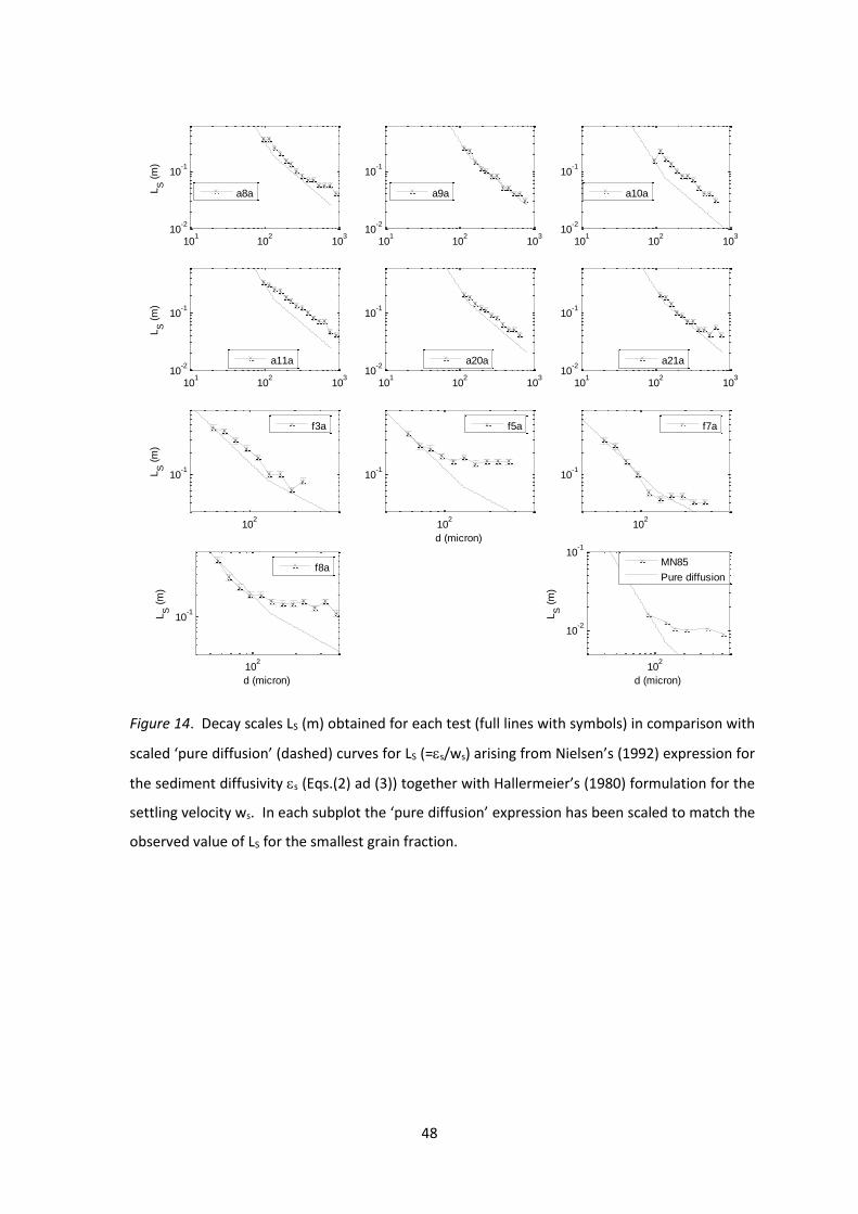
48

Figure 14. Decay scales LS (m) obtained for each test (full lines with symbols) in comparison with

scaled ‘pure diffusion’ (dashed) curves for LS (=s/ws) arising from Nielsen’s (1992) expression for

the sediment diffusivity s (Eqs.(2) ad (3)) together with Hallermeier’s (1980) formulation for the

settling velocity ws. In each subplot the ‘pure diffusion’ expression has been scaled to match the

observed value of LS for the smallest grain fraction.

101

102

103

10-2

10-1

LS (

m)

a8a

101

102

103

10-2

10-1

a9a

101

102

103

10-2

10-1

a10a

101

102

103

10-2

10-1

LS (

m)

a11a

101

102

103

10-2

10-1

a20a

101

102

103

10-2

10-1

a21a

102

10-1L

S (

m)

f3a

102

10-1

d (micron)

f5a

102

10-1

f7a

102

10-1

d (micron)

LS (

m)

f8a

102

10-2

10-1

d (micron)

LS (

m)

MN85

Pure diffusion

49

Figure 15. Normalised decay scale LS plotted against X. Figure a) shows results for all the

Deltaflume tests together with the average behaviour of LS/ LST which is indicated by the full

black line. Also included is the laboratory test of MN85. Figure b) repeats the average curve for

LS/ LST and adds a two- part, power law, characterisation showing a ‘diffusive’ behaviour for X<7

and a combined ‘convective + diffusive’ behaviour for X>7.

101

10-1

100

X

LS/L

ST

(a)

101

10-1

100

X

LS/L

ST

(b)

a8a

a9a

a10a

a11a

a20a

a21a

f3a

f5a

f7a

f8a

McFet&Niel

Average

Average

Pure diffusion

Conv + Diff

50

Figure 16. Vertical profiles of d50s the median diameter of the suspended sediment in each

Deltaflume test. The symbols (o) indicate the measured values of d50s and the dashed lines

indicate the median diameter of the respective bed sediment d50b. The predicted empirical fit

(full lines) in each subplot is based on i) the cumulative size distribution for the bed sediment

(Fig. 1), ii) the Transfer function (Eq. (13)) defined according to the distinction made in Eq. (14)

between regular and irregular waves (see Fig. 10) and iii) the decay length scale relationship

given by Eq. (17). In the subplot for test a8a, the black dotted line reproduces the d50s profile

presented for this case by Davies and Thorne (2002) [DT2002].

100 200 300 400

0

0.1

0.2

0.3

0.4

0.5

0.6

Heig

ht

above b

ed z

(m

)

a8a

measured

empirical prediction

d50b

DT2002

100 200 300 400

0

0.1

0.2

0.3

0.4

0.5

0.6

a9a

100 200 300 400

0

0.1

0.2

0.3

0.4

0.5

0.6

a10a

100 200 300 400

0

0.1

0.2

0.3

0.4

0.5

0.6

a11a

100 200 300 400

0

0.1

0.2

0.3

0.4

0.5

0.6

Heig

ht

above b

ed z

(m

)

a20a

100 200 300 400

0

0.1

0.2

0.3

0.4

0.5

0.6

a21a

50 100 150 200

0

0.1

0.2

0.3

0.4

0.5

0.6

d50s

(micron)

Heig

ht

above b

ed z

(m

)

f3a

50 100 150 200

0

0.1

0.2

0.3

0.4

0.5

0.6

d50s

(micron)

f5a

50 100 150 200

0

0.1

0.2

0.3

0.4

0.5

0.6

d50s

(micron)

f7a

50 100 150 200

0

0.1

0.2

0.3

0.4

0.5

0.6

d50s

(micron)

f8a

51

Appendix A

C-profile for constant + linear diffusivity

Thorne et al. (2002) compared total C-profiles (i.e. the sum of all fractions), obtained using an

acoustic backscatter system, ABS, in the Deltaflume, above the medium sand bed with Nielsen’s

(1992) ‘convection-diffusion’ and ‘pure convection’ profiles. The latter solution, which is of power

law type, arises from consideration of the probability of a particle being entrained to a defined

height above the bed. They found that both profile types could be tuned to give good agreement

with the ABS data and considered the sediment diffusivity profile that was implied by treating the

‘pure convection’ profile as a solution of the sediment diffusion equation. The resulting sediment

diffusivity profile turned out to have a ‘constant + linear’ nature. In a model intercomparison with C-

profile data, such a profile was found by Sistermans (2002) to be both the optimum one for waves +

current above a rippled bed and also as good as a height-constant profile for waves alone above

ripples. A critical consideration in each case was that, in the rippled regime, the s profile should not

tend to zero on approaching the bed.

The analysis in the present paper has focussed on interpretations involving a height-constant

sediment diffusivity s and the corresponding exponential C-profile shape. At the same time it has

been apparent that a minority of the individual C-profiles (for individual fractions within a test) are

better described by a linearly height-varying diffusivity corresponding to a power law profile. With

the steady state diffusion equation given by Eq.(1):

𝑠𝑑𝐶

𝑑𝑧+ 𝑤𝑠𝐶 = 0 (A.1)

it is potentially relevant therefore to consider a sediment diffusivity having the assumed form:

𝑠 = 𝑎 + 𝑏𝑧 (A.2)

where parameters a and b are independent of height z above the bed. [As noted in §1, for rippled

and very rough beds in a wave-induced flow, it can be assumed that, e.g., a = 0.016U1k

s , b = 0 and,

for flat rough beds, e.g., a = 0, b = u*w

.]

The solution of Eq.(A.1) subject to (A.2) is simply:

𝐶 = (𝑎 + 𝑏𝑧)−𝑤𝑠 𝑏⁄ + 𝑐𝑜𝑛𝑠𝑡𝑎𝑛𝑡 (A.3)

and, taking the boundary condition C=Cr at z=z

r it follows that:

𝐶

𝐶𝑟= (

𝑎+𝑏𝑧𝑟

𝑎+𝑏𝑧)

𝑤𝑠 𝑏⁄

(A.4)

This solution reverts to the usual Rouse-type power law (c.f. Eq.(7)) in the limit a0 :

52

𝑐

𝑐𝑟= (

𝑧𝑟

𝑧)

𝑤𝑠 𝑏⁄

(A.5)

while, in the limit b0, an exponential profile (c.f. Eq.(5)) is recovered, the formal limiting process

being more involved in this case:

𝐶 = 𝐶𝑟𝑒−𝑧 𝐿𝑆⁄ (A.6)

where LS =a/ws.

In a simple schematised way, one can illustrate the change from a power law to exponential law C-

profile by changing the ratio a:b. In the illustrative example in Figure A.1, a=[0 0.4 1 2.5] and b=[5 2

1 0.5] giving the 4 (dimensional) quotients a/b shown in the legend, together with the exponential

profile case for which a/b is infinite. Figure A.1a shows a linear plot of the 5 profiles each of which

takes value unity at the level zref

. The same curves are plotted in Figure A.1b in a log-log plot. The

power law (a/b=0) becomes a straight line while other curves for non-zero values ‘a’ of become

strongly curved. In Figure A.1c the curves are next plotted using log-linear axes. Now the

exponential curve (a/b=) is a straight line, while the remaining curves become curved in the

opposite sense. It is evident that fairly straight lines are found in this plot for the wide range of

values having a/b > 1. This latter point might help to explain why the exponential fitting method

works well for most of the C-profile fractions in most of the tests in the Deltaflume, and why

Sistermans (2002) found that several different possible functional forms for s that he considered

gave roughly similar C-profile shapes.

Appendix B

Nielsen’s (1992) ‘selective entrainment’ concept interpreted as a Transfer function

As noted in §2.1 Nielsen (1992, §5.3.7 ) commented on the lack of information available about the

selective entrainment of different sand sizes under waves and suggested the simple formula:

𝑓𝑟𝑎𝑐𝑡𝑖𝑜𝑛 𝑖𝑛 𝑏𝑒𝑑

𝑓𝑟𝑎𝑐𝑡𝑖𝑜𝑛 𝑖𝑛 𝑛𝑒𝑎𝑟 𝑏𝑒𝑑 𝑠𝑢𝑠𝑝𝑒𝑛𝑠𝑖𝑜𝑛≈

𝑑

𝑑50𝑏 (B.1)

This approach, which is included for comparison in Figure 6, was based on a limited amount of

graded-sediment data obtained for the very rough / rippled turbulent regime rippled beds under

waves, including both field data (RE=(2.6-5.0)105, A1/ks=1.7-3.5, see Nielsen, 1983) and also the

laboratory data of MN85 (RE=0.11105, A1/ks=1.5). In practice, the linear dependence on d/d50b of

the quotient on the left hand side of Eq.(B.1) will only provide a reasonable description of the

53

entrainment process up to the point where the sediment capable of being put into suspension is

exhausted. A departure from the linear dependence necessarily then occurs, as is evident in

Nielsen’s (1992) Figure 5.3.6 for the largest grain fraction in the experiment of MN85. For the

Deltaflume tests a pronounced departure from the linear behaviour occurs for d/d50b 1 for the fine

sand and 1.5 for the medium sand (figure not shown). Figure B.1 shows the Transfer functions,

defined by Eq. (13), consequent upon the use of Eq.( B.1) for both the fine and medium sand bed

distributions in the Deltaflume and also for the fine sand used in the experiment of MN85. The

functional form for Tr in each case is qualitatively similar to the results plotted in Figure 8, but the

variation exhibited by the individual tests in each group is absent. More importantly, the magnitudes

of the Transfer functions based on the selective entrainment argument become progressively larger

than observed as d/d50b increases, as a result of the breakdown of Eq.(B.1) for the larger fractions.

This bias is seen for all of the Deltaflume tests and also for the test of MN85 for which the observed

Tr values in Figure 8 are 0.1 for the largest fractions, but are 0.3 from use of Eq.(B.1). The

preference in the present paper for the use of the functional form for Tr given by Eq.(13), rather

than a form like Eq.(B.1) or a fractional reference concentration approach, arises from both the

limitations of the latter equation and also the present emphasis on the behaviour of the coarser

fractions which is best analysed using a description like Eq.(13)

Appendix C

Hallermeier’s (1981) settling velocity formulation

The formulation is expressed here for a single natural sand grain of diameter d settling in still water,

rather than as the median diameter in Hallermeier’s paper. The Reynolds number of the settling

grain is given by

dws

s Re (C.1)

and the Archimedes Buoyancy Index, which is related to the dimensionless grain size D, by:

2

3

3

*

gdDA s

(C.2)

where = kinematic viscosity, g = acceleration due to gravity and s, = sediment, fluid density. The settling velocity ws is obtained from the following equations for the respective regimes:

54

][101005.1

][10396

][3918

Re

645.0

47.0

regimeTurbulentAforA

regimealTransitionAforA

regimeStokesAforA

dwss

(C.3)

For natural sand grains settling in fresh water (s/=2.65, =1 mm2/s, g=9810 mm/s2) the transitional

regime corresponds to the grain size range [134,851] micron.

Appendix D

Determination of the profile of the median diameter of the suspended sediment d50s

The method used in §7 involved the following steps for each test:

1. The appropriate bed sediment size distribution in Figure 1 was interpolated using 100 intervals of

10 m for the medium sand and 5 m for the fine sand. The grain diameter attributed to each

interval was the central size for that interval.

2. The Transfer function (Eq.(14)) was used to convert the bed size distribution into a cumulative

distribution for the reference concentration using the 100 defined grain size intervals. The ripple

dimensions (,) were taken from Table 1, together with the appropriate value of d50b and

coefficients (b1,b2) appropriate for regular/irregular waves for use in Eq.(14).

3. The cumulative reference concentration curve was discretized into individual reference

concentration values corresponding to the 100 grain size intervals.

4. The total decay length scale LST was determined based on the scheme shown in Figure 12.

5. For each grain size d the value of decay scale LS was determined using Eq.(17) with coefficient c4

defined according to the value of X.

6. Using the set of reference concentrations and corresponding LS values, concentration profiles

Ci(zj) were determined for each of the 100 grain sizes (i) at a set of 100 heights (j) above the crest,

from z = 0 to 1m with an interval of 0.01m.

7. At each height j, the 100 concentration values for each test were summed to give the total

concentration Csum(zj).

8. The cumulative concentration Ccum,i(zj) at each height zj was determined and normalised by the

value Csum(zj).

55

9. Finally, from the resulting quotient Ccum,i(zj)/Csum(zj) the values of d50s(zj) were determined by

interpolation among the sizes to yield the ‘50% finer than’ size value.

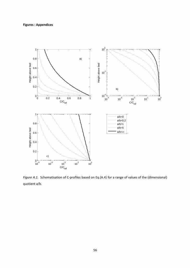
56

Figures : Appendices

Figure A.1. Schematisation of C-profiles based on Eq.(A.4) for a range of values of the (dimensional)

quotient a/b.

0 0.2 0.4 0.6 0.8 10

0.2

0.4

0.6

0.8

1

C/Cref

Heig

ht

above b

ed

a)

10-4

10-3

10-2

10-1

100

10-2

10-1

100

C/Cref

Heig

ht

above b

ed

b)

10-4

10-3

10-2

10-1

100

0

0.2

0.4

0.6

0.8

1

C/Cref

Heig

ht

above b

ed

c)

a/b=0

a/b=0.2

a/b=1

a/b=5

a/b=

57

Figure B.1. Transfer functions calculated on the basis of Nielsen’s (1992) ‘selective entrainment’

function (Eq.(B.1)) for the fine and medium sand beds in the Deltaflume and also the fine sand bed

used in the experiment of MN85. The calculations have been made by i) converting the cumulative

bed grain size distributions shown in Figure 1 into 20 separate fractions, ii) applying Eq.(B.1) to each

fraction, iii) calculating the resulting cumulative size distributions of the reference concentration (c.f.

Figure 7), and iv) using Eq.(13) to determine the respective Transfer functions shown in this figure.

While the results are qualitatively similar to those in Figure 8, they do not discriminate between

different test conditions and, importantly, exhibit bias to relatively larger Tr values than observed,

particularly for the larger grain fractions within each Deltaflume grouping.

0 100 200 300 400 500 600 700 800 900 10000

0.2

0.4

0.6

0.8

1

d (micron)

Tra

nsfe

r fu

nction

Nielsen (1992) Selective entrainment function as a Transfer function

medium

fine

fine: MN85