on vertex identifying codes for infinite...
TRANSCRIPT

Iowa State UniversityDigital Repository @ Iowa State University
Graduate Theses and Dissertations Graduate College
2011
On Vertex Identifying Codes For Infinite LatticesBrendon StantonIowa State University
Follow this and additional works at: http://lib.dr.iastate.edu/etdPart of the Mathematics Commons
This Dissertation is brought to you for free and open access by the Graduate College at Digital Repository @ Iowa State University. It has been acceptedfor inclusion in Graduate Theses and Dissertations by an authorized administrator of Digital Repository @ Iowa State University. For moreinformation, please contact [email protected].
Recommended CitationStanton, Brendon, "On Vertex Identifying Codes For Infinite Lattices" (2011). Graduate Theses and Dissertations. Paper 12019.
On Vertex Identifying Codes For Infinite Lattices
by
Brendon Michael Stanton
A dissertation submitted to the graduate faculty
in partial fulfillment of the requirements for the degree of
DOCTOR OF PHILOSOPHY
Program of Study Committee:Ryan Martin, Major Professor
Maria AxenovichClifford Bergman
Leslie HogbenChong Wang
Iowa State University
Ames, Iowa
2011

ii
DEDICATION
I would like to dedicate this thesis to my parents. Without their love and support, I never
would have made it this far. I would also like to thank all of my friends, family, teachers and
professors who have helped me through my many years of education.

iii
TABLE OF CONTENTS
LIST OF FIGURES . . . . . . . . . . . . . . . . . . . . . . . . . . . . . . . . . . v
CHAPTER 1. GENERAL INTRODUCTION . . . . . . . . . . . . . . . . . . 1
1.1 Thesis Organization . . . . . . . . . . . . . . . . . . . . . . . . . . . . . . . . . 1
1.2 Definitions . . . . . . . . . . . . . . . . . . . . . . . . . . . . . . . . . . . . . . . 2
1.3 Literature Review . . . . . . . . . . . . . . . . . . . . . . . . . . . . . . . . . . 3
1.3.1 General Bounds and Constructions . . . . . . . . . . . . . . . . . . . . . 3
1.3.2 Codes and Infinite Graphs . . . . . . . . . . . . . . . . . . . . . . . . . . 7
1.3.3 Variants of r-Identifying Codes . . . . . . . . . . . . . . . . . . . . . . . 12
CHAPTER 2. LOWER BOUNDS FOR IDENTIFYING CODES IN SOME
INFINITE GRIDS . . . . . . . . . . . . . . . . . . . . . . . . . . . . . . . . . 15
Abstract . . . . . . . . . . . . . . . . . . . . . . . . . . . . . . . . . . . . . . . . . . . 15
2.1 Introduction . . . . . . . . . . . . . . . . . . . . . . . . . . . . . . . . . . . . . . 15
2.2 Definitions and General Lemmas . . . . . . . . . . . . . . . . . . . . . . . . . . 17
2.3 Lower Bound for the Hexagonal Grid . . . . . . . . . . . . . . . . . . . . . . . . 20
2.4 Lower Bounds for the Square Grid . . . . . . . . . . . . . . . . . . . . . . . . . 21
2.5 Conclusions . . . . . . . . . . . . . . . . . . . . . . . . . . . . . . . . . . . . . . 32
CHAPTER 3. IMPROVED BOUNDS FOR r-IDENTIFYING CODES OF
THE HEX GRID . . . . . . . . . . . . . . . . . . . . . . . . . . . . . . . . . . 34
Abstract . . . . . . . . . . . . . . . . . . . . . . . . . . . . . . . . . . . . . . . . . . . 34
3.1 Introduction . . . . . . . . . . . . . . . . . . . . . . . . . . . . . . . . . . . . . . 34
3.2 Construction and Definitions . . . . . . . . . . . . . . . . . . . . . . . . . . . . 36
3.3 Distance Claims . . . . . . . . . . . . . . . . . . . . . . . . . . . . . . . . . . . 37
iv
3.4 Proof of Main Theorem . . . . . . . . . . . . . . . . . . . . . . . . . . . . . . . 39
3.5 Proof of Lemmas . . . . . . . . . . . . . . . . . . . . . . . . . . . . . . . . . . . 46
3.6 Conclusion . . . . . . . . . . . . . . . . . . . . . . . . . . . . . . . . . . . . . . 49
Acknowledgment . . . . . . . . . . . . . . . . . . . . . . . . . . . . . . . . . . . . . . 50
CHAPTER 4. VERTEX IDENTIFYING CODES FOR THE n-DIMENSIONAL
LATTICE . . . . . . . . . . . . . . . . . . . . . . . . . . . . . . . . . . . . . . 51
Abstract . . . . . . . . . . . . . . . . . . . . . . . . . . . . . . . . . . . . . . . . . . . 51
4.1 Introduction . . . . . . . . . . . . . . . . . . . . . . . . . . . . . . . . . . . . . . 51
4.2 Definitions . . . . . . . . . . . . . . . . . . . . . . . . . . . . . . . . . . . . . . . 53
4.3 Using Dominating Sets for Constructions when r = 1 . . . . . . . . . . . . . . . 54
4.4 A Monotonicity Theorem . . . . . . . . . . . . . . . . . . . . . . . . . . . . . . 56
4.5 The 4-dimensional case . . . . . . . . . . . . . . . . . . . . . . . . . . . . . . . . 57
4.6 General Bounds and Construction . . . . . . . . . . . . . . . . . . . . . . . . . 60
4.7 Conclusions . . . . . . . . . . . . . . . . . . . . . . . . . . . . . . . . . . . . . . 65
4.8 Acknowledgements . . . . . . . . . . . . . . . . . . . . . . . . . . . . . . . . . . 66
CHAPTER 5. ADDENDUM TO “LOWER BOUNDS FOR IDENTIFY-
ING CODES IN SOME INFINITE GRIDS” AND ANOTHER RESULT 67
5.1 Proof of Theorem 2.4 . . . . . . . . . . . . . . . . . . . . . . . . . . . . . . . . . 67
5.2 A Lower Bound for (r,≤ 2)-Identifying Codes . . . . . . . . . . . . . . . . . . . 74
CHAPTER 6. VERTEX IDENTIFYING CODES FOR REGULAR GRAPHS 77
6.1 Introduction . . . . . . . . . . . . . . . . . . . . . . . . . . . . . . . . . . . . . . 77
6.2 Theorems . . . . . . . . . . . . . . . . . . . . . . . . . . . . . . . . . . . . . . . 77
6.3 Proofs . . . . . . . . . . . . . . . . . . . . . . . . . . . . . . . . . . . . . . . . . 77
6.4 Construction of Graphs Satisfying the Bounds . . . . . . . . . . . . . . . . . . . 81
BIBLIOGRAPHY . . . . . . . . . . . . . . . . . . . . . . . . . . . . . . . . . . . 86

v
LIST OF FIGURES
1.1 An optimal identifying code for the 3-dimensional lattice (partial) . . . 11
2.1 The sets S1, S2, S3 and S4 surrounding a codeword in the square grid 22
2.2 A proof by picture that p(c) ≤ 8 when |I2(c)| = 2 in the square grid . . 22
2.3 A right angle of witnesses in the square grid (1 of 2) . . . . . . . . . . 23
2.4 A right angle of witnesses in the square grid (2 of 2) . . . . . . . . . . 24
2.5 A type 1 codeword in the square grid . . . . . . . . . . . . . . . . . . . 26
2.6 A type 2 codeword in the square grid . . . . . . . . . . . . . . . . . . . 26
2.7 A type 3 codeword in the square grid . . . . . . . . . . . . . . . . . . . 27
2.8 An 8-pair codeword with |I2(c)| = 2 in the square grid . . . . . . . . . 28
2.9 An 8-pair codeword with |I2(c)| = 1 in the square grid . . . . . . . . . 30
3.1 An r-identifying code in the hexagonal grid for r = 6. . . . . . . . . . . 36
3.2 An r-identifying code in the hexagonal grid for r = 7. . . . . . . . . . . 37
4.1 A table of bounds of densities of codes for small values of n. . . . . . . 52
4.2 A table of bounds for the size of a dominating set on Hn. . . . . . . . 56
5.1 A ball of radius 3 in the hexagonal grid (1 of 3) . . . . . . . . . . . . . 68
5.2 A ball of radius 3 in the hexagonal grid (2 of 3) . . . . . . . . . . . . . 69
5.3 A ball of radius 3 in the hexagonal grid (3 of 3) . . . . . . . . . . . . . 70

1
CHAPTER 1. GENERAL INTRODUCTION
Vertex identifying codes were first introduced by Karpovsky, Chakrabarty and Levitin [29]
in 1998 as a way to help with fault diagnosis in multiprocessor computer systems. Since then,
study of these codes and their variants have exploded. Antoine Lobstein maintains an internet
bibliography [33] which at the time of this writing, contains nearly 200 articles on the subject.
Since the size of a code depends largely on topology of the particular graph, it is common
to restrict our study of codes to various graphs and classes of graphs. The main focus of this
thesis is on the primary variant of these codes–called r-identifying codes–and their densities
on various locally finite infinite graphs, all of which have a representation on a lattice.
1.1 Thesis Organization
The thesis is organized as follows:
In Chapter 1 the main ideas are described and a review of the literature on the subject is
given.
Chapter 2 presents the paper “Lower Bounds for Identifying Codes in Some Infinite Grids” [34]
published in Electronic Journal of Combinatorics. This paper, co-written with Ryan Martin,
finds lower bounds for 2-identifying codes for the square and hexagonal grids by way of a
counting argument. In addition, the paper makes use of the discharging method to further
increase the lower bound for the square grid. The technique presented here can be extended to
provide lower bounds for other grids and other values of r. However, it does not give bounds
that are as good as the current best known lower bounds in most cases. One exception is the
case r = 3 for the hexagonal grid, which is given in Chapter 5.
Chapter 3 presents the paper “Improved Bounds for r-Identifying Codes of the Hex Grid” [38]
2
published in SIAM Journal on Discrete Mathematics. By contrast to [34] which provides lower
bounds, this paper provides general constructions of codes for the hexagonal grid which de-
crease the upper bounds of the minimum densities of r-identifying codes for large values of
r.
Chapter 4 presents the paper “Vertex Identifying Codes for the n-dimensional Lattice” [39]
submitted for publication to Discrete Mathematics. Here we look at the n-dimensional analogue
of the square grid and provide a general overview and discussion of codes on the n-dimensional
lattice, providing both upper and lower bounds for r-identifying codes in both the most general
case (r-identifying codes for the n-dimensional lattice) and in more specific cases such as the
case when r = 1 and even more specifically when n = 4.
Chapter 5 ties up some loose ends, providing a proof that was promised in “Lower Bounds
for Identifying Codes in Some Infinite Grids”[34] as well as another result which has not yet
been submitted for publication.
Chapter 6 is part of a work in progress with Ryan Martin. It addresses the general issue of
codes on (finite) regular graphs–improving upon the general lower bound given in Theorem 1.12
and providing constructions of graphs that attain these bounds.
1.2 Definitions
We must first begin with some basic definitions in order to introduce the notion of a vertex
identifying code. For basic definitions about graph theory, we refer the reader to “Introduction
to Graph Theory” [40] by Doug West.
Definition 1.1. Given a graph G, the distance between two vertices u, v is written d(u, v)
which is the length of the shortest path between u and v.
Definition 1.2. Given a graph G, the ball of radius r, centered at v, denoted by Br(v) is
defined as:
Br(v) = {u : d(u, v) ≤ r}.
Definition 1.3. Given a graph G, a code C is a nonempty subset of V (G). The elements of
C are called codewords.

3
Although the above definition may seem a bit unnecessary, it is useful when writing proofs
involving identifying codes. If trying to prove that some set C is an r-identifying code (or some
other type of identifying code), it is often useful to refer to C as a code, which we can simply
refer to it as a code without having to worry about whether or not it has the r-identifying
property.
Definition 1.4. Given a graph G and a code C, the r-identifying set (or simply identifying
set) of a vertex v, is defined as
Ir(v) = Ir(v, C) = Br(v) ∩ C.
This brings us to the main definition.
Definition 1.5. Given a graph G, a code C is called r-identifying if for each distinct u, v ∈
V (G) we have
1. Ir(v) 6= ∅ and
2. Ir(u) 6= Ir(v).
When r = 1, we simply refer to C as an identifying code.
The idea behind an r-identifying code is that given an identifying set Ir(v) and a code C,
we should be able to determine what v is just from its identifying set. The motivation for this
definition is that if we are given a multiprocessor system, we wish to be able to determine when
an error occurred by communicating with only a subset of the processors. If there is no error,
then no processors report back that there was an error. Hence, the first condition ensures that
at least 1 processor will report back if there is an error. The second condition ensures that we
are able to determine the source of the error.
1.3 Literature Review
1.3.1 General Bounds and Constructions
Karpovsky, Chakrabarty and Levitin [29] were the first to introduce the notion of an
identifying code. They provided many basic constructions and bounds for the size of codes–

4
many of which are still best known for some graphs. First though, we note that not all graphs
have codes. For instance, Kn–the complete graph on n vertices–does not allow an r-identifying
code. In the following theorem from folklore, we present some equivalent conditions for the
existence of a code:
Theorem 1.6. For any graph G, the following are equivalent:
1. G has an r-identifying code;
2. V (G) is an r-identifying code; and
3. Br(u) 6= Br(v) for all distinct u, v ∈ V (G).
Proof. (2) ⇒ (1) is trivial. It is also relatively easy to see that (2) ⇔ (3). Suppose that V (G)
is a code for G. Then for all u 6= v we have Br(u) ∩ V (G) 6= Br(v) ∩ V (G) by definition of a
code and so Br(u) 6= Br(v). Likewise, if V (G) is not a code, it must be the case that for some
u, v ∈ V (G) with u 6= v we have Br(u) ∩ V (G) = Br(v) ∩ V (G) and so Br(u) = Br(v).
Finally, to show (1) ⇒ (2) we need a lemma.
Lemma 1.7. Let C be an r-identifying code for a graph G. Then for any S ⊂ V (G) C ∪ S is
an r-identifying code for G.
The proof of the lemma is just an exercise in basic set theory. Since C is a code, we have
Br(v) ∩ C 6= ∅ for each v ∈ V (G). Then by De Morgan’s law, we have
Br(v) ∩ (C ∪ S) = (Br(v) ∩ C) ∪ (Br(v) ∩ S) ⊂ Br(v) ∩ C 6= ∅.
This shows that C ∪ S has condition (1) from Definition 1.16. To show it also has the second
condition, for any distinct u, v ∈ V (G), there must be some codeword in one identifying set
that isn’t in the other. Without loss of generality, assume that c ∈ Br(v)∩C but c 6∈ Br(u)∩C.
Again by De Morgan we have c ∈ Br(v) ∩ (C ∪ S). However, c ∈ Br(v) and c ∈ C. Since
c 6∈ Br(v)∩C, then c 6∈ Br(v). Thus, c 6∈ Br(v)∩ (C ∪ S), completing the proof of our lemma.
Using this lemma, it now follows that if G has a code C, then take S = V (G) and we have
C ∪ V (G) = V (G) is a code for G, completing the proof.
5
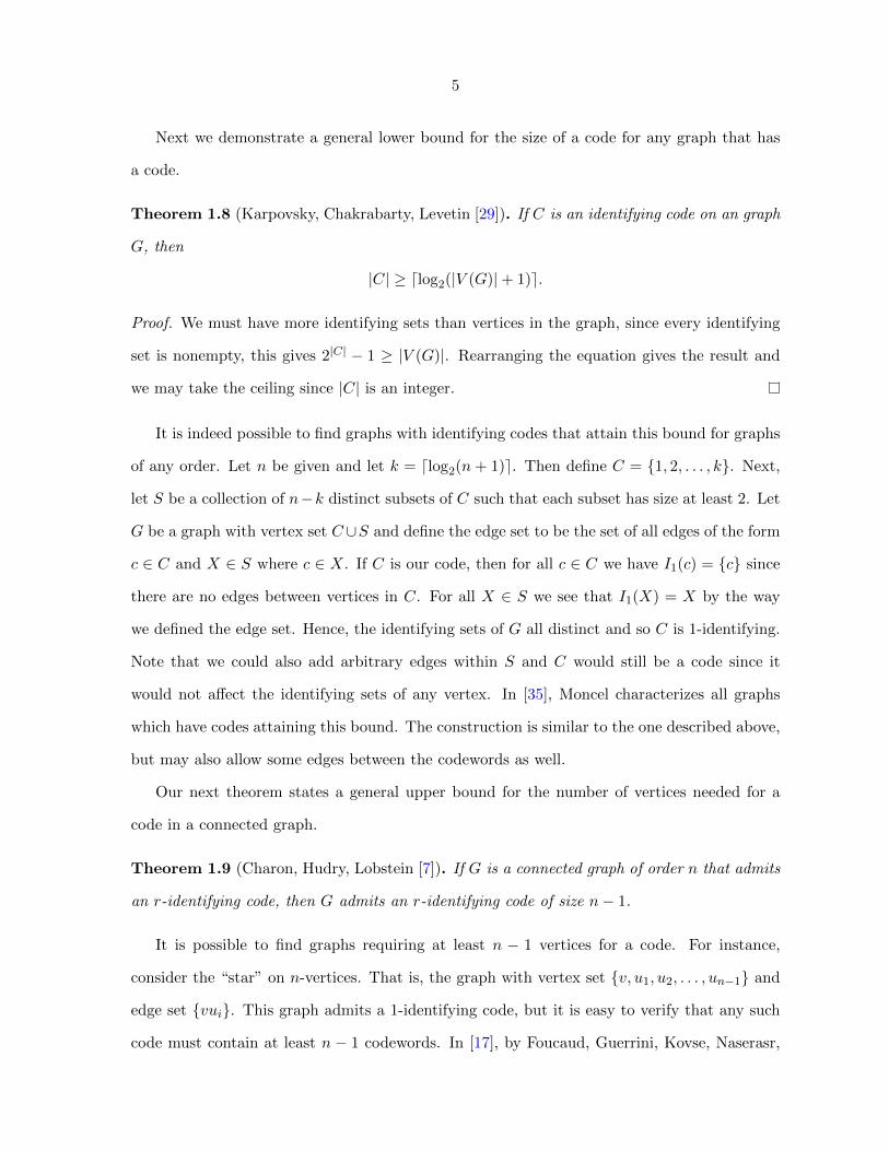
Next we demonstrate a general lower bound for the size of a code for any graph that has
a code.
Theorem 1.8 (Karpovsky, Chakrabarty, Levetin [29]). If C is an identifying code on an graph
G, then
|C| ≥ dlog2(|V (G)|+ 1)e.
Proof. We must have more identifying sets than vertices in the graph, since every identifying
set is nonempty, this gives 2|C| − 1 ≥ |V (G)|. Rearranging the equation gives the result and
we may take the ceiling since |C| is an integer.
It is indeed possible to find graphs with identifying codes that attain this bound for graphs
of any order. Let n be given and let k = dlog2(n + 1)e. Then define C = {1, 2, . . . , k}. Next,
let S be a collection of n−k distinct subsets of C such that each subset has size at least 2. Let
G be a graph with vertex set C∪S and define the edge set to be the set of all edges of the form
c ∈ C and X ∈ S where c ∈ X. If C is our code, then for all c ∈ C we have I1(c) = {c} since
there are no edges between vertices in C. For all X ∈ S we see that I1(X) = X by the way
we defined the edge set. Hence, the identifying sets of G all distinct and so C is 1-identifying.
Note that we could also add arbitrary edges within S and C would still be a code since it
would not affect the identifying sets of any vertex. In [35], Moncel characterizes all graphs
which have codes attaining this bound. The construction is similar to the one described above,
but may also allow some edges between the codewords as well.
Our next theorem states a general upper bound for the number of vertices needed for a
code in a connected graph.
Theorem 1.9 (Charon, Hudry, Lobstein [7]). If G is a connected graph of order n that admits
an r-identifying code, then G admits an r-identifying code of size n− 1.
It is possible to find graphs requiring at least n − 1 vertices for a code. For instance,
consider the “star” on n-vertices. That is, the graph with vertex set {v, u1, u2, . . . , un−1} and
edge set {vui}. This graph admits a 1-identifying code, but it is easy to verify that any such
code must contain at least n − 1 codewords. In [17], by Foucaud, Guerrini, Kovse, Naserasr,

6
Parreau, and Valicov, all graphs admitting a minimum code of size n− 1 are characterized. In
another paper, Charon, Hudry and Lobstein take this idea even further.
Theorem 1.10 (Charon, Hudry, Lobstein [6]). For every integer r ≥ 1 and a integer n
sufficiently large with respect to r, that for every integer k in the interval [dlog2(n+ 1)e, n− 1],
there is a graph G that admits a minimum r-identifying code of size k.
Since we can find graph with codes of basically any size, we usually desire to impose some
sort of structure on our graph in order to get any meaningful result. One useful way to do this
is to impose some sort of regularity condition on our graph.
Theorem 1.11 (Karpovsky, Chakrabarty, Levetin [29]). If C is an r-identifying code for a
graph G of order n and for each vertex v ∈ V (G) we have |Br(v)| ≤ br, then
|C| ≥ 2n
br + 1.
Proof. Let C = {c1, c2, . . . , ck}. We start by summing the size of the identifying sets.
∑v∈V (G)
|Ir(v)|.
On the other hand, for each cj , we have cj ∈ Ir(vi) for exactly |Br(cj)| distinct values of i.
Hence, we havek∑
j=1
|Br(cj)| =∑
v∈V (G)
|Ir(v)|.
However, since |Br(v)| = br for any vertex, this gives
br|C| =∑
v∈V (G)
|Ir(v)|.
Now we see that there can be at most |C| identifying sets of size 1 and all the rest must have
size at least 2. This gives a lower bound for the right hand side
br|C| ≥ |C|+ 2(n− |C|).
Rearranging the inequality gives the desired result.
In particular, this gives a bound for identifying codes of regular graphs.
7
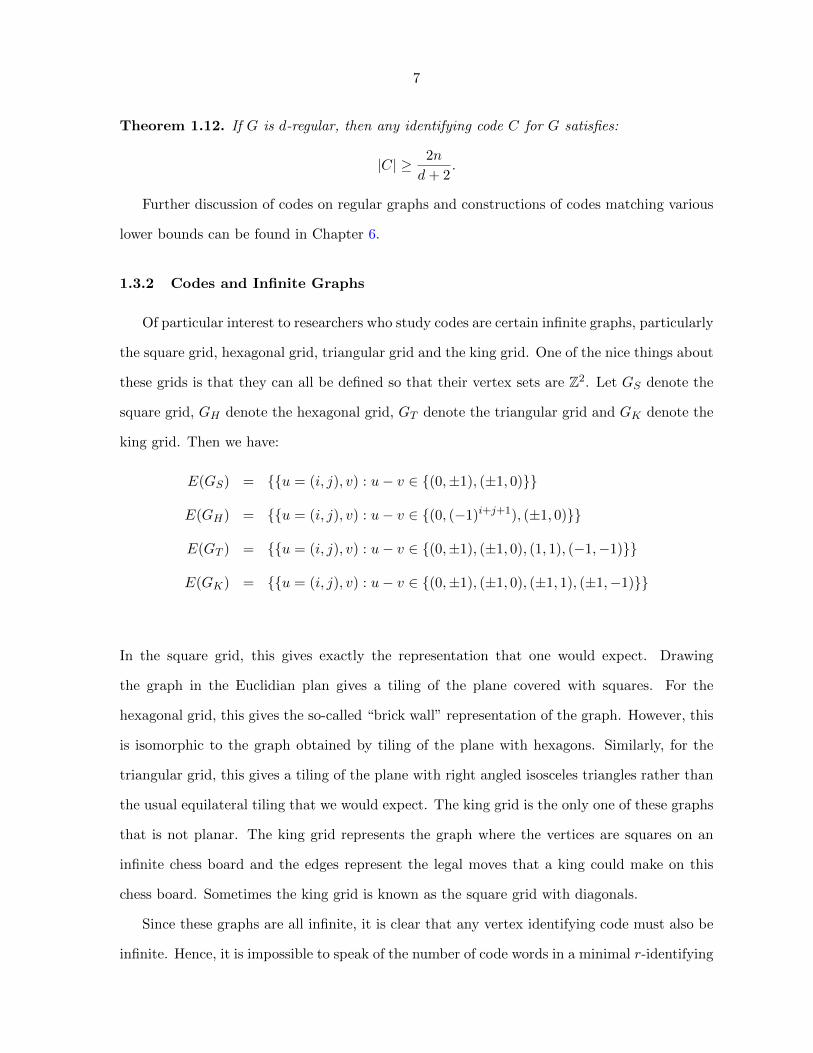
Theorem 1.12. If G is d-regular, then any identifying code C for G satisfies:
|C| ≥ 2n
d+ 2.
Further discussion of codes on regular graphs and constructions of codes matching various
lower bounds can be found in Chapter 6.
1.3.2 Codes and Infinite Graphs
Of particular interest to researchers who study codes are certain infinite graphs, particularly
the square grid, hexagonal grid, triangular grid and the king grid. One of the nice things about
these grids is that they can all be defined so that their vertex sets are Z2. Let GS denote the
square grid, GH denote the hexagonal grid, GT denote the triangular grid and GK denote the
king grid. Then we have:
E(GS) = {{u = (i, j), v) : u− v ∈ {(0,±1), (±1, 0)}}
E(GH) = {{u = (i, j), v) : u− v ∈ {(0, (−1)i+j+1), (±1, 0)}}
E(GT ) = {{u = (i, j), v) : u− v ∈ {(0,±1), (±1, 0), (1, 1), (−1,−1)}}
E(GK) = {{u = (i, j), v) : u− v ∈ {(0,±1), (±1, 0), (±1, 1), (±1,−1)}}
In the square grid, this gives exactly the representation that one would expect. Drawing
the graph in the Euclidian plan gives a tiling of the plane covered with squares. For the
hexagonal grid, this gives the so-called “brick wall” representation of the graph. However, this
is isomorphic to the graph obtained by tiling of the plane with hexagons. Similarly, for the
triangular grid, this gives a tiling of the plane with right angled isosceles triangles rather than
the usual equilateral tiling that we would expect. The king grid is the only one of these graphs
that is not planar. The king grid represents the graph where the vertices are squares on an
infinite chess board and the edges represent the legal moves that a king could make on this
chess board. Sometimes the king grid is known as the square grid with diagonals.
Since these graphs are all infinite, it is clear that any vertex identifying code must also be
infinite. Hence, it is impossible to speak of the number of code words in a minimal r-identifying
8
code. Thus we usually like to speak of the density of a code on one of these graphs. Roughly
speaking, this is the proportion of vertices in the graph that are codewords. However, this
definition doesn’t have a precise mathematical meaning. In practice, any reasonable way of
counting the density of a code will give the correct density, however, we still need a definition
for this to be precise. Let Qm = [−m,m]× [−m,m].
Definition 1.13. The density of a code C for the square, triangular, hexagonal and king grids
is
D(C) = lim supm→∞
|C ∩Qm||Qm|
.
In Chapter 4 we extend this definition to graphs whose vertex set is Zn.
This definition is analogous to how we would define the density of a code on a finite graph
G (i.e. D(C) = |C|/|V (G)|). In fact, Theorem 1.11 and Theorem 1.12 extend to infinite graphs
as well, as we see below..
1.3.2.1 1-Identifying Codes for Infinite Graphs
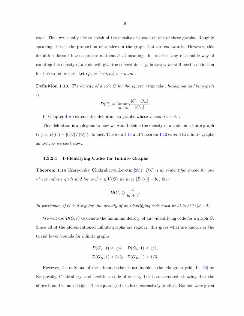
Theorem 1.14 (Karpovsky, Chakrabarty, Levetin [29]). If C is an r-identifying code for one
of our infinite grids and for each v ∈ V (G) we have |Br(v)| = br, then
D(C) ≥ 2
br + 1.
In particular, if G is d-regular, the density of an identifying code must be at least 2/(d+ 2).
We will use D(G, r) to denote the minimum density of an r-identifying code for a graph G.
Since all of the aforementioned infinite graphs are regular, this gives what are known as the
trivial lower bounds for infinite graphs:
D(GT , 1) ≥ 1/4; D(GS , 1) ≥ 1/3;
D(GH , 1) ≥ 2/5; D(GK , 1) ≥ 1/5.
However, the only one of these bounds that is attainable is the triangular grid. In [29] by
Karpovsky, Chakrabary, and Levitin a code of density 1/4 is constructed, showing that the
above bound is indeed tight. The square grid has been extensively studied. Bounds were given

9
by Cohen, Honkala, Lobstein, and Zemor [9], Cohen, Honkala, Mollard, Gravier, Lobstien,
Payan, and Zemor [11] and Karpovsky, Chakrabarty and Levitin [29] before it was shown by
Ben-Haim and Litsyn [1] that the D(GS , 1) = 7/20.
It was shown by Cohen, Honkala, Lobstein, and Zemor [12] that D(GK , 1) ≥ 2/9 and in
[3] by Charon, Honkala, Hudry and Lobstein it was shown that this bound was tight. More
generally, it was shown by Charon, Honkala, Hudry and Lobstein [4] that for r ≥ 2 that
D(GK , r) = 1/(4r).
Of all the major grids, only D(GH , 1) remains an open question. In [10] by Cohen, Honkala,
Lobstein, and Zemor, two constructions of density 3/7 are given. In addition, it is shown that
D(GH , 1) ≥ 16/39 which has since been improved to D(GH , 1) ≥ 12/29 in [14]. In addition,
Ari Cukierman and Gexin Yu [15] have reported the existence of at least 3 more identifying
codes of density 3/7, which are non-isomorphic to the ones given in [10] and have also improved
the lower bound to 5/12.
1.3.2.2 r-Identifying Codes for Infinite Graphs
We next wish to turn our attention to the more general r-identifying codes for infinite
graphs, which will be the focus of the majority of this thesis. In general, Theorem 1.12 gives a
very poor lower bound for these densities since br = Θ(r2) (See §5.1 in [5] by Charon, Hudry
and Lobstein). An exception to this is that D(GH , 2) ≥ 2/11, although we improve on this
bound in Chapter 2. In general, however, these lower bounds all have the form Θ(1/r).
We have already addressed the case of the king grid, so we will only mention the bounds for
the hexagonal, square and triangular grids. Most of the bounds in given by Charon, Honkala,
Hudry and Lobstein [3] still stand as the best known general bounds. These bounds are:

10
D(GH , r) ≥
2
5r + 3for r even
2
5r + 2for r odd
D(GS , r) ≥ 3
8r + 4
D(GT , r) ≥ 2
6r + 2.
Other lower bounds for the hexagonal, square and triangular grids were given by Cohen,
Honkala, Lobstein and Zemor [13], Honkala and Lobstein [26] and Cohen, Honkala, Lobstein
and Zemor [13] respectively. In [34], which is Chapter 2, we improve on some of these bounds
for small values of r. Our lower bound D(GH , 2) ≥ 1/5 has since been improved upon by
Junnila and Laihonen [27] where it is shown that D(GH , 2) = 4/19 matching the upper bound
given by Charon, Hudry and Lobstein [5].
For upper bounds, it is usually easiest to find a construction of a code with a given density.
For small values of r, ad hoc constructions are usually best. In particular, Charon, Hudry and
Lobstein [5] used a computer program to find periodic tilings for the triangular grid (2 ≤ r ≤ 6),
square grid (2 ≤ r ≤ 6), and hexagonal grid (2 ≤ r ≤ 30).
There have also been general constructions of codes for arbitrary values of r. In [26],
Honkala and Lobstein show that
D(GS , r) ≤
2
5rfor r even
2r
5r2 − 2r + 1for r odd.
In [3], Charon, Honkala, Hudry and Lobstein show that
D(GT , r) ≤
1
2r + 4for r ≡ 0 (mod 4)
1
2r + 2for r ≡ 1, 2, 3 (mod 4).

11
Also in [3] it is shown that
D(GH , r) ≤
8r − 8
9r2 − 16rfor r ≡ 0 (mod 4)
8
9r − 25for r ≡ 1 (mod 4)
8
9r − 34for r ≡ 2 (mod 4)
8r − 16
(r − 3)(9r − 43)for r ≡ 3 (mod 4) .
In [38], which is the basis of Chapter 3, we improve on this last bound, giving general con-
structions of density
5r + 3
6r(r + 1), if r is even;
5r2 + 10r − 3
(6r − 2)(r + 1)2, if r is odd.
In addition, these improve on the bounds given by Charon, Honkala, Hudry and Lobstein in
[3] for 15 ≤ r ≤ 30, r 6= 17, 21.
Figure 1.1 Part of the code of density 1/4 for the 3-D lattice. Black verticesare codewords.
One other type of infinite graph that is of interest is the n-dimensional lattice (denoted
by Ln), which is the n-dimensional analogue of the square grid. This is defined formally in
12
Section 4.2 of Chapter 4 which is the based on [39].
One particular noteworthy case presented by Karpovsky, Chakrabarty and Levitin [29] is
that D(Ln, 1) = 1/(n+ 1) if and only if n = 2k − 1 for some integer k. For any n, it is known
that 1/(n + 1) is a lower bound for this number, although it is not possible to achieve this
bound in most cases. In Chapter 4 we strive to achieve good asymptotics, showing that the
lower bound is close to the minimum density as well as addressing to more general issue of
r-identifying codes on the n-dimensional lattice.
1.3.3 Variants of r-Identifying Codes
The concept of an identifying code has been generalized in different ways–many of which
are adapted to tackle a real life problem such as sensor networks. Most of these variants will
not be discussed in detail here, but we wish to mention some of them because they have both
practical and mathematical importance.
Perhaps the simplest of these variants is to simply drop condition (1) of Definition 1.16–
that is, we don’t care if one of our vertices has an empty identifying set. Although this doesn’t
have a practical application, it is a natural variant to consider and has been used, for instance
Blass, Honkala, and Litsyn [2], to aid in finding constructions of identifying codes for other
graphs. As it turns out, the lack of this first condition cannot affect the size of a code too
much. Let G be a graph and let Mr(G) be the minimum size of a traditional r-identifying code
for G and let M r(G) denote the minimum size of an identifying code while allowing at most
one empty identifying set.
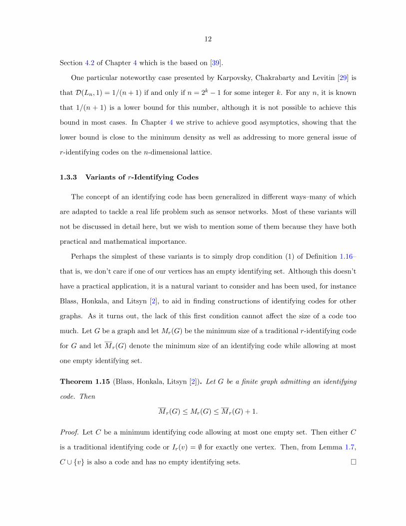
Theorem 1.15 (Blass, Honkala, Litsyn [2]). Let G be a finite graph admitting an identifying
code. Then
M r(G) ≤Mr(G) ≤M r(G) + 1.
Proof. Let C be a minimum identifying code allowing at most one empty set. Then either C
is a traditional identifying code or Ir(v) = ∅ for exactly one vertex. Then, from Lemma 1.7,
C ∪ {v} is also a code and has no empty identifying sets.

13
In addition, this shows that if G is an infinite graph, then the omission of condition (1)
of Definition 1.16 would have no effect on the density of a code since the density of a single
vertex in an infinite graph is 0.
Another variant of an identifying code is to consider a code which not only distinguishes
between individual vertices, but one that is able to distinguish between small subsets of vertices.
If X is a subset of vertices of some graph G and C is a code, then we define
Ir(X) =⋃x∈X
Ir(x).
This brings us to our next definition:
Definition 1.16. Given a graph G, a code C is called (r,≤ `)-identifying if for each distinct
X,Y ⊂ V (G) with |X|, |Y | ≤ ` we have
1. Ir(X) = ∅ iff X = ∅ and
2. Ir(X) 6= Ir(Y ).
Actually, condition (1) can be dropped since I(∅) is necessarily the empty set and by
condition (2) we must have I(∅) 6= I(X) for X 6= ∅. These codes have been well studied, for
instance in Honkala and Laihonen[21, 22, 23], and by Laihonen and Ranto [32]. In section 5.2
we give a lower bound for the minimum density of (r,≤ 2)-identifying codes of the hex grid.
Yet another important variant of identifying codes is the idea of a locating-dominating set.
Originally introduced by Rall and Slater [36], years before the introduction of the concept of
identifying codes, the idea here is that the processors that are marked as codewords are also
able to explicitly communicate when they themselves experience an error. In this case, the
second condition of Definition 1.16 is changed so that we require Ir(u) 6= Ir(v) for u, v 6∈ C.
The flip side to locating dominating codes is the assumption that a faulty processor may
not be able to report if it has experienced an error. These are called strongly identifying codes
and were introduced in [25] by Honkala, Laihonen and Ranto. In this case, we need the sets
{Ir(v), Ir(v) \ {v}} to be disjoint in all cases. These have also been studied in other places, for
instance by Honkala [19] and Laihonen [30].

14
It is easy to see from the definitions that
Strongly Identifying Codes ⊂ Identifying Codes ⊂ Locating-Dominating Sets
and that the inclusions are strict. Every graph admits a locating-dominating set since you
may simply take the entire graph as the locating-dominating set. On the other hand, many
graphs do not admit Identifying codes, the simplest example being Kn–the complete graph on
n vertices. We also see that C4 admits an identifying code, but it is easy to check that it does
not admit a strongly identifying code.
Finally, we will briefly mention some other variants of identifying codes before moving on
to the main part of the thesis. One concept that is commonly studied is to try to find an
identifying code which is still a code if vertices or edges are removed from (or added to) the
graph. This has applications in sensor networks since failures are common and we wish to make
sure we still have a code even if something has failed. These are defined more formally By
Honkala, Karpovsky and Levitin [20] and have been studied in many other papers, for instance
Laihonen [31] and Honkala and Laihonen[24]. Another interesting and recent adaptation of
these codes is to help identify an intruder which was discussed by Roden and Slater [37]. In
addition, the topic of identifying codes on random graphs has been studied by Frieze, Martin,
Moncel, Ruszinko and Smyth [18].

15
CHAPTER 2. LOWER BOUNDS FOR IDENTIFYING CODES IN
SOME INFINITE GRIDS
Based on a paper published in Electronic Journal of Combinatorics
Ryan Martin and Brendon Stanton
Abstract
An r-identifying code on a graph G is a set C ⊂ V (G) such that for every vertex in V (G),
the intersection of the radius-r closed neighborhood with C is nonempty and unique. On a
finite graph, the density of a code is |C|/|V (G)|, which naturally extends to a definition of
density in certain infinite graphs which are locally finite. We present new lower bounds for
densities of codes for some small values of r in both the square and hexagonal grids.
2.1 Introduction
Given a connected, undirected graph G = (V,E), we define Br(v)–called the ball of radius
r centered at v to be
Br(v) = {u ∈ V (G) : d(u, v) ≤ r}.
We call any nonempty subset C of V (G) a code and its elements codewords. A code C is
called r-identifying if it has the properties:
1. Br(v) ∩ C 6= ∅
2. Br(u) ∩ C 6= Br(v) ∩ C, for all u 6= v
16
When C is understood, we define Ir(v) = Ir(v, C) = Br(v) ∩ C. We call Ir(v) the identifying
set of v.
Vertex identifying codes were introduced in [29] as a way to help with fault diagnosis in
multiprocessor computer systems. Codes have been studied in many graphs, but of particular
interest are codes in the infinite triangular, square, and hexagonal lattices as well as the square
lattice with diagonals (king grid). For each of these graphs, there is a characterization so that
the vertex set is Z × Z. Let Qm denote the set of vertices (x, y) ∈ Z × Z with |x| ≤ m and
|y| ≤ m. We may then define the density of a code C by
D(C) = lim supm→∞
|C ∩Qm||Qm|
.
Our first two theorems, Theorem 2.1 and Theorem 2.2, rely on a key lemma, Lemma 2.7,
which gives a lower bound for the density of an r-identifying code assuming that we are able to
show that no codeword appears in “too many” identifying sets of size 2. Theorem 2.1 follows
immediately from Lemma 2.7 and Lemma 2.8 while Theorem 2.2 follows immediately from
Lemma 2.7 and Lemma 2.9.
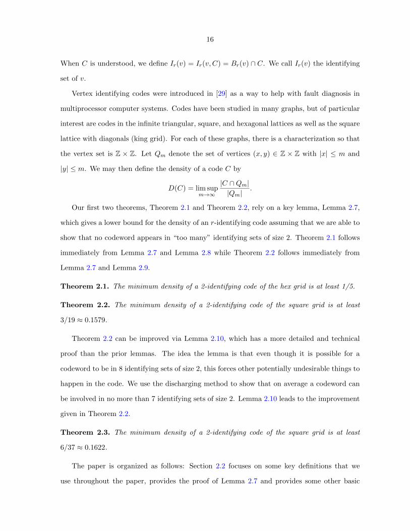
Theorem 2.1. The minimum density of a 2-identifying code of the hex grid is at least 1/5.
Theorem 2.2. The minimum density of a 2-identifying code of the square grid is at least
3/19 ≈ 0.1579.
Theorem 2.2 can be improved via Lemma 2.10, which has a more detailed and technical
proof than the prior lemmas. The idea the lemma is that even though it is possible for a
codeword to be in 8 identifying sets of size 2, this forces other potentially undesirable things to
happen in the code. We use the discharging method to show that on average a codeword can
be involved in no more than 7 identifying sets of size 2. Lemma 2.10 leads to the improvement
given in Theorem 2.2.
Theorem 2.3. The minimum density of a 2-identifying code of the square grid is at least
6/37 ≈ 0.1622.
The paper is organized as follows: Section 2.2 focuses on some key definitions that we
use throughout the paper, provides the proof of Lemma 2.7 and provides some other basic

17
facts. Section 2.3 states and proves Lemma 2.8 from which Theorem 2.1 immediately follows.
Similarly, we may prove the following theorem:
Theorem 2.4. The minimum density of a 3-identifying code of the hex grid is at least 3/25.
The proof of this fact occurs in Chapter 5. Section 2.4 gives the proofs of Lemma 2.9
and 2.10. Finally, in Section 2.5, we give some concluding remarks and a summary of known
results.
2.2 Definitions and General Lemmas
Let GS denote the square grid. Then GS has vertex set V (GS) = Z× Z and
E(GS) = {{u, v} : u− v ∈ {(0,±1), (±1, 0)}},
where subtraction is performed coordinatewise.
Let GH represent the hex grid. We will use the so-called “brick wall” representation,
whence V (GH) = Z× Z and
E(GH) = {{u = (i, j), v} : u− v ∈ {(0, (−1)i+j+1), (±1, 0)}}.
Consider an r-identifying code C for a graph G = (V,E). Let c, c′ ∈ C be distinct. If
Ir(v) = {c, c′} for some v ∈ V (G) we say that
1. c′ forms a pair (with c) and
2. v witnesses a pair (that contains c).
For c ∈ C, we define the set of witnesses of pairs that contain c. Namely,
P (c) = {v : Ir(v) = {c, c′}, for some c′(6= c)}.
We also define p(c) = |P (c)|. In other words, P (c) is the set of all vertices that witness a pair
containing c and p(c) is the number of vertices that witness a pair containing c. Furthermore,
we call c a k-pair codeword if p(c) = k.
We start by noting two facts about pairs which are true for any code on any graph.
18
Fact 2.5. Let c be a codeword and S be a subset of P (c). If v 6∈ S and B2(v) ⊂⋃
s∈S B2(s),
then v 6∈ P (c).
Proof. Suppose v witnesses a pair containing c. Hence, I2(v) = {c, c′} for some c′ 6= c. Then
c′ ∈ B2(v) and so c′ ∈ B2(s) for some s ∈ S. But then {c, c′} ⊂ I2(s). But since I2(s) 6= I2(v),
|I2(s)| > 2, contradicting the fact that s witnesses a pair. Hence v does not witness such a
pair.
Fact 2.6. Let c be a codeword and S be any set with |S| = k. If v ∈ S and
B2(v) ⊂⋃s∈Ss 6=v
B2(s)
then at most k − 1 vertices in S witness pairs containing c.
Proof. The result follows immediately from Fact 2.5. If each vertex in S − {v} witnesses a
pair, then v cannot witness a pair. Hence, either v does not witness a pair or some vertex in
S does not witness a pair.
Lemma 2.7 is a general statement about vertex-identifying codes and has a similar proof
to Theorem 2 in [29]. In fact, Cohen, Honkala, Lobstein and Zemor [12] use a nearly identical
technique to prove lower bounds for 1-identifying codes in the king grid. Their computations
can be used to prove a slightly stronger statement that implies Lemma 2.7. We will discuss
the connection more in Section 2.5.
Lemma 2.7. Let C be an r-identifying code for the square or hex grid. Let p(c) ≤ k for any
codeword. Let D(C) represent the density of C, then if br = |Br(v)| is the size of a ball of
radius r centered at any vertex v,
D(C) ≥ 6
2br + 4 + k.
Proof. We first introduce an auxiliary graph Γ. The vertices of Γ are the vertices in C and c
is adjacent to c′ if and only if c forms a pair with c′. Then we clearly have degΓ(c) = p(c). Let
Γ[C ∩Qm] denote the induced subgraph of Γ on C ∩Qm. It is clear that if degΓ(c) ≤ k then
degΓ[C∩Qm] ≤ k.
19
The total number of edges in Γ[C ∩Qm] by the handshaking lemma is
1
2
∑c∈Γ[C∩Qm]
degΓ[C∩Qm] ≤ (k/2)|C ∩Qm|.
But by our observation above, we note that the total number of pairs in C ∩ Qm is equal to
the number of edges in Γ[C ∩Qm]. Denote this quantity by Pm. Then
Pm ≤ (k/2)|C ∩Qm|.
Next we turn our attention to the grid in question. The arguments work for either the
square or hex grid. Note that if C is an r-identifying code on the grid, C ∩Qm may not be a
valid r-identifying code for Qm. Hence, it is important to proceed carefully. Fix m > r. By
definition, Qm−r is a subgraph of Qm. Further, for each vertex v ∈ V (Qm−r), Br(v) ⊂ V (Qm).
Hence C ∩Qm must be able to distinguish between each vertex in Qm−r.
Let n = |Qm| and K = |C ∩ Qm|. Let v1, v2, v3, . . . , vn be the vertices of Qm and let
c1, c2, . . . , cK be our codewords. We consider the n ×K binary matrix {aij} where aij = 1 if
cj ∈ Ir(vi) and aij = 0 otherwise. We count the number of non-zero elements in two ways.
On the one hand, each column can contain at most br ones since each codeword occurs in
Br(vi) for at most br vertices. Thus, the total number of ones is at most br ·K.
Counting ones in the other direction, we will only count the number of ones in rows cor-
responding to vertices in Qm−r. There can be at most K of these rows that contain a single
one and at most Pm of these rows which contain 2 ones. Then there are |Qm−k| −K −Pm left
corresponding to vertices in Qm−k and so there must be at least 3 ones in each of these rows.
Thus the total number of ones counted this way is at least K + 2Pm + 3(|Qm−r| −K − Pm) =
−2K + 3|Qm−r| − Pm. Thus
brK ≥ −2K + 3|Qm−r| − Pm. (2.1)
But since Pm ≤ (k/2)K, this gives
brK ≥ −2K + 3|Qm−r| − (k/2)K.
Rearranging the inequality and replacing K with |C ∩Qm| gives
|C ∩Qm||Qm−r|
≥ 6
2br + 4 + k.

20
Then
D(C) = lim supm→∞
|C ∩Qm||Qm|
= lim supm→∞
|C ∩Qm||Qm−r|
· lim supm→∞
|Qm−r||Qm|
≥ 6
2br + 4 + k· lim sup
m→∞
(2(m− r) + 1)2
(2m+ 1)2
=6
2br + 4 + k.
2.3 Lower Bound for the Hexagonal Grid
Lemma 2.8 establishes an upper bound of 6 for the degree of the graph Γ formed by an
r-identifying code in the hex grid, which allows us to prove Theorem 2.1.
Lemma 2.8. Let C be a 2-identifying code for the hex grid. For each c ∈ C, p(c) ≤ 6.
Proof. Let C be an r-identifying code and c ∈ C be an arbitrary codeword. Let u1, u2, and u3
be the neighbors of c and let {ui1, ui2} = B1(ui)− {ui, c}.
Case 1: |I2(c)| ≥ 2
There exists some c′ ∈ C ∩ B2(c) with c′ 6= c. Without loss of generality, assume that
c′ ∈ {u1, u11, u12}. Since I2(c), I2(u1), I2(u11), I2(u12) ⊇ {c, c′} at most one of c, u1, u11, u12
witnesses a pair containing c.
Now, p(c) ≤ 6 unless each of u2, u3, u21, u22, u31, u32 witnesses a pair.
If u2 and u3 each witness a pair, then we have ui 6∈ C for i = 1, 2, 3; otherwise I2(u2) =
{c, ui} = I2(u3) and so u2 and u3 are not distinguishable by our code. Thus, there must be
some c′′ ∈ C ∩ (B2(u2) − {c, u1, u2, u3}). This forces c′′ ∈ B2(u21) ∪ B2(u22) and so either
{c, c′′} ⊆ I2(u21) or {c, c′′} ⊆ I2(u22). Hence, one of these cannot witness a pair and still be
distinguishable from u2. This ends case 1.
Case 2: I2(c) = {c}
First note that c itself does not witness a pair.

21
If u1 witnesses a pair, then there is some c′′ ∈ C∩(B2(u1)−B2(c)) ⊆ C∩(B2(u11)∪B2(u12))
and so either {c, c′′} ⊆ I2(u11) or {c, c′′} ⊆ I2(u12) and so one of these cannot witness a pair
and still be distinguishable from u1. Hence at most two of {u1, u11, u12} can witness a pair.
Likewise at most at most two of {u2, u21, u22} and {u3, u31, u32} can witness a pair. Thus
p(c) ≤ 6. This ends both case 2 and the proof of the lemma.
Proof of Theorem 2.1. Using Lemmas 2.7 and 2.8, if C is a 2-identifying code in the
hexagonal grid, then
D(C) ≥ 6
2b2 + 4 + 6=
6
30=
1
5.
�
2.4 Lower Bounds for the Square Grid
Lemma 2.9 establishes an upper bound of 8 for the degree of the graph Γ formed by an
r-identifying code in the square grid, which allows us to prove Theorem 2.2. Then we prove
Lemma 2.10, which bounds the average degree of Γ by 7, allowing for the improvement in
Theorem 2.3.
It is worth noting that the proof of Lemma 2.9 could be shortened significantly, but the
proof is needed in order to prove Lemma 2.10, which gives the result in Theorem 2.3.
Lemma 2.9. Let C be a 2-identifying code for the square grid. For each c ∈ C, p(c) ≤ 8.
Proof. Let c ∈ C, a 2-identifying code in the square grid. Without loss of generality, we will
assume that c = (0, 0).
Case 1: c witnesses a pair.
This case implies immediately that |I2(c)| = 2. The other codeword in I2(c), namely c′, is
in one of the following 4 sets, the union of which is B2(c)− {c}. See Figure 2.1.
S1 := { (1, 0), (1, 1), (1,−1), (2, 0)}
S2 := { (0, 1), (1, 1), (−1, 1), (0, 2)}
S3 := { (−1, 0), (−1, 1), (−1,−1), (−2, 0)}
S4 := { (0,−1), (1,−1), (−1,−1), (0,−2)}

22
cS1
S2
S3
S4
Figure 2.1 The sets S1, S2, S3 and S4.
c
Figure 2.2 The ball of radius 2 around c. A configuration of 9 verticeswitnessing pairs is not possible if |I2(c)| = 2.• At most 7 of the vertices in gray triangles may witness a pair.• At most one of the vertices in white triangles may witness apair.
If, however, c′ ∈ Si, then no s ∈ Si can witness a pair because {c, c′} ⊆ I2(s) and s could
not be distinguished from c. Without loss of generality, assume that c′ ∈ S3. Thus, all vertices
witnessing pairs in I2(c) are in the set
R := {(x, y) : (x, y) ∈ B2(c), x ≥ 0} .
But because
B2 ((1, 0)) ⊆⋃
s∈S1∪{c}
B2(s),
Fact 2.5 gives that not all members of S1 ∪ {c} can witness a pair. See Figure 2.2.
Therefore, p(c) ≤ 8 and, without loss of generality, c′ ∈ S3 and at least one element of S1
does not witness a pair. This ends Case 1.
Case 2: c does not witness a pair.
This case implies immediately that either |I2(c)| ≥ 3 or I2(c) = {c}.

23
First suppose |I2(c)| ≥ 3. There must be two distinct codewords c′, c′′ ∈ S1∪S2∪S3∪S4. If
c′, c′′ are in the same set Si for some i, then {c, c′, c′′} ⊂ I2(s) for any s ∈ Si and so no vertex in
Si witnesses a pair. Thus, the only vertices which can witness a pair are in B2(c)− (Si ∪ {c}).
There are only 7 of these, so p(c) ≤ 7. (See the gray vertices in Figure 2.2).
If c′ ∈ Si and c′′ ∈ Sj for some i 6= j, then only one vertex in each of Si and Sj can witness
a pair. There are at most 5 other vertices not in Si ∪ Sj − {c} and so p(c) ≤ 7.
Thus, if |I2(c)| ≥ 3, then p(c) ≤ 7.
c
Figure 2.3 A right angle of witnesses.• Black circles indicate codewords.• White circles indicate non-codewords.• Gray triangles indicate vertices that witness a pair.• White triangles indicate vertices that do not witness a pair.No vertices in B2(c)− {c} can be codewords, neither can thosewhich are distance no more than 2 from two vertices in thisright angle of witnesses.
Second, suppose I2(c) = {c}. We will define a right angle of witnesses to be subsets of 3
vertices of I2(c) that all witness pairs and are one of the following 8 sets: {(1, 0), (2, 0), (1,±1)},
{(0, 1), (0, 2), (±1, 1)}, {(−1, 0), (−2, 0), (−1,±1)}, and
{(0,−1), (0,−2), (±1,−1)}. If a right angle is present then, without loss of generality, let
it be {(0, 1), (0, 2), (1, 1)}. See Figure 2.3. In order for these all to be witnesses, then I2((0, 1))
must have one codeword not in B2((0, 2)) ∪ B2((1, 1)), which can only be (−2, 1). Since
{(0, 0), (−2, 1)} ⊆ B2((−1, 1)), B2((−1, 0)), B2((−2, 0)), none of those three vertices can wit-
ness a pair.
In addition, I2((1, 1)) must contain a codeword not in B2((0, 1))∪B2((0, 2)), which can only

24
c
Figure 2.4 A right angle of witnesses, continuing from Figure 2.3. Letc = (0, 0). Vertices (−2, 1) and (3, 1) must be codewords andso none of {(−1, 1), (−1, 0), (−2, 0), (2, 0)} can witness pairs.
be (3, 1). See Figure 2.4. Since {(0, 0), (3, 1)} ⊆ B2((2, 0)), the vertex (2, 0) cannot witness a
pair.
Finally, it is not possible for all of (−1,−1), (0,−1), (1,−1), (0,−2) to be witnesses because
the only member of B2((0,−1)) that is not in the union of the second neighborhoods of the
others is the vertex (0, 1), which cannot be a codeword in this case. Hence, at most 7 members
of B2(c) can witness a pair if B2(c) has a right angle of witnesses.
Consequently, if c does not witness a pair and p(c) ≥ 8, then I2(c) = {c} and B2(c) fails
to have a right angle of witnesses. We can enumerate the remaining possibilities according to
how many of the vertices {(1, 1), (−1, 1), (−1,−1), (1,−1)} are witnesses. If 1, 2 or 3 of them
are witnesses and there is no right angle of witnesses, it is easy to see that there are at most
7 witnesses in B2(c) and so p(c) ≤ 7.
The first remaining case is if 0 of them are witnesses, implying each of the eight vertices
(±1, 0), (±2, 0), (0,±1) and (0,±2) are witnesses. The second remaining case is if 4 of them
are witnesses. This implies that at most one of {(1, 0), (2, 0)} are witnesses and similarly for
{(0, 1), (0, 2)}, {(−1, 0), (−2, 0)} and {(0,−1), (0,−2)}.
This ends both Case 2 and the proof of the lemma. So, p(c) ≤ 8 with equality only if one
of two cases in the previous paragraph holds.
Proof of Theorem 2.2. Using Lemmas 2.7 and 2.9, if C is a 2-identifying code in the square

25
grid, then
D(C) ≥ 6
2b2 + 4 + 8=
6
38=
3
19.
�
Lemma 2.10. Let C be an r-identifying code for the square grid. Then∑
c∈C∩Qmp(c) ≤
7|C ∩Qm|.
Proof. Define
R(c) = {c′ : I2(v) = {c, c′} for some v ∈ V (GS)}.
Suppose that p(c) = 8 for some c ∈ C. We claim that one of the two following properties
holds.
(P1) There exist distinct c1, c2, c3 ∈ R(c) such that p(c1) ≤ 4 and p(ci) ≤ 6 for i = 2, 3.
(P2) There exist distinct c1, c2, c3, c4, c5, c6 ∈ R(c) such that p(ci) ≤ 6 for all i.
We will prove this by characterizing all possible 8-pair vertices, but first we wish to define
3 different types of codewords. The definition of each type extends by taking translations and
rotations. So, we may assume in defining the types that c = (0, 0).
We say that c is a type 1 codeword if (0, 1), (0,−1) ∈ C. See Figure 2.5.
We say that c is a type 2 codeword if (−1, 2), (2,−1) ∈ C. See Figure 2.6.
We say that c is a type 3 codeword if (−2, 1), (2, 1) ∈ C. See Figure 2.7.
Claim 2.11 shows that adjacent codewords do not need to be considered because they are
in few pairs.
Claim 2.11. If c is adjacent to another codeword, then p(c) ≤ 6.
Proof. Without loss of generality, assume that c = (0, 0) and that (0, 1) is a codeword. Then
(−1, 0), (0, 0), (0, 1), (0, 2), (1, 0), (1, 1), (−1, 0), (−1, 1)
are all at most distance 2 from both codewords and so at most 1 of them can witness a pair.
Thus, the other 7 do not witness pairs containing c. Since |B2(c)| = 13, p(c) ≤ 13 − 7 = 6.
This proves Claim 2.11.

26
Claims 2.12, 2.13 and 2.14 show that types 1, 2 and 3 codewords, respectively, are not in
many pairs.
Claim 2.12. If c is a type 1 codeword, then p(c) ≤ 4.
c
Figure 2.5 Vertex c is a type 1 codeword. At most 2 of the 11 verticesmarked by triangles can witness a pair.
Proof. Without loss of generality, let c = (0, 0). We consider all vertices which are distance
2 from c and either (0, 1) or (0,−1). There are 11 such vertices and at most 2 of them can
witness pairs, so p(c) ≤ 4. See Figure 2.5. This proves Claim 2.12.
Claim 2.13. If c is a type 2 codeword, then p(c) ≤ 6.
c
(-1,2)
(2,-1)
Figure 2.6 Vertex c = (0, 0) is a type 2 codeword. At most 2 of the 8vertices marked by white triangles can witness pairs. At most4 of the 5 vertices marked by gray triangles can witness pairs.
Proof. Without loss of generality, let c = (0, 0). We consider all vertices which are distance at
most 2 from c and distance at most 2 from either (−1, 2) or (2,−1). There are 8 such vertices

27
and at most 2 of them can witness pairs. The remaining 5 vertices are c and the vertices in
the set S = {(−2, 0), (−1,−1), (0,−2), (1, 1)}. But then B2(c) ⊂⋃
s∈S B2(s) and, by Fact 2.5
at most 4 of those remaining 5 vertices can witness pairs. Thus, p(c) ≤ 6. See Figure 2.6. This
proves Claim 2.13.
Claim 2.14. If c is a type 3 codeword, then p(c) ≤ 6.
c
(-2,1) (2,1)
Figure 2.7 Vertex c = (0, 0) is a type 3 codeword.• T0 vertices are black.• T1 vertices are white.• T2 vertices are marked by diagonal lines.• T3 vertices are gray.
Proof. Without loss of generality, let c = (0, 0). We partition B2(c)− {c} into 4 sets:
T0 := { (0, 1), (0, 2)}
T1 := { (−2, 0), (−1, 0), (−1, 1)}
T2 := { (2, 0), (1, 0), (1, 1)}
T3 := { (−1,−1), (0,−1), (1,−1), (0,−2)}
At most 1 vertex in T0 witnesses a pair since |I2(0, 1)| ≥ 3.
At most 1 vertex in T1 can witness a pair since every vertex in T1 is at most distance 2
from (−2, 1). Likewise, at most 1 vertex in T2 can witness a pair.
If all vertices in T3 witness pairs, then I2((0,−1)) = {(0, 0), (0, 1)} since (0, 1) is the only
vertex in B2((0,−1)) which is not in B2(s) for any other s ∈ T3. But then c is adjacent to
another codeword, and by Claim 2.11, p(c) ≤ 6. So we may assume that at most 3 vertices in
T3 form pairs with c.
28
Now, if c does not itself witness a pair, these partitions give p(c) ≤ 6. If c does witness a
pair, then there must be another codeword c′ ∈ Si for some i. But then we see that no other
vertex in Si can witness a pair, since every vertex in Si is at most distance two from c′. Thus,
p(c) ≤ 6. See Figure 2.7. This proves Claim 2.14.
We are now ready to characterize the 8-pair codewords.
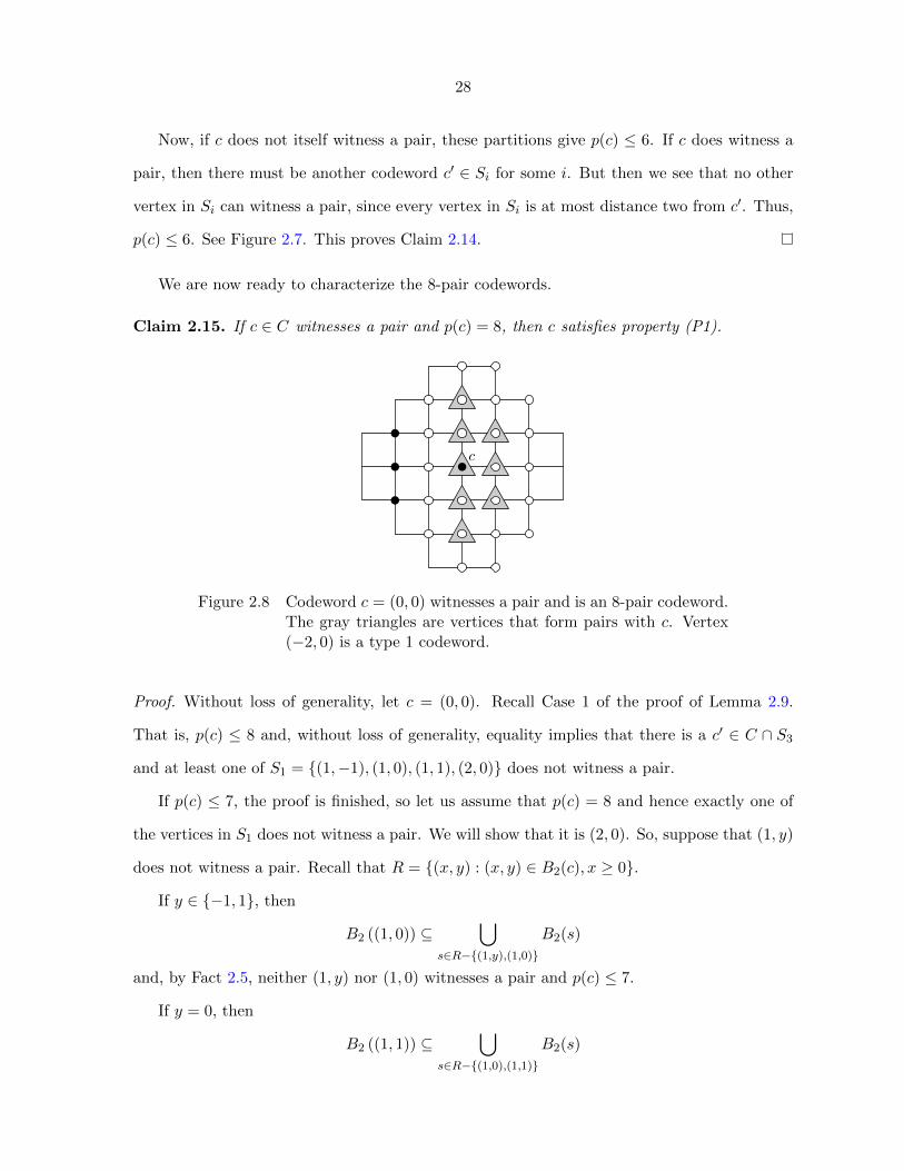
Claim 2.15. If c ∈ C witnesses a pair and p(c) = 8, then c satisfies property (P1).
c
Figure 2.8 Codeword c = (0, 0) witnesses a pair and is an 8-pair codeword.The gray triangles are vertices that form pairs with c. Vertex(−2, 0) is a type 1 codeword.
Proof. Without loss of generality, let c = (0, 0). Recall Case 1 of the proof of Lemma 2.9.
That is, p(c) ≤ 8 and, without loss of generality, equality implies that there is a c′ ∈ C ∩ S3
and at least one of S1 = {(1,−1), (1, 0), (1, 1), (2, 0)} does not witness a pair.
If p(c) ≤ 7, the proof is finished, so let us assume that p(c) = 8 and hence exactly one of
the vertices in S1 does not witness a pair. We will show that it is (2, 0). So, suppose that (1, y)
does not witness a pair. Recall that R = {(x, y) : (x, y) ∈ B2(c), x ≥ 0}.
If y ∈ {−1, 1}, then
B2 ((1, 0)) ⊆⋃
s∈R−{(1,y),(1,0)}
B2(s)
and, by Fact 2.5, neither (1, y) nor (1, 0) witnesses a pair and p(c) ≤ 7.
If y = 0, then
B2 ((1, 1)) ⊆⋃
s∈R−{(1,0),(1,1)}
B2(s)

29
and, by Fact 2.5, neither (1, 0) nor (1, 1) witnesses a pair and p(c) ≤ 7. It follows that each
vertex in R′ = R− {(2, 0)} must witness a pair containing c.
Each vertex which is distance 2 or less from 2 vertices in R′ cannot be a codeword. Thus,
(−2, 0) is the only vertex in B2(c) other than c which has not been marked as a non-codeword
and so (−2, 0) ∈ C. Since (0, 0) ∈ C, the vertex (−2, 1) is the only possibility for a second
codeword for (0, 1) and (−2,−1) is the only possibility for a second codeword for (0,−1). See
Figure 2.8.
Then (−2, 0) is a type 1 codeword and so it is in at most 4 pairs. Codewords (−2, 1) and
(−2,−1) are both adjacent to another codeword, so they are in at most 6 pairs. Hence, c
satisfies Property (P1). This proves Claim 2.15.
Claim 2.16. If c ∈ C does not witness a pair and p(c) = 8, then c satisfies either property
(P1) or property (P2).
Proof. Without loss of generality, let c = (0, 0). Recall Case 2 of the proof of Lemma 2.9.
That is, p(c) ≤ 8 and, without loss of generality, equality implies I2(c) = {c}. Furthermore,
one of the following two cases occurs:
(1) The eight witnesses are the vertices (±1, 0), (±2, 0), (0,±1) and (0,±2).
(2) The witnesses include {(1, 1), (−1, 1), (−1,−1), (1,−1)} as well as exactly one of each of
the following pairs: {(1, 0), (2, 0)}, {(0, 1), (0, 2)}, {(−1, 0), (−2, 0)} and
{(0,−1), (0,−2)}.
If case (1) occurs, then the eight witnesses are the vertices (±1, 0), (±2, 0), (0,±1) and
(0,±2). In this case, simply observe that B2((1, 0)) is a subset of the other seven witnesses.
This contradicts Fact 2.6 and so this case cannot occur.
So, we may assume that case (2) occurs. The vertex (2, 1) cannot be a codeword because
{(0, 0), (2, 1)} ⊆ B2((1, 1)), B2((1, 0)), B2((2, 0)) and so at most one of these three vertices
witness pairs, a contradiction to case (2). By symmetry, none of the following vertices are
codewords:
(2, 1), (1, 2), (−1, 2), (−2, 1), (−2,−1), (−1,−2), (1,−2), (2,−1).
30
c1c2
c3 c4
c s1
s2
s3
s4
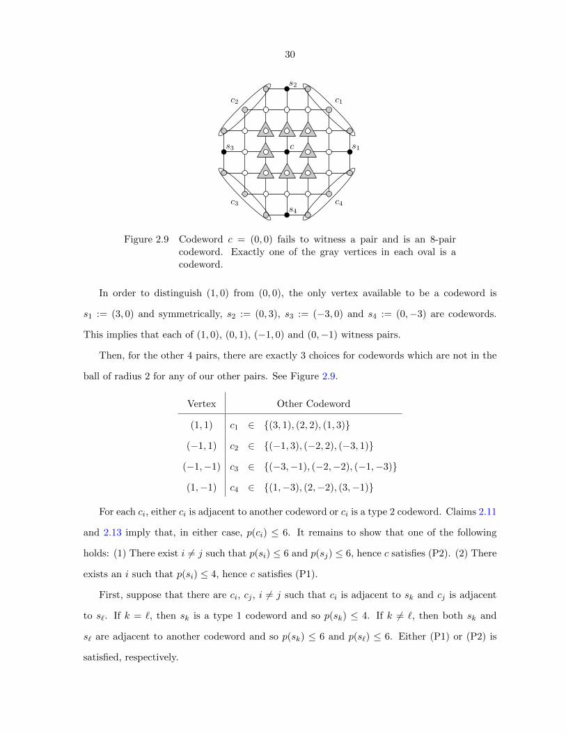
Figure 2.9 Codeword c = (0, 0) fails to witness a pair and is an 8-paircodeword. Exactly one of the gray vertices in each oval is acodeword.
In order to distinguish (1, 0) from (0, 0), the only vertex available to be a codeword is
s1 := (3, 0) and symmetrically, s2 := (0, 3), s3 := (−3, 0) and s4 := (0,−3) are codewords.
This implies that each of (1, 0), (0, 1), (−1, 0) and (0,−1) witness pairs.
Then, for the other 4 pairs, there are exactly 3 choices for codewords which are not in the
ball of radius 2 for any of our other pairs. See Figure 2.9.
Vertex Other Codeword
(1, 1) c1 ∈ {(3, 1), (2, 2), (1, 3)}
(−1, 1) c2 ∈ {(−1, 3), (−2, 2), (−3, 1)}
(−1,−1) c3 ∈ {(−3,−1), (−2,−2), (−1,−3)}
(1,−1) c4 ∈ {(1,−3), (2,−2), (3,−1)}
For each ci, either ci is adjacent to another codeword or ci is a type 2 codeword. Claims 2.11
and 2.13 imply that, in either case, p(ci) ≤ 6. It remains to show that one of the following
holds: (1) There exist i 6= j such that p(si) ≤ 6 and p(sj) ≤ 6, hence c satisfies (P2). (2) There
exists an i such that p(si) ≤ 4, hence c satisfies (P1).
First, suppose that there are ci, cj , i 6= j such that ci is adjacent to sk and cj is adjacent
to s`. If k = `, then sk is a type 1 codeword and so p(sk) ≤ 4. If k 6= `, then both sk and
s` are adjacent to another codeword and so p(sk) ≤ 6 and p(s`) ≤ 6. Either (P1) or (P2) is
satisfied, respectively.

31
If there is at most one ci such that ci is adjacent to sk for some k, then we have three
codewords of the form (±2,±2). Without loss of generality, assume that (2, 2), (2,−2), and
(−2, 2) are codewords. In this case, (3, 0) and (0, 3) are type 3 codewords and hence p((3, 0)) ≤
6 and p((0, 3)) ≤ 6. So again, (P2) is satisfied.
This proves Claim 2.16.
Finally, we can finish the proof of Lemma 2.10 by way of the discharging method. (For a
more extensive application of the discharging method on vertex identifying codes, see Cranston
and Yu [14].) Let Γ denote an auxiliary graph with vertex set C ∩ Qm for some m. There is
an edge between two vertices c and c′ if and only if I2(v) = {c, c′} for some v ∈ V (GS). For
each vertex v in our auxiliary graph Γ, we assign it an initial charge of d(v) − 7. Note that∑c∈C∩Qm
p(c)−7 =∑
v∈Γ degΓ(v)−7. We apply the following discharging rules if degΓ(v) = 8.
1. If v is adjacent to one vertex of degree at most 4 and two of degree at most 6 (condition
(P1)), then discharge 2/3 to a vertex of degree at most 4 and 1/6 to two vertices of
degree at most 6.
2. If v is adjacent to 6 vertices of degree at most 6 (condition (P2)), then discharge 1/6 to
6 neighbors of degree at most 6.
We have proven that one of the above cases is possible. Let e(v) be the charge of each
vertex after discharging takes place. We show that e(v) ≤ 0 for each vertex in Γ.
If degΓ(v) = 8, then our initial charge was 1. In either of the two cases, we are discharging
a total of 1 unit to its neighbors. Since no degree 8 vertex receives a charge from any other
vertex, we have e(v) = 0.
If d(v) = 7 then its initial charge is 0 and it neither gives nor receives a charge and so
e(v) = 0.
If 5 ≤ degΓ(v) ≤ 6, then its initial charge was at most −1. Since this vertex has at most 6
neighbors and can receive a charge of at most 1/6 from each of them, this gives e(v) ≤ 0.
If degΓ(v) ≤ 4, then its initial charge was at most −3. Since this vertex has at most 3
neighbors and can receive a charge of at most 2/3 from each of them, this gives e(v) ≤ −1/3 < 0.
32
Since no vertex can have degree more than 8, this covers all of the cases. Then we have
∑c∈C∩Qm
(p(c)− 7) =∑v∈Γ
(degΓ(v)− 7) =∑v∈Γ
e(v) ≤ 0.
Therefore, it follows that∑
c∈C∩Qmp(c) ≤
∑c∈C∩Qm
7 = 7|C ∩Qm|.
Proof of Theorem 2.3. Consider Qm and let C be an r-identifying code for GS and
C ∩Qm = {c1, c2, . . . , cK}. Recall inequality (2.1) from Theorem 2.7. In this case, b2 = 13 and
Lemma 2.10 shows that
Pm ≤1
2
∑c∈C∩Qm
p(c) ≤ 7
2|C ∩Qm|.
Substituting the above inequality into inequality (2.1) and rearranging gives
|C ∩Qm||Qm−r|
≥ 6
37.
Taking the limit as m→∞ gives the desired D(C) ≥ 6/37, completing the proof. �
2.5 Conclusions
The technique used for Lemma 2.7 is similar to the one in Cohen, Honkala, Lobstein and
Zemor [12]. Define
` = minc∈C|{v ∈ Br(c) : |Ir(v)| ≥ 3}|.
An anonymous referee points out that the computations in [12] can lead one to conclude that
D(C) ≥ 6
3br + 3− `. (2.2)
From our definitions
k = maxc∈C|{v ∈ Br(c) : |Ir(v)| = 2}|.
Since k + ` ≥ br − 1, one can use (2.2) to derive the result in Lemma 2.7.
As the referee also points out, k+` ≤ br, so the denominator could potentially be improved
by an additive factor of 1 if it were possible to show that k + ` = br.
Below is a table noting our improvements.

33
Hex Grid
r previous lower bounds new lower bounds upper bounds
2 2/11 ≈ 0.1818 [29] 1/5 = 0.2 4/19 ≈ 0.2105 [5]
3 2/17 ≈ 0.1176 [3] 3/25 = 0.12 1/6 ≈ 0.1667 [5]
Square Grid
2 3/20 = 0.15 [3] 6/37 ≈ 0.1622 5/29 ≈ 0.1724 [26]
This technique works quite well for small values of r, but we note that br = |Br(v)| grows
quadratically in r, so the denominator in Lemma 2.7 would grow quadratically. But the known
the lower bounds for r-identifying codes is proportional to 1/r in all of the well-studied grids
(square, hexagonal, triangular and king). Therefore, our technique is less effective as r grows.
Acknowledgements
We would like to thank an anonymous referee for making helpful suggestions and directing
us to the paper [12].

34
CHAPTER 3. IMPROVED BOUNDS FOR r-IDENTIFYING CODES
OF THE HEX GRID
Based on a paper published in SIAM Journal on Discrete Mathematics
Brendon Stanton
Abstract
For any positive integer r, an r-identifying code on a graph G is a set C ⊂ V (G) such
that for every vertex in V (G), the intersection of the radius-r closed neighborhood with C is
nonempty and pairwise distinct. For a finite graph, the density of a code is |C|/|V (G)|, which
naturally extends to a definition of density in certain infinite graphs which are locally finite.
We find a code of density less than 5/(6r), which is sparser than the prior best construction
which has density approximately 8/(9r).
3.1 Introduction
Given a connected, undirected graph G = (V,E), define Br(v), called the ball of radius r
centered at v, to be
Br(v) = {u ∈ V (G) : d(u, v) ≤ r},
where d(u, v) is the distance between u and v in G.
We call any C ⊂ V (G) a code. We say that C is r-identifying if C has the following
properties:
1. Br(v) ∩ C 6= ∅ for all v ∈ V (G) and
2. Br(u) ∩ C 6= Br(v) ∩ C for all distinct u, v ∈ V (G).

35
The elements of C are called codewords. We define Ir(v) = Ir(v, C) = Br(v) ∩ C. We call
Ir(v) the identifying set of v with respect to C. If Ir(u) 6= Ir(v) for some u 6= v, we say u and
v are distinguishable. Otherwise, we say they are indistinguishable.
Vertex identifying codes were introduced in [29] as a way to help with fault diagnosis in
multiprocessor computer systems. Codes have been studied in many graphs. Of particular
interest are codes in the infinite triangular, square, and hexagonal lattices as well as the square
lattice with diagonals (king grid). We can define each of these graphs so that they have vertex
set Z × Z. Let Qm denote the set of vertices (x, y) ⊂ Z × Z with |x| ≤ m and |y| ≤ m. The
density of a code C defined in [5] is
D(C) = lim supm→∞
|C ∩Qm||Qm|
.
When examining a particular graph, we are interested in finding the minimum density of
an r-identifying code. The exact minimum density of an r-identifying code for the king grid
was found in [4]. General constructions of r-identifying codes for the square and triangular
lattices are given in [26] and [3].
For this paper, we focus on the hexagonal grid. It was shown in [3] that
2
5r− o(1/r) ≤ D(GH , r) ≤
8
9r+ o(1/r),
where D(GH , r) represents the minimum density of an r-identifying code in the hexagonal grid.
The main theorem of this paper is Theorem 3.1:
Theorem 3.1. There exists an r-identifying code of density
5r + 3
6r(r + 1)if r is even;
5r2 + 10r − 3
(6r − 2)(r + 1)2if r is odd.
The proof of Theorem 3.1 can be found in Section 3.4. Section 3.2 provides a brief
description of a code with the aforementioned density and gives a few basic definitions needed
to describe the code. Section 3.3 provides a few technical lemmas needed for the proof of
Theorem 3.1 and the proofs of these lemmas can be found in Section 3.5.

36
Figure 3.1 The code C = C ′∪C ′′ for r = 6. Black vertices are code words.White vertices are vertices in Ln(r+1) which are not in C.
3.2 Construction and Definitions
For this construction we will use the brick wall representation of the hex grid. To describe
this representation, we need to briefly consider the square grid GS . The square grid has vertex
set V (GS) = Z× Z and
E(GS) = {{u = (i, j), v} : u− v ∈ {(0,±1), (±1, 0)}}.
Let GH represent the hex grid. Then V (GH) = Z× Z and
E(GH) = {{u = (i, j), v} : u− v ∈ {(0, (−1)i+j+1), (±1, 0)}}.
In other words, if x+y is even, then (x, y) is adjacent to (x, y+1), (x−1, y), and (x+1, y).
If x+ y is odd, then (x, y) is adjacent to (x, y− 1), (x− 1, y), and (x+ 1, y). However, the first
representation shows clearly that the hex grid is a subgraph of the square grid.
For any integer k, we also define a horizontal line Lk = {(x, k) : x ∈ Z}.
Note that if u, v ∈ V (GS), then the distance between them (in the square grid) is ‖u− v‖1.
From this point forward, let d(u, v) represent the distance between two vertices in the hex
grid. If u ∈ V (GH) and U, V ⊂ (GH), we define d(u, V ) = min{d(u, v) : v ∈ V } and
d(U, V ) = min{d(u, V ) : u ∈ U}.

37
Figure 3.2 The code C = C ′∪C ′′ for r = 7. Black vertices are code words.White vertices are vertices in Ln(r+1) which are not in C.
Let δ = 0 if k is even and δ = 1 otherwise. Define
L′k =
Lk ∩ {(x, k) : x 6≡ 1, 3, 5, . . . , r − 1 mod 3r} if r is even;
Lk ∩ {(x, k) : x 6≡ 1, 3, 5, . . . , r − 1 mod 3r − 1} if r is odd
and
L′′k =
Lk ∩ {(x, k) : x ≡ δ mod r} if r is even;
Lk ∩ {(x, k) : x ≡ 0 mod r + 1} if r is odd.
Finally, let
C ′ =
∞⋃n=−∞
L′n(r+1) and C ′′ =
∞⋃n=−∞
L′′b(r+1)/2c+2n(r+1).
Let C = C ′ ∪ C ′′. We will show in Section 3.4 that C is a valid r-identifying code of the
density described in Theorem 3.1. Partial pictures of the code are shown for r = 6 in Figure
3.1 and r = 7 in Figure 3.2.
3.3 Distance Claims
We present a list of lemmas on the distances of vertices in the hex grid. These lemmas will
be used in the proof of our construction. The proofs of these lemmas can be found in Section
3.5.

38
Lemma 3.2. For u, v ∈ V (GH), d(u, v) ≥ ‖u− v‖1.
Proof. Note that Lemma 3.2 simply says that the distance between any two vertices in our
graph is no less than the their distance in the square grid. Since GH is a subgraph of GS , any
path between u and v in GH is also a path in GS and so the lemma follows.
Lemma 3.3. (Taxicab Lemma) For u = (x, y), v = (x′y′) ∈ V (GH), if |x − x′| ≥ |y − y′|,
then d(u, v) = ‖u− v‖1.
This fact is used so frequently that we call it the Taxicab Lemma. It states that if the
horizontal distance between two vertices is no less than the vertical distance, then the distance
between those two vertices is exactly the same as it would be in the square grid.
The proof of the Taxicab Lemma and the remainder of these lemmas can be found in
Section 3.5.
Lemmas 3.4 and 3.5 say that the distance between a point (k, a) and a line Lb is either
2|a − b| or 2|a − b| − 1 depending on various factors. It also follows from these lemmas that
d(La, Lb) = 2|a− b| − 1 if a 6= b.
Lemma 3.4. Let a < b; then
d((k, a), Lb) =
2(b− a)− 1, if a+ k is even;
2(b− a), if a+ k is odd.
Lemma 3.5. Let a > b; then
d((k, a), Lb) =
2(a− b) if a+ k is even;
2(a− b)− 1 if a+ k is odd.
The next three lemmas all basically have the same idea. If we are looking at a point (x, y)
and a horizontal line Lk such that (x, y) is within some given distance d, we can find a sequence
S of points on this line such that each point is at most distance d from (x, y) and the distance
between each point in S and its closest neighbor in S is exactly 2.

39
Lemma 3.6. Let k be a positive integer. There exist paths of length 2k from (x, y) to v for
each v in
{(x− k + 2j, y ± k) : j = 0, 1, . . . , k}.
Lemma 3.7. Let k be a positive integer and let x + y be even. There exist paths of length
2k + 1 from (x, y) to v for each v in
{(x− k + 2j, y + k + 1) : j = 0, 1, . . . , k} ∪ {(x− k − 1 + 2j, y − k) : j = 0, 1, . . . , k + 1}.
Lemma 3.8. Let k be a positive integer and let x+y be odd. There exist paths of length 2k+1
from (x, y) to v for each v in
{(x− k + 2j, y − k − 1) : j = 0, 1, . . . , k} ∪ {(x− k − 1 + 2j, y + k) : j = 0, 1, . . . , k + 1}.
In the final lemma, we are simply stating that if we are given a point (x, y) and a line Lk
such that d((x, y), Lk) < r, we can find a path of vertices on that line which are all distance
at most r from (x, y).
Lemma 3.9. Let (x, y) be a vertex and Lk be a line. If d((x, y), Lk) < r, then
{(x− (r − |y − k|) + j, k) : j = 0, 1, . . . , 2(r − |y − k|)} ⊂ Br((x, y)).
3.4 Proof of Main Theorem
Here, we wish to show that the set described in Section 3.2 is indeed a valid r-identifying
code.
Proof of Theorem 3.1.
Let C = C ′ ∪ C ′′ be the code described in Section 3.2. Let d(C) be the density of C in
GH , d(C ′) be the density of C ′ in GH , and d(C ′′) be the density of C ′′ in GH . Since C ′ and
C ′′ are disjoint, we see that

40
d(C) = lim supm→∞
|C ∩Gm||Gm|
= lim supm→∞
|(C ′ ∪ C ′′) ∩Gm||Gm|
= lim supm→∞
|C ′ ∩Gm||Gm|
+ lim supm→∞
|C ′′ ∩Gm||Gm|
= d(C ′) + d(C ′′).
It is easy to see that both C ′ and C ′′ are periodic tilings of the plane (and hence C is also
periodic). The density of periodic tilings was discussed By Charon, Hudry, and Lobstein [5]
and it is shown that the density of a periodic tiling on the hex grid is
D(C) =# of codewords in tile
size of tile.
For r even, we may consider the density of C ′ on the tile [0, 3r− 1]× [0, r]. The size of this
tile is 3r(r + 1). On this tile, the only members of C ′ fall on the horizontal line L0, of which
there are 2r + r/2.
For r odd, we may consider the density of C ′ on the tile [0, 3r − 2] × [0, r]. The size of
this tile is (3r − 1)(r + 1). On this tile, the only members of C ′ fall on L0, of which there are
2r + (r − 1)/2. Thus
d(C ′) =
5
6(r+1) if r is even;
5r−1(6r−2)(r+1) if r is odd.
For C ′′, we need to consider the tiling on [0, r−1]×[0, 2r+1] if r is even and [0, r]×[0, 2r+1]
if r is odd. In either case, the tile contains only a single member of C ′′. Hence,
d(C ′′) =
1
2r(r+1) if r is even;
12(r+1)2
if r is odd.
Adding these two densities together gives us the numbers described in the theorem.
It remains to show that C is a valid code. We will say that a vertex v is nearby L′k if
Ir(v) ∩ L′k 6= ∅. An outline of the proof is as follows:

41
1. Each vertex v ∈ V (GH) is nearby L′n(r+1) for exactly one value of n (and hence, Ir(v) 6=
∅).
2. Since each vertex is nearby L′n(r+1) for exactly one value of n, we only need to distinguish
between vertices which are nearby the same horizontal line.
3. The vertices in C ′′ distinguish between vertices that fall above the horizontal line and
those that fall below the line.
4. We then show that L′n(r+1) can distinguish between any two vertices which fall on the
same side of the horizontal line (or in the line).
Part (1): We want to show that each vertex is nearby Ln(r+1) for exactly one value of n.
From Lemma 3.4, it immediately follows that d(Ln(r+1), L(n+1)(r+1)) = 2r + 1. So by the
triangle inequality, no vertex can be within a distance r of both of these lines. Thus, no vertex
can be nearby more than one horizontal line of the form Ln(r+1).
Lemma 3.10. Let u, v ∈ Ln(r+1). Then
1. If u ∼ v then at least one of u and v is in C ′.
2. If r ≤ d(u, v) ≤ 2r + 1, then at least one of u and v is in C ′.
Furthermore, note that for any x at least one of the following vertices is in C:
{(x+ 2k, n(r + 1)) : k = 0, 1, . . . , d(r + 1)/2e}.
The proof of this lemma is in Section 3.5.
From this point forward, let v = (i, j) with n(r + 1) ≤ j < (n+ 1)(r + 1).
First, suppose that r is even. Then for j ≤ r/2+n(r+1) we have d((i, j), (i−r/2, j−r/2)) =
r by the Taxicab Lemma. Since j−r/2 ≤ n(r+1), there is u ∈ Ln(r+1) such that d((i, j), u) ≤ r.
If d((i, j), u) < r, then u and u+ (1, 0) are both within distance r of (i, j) and by Lemma 3.10
one of them is in C ′. If d((i, j), Ln(r+1)) = r, then by Lemma 3.6 (i, j) is within distance r of
one of the vertices in the set {(i− r/2 + 2k : k = 0, 1, . . . , r/2} and again by Lemma 3.10 one
42
of them must be in C ′. By a symmetric argument, we can show that if j > r/2, then there is
a u ∈ C ′ ∩ L(n+1)(r+1) such that d((i, j), u) ≤ r.
If r is odd, and j 6= (r + 1)/2, then we can use the same argument to show there is a
codeword in C ′ ∩ L(n+1)(r+1) or C ′ ∩ L(n+1)(r+1) within distance r of (i, j). If j = (r + 1)/2,
then we refer to Lemmas 3.7, 3.8, and 3.10 to find an appropriate codeword. Since no vertex
can be nearby more than one horizontal line of the form Ln(r+1), this shows that each vertex
is nearby exactly one horizontal line of this form.
So we have shown that v is nearby exactly one horizontal line of the form L′n(r+1), but this
also shows that Ir(v) 6= ∅ for any v ∈ V (GH).
Part (2): We now turn our attention to showing that Ir(u) 6= Ir(v) for any u 6= v. We
first note that if u is nearby L′n(r+1), v is nearby L′m(r+1), and m 6= n, then there is some c in
Ir(v)∩L′m(r+1) but c 6∈ Ir(u) since u is not nearby L′m(r+1). Thus, u and v are distinguishable.
Hence it suffices to consider only the case that n = m.
Part (3): We consider the case that u and v fall on opposite sides of Ln(r+1). Suppose
that u = (i, j), where j > n(r + 1) and v = (i′, j′), where j′ < n(r + 1). We see that if
n = 2k, then n(r + 1) < b(r + 1)/2c + 2k(r + 1) < (n + 1)(r + 1) and if n = 2k + 1, then
(n− 1)(r + 1) < b(r + 1)/2c+ 2k(r + 1) < n(r + 1). In the first case, we see that
d((i′, j′), Lb(r+1)/2c+2k(r+1)) ≥ d(L2k(r+1)−1, Lb(r+1)/2c+2k(r+1))
= 2b(r + 1)/2c+ 1
≥ r + 1
and likewise in the second case we have that d((i, j), Lb(r+1)/2c+2k(r+1)) ≥ r+1 and so it follows
that at most one of (i, j) and (i′, j′) is within distance r of a codeword in C ′′.
If r is odd, then b(r+ 1)/2c = (r+ 1)/2 and |j− (r+ 1)/2 + 2k(r+ 1)| ≤ (r− 1)/2. Hence,
we see that d((i, j), L(r+1)/2+2k(r+1)) ≤ r − 1. From Lemma 3.9, it follows that
{(m, (r + 1)/2 + n(r + 1)) : (r − 1)/2 ≤ m ≤ (3r − 1)/2} ⊂ Br((i, j)).
We note that the cardinality of this set is at least r+ 1 and so in the case that n is even we see
that at least one of these must be in C ′′. A symmetric argument applies if n is odd, showing

43
that (i′, j′) is within distance r of a codeword in C ′′.
If r is even, we apply a similar argument to show that (i, j) is within distance r − 1 of r
vertices in Ln(r+1)+b(r+1)/2c and (i′, j′) is within distance r of r−1 vertices of Ln(r+1)−d(r+1)/2e.
If n is even, then clearly (i, j) is within distance r of some codeword in C ′′. However, if n is
odd, we have only shown that
{(m, d(r + 1)e/2 + n(r + 1)) : r/2− 2 ≤ m ≤ 3r/2− 1} ⊂ Br−1((i, j)).
Consider the set
{(m, b(r + 1)c/2 + n(r + 1)) : r/2− 2 ≤ m ≤ 3r/2− 1}.
This set has r vertices and so one of them must be a codeword. Furthermore, by the way
we constructed C ′′, the sum of the coordinates of codeword are even and so there is an edge
connecting it to a vertex in
{(m, d(r + 1)e/2 + n(r + 1)) : r/2− 2 ≤ m ≤ 3r/2− 1}
and so it is within radius r of (i′, j′). In either case, we have exactly one of u and v is within
distance r of a codeword in C ′′.
Part (4): Now we have shown that two vertices are distinguishable if they are nearby two
different lines in C ′ or if they fall on opposite sides of a line Ln(r+1) for some n. To finish our
proof, we need to show that we can distinguish between u = (i, j) and v = (i′, j′) if u and v
are nearby the same line L′n(r+1) and u and v fall on the same side of that line. Without loss
of generality, assume that j, j′ ≥ n(r + 1).
Case 1: u, v ∈ Ln(r+1).
Without loss of generality, we can write u = (x, n(r+1)) and v = (x+k, n(r+1)) for k > 0.
If k > 1, then (x − r, n(r + 1)) and (x − r + 1, n(r + 1)) are both within distance r of u but
not of v and one of them must be a codeword by Lemma 3.10. If k = 1, then (x− r, n(r + 1))
is within distance r of u but not v and (x+ r+ 1, n(r+ 1)) is within distance r of v but not u.
Since d((x − r, n(r + 1)), (x + r + 1, n(r + 1))) = 2r + 1, Lemma 3.10 states that at least one
of them must be a codeword.

44
Case 2: u ∈ Ln(r+1), v 6∈ Ln(r+1).
Without loss of generality, assume that i ≤ i′. We have u = (i, n(r + 1)). If i = i′, then
v = (i, n(r+ 1) + k) for some k > 0. Consider the vertices (i− r, n(r+ 1)) and (i+ r, n(r+ 1)).
These are each distance r from u and they are distance 2r from each other, so by Lemma
3.10 at least one of them is a codeword. However, by Lemma 3.2, these are distance at least
r + k > r from v and so Ir(u) 6= Ir(v).
If i < i′, then we can write v = (i + j, n(r + 1) + k) for j, k > 0. Consider the vertices
x1 = (i − r, n(r + 1)) and x2 = (i − r + 1, n(r + 1)). By the Taxicab Lemma, d(u, x1) = r
and d(u, x2) = r − 1. Further, since they are adjacent vertices in Ln(r+1), one of them is in
C ′ by Lemma 3.10. However, by Lemma 3.2 we have d(v, x1) ≥ r + j + k > r and d(v, x2) ≥
r − 1 + j + k > r. Hence, neither of them is in Ir(v) and so Ir(u) 6= Ir(v).
Case 3: u, v 6∈ Ln(r+1).
Assume without loss of generality that n = 0 and so 1 ≤ j, j′ ≤ dr/2e.
Subcase 3.1: j < j′, i = i′.
From Lemma 3.5 it immediately follows that d((i, j), L0) < d((i′, j′), L0) ≤ r. By the
Taxicab Lemma, we have d((i−(r−j), 0), (i, j)) = d((i+(r−j), 0), (i, j)) = r. Further note that
d((i−(r−j), (i+(r−j), 0)) = 2(r−j) and since 1 ≤ j < dr/2e we have r+1 ≤ 2(r−j) ≤ 2r−2
and so at least one of these two vertices is a codeword by Lemma 3.10. By the Taxicab Lemma,
neither of these two vertices is in Br((i′, j′)).
Subcase 3.2: j < j′, i 6= i′.
Without loss of generality, we may assume that i < i′. Then, we wish to consider the
vertices (i− (r− j), 0) and (i− (r− j) + 1, 0). We see that d((i, j), (i− (r− j) + 1, 0)) = r− 1
and so by the Taxicab Lemma, neither of these vertices is in Br((i′, j′)). But since these
vertices are adjacent and both in L0 at least one of them is a codeword by Lemma 3.10 and
so that one is in Ir((i, j)) but not in Ir((i′, j′)).
Subcase 3.3: j = j′, d(u, L0) < r or d(v, L0) < r.
Without loss of generality, assume that d((i, j), L0) < r and that i < i′. Then v = (i+k, j)
for some k > 0.

45
First suppose that k > 1. Then, we wish to consider the vertices (i − (r − j), 0) and
(i − (r − j) + 1, 0). We see that d((i, j), (i − (r − j) + 1, 0)) = r − 1 and so by the Taxicab
Lemma, neither of these vertices is in Br((i′, j′)). But since these vertices are adjacent and
both in L0, by Lemma 3.10 at least one of them is a codeword and so that one is in Ir((i, j))
but not in Ir(i′, j′)).
If k = 1, consider the vertices x1 = (i− (r− j), 0) and x2 = (i+ 1 + (r− j), 0). We see that
d(x1, u) = r,
d(x1, v) = r + 1,
d(x2, u) = r + 1,
d(x2, v) = r
all by the taxicab lemma. Furthermore, d(x1, x2) = 2(r−j)+1 and so r+1 ≤ d(x1, x2) ≤ 2r+1
as in the above case and so one of them is a code word by Lemma 3.10. Hence Ir(u) 6= Ir(v).
Subcase 3.4: j = j′, d(u, L0) = d(v, L0) = r.
Without loss of generality, suppose i′ < i. We wish to consider the vertices in the two sets
U = {(i− (r − j) + 2k, 0) : k = 0, 1, 2, . . . , r − j}
and
V = {(i′ − (r − j) + 2k, 0) : k = 0, 1, 2, . . . , r − j}.
Note that
|U | = |V | =
r/2 + 1 if r is even,
(r + 1)/2 if r is odd.
From Lemmas 3.6, 3.7, and 3.8 we have U ⊂ Br(u) and V ⊂ Br(v). Each of U and V
contain a codeword by Lemma 3.10. Hence, if U ∩ V = ∅ then u and v are distinguishable.
If U ∩ V 6= ∅ then the leftmost vertex in U is also in V . We further note that the leftmost
vertex in U is not the leftmost vertex in V or else U = V and u = v. Thus, we must have
i′ − (r − j) + 2 ≤ i ≤ i′ + (r − j) and so 2 ≤ i − i′ ≤ 2(r − j). Let x1 = (i + (r − j), 0) and
let x2 = (i′ − (r − j), 0). By definition x1 ∈ U and x2 ∈ V . By the Taxicab Lemma we have
d(x1, v) = |i+r−j−i′|+|j| = r+i−i′ > r and likewise d(x2, u) > r so x1 6∈ Ir(v) and x2 6∈ Ir(u).

46
Also we have d(x1, x2) = 2(r− j) + i− i′ which gives 2(r− j) + 2 ≤ d(x1, x2) ≤ 4(r− j). Since
d(u, L0) = r we must have r− j = r/2 if r is even and r− j = (r− 1)/2 if r is odd by Lemmas
3.4 and 3.5. In either case this gives r + 2 ≤ d(x1, x2) ≤ 2r. By Lemma 3.10, one of x1 and
x2 is a codeword and so u and v are distinguishable.
This completes the proof of Theorem 3.1. �
3.5 Proof of Lemmas
We now complete the proof by going back and finishing off the proofs of the lemmas that
were presented in Section 3.3.
Proof of Lemma 3.3. (Taxicab Lemma) By Lemma 3.2, it suffices to show there exists
a path of length ‖u − v‖ between u and v. Since |x − x′| ≥ |y − y′|, either u = v or x 6= x′.
If u = v, then the lemma is trivial, so assume without loss of generality that x < x′. We will
first assume that y ≤ y′.
We note that no matter what the parity of i + j, there is always a path of length 2 from
(i, j) to (i + 1, j + 1). Then for 1 ≤ i ≤ |y − y′|, define Pi to be the path of length 2 from
(x+ i− 1, y + i− 1) to (x+ i, y + i). Then⋃|y−y′|
i=1 Pi is a path of length 2(y′ − y) from (x, y)
to (x+ y′− y, y′). Since (i, j) ∼ (i+ 1, j) for all i, j, there is a path P ′ of length x′− x+ y− y′
(Note: this number is nonnegative since x′ − x ≥ y′ − y.) from (x + y′ − y, y′) to (x′, y′) by
simply moving from (i, y′) to (i + 1, y′) for x + y′ − y ≤ i < x′. Then, we calculate the total
length of
P ′ ∪|y−y′|⋃i=1
Pi
to be |x′ − x|+ |y′ − y|. By Lemma 3.2, it follows that d(u, v) = |x− x′|+ |y − y′| = ‖u− v‖1.
If y > y′, then a symmetric argument follows by simply following a downward diagonal
followed by a straight path to the right. �
Proof of Lemma 3.4. We proceed by induction on b− a.
The base case is trivial since if a + k is even, then (k, a) ∼ (k, a + 1) = (k, b). If a + k is
odd, then there is no edge directly to Lb and so any path from (k, a) to Lb has length at least

47
2. This is attainable by the path from (k, a) to (k + 1, a) to (k + 1, b).
The inductive step follows similarly. Let a + k be even. Then there is an edge between
(k, a) and (k, a+ 1). Since k+ a+ 1 is odd, the shortest path from (k, a+ 1) to Lb has length
2(b − a − 1) and so the union of that path with the edge {(k, a), (k, a + 1)} gives a path of
length 2(b− a)− 1. Likewise, if k+ a is odd, then we take the path from (k, a) to (k+ a, a) to
(k+ 1, a+ 1) in union with a path from (k+ 1, a+ 1) to Lb gives us a path of length 2(b− a).
Further, any path from La to Lb must contain at least one point in La+1. So if we take a path
of length ` from (k, a) to (j, a + 1) (note that j + a + 1 must be odd), then we get a path
of length ` + 2(b − a − 1). From the base case, we have chosen our paths from La to La+1
optimally and so this path is minimal. �
Proof of Lemma 3.5. The proof is symmetric to the previous proof. �
Proof of Lemma 3.6. The proof is by induction on k. If k = 1, then as noted before, there
is always a path of length 2 from (x, y) to (x± 1, y ± 1).
For k > 1, there is a path of length 2 from (x, y) to (x− 1, y+ 1) and to (x+ 1, y+ 1). By
the inductive hypothesis, there is a path of length 2(k− 1) from (x− 1, y+ 1) to each vertex in
S = {(x− k + 2j, y + k) : j = 0, 1, . . . , k − 1}
and a path of length 2(k−1) from (x+ 1, y+ 1) to (x+k, y+k). Taking the union of the path
of length 2 from (x, y) to (x− 1, y + 1) and the path of length 2(k − 1) from (x− 1, y + 1) to
each vertex in S gives us a path of length 2k to each vertex in
{(x− k + 2j, y + k) : j = 0, 1, . . . , k − 1}.
Then, taking the path of length 2 from (x, y) to (x+ 1, y + 1) and the path of length 2(k − 1)
from (x+ 1, y + 1) to (x+ k, y + k) gives us a path of length 2k from (x, y) to each vertex in
{(x− k + 2j, y + k) : j = 0, 1, . . . , k}.
By a symmetric argument, we can find paths of length 2k from (x, y) to each vertex in
{(x− k + 2j, y − k) : j = 0, 1, . . . , k}.
48
�
Proof of Lemma 3.7. Since x + y is even, (x, y) ∼ (x, y + 1). By Lemma 3.6, there are
paths of length 2k from (x, y + 1) to each vertex in {(x − k + 2j, y + k + 1) : j = 0, 1, . . . , k}
and hence there are paths of length 2k + 1 from (x, y) to each vertex in that set.
Since (x, y) ∼ (x − 1, y), by Lemma 3.6, there are paths of length 2k from (x − 1, y) to
each vertex in {(x − k − 1 + 2j, y − k) : j = 0, 1, . . . , k}. Similarly, since (x, y) ∼ (x + 1, y)
there is a path of length 2k from (x+ 1, y) to (x+ k+ 1, y− k) and so there is a path of length
2k + 1 from (x, y) to each vertex in {(x− k − 1 + 2j, y − k) : j = 0, 1, . . . , k + 1}. �
Proof of Lemma 3.8. Since x + y is odd, (x, y) ∼ (x, y − 1). By Lemma 3.6, there are
paths of length 2k from (x, y − 1) to each vertex in {(x − k + 2j, y − k − 1) : j = 0, 1, . . . , k}
and hence there are paths of length 2k + 1 from (x, y) to each vertex in that set.
Since (x, y) ∼ (x − 1, y), by Lemma 3.6, there are paths of length 2k from (x − 1, y) to
each vertex in {(x − k − 1 + 2j, y + k) : j = 0, 1, . . . , k}. Similarly, since (x, y) ∼ (x + 1, y)
there is a path of length 2k from (x+ 1, y) to (x+ k+ 1, y+ k) and so there is a path of length
2k + 1 from (x, y) to each vertex in {(x− k − 1 + 2j, y + k) : j = 0, 1, . . . , k + 1}. �
Proof of Lemma 3.9. Without loss of generality, assume that y ≥ k. If y = k, the Lemma is
trivial, so let ` > 0 be the length of the shortest path between (x, y) and Lk. By assumption,
` ≤ r − 1.
First assume that ` is even. By Lemma 3.6, there is a path of length ` from (x, y) to
each vertex in S = {((x − `/2 + 2j, k) : j = 0, 1, . . . , `/2}. Note that the vertices in the set
S′ = {((x − `/2 + 2j − 1, k) : j = 0, 1, . . . , `/2 + 1} all fall within distance 1 of a vertex in S
and so S ∪ S′ = {((x− `/2− 1 + j, k) : j = 0, 1, . . . , `+ 2} ⊂ Br((x, y)).
Now note that d((x, y), (x− `/2, k)) = `, so if x− (r− |y− k|) ≤ x0 ≤ x− `/2 for some x0,
then
d((x0, k), (x, y)) ≤ d((x0, k), (x− `/2, k)) + d((x− `/2, k), (x, y))
≤ (r − |y − k| − `/2) + `.

49
Since |y− k| = `/2 this gives d((x0, k), (x, y)) ≤ r. Likewise, if x+ `/2 ≤ x0 ≤ x+ (r− |y− k|)
for some x0, then d((x0, k), (x, y)) ≤ r. Hence, d((x0, k), (x, y)) ≤ r for all x− (r − |y − k|) ≤
x0 ≤ x+ (r − |y − k|) and so the Lemma follows.
If ` is odd, the Lemma follows by using either Lemma 3.7 or Lemma 3.8 and applying a
similar argument.
�
Proof of Lemma 3.10. This first part of this lemma is immediate from the definition of C ′
since the only vertices in Ln(r+1) which are not in L′n(r+1) are separated by distance 2. To see
the second part, let ` = 3r if r is even and ` = 3r− 1 if r is odd. Write L′n(r+1) = S1 ∪S2 ∪S3,
where
S1 = L′n(r+1) ∩ {(x, y), x ≡ 1, . . . , r − 1 mod `},
S2 = L′n(r+1) ∩ {(x, y), x ≡ r, r + 1, . . . , 2r − 1 mod `},
S3 = L′n(r+1) ∩ {(x, y), x ≡ 2r, 2r + 1, . . . , ` mod `}.
Note that each vertex in S2 ∪ S3 is in C ′ and so if u, v ∈ Ln(r+1) are both not in C ′, they are
both in S1. However, it is clear that for two vertices in S1, that their distance is either strictly
less than r or at least than 2r + 1.
Finally, for the last part of the lemma, we use the same partition of Ln(r+1) so that all
noncodewords fall in S1. However, the distance between (x, n(r + 1)) and (x + 2d(r + 1)/2e)
is at least r + 1 so one of those two vertices cannot fall in S1 and so it is a codeword. �
3.6 Conclusion
In an upcoming paper, we also provide improved lower bounds for D(GH , r) when r = 2
or r = 3 [34]. Below are a couple tables noting our improvements. This includes the results
not only from our paper, but also from the aforementioned paper.

50
Hex Grid
r previous lower bounds new lower bounds upper bounds
2 2/11 ≈ 0.1818 [29] 1/5 = 0.2 [34] 4/19 ≈ 0.2105 [5]
3 2/17 ≈ 0.1176 [3] 3/25 = 0.12 1/6 ≈ 0.1667 [5]
Square Grid
2 3/20 = 0.15 [3] 6/37 ≈ 0.1622 [34] 5/29 ≈ 0.1724 [26]
Hex Grid
r lower bounds new upper bounds previous upper bounds
15 2/77 ≈ 0.0260 [3] 1227/22528 ≈ 0.0523 1/18 ≈ 0.0556 [5]
16 2/83 ≈ 0.0241 [3] 83/1632 ≈ 0.0509 1/18 ≈ 0.0556 [5]
17 2/87 ≈ 0.0230 [3] 1/22 ≈ 0.0455 [5]
18 2/93 ≈ 0.0215 [3] 31/684 ≈ 0.0453 1/22 ≈ 0.0455 [5]
19 2/97 ≈ 0.0206 [3] 387/8960 ≈ 0.0432 1/22 ≈ 0.0455 [5]
20 2/103 ≈ 0.0194 [3] 103/2520 ≈ 0.0409 1/22 ≈ 0.0455 [5]
21 2/107 ≈ 0.0187 [3] 1/26 ≈ 0.0385 [5]
For even r ≥ 22, we have improved the bound from approximately 8/(9r) [3] to (5r +
3)/(6r(r+ 1)) and for odd r ≥ 23 we have improved the bound from approximately 8/(9r) [3]
to (5r2 + 7r − 3)/((6r − 2)(r + 1)2).
Constructions for 2 ≤ r ≤ 30 given in [5] were previously best known. However, the best
general constructions were given in [3].
Acknowledgement
The author would like to thank anonymous referees whose comments improved the manuscript.

51
CHAPTER 4. VERTEX IDENTIFYING CODES FOR THE
n-DIMENSIONAL LATTICE
Based on a paper submitted to Discrete Mathematics
Brendon Stanton
Abstract
An r-identifying code on a graph G is a set C ⊂ V (G) such that for every vertex in V (G),
the intersection of the radius-r closed neighborhood with C is nonempty and different. If
n = 2k − 1 for some integer k, it is easy to show that an optimal 1-identifying code can be
constructed for the n-dimensional lattice through a construction using a Hamming code. Here,
we show how to construct sparse codes in the case that n 6= 2k−1 by giving two different types
of constructions. In addition, we provide a better bound for the 4-dimensional case through a
connection with the king grid. We also prove a monotonicity theorem for r-identifying codes
on the n-dimensional lattice and show that for fixed n, the minimum density of an r-identifying
code is Θ(1/rn−1).
4.1 Introduction
Vertex identifying codes were introduced by Karpovsky, Chakrabarty, and Levitin in [29]
as a way to help with fault diagnosis in multiprocessor computer systems. That paper also
addresses the issue of finding codes on a wide variety of graphs including the square, hexagonal
and triangular lattices and the n-dimensional hypercube. In addition, it briefly explores the
idea of codes on the n-dimensional hypercube with pn vertices. Taking the limit as p→∞ we
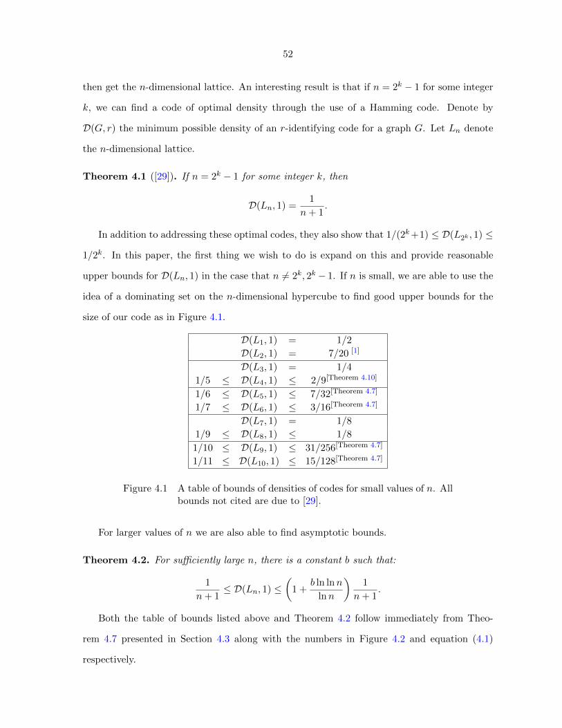
52
then get the n-dimensional lattice. An interesting result is that if n = 2k − 1 for some integer
k, we can find a code of optimal density through the use of a Hamming code. Denote by
D(G, r) the minimum possible density of an r-identifying code for a graph G. Let Ln denote
the n-dimensional lattice.
Theorem 4.1 ([29]). If n = 2k − 1 for some integer k, then
D(Ln, 1) =1
n+ 1.
In addition to addressing these optimal codes, they also show that 1/(2k+1) ≤ D(L2k , 1) ≤
1/2k. In this paper, the first thing we wish to do is expand on this and provide reasonable
upper bounds for D(Ln, 1) in the case that n 6= 2k, 2k − 1. If n is small, we are able to use the
idea of a dominating set on the n-dimensional hypercube to find good upper bounds for the
size of our code as in Figure 4.1.
D(L1, 1) = 1/2
D(L2, 1) = 7/20 [1]
D(L3, 1) = 1/4
1/5 ≤ D(L4, 1) ≤ 2/9[Theorem 4.10]
1/6 ≤ D(L5, 1) ≤ 7/32[Theorem 4.7]
1/7 ≤ D(L6, 1) ≤ 3/16[Theorem 4.7]
D(L7, 1) = 1/8
1/9 ≤ D(L8, 1) ≤ 1/8
1/10 ≤ D(L9, 1) ≤ 31/256[Theorem 4.7]
1/11 ≤ D(L10, 1) ≤ 15/128[Theorem 4.7]
Figure 4.1 A table of bounds of densities of codes for small values of n. Allbounds not cited are due to [29].
For larger values of n we are also able to find asymptotic bounds.
Theorem 4.2. For sufficiently large n, there is a constant b such that:
1
n+ 1≤ D(Ln, 1) ≤
(1 +
b ln lnn
lnn
)1
n+ 1.
Both the table of bounds listed above and Theorem 4.2 follow immediately from Theo-
rem 4.7 presented in Section 4.3 along with the numbers in Figure 4.2 and equation (4.1)
respectively.
53
Next, in Section 4.4 we are able to show that D(Ln, r) is monotonically decreasing with
respect to n. This gives a nice result, but also gives us another upper bound for D(Ln, 1).
Theorem 4.3. Let k be an integer with 2k ≤ n+ 1, then
1
n+ 1≤ D(Ln, 1) ≤ 1
2k.
The theorem follows immediately from Theorem 4.8 and Theorem 4.1.
It is worth noting that the two different upper bound theorems may give better bounds
depending on n. For example, if n = 2k, then this gives an upper bound D(Ln) ≤ 1/n as was
shown in [29]. More generally, if n = 2k + s, this gives D(Ln) ≤ 1/(n− s). If s is small enough
compared to n, then this would give a better bound than Theorem 4.2. However, if n = 2k− s
for s > 2 and s sufficiently small compared to n, then Theorem 4.2 gives a better result. In
any case, it is clear that 1/(n+ 1) ≤ D(Ln, 1) < 2/(n+ 1) for all n.
In Section 4.5, we examine a connection between L4 and the king grid before turning to a
general construction and lower bound for D(Ln, r) in Section 4.6. From the lower bound given
in Theorem 4.13 and Corollary 4.15, this gives us another asymptotic bound.
Theorem 4.4. For fixed n, D(Ln, r) = Θ(1/rn−1) as r →∞.
4.2 Definitions
Given a connected, undirected graph G = (V,E), we define Br(v), called the ball of radius
r centered at v to be
Br(v) = {u ∈ V (G) : d(u, v) ≤ r}.
We call any nonempty subset C of V (G) a code and its elements codewords. A code C is
called r-identifying if it has the properties:
1. Br(v) ∩ C 6= ∅ for all v
2. Br(u) ∩ C 6= Br(v) ∩ C, for all u 6= v
54
When r = 1 we simply call C an identifying code. When C is understood, we define Ir(v) =
Ir(v, C) = Br(v) ∩ C. We call Ir(v) the identifying set of v. If Ir(u) 6= Ir(v) for some u 6= v,
the we say u and v are distinguishable. Otherwise, we say they are indistinguishable.
Given a graph G, we say that D ⊂ V (G) is a dominating set if for every v ∈ V (G) \ D,
v ∼ u (v ∼ u means v is adjacent to u) for some u ∈ D.
Next, we wish to define two families of graphs. First we define the n-dimensional lattice
Ln = (V,E) where
V = Zn, E =
{{(x1, . . . , xn), (y1, . . . , yn)} :
n∑i=1
|xi − yi| = 1
}.
We also define the binary cube Hn to be the induced subgraph of Ln on the vertex set
{0, 1}n.
The density of a code C for a finite graph G is defined as |C|/|V (G)|. Let Qm denote the
set of vertices (x1, . . . , xn) ∈ Zn with |xi| ≤ m for all 1 ≤ i ≤ n. We define the density D of a
code C in Ln similarly to how it is defined in [5] by
D = lim supm→∞
|C ∩Qm||Qm|
.
4.3 Using Dominating Sets for Constructions when r = 1
Theorem 4.5 ([29]). If G is a d-regular graph and there exists a code for G, then
D(G, 1) ≥ 2
d+ 2.
Although this theorem was originally stated for finite graphs, the theorem generalizes to
our graphs as well.
Since Ln is 2n-regular, this gives an immediate corollary.
Corollary 4.6.
D(Ln, 1) ≥ 1
n+ 1
Karpovsky, Chakrabarty, and Levitin [29] later go on to address the issue of 1-identifying
codes on the n-dimensional hypercube with pn vertices by use of error correcting codes. In the

55
case that n = 2k − 1 for some integer k, the use of a Hamming code gives an identifying code
which matches the lower bound. For Ln, we can get the same result by taking the limit as
p → ∞ to achieve and optimal 1-identifying code. However, for n 6= 2k − 1 we build on their
technique in order to achieve reasonable upper bounds:
Theorem 4.7. Let D be a dominating set on Hn. Then there exists a 1-identifying code C on
Ln with density |D|/2n.
Proof. First define
C =⋃
v∈Zn
⋃d∈D
d + 2v.
In other words, we “tile” Ln with copies of Hn and copy D to each of these tiles. We have
c ∈ C if and only if (c mod 2) ∈ D where the modulus is taken coordinatewise. As in [5], the
density of C will be its density in each tile, which is |D|/2n.
It remains to show that C is indeed a 1-identifying code. Let v = (x1, . . . , xn) ∈ V (Ln).
First we see that v can be written as v = 2u+p where p ∈ {0, 1}n. This follows since we can
take p = (c mod 2) and then v−p has coordinates which are all even. Since D is a dominating
set, it follows that either p ∈ D or p ∼ x for some x ∈ D. If p ∈ D, then p + 2u = v ∈ C by
definition. If p ∼ x for some x ∈ D, then (x + 2u) ∈ C and (x + 2u) ∼ v. In either case, we
get I1(v) 6= ∅. Now we need to show that the second condition for a 1-identifying code holds.
Case 1: Suppose that v ∼ c for some c ∈ C.
Then c differs from v in exactly one component. If c differs from v in the ith compo-
nent, then c = (x1, . . . , x∗i , . . . , xn). where x∗i = xi + 1 or x∗i = xi − 1. However, note that
(x1, . . . , xi +1, . . . , xn) and (x1, . . . , xi−1, . . . , xn) are both in C since they are equivalent mod
2. Furthermore, v is adjacent to both of them. We then note that no other vertex can have
both of these vertices in its closed neighborhood. Thus, {(x1, . . . , xi + 1, . . . , xn), (x1, . . . , xi −
1, . . . , xn)} ⊂ I1(v) but {(x1, . . . , xi+1, . . . , xn), (x1, . . . , xi−1, . . . , xn)} 6⊂ I1(u) for any u 6= v.
Case 2: v 6∼ c for some c ∈ C.
Since we have tiled V (Ln) with copies of Hn and D is a dominating set on Hn, it follows
that v ∈ C and so I1(v) = {v}. Let u be any other vertex in V (Ln). If u ∼ c for some c ∈ C,
then |I1(u)| ≥ 2 as in Case 1 and so I1(v) 6= I1(u). Otherwise, c 6∈ I1(u) and so I1(u) 6= I1(v).

56
Thus, C is an identifying code and our proof is complete.
The minimum size of a dominating set on Hn is well-studied, which gives us good general
improvements. For example, Table 6.1 of [8] gives values and bounds for the minimum size
K(n, 1) of a dominating set of Hn. Figure 4.2 gives part of that table:
n 1 2 3 4 5 6 7 8 9 10
K(n, 1) 1 2 2 4 7 12 16 32 ≤ 62 ≤ 120
Figure 4.2 A table of bounds for the size of a dominating set on Hn givenin [8].
This gives good bounds for some small values of n as seen in Figure 4.1.
More generally, in [28], Kabatyanskiı and Panchenko prove that there is a constant b such
that for sufficiently large n,
K(n, 1) ≤(
1 +b ln lnn
lnn
)2n
n+ 1. (4.1)
4.4 A Monotonicity Theorem
Theorem 4.8. D(Ln, r) ≥ D(Ln+1, r).
Proof. Let C be a code for Ln. For short, if x = (x1, . . . , xn) then we write (x1, . . . , xn, k) =
(x, k). Define
C ′ =⋃c∈C
⋃k∈Z
(c, k).
In other words, c′ = (c, k) ∈ C ′ if and only if c ∈ C. It is clear that C ′ has the same
density in Ln+1 that C has in Ln. We now demonstrate that C ′ is r-identifying for Ln+1.
First, it is easy to check that for each v ∈ V (Ln+1), there is a codeword c such that
d(v, c) ≤ r. Write v = (v, k). Since C is an r-identifying code for Ln, there exists a codeword
c ∈ C such that d(v, c) ≤ r. Then d(v, (c, k)) ≤ r.
Let u = (x, k) and v = (y, `) with u 6= v. If x = y then there is some c ∈ C with
dxc := d(x, c) ≤ r. Since u 6= v, then without loss of generality we have k < `. Then we have
c′ = (c, k − (r − dxc)) ∈ C ′ and
d(u, c′) = d(x, c) + |k − (k − (r − dxc))| = r
57
since r − dxc ≥ 0, but
d(v, c′) = d(x, c) + |`− (k − (r − dxc))|
= dxc + |(`− k) + (r − dxc)|
= r + (`− k) > r
and so u and v are distinguishable.
If x 6= y, then without loss of generality, there is some c ∈ C with d(x, c) ≤ r and
d(y, c) > r. Then we have c′ = (c, k) ∈ C ′ and d(u, c′) ≤ r but d(v, c′) = d(y, c) + |k − `| > r
and so u and v are distinguishable, completing the proof.
4.5 The 4-dimensional case
In this section we explore some connections between the 4-dimensional lattice and the king
grid (square grid with diagonals). It was shown by Charon, Hudry and Lobstein in [5] that
there was an identifying code of density 2/9 for the king grid. It was shown by Cohen, Honkala,
Lobstein and Zemor in [12] that this is an optimal construction. We wish to use this code of
density 2/9 to construct a code for L4, however, we do not show whether or not it is optimal.
The king grid, GK , is defined to be the graph on vertex set Z × Z with edge set EK =
{{u, v} : u− v ∈ {(0,±1), (±1, 0), (1,±1), (−1,±1)}}.
Lemma 4.9. D(L4, 1) ≤ D(GK , 1).
Proof. Let C be a code of density D on the king grid. Let c = (c1, c2) ∈ C. Then we define a
code C ′ for L4 as
C ′ =⋃c∈C
⋃i∈Z
⋃j∈Z
[(c1, c2, 0, 0) + i(1, 1, 1, 0) + j(1,−1, 0, 1)].
In other words, we take our original copy of C and copy it to two-dimensional cross-sections of
L4–shifting it when moving in the x3 and x4 directions. Since C ′ just consists of copies of C,
it is clear that it also has density D. It suffices to show that C ′ is a 1-identifying code for L4.
Throughout, let IK(v) denote the identifying set of a vertex v in the king grid, while I(v)
denotes the identifying set of a vertex in L4.

58
Let u, v ∈ V (L4). Let us say that u′, v′ ∈ Z × Z are diagonally adjacent if u′ − v′ ∈
{±(1, 1),±(1,−1)} and are orthogonally adjacent if u′ − v′ ∈ {±(1, 0),±(0, 1)}.
Without loss of generality, assume that u = (x, y, 0, 0).
Case 1: v = (x′, y′, 0, 0).
Note that there is some c = (c1, c2) ∈ C such that c ∈ IK((x, y))4IK((x′, y′)). Without
loss of generality assume that c ∈ IK((x, y)) \ IK((x′, y′)). If c is orthogonally adjacent to
u then (c1, c2, 0, 0) ∈ I(u) \ I(v) and so u and v are distinguishable. Next, suppose that
c = (x+ 1, y+ 1). Then c′ = (x, y,−1, 0) = (x+ 1, y+ 1, 0, 0) + (−1) · (1, 1, 1, 0) ∈ C ′. Further,
d(u, c′) = 1 but d(v, c′) = |x− x′|+ |y − y′|+ 1 ≥ 2 since (x, y) 6= (x′, y′). Hence, u and v are
distinguishable. Similar arguments apply if c ∈ {(x + 1, y − 1), (x − 1, y + 1), (x − 1, y − 1)},
completing Case 1.
Before moving to Case 2, note that this shows how we can find a codeword in I(v) for any
vertex. If v is orthogonally adjacent to a codeword (c1, c2), then (c1, c2, 0, 0) ∈ I(v). If it is
diagonally adjacent, say c = (x+ 1, y + 1), then c′ = (x, y,−1, 0) = (x+ 1, y + 1, 0, 0) + (−1) ·
(1, 1, 1, 0) ∈ I(v), with the other cases following similarly.
Case 2: v 6= (x′, y′, 0, 0).
Since (1, 0, 0, 0), (0, 1, 0, 0), (1, 1, 1, 0), and (1,−1, 0, 1) are linearly independent, we may
write v = (x′, y′, 0, 0) + i(1, 1, 1, 0) + j(1,−1, 0, 1) uniquely with i and j not both equal to 0.
Subcase 2.1: (x, y) = (x′, y′).
We see that d(u, v) = |i + j| + |i − j| + |i| + |j|. If i and j are both non-zero, then either
|i + j| or |i − j| is at least 1 and so d(u, v) ≥ 3. If j = 0, then d(u, v) = 3|i| ≥ 3 and likewise
if i = 0 then d(u, v) ≥ 3|j| ≥ 3. Since there exists cu ∈ I(u) from Case 1, the reverse triangle
inequality gives d(v, cu) ≥ d(u, v) − d(u, cu) ≥ 2 and so u and v are distinguishable. This
completes Subcase 2.1.
Subcase 2.2 (x, y) 6= (x′, y′).
Without loss of generality, there is some c = (c1, c2) ∈ IK((x, y)) \ IK((x′, y′)).
First suppose that either c = (x, y) or that c is orthogonally adjacent to (x, y). Then

59
c′ = (c1, c2, 0, 0) ∈ I(u). If follows that
d(v, c′) = |x′ + i+ j − c1|+ |y′ + i− j − c2|+ |i|+ |j|.
If |i|+ |j| ≥ 2 then this distance is at least 2 and we are done, so we first assume that |i| = 1
and j = 0. This gives
d(v, c′) = |(x′ − c1) + i|+ |(y′ − c2) + i|+ 1.
If x′ − c1 6= −i or y′ − c2 6= −i then this distance is at least 2 and we are done. However,
if we have equality in both cases, then (x′, y′) − (c1, c2) = (−i,−i) ∈ {(1, 1), (−1,−1)} and
so c ∈ IK((x′, y′))–a contradiction. Likewise, if |j| = 1,i = 0 and d(v, c′) < 2 then (x′, y′) −
(c1, c2) = (−j, j) ∈ {(1,−1), (−1, 1)} and so we have a contradiction. Thus, c 6∈ I(v).
Finally, we need to consider the case that c is diagonally adjacent to (x, y). Once again,
suppose that c = (x + 1, y + 1)–the other cases follow similarly. Then cu = (x, y,−1, 0) =
(x+ 1, y + 1, 0, 0) + (−1) · (1, 1, 1, 0) ∈ I(u). Then we have
d(v, c′) = |x′ + i+ j − x|+ |y′ + i− j − y|+ |i+ 1|+ |j|.
Once again, if |i + 1| + |j| ≥ 2, then we are done. First suppose that |i + 1| = 0 and so
|j| = 1. This gives
d(v, c′) = |(x′ − x) + j − 1|+ |(y′ − y) + j − 1|+ 1.
Then, this is at least 2 unless x − x′ = j − 1 and y − y′ = j − 1. If j = 1, then this gives
(x, y) = (x′, y′), which contradicts our hypothesis. Hence, we must have j = −1 and so
x′ = x+ 2 and y′ = y+ 2. But then we have (x′, y′) ∼ c = (x+ 1, y+ 1) in the king grid, which
is a contradiction.
If j = 0 and |i+ 1| = 1, then
d(v, c′) = |(x′ − x) + i|+ |(y′ − y) + i|+ 1
and so we must have x − x′ = i and y − y′ = i. Again, since (x, y) 6= (x′, y′) and |i + 1| = 1,
this must mean i = −2 and so x′ = x + 2 and y′ = y + 2, giving the same contradiction as
above. This completes both Case 2 and our proof.

60
Theorem 4.10. D(L4, 1) ≤ 2/9.
Proof. The proof is immediate from [5] and Lemma 4.9.
4.6 General Bounds and Construction
We finally wish to produce some general bounds for r-identifying codes on the Ln. We
start with a lower bound proof, in the style of Charon, Honkala, Hudry and Lobstein[3]. First,
we define b(n)k = |Bk(v)| for v ∈ V (Ln).
Lemma 4.11. The minimum density of an r-identifying code for Ln is at least
dlog2(2n+ 1)eb(n)r+1 − b
(n)r−1
.
Proof. Let v ∈ V (Ln) and u1, u2, . . . , u2n be its neighbors. If d(v, x) > r + 1, then it is easy
to see that d(ui, x) ≥ r + 1 for all i. Likewise, it is easy to check that if d(v, x) ≤ r − 1, then
d(ui, x) ≤ r for all i. In other words, all vertices outside of Br+1(v) are not in Br(s) for any
s ∈ S = {v, u1, u2, . . . , u2n} and all vertices inside of Br−1(v) are in Br(s) for all s ∈ S.
Next, let C be an r-identifying code for Ln. For s, s′ ∈ S with s 6= s′, we must have
Ir(s)4Ir(s′) ⊂ Br+1(v) \ Br−1(v). Let K(s) = Ir(s) ∩ (Br+1(v) \ Br−1(v)). We claim for
K(s) 6= K(s′). Suppose not. Then Ir(s) = K(s) ∪ (C ∩Br−1(v)) = Ir(s′) and so they are not
distinguishable. Hence, K(s) must be distinct for each s ∈ S. Since the minimum number of
elements of a set to produce 2n+1 distinct subsets is dlog2(2n+1)e, there must be dlog2(2n+1)e
codewords in Br+1(v) \ Br−1(v). We refer to the methods used in [3] to show this gives the
lower bound described in the statement of the lemma.
Corollary 4.12. Let r ≥ 1 be an integer, then
D(L3, r) ≥3
8(r2 + r + 1)and D(L4, r) ≥
15
8(2r3 + 5r2 + 5r + 3).
Proof. Using Equation (4.2) presented in Theorem 4.13, it is easy to calculate
b(3)r =
1
3(4r3 + 6r2 + 8r + 3) and b(4)
r =1
3(2r4 + 4r3 + 10r2 + 8r + 3),
whence the corollary follows.

61
Corollary 4.12 suggests a general pattern for the bound obtained in Lemma 4.11. We should
have D(Ln, r) ≥ a/(brn−1 + o(rn−1)). In Theorem 4.13 we show that this pattern does indeed
hold.
Theorem 4.13.
D(Ln, r) ≥(n− 1)!dlog2(2n+ 1)e2n+1rn−1 + pn−2(r)
where pn−2(r) is a polynomial in r of degree no more than n− 2.
Proof. It is easy to check that b(n)r is the number of solutions in integers to
|x1|+ |x2|+ · · ·+ |xn| ≤ r.
We may then derive a recurrence relation for b(n+1)r by setting xn+1 = i for i ∈ [−r, r]. Then
for each i, this gives
|x1|+ |x2|+ · · ·+ |xn| ≤ r − |i|.
Summing over all i gives the recurrence
b(n+1)r = 2
(r∑
k=0
b(n)k
)− b(n)
r . (4.2)
If we define b(n)−1 = 0 then letting a
(n)r = b
(n)r+1 − b
(n)r−1 this gives:
a(n+1)r = 2
(r∑
k=0
a(n)k
)− a(n)
r . (4.3)
Note that a(n)r is exactly the denominator in Lemma 4.11. We wish to show by induction that
a(n)r = cnr
n−1 + pn−2(r)
where pn−2(r) is a polynomial of r of degree no more than n− 2. For n = 1 we have
a(1)r = b
(1)r+1 − b
(1)r−1 = (2r + 3)− (2r − 1) = 4.
and so our base case holds. Next we apply induction:
a(n+1)r = 2
(r∑
k=0
a(n)k
)− a(n)
r
= 2r∑
k=0
[cnkn−1 + pn−2(k)] + cnr
n−1 + pn−2(r)
= 2cn
r∑k=0
kn−1 + qn−1(r)
62
At this point we pause for a second to discuss
qn−1(r) := cnrn−1 + pn−2(r) + 2
r∑k=0
pn−2(k).
If we write
pn−2(k) = αn−2kn−2 + αn−3k
n−3 + · · ·+ α0
thenr∑
k=0
pn−2(k) =n−2∑i=0
αi
r∑k=0
ki
is simply a polynomial of r of degree no more than n − 1 since∑r
k=0 ki can be written as a
polynomial of degree no more than i+ 1.
Before we finish up, we simply need to note that
r∑k=0
kn−1 =rn
n+ qn−1(r)
where qn−1(r) is a polynomial of degree no more than n− 1. Thus we have
a(n+1)r =
2cnnrn + 2cnqn−1(r) + qn−1(r)
is of the form we desire. Furthermore, this gives the recurrence relation cn+1 = 2cn/n. Com-
bining this with the fact that c1 = 4 we get
cn =2n+1
(n− 1)!.
Plugging this in gives the desired result.
Theorem 4.14. For r0, n ≥ 2, if 2r0 is divisible by n+ 1, then
D(Ln, r) ≤(n+ 1)n−1
2nrn−10
for all r ≥ r0.
Proof. Let 2r0 be divisible by n+ 1 and let k = 2r0/(n+ 1). We define a code
C = {(kx1, kx2, . . . , kxn−1, `) : x1 + x2 + · · ·+ xn−1 ≡ 1 (mod 2)} .

63
Further, let
S = {(kx1, kx2, . . . , kxn−1, `) : x1 + x2 + · · ·+ xn−1 ≡ 0 (mod 2)} .
C will be our code and S will serve as a set of reference points which we will use later.
We first wish to calculate the density C ∪ S. This is simply a tiling of Zn by the region
[0, k − 1]n−1 × {0} which has only a single codeword in it. Hence, the density of C ∪ S is
1/kn−1 = (n+ 1)n−1/(2n−1rn−10 ). Then since C and S are disjoint, isomorphic copies of each
other, the density if C is half the density of C ∪S, which is the density stated in the theorem.
Next, we wish to show that C is an r-identifying code for r ≥ r0. Let e(i) represent the
n-dimensional vector with a 1 in the ith coordinate and a 0 in all other coordinates. For any
vertex u, let uj denote the coordinate in the jth position of u.
For s ∈ S, we define the corners of s to be the codewords c of the form c = s ± ke(i) for
some 1 ≤ i ≤ n− 1.
The remainder of the proof consists of 3 steps:
1. Each vertex v ∈ V (G) is distance at most nk/2 from some s ∈ S and v is distance at
most r from each of the corners of s (in addition, this shows that Ir(v) is nonempty).
2. If v = (v, `), we can uniquely determine ` from Ir(v). Furthermore, if c = (c, `) ∈ Ir(v),
we can determine d(v, c).
3. If v = (v1, . . . , vn−1, `), we can uniquely determine vi from Ir(v) for each i. Thus, v is
distinguishable from all other vertices in the graph.
Step 1: Let v = (v1, v2, . . . , vn−1, `). Without loss of generality, we may assume that
(v1, v2, . . . , vn−1) ∈ [0, k]n−1. For i = 1, 2, . . . , n− 2 define
ai =
0 if vi ≤ k/2
k if vi > k/2.
We then see that |vi−ai| ≤ k/2 in either case. Now consider the vertices (a1, a2, . . . , an−2, 0, `)
and (a1, a2, . . . , an−2, k, `). One of these is in S. Let an−1 = 0 if the former is in S and an−1 = k

64
if the latter is in S. Then |vn−1 − an−1| ≤ k. Hence we have
d(v, (a1, a2, . . . , an−2, an−1, `)) = |vn−1 − an−1|+n−2∑i=1
|vi − ai|
≤ k + (n− 2)k/2
= nk/2.
Let c be a corner of s = (a1, a2, . . . , an−2, an−1, `). Then
d(v, c) ≤ d(v, s) + d(s, c) ≤ nk/2 + k = (n+ 2)k/2 = r0 ≤ r.
Step 2: Next, we need to determine the last coordinate of v. Write v = (v, `). Suppose
that c = (c, j) ∈ I(v). We then see that (c, `) ∈ I(v) since d(v, (c, `)) ≤ d(v, c). If d(v, (c, `)) =
d1 ≤ r, then we see that (c, `±j) ∈ I(v) for j = 0, 1, . . . , r−d1. Hence, these codewords form a
path of length 2(r−d1)+1. Thus, if `1 = min{j : (c, j) ∈ I(v)} and `2 = max{j : (c, j) ∈ I(v)},
it follows that
` =`1 + `2
2.
Furthermore, this tells us once we know `, we can uniquely determine the distance between v
and c to be
d(v, c) = d(v, (c, `2))− d((c, `2), (c, `)) = r − (`2 − `).
Step 3: Finally, from Step 1 we know that there is some vertex s ∈ S such that the
codewords s ± ke(i) ∈ Ir(v) for each i. Hence, we are guaranteed that there are m ≥ 2
codewords c(0), . . . , c(m−1) such that c(j) = c(0) + 2kje(i) and c(j) ∈ Ir(v) for each j.
Now let
S =
n−1∑p=1p 6=i
|vp − c(0)p |.
We then see that
d(v, c(j)) = |vi − c(j)i |+ S
which is minimized by minimizing |vi − c(j)i |. Furthermore, the expression |vi − x| is unimodal
and so the two smallest values of |vi−c(j)i | must happen for consecutive integers and they must
be amongst our aforementioned m codewords. Let a = c(`) and b = c(`+1) be these codewords.

65
It is easy to check that ai ≤ vi ≤ bi by considering evenly spaced point plotted along the graph
of f(x) = |vi − x|.
This gives
d(v, a) = vi − ai + S
d(v, b) = bi − vi + S
Since a and b are codewords, the distances listed above are all known quantities from Step 2.
Subtracting the second line from the first and solving for vi gives:
vi =d(v, a)− d(v, b) + ai + bi
2.
Since these are all known quantities, we can compute vi, completing the proof.
Corollary 4.15. If n is even, 0 ≤ k < n, r ≥ n+ 1, and r ≡ k (mod (n+ 1)) then
D(Ln, r) ≤(n+ 1)n−1
2n(r − k)n−1.
If n is odd, 0 ≤ k < n/2, r ≥ (n+ 1)/2, and r ≡ k (mod (n+ 1)/2) then
D(Ln, r) ≤(n+ 1)n−1
2n(r − k)n−1.
4.7 Conclusions
It is worth noting that the lower bound given in Theorem 4.13 can only be evaluated as
r →∞ and not as n→∞ since the polynomial in the denominator is a polynomial in r, but
the coefficients depend on n. However, for fixed n we can make a comparison of the bounds
by taking the ratio of the upper bound to the lower bound. This gives:
(n+ 1)n−1
2nrn−1
/(n− 1)!dlog2(2n+ 1)e
2n+1rn−1 + o(rn−1)
=2n+1rn−1 + o(rn−1)
2nrn−1· (n+ 1)n−1
(n− 1)!dlog2(2n+ 1)e
≈ (2 + o(1)) · (n+ 1)n−1
(n− 1)n−1· en−1
√2πndlog2(2n+ 1)e
≈ 2en+1
√2πndlog2(2n+ 1)e

66
and so our lower bound differs from our upper bound by slightly less than a multiplicative
factor of en when r � n� 0.
4.8 Acknowledgements
I would like to acknowledge the support of a National Science Foundation grant. Part of
this research was done as a research assistant under an NSF grant with co-PIs Maria Axenovich
and Ryan Martin. I would also like to thank Jonathan D.H. Smith and Cliff Bergman for their
help with this paper. In addition, I would like to thank the referees from a previous submission
whose help made this paper much better than it would have been otherwise.

67
CHAPTER 5. ADDENDUM TO “LOWER BOUNDS FOR
IDENTIFYING CODES IN SOME INFINITE GRIDS” AND ANOTHER
RESULT
As promised in our paper “Lower Bounds for Identifying Codes in Some Infinite Grids”,
we need to complete the proof of that D(GH , 3) ≥ 3/25. To get this, we just need one key
lemma and then the result will follow immediately from Lemma 2.7. We also include another
result about (r ≤ 2)-identifying codes.
5.1 Proof of Theorem 2.4
Recall from Chapter 2, the following definitions:
“For c ∈ C, we define the set of witnesses of pairs that contain c. Namely,
P (c) = {v : Ir(v) = {c, c′}, for some c′( 6= c)}.
We also define p(c) = |P (c)|. In other words, P (c) is the set of all vertices that witness a pair
containing c and p(c) is the number of vertices that witness a pair containing c. Furthermore,
we call c a k-pair codeword if p(c) = k.”
Further, recall Lemma 2.7 which states:
“Let C be an r-identifying code for the square or hex grid. Let p(c) ≤ k for any codeword.
Let D(C) represent the density of C, then if br = |Br(v)| is the size of a ball of radius r
centered at any vertex v, D(C) ≥ 6
2br + 4 + k.”
Lemma 5.1. Let C be a 3-identifying code for the hex grid. For each c ∈ C, p(c) ≤ 8.
Proof. Let c be an arbitrary codeword. We start by noting that if there are code words in
B1(c) or B2(c), then p(c) ≤ 8.
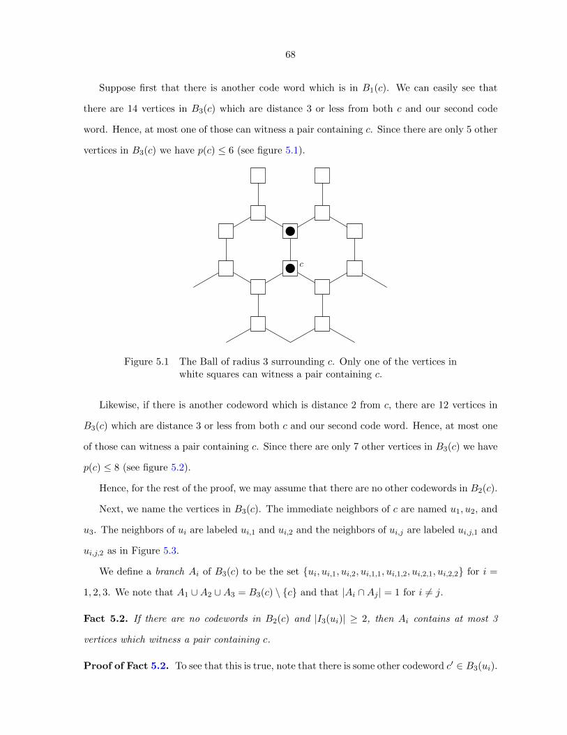
68
Suppose first that there is another code word which is in B1(c). We can easily see that
there are 14 vertices in B3(c) which are distance 3 or less from both c and our second code
word. Hence, at most one of those can witness a pair containing c. Since there are only 5 other
vertices in B3(c) we have p(c) ≤ 6 (see figure 5.1).
c
Figure 5.1 The Ball of radius 3 surrounding c. Only one of the vertices inwhite squares can witness a pair containing c.
Likewise, if there is another codeword which is distance 2 from c, there are 12 vertices in
B3(c) which are distance 3 or less from both c and our second code word. Hence, at most one
of those can witness a pair containing c. Since there are only 7 other vertices in B3(c) we have
p(c) ≤ 8 (see figure 5.2).
Hence, for the rest of the proof, we may assume that there are no other codewords in B2(c).
Next, we name the vertices in B3(c). The immediate neighbors of c are named u1, u2, and
u3. The neighbors of ui are labeled ui,1 and ui,2 and the neighbors of ui,j are labeled ui,j,1 and
ui,j,2 as in Figure 5.3.
We define a branch Ai of B3(c) to be the set {ui, ui,1, ui,2, ui,1,1, ui,1,2, ui,2,1, ui,2,2} for i =
1, 2, 3. We note that A1 ∪A2 ∪A3 = B3(c) \ {c} and that |Ai ∩Aj | = 1 for i 6= j.
Fact 5.2. If there are no codewords in B2(c) and |I3(ui)| ≥ 2, then Ai contains at most 3
vertices which witness a pair containing c.
Proof of Fact 5.2. To see that this is true, note that there is some other codeword c′ ∈ B3(ui).

69
c
Figure 5.2 The Ball of radius 3 surrounding c. Only one of the vertices inwhite squares can witness a pair containing c.
Thus, there is a path of length at most 3 between ui and c′. This path cannot go through c, since
then d(c, c′) ≤ 2, contradicting the fact that there are no other code words in B2(c). Hence,
without loss of generality, we may assume the path goes through ui,2. Thus, d(u1,2, c′) ≤ 2 and
so d(u1,2,i, c′) ≤ 3 for i = 1, 2. Hence, at most one of the vertices in S = {ui, ui,2, ui,2,1, ui,2,2}
can witness a pair containing c. If none of these witness pairs containing c, then our claim is
finished, hence assume that v witnesses a pair containing c for some v ∈ S.
We need to show that one of ui,1, ui,1,1, and ui,1,2 does not witness a pair containing c. By
a symmetric argument, we see that if there is path of length at most 3 through ui,1 between
ui and some other code word c′′, then at most one of ui, ui,1, ui,1,1, ui,1,2 can witness a pair
containing c and so there are at most 2 vertices which witness a pair containing c in Ai. But
now we see that B3(u1,1) ⊂ B3(ui) ∪ B3(u1,1,1) ∪ B3(u1,1,2). Hence, if ui,1 witnesses a pair
containing c this path cannot go through ui (or that codeword is in B3(ui)). So the path goes
through either ui,1,1 or ui,1,2 and thus that vertex cannot witness a pair containing c. Hence,
there can be at most 3 pairs in Ai. This concludes the proof of Fact 5.2. �
We already know that if there are any code words in B2(c), then p(c) ≤ 8 and so we are
only left with the cases where there is there is a codeword in B3(c) \ B2(c) or there are no
other codewords in B3(c).
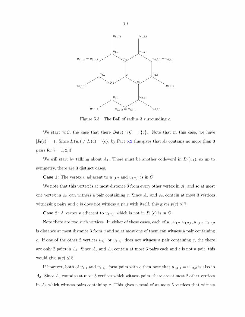
70
c
u1
u2u3
u1,1 u1,2
u2,1
u2,2u3,1
u3,2
u1,1,2 u1,2,1
u2,2,1
u2,1,2
u3,1,2
u3,2,1
u2,2,2 = u3,1,1
u1,1,1 = u3,2,2 u1,2,2 = u2,1,1
Figure 5.3 The Ball of radius 3 surrounding c.
We start with the case that there B3(c) ∩ C = {c}. Note that in this case, we have
|I3(c)| = 1. Since Ir(ui) 6= Ir(c) = {c}, by Fact 5.2 this gives that Ai contains no more than 3
pairs for i = 1, 2, 3.
We will start by talking about A1. There must be another codeword in B3(u1), so up to
symmetry, there are 3 distinct cases.
Case 1: The vertex v adjacent to u1,1,2 and u1,2,1 is in C.
We note that this vertex is at most distance 3 from every other vertex in A1 and so at most
one vertex in A1 can witness a pair containing c. Since A2 and A3 contain at most 3 vertices
witnessing pairs and c is does not witness a pair with itself, this gives p(c) ≤ 7.
Case 2: A vertex v adjacent to u1,2,1 which is not in B3(c) is in C.
Note there are two such vertices. In either of these cases, each of u1, u1,2, u1,2,1, u1,1,2, u1,2,2
is distance at most distance 3 from v and so at most one of them can witness a pair containing
c. If one of the other 2 vertices u1,1 or u1,1,1 does not witness a pair containing c, the there
are only 2 pairs in A1. Since A2 and A3 contain at most 3 pairs each and c is not a pair, this
would give p(c) ≤ 8.
If however, both of u1,1 and u1,1,1 form pairs with c then note that u1,1,1 = u3,2,2 is also in
A3. Since A3 contains at most 3 vertices which witness pairs, there are at most 2 other vertices
in A3 which witness pairs containing c. This gives a total of at most 5 vertices that witness

71
pairs containing c in A1 and A3 and since A2 contains at most 3 pairs, p(c) ≤ 8.
Case 3: The vertex v adjacent to u1,2,2 which is not in B3(c) is in C.
First, assume that u1 does not witness a pair containing c.
Let w be the vertex adjacent to u1,1,1 which is not in B3(c). If w is in C then we see
that u1,2, u1,2,1, and u1,2,2 are all within distance 2 of v so at most one of them can witness
a pair. Likewise, u1,1, u1,1,1, and u1,1,2 are all within distance 2 of w so at most one of them
can witness a pair containing c. Since u1 does not witness a pair, this gives at most 2 vertices
witnessing pairs in A1. As in the other cases, this gives p(c) ≤ 8.
If one of the other vertices in B3(u1) is a codeword, then we are in either Case 1 or Case 2
again, so p(c) ≤ 8. Thus, we may assume that u1 witnesses a pair containing c.
We now wish to turn our attention to A2. Note that u2, u2,1, u2,1,1 and u2,1,2 are all within
distance 2 of v. Thus, none of them can witness pairs containing c. This leaves us with only
u2,2, u2,2,1, and u2,2,2 which could witness pairs containing c. However, note that
B3(u2,2) ⊂ B3(c) ∪B3(u2,2,1) ∪B3(u2,2,2).
Since B3(c) contains no codewords other than c, any codeword in B3(u2,2) must also be in
either B3(u2,2,1) or B3(u2,2,2) and so all 3 of them can’t witness pairs containing c. Thus, A2
contains at most 2 vertices witnessing pairs with c and so p(c) ≤ 8.
This concludes the case where there are no other codewords in B3(c).
We now only have to consider the case where there is a codeword in B3(c) \ B2(c). Up to
symmetry, there are only 2 distinct cases to consider.
Case 1: u2,2,2 ∈ C.
We partition B3(c) into sets as follows:

72
S0 = {c, u2,2,2, u3,1, u3,1,2, u3, u3,2, u2,2, u2, u2,1, u2,1,2}
S1 = {u1,1, u1,1,1, u1,1,2}
S2 = {u1,2, u1,2,1, u1,2,2}
S3 = {u1}
S4 = {u3,2,1, u2,2,1}
Note that each vertex in S0 is within distance 3 of u2,2,2 and so at most one of them can
witness a pair containing c.
In S1 we see that B3(u1,1) ⊂ B3(u1,1,1) ∪ B3(u1,1,2) ∪ B2(c). Since we are assuming that
there are no code words in B2(c) any codeword within distance 3 of u1,1,1 is also within distance
3 of one of the other 2 codewords in S1. Hence, not all 3 can witness pairs containing c and so
at most 2 vertices in S1 form pairs with c.
A symmetric argument shows that at most 2 vertices in S2 can witness pairs containing c.
Next, we consider the lone vertex u1 in S3. Suppose that it witnesses a pair containing
c. Then there is some vertex c′ ∈ C such that there is a path between u1 and c′ which is
of distance less than 3. If the path goes through c, then c′ ∈ B2(c) which is a contradiction.
Thus, the path goes through either u1,1 or u1,2. If it goes through u1,1 then c′ ∈ B2(u1,1) and
hence in B3(v) for all v ∈ S1 and so nothing in S1 can witness a pair containing c. Likewise,
if the path goes through u1,2, nothing in S2 can witness a pair containing c. Totalling this up
we see that there is at most 1 vertex in S0 which can witness a pair containing c, 2 vertices in
S1 ∪ S2, and the three remaining vertices in S3 and S4 which can witness pairs containing c.
This gives p(c) ≤ 6.
If u1 does not witness a pair containing c then we have at most 1 vertex in S0 which
witnesses a pair containing c, 2 vertices in each of S1 and S2 which witness pairs containing c,
and the two remaining vertices in S4 which can witness pairs containing c. This gives p(c) ≤ 7.
Case 2: u1,2,1 ∈ C

73
This case runs basically the same way as the first case. We partition B3(c) into sets:
S0 = {c, u1,2,1, u1,1,2, u1,1, u1, u1,2, u1,2,2, u2,1}
S1 = {u3,2, u3,2,1, u3,2,2}
S2 = {u3,1, u3,1,1, u3,1,2}
S3 = {u2, u2,2, u2,2,1, u2,1,2}
S4 = {u3}
Each vertex in S0 is within distance 3 of u1,2,1 and so at most one of them can witness a
pair containing c.
Using an argument similar to the one we used for S1 in the first case, we see that at most
2 vertices in S1 and S2 can witness pairs containing c.
In S3, we see that B3(u2) ⊂ B3(u2,2) ∪ B3(u2,2,1) ∪ B3(u2,1,2) ∪ B2(c). Similarly to the
argument used for S1 in the first case, we see that at most 3 of the 4 vertices in this set can
witness pairs containing c.
Now considering the lone vertex u3 ∈ S4, we see that if u3 witnesses a pair containing c,
then there is a path to some c′ ∈ C and that path must run through either u3,2 or u3,1. Thus,
there can be no vertices witnessing pairs in S1 or S2 respectively. This gives a max of one
vertex forming a pair in S0, 2 vertices witnessing pairs in S1 ∪ S2, 3 vertices witnessing pairs
in S3 and one vertex witnessing a pair in S4 and so p(c) ≤ 7.
If u3 does not witness a pair containing c, then there is a max of one vertex witnessing a
pair in S0, 2 vertices witnessing pairs in each of S1 and S2, and 3 vertices witnessing pairs in
S3 and so p(c) ≤ 8.
Corollary 5.3. The minimum density of a 3-identifying code of the hex grid is at least 3/25.
Proof. Since b3 = 19 in the hexagonal grid and k ≤ 8 by Lemma 5.1, we get
D(C) ≥ 6
2b3 + 4 + k=
3
25.

74
5.2 A Lower Bound for (r,≤ 2)-Identifying Codes
Lemma 5.4. For an (r,≤ 2)-identifying code of the Hexagonal grid, there must be 5 codewords
in the region Br+1(v) \Br−1(v) for any vertex v.
Proof. Let S = Br+1(v) \Br−1(v) and let Sx = S ∩Br(x). Let u1, u2, and u3 be the neighbors
of v. We see that Br(v) ∩Br(u1) ∩Br(u2) ∩Br(u3) = Br−1(v) and likewise, Br(v) ∪Br(u1) ∪
Br(u2) ∪Br(u3) = Br+1(v). Hence, Ir(S1)4Ir(S2) ⊂ S for Si ⊂ {v, u1, u2, u3}, |Si| ≤ 2.
We will show that 4 codewords is not enough to distinguish between all S ⊂ {v, u1, u2, u3},
|S| ≤ 2.
Suppose that {c1, c2, c3, c4} ∩ S = C ∩ S. Let
K(X) =
(⋃x∈X
Sx
)∩ C.
We write K({x1, . . . , xn}) = K(x1, . . . , xn) for short. It is clear that our code can only be valid
if K(X) 6= K(Y ) for X,Y ⊂ {v, u1, u2, u3} with X 6= Y and |X|, |Y | ≤ 2.
Fact 1: For x, y ∈ {v, u1, u2, u3} with x 6= y, if K(x) ⊂ K(y), then C is not an (r,≤ 2)-
identifying code.
Proof. K(y) = K(x, y) and so C is not an (r,≤ 2)-identifying code.
Fact 2: If c ∈ K(v) then c ∈ K(ui) for some i.
Proof. The fact is immediate since Br(v) ⊂⋃3
i=1Br(ui).
Case 1: There are three or more code words in Sui for some i.
Without loss of generality, assume that {c1, c2, c3} ⊂ Su1 . If c4 6∈ Su2 , then K(u2) ⊂ K(u1)
and so C is not an (r,≤ 2)-identifying code. Hence, c4 ∈ Su2 and by a symmetric argument,
c4 ∈ Su3 . But then K(u1, u2) = K(u1, u3) = {c1, c2, c3, c4}. Hence, |K(ui)| ≤ 2 for each i.
Case 2: There are two codewords in Sui ∩ Suj for i 6= j.
75
Assume again without loss of generality that Su1 ∩ Su2 = {c1, c2}. From case 1, there can
be no other codewords in Su1 or Su2 and so K(u1) = K(u2) = {c1, c2}. Hence |Sui ∩ Suj | ≤ 1
for i 6= j.
Case 3: Sui ∩ Suj = ∅ for i 6= j.
From the above cases, we must have 2 code words in 1 component and 1 in the other two.
Hence, we may assume K(u1) = {c1, c2}, K(u2) = {c3}, and K(u3) = {c4}.
If c3 ∈ K(v), then K(u2) ⊂ K(v) and so c3 6∈ K(v). Likewise, c4 6∈ K(v). But then
K(v) ⊂ {c1, c2} = K(u1, u2).
Case 4: |Sui ∩ Suj | = 1 for some i 6= j.
Assume without loss of generality that c1 ∈ K(u1)∩K(u2). If K(u1) = {c1} then K(u1) ⊂
K(u2) and so there must be at least one more code word in K(u1). But from case 1, |K(u1)| ≤ 2
and so assume that K(u1) = {c1, c2} and likewise, we may assume that K(u2) = {c1, c3}. Since
Su1∩Su2∩Su3 = ∅ we must have c1 6∈ Su3 and since Su1∪Su2∪Su3 = S, we must have c4 ∈ Su3 .
If K(u3) = {c4}, then c4 6∈ K(v) as in case 3. If c2 6∈ K(v) then K(v) ⊂ {c1, c3} = K(u2),
hence c2 ∈ K(v). But then K(v, u2) = K(u1, u2) = {c1, c2, c3}.
Hence, we must have one of c2 and c3 in Su3 , but we cannot have both or else we are in case
1. So without loss of generality, assume K(u3) = {c2, c4}. If |K(v)| = 1 then K(v) ⊂ K(ui)
for some i. Hence, |K(v)| > 1. We already have
K(u1) = {c1, c2}
K(u2) = {c1, c3}
K(u3) = {c2, c4}
K(u1, u2) = {c1, c2, c3}
K(u1, u3) = {c1, c2, c4}
K(u2, u3) = {c1, c3, c3, c4}
which leaves only 5 possible combinations for K(v). We enumerate them here and show that

76
each case causes a contradiction.
K(v) Contradiction
{c1, c4} K(u1, u3) = K(u1, v) = {c1, c2, c4}
{c2, c3} K(u1, u2) = K(u1, v) = {c1, c2, c3}
{c3, c4} K(u2, u3) = K(u1, v) = {c1, c2, c3, c4}
{c1, c3, c4} K(u2, u3) = K(u1, v) = {c1, c2, c3, c4}
{c2, c3, c4} K(u2, u3) = K(u1, v) = {c1, c2, c3, c4}
Theorem 5.5. The minimum density of an (r,≤ 2)-identifying code in the hex grid is at least
5
6r + 3.
Proof. We refer to the methods of Charon, Honkala, Hudry and Lobstein [3] used to prove
a minimum density for (r,≤ 1)-identifying codes for various infinite grids. Since |Br+1(v) \
Br−1(v)| = 6r + 3 [5] for any v ∈ V (GH) and Br+1(v) \ Br−1(v) must contain at least 5 code
words by the previous lemma, any code must have density at least5
6r + 3.
77
CHAPTER 6. VERTEX IDENTIFYING CODES FOR REGULAR
GRAPHS
6.1 Introduction
We wish to improve and expand upon some of the ideas mentioned in the introduction.
In particular, we want to look at the densities of codes on graphs that are dense with edges.
We first focus on improving the general lower bound for such graphs with the theorems in
Section 6.2 and then construct regular (or near regular) graphs that have codes attaining this
lower bound in Section 6.4.
6.2 Theorems
We start by presenting lower bounds or the size of regular graph codes.
Theorem 6.1. Let C be an identifying code in an n vertex graph G with maximum degree ∆.
Then
|C| ≥ max
{2n
∆ + 2,−(2∆ + 5) +
√(2∆ + 5)2 + 24n
2
}Theorem 6.2. Let C be an identifying code in an n vertex graph G with maximum degree ∆.
Then
|C| ≥ max1≤s≤∆
{(s+ 1)n
∆ + 1
[1− (s+ 1)s−2ns−1
s!(∆ + 1)s
]}
6.3 Proofs
Recall Theorem 1.12 which shows that for a d-regular graph the minimum size of a vertex
identifying code
|C| ≥ 2n
d+ 2.

78
This is done by a double counting argument in which we count the size of the identifying sets
as well as the ball of radius 1 surrounding each codeword. We note that this bound holds for
the code of any graph of maximum degree ∆ as well. We then generalize this argument to get
better bounds.
Proof of Theorem 6.1.
Proof. Recall the equationk∑
j=1
|Br(cj)| =∑
v∈V (G)
|Ir(v)|. (6.1)
If we have k codewords, then we can upper bound the left hand side by (∆ + 1)k.
If n ≥ k +(k2
), then note that we have at most k identifying sets of size k,
(k2
)identifying
sets of size 2 and so the rest of our identifying sets have size at least 3. Thus, we can lower
bound the right hand size by
k + 2
(k
2
)+ 3
[n− k −
(k
2
)]and so
(∆ + 1)k ≥ k + 2
(k
2
)+ 3
[n− k −
(k
2
)]. (6.2)
Solving for k gives
k ≥−(2∆ + 5) +
√(2∆ + 5)2 + 24n
2
However, suppose that n < k +(k2
). From Karpovsky, we already know that any code
satisfies (∆ + 1)k ≥ 2n− k. But then
(∆ + 1)k ≥ 2n− k
≥ 2n− k +
[n− k −
(k
2
)]= k + 2
(k
2
)+ 3
[n− k −
(k
2
)]and so k satisfies equation (6.2) anyway and
|C| ≥ max
{2n
∆ + 2,−(2∆ + 5) +
√(2∆ + 5)2 + 24n
2
}.

79
Next, define the function
f(n, k, s) =
s∑i=1
i
(k
i
)+ (s+ 1)
[n−
s∑i=1
(k
i
)].
We will use this function in the proof of theorem 6.2 so we first present a quick lemma.
Lemma 6.3. f(n, k, s) = f(n, k, s− 1) + n−∑s
i=1
(ki
)Proof. The result follows by simple algebraic manipulation.
f(n, k, s) =s∑
i=1
i
(k
i
)+ (s+ 1)
[n−
s∑i=1
(k
i
)]
=s−1∑i=1
i
(k
i
)+ s
[n−
s−1∑i=1
(k
i
)]+ n−
s∑i=1
(k
i
)
= f(n, k, s− 1) + n−s∑
i=1
(k
i
)
Lemma 6.4. Suppose a graph G with maximum degree ∆ has a code of size k. Then k satisfies
(∆ + 1)k ≥ f(n, k, s) (6.3)
for 1 ≤ s ≤ ∆.
Proof. Here we generalize the argument from Theorem 6.1. For any s ≥ 1, if n ≥∑s
i=1
(ki
),
then
(∆ + 1)k ≥s∑
i=1
i
(k
i
)+ (s+ 1)
[n−
s∑i=1
(k
i
)]= f(n, k, s)
which follows from bounding both sides of Equation 6.1. The left hand side is at most (∆+1)k
and for the right hand side, we have at most(ki
)identifying sets of size i for 1 ≤ i ≤ s. Let s∗
be the largest s for which n ≥∑s
i=1
(ki
)holds. Then for any s ≥ s∗ we have n−
∑si=1
(ki
)< 0.
So,
(∆ + 1)k ≥ f(n, k, s)
≥ f(n, k, s) + n−s+1∑i=1
(k
i
)= f(n, k, s+ 1).
Hence, we have (∆ + 1)k ≥ f(n, k, s∗ + r) for any r ≥ 0.
80
Proof of Theorem 6.2.
Proof. First we note that
f(n, k, s) =
s∑i=1
i
(k
i
)+ (s+ 1)
[n−
s∑i=1
(k
i
)]
= (s+ 1)n−s∑
i=1
i
(k
i
)+
s∑i=1
(s+ 1)
(k
i
)
= (s+ 1)n+
s∑i=1
(s+ 1− i)(k
i
).
From Lemma 6.4, we know that a code of size k satisfies (∆+1)k ≥∑k
i=1(d(ci)+1) ≥ f(n, k, s)
so this gives
(∆ + 1)k ≥ (s+ 1)n+s∑
i=1
(s+ 1− i)(k
i
)≥ (s+ 1)n− s
(k
s
)≥ (s+ 1)n− ks
(s+ 1)!
and so
n(s+ 1)(s+ 1)! ≤ ks + (s+ 1)!k(∆ + 1).
Next note that if
k >(s+ 1)n
∆ + 1
then the hypothesis of our theorem are already satisfied. Hence, we may assume that
k ≤ (s+ 1)n
∆ + 1.
Next, let
k = (1− ε)(s+ 1)n
∆ + 1≤ (s+ 1)n
∆ + 1

81
Then we can plug this into the expression above to get
n(s+ 1)(s+ 1)! ≤ ks + (s+ 1)!k(∆ + 1)
n(s+ 1)(s+ 1)! ≤(
(s+ 1)n
∆ + 1
)s
+ (s+ 1)!(1− ε)(s+ 1)n
ε(s+ 1)(s+ 1)!n ≤(
(s+ 1)n
∆ + 1
)s
ε ≤ (s+ 1)s−1ns−1
(s+ 1)!(∆ + 1)s
and hence
1− ε ≥ 1− (s+ 1)s−1ns−1
(s+ 1)!(∆ + 1)s
(1− ε)(s+ 1)n
∆ + 1≥ (s+ 1)n
∆ + 1
[1− (s+ 1)s−2ns−1
s!(∆ + 1)s
]k ≥ (s+ 1)n
∆ + 1
[1− (s+ 1)s−2ns−1
s!(∆ + 1)s
].
6.4 Construction of Graphs Satisfying the Bounds
Let k be given and s+ 1 ≤ k. We then construct a graph of order n =∑s+1
i=1
(ki
)and max
degree ∆ =∑s+1
i=2
(k−1i−1
)satisfying (6.3).
Let C be a set of k vertices. For i = 2, . . . , s+ 1 let Ci be a set of(ki
)vertices. Then there
is a bijection ϕ : Ci →(Ci
). So for each vertex v ∈ Ci, we create an edge between v and each
vertex in ϕ(v).
The degree of a vertex in Ci, i ≥ 2 is exactly i. Then, for each vertex in C, it is adjacent
to 1 vertex in Ci for each subset of size i− 1 of the remaining k− 1 vertices and so the degree
of a vertex in C is exactly ∆ =∑s+1
i=2
(k−1i−1
).
Now we claim that C is a code. For each vertex in c ∈ C, it is not adjacent to any other
vertex in C and so N [c] ∩ C = {c} and for each vertex in Ci, it is adjacent to a unique subset
of size i. Hence, N [v] ∩ C is unique for every vertex in our graph. Note that in this case we
have exact equality in equation (6.3).
Of particular interest are graphs that are regular or almost regular. Note that if you create
a graph in the fashion described above, that C will still be a code if you add edges between

82
any two vertices not in C since N [v]∩C remains unchanged for each vertex when these edges
are added.
Theorem 6.5. Let k = 3t + 2 and t ≡ 1 or 2 (mod 4). There exists a d regular graph on n
vertices admitting a 1-identifying code of size
−(2d+ 5) +√
(2d+ 5)2 + 24n
2
where d =(k2
)and n = k +
(k2
)+(k3
).
Proof. Create a regular graph in the method described above with s = 2 and k = 3t+ 2. Then
we have d =(k−1
1
)+(k−1
2
)=(k2
). Next, the degree of each vertex in C2 is currently 2. So if
we connect each pair of vertices with an edge they will have degree(k2
)+ 1. However, under
our conditions for k,(k2
)will be even so we then remove a matching and each vertex with then
have degree d.
Finally, there are(k3
)= k−2
3
(k2
)vertices in C3. Since k−2
3 = t is an integer, we can partition
it into t sets of(k2
)vertices and turn each of those into a complete graph and then remove a
Hamiltonian cycle from each of them so that each vertex in C3 now has degree d as well.
We next wish to show the existence of arbitrarily large graphs that attain equality in
equation (6.3) for higher values of s.
Theorem 6.6. For all k, s ≥ 2, there exists a graph on n vertices which is either d-regular or
that has n − 1 vertices of degree d and 1 vertex of degree d − 1 that admits a code of size k
where
d =
s+1∑i=2
(k − 1
i− 1
)and
n =s+1∑i=1
(k
i
).
Before proving the theorem, we need a technical lemma.
83
Lemma 6.7. Let k be given and s ≤ k − 1 and define m =∑s+1
i=2
(ki
)and d =
∑s+1i=2
(k−1i−1
).
Then there exists a graph of degree sequence
(d− 2, . . . , d− 2︸ ︷︷ ︸(k2) times
, d− 3, . . . , d− 3︸ ︷︷ ︸(k3) times
, . . . , d− (s+ 1), . . . , d− (s+ 1)︸ ︷︷ ︸( ks+1) times
)
if the sums of the degrees is even. If the sum of the degrees in the above sequence is odd, there
exists a graph of the degree sequence above, replacing the last d− 2 with d− 3.
Proof. By the Erdos-Gallai Theorem[16], we know that a graph with this degree sequence
exists if the sum of the degrees in the sequence is even and
r∑i=1
di ≤ r(r − 1) +
m∑i=r+1
min(di, r) (6.4)
for all 1 ≤ r ≤ m. From the statement of the lemma, it is clear that our sequence is even.
Next, assuming the convention that(nk
)= 0 if k > n, we note that
m =s+1∑i=2
(k
i
)=
s+1∑i=2
[(k − 1
i− 1
)+
(k − 1
i
)]= d+
s+1∑i=2
(k − 1
i
)also, we have
m = 2d+
(k − 1
s+ 1
)−(k − 1
1
).
Dealing with the left hand side of Inequality 6.4, note that∑r
i=1 di ≤ r(d − 2). For the
right hand side, we break into 3 cases.
Case 1: r ≤ d− s− 1
Then
r(r − 1) +
m∑i=r+1
min(di, r) = r(r − 1) +
m∑i=r+1
r
= r(r − 1) + (m− r)r
= r(m− 1)
≥ r(d− 2)
Where the last step holds since d < m.
84
Case 2: r ≥ d− 2
Then
r(r − 1) +m∑
i=r+1
min(di, r) ≥ r(r − 1)
≥ r(d− 2)
Case 3: d− s− 1 < r < d− 2
For the left hand side, we now have
r∑i=1
di ≤ r(d− 2) ≤ (d− 2)2
and the right hand side becomes
r(r − 1) +m∑
i=r+1
min(di, r) = r(r − 1) +m∑
i=r+1
d− s− 2
≥ r(d− s− 2) + (m− r)(d− s− 2)
= m(d− s− 2)
≥(
2d+
(k − 1
s+ 1
))(d− s− 2)
Thus, we turn our attention to showing that
(d− 2)2 ≤(
2d+
(k − 1
s+ 1
))(d− s− 2).
After algebraic manipulation, we rewrite this as
d(d− 2s)− 4 +
(k − 1
s+ 1
)(d− s− 2) ≥ 0.
The last term is clearly positive and we note that d(d− 2s)− 4 is positive if d ≥ 2s+ 1 and
d ≥ 4. To show the first inequality, first note that s ≥ 2. Then
d ≥(s
1
)+
(s
2
)= s+ (s2 + s)/2.
Then through simple algebraic manipulation we see that d ≥ s+ (s2 + s)/2 ≥ 2s+ 1 as long as
s ≥ 2. The second inequality then immediately follows from the first since d ≥ 2s+ 1 ≥ 4.

85
Proof of Theorem 6.6. Again, create a graph G on n vertices with a code of size k as
described earlier. Each vertex in Ci currently has degree i. Thus, we wish to create a graph
on C2 ∪ C3 ∪ · · · ∪ Cs+1 such that each vertex in Ci has degree d− i. This is impossible if the
sums of the degrees is odd, but in Lemma 6.7, we showed that it is possible to find a graph
that has the proper degree sequence or with at most one vertex being one degree d− i− 1.
Then, by Lemma 6.7 we may create a graph on C2 ∪C3 ∪ · · · ∪Cs+1 such that each vertex
in Ci has degree d− i or all but one vertex does and the remaining vertex has degree d− i− 1.
Superimposing this on our graph G gives the desired result. �
86
Bibliography
[1] Yael Ben-Haim and Simon Litsyn. Exact minimum density of codes identifying vertices
in the square grid. SIAM J. Discrete Math., 19(1):69–82, 2005.
[2] Uri Blass, Iiro Honkala, and Simon Litsyn. On binary codes for identification. J. Combin.
Des., 8(2):151–156, 2000.
[3] Irene Charon, Iiro Honkala, Olivier Hudry, and Antoine Lobstein. General bounds for
identifying codes in some infinite regular graphs. Electron. J. Combin., 8(1):Research
Paper 39, 21 pp. (electronic), 2001.
[4] Irene Charon, Iiro Honkala, Olivier Hudry, and Antoine Lobstein. The minimum density
of an identifying code in the king lattice. Discrete Math., 276(1-3):95–109, 2004.
[5] Irene Charon, Olivier Hudry, and Antoine Lobstein. Identifying codes with small radius
in some infinite regular graphs. Electron. J. Combin., 9(1):Research Paper 11, 25 pp.
(electronic), 2002.
[6] Irene Charon, Olivier Hudry, and Antoine Lobstein. Possible cardinalities for identifying
codes in graphs. Australas. J. Combin., 32:177–195, 2005.
[7] Irene Charon, Olivier Hudry, and Antoine Lobstein. Extremal cardinalities for identifying
and locating-dominating codes in graphs. Discrete Math., 307(3-5):356–366, 2007.
[8] Gerard Cohen, Iiro Honkala, Simon Litsyn, and Antoine Lobstein. Covering codes, vol-
ume 54 of North-Holland Mathematical Library. North-Holland Publishing Co., Amster-
dam, 1997.

87
[9] Gerard Cohen, Iiro Honkala, Antoine Lobstein, and Gilles Zemor. New bounds for codes
identifying vertices in graphs. Electron. J. Combin., 6:Research Paper 19, 14 pp. (elec-
tronic), 1999.
[10] Gerard Cohen, Iiro Honkala, Antoine Lobstein, and Gilles Zemor. Bounds for codes iden-
tifying vertices in the hexagonal grid. SIAM J. Discrete Math., 13(4):492–504 (electronic),
2000.
[11] Gerard Cohen, Iiro Honkala, Michel Mollard, Sylvain Gravier, Antoine Lobstein, Charles
Payan, and Gilles Zemor. Improved identifying codes for the grid. Electron. J. Combin.,
6:Research Paper 19, Comment, 3 pp. (electronic), 1999.
[12] Gerard D. Cohen, Iiro Honkala, Antoine Lobstein, and Gilles Zemor. On codes identifying
vertices in the two-dimensional square lattice with diagonals. IEEE Trans. Comput.,
50(2):174–176, 2001.
[13] Gerard D. Cohen, Iiro Honkala, Antoine Lobstein, and Gilles Zemor. On identifying codes.
In Codes and association schemes (Piscataway, NJ, 1999), volume 56 of DIMACS Ser.
Discrete Math. Theoret. Comput. Sci., pages 97–109. Amer. Math. Soc., Providence, RI,
2001.
[14] Daniel W. Cranston and Gexin Yu. A new lower bound on the density of vertex identifying
codes for the infinite hexagonal grid. Electron. J. Combin., 16(1):Research Paper 113, 16,
2009.
[15] Ari Cukierman and Gexin Yu. New bounds on the minimum density of a vertex identifying
code for the infnite hexagonal grid. Submitted.
[16] Paul Erdos and Tibor Gallai. Grafok eloırt fokszamu pontokkal. Matematikai Lapok,
11:264–274, 1960 (Hungarian).
[17] Florent Foucaud, Eleonora Guerrini, Matjaz Kovse, Reza Naserasr, Aline Parreau, and
Petru Valicov. Extremal graphs for the identifying code problem. European Journal of
Combinatorics, 32(4):628–638, 2011.

88
[18] Alan Frieze, Ryan Martin, Julien Moncel, Miklos Ruszinko, and Cliff Smyth. Codes
identifying sets of vertices in random networks. Discrete Math., 307(9-10):1094–1107,
2007.
[19] Iiro Honkala. An optimal strongly identifying code in the infinite triangular grid. Electron.
J. Combin., 17(1):Research Paper 91, 10, 2010.
[20] Iiro Honkala, Mark G. Karpovsky, and Lev B. Levitin. On robust and dynamic identifying
codes. IEEE Trans. Inform. Theory, 52(2):599–612, 2006.
[21] Iiro Honkala and Tero Laihonen. Codes for identification in the king lattice. Graphs
Combin., 19(4):505–516, 2003.
[22] Iiro Honkala and Tero Laihonen. On the identification of sets of points in the square
lattice. Discrete Comput. Geom., 29(1):139–152, 2003.
[23] Iiro Honkala and Tero Laihonen. On identifying codes in the triangular and square grids.
SIAM J. Comput., 33(2):304–312 (electronic), 2004.
[24] Iiro Honkala and Tero Laihonen. On identifying codes that are robust against edge
changes. Inform. and Comput., 205(7):1078–1095, 2007.
[25] Iiro Honkala, Tero Laihonen, and Sanna Ranto. On strongly identifying codes. Discrete
Math., 254(1-3):191–205, 2002.
[26] Iiro Honkala and Antoine Lobstein. On the density of identifying codes in the square
lattice. J. Combin. Theory Ser. B, 85(2):297–306, 2002.
[27] Ville Junnila and Tero Laihonen. Optimal lower bound for 2-identifying code in the
hexagonal grid. Electron. J. Combin., Submitted.
[28] G. A. Kabatyanskiı and V. I. Panchenko. Packings and coverings of the Hamming space
by unit balls. Dokl. Akad. Nauk SSSR, 303(3):550–552, 1988.
[29] Mark G. Karpovsky, Krishnendu Chakrabarty, and Lev B. Levitin. On a new class of codes
for identifying vertices in graphs. IEEE Trans. Inform. Theory, 44(2):599–611, 1998.
89
[30] Tero Laihonen. Optimal codes for strong identification. European J. Combin., 23(3):307–
313, 2002.
[31] Tero Laihonen. On optimal edge-robust and vertex-robust (1,≤ l)-identifying codes. SIAM
J. Discrete Math., 18(4):825–834 (electronic), 2005.
[32] Tero Laihonen and Sanna Ranto. Codes identifying sets of vertices. In Applied algebra,
algebraic algorithms and error-correcting codes (Melbourne, 2001), volume 2227 of Lecture
Notes in Comput. Sci., pages 82–91. Springer, Berlin, 2001.
[33] Antoine Lobstein. Internet bibliography.
http://www.infres.enst.fr/~lobstein/bibLOCDOMetID.html.
[34] Ryan Martin and Brendon Stanton. On improved lower bounds for identifying codes in
the square and hexagonal grids. Electron. J. Combin., 17(1):Research Paper 122, 16 pp.
(electronic), 2010.
[35] Julien Moncel. On graphs on n vertices having an identifying code of cardinality dlog2(n+
1)e. Discrete Appl. Math., 154(14):2032–2039, 2006.
[36] Douglas F. Rall and Peter J. Slater. On location-domination numbers for certain classes
of graphs. In Proceedings of the fifteenth Southeastern conference on combinatorics, graph
theory and computing (Baton Rouge, La., 1984), volume 45, pages 97–106, 1984.
[37] Miranda L. Roden and Peter J. Slater. Liar’s domination in graphs. Discrete Math.,
309(19):5884–5890, 2009.
[38] Brendon Stanton. On improved upper bounds for identifying codes in the hexagonal grid.
SIAM J. Discrete Math., 25(1):pp. 159–169, 2011.
[39] Brendon Stanton. Vertex identifying codes for the n-dimensional lattice. Discrete Math.,
Submitted.
[40] Douglas B. West. Introduction to graph theory. Prentice Hall Inc., Upper Saddle River,
NJ, 1996.