one-dimensional, ocean surface layer modeling - geophysical

790 VOLUME 31J O U R N A L O F P H Y S I C A L O C E A N O G R A P H Y

q 2001 American Meteorological Society

One-Dimensional, Ocean Surface Layer Modeling: A Problem and a Solution

GEORGE L. MELLOR

Program in Atmospheric and Oceanic Sciences, Princeton University, Princeton, New Jersey

(Manuscript received 19 April 1999, in final form 1 June 2000)

ABSTRACT

The first part of this paper is generic; it demonstrates a problem associated with one-dimensional, oceansurface layer model comparisons with ocean observations. Unlike three-dimensional simulations or thereal ocean, kinetic energy can inexorably build up in one-dimensional simulations, which artificially en-hances mixing. Adding a sink term to the momentum equations counteracts this behavior. The sink termis a surrogate for energy divergence available to three-dimensional models but not to one-dimensionalmodels.

The remainder of the paper deals with the Mellor–Yamada boundary layer model. There exists priorevidence that the model’s summertime surface temperatures are too warm due to overly shallow mixedlayer depths. If one adds a sink term to approximate three-dimensional model behavior, the warming problemis exacerbated, creating added incentive to seek an appropriate model change. Guided by laboratory data,a Richardson-number-dependent dissipation is introduced and this simple modification yields a favorableimprovement in the comparison of model calculations with data even with the momentum sink term inplace.

1. Introduction

This paper is in two parts. The first part, sections 2and 3, is generic. We show that numerical one-dimen-sional simulations of mixed layer behavior should in-clude a sink parameterization to account for energy fluxdivergence that is generally present in the ocean and inthree-dimensional, numerical ocean simulations. With-out an energy sink, wind-driven, surface layer velocitiesgenerated by a one-dimensional model will inexorablyincrease and, in the course of a multimonth simulation,erroneously enhance mixed layer deepening and surfacetemperature cooling. One presumes that this has intro-duced error in past comparisons of one-dimensionalmodel results with observational data. Introducing a mo-mentum sink term is a completely empirical means ofsimulating three-dimensional energy divergence, but isdeemed better than excluding the sink. And Pollard andMillard (1970) did incorporate a sink term in a simplemodel in order to match the model with current meterobservations. Since their paper, the emphasis has beenpredominantly on the prediction of mixed layer tem-peratures and salinities wherein currents were ignored.

Whereas sections 2 and 3 should apply to most mod-els, the second part of the paper focuses on the Mellor-

Corresponding author address: Dr. George L. Mellor, Program inAtmospheric and Oceanic Sciences, Princeton University, BoxCN710, Sayre Hall, Princeton, NJ 08544-0710.E-mail: [email protected]

Yamada (henceforth M–Y) model, which is often usedin atmospheric and ocean general circulation models. Itis not a planetary boundary layer model per se; it is amore general turbulence closure model that happenedto ape quite a few properties of stratified planetaryboundary layers (Mellor 1973; Mellor and Yamada1974, 1982). Other second moment models with appli-cation to geophysical flows include those by Lewellenand Teske (1973), Lumley et al. (1978), Andre and La-carrere (1985), Therry and Lacarrere (1983), and Rodi(1987). The model of Andre and Lacarrere is labeled athird moment model by the authors, since closures areconstructed for the fourth moment terms in an equationfor the diffusional third moments. However, the moreimportant pressure–velocity gradient terms and the dis-sipation related to the gradient of the two-point triplecorrelation are still closed at a lower order so that themodel is predominantly a second moment model. For amore general review of mixed layer models includingeddy viscosity and bulk models, see Kantha and Clayson(1994).

By incorporating model hypotheses and nondimen-sional constants derived from neutral laboratory data,the M–Y model very nearly reproduced the Monin–Obukhov similarity relations for near-surface stratifiedflows, both stable and unstable. However, in applicationto the entire surface boundary layer, the model has beencriticized for overly shallow oceanic surface layerdepths and overly warm, sea surface temperatures dur-ing summertime stable conditions. In particular, Martin

MARCH 2001 791M E L L O R

(1985) showed that summertime temperatures at OceanWeather Station Papa exceeded observations by about28C relative to an annual range of 88C. For this reason,Kantha and Clayson (1994) deemed it necessary toamend the M–Y model and directly add eddy viscosityand diffusivity (thus abandoning a modeling principalthat empirical constants should be nondimensional) tothe base of the mixed layer.

The findings in section 2 and 3 exacerbate the prob-lem since, with the addition of a momentum sink, sum-mertime surface temperatures are increased. Thereforea modification is made to the M–Y model and that isto replace the existing submodel for dissipation with aRichardson number (based on turbulence variables) de-pendent, model dissipation. The need for such a mod-ification was first revealed by a laboratory experimentof decaying, density-stratified turbulence (Dickey andMellor 1980, henceforth DM) wherein the turbulence atfirst decays in approximately classical fashion (turbu-lence kinetic energy } time21) but then, rather abruptly,transitions to a random ensemble of internal waves withvery little decay, an equilibrium state similar to thatoccurring in the ocean (Garrett and Munk 1979). It issomewhat of a jump in parameter space from that ex-periment to the shear-dominated regimes of planetaryboundary layers. Still, one would hope that the modelwould include the DM case. As we will demonstrate,inclusion of a Richardson-number-dependent, energydissipation increases the turbulence kinetic energy inthe outer portion of the layer, increases boundary layerthickness, and improves comparison with observationsusing wind stress and heat flux compiled by Martin(1985).

There are, of course, other sources of disageementbetween model calculations and one-dimensional data.Aside from oversimplication of model physics and dataerrors, they include model finite difference errors, un-known vertical and horizontal advection of observedmean properties, interaction with unknown remotelygenerated internal and surface waves or with baroclinicvelocity shears, and errors or lack of resolution in thesurface forcing data that drive a model.

2. Artificial velocity buildup in one-dimensionalocean surface layer models

Pollard and Millard (1970) adopted a simple oceanmixed layer model:

]u ]tzx2 fy 5 2 cu, (1a)]t ]z

]t]y zy1 fu 5 2 cy , (1b)

]t ]z

wherein the vertical divergence of the wind stress,(]t zx/]z, ]t zy/]z) 5 (t ox, t oy)/h, was distributed uniform-ly over a layer of fixed depth, h, and the velocity com-

ponents, u and y , are independent of depth. Accordingto Pollard and Millard,

The linear damping term models the (three-dimensional)dispersion effect by introducing a decay factor of theform, exp(2ct); c21 is the e-folding time. It should benoted that the damping term has the effect of shifting thedominant frequency response of the model to a frequencyslightly less than f when the frequency spectrum of theforcing is flat. This is not a good property when modelingthe real ocean where inertio–gravity waves have fre-quencies between f and the Brunt–Vaisala frequency N.Since N is usually greater than f, the dominant frequencyobserved is usually slightly greater than f.

Figure 1 is a comparison of the simple model for c21

5 8 inertial days and h 5 45 m, with observationaldata. The point to be made is that this empirical dampingterm was considered important toward improved com-parison with current meter measurements. Other caseswere considered in the paper and various values of cwere chosen to minimize model error.

We wish now to derive somewhat more general resultsrelated to one-dimensional, ocean, surface layer models.To simplify the matter, consider the vertical integrals of(1a,b), which, for zero stress at depth, are

]Sx 2 fS 5 t 2 cS , (2a)y ox x]t

]Sy1 fS 5 t 2 cS , (2b)x oy y]t

where (Sx, Sy) [ ( u dz, y dz) and h, a constant,0 0# #2h 2h

is large enough so that (t2hx, t2hy) 5 (0, 0). The con-ventional Ekman transport is obtained when c 5 0 andthe tendency terms are nil. Equations (2a,b) are an exact,zero-dimensional model, which conveniently excludesconsideration of detailed profile structure.

We have available the 3-hourly wind data used byMartin (1985) at OWS Papa (508N, 1458W) and No-vember (308N, 1408W). These winds are used to nu-merically compute ( , 1 )1/2 from (2a,b) and the2 2S Sx y

results are plotted as solid lines in Figs. 2a,b for c 5 0and c 5 (10 d)21.

Signals from the c 5 0 case increase with time andthis result can also be obtained from integrals of velocityprofiles calculated by the full z-dependent model (seesection 4) if we set h $ 160 m, the depth of maximumpenetration of turbulence kinetic energy, Reynoldsstress, and currents. On the other hand, the signal fromthe c ± case flattens, on average, to constant values.We now show that this behavior is to be expected forsystems such as (2a,b).

3. Statistical expectation

For the present purpose, the winds at Papa and No-vember can be approximated as a random time signalafter the means of (Sx, Sy) 5 f 21(t ox, 2t oy) have been


FIG. 1. Wind record and response of a simple slab model (heavy line) by Pollard and Millard(1970) and compared with current meter measurements (light line) at 39820.59N, 698599W and adepth of 7 m during Oct 1965.

subtracted. Without change in nomenclature and aftersubtracting the means, (2a,b) may be written

]S1 i fS 5 s 2 cS, (3)

]t

where s [ t ox 1 it oy and S [ Sx 1 iSy and i [ (21)1/2.A solution to (3) for resting initial conditions is

T

2(i f1c)T (i f1c)tS(T ) 5 e e s(t) dt. (4)E0

a. Expected behavior with no decay

In Eq. (4), let c 5 0. If now we write the modulussquared of S, we obtain

T T

i f (t 2t )1 2SS* 5 e s(t )s*(t ) dt dt ,E E 1 2 1 2

0 0

where the overbars denote ensemble means and an as-terisk denotes a complex conjugate. Now let t2 [ t 1t /2, t1 [ t 2 t /2, and s(t1)s*(t2) 5 Rs(t) 5 Rs(2t).After some manipulation (Taylor 1921), we obtain

T

SS* 5 2 (T 2 t)R (t) cos ft dt . (5)E s

0

For small T compared to the decorrelation time, SS* 5T 2Rs(0), whereas for large T

`

SS* 5 2T cos ftR (t) dt . (6)E s

0

Wind stress correlations have been obtained from theyearlong records for stations Papa and November (cour-tesy P. Martin) and are plotted in Fig. 3. An approxi-mation to Rs(t) is Rs(0)e2a|t | after which the quadraturein (6) may be evaluated such that Rs(t) cos ft dt 5`#0

Rs(0)a/(a2 1 f 2). This result plus the values, Rs(0) anda, obtained from Fig. 3, provide the dashed lines in Figs.2a and 2b wherein (SS*)1/2 } T 1/2. Note that one shouldideally compare the average of an ensemble of data withthe statistical model. Nevertheless, there is little doubtthat the statistical model explains the behavior of thetwo experiments in that a one-dimensional Ekman layervelocities, forced by a wind, approximated by a randomprocess, will inexorably increase.


FIG. 2. The growth of Ekman transport for (a) OWS Papa and (b) OWS November. The solid lines arenumerical solutions of Eqs. (2a,b) where the dashed lines are obtained from (6) and (7). In each diagramthe upper curves are for c 5 0 whereas the lower curves are for c 5 (10 d)21.

b. Expected behavior with decay

We now repeat the analysis for c ± 0 and obtain

`

21 2ctSS* 5 c e cos ftR (t) dt (7)E s

0

for large T instead of (6). With the exponential approx-imation for Rs(t) noted above, Rs(t)e2ct cos ft dt`#0

5 Rs(0)(a 1 c)/[(a 1 c)2 1 f 2]. Since, according toPollard and Millard, c K a, the e2ct term in (7) can bereplaced by unity. Thus one can find the expected con-stant response for large time by replacing 2T with c21

in (6); the dashed constant values of (SS*)1/2 in Figs.

2a,b may be easily obtained for a specific value of c.The illustrations are for c 5 (10 d)21.

c. One-dimensional behavior as a function of decayrate

In the preceding analysis, we have shown that, sta-tistically, a wind-driven, one-dimensional, ocean surfacelayer model will accumulate increasingly larger Ekmantransport and, therefore, velocity and kinetic energy.This should lead to enhanced mixing and mixed layerdeepening relative to the same model imbedded in athree-dimensional, ocean model where horizontal in-homogeneity is enabled.


FIG. 3. The wind stress correlation functions for OWS Papa andNovember. The units of Rs are m4 s24.

FIG. 4. Sensitivity of the behavior of monthly averaged, OWS Papa,model SST to the decay rate, c. The time units are inertial days. Thecircles are data.

In Fig. 4, we show the sensitivity of monthly aver-aged, SST on the decay rate. We use the full M–Y model(described below). It would therefore seem that, in one-dimensional simulations, a momentum decay term as in(1a,b)—or, perhaps, a better substitute yet to be de-vised—is necessary, especially for long-term modelruns. Whereas decay rates have been previously used,they have not been employed in most one-dimensionalsimulations where the focus has been on simulatingmixed layer deepening and temperature and salinity dis-tributions.

4. The Mellor–Yamada model

Anticipating the need to correct the M–Y model, ashort summary of that model is now provided. A com-plete derivation, justification of model constants, andmodel data comparisons are to be found in Mellor andYamada (1982) and some numerical details are in Mellor(1996).

We introduced the model some years ago (Mellor1973; Mellor and Yamada 1974; Mellor and Durbin1975). The model demonstrated skill in solving diverseturbulence problems; these include homogeneous de-caying isotropic and anisotropic turbulence, neutralboundary layer, channel flow, pipe flow, and other neu-tral flows such as separating flows (Celenligil and Mel-lor 1985) and flows over curved walls (which can sup-press or enhance turbulence much as density stratifi-cation does; Mellor 1975) and stratifed flows such asthe Monin-Obukhov similarity flow variables are pre-dicted.

The M–Y model consists of the following:

1) A hypothesis by Rotta (1951a,b) for the pressure,velocity gradient covariance term and extended tothe pressure, temperature (density) gradient covari-ance terms. The hypothesis relates these terms to

linear functions of the Reynolds stress and heat (den-sity) flux and are tensorially unambiguous.

2) The Kolmogorov (1941) hypothesis for the dissi-pation extended to other dissipation terms involvingthe fluctuating temperature (density) gradients. Thechoice here is unambiguous.

3) Fickian type gradient terms for turbulence diffusionterms. The choice here is somewhat ambiguous butthese terms play a relatively minor role (they areexcluded from the level 2 model).

4) Steps 1 and 2 lead to the definition of four lengthscales and a nondimensional constant. It is then as-sumed that all are proportional to one another or toa ‘‘master length scale.’’ There are then five con-stants to be determined. These constants are unam-biguously related to measured laboratory turbulencedata for neutral flows.

5) A process of formula simplification (Mellor and Ya-mada 1974) based on assumed small (but not zero)departures from isotropy. This led to a hierarchy ofmodel versions, labeled levels 1, 2, 3, and 4. In thelevel 4 version, one would need to prognosticallysolve for all components of the Reynolds stress andheat flux tensors and other variances, thus the needfor simplication.

There is left the specification of the master lengthscale, l. But assuming that l 5 kz 5 0.4z is valid neara solid surface (the five constants were scaled as a groupso that l became asymptotically equal to Prandtl’s mix-ing length as a solid surface is approached), the Monin–Obukhov similarity variables were derived and com-pared with near-surface wind data obtained from a me-teorological tower in Kansas (Businger et al. 1971) asshown in Fig. 5. It was this result (Mellor 1973) thatencouraged further development and application of themodel. Apparently, not all second moment models havereproduced this result.

The so-called level 2½ models, arising out of step 5


FIG. 5. Monin–Obukhov similarity variables where, appropriate to the atmosphere, f M [ kz(]U/]z)/ut , f M [ kzut (]Q/]z)/H, and z [kzgbH/ . The distance from the surface is z, k is the von Karman constant, ut is the friction velocity, H is the kinematic surface heat flux,3ut

b is the thermal expansion coefficient, g is the gravity constant, ]U/]z is the velocity gradient, ]Q/]z is the potential temperature gradient.These quantities can all be shown to be functions of GH using (9a,b,c) and the level 2 approximation (Mellor and Yamada 1982); the functionsprovide the solid curves in the figures. The data are from Businger et al. (1971).

and the boundary layer approximation, lead to expres-sions for the vertical diffusivities, KM and KH, such that

K 5 qlS , (8a)M M

K 5 qlS , (8b)H H

where q2/2 is the turbulence kinetic energy and l is theturbulence master scale. The coefficients, SM and SH, arefunctions of a Richardson number given by

S [1 2 (3A B 1 18A A )G ]H 2 2 1 2 H

5 A [1 2 6A /B ] (9a)2 1 1

2S [1 2 9A A G ] 2 S [(18A 1 9A A )G ]M 1 2 H H 1 1 2 H

5 A [1 2 3C 2 6A /B ], (9b)1 1 1 1

where2 2 2l g ]r l N

G 5 5 2 (9c)H 2 2q r ]z qo

is a Richardson number. The factor, /]z, is the vertical]rdensity gradient minus the adiabatic lapse rate. The five

constants in (9a,b) were evaluated from near-surfaceturbulence data (law-of-the-wall region) and decayinghomogeneous turbulence data; they were found (Mellorand Yamada 1982) to be (A1, B1, A2, B2, C1) 5 (0.92,16.6, 0.74, 10.1, 0.08). The stability functions, SM(GH)and SH(GH), are plotted in Fig. 6. The stability functionslimit to infinity as GH approaches the value 0.0288.Absent discretization error, model flows cannot exceedthis value since stratification would have been destroyedby indefinitely large KM and KH.

Since the modeling hypotheses and nondimensionalconstants were all based on neutral data, the extensionto stratified flows is almost entirely a derived result.

In Mellor and Yamada (1982), SM and SH were alsolisted as additional functions of either the parameter GM

[ l2[(]U/]z)2 1 (]V/]z)2]/q2 or the parameter (Ps 1Pb)/«, where Ps, Pb, and « are shear production, buoy-ancy production, and dissipation respectively. Subse-quently, Yamada (1983) found that (Ps 1 Pb)/« couldbe set to unity without much change in calculated re-sults. Then Galperin et al. (1988) justified this step byrecognizing that (Ps 1 Pb)/« 5 1 1 O(a2), where a2 is


FIG. 6. The stability factors SM and SH as obtained from Eqs. (2a,b).

a nondimensional measure of the departure from isot-ropy (Mellor and Yamada 1974). Within the rules of thelevel 2½ model, the O(a2) term could be neglected. Inpractice, we have also found negligible differences inperformance between the two versions and the newerversion does avoid some numerical complexities. How-ever, there is a disadvantage: when one examines theresulting turbulence components, they do not add up toq2; the difference is q2O(a2).

In the level 2½ version of the model, a prognosticequation is solved for q2 (twice the turbulent kineticenergy equation). If we define the material derivative,Df/Dt 5 ] f /]t 1 ](Uf )/]x 1 ](Vf )/]y 1 ](Wf )/]z, then,the equation is

2 22 2Dq ] ]q ]U ]V5 K 1 2K 1q M1 2 1 2 1 2[ ]Dt ]z ]z ]z ]z

2g ]r1 K 2 2« 1 F (10a)H qr ]zo

3q« [ . (10b)

B l1

The terms on the right are the vertical turbulence dif-fusion, the shear production, the buoyancy production,the dissipation, and horizontal diffusion. The dissipationis speciifically labeled for later amendment.

Large eddy simulations by Moeng and Wyngard(1986, 1989) of convectively driven boundary layershave demonstrated the role of buoyancy terms in ad-dition to that which has entered into (9a,b) and (10) sothat we may add such terms to the model in the futureas has been done by Sun and Ogura (1980) in theirapplications of the M–Y level 2½ model; Lumley et al.(1978) and Therry and Lacarrere (1986) have also in-cluded such terms in their models. However, modelingthe mean variables in a convective layer is particularlyeasy: we do not expect that these terms would have a

large net effect on the mean variables and, in this paper,we would rather deal solely with that which we deemto be a more important model feature.

Left for last is a prescription for the master lengthscale, l, which entails a greater degree of empiricismthan what has preceeded. We have used an equation forq2l (the master length scale equation, which is relatedto integrals of the two-point, correlation equations).Thus,

2 2Dq l ] ]q l5 Kq1 2Dt ]z ]z

2 2]U ]V g ]r

1 E l K 1 1 E K1 M 3 H1 2 1 2[ ]1 2]z ]z r ]zo

˜2 l«W 1 F (11)l

in which W [ 1 1 E2(l/kL), where L21 [ |z|21 1 |D1 z|21 is a ‘‘wall proximity’’ function and 0 , z , 2D;Kq is the vertical turbulence diffusivity; and (E1, E2,E3) 5 (1.8, 1.33, 1.0) are additional nondimensionalconstants (see Mellor and Yamada 1982). Boundaryconditions for (10) and (11) are that ]q2/]z 5 l 5 0 onbounding surfaces. It can be shown, from (10) and thelaw of the wall, that ]q2/]z 5 0 is formally equivalentto the alternate condition, q2 5 ; here, ut is the2/3 2B u1 t

friction velocity, defined as the square root of the surfacestress divided by density, and B1 is one of the modelconstants. For alternative boundary conditions, whichare meant to account for breaking waves, see Craig andBanner (1994) and Stacey and Pond (1997).

Since Eq. (11) is the most empirical part of the model,it has often been replaced by an algebraic equation forl, namely, l/lo 5 kz/(kz 1 lo) where lo [ a # zq dz/# qdz. The early value of a 5 0.1 (Mellor and Yamada1974) has been revised to a 5 0.2 (Mofjeld and Lavelle1984; Martin 1985). The later values also agree morenearly with calculated results using (11). We generallyuse (11) instead of the algebraic relation because itseems to yield credible results for multiple turbulentregions for, say, an ocean with surface and bottomboundary layers separated by an inviscid region or formerged layers. It also expresses the fact that eddy scalesare transportable quantities; that is, they have memory,an application of which will be discussed in the nextsection.

Solutions to (10) and (11) together with (8) and (9)yield values of KM and KH, that can be used to solvefor the horizontal velocity components, potential tem-perature, and salinity. Thus,

DU 1 ]p ] ]U2 f V 1 5 2cU 1 K 2 F (12a)M U[ ]Dt r ]x ]z ]z0

DV 1 ]p ] ]V1 fU 1 5 2cV 1 K 2 F (12b)M V[ ]Dt r ]y ]z ]z0


FIG 7. Decay of turbulence for neutral, V, and stratified, \ cases;in the latter, ]r/]z 5 1.46 3 1024 g cm24. Curve 1 is the solution toEqs. (14a), (15), and (16a,b,c). Curve 2 is the best fit to the data (thevariance of the data around the straight line fit is explained in DM).Curve 3 is the initial period decay law. For remarks on curve 4, seeDomaradzki and Mellor (1984). The grid speed Wg 5 95.0 cm s21,the mesh M 5 5.08 cm, and the grid Reynolds number 5 48 260.

]p5 2rg (12c)

]z

DQ ] ]Q ]R5 K 1 1 F (13a)H Q[ ]Dt ]z ]z ]z

DS ] ]S5 K 1 F , (13b)H S[ ]Dt ]z ]z

where f is the Coriolis parameter and FU, FV, FQ, FS

are horizontal diffusion terms. The solar radiative fluxdivergence is given by ]R/]z. The understanding is that,in three-dimensional calculations, c 5 0, whereas inone-dimensional calculations, c ± 0 and Df/Dt reducesto ] f /]t.

Notice that, if one forms a kinetic energy equationfrom (12a,b), energy can be lost (or perhaps gained) inthree-dimensional flow by the divergence of the rate ofwork term, = · (pU), and tranfer to potential energy viathe term, Wrg, (Pollard 1970); whereas, in the one-dimensional world, it is accomplished by the term, c(U 2

1 V 2).

5. A Richardson-number-dependent dissipationsubmodel

In this section, we set the stage for a correction tothe Mellor–Yamada model. The correction is suggestedby an experiment by Dickey and Mellor (1980, hence-forth DM). In the experiment, a square grid of rods ofmesh size 2.54 cm was towed vertically upward in atank (0.66 3 0.66 m cross section and 2.44 m high) of,first, fresh unstratified water and, second, water in whicha vertical salinity stratification had been created suchthat the Brunt–Vaisala frequency N 5 0.378 rad s21.The result is shown in Fig. 7. In the unstratified ex-periment, the grid turbulence decayed like the classicalwind tunnel experiments of Batchelor and Townsend(1948) and others (see additional references in DM),such that q2 } t21 [data depart somewhat from the t21

behavior for large t as explained by Domaradski andMellor (1984)]. In the stratified experiment, the turbu-lence decayed as in the unstratified case until a criticalRichardson number was reached; whence the decay pro-cess nearly ceased and did so rather abruptly. What hadbeen nonlinearly interacting, turbulent eddies becamenearly linear internal waves and q2 was approximatelyconstant. According to DM, the small decay that remainsis due to moloecular viscosity and would decrease asthe Reynolds number increased.

The governing equation for decaying, homogeneousturbulence is

2d q5 2«. (14a)1 2dt 2

The dissipation is modeled such that

3q« 5 (14b)

L

to which we add a model equation for the macro-dis-sipation scale

d2(q L) 5 2L«. (15)

dt

Note that (15) derives from (11) for this simple flowcase since L 5 B1l. Also DM showed that L is, notsurprisingly, of the order of the integral macroscale(Batchelor 1956). From (14a,b) and (15), we recoverthe initial period decay behavior such that q2 } t21 andL } t1/2; this simulated the DM unstratified flow caseand other classical data.

To simulate the stratified case and the cutoff in thedecay rate, the following model was proposed for «:

3q« 5 I(R ), (16a)qL

2R [ (LN/q) , (16b)q

where

1, R # 0q3/2I(R ) 5 1 2 (R /R ) , 0 , R , R (16c)q q qc q qc

0, R . R . q qc


TABLE 1. Characteristics of the 3-hourly surface forcing (Martin1985) and the numerical parameters.

Parameter

OWS

Papa November

Annual mean E–W wind stressAnnual mean N–S wind stressAnnual mean solar radiationAnnual mean back radiationAnnual mean latent heat exchangeAnnual mean sensible heat ex-

changeAnnual mean net surface heat

fluxSeawater optical type (Jerlov

1976)Constant background diffusivity

(added to KM and KH)

1.100.15

213292293

2111

17

I

0.10

20.30 dyn cm22

20.06 dyn cm22

344 ly d21

2111 ly d21

2212 ly d21

224 ly d21

24 ly d21

II

0.02 cm2 s21

Vertical discretization Central differencing. 40 vertical levels;the first 7 are logarithmically distrib-uted; the remainder are equallyspaced 5.8 m.

Grid arrangement Turbulence quantities at cell boundar-ies; velocities and temperatures atmidpoint.

Temporal discretization Leapfrog. The half time step is 20 min.The Asselin filter,

Tn 5 Tn 1 (a/2)(Tn11 1 Tn21 2 2Tn)

is used where a 5 0.02.

FIG. 8. Monthly averaged OWS Papa data (V) and model calcu-lation for c 5 (8 inertial days)21 and various values of GHc. The value,GHc 5 2` represents the uncorrected M–Y result.

The power 3/2 behavior was suggested in the DM paper,but it is not critical to the main purpose of Eq. (16),which is to provide a cutoff for « around Rq ù Rqc; theempirical need for the cutoff was unambiguous, and tofit the DM turbulence decay data, it was determined thatRqc ù 100 or LN/q ù 10. The result is shown in Fig.7. Not shown is the fact that L first increases as t1/2 andthen becomes constant.

The buoyancy production term in the DM experimentwas previously assumed to be negligibly small. Thisassumption has been questioned by a reviewer and uponreview of DM and Dickey (1977) we find that the re-viewer is correct; the buoyancy production is generalysmall and not important to the main results in DM, butit is not negligible. Therefore we provide appendix Awherein the issue is discussed and the buoyancy pro-duction is estimated by the M–Y model. It should benoted that the level 2½ or 3 model does not apply tothe DM experiment since dissipation and production arevery much out of balance in the turbulence energy equa-tion, one must appeal to the level 4 model.

6. Station Papa and November data and a M–Ymodel correction

The work by Martin (1985) indicated that the M–Ymodel produced overly shallow, stable summertime sur-face layer depths and consequently overly warm SSTs.With the decay terms in (12a,b) in place, the M–Y modelproduces even warmer summertime SSTs as shown inFig. 4 so that there is need for a model change.

We follow the prescription in section 5 with a changein nomenclature to conform to the M–Y model. Thus,Rq 5 2 GH such that2B1

3q« 5 I(G ) (17a)HL

1.0, G $ 0H3/2I(G ) 5 1.0 2 0.9(G /G ) , G , G , 0H H Hc Hc H

0.1, G # G , H Hc

(17b)

where GHc is a constant yet to be specified. The onlydifference in (16a–c) and (17a,b), other than the no-menclature change, is the introduction of the value 0.1,instead of 0.0, for GH # GHc. This is cosmetically mo-tivated. During model execution, where negative GH islarge, q2 is very small, and l is physically ill-defined;then the addition of the small value, 0.1, creates smoothdistribution of l(z) that, otherwise, is noisy.

Henceforth, Eqs. (17a,b) is substituted for (10b). Thisis equivalent to a modification of B1 in (10b) to B1 5B1I(GH)21. Consistant with the development of the lev-el 2½ model, this B1 modification should also be appliedto (9a,b) and also to B2 5 B2I(GH)21 so that it is as-sumed that the dissipation of density variance (see ap-pendix A) is similarly modified.

Problematic is the actual choice of the decay constantin the momentum equation when dealing with one-di-mensional simulations. Based on the paper of Pollardand Millard (1970), we hereby choose the value c 5 (8inertial days)21 for OWS Papa and November and forthe data discussed in sectons 7 and 8. With c fixed, wewill determine the best value of GHc to fit the data pre-viously invoked by Martin (1985). If and when a betterestimate of c is available, GHc may have to be amended.The parameters of the calculation are displayed in Table1. As generally required by the leapfrog temporal dis-cretization, a temporal smoother (Asselin 1972) is used


FIG. 9. As in Fig. 9 but for OWS November.

FIG. 10. Sample time series of the model velocity components for OWS Papa and at a depthof 8 m for (a) c 5 0, GHc 5 2`; (b) c 5 (8 d)21, GHc 5 2`; and (c) c 5 (8 d)21, GHc 5 26.0.The units are centimeters per second.

in the model. However, the value, 0.02, can be shownto correspond to a decay constant of ;(100 d)21 and issmall enough as to not compete with the explicit decayconstant, c 5 (8 inertial days)21, introduced into (12a,b).However, it does have an effect relative to cases wherec 5 0; for example, the buildup of transport in Fig. 2is decreased somewhat if we apply an Asselin smootherto that calculation.

For c 5 0, Fig. 4 includes the case for GHc 5 2`such that I(GH) 5 1 for OWS Papa. Figures 8 and 9are the results for c 5 (8 inertial days)21 for Papa andNovember, respectively. From these results we concludethat GHc ù 2 6.0. This translates to the value LN/q ù40 and is larger than the value appropriate to the DMexperiment. This introduces the possibility that I 5I(GH, GM).

Figure 10 shows sample two-week plots of the modelvelocity components at a depth of 8 m for the threecases: (a) no momentum decay and the unrevised M–Ymodel, (b) momentum decay and the unrevised M–Ymodel, and (c) momentum decay and the revised M–Ymodel. In Fig. 10a the currents are quite large.

To cover the entire year, we next plot time–depthcontours of current speed in Fig. 11 for the differentconditions cited in Fig. 10; current speed unto itselffilters out the mainly rotary inertial oscillations. Figure


FIG. 11. Current speed contours for the same parameters as in Fig.10. The contour interval is 0.05 m s21.

FIG. 12. Contours of q, the square root of twice the turbulenceenergy, for the same parameters as in Fig. 10. The contour intervalis 0.01 m s21.

12 shows plots of the square root of twice the turbulenceenergy, q, and Fig. 13 shows plots of temperature. Fig-ure 13c compares favorably with OWS Papa data, whichwe reproduce here in Fig. 14 from Martin’s paper. Noticeevidence of upwelling; this could be added to the modelwith some guesswork as to the vertical velocity distri-bution. The calculated data have been averaged over 5days before plotting. It is clear that, in comparing the(b) plots with the (a) plots, the turbulence and mixingis reduced due to reduced velocity shear, resulting in ashallower and warmer mixed layer in the summer andfall. The revised model, shown in the (c) plots, exhibitsincreased turbulence in the outer portion of the mixedlayer; this is, of course, due to the reduced dissipation.

The increased turbulence and mixing is also responsiblefor reduction in velocity shear.

It should be clear that GHc will henceforth be a modelclosure constant; it is rooted in laboratory data but, atpresent, it must be regarded as a ‘‘tuning constant’’somewhat reluctantly admitted to the M–Y model. Onthe other hand, c is not a closure constant; it is empir-ically introduced to compensate for missing processesin a one-dimensional model formulation necessary forcomparison with one-dimensional data. When the clo-sure model is incorporated into three-dimensional oceanmodels, one should set c 5 0; our expectation is that


FIG. 13. Temperature contours for the same parameters as in Fig.10. The contour interval is 18C.

three-dimensional performance will be improved using(17a,b).

7. The LOTUS dataset

The Long-Term Upper Ocean Study (LOTUS) wasconducted during 1982 and 1983 at a site in the SargassoSea (348N, 708W) as described in papers by Strammaet al. (1986) and Price et al. (1987). The data of July1982 has been compared with models by Stramma etal., Gaspar et al. (1990), Large et al. (1994), and Kanthaand Clayson (1994).

The surface forcing data are plotted in Fig. 15a. Thesolar insolation was directly measured during the LO-TUS experiment together with wind velocity and air andsea surface temperatures. Longwave radiation, sensibleand latent heat flux, and the ‘‘remainder heat flux’’ inFig. 15a, were calculated using standard formulas. Theocean surface albedo was set at 0.05. The cloud coverwas fixed at 0.3, but tests showed negligible sensitivityof the longwave radiation to cloud cover. FollowingStramma et al. (1986), the relative humidity was fixedat 75%. There was a sensor deployed on the hull of theattendant meteorological buoy, which measured tem-perature at a depth of 0.6 m (and taken equal to the SSTmentioned above); the sensor recorded a strong diurnalsignal during times of light wind. The period, startingat midday of 12 July 1999 and extending for the next7–10 days was selected variously by the previous au-thors as being particularly free of advective effects. Wehave chosen to extend the study period to 28 days inorder to illustrate the degree to which advective pro-cesses can affect model data comparisons.

The measured temperature contours, smoothed witha 24-h boxcar filter are shown in Fig. 15b. The heatstorages, one obtained from the meteorological forcingand the other by integrating the temperature data downto 50 m, are displayed in Fig. 15c. Although previousauthors have cited unimportant imbalances of the twoheat storages in the range of Julian day 195–205, theimbalances of Fig. 15c in this range, presumably relatedto advection, do seem significant. After day 205, theimbalance changes sign and is quite large.

The model was initialized at day 194.5 with measuredtemperatures and currents, thus avoiding a rapidly de-veloping imbalance in the preceeding day or two. Themodel was then executed for 28 days. Figures 16a and16b show the 0.6-m temperatures—exhibiting a strongdiurnal signal—and the water column temperature con-tours, respectively. The near-surface diurnal excursionsof the model are sensitive to the radiative penetrativealgorithm as noted by Stramma et al. (1986), whichmotivated them to adopt the two component radiationformulas of Paulson and Simpson (1977) as derivedfrom Jerlov (1976); the present model incorporates theseformulas.

The peak temperatures are higher than obtained byLarge et al. (1994) and Kantha and Clayson (1994), butare about the same as those obtained by Stamma et al.(1986). The present model peak temperatures are alsohigher than the data in the range 195 to 204 days butlower in the range 208 to 222 days. However, this mis-match is well correlated with the imbalance of the heatstorage obtained from the surface heat flux and thatobtained from the measured temperature profiles. (Notethat the two heat storage determinations are identicalfor the model.) The model and observed temperaturesare nearly coincident when the imbalance is small inthe range 204–208 days.

One might enlist the known imbalances to approxi-


FIG. 14. Temperature contours for 1961 from OWS Papa for the year 1961. Compare with the model contours ofFig. 13c (after Martin 1985).

→

FIG. 15. The LOTUS data: (a) Surface heat flux (W m22); (b) Temperature depth contours (CI 5 18C); (c) Heat storage (8C m) from surfaceheat flux (dashed curve) and from depth integrals of temperature profiles (solid curve).

mately correct the model, but we are not motivated todo so here.

8. The FLEX dataset

In the spring of 1976 the Fladen Ground Experiment(FLEX) was carried out in the North Sea at 588559N,08329E (Soetje and Huber 1980) in a water depth ofabout 145 m. Hourly meteorological data was obtainedincluding solar insolation and surface properties fromwhich Burchard and Baumert (1995), using standardformulas, estimated wind stress and the remainder heatflux that comprised sensible and latent heat flux anddownward longwave radiation. The heat flux record isshown in Fig. 17a. CTD data was analyzed into sixhourly temperature profiles displayed in Fig. 17b;storms occurred on days 112, 133, and 153.

The model calculations are displayed in Fig. 18. Fig-ure 18b compares well with Fig. 17b. However, themodel surface temperatures are high by a fraction of adegree compared to the measurements. However, as inthe LOTUS case, the difference is well correlated withthe imbalance of the two heat storage determinations inFig. 17c. Also measured was radiation penetration fromwhich variations of the deeper pentration component of

the radiation were incorporated into the model. Themodel results were not too sensitive to this detail com-pared to the use of Jerlov optical Type IIA constants.

9. Summary and discussion

In this paper, we first point out an error in comparingone-dimensional model simulations of ocean surfaceboundary layers with ocean data due to an unrealisticallylarge accumulation of model kinetic energy. There areof course other sources of error but this represents anomnipresent bias. Given the rather large kinetic energyincrease in one-dimensional calculations, it is surprisingthat the error in SST and concommitant mixed layerdeepening after six months is not larger. Still, it is ofthe same order as the perceived summertime error inthe M–Y model results obtained by Martin (1985) andin this paper and it is additive. Following Pollard andMillard (1970), we correct for the lack of three-dimen-sional energy dispersion through the use of Rayleighdamping in the momentum equations.

The core of the M–Y model is contained in theconstants (A1 , B1 , A 2 , B 2 , C1 ) that connect the gov-erning turbulence length scales and relate to knownturbulence structure properties. In this paper, to cor-


FIG. 16. (a) Surface temperatures from LOTUS (solid curve) and from the model (dashedcurve). (b) The full depth–time temperature contours: CI 5 18C.

→

FIG. 17. The FLEX data: (a) Surface heat flux (W m22). (b) Temperature depth contours: CI 5 0.18C. (c) Heat storage (8C m) from surfaceheat flux (dashed curve) and from depth integrals of temperature profiles (solid curve).

rect for the warm bias in summertime SSTs in themodel, we introduce a Richardson number cutoff tothe turbulence dissipation. This is not an arbitrarydecision; it is virtually dictated—at least qualitative-ly—by the DM experiment and, indeed, by obser-vations of random internal waves in the ocean (Garrettand Munk 1979). While the principal of the cutoff iswell founded, the constant, GHc , unlike the lengthscale constants, must be regarded as a tuning constant

so that model calculations agree more closely withocean surface data.

A separate finding, in the course of this research, wasthat B1 and B2 in (9a,b) may be kept as constants, inwhich case GHc 5 2.5, and the effect on the model resultsis nearly identical to that obtained with Richardson-number-dependent B1 and B2 in (9a,b) and where GHc

5 26.0. In either case, in the range of the data, themodel results in Fig. 5 are not affected.


FIG. 18. (a) Surface (1.25 m) temperatures from FLEX (solid curve) and from the model (dashed curve). (b) Thefull depth–time temperature contours: CI 5 0.18C.

Although this paper has dealt with surface boundarylayers, the model can and has been applied to bottomboundary layers.

Acknowledgments. This paper owes much to Paul Mar-

tin who supplied me with the OWS Papa data and withhis code to calculate the surface fluxes. And his 1985 paperobviously triggered this paper. Jim Price helped me accessthe LOTUS dataset. Lakshmi Kantha and Boris Galperincontributed some valuable comments. This research was


FIG. A1. The terms in the energy budget from the model, whereby tendency 5 buoyancyproduction 1 dissipation. The dashed curve is the neutral case, where buoyancy production isnil. The abscissa has been offset by the value, 35, in accordance with the virtual origin of thedata in Fig. 7.

primarily funded by the Office of Naval Research underGrant. N00014-93-1-0037 and partially funded by theNOPP Coastal Marine Demonstration Project.

APPENDIX

The Dickey–Mellor Experiment

A reviewer questioned neglect of the buoyancy pro-duction term, gwr9 /r 0 , in the energy equation (14)and thus this appendix is meant to address his concern,but in so doing will add a new exercise of the M–Ymodel and some modeling information to the DM ex-periment.

a. Experimental data

In DM, it is simply stated that ‘‘it was possible todetermine from mean salinity measurements that thebuoyancy flux production term was negligible.’’ A re-view of DM and Dickey (1977) now reveals that thisstatement is erroneous; the reviewer was correct.

The density flux was not measured directly but anupper bound was estimated. In the experiment, the gridcould be towed upward many times without affectingthe salinity in the middle of the tank. This is due to thespatial homogeneity, that results in zero salinity fluxdivergence. The effect of vertical flux could only beseen at the ends of the tank where the flux itself mustbe nil. If we integrate the salinity equation from themiddle of the tank, z 5 2H/2, to the top, z 5 0, weobtain

0 ]S Hdz 5 ws 2 .E 1 2]t 2

2H /2

Note that ]S/]t was nonzero only for a short distanceinward from the ends of the tank. Therefore the flux canbe obtained from measurements of mean salinity. Butsalinity profiles could be measured only before and aftereach run so that only a time integral of ws(2H/2) wasobtained. Furthermore, the mean salinity changes werenot large, so there was error in measurement. Never-theless, noting that the flux was only active over thefirst 3 s of the experiment—estimated from salinity fluc-tuation measurements in the center of the tank—Dickey(1977) estimated an upper bound that wr9 /r0 , 5 31024 cm s21. After multiplication by the gravity con-stant, one now finds that this value is not negligible.However, the buoyancy production is a turbulence en-ergy sink term in a stably stratified environment andwould tend to reduce the turbulence and not arrest thedecay process as seen in the experiment. Also, the strat-ified data initially tracked the neutral data (Fig. 7) sothat the buoyancy production could not have greatlyaffected the turbulence.

b. A model of the DM experiment

In view of the uncertainties concerning buoyancy pro-duction, we next seek model results. Because the ten-dency terms and dissipation presumably dominate theflow, one must turn to the full level 4 M–Y model. Ifwe let u [ r9/ro be the turbulence density petrurbation(or the product of the salinity perturbation and the sa-


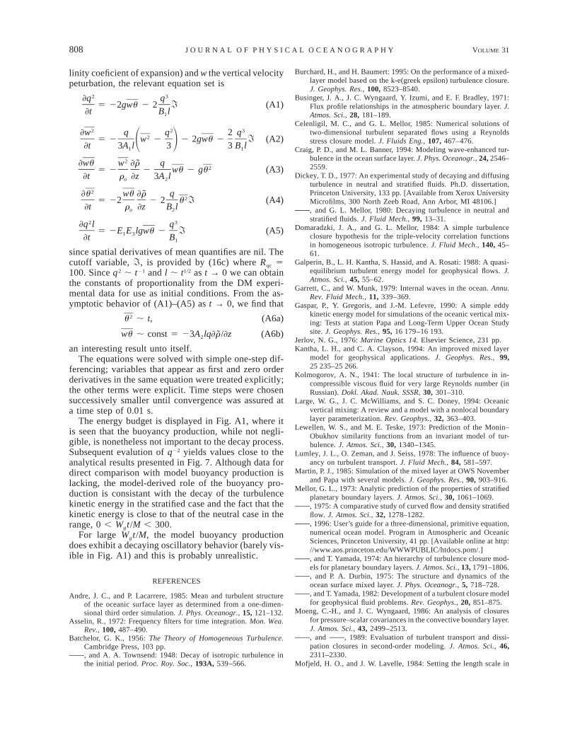
linity coeficient of expansion) and w the vertical velocitypeturbation, the relevant equation set is

2 3]q q5 22gwu 2 2 I (A1)

]t B l1

2 2 3]w q q 2 q25 2 w 2 2 2gwu 2 I (A2)1 2]t 3A l 3 3 B l1 1

2]wu w ]r q25 2 2 wu 2 gu (A3)

]t r ]z 3A lo 2

2]u wu ]r q25 22 2 2 u I (A4)

]t r ]z B lo 2

2 3]q l q5 2E E lgwu 2 I (A5)1 3]t B1

since spatial derivatives of mean quantifies are nil. Thecutoff variable, I, is provided by (16c) where Rqc 5100. Since q2 ; t21 and l ; t1/2 as t → 0 we can obtainthe constants of proportionality from the DM experi-mental data for use as initial conditions. From the as-ymptotic behavior of (A1)–(A5) as t → 0, we find that

2u ; t, (A6a)

wu ; const 5 23A lq]r /]z (A6b)2

an interesting result unto itself.The equations were solved with simple one-step dif-

ferencing; variables that appear as first and zero orderderivatives in the same equation were treated explicitly;the other terms were explicit. Time steps were chosensuccessively smaller until convergence was assured ata time step of 0.01 s.

The energy budget is displayed in Fig. A1, where itis seen that the buoyancy production, while not negli-gible, is nonetheless not important to the decay process.Subsequent evalution of q22 yields values close to theanalytical results presented in Fig. 7. Although data fordirect comparison with model buoyancy production islacking, the model-derived role of the buoyancy pro-duction is consistant with the decay of the turbulencekinetic energy in the stratified case and the fact that thekinetic energy is close to that of the neutral case in therange, 0 , Wgt/M , 300.

For large Wgt/M, the model buoyancy productiondoes exhibit a decaying oscillatory behavior (barely vis-ible in Fig. A1) and this is probably unrealistic.

REFERENCES

Andre, J. C., and P. Lacarrere, 1985: Mean and turbulent structureof the oceanic surface layer as determined from a one-dimen-sional third order simulation. J. Phys. Oceanogr., 15, 121–132.

Asselin, R., 1972: Frequency filters for time integration. Mon. Wea.Rev., 100, 487–490.

Batchelor, G. K., 1956: The Theory of Homogeneous Turbulence.Cambridge Press, 103 pp., and A. A. Townsend: 1948: Decay of isotropic turbulence inthe initial period. Proc. Roy. Soc., 193A, 539–566.

Burchard, H., and H. Baumert: 1995: On the performance of a mixed-layer model based on the k-e(greek epsilon) turbulence closure.J. Geophys. Res., 100, 8523–8540.

Businger, J. A., J. C. Wyngaard, Y. Izumi, and E. F. Bradley, 1971:Flux profile relationships in the atmospheric boundary layer. J.Atmos. Sci., 28, 181–189.

Celenligil, M. C., and G. L. Mellor, 1985: Numerical solutions oftwo-dimensional turbulent separated flows using a Reynoldsstress closure model. J. Fluids Eng., 107, 467–476.

Craig, P. D., and M. L. Banner, 1994: Modeling wave-enhanced tur-bulence in the ocean surface layer. J. Phys. Oceanogr., 24, 2546–2559.

Dickey, T. D., 1977: An experimental study of decaying and diffusingturbulence in neutral and stratified fluids. Ph.D. dissertation,Princeton University, 133 pp. [Available from Xerox UniversityMicrofilms, 300 North Zeeb Road, Ann Arbor, MI 48106.], and G. L. Mellor, 1980: Decaying turbulence in neutral andstratified fluids. J. Fluid Mech., 99, 13–31.

Domaradzki, J. A., and G. L. Mellor, 1984: A simple turbulenceclosure hypothesis for the triple-velocity correlation functionsin homogeneous isotropic turbulence. J. Fluid Mech., 140, 45–61.

Galperin, B., L. H. Kantha, S. Hassid, and A. Rosati: 1988: A quasi-equilibrium turbulent energy model for geophysical flows. J.Atmos. Sci., 45, 55–62.

Garrett, C., and W. Munk, 1979: Internal waves in the ocean. Annu.Rev. Fluid Mech., 11, 339–369.

Gaspar, P., Y. Gregoris, and J.-M. Lefevre, 1990: A simple eddykinetic energy model for simulations of the oceanic vertical mix-ing: Tests at station Papa and Long-Term Upper Ocean Studysite. J. Geophys. Res., 95, 16 179–16 193.

Jerlov, N. G., 1976: Marine Optics 14. Elsevier Science, 231 pp.Kantha, L. H., and C. A. Clayson, 1994: An improved mixed layer

model for geophysical applications. J. Geophys. Res., 99,25 235–25 266.

Kolmogorov, A. N., 1941: The local structure of turbulence in in-compressible viscous fluid for very large Reynolds number (inRussian). Dokl. Akad. Nauk. SSSR, 30, 301–310.

Large, W. G., J. C. McWilliams, and S. C. Doney, 1994: Oceanicvertical mixing: A review and a model with a nonlocal boundarylayer parameterization. Rev. Geophys., 32, 363–403.

Lewellen, W. S., and M. E. Teske, 1973: Prediction of the Monin–Obukhov similarity functions from an invariant model of tur-bulence. J. Atmos. Sci., 30, 1340–1345.

Lumley, J. L., O. Zeman, and J. Seiss, 1978: The influence of buoy-ancy on turbulent transport. J. Fluid Mech., 84, 581–597.

Martin, P. J., 1985: Simulation of the mixed layer at OWS Novemberand Papa with several models. J. Geophys. Res., 90, 903–916.

Mellor, G. L., 1973: Analytic prediction of the properties of stratifiedplanetary boundary layers. J. Atmos. Sci., 30, 1061–1069., 1975: A comparative study of curved flow and density stratifiedflow. J. Atmos. Sci., 32, 1278–1282., 1996: User’s guide for a three-dimensional, primitive equation,numerical ocean model. Program in Atmospheric and OceanicSciences, Princeton University, 41 pp. [Available online at http://www.aos.princeton.edu/WWWPUBLIC/htdocs.pom/.], and T. Yamada, 1974: An hierarchy of turbulence closure mod-els for planetary boundary layers. J. Atmos. Sci., 13, 1791–1806., and P. A. Durbin, 1975: The structure and dynamics of theocean surface mixed layer. J. Phys. Oceanogr., 5, 718–728., and T. Yamada, 1982: Development of a turbulent closure modelfor geophysical fluid problems. Rev. Geophys., 20, 851–875.

Moeng, C.-H., and J. C. Wyngaard, 1986: An analysis of closuresfor pressure–scalar covariances in the convective boundary layer.J. Atmos. Sci., 43, 2499–2513., and , 1989: Evaluation of turbulent transport and dissi-pation closures in second-order modeling. J. Atmos. Sci., 46,2311–2330.

Mofjeld, H. O., and J. W. Lavelle, 1984: Setting the length scale in


a second order closure model of the unstratified bottom boundarylayer. J. Phys. Oceanogr., 14, 833–839.

Paulson, C. A., and J. J. Simpson, 1977: Irradiance measurements inthe upper ocean. J. Phys. Oceanogr., 7, 952–956.

Pollard, R. T., 1970: On the generation of inertial waves in the ocean.Deep-Sea Res., 17, 795–812., and R. C. Millard, 1970: Comparison between observed andsimulated wind-generated inertial oscillations. Deep-Sea Res.,17, 813–821.

Price, J. F., R. A. Weller, C. M. Bowers, and M. G. Briscoe, 1987:Diurnal response of sea surface temperature observed at theLong-Term Upper Ocean Study (348N, 708W) in the SargassoSea. J. Geophys. Res., 92, 14 480–14 490.

Rodi, W., 1987: Examples of calculation methods for flow and mixingin stratified flows. J. Geophys. Res., 92, 5305–5328.

Rotta, J. C., 1951a: Statistische Theorie nichthomogener Turbulenz.Z. Phys., 129, 547–572.

, 1951b: Statistische Theorie nichthomogener Turbulenz. Z.Phys., 131, 51–77.

Stacey, M. W., and S. Pond, 1997: On the Mellor–Yamada turbulenceclosure scheme: The surface boundary conditions for q2. J. Phys.Oceanogr., 27, 2081–2086.

Stramma, L. P., P. Cornillon, R. A. Weller, J. F. Price, and M. G. Briscoe,1986: Large diurnal sea surface temperature variability: Satellite andin situ measurements. J. Phys. Oceanogr., 16, 827–837.

Sun, W.-Y., and Y. Ogura, 1980: Modeling the evolution of theconvective planetary boundary layer. J. Atmos. Sci., 37, 1558–1572.

Taylor, G. I., 1921: Diffusion by continuous movement. Proc. LondonMath. Soc., 20, 196–211.

Therry, G., and P. Lacarrere, 1986: Improving the eddy-kinetic energymodel for boundary layer description. Bound.-Layer Meteor.,37, 129–148.

Yamada, T., 1983: Simulations of nocturnal drainage flows by a q221turbulence closure model. J. Atmos. Sci., 40, 90–106.

one-dimensional, ocean surface layer modeling - geophysical

Documents