one-factor repeated measures anova - the home page for astro…andykarp/graduate_statistics... ·...

Chapter 10 One-Factor Repeated Measures ANOVA

Page Introduction to Repeated Measures

1. Types of repeated measures designs 10-2 2. Advantages and disadvantages 10-5 3. The paired t-test 10-5 4. Analyzing paired data 10-15

One-Factor Repeated Measures ANOVA

5. An initial example 10-18 6. Structural model, SS partitioning, and the ANOVA table 10-19 7. Repeated measures as a randomized block design 10-26 8. Assumptions 10-27 9. Contrasts 10-39 10. Planned and post-hoc tests 10-46 11. Effect sizes 10-48 12. A final example 10-51

10-1 © 2011 A. Karpinski

Repeated Measures ANOVA One-Factor Repeated Measures

1. Types of repeated measures designs

i. Each participant/unit is observed in a different treatment conditions

o Example: Testing over the counter headache remedies

Each participant is given four over-the-counter headache medicines: • Tylenol (Acetaminophen) • Advil (Ibuprofen) • Goody’s Headache Powder (??) • An herbal remedy (Ginkgo)

Over-The-Counter Headache Remedies

Tylenol Advil Goody’s Ginkgo

Spee

d of

Hea

dach

e R

elie

f

o If each participant takes the treatments in random order, then this design can be treated as a randomized block design with participant as the block

Treatment Order 1 2 3 4

Block 1 A T GI GO

2 GO A GI T

3 T GO A GI

4 GI T GO A

5 GO A GI T


ii. Profile analysis

Scores on a different tests are compared for each participant

o Each participant completes several different scales, and the profile of responses to those scores is examined.

o Example: Perceptions of a loving relationship

Single male and female participants complete three scales, each designed to measure a different aspect of Sternberg’s (1988) love triangle: • Intimacy • Passion • Commitment Participants rate the importance of each component for a long-term relationship.

Perceptions of Long-Term Love

2

4

6

8

10

Intimacy Passion Commitment

MalesFemales

o This example has a repeated measures factor and a between-subjects factor.

o For a profile analysis, it is highly desirable that each questionnaire is

scaled similarly (with the same mean and standard deviation) so that the profile comparison is meaningful.

o A common use of profile analysis is to examine the profile of MMPI

subscale scores.


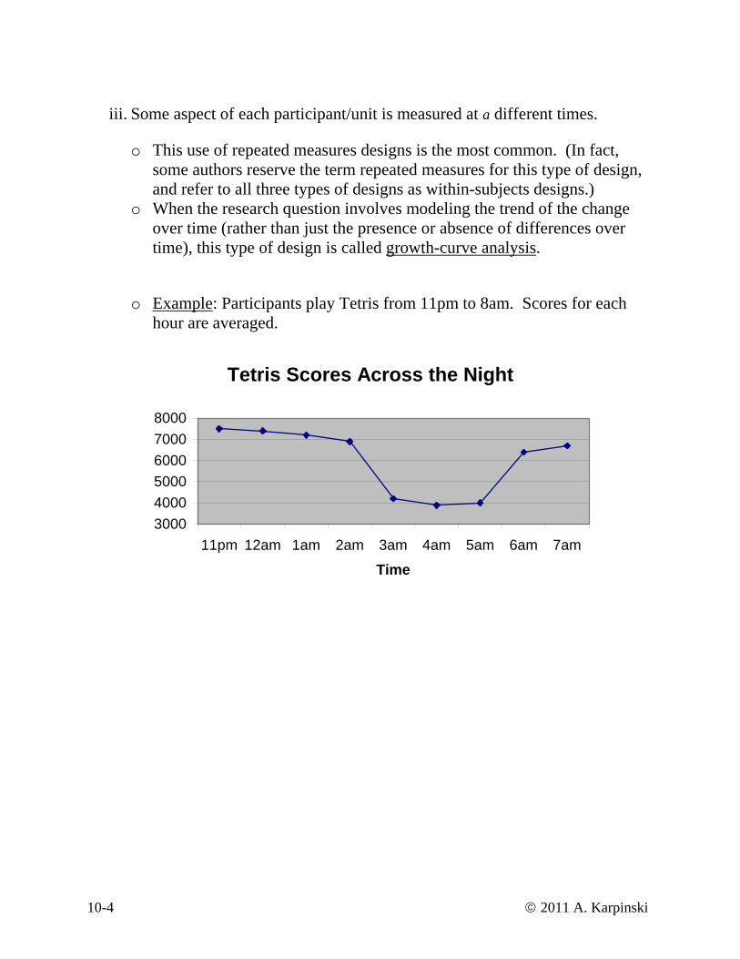
iii. Some aspect of each participant/unit is measured at a different times.

o This use of repeated measures designs is the most common. (In fact,

some authors reserve the term repeated measures for this type of design, and refer to all three types of designs as within-subjects designs.)

o When the research question involves modeling the trend of the change over time (rather than just the presence or absence of differences over time), this type of design is called growth-curve analysis.

o Example: Participants play Tetris from 11pm to 8am. Scores for each hour are averaged.

Tetris Scores Across the Night

300040005000600070008000

11pm 12am 1am 2am 3am 4am 5am 6am 7am

Time


2. Advantages and Disadvantages of Repeated Measures Designs

• Advantages o Each participant serves as his or her own control. (You achieve perfect

equivalence of all groups / perfect blocking) o Fewer participants are needed for a repeated measures design to achieve

the same power as a between-subjects design. (Individual differences in the DV are measured and removed from the error term.)

o The most powerful designs for examining change and/or trends

• Disadvantages

o Practice effects

o Differential carry-over effects

o Demand characteristics 3. The Paired t-test

• The simplest example of a repeated measures design is a paired t-test. o Each subject is measured twice (time 1 and time 2) on the same variable o Or each pair of matched participants are assigned to one of two treatment

levels

• The analysis of a paired t-test is exactly equivalent to a one sample t-test conducted on the difference of the time 1 and time 2 scores (or on the difference of the matched pair)


• Understanding the paired t-test o Recall that for an independent samples t-test, we used the following

formula (see p. 2-39)

21

21

11

nns

XX

estimateoferrorstdestimatet

pooled

obs

+

−=

=

where

)2()1()1(

)2(

21

222

211

21

21

−+−+−

=

−++

=

nnsnsn

s

nnSSSS

s

pooled

pooled

df = n1 + n2 - 2

o For a paired t-test, we will conduct the analysis on the difference of the time 1 and time 2 observations.

Subject Pre-test Post-Test Difference 1 6 9 -3 2 4 6 -2 3 6 5 1 4 7 10 -3 5 4 10 -6 6 5 8 -3 7 5 7 -2 8 12 10 2 9 6 6 0 10 1 5 -4 Average 5.4 7.4 -2

ns

D

estimateoferrorstdestimatet

D

obs

1

=

=

where 1−

=nSS

s DD

df = n – 1


o First, let’s see how this analysis would differ if we “forgot” we had a repeated measures design, and treated it as an independent-samples design

• We treat each of the 20 observations as independent observations • To analyze in SPSS, we need 20 lines of data, ostensibly one line for

each participant

T-TEST GROUPS=group(1 2) /VARIABLES=dv.

Independent Samples Test

-1.819 18 .086 -2.0000 1.09949 -4.30995 .30995Equal variancesassumed

DVt df Sig. (2-tailed)

MeanDifference

Std. ErrorDifference Lower Upper

95% ConfidenceInterval of the

Difference

t-test for Equality of Means

t(18) = -1.82, p = .086

• But this analysis is erroneous! We do not have 20 independent data points (18 df).


o Now, let’s conduct the proper paired t-test in SPSS: • We properly treat the data as 10 pairs of observations. • To conduct this analysis in SPSS, we need to enter our data differently

than for a between-subjects design. The data from each participant are entered on one line

T-TEST PAIRS time1 time2.

Paired Samples Correlations

10 .546 .102TIME1 & TIME2Pair 1N Correlation Sig.

Paired Samples Test

-2.0000 2.40370 .76012 -3.7195 -.2805 -2.631 9 .027TIME1 - TIME2Pair 1Mean Std. Deviation

Std. ErrorMean Lower Upper


Difference

Paired Differences

t df Sig. (2-tailed)

t(9) = -2.63, p = .027


o We could also obtain the same result by conducting a one-sample t-test

on the difference between time 1 and time 2: COMPUTE diff = time1 – time2. T-TEST /TESTVAL=0 /VARIABLES=diff.

One-Sample Test

-2.631 9 .027 -2.0000 -3.7195 -.2805DIFFt df Sig. (2-tailed)

MeanDifference Lower Upper


Difference

Test Value = 0

• Both analyses give the identical results: t(9) = -2.63, p = .027

o A comparison of the differences of the two analyses:

Independent Groups

Repeated Measures

Mean Difference -2.00 -2.00 Standard Error 1.10 0.76 t-value -1.82 -2.63 p-value .086 .027

• The mean difference is the same • Importantly, the standard error is smaller in the repeated measures

case. The smaller standard error results in a larger t-value and a smaller p-value


• The greater the correlation between the time 1 and the time 2 observations, the greater the advantage gained by using a repeated measures design.

Recall that the variance of the difference between two variables is given by the following formula (see p 2-38)

Var(X1 − X2 ) = Var(X1) +Var(X2 ) −2Cov(X1,X2 ) (Formula 8-1) The covariance of and is a measure of the association between the two variables. If we standardize the covariance (so that it ranges from –1 to +1), we call it the correlation between and

1X 2X

1X 2X

ρ12 =Cov(X1,X2 )

Var(X1)*Var(X2 )

If we rearrange the terms and substitute into (Formula 8-1), we obtain a formula for the variance of the difference scores:

Cov(X1, X2) = ρ12 * Var(X1) * Var(X2)

Var(X1 − X2 ) = Var(X1) +Var(X2 ) −2ρ12 * Var(X1) * Var(X2 )

σD2 = σX1

2 + σX 2

2 − 2ρ12σ X1σX 2

And finally, we can obtain the standard error of the difference scores:

In the population: σD 2 =

σ X1

2

n+

σX2

2

n−

2ρ12σ X1σ X2

n

σD =1n

σ X1

2 + σX2

2 −2ρ12σ X1σX 2( )

In the sample : sD =s1

2

n+

s22

n−

2r12s1 s2

n

Ds =1n

s12 + s2

2 − 2r12s1 s2( )


⇒ If 0

21=XXr , then the variance of the difference scores is equal to

σX2 +

1σX 2

2 ⇒ As

21XXr becomes greater, then the variance of the difference scores becomes smaller than σX1

2 + σX 2

2

So the greater the correlation between time 1 and time 2 scores, the greater the advantage of using a paired t-test.

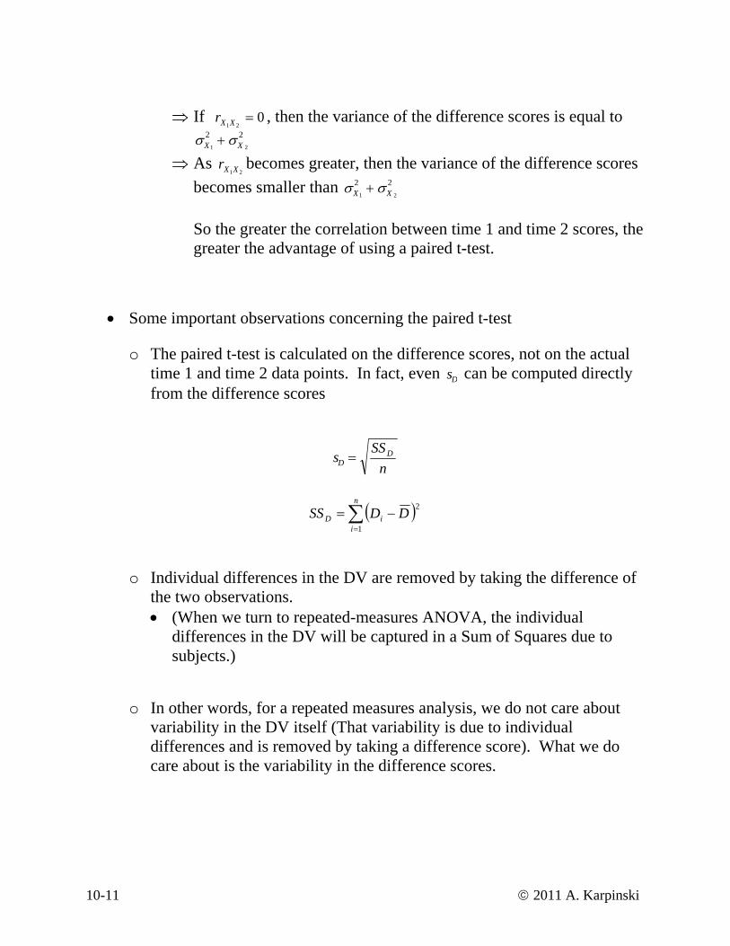
• Some important observations concerning the paired t-test

o The paired t-test is calculated on the difference scores, not on the actual time 1 and time 2 data points. In fact, even sD can be computed directly from the difference scores

sD nSSD=

( )∑=

−=n

iiD DDSS

1

2

o Individual differences in the DV are removed by taking the difference of the two observations. • (When we turn to repeated-measures ANOVA, the individual

differences in the DV will be captured in a Sum of Squares due to subjects.)

o In other words, for a repeated measures analysis, we do not care about variability in the DV itself (That variability is due to individual differences and is removed by taking a difference score). What we do care about is the variability in the difference scores.


o An example might help clarify this issue. Suppose we add 10 to the pre- and post-test scores of the first five participants

Original Data Modified Data Participant Pre-

test Post-Test

Difference Pre-test

Post-Test

Difference

1 6 9 -3 16 19 -3 2 4 6 -2 14 16 -2 3 6 5 -1 16 15 -1 4 7 10 -3 17 20 -3 5 4 10 -6 14 20 -6 6 5 8 -3 5 8 -3 7 5 7 -2 5 7 -2 8 12 10 2 12 10 2 9 6 6 0 6 6 0 10 1 5 -4 1 5 -4 Average 5.4 7.4 -2 10.4 12.4 -2

• We have increased the amount of individual differences in the pre- and post-test data, but we have not changed the difference scores.

• As a result, a between-subject analysis of this data is greatly affected

by the addition of extra noise to the data, but a within-subject analysis of this data is unchanged.

Original Data Modified Data Between-Subjects t(18) = -1.82 t(18) = -0.76 p = .086 p = .459 SE = 1.10 SE = 2.64 Within-Subjects t(9) = -2.63 t(9) = -2.63 p = .027 p = .027 SE = 0.760 SE = 0.760


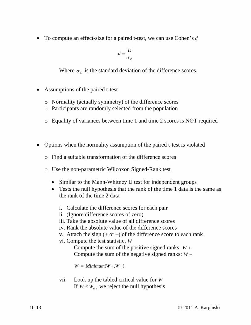
• To compute an effect-size for a paired t-test, we can use Cohen’s d

D

Ddσ

=

Where Dσ is the standard deviation of the difference scores.

• Assumptions of the paired t-test

o Normality (actually symmetry) of the difference scores o Participants are randomly selected from the population

o Equality of variances between time 1 and time 2 scores is NOT required

• Options when the normality assumption of the paired t-test is violated

o Find a suitable transformation of the difference scores

o Use the non-parametric Wilcoxon Signed-Rank test

• Similar to the Mann-Whitney U test for independent groups • Tests the null hypothesis that the rank of the time 1 data is the same as

the rank of the time 2 data

i. Calculate the difference scores for each pair ii. (Ignore difference scores of zero) iii. Take the absolute value of all difference scores iv. Rank the absolute value of the difference scores v. Attach the sign (+ or –) of the difference score to each rank vi. Compute the test statistic, W

Compute the sum of the positive signed ranks: +WCompute the sum of the negative signed ranks: −W W = ),( −+ WWMinimum

vii. Look up the tabled critical value for W If we reject the null hypothesis critWW ≤


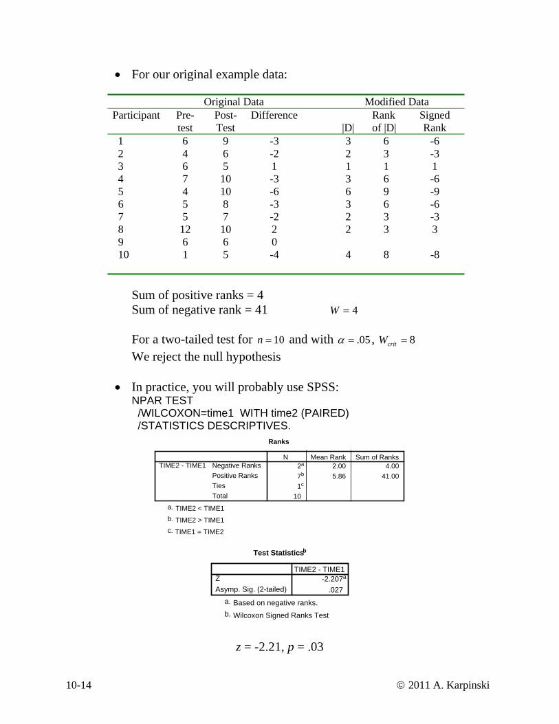
• For our original example data:

Original Data Modified Data Participant Pre-

test Post-Test

Difference |D|

Rank of |D|

Signed Rank

1 6 9 -3 3 6 -6 2 4 6 -2 2 3 -3 3 6 5 1 1 1 1 4 7 10 -3 3 6 -6 5 4 10 -6 6 9 -9 6 5 8 -3 3 6 -6 7 5 7 -2 2 3 -3 8 12 10 2 2 3 3 9 6 6 0 10 1 5 -4 4 8 -8

Sum of positive ranks = 4 Sum of negative rank = 41 4=W

For a two-tailed test for 10=n and with 05.=α , 8=critWWe reject the null hypothesis

• In practice, you will probably use SPSS:

NPAR TEST /WILCOXON=time1 WITH time2 (PAIRED) /STATISTICS DESCRIPTIVES.

Ranks

2a 2.00 4.007b 5.86 41.001c

10

Negative RanksPositive RanksTiesTotal

TIME2 - TIME1N Mean Rank Sum of Ranks

TIME2 < TIME1a.

TIME2 > TIME1b.

TIME1 = TIME2c.

Test Statisticsb

-2.207a

.027ZAsymp. Sig. (2-tailed)

TIME2 - TIME1

Based on negative ranks.a.

Wilcoxon Signed Ranks Testb.

z = -2.21, p = .03


4. Analyzing paired data: An example

• To investigate the effectiveness of a new method of mathematical instruction, 30 middle-school students were matched (in pairs) on their mathematical ability. Within the pair, students were randomly assigned to receive the traditional mathematics instruction or to receive a new method of instruction. At the end of the study, all participants took the math component of the California Achievement Test (CAT). The following data were obtained:

Method of Instruction Pair Traditional New

1 78 74 2 55 45 3 95 88 4 57 65 5 60 64 6 80 75 7 50 41 8 83 68 9 90 80 10 70 64 11 50 43 12 80 82 13 48 55 14 65 57 15 85 75

• First, let’s check assumptions necessary for statistical testing

o The participants who received the old and new methods of instruction are not independent of each other (they are matched on ability), so an independent samples t-test is not appropriate. We can use a paired t-test.

o The assumptions of the pair t-test are:

• Participants are randomly selected from the population • Normality (actually symmetry) of the difference scores

Compute diff = old - new. EXAMINE VARIABLES=diff /PLOT BOXPLOT STEMLEAF NPPLOT.


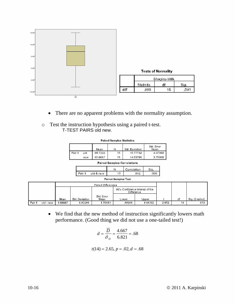
• There are no apparent problems with the normality assumption.

o Test the instruction hypothesis using a paired t-test. T-TEST PAIRS old new.

• We find that the new method of instruction significantly lowers math performance. (Good thing we did not use a one-tailed test!)

68.821.6667.4

ˆ===

D

Ddσ

68.,02.,65.2)14( === dpt


o We could have also analyzed these data as a randomized block design • (Be careful! The data must be entered differently in SPSS for this

analysis.) UNIANOVA cat BY instruct block /DESIGN = instruct block.

• The test for the method instruction is identical to the paired t-test. 02.,02.7)14,1( == pF

• In this case, we also obtain a direct test for the effect of the matching

on the math scores. 01.,79.18)14,14( <= pF

o If we are concerned about the normality/symmetry of the difference

scores, then we can turn to a non-parametric test. NPAR TEST /WILCOXON=old WITH new (PAIRED) /STAT DESC.

02.,28.2 =−= pz


One-Factor Repeated Measures ANOVA

• If we observe participants at more than two time-points, then we need to conduct a repeated measures ANOVA

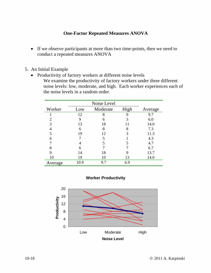
5. An Initial Example

• Productivity of factory workers at different noise levels We examine the productivity of factory workers under three different noise levels: low, moderate, and high. Each worker experiences each of the noise levels in a random order.

Noise Level Worker Low Moderate High Average 1 12 8 9 9.7 2 9 6 3 6.0 3 13 18 11 14.0 4 6 8 8 7.3 5 19 12 3 11.3 6 7 5 1 4.3 7 4 5 5 4.7 8 6 7 7 6.7 9 14 18 9 13.7 10 19 10 13 14.0 Average 10.9 9.7 6.9

Worker Productivity

0

4

8

12

16

20

Low Moderate High

Noise Level

Prod

uctiv

ity


6. Structural model, SS partitioning, and the ANOVA table

• What we would like to do is to decompose the variability in the DV into o Variability due to individual differences in the participants

A random effect o Variability due to the factor (low, moderate, or high)

A fixed effect

o The effect of participants is always a random effect o We will only consider situations where the factor is a fixed effect

• The structural model for a one-way within-subjects design

ijijijY επαμ σ +++= or

Yij = μ + α j + πσ i + απ( )σ ij

μ = Grand population mean

..ˆ Y=μ

jα = The treatment/time effect: The effect of being in level j of the factor Or the effect of being at time j ∑ = 0jα

...ˆ YY jj −=α

iσπ = The participant effect: The random effect due to participant i πσ i ~ N(0,σ π )

εij or απ( )σ ij

= The unexplained error associated with ijY

....ˆ YYYY jiijij +−−=ε

o Note that with only one observation on each participant at each level of the factor (or at each time), we can not estimate the participant by factor/time interaction

o This structural model is just like the model for a randomized block

design, with participants as a random blocking effect


• Now, we can identify SS due to the factor of interest, and divide the error

term into a SS due to individual differences in the participants, and a SS residual (everything we still can not explain)

SS Total (SS Corrected Total)

SS Within df = N-a

SS Factor df=(a-1)

• Sums of squares decomposition and ANOVA table for a repeated measures design:

Source SS df MS E(MS) F

Treatment/Time SSA a-1 MSA

1

22

−+ ∑

an jα

σ ε MSEMSA

Subjects SS(Subject) n-1 MS(Sub) 22πε σσ n+

MSESubMS )(

Error SSError (a-1)(n-1) MSE 2εσ

Total SST N-1

SS Subjects df = n-1

SS Residual Df = (a-1)(n-1)

= N – a – n + 1

SS A df=(a-1)


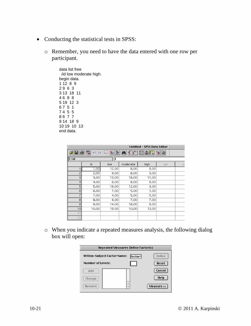
• Conducting the statistical tests in SPSS:

o Remember, you need to have the data entered with one row per

participant.

data list free /id low moderate high. begin data. 1 12 8 9 2 9 6 3 3 13 18 11 4 6 8 8 5 19 12 3 6 7 5 1 7 4 5 5 8 6 7 7 9 14 18 9 10 19 10 13 end data.

o When you indicate a repeated measures analysis, the following dialog box will open:


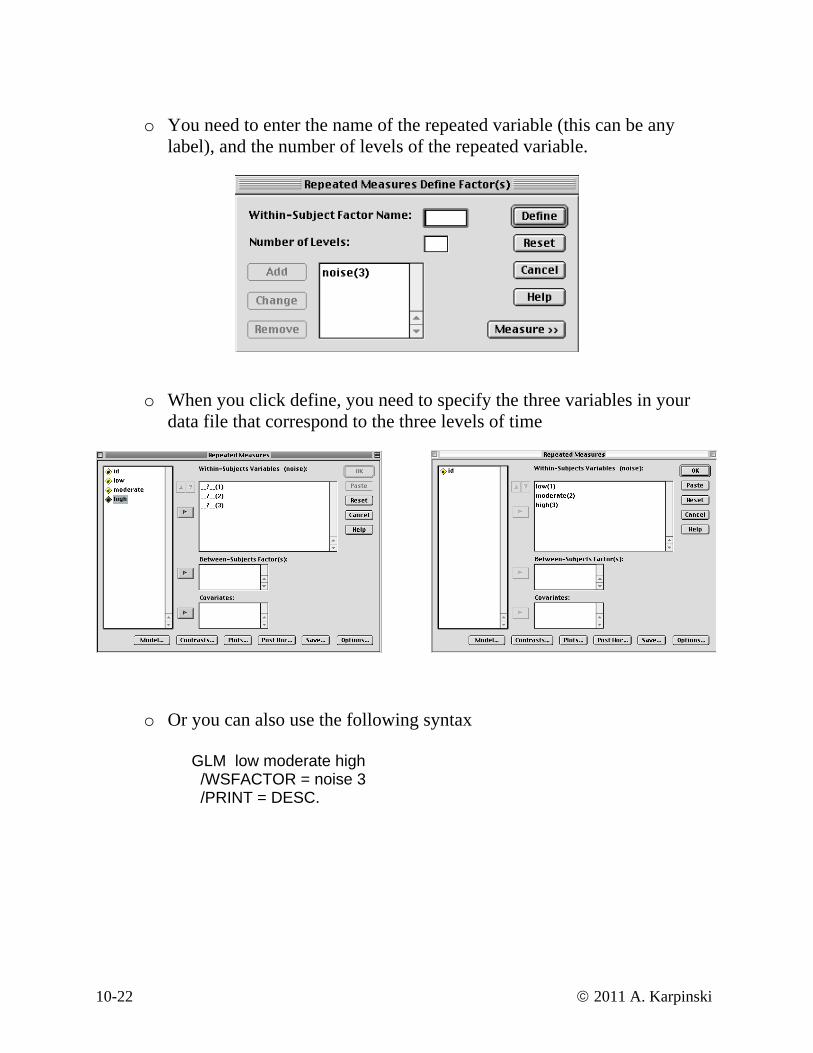
o You need to enter the name of the repeated variable (this can be any

label), and the number of levels of the repeated variable.

o When you click define, you need to specify the three variables in your

data file that correspond to the three levels of time

o Or you can also use the following syntax

GLM low moderate high /WSFACTOR = noise 3 /PRINT = DESC.


o Here is the (unedited) output file: General Lin

ear Model

Within-Subjects Factors

Measure: MEASURE_1

LOWMODERATEHIGH

NOISE123

DependentVariable

Reperepeated m

ats the levels of the easure variable

that you entered

Descriptive Statistics

10.9000 5.38413 109.7000 4.87739 106.9000 3.84274 10

LOWMODERATEHIGH

Mean Std. Deviation N

Produced by the /PRINT = DESC command

Multivariate Testsb

.422 2.918a 2.000 8.000 .112

.578 2.918a 2.000 8.000 .112

.730 2.918a 2.000 8.000 .112

.730 2.918a 2.000 8.000 .112

Pillai's TraceWilks' LambdaHotelling's TraceRoy's Largest Root

EffectNOISE

Value F Hypothesis df Error df Sig.

Exact statistica.

Design: Intercept Within Subjects Design: NOISE

b.

These are multivariate tests of repeated measures. We will ignore these tests.

Mauchly's Test of Sphericityb

Measure: MEASURE_1

.945 .456 2 .796 .947 1.000 .500Within Subjects EffectNOISE

Mauchly's WApprox.

Chi-Square df Sig.Greenhouse-Geisser Huynh-Feldt Lower-bound

Epsilona

Tests the null hypothesis that the error covariance matrix of the orthonormalized transformed dependent variables isproportional to an identity matrix.

May be used to adjust the degrees of freedom for the averaged tests of significance. Corrected tests are displayed in theTests of Within-Subjects Effects table.

a.

Design: Intercept Within Subjects Design: NOISE

b.

This box will help us test one of the key assumptions for repeated-measures


Tests of Within-Subjects Effects

Measure: MEASURE_1

84.267 2 42.133 3.747 .04484.267 1.895 44.469 3.747 .04784.267 2.000 42.133 3.747 .04484.267 1.000 84.267 3.747 .085

202.400 18 11.244202.400 17.054 11.868202.400 18.000 11.244202.400 9.000 22.489

Sphericity AssumedGreenhouse-GeisserHuynh-FeldtLower-boundSphericity AssumedGreenhouse-GeisserHuynh-FeldtLower-bound

SourceNOISE

Error(NOISE)

Type III Sumof Squares df Mean Square F Sig.

The test listed under “Sphericity Assumed” is the omnibus repeated measures test of the time factor

Tests of Within-Subjects Contrasts

Measure: MEASURE_1

80.000 1 80.000 5.806 .0394.267 1 4.267 .490 .502

124.000 9 13.77878.400 9 8.711

NOISELinearQuadraticLinearQuadratic

SourceNOISE

Error(NOISE)


These are contrasts specified by the command “Polynomial” which are performed on the time variable

Tests of Between-Subjects Effects

Measure: MEASURE_1Transformed Variable: Average

2520.833 1 2520.833 55.949 .000405.500 9 45.056

SourceInterceptError


These are tests on the between-subjects factors in the design (in this case there are none)


• Let’s fill in a standard ANOVA table for a repeated measures design, using the SPSS output labeled “Tests of Within-Subjects Effects”

Source SS df MS F p

Noise 84.267 2 42.133 3.747 .044 Subjects Error (Noise) 202.4 18 11.244 Total

o SPSS does not print a test for the random effect of subject. It also does

not print SST. o We showed previously that for a one-factor repeated measures design,

the error term for Subjects is the same as the error term for Noise. If we had the SS (Subjects), we could construct the test ourselves.

o In general, however, we are not interested in the test of the effect of individual differences due to subjects.

o The noise effect compares the marginal noise means, using an appropriate error term [MSE(noise)]

Noise Level

Low Moderate High 10.9 9.7 6.9

H0 : μ.1 = μ.2 = μ.3H0 :α1 = α2 = α3 = 0

F(2,18) = 3.75, p = .04

We conclude that productivity is not the same at all three noise levels. We need to conduct follow-up tests to determine exactly how these means differ.


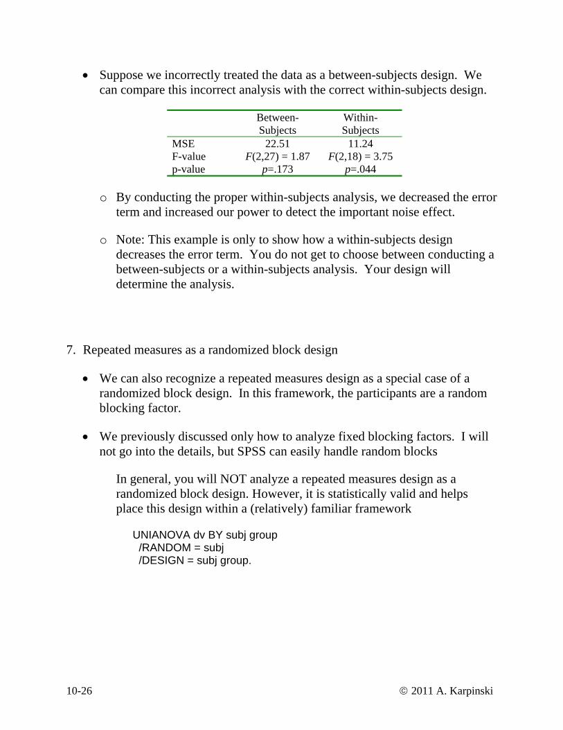
• Suppose we incorrectly treated the data as a between-subjects design. We

Subjects Subjects

can compare this incorrect analysis with the correct within-subjects design.

Between- Within-

MSE 22.51 11.24 F-value ,27) = 1. F(2,18) = 3.75 p p=.173 p=.

F(2 87 -value 044

nduct proper thin-s

term and increased our power to detect the important noise effect.

rror term. You do not get to choose between conducting a

. Repeated measures as a randomized block design

es design as a special case of a randomized block design. In this framework, the participants are a random blocking factor.

• We previously discussed only how to analyze fixed blocking factors. I will

not go into the details, but SPSS can easily handle random blocks

In general, you will NOT analyze a repeated measures design as a randomized block design. However, it is statistically valid and helps place this tively) familiar framework

o By co ing the wi ubjects analysis, we decreased the error

o Note: This example is only to show how a within-subjects design

decreases the ebetween-subjects or a within-subjects analysis. Your design will determine the analysis.

7

• We can also recognize a repeated measur

design within a (rela

UNIANOVA dv BY subj group /RANDOM = subj /DESIGN = subj group.


Tests of Between-Subjects Effects

Dependent Variable: DV

2520.833 1 2520.833 55.949 .000405.500 9 45.056a

405.500 9 45.056 4.007 .006202.400 18 11.244b

84.267 2 42.133 3.747 .044202.400 18 11.244b

SourceH hesisypotError

Intercept

HypothesisError

SUBJ

HypothesisError

NOISE


MS(SUBJ)a.

MS(Error)b.

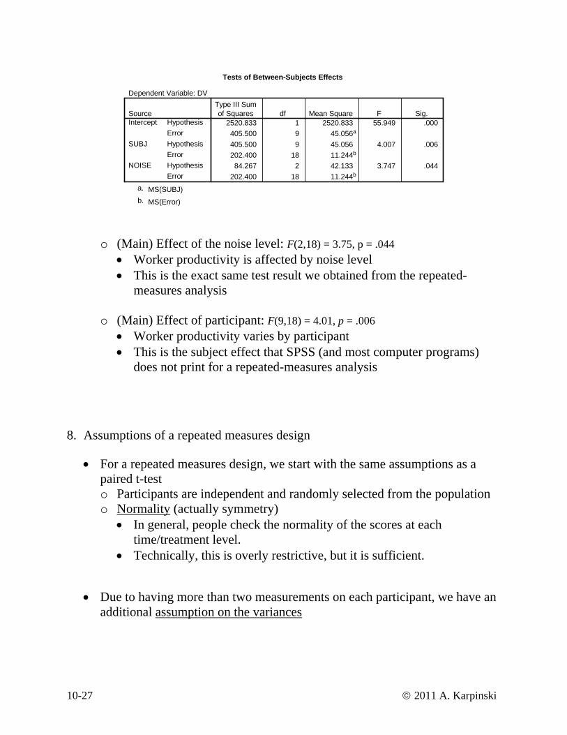
o (Main) Effect of the noise level: F(2,18) = 3.75, p = .044 • Worker productivity is affected by noise level • This is the exact same test result we obtained from the repeated

measures analysis -

o (Main) Effect of participant: F(9,18) = 4.01, p = .006 • Worker productivity varies by participant

ost computer programs) does not print for a repeated-measures analysis

paio on o

• This is the subject effect that SPSS (and m

8. Assumptions of a repeated measures design

• For a repeated measures design, we start with the same assumptions as a red t-test Participants are independent and randomly selected from the populatiNormality (actually symmetry) • In general, people check the normality of the scores at each

• ly restrictive, but it is sufficient.

• Due to having more than two measurements on each participant, we have an additional assumption on the variances

time/treatment level. Technically, this is over


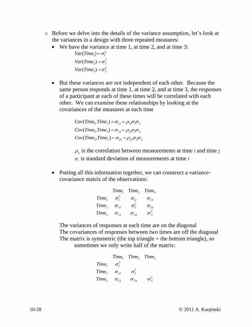
o Before we delve into the details of the variance assumption, let’s look at the variances in a design with three repeated measures: • We have the variance at time 1, at time 2, and at time 3:

Var(Time1) = σ12

Var(Time2) =σ 22

Var(Time3) =σ 32

• But these variances are not independent of each other. Because the

same person responds at time 1, at time 2, and at time 3, the responses of a participant at each of these times will be correlated with each other. We can examine these relationships by looking at the

covariances of the measures at each time

Cov(Time1,Time2) =σ12 = ρ12σ1σ 2

Cov(Time1,Time3) =σ13 = ρ13σ1σ 3

Cov(Time = σ = ρ σ σ

2,Time3 ) 23 23 2 3

is the correlation between measurements at time i and time j ρij

σ i is standard deviation of measurements at time i

• Putting all this information together, we can construct a variance-covariance matrix of the observations:

Time1 Time2

2 σTime3

Time1 σ1 12 σ13

Time3 σ13 σ 23 σ 32

Time2 σ12 σ2 σ23

2

e are on the diagonal diagonal

ric (the top triangle = the bottom triangle), so

The variances of responses at each timThe covariances of responses between two times are off the The matrix is symmet

sometimes we only write half of the matrix:

Time1 Time2 Time3

Time3 σ13 σ 23 σ 32

Time1 σ12

Time2 σ12 σ2

2


o Now, we can examine the assumption of compound symmetry. Compound symmetry specifies a specific structure for the

• All of the variances are equal:

variance/covariance matrix where:

σ 2 σ12 =σ 2

2 = σ32

• All of the covariances are equal: σ12 =σ13 = σ23 σc

• If we divide by the common variance, we can state the assumption in

terms of the correlation between measurements at different time points:

23

22

21

321

σσσσσσσσσ

cc

cc

cc

TimeTimeTime

TimeTimeTime

1σ 2

1 ρ ρρ 1 ρ

⎡

ρ ρ 1

⎢ ⎢

⎣ ⎢

⎤

⎦

⎥ ⎥ ⎥

o To have compound symmetry, we must have the correlations between

observations at each time period equal to each other!


o Let’s consider an example to see how we examine compound syin real data:

mmetry

Age (Months) Subject 30 36 48 42 Mean 1 108 96 11 122 109 0 2 103 117 127 133 120 3 96 107 106 107 104 4 84 85 92 99 90 5 118 125 125 116 121 6 110 107 96 91 101 7 129 128 123 128 127

105 114 105 112 109 12 113 117 132 130 123 Mean 103 107 110 112 108

8 90 84 101 113 97 9 84 104 100 88 94 10 96 100 103 105 101 11

• The estimation of the fixed components of the structural model

parameters is straightforward:

Yij = μ + α j + π i + εij

ˆ μ = X .. =108 ˆ α j = X . j − X ..

ˆ α 1 =103−108 = −5 ˆ α 2 =107 −108 = −1 ˆ α 3 =110 −108 = 2 ˆ α 4 = 112 −108 = 4


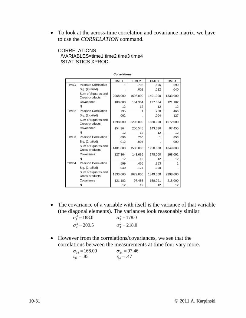
• To look at the across-time correlation and covariance matrix, we haveto use the

CORRELATION command.

CORRELATIONS IABL time1 2 time3 4 TIST XPRO

/VAR /STA

ES= timeD

timeICS .

Correlations

1 .795 .696 .599. .002 .012 .040

2068.000 1698.000 1401.000 1333.000

188.000 154.364 127.364 121.18212 12 12 12

.795 1 .760 .466

.002 . .004 .127

1698.000 2206.000 1580.000 1072.000

154.364 200.545 143.636 97.45512 12 12 12

.696 .760 1 .853

.012 .004 . .000

1401.000 1580.000 1958.000 1849.000

127.364 143.636 178.000 168.09112 12 12 12

.599 .466 .853 1

.040 .127 .000 .

1333.000 1072.000 1849.000 2398.000

121.182 97.455 168.091 218.00012 12 12 12

P n Correlatioearso nSig. (2-tailed)Sum of Cross-products

Squares and

CovarianceN

TIME1 TIME2 TIME3 TIME4TIME1

P n Correlatioearso nSig. (2-tailed)S Squares aCross-products

um of nd

CovarianceNPearson CorrelationSig. (2-tailed)

TIME2

Sum of Squares andCross-productsCovarianceNPearson CorrelationSig. (2-tailed)Sum of Squares and

TIME3

Cross-productsCovariance

TIME4

N

• The covariance of a variable with itself is the variance of that variable (the diagonal elements). The variances look reasonably similar

σ12 =188.0

σ22 = 200.5

σ3

2 =178.0σ4

2 = 218.0

• However from the correlations/covariances, we see that the

correlations between the measurements at time four vary more. σ34 =168.09 σ24 = 97.46 r34 = .85 r24 = .47


o In 1970, several researchers discovered that compound symmetry is

actually an overly restrictive assumption.

• e no assumption about the ariances. In fact, we did not use the

variances of the time 1 and time 2 data. However, we did compute a

Recall that for the paired t-test, we madhomogeneity of the two v

variance of the difference of the paired data.

• The same logic applies to a more general repeated measures design. We are actually concerned about the variance of the difference of observations across the time periods.

• Earlier, we used the following formula for the variance of the

difference of two variables: σX1− X2

2 = σX1

2 + σX 2

2 − 2ρ12σ X1σX 2

• If we have compound symmetry, then and ρij = ρσX i

2 =σ X j

2 =σ 2 so that we can write:

σXi − X j

2 =σ 2 +σ 2 −2ρ σ σ

There are no subscripts on the right side of the equation. In other words, under compound symmetry the variance of the difference of any two variables is the same for all variables.

• The assumption that the variance of the difference of all variables is a

constant is known as sphericity. Technically, it is the assumption of sphericity that we need to satisfy for repeated measures ANOVA.

• If you satisfy the assumptions of compound symmetry, then you

automatically satisfy the sphericity assumption. However it is possible (but rather rare) to satisfy sphericity but not the compound

(For you math-heads, compoundcondition, but not a necessary condition)

symmetry assumption.

symmetry is a sufficient


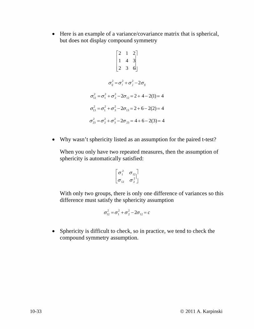
• Here is an example of a variance/covariance matrix that is spherical,

but does not display compound symmetry

⎥⎥⎥

⎦⎢⎢⎢

⎣ 632341

⎤⎡ 212

σ ij2 =σ i

2 +σ j2 −2σ ij

σ12

2 =σ12 +σ 2

2 −2σ12 = 2 + 4 − 2(1) = 4

σ132 =σ1

2 +σ 32 −2σ13 = 2 + 6 − 2(2) = 4

σ23

2 =σ 22 +σ 3

2 −2σ 23 = 4 + 6 − 2(3) = 4

• Why wasn’t sphericity listed as an assumption for the paired t-test?

have two repeated measures, then the assumption of

When you onlysphericity is automatically satisfied:

⎥⎦

⎤⎢⎣

⎡22

With only two groups, there is only one difference of variances so this

12

1221

σσσσ

difference must satisfy the sphericity assumption

σ122 =σ1

2 +σ 22 −2σ12 = c

e • Sphericity is difficult to check, so in practice, we tend to check th

compound symmetry assumption.


• To recap, the assumptions we have to check for a repeated measures design are: o Participants are independent and randomly selected from the population o Normality (actually symmetry) o Sphericity (In practice, compound symmetry)

• SPSS prints a few tests of sphericity, but due to the assumptions required of these tests, they are essentially worthless and you should not rely upon them at all.

• What can I do when the assumptions are violated? o Transformations are of little use due to the complicated nature of the

variance/covariance matrix

o One possibility is the non-parametric, rank-based Friedman test. The Friedman test is appropriate for one-factor within-subjects design. (However, non-parametric alternatives are not available for multi-factor

factors) •

• onsider n participants measured at a different times. • For each subject, replace the observation by the rank of the

observation

Ori

a

within-subjects designs or for designs with both within and between

Does not require normality or any assumption of variances

C

ginal Data

Age (Months) Subject 30 36 42 48 1 108 96 110 122 2 103 117 127 133

Ranked Data

Age (Months) Subject 30 36 42 48 1 2 1 3 4 2 1 2 3 4

• Conceptually, you then perform a repeated-measures ANOVA on the

ranked data • SPSS performs this test and gives a chi-square statistic and p-value


o In multi-factor designs, the rank-based test less useful. Thus, in many

ariance assumption. Many ption

n the variances across groups in a oneway

sythe correction for

situations you are left with three options:

• Play dumb and ignore the violation of the vpeople use this option. Unfortunately, when the sphericity assumis violated, the actual Type I error rate will be inflated

• Use an adjusted test. Whedesign were not equal, we used a Brown-Forunequal variances. The BF adjustment corrected the degrees of freedom to correct for the unequal variances. Two such adjustments exist for the repeated measures case: ˜ ε and ˆ ε .

• Reject the ANOVA approach to repeated measures altogether and

for a MANOVA approach. This approach makes no assumptions on the variance/covariance matrix and is favored by many statisticians. Unfortunately, the MANOVA approach is beyond the scope of this

go

far a variance/covariance matrix

hericity,

class.

• Corrected repeated measures ANOVA and when to use them:

o In 1954 Box derived a measure of howdeparts from sp ε.

xactly satisfy the sphericity assumption, If the data e ε = 1 If are no pherica the data t s l, then ε < 1.

The greater ε departs from 1, the greater the departure from sphericit

adjust a standard F-test to correct

hericity.

y

Box also showed that it was possible tofor the non-sp

df =NUM ε(a −1)df 1)

a = Levels of the repeated measure variablen umber o ticipant

DEN =ε(a −1)(n − = n f par s

At the time, Box did not know how to estimate ε. Since that time, three estimates have been proposed.

nhouse’s (1959)• The Lower-Bound Adjustment • Geisser-Gree ˆ ε • Huynh-Feldt’s (1976) ˜ ε


o In 1958 Geisser-Greenhouse showed that if the repeated-measure

variable had a levels, then ε could be no lower than 1(a −1)

. This is the

lower bound estimate of ε. SPSS prints the lower-bound estimate, but more recently, it has become possible to estimate ε. Thus, the lower-bound estimate is out-of-date and should never be used.

o Geisser-Greenhouse (1959) developed a refinement of Box’s estimate of

ε, called ˆ ε . ˆ ε controls the Type I error rate, but tends to be overly conservative by underestimating ε.

o Huynh-Feldt’s (1976) ˜

ε slightly overestimates ε, and in some cases can lead to a slightly inflated Type I error rate, but this overestimate is very

small.

o In most cases, ˆ ε and ˜ ε give very similar results, but when they differ most statisticians (except Huynh & Feldt) prefer to use ˆ ε

• Of the three options available in SPSS, the Geisser-Greenhouse ε̂ is the best bet. Remember that ε̂ is an adjustment when sphericity is not a valid

the F-test. Here is a general rule of thumb:

assumption in the data. If the data deviate greatly from being spherical, thenit may not be possible to correct

ε̂ > .9 The sphericity assumption is satisfied, no correction necessary

.9 > ε̂ > .7 The sphericity assumption is not satisfied, use the GG ε̂ correction

)1)(1(ˆ)1(ˆ

−−=−=

nadfadf NUM

εε

DEN

.7 > ε̂ The sphericity assumption is not satisfied, and it is violated so

severely that correction is not possible. You should switch to

ations of sphericity, but they still tion.

the MANOVA approach to repeated measures or avoid omnibus tests

o These tests can adjust for minor violrequire the normality assump


• Let’s look at our age example. By visually examining the

variance/covariance matrix, we noticed that the data did not exhibit compound symmetry. Let’s see if looking at the estimates of ε confirm our suspicions.

Mauchly's Test of Sphericity

Measure: MEASURE_1

.243 13.768 5Within Subjects EffectTIME

Mauchly's WApprox.

Chi-Square df.018 .610 .725 .333

Sig.Greenhouse-Geisser Huynh-Feldt

Epsilona

Lower-bound

Tests the null hypothesis that the error covariance matrix of the orthonormalized transformed dependent variables isproportional to an identity matrix.

May be used to adjust the degrees of freedom for the averaged tests of significance. Corrected tests are displayed in theTests of Within-Subjects Effects table.

a.

In this case both

DO NOT use Mauchly’s test of Sphericity. It is not a reliable test.

ˆ ε and ˜ ε converge to the same conclusion. We do not have sphericity in this data. We can now use ˆ ε to construct an adjusted F-test.

• To apply the ε̂ correction, we use the unadjusted F-value, however, we correct the numerator and denominator degrees of freedom

)1(ˆ −= adf NUM

)1)(1(ˆ −−= nadf εε

DEN

For the age d ives us the following analyses:

ata, SPSS g


Measure: MEASURE_1

552.000 3 184.000 3.027 .043552.000 1.829 301.865 3.027 .075552.000 2.175 253.846 3.027 .064552.000 1.000 552.000 3.027 .110

2006.000 33 60.7882006.000 20.115 99.7272006.000 23.920 83.8632006.000 11.000 182.364

Type III Sumof Squares df Mean Square F Sig.Source

Sphericity AssumedGreenhouse-GeisserHuynh-FeldtLower-bound

TIME


Error(TIME)


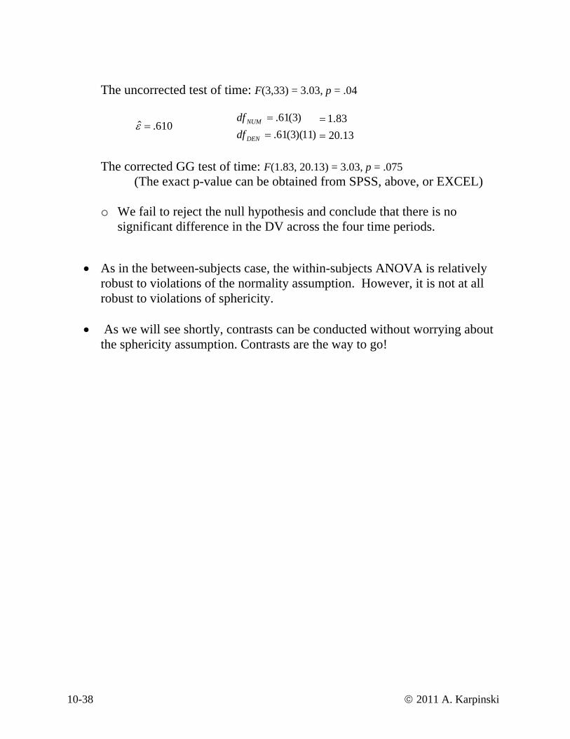
The uncorrected test of time: F(3,33) = 3.03, p = .04

610.ˆ =ε )3(61.=NUMdf 83.1

)11)(3(61.=DENdf 13.20==

The corrected GG test of time: F(1.83, 20.13) = 3.03, p = .075

(The exact p-value can be obtained from SPSS, above, or EXCEL)

o We fail to reject the null hypothesis and conclude that there is no significant difference in the DV across the four time periods.

• As in the between-subjects case, the within-subjects ANOVA is relatively robust to violations of the normality assumption. However, it is not at all rob

• As l t

the

ust to violations of sphericity.

we will see short y, contrasts can be conducted without worrying abou sphericity assumption. Contrasts are the way to go!


9. Co

• In a repeated measures design, MSE is an omnibus error term, computed across all the repeated-measures. If there are a repeated-measures, then the

SE is an average of (a-1) error terms! contrasts run on

thecomputed.

peated-

o Let’s look at an example with our age data. Here is the within-subject contrast table printed by default in SPSS

ntrasts

Mo The (a-1) error terms are determined by (a-1) orthogonal

a repeated-measures. An error term specific to each contrast is

o The default in SPSS is to conduct polynomial contrasts on the a remeasures.

GLM time1 time2 time3 time4 /WSFACTOR = time 4 Polynomial


Measure: MEASURE_1

540.000 1 540.000 5.024 .04712.000 1 12.000 .219 .649

.000 1 .000 .000 1.0001182.400 11 107.491

604.000 11 54.909219.600 11 19.964

TIMEType III Sum

Source df Mean Square F Sig.of SquaresLinearQuadraticCubic

TIME

LinearQuadratic

Error(TIME)

Cubic

• Note that there are three separate error terms, each with 11 df

Error (Linear) 107.491 Error (Quad) 54.909 Error (Cubic) 19.964

• If we take the average of these three terms, we obtain the MSE with

33 df: 788.60

3964.19909.54491.107

=++


Measure: MEASURE_1

552.000 3 184.000 3.027 .0432006.000 33 60.788

Sphericity AssumedSphericity Assumed

SourceTIMEError(TIME)



formulae for contrasts are the same as for a one-way ANOVA: o The

=observedt ∑

∑′ nEMS j

=′

Xc jj .)ˆ(rerro standard

ˆψ

ψ c 2

SS ˆ ψ =

∑ njc 2

2 ψ̂ EMS

SSfdF =′′

ψ̂),1(

•

• We have two choices for

The only difference is that MSE has been replaced by EMS ′

EMS ′

o Use the omnibus with df = (a-1)(n-1)

When the sphericity assumption is satisfied, each of the separate

error terms should be identical. They all estimate the true error variance

In this case, using the omnibus MSE results in greater power due to the increased denominator degrees of freedom

In practice, the loss of power due to a decrease in the degrees of

freedom is offset by having a more accurate error term

ption, most statisticians recommend you always use the contrast-specific error term

• Unfortunately, calculating the contrast-specific error term is tedious. I will provide a few different methods to avoid any hand-calculations.

MSE

o Use the contrast-specific error term with df = (n-1)

Due to the problems of the sphericity assumption and the difficulties in checking this assum


• nderstanding repeated-measures contrasts

o These repeated-measures contrasts operate on the marginal repeated-factor means, collapsing across the participants

U

o In our infant growth example, we have four repeated measures. With four observations, we can conduct 3 single-df tests. Let’s examine the polynomial trends:

ths)

Age (Mon 30 36 42 48 Average 103 107 110 112 Linear -3 -1 1 3 Quad 1 -1 -1 1 Cubic -1 3 -3 1

30)112)(3()110)(1()107)(1()103(3ˆ +−+−=linψ =+

54020

900 30)ˆ( 2222

2

==−−linSS ψ

1212121212 ⎠⎝

2)112)(1()110)(1()107)(1()103(1

)3()1()1()3(⎟⎞

⎜⎛+++

ˆ −=+−+−+=quadψ

ˆ 0)112)(1()110)(3()107)(3()103(1 =+−++−=cubψ

• : Method 1Computing the error term Using SPSS’s built-in, brand-name contrasts o Reme is one of

those con

• ifference

mber SPSS’s built-in contrasts? If your contrast of interest trasts, you can ask SPSS to print the test of the contrast

D : Each level of a factor is compared to the mean of the previous levels

• Helmert: Each level of a factor is compared to the mean of subsequent levels

• Polynomial: Uses the orthogonal polynomial contrasts • Repeated: Each level of a factor is compared to the previous level • Simple: Each level of a factor is compared to the last level


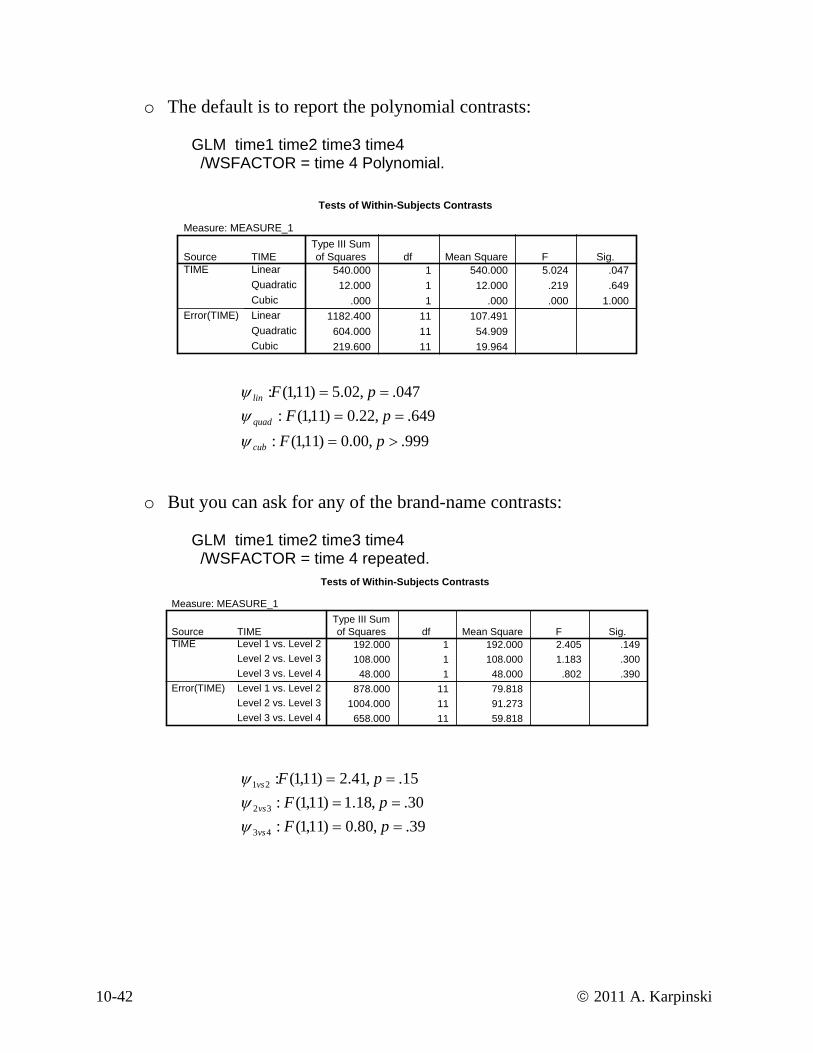
o The default is to report the polynomial contrasts: GLM time1 time2 time3 time4 /WSFACTOR = time 4 Polynomial.


Measure: MEASURE_1

540.000 1 540.000 5.024 .04712.000 1 12.000 .219 .649

.000 1 .000 .000 1.0001182.400 11 107.491

604.000 11 54.909219.600 11 19.964

TIMELinear

Type III Sum

QuadraticCubic

SourceTIME

df Mean Square F Sig.of Squares

LinearQuadraticCub

Error(TIME)

ic

047.,02.5)11,1(: == pFlin ψ

649.,22.0)11,1(: == pFquadψ 999.,00.0)11,1(: >= pFcubψ

o But you can ask for any of the brand-name contrasts:

LM time1 time2 time3 time4 OR = time 4 repeated.

G /WSFACT


Measure: MEASURE_1

192.000 1 192.000 2.405 .149108.000 1 108.000 1.183 .300

48.000 1 48.000 .802 .390878.000 11 79.818

1004.000 11 91.273658.000 11 59.818

TIMEType III Sumof SquaresSource df Mean Square F Sig.

Level 1 vs. Level 2Level 2 vs. Level 3Level 3 vs. Level 4

TIME

Level 1 vs. Level 2Level 2 vs. Level 3

Error(TIME)

Level 3 vs. Level 4

15.,41.2)11,1(:21 == pFvsψ 30.,18.1)11,1(:32 == pFvsψ

1,1(: F 39.,80.0)1 == p 43ψ vs


• Computing the error term: Method 2 Using SPSS’s “special” contrast

comm

o Instead of specifying a set of brand-name contrasts, you can enter a set of contrasts.

o You must

and

first enter a contrast of all 1’s o You then must enter (a-1) contrasts

o For example, let’s ask for the polynomial contrasts using the “special”

command: GLM time1 time2 time3 time4 /WSFACTOR = time 4 special ( 1 1 1 1 -3 -1 1 3 1 -1 -1 1 -1 -3 1).

3


Measure: MEASURE_1

10800.000 1 10800.000 5.024 .04748.000 1 48.000 .219 .649

.000 1 .000 .000 1.00023648.000 11 2149.8182416.000 11 219.6364392.000 11 399.273

TIMEL1

Type III Sumof Squares df Mean Square F

L2L3

SourceTIME

Sig.

L1L2

Error(TIME)

L3

L1 is the linear trend: 047.,02.5)11,1(: == pFlinψ L2 is the quadratic trend: 649.,22.0)11,1(: == pFquadψ

99.,00.0)11,1(: >= pFcubψ L3 is the cubic trend:

o If all of your contrasts are not ortho-normalized (the set of contrasts is orthogonal, and the sum of the squared contrast coefficients equal 1), then the calculation of the SS will be disturbed, but the F-value and the significance test will be ok.


o Now, let’s consider a more complicated set of contrasts

FACTOR = time 4 special (1 1 1 1 -1 -1 2 0

GLM time1 time2 time3 time4 /WS -1 0 2 -1 0 -1 2 -1)


Measure: MEASURE_1

1200.000 1 1200.000 3.689 .081300.000 1 300.000 1.680 .221

12.000 1 12.000 .153 .7033578.000 11 325.2731964.000 11 178.545

864.000 11 78.545

TIMEL1L2L3L1L2L3

SourceTIME

Error(TIME)


1 is (time 1 and time 2) vs. time 3, 08.,69.3)11,1( == pF LL2 is (time 1 and time 4) vs. time 3, 22.,68.1)11,1( == pF L3 is (time 2 and time 4) vs. time 3, 70.,15.0)11,1( == pF

o To use the special command, you need to remember to enter the contrast

of all 1’s and a set of (a-1) contrasts.

• Computing the error term: Method 3 Compute the value of the contrast as a

new v am le t-test on that variable to tes for a differe

o Again, let’s start by replicating the polynomial contrasts using this

method:

ariable, and run a one-s p t nce from zero

compute lin = -3*time1 - time2 + time3 + 3*time4. compute quad = time1 - time2 - time3 + time4. compute cubic = -time1 +3* time2 -3*time3 + time4.


T-TEST /TESTVAL=0 /VARIABLES=lin.

One-Sample Test

2.241 11 .047 30.0000 .5404 59.4596LINt df Sig. (2-tailed)

MeanDifference Lower Upper

Test Value = 095% Confidence

Interval of theDifference

047.,02.5)11,1(: == pFlinψ 047.,24.2)11(: == ptlinψ

o The advantage of this procedure is that you can test any contrast one-at-a-time

o Th . When we run a c ntrast, we

col ethod, we create a new variable ref ch participant. We en collapse across participants, average all contrast values, and test to see if this

at are easily interpretable

u can rasts before looking at the data.

is method should make intuitive sense olapse across participants. With this mlecting the value of the contrast for ea th

average contrast differs from zero!

• So for repeated-measures designs, if we only run contrasts: o We can discard the sphericity assumption o We can run tests th

o The catch is that you need to have strong enough predictions that yo

plan cont


Planned a• Remember that with all the controversy surrounding the assumptions for a

repeated-measures design, you should try very hard to avoid omnibus tests and conduct all your analyses using single-df tests.

• The logic for planned and post-hoc tests for a one-factor within-subjects

design parallels the logic for a one-factor between-subjects design

o When there are a repeated-measures, the unadjusted omnibus test has (a-1) dfs

If you decide to forgo the omnibus test, then you can use those (a-1) dfs to

I believe that in the presence of a strong theory, you may conduct (a-1)

ou roni or Dunn-Sidák correction:

Dunn/Sidák Bonferroni

10. nd post-hoc tests

o

conduct (a-1) orthogonal, planned contrasts.

planned contrasts, even if they are not orthogonal.

• If you first conduct the omnibus test, or if you plan more than (a-1) contrasts, then you need to adjust your p-values to correct for the number of tests yare conducting, using either the Bonfer

ccritp

1

)1(1 α−−= c

pcritα

=

• Unfortunately, using contrast-specific error terms make controlling the type-

dák as a post-hoc procedure

• For pairwise comparisons, you must let C = the total number of possible pairwise comparisons

• If you have a groups, then

1 error for post-hoc tests very difficult. If each contrast has a different error term, then the logic of the Tukey and Scheffé procedures breaks down. The only good option is this case is to use Bonferroni/Dunn-Si

C =a(a −1)

2

• For pairwise and complex comparisons, you must let C = the total number of possible pairwise comparisons + the number of complex comparisons conducted.


• As an example, let’s conduct all pairwise comparisons in the age data. In SPSS, you can ask for Bonferroni comparisons on the marginal within-subjects means.

GLM time1 time2 time3 time4 /WSFACTOR=time 4 Polynomial /EMMEANS=TABLES(time) COMPARE ADJ(BONFERRONI) /PRINT=DESCRIPTIVE.


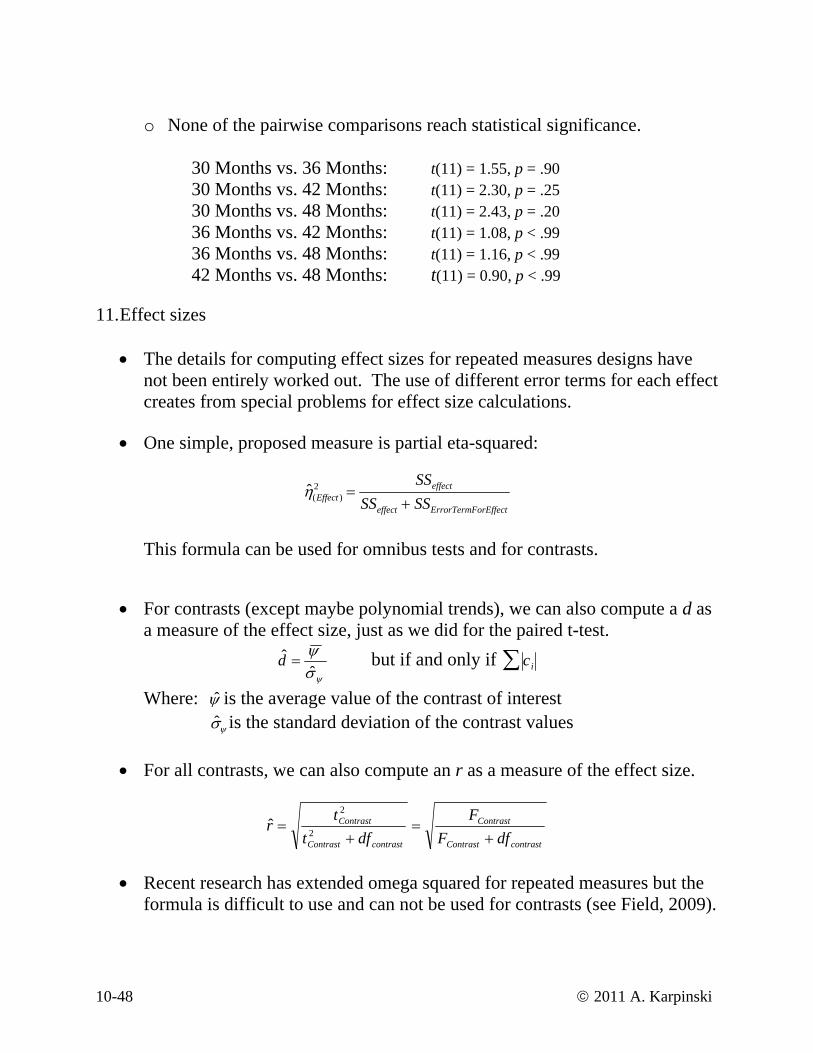
o None of the pairwise comparisons reach statistical significance.

vs. 42 Months: t(11) = 2.30, p = .25 30 Months vs. 48 Months: t(11) = 2.43, p = .20

t p < .99

Effect sizes

• The details for computing effect sizes for repeated measures designs have not been entirely worked out. The use of different error terms for each effect creates from special problems for effect size calculations.

• One simple, proposed measure is partial eta-squared:

30 Months vs. 36 Months: t(11) = 1.55, p = .90 30 Months

36 Months vs. 42 Months: (11) = 1.08, 36 Months vs. 48 Months: t(11) = 1.16, p < .99

: t(11) = 0.90, p < .99 42 Months vs. 48 Months 11.

ˆ η (Effect )2 =

SSeffect

SSeffect + SSErrorTermForEffect

This formula can be used for omnibus tests and for contrasts.

• For contrasts (except maybe polynomial trends), we can also compute a d as a measure of the effect size, just as we did for the paired t-test.

ψσψˆ

ˆ =d but if and only if ci∑

Where: ψ̂ is the average value of the contrast of interest ˆ σ ψ is the standard deviation of the contrast values

• For all contrasts, we can also compute an r as a measure of the effect size.

contrastContrast

Contrast

contrastContrast

Contrast

dfFF

dftt

r+

=+

= 2

2

ˆ

• Recent research has extended omega squared for repeated measures but the

formula is difficult to use and can not be used for contrasts (see Field, 2009).


• Examples of Effect Size Calculations:

o Om

4 nibus test of the within-subject factor: GLM time1 time2 time3 time /WSFACTOR = time 4 Polynomial


Measure: MEASURE_1

552.000 3 184.000 3.027 .043552.000 1.829 301.865 3.027 .075552.000 2.175 253.846 3.027 .064552.000 1.000 552.000 3.027 .110

2006.000 33 60.7882006.000 20.115 99.7272006.000 23.920 83.8632006.000 11.000 182.364

Type III Sumof Squares df Mean Square F


SourceTIME

Sig.


Error(TIME)

22.2006552

ˆ =+

=+

=orTimeErrorTermFTime

Time SSSSη 5522 TimeSS

• Recall that for this example, the sphericity assumption has been

This calculation has been included to show you an example of how to

lation would be unaffected.

22.,04.,03.3)33,3( 2 === ηpF

severely violated. Thus, we should not report this test.

calculate partial eta squared for the omnibus test, but it is not appropriate to report this test.

• If you applied an epsilon adjustment, the effect size calcu


o Polynomial Trends: Partial Eta-Squa

GLM time1 time2 time3 time4 red or r

/WSFACTOR = time 4 Polynomial Tests of Within-Subjects Contrasts

Measure: MEASURE_1

540.000 1 540.000 5.024 .04712.000 1 12.000 .219 .649

.000 1 .000 .000 1.0001182.400 11 107.491

604.000 11 54.909219.600 11 19.964

TIMEType III Sumof SquaresSource df Mean Square F Sig.

LinearQuadraticCubic

TIME

LinearQuadratic

Error(TIME)

Cubic

56.1102.5

02.5=

+=

+=

contrastContrast

ContrastLinear dfF

Fr

14.1122.0

22.0=

+=Quadraticr

31.1182540 ++ orLinearErrorTermFLinear SSSS

542 === LinearLinear

SSη 0

02.60412

122 =+

=+

=corQuadratiErrorTermFQuadratic

QuadraticQuadratic SSSS

SSη

o Pairwise Contrasts: Partial Eta-Squ

ared or d GLM time1 time2 time3 time4 /WSFACTOR = age 4 simple (1).


Measure: MEASURE_1

192.000 1 192.000 2.405 .149588.000 1 588.000 5.284 .042972.000 1 972.000 5.940 .033878.000 11 79.818

1224.000 11 111.2731800.000 11 163.636

ageLevel 2 vs. Level 1Level 3 vs. Level 1Level 4 vs. Level 1Level 2 vs. Level 1Level 3 vs. Level 1Level 4 vs. Level 1

Sourceage

Error(age)


18.878192

192

2121

21221 =

+=

+=

vsorErrorTermFvs

vsvs SSSS

SSη

32.1224588

588231 =

+=vsη 35.

18009729722

41 =+

=vsη


12. A final example

• A rese unt of daylight people are exposed to (She b fects mood). A sample of 110 individuals, all age 60-70, recorded their daily exposure to sunlight over the course of a year. The researcher computed an average daily exposure to sunlight (hours/day) for each of the four seasons, and wanted to test the following hypotheses o Are there any trends in exposure across the seasons? o Is winter the season with the lowest exposure? o Is summer the season with the highest exposure?

• Here is a graph of the data for the first 20 participants

o The overall average exposure is indicated with the dark blue line

archer is interested in the amoelieves that exposure to daylight af

0

2

4

6

8

10

• Each p one factor repeated measures

(within-subjects) design would seem to be appropriate. o Participants are independent and randomly selected from the population o Normality (actually symmetry) o Sphericity

erson is observed each season. A


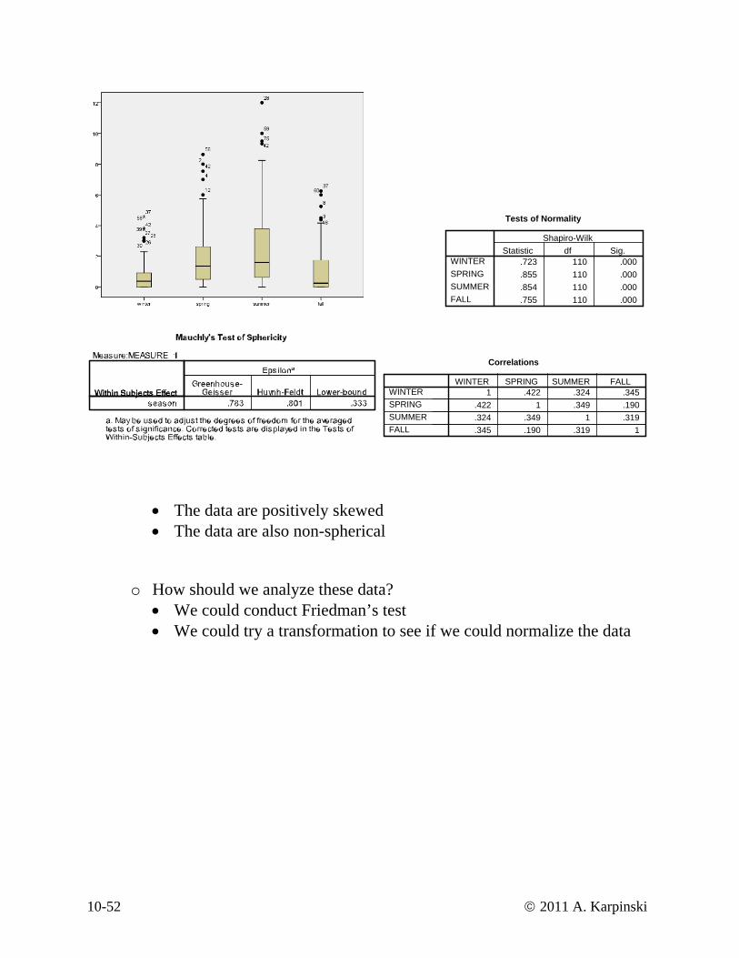
Tests of Normality

.723 110 .000

.855 110 .000

.854 110 .000

.755 110 .000

WINTERSPRINGSUMMERFALL

Statistic dfShapiro-Wilk

Sig.

Correlations

1 .422 .324 .345.422 1 .349 .190.324 .349 1 .319.345 .190 .319 1

WINTERSPRINGSUMMERFALL

WINTER SPRING SUMMER FALL

• The data are positively skewed • The data are also non-spherical

o How should we analyze these data? • We could conduct Friedman’s test • We could try a transformation to see if we could normalize the data


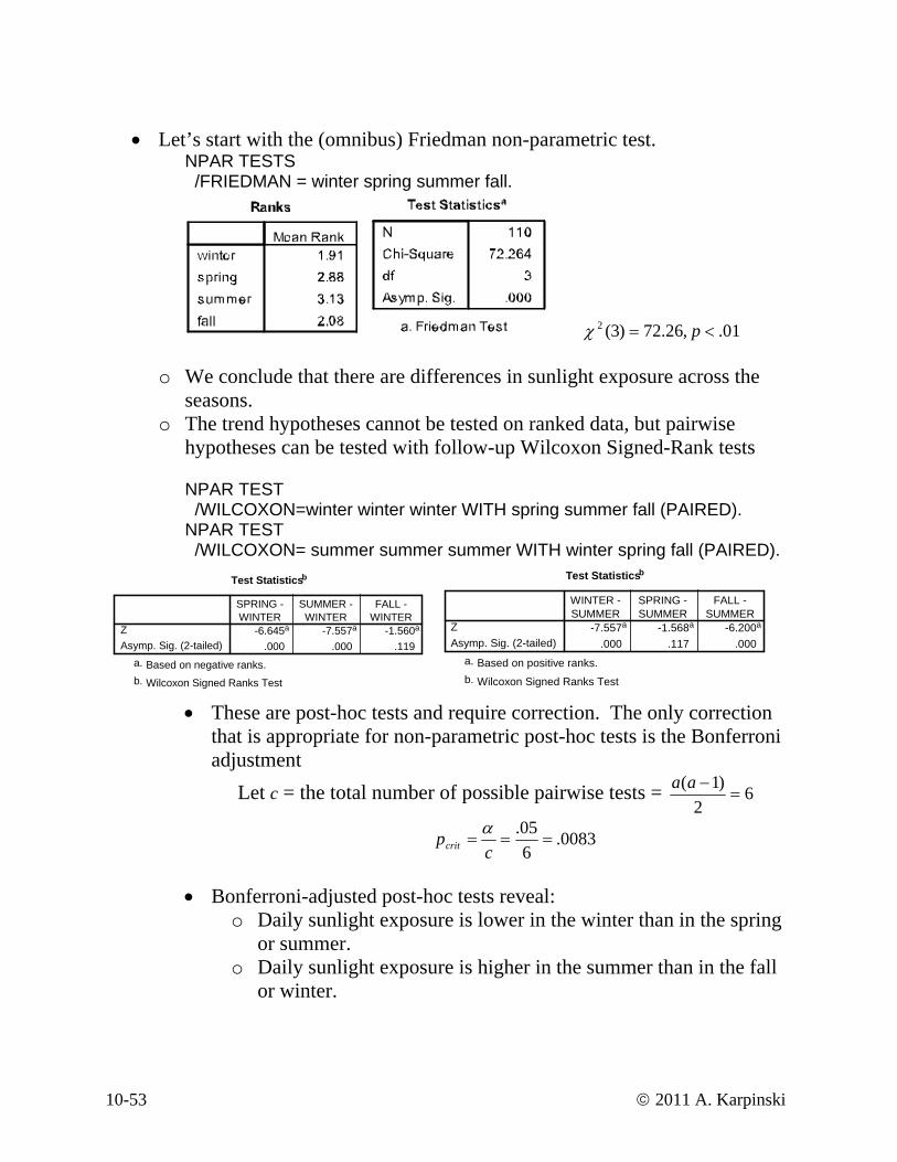
• Let’s start with the (omnibus) Friedman non-parametric test.

NPAR TESTS /FRIEDMAN = winter spring summer fall.

01.,26.72)3(2 <= pχ

o We conclude that there are diffe in ight exposure across the seasons.

o The trend hypotheses cannot be tested on ranked data, but pairwise hypotheses can be tested with follow-up Wilcoxon Signed-Rank tests

NPAR TEST /WILCOXON=winter winter winter WITH spring summer fall (PAIRED). NPAR TEST /WILCOXON= summer summer summer WITH winter spring fall (PAIRED).

rences sunl

Test Statisticsb

-6.645a -7.557a -1.560a

.000 .000 .119ZAsymp. Sig. (2-tailed)

SPRING -WINTER

SUMMER -WINTER

FALL -WINTER

Based on negative ranks.a.


Test Statisticsb

-7.557a -1.568a -6.200a

.000 .117 .000

WINTER -SUMMER

SPRING -SUMMER

FALL -SUMMER

ZAsymp. Sig. (2-tailed)

Based on positive ranks.a.


ire correction. The only correction ic post-hoc tests is the Bonferroni

Let c = the total number of possible pairwise tests =

• These are post-hoc tests and requthat is appropriate for non-parametradjustment

62

)1(=

−aa

0083.605.

===c

pcritα

• Bonferroni-adjusted post-hoc tests reveal:

o Daily sunlight exposure is lower in the winter than in the spring or summer.

o Daily sunlight exposure is higher in the summer than in the fall or winter.


• Alternatively, I could apply a transformation and analyze the transformed start. (Some

participants have scores of zero, tran

Compute srqtwinter = SQRT(winter). Compute srqtspring= SQRT(spring). Compute sqrtsummer = SQRT(summer). Compute sqrtfall = SQRT(fall).

• Let’s check the assumptions on the transforme

data. A square root transformation seems like a good place tomaking it difficult to work with a log

sformation).

d data.

GLM winter spring summer fall /WSFACTOR = season 4 /PRINT = DESC.

o

Normality and sphericity are satisfied.


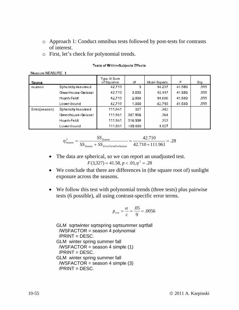
o Approach 1: Conduct omnibus tests followed by post-tests for contrasts of interest.

o First, let’s check for polynomial trends.

28.961.111710.42

710.422 =+

=+

=orSeasonErrorTermFSeason

SeasonSeason SSSS

SSη

• The data are spherical, so we can report an unadjusted test.

• We conclude that there are differences in (the square root of) sunlight exposure across the seasons.

• We follow this test with polynomial trends (three tests) plus pairwise tests (6 possible), all using contrast-specific error terms.

28.,01.,58.41)327,3( 2 =<= ηpF

0056.905.

===c

pcritα

GL er sqrtfall /W omial /P

/PRINT = DESC. GLM winter spring summer fall /WSFACTOR = season 4 simple (3) /PRINT = DESC.

M sqrtwinter sqrtspring sqrtson 4 polyn

ummSFACTOR = seasRINT = DESC.

GLM winter spring summer fall /WSFACTOR = season 4 simple (1)


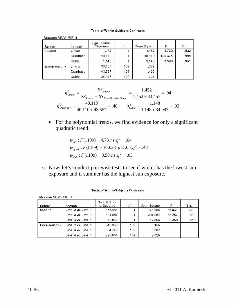
04.457.33452.1

452.12 =+

=+

=orLinearErrorTermFLinear

LinearLinear SSSS

SSη

48.557.43110.40

110.402 =+

=Quadraticη 03.947.34148.1

148.12 =+

=Cubicη

• For the polynomial trends, we find evidence for only a significant

quadratic trend.

04.,,73.4)109,1(: 2 == ηψ nsFlin 48.,05.,38.100)109,1(: 2 =<= ηψ pFquad

03.,,58.3)109,1(: 2 == ηψ nsFcub

ighest sun exposure.

o Now, let’s conduct pair wise tests to see if winter has the lowest sun exposure and if summer has the h


• For pairwise tests, I prefer to report d effect sizes. Information for d effect sizes can be obtained by calculating the contrasts of interest.

COMPUTE WinSpr = sqrtspring- sqrtwinter. COMPUTE WinSum = sqrtsummer- sqrtwinter.

OMPUTE WinFall = sqrtfall- sqrtwinter. E

CD SC VAR = WinSpr WinSum WinFall.


COMPUTE SumWin = sqrtsummer- sqrtwinter. COMPUTE SumSpr = sqrtsummer- sqrtspring. COMPUTE SumFall = sqrtsummer-sqrtfall.

Fall DESC VAR = SumWin SumSpr Sum

77.73561.ˆint ===

ψσ5639.ψ

ervsSpringWd 90.82976.int ==ervsSummerWd 7523. 15.

74285.int ==ervsFallWd 1085.

22.83863.1884.

==ringSummervsSpd 71.89857.6438.

==llSummervsFad 90.82976.7523.

ˆint ===ψσ

ψerSummervsWd

Bonferroni adjusted pairwise tests reveal: o (Log) Daily sunlight exposure is significantly lower in the

winter than in the spring or summer, ds > .77 o Daily sunlight exposure in the fall and winter are not

significantly different, d = .15.

o Daily sunlight exposure is significantly higher in the summer than in the fall or winter, ds > .71

o Daily sunlight exposure in the summer and spring are not significantly different, d = .22.

o Approach 2: Skip the omnibus test. • Conduct uncorrected planned, trend contrasts. • Conduct post-hoc pairwise tests.

• For the polynomial trends, we fiquadratic trend.

nd evidence for only a significant

04.,,73.4)109,1(: 2 == ηψ nsFlin 48.,05.,38.100)109,1(: 2 =<= ηψ pFquad

03.,58.3)109,1(: 2 == η,ψ nsFcub

• Be cautious in interpreting these trends. Seasons are cyclical. If we had started our analyses in the summer, we would obtain different results.


0083.605.

===c

pcritα

Bonferroni adjusted pairwise tests reveal: o (Log) Daily sunlight exposure is significantly lower in the

winter than in the spring or summer, ds > .77 o Daily sunlight exposure in the fall and winter are not

significantly different, d = .15.

o Daily sunlight exposure is significantly higher in the summer than in the fall or winter, ds > .71

o Daily sunlight exposure in the summer and spring are not significantly different, d = .22.

• The two parametric approaches lead to identical conclusions.

• For the polynomial trends, we find evidence for only a significant quadratic trend.


0.00

0.50

1.00

1.50

2.00

2.50

3.00

Winter Spring Summer Fall

Square root of Sun Exposure

Season

Sun Exposure by Season

Error Bars are + 1 StandardError


one-factor repeated measures anova - the home page for astro…andykarp/graduate_statistics... ·...

Documents