CHAPTER

ONE INTRODUCTION

1.1 GENERAL REMARKS The development of the high-speed digital computer during the twentieth century has had a great impact on the way principles from the sciences of fluid mechanics and heat transfer are applied to problems of design in modern engineering practice. Problems that would have taken years to work out with the computational methods and computers available 30 years ago can now be solved at very little cost in a few seconds of computer time. The ready availability of previously unimaginable computing power has stimulated many changes. These were first noticeable in industry and research laboratories, where the need to solve complex problems was the most urgent. More recently, changes brought about by the computer have become evident in nearly every facet of our daily lives. In particular, we find that computers are widely used in the educational process at all levels. Many a child has learned to recognize shapes and colors from mom and dad’s computer screen before they could walk. To take advantage of the power of the computer, students must master certain fundamentals in each discipline that are unique to the simulation process. It is hoped that the present textbook will contribute to the organization and dissemination of some of this information in the fields of fluid mechanics and heat transfer.

Over the past half century, we have witnessed the rise to importance of a new methodology for attacking the complex problems in fluid mechanics and heat transfer. This new methodology has become known as computational fluid dynamics (CFD). In this computational (or numerical) approach, the equations (usually in partial differential form) that govern a process of interest are solved

3

4 FUNDAMENTALS

numerically. Some of the ideas are very old. The evolution of numerical methods, especially finite-difference methods for solving ordinary and partial differential equations, started approximately with the beginning of the twentieth century. The automatic digital computer was invented by Atanasoff in the late 1930s (see Gardner, 1982; Mollenhoff, 1988) and was used from nearly the beginning to solve problems in fluid dynamics. Still, these events alone did not revolutionize engineering practice. The explosion in computational activity did not begin until a third ingredient, general availability of high-speed digital computers, occurred in the 1960s.

Traditionally, both experimental and theoretical methods have been used to develop designs for equipment and vehicles involving fluid flow and heat transfer. With the advent of the digital computer, a third method, the numerical approach, has become available. Although experimentation continues to be important, especially when the flows involved are very complex, the trend is clearly toward greater reliance on computer-based predictions in design.

This trend can be largely explained by economics (Chapman, 1979). Over the years, computer speed has increased much more rapidly than computer costs. The net effect has been a phenomenal decrease in the cost of performing a given calculation. This is illustrated in Figure 1.1, where it is seen that the cost of performing a given calculation has been reduced by approximately a factor of 10 every 8 years. (Compare this with the trend in the cost of peanut butter in the past 8 years.) This trend in the cost of computations is based on the use of the best serial or vector computers available. It is true not every user will have easy access to the most recent computers, but increased access to very capable computers is another trend that started with the introduction of personal computers and workstations in the 1980s. The cost of performing a calculation on a desktop machine has probably dropped even more than a factor of 10 in an 8-year period, and the best of these “personal” machines are more capable than the best “mainframe” machines of a decade ago, achieving double-digit megaflops (millions of floating point operations per second). There seems to be

1 650 7094 ’-- I I B M 360-50

O O l t -4‘‘ LKHY YHP

--0 1/10 EACH 8 YRS -.%RAY c90

I 1 I I I I I I , --\-

1955 1960 1965 1970 1975 1980 1985 1990 1 35 YEAR NEW COMPUTER AVAILABLE -

Figure 1.1 Trend of relative computation cost for a given flow and algorithm (based on Chapman, 1979; Kutler et al., 1987; Holst et al., 1992; Simon, 1995).

INTRODUCTION 5

no real limit in sight to the computation speed that can be achieved when massively parallel computers are considered. Work is in progress toward achieving the goal of performance at the level of teraflops (10” floating point operations per second) by the twenty-first century. This represents a 1000-fold increase in the computing speed that was achievable at the start of the 1990s. The increase in computing power per unit cost since the 1950s is almost incomprehensible. It is now possible to assign a homework problem in CFD, the solution of which would have represented a major breakthrough or could have formed the basis of a Ph.D. dissertation in the 1950s or 1960s. On the other hand, the costs of performing experiments have been steadily increasing over the same period of time.

The suggestion here is not that computational methods will soon completely replace experimental testing as a means to gather information for design purposes. Rather, it is believed that computer methods will be used even more extensively in the future. In most fluid flow and heat transfer design situations it will still be necessary to employ some experimental testing. However, computer studies can be used to reduce the range of conditions over which testing is required.

The need for experiments will probably remain for quite some time in applications involving turbulent flow, where it is presently not economically feasible to utilize computational models that are free of empiricism for most practical configurations. This situation is destined to change eventually, since it has become clear that the time-dependent Navier-Stokes equations can be solved numerically to provide accurate details of turbulent flow. Thus, as computer hardware and algorithms improve, the frontier will be pushed back continuously allowing flows of increasing practical interest to be computed by direct numerical simulation. The prospects are also bright for the increased use of large-eddy simulations, where modeling is required for only the smallest scales.

In applications involving multiphase flows, boiling, or condensation, es- pecially in complex geometries, the experimental method remains the primary source of design information. Progress is being made in computational models for these flows, but the work remains in a relatively primitive state compared to the status of predictive methods for laminar single-phase flows over aerodynamic bodies.

1.2 COMPARISON OF EXPERIMENTAL, THEORETICAL, AND COMPUTATIONAL APPROACHES As mentioned in the previous section, there are basically three approaches or methods that can be used to solve a problem in fluid mechanics and heat transfer. These methods are

1. Experimental 2. Theoretical

6 FUNDAMENTALS

3. Computational (CFD)

The theoretical method is often referred to as an analytical approach, while the terms computational and numerical are used interchangeably. In order to illustrate how these three methods would be used to solve a fluid flow problem, let us consider the classical problem of determining the pressure on the front surface of a circular cylinder in a uniform flow of air at a Mach number (M,) of 4 and a Reynolds number (based on the diameter of the cylinder) of 5 X lo6.

In the experimental approach, a circular cylinder model would first need to be designed and constructed. This model must have provisions for measuring the wall pressures, and it should be compatible with an existing wind tunnel facility. The wind tunnel facility must be capable of producing the required free stream conditions in the test section. The problem of matching flow conditions in a wind tunnel can often prove to be quite troublesome, particularly for tests involving scale models of large aircraft and space vehicles. Once the model has been completed and a wind tunnel selected, the actual testing can proceed. Since high-speed wind tunnels require large amounts of energy for their operation, the wind tunnel test time must be kept to a minimum. The efficient use of wind tunnel time has become increasingly important in recent years with the escalation of energy costs. After the measurements have been completed, wind tunnel correction factors can be applied to the raw data to produce the final wall pressure results. The experimental approach has the capability of producing the most realistic answers for many flow problems; however, the costs are becoming greater every day.

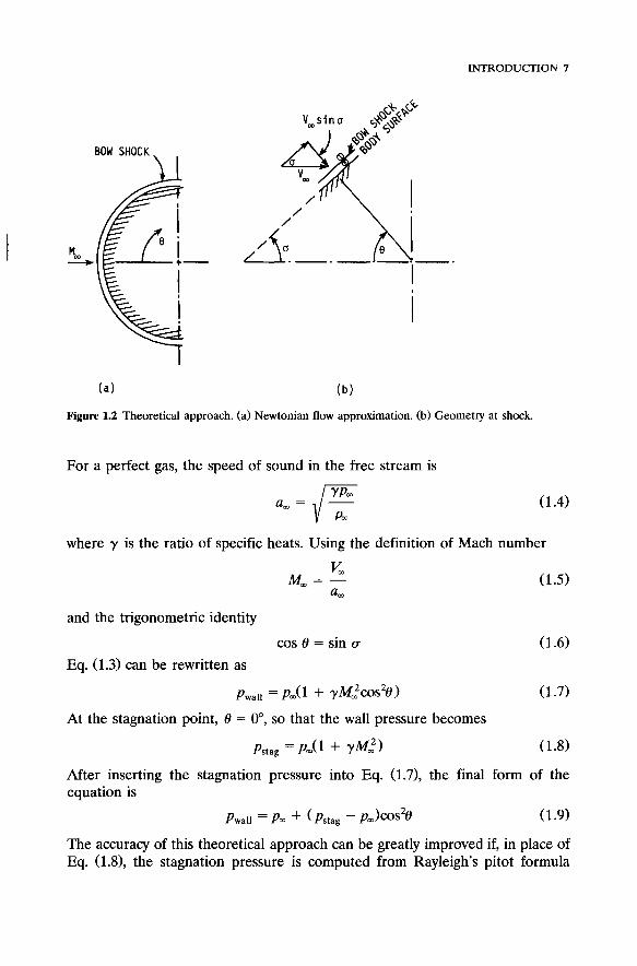
In the theoretical approach, simplifying assumptions are used in order to make the problem tractable. If possible, a closed-form solution is sought. For the present problem, a useful approximation is to assume a Newtonian flow (see Hayes and Probstein, 1966) of a perfect gas. With the Newtonian flow assumption, the shock layer (region between body and shock) is infinitesimally thin, and the bow shock lies adjacent to the surface of the body, as seen in Fig. 1.2(a). Thus the normal component of the velocity vector becomes zero after passing through the shock wave, since it immediately impinges on the body surface. The normal momentum equation across a shock wave (see Chapter 5 ) can be written as

(1.1) where p is the pressure, p is the density, u is the normal component of velocity, and the subscripts 1 and 2 refer to the conditions immediately upstream and downstream of the shock wave, respectively. For the present problem [see Fig. 1.2(b)], Eq. (1.1) becomes

P1 + P I 4 =P2 + P 2 4

0

P m + W~2sin2a = P w a l l + Pwa11+11 (1.2)

or

1 Pa pwall = p , 1 + --I/,'sin2a i P m

INTRODUCTION 7

( a ) ( b )

Figure 1.2 Theoretical approach. (a) Newtonian flow approximation. (b) Geometry at shock.

For a perfect gas, the speed of sound in the free stream is

a, = (1.4)

where y is the ratio of specific heats. Using the definition of Mach number

v, M, = -

am

and the trigonometric identity

cos 9 = sin u Eq. (1.3) can be rewritten as

Pwall =pm(l + yM,2cos29)

(1.5)

(1.6)

(1.7)

At the stagnation point, 9 = O", so that the wall pressure becomes

Pstag = Pm(1 + YM?) (1.8)

After inserting the stagnation pressure into Eq. (1.7), the final form of the equation is

Pwall = P m + (Pstag - P,)COS*~ (1.9)

The accuracy of this theoretical approach can be greatly improved if, in place of Eq. ( 1 8 , the stagnation pressure is computed from Rayleigh's pitot formula

8 FUNDAMENTALS

(Shapiro, 1953):

which assumes an isentropic compression between the shock and body along the stagnation streamline. The use of Eq. (1.9) in conjunction with Eq. (1.10) is referred to as the modified Newtonian theory. The wall pressures predicted by this theory are compared in Fig. 1.3 to the results obtained using the experimental approach (Beckwith and Gallagher, 1961). Note that the agreement with the experimental results is quite good up to about f35”. The big advantage of the theoretical approach is that “clean,” general information can be obtained, in many cases, from a simple formula, as in the present example. This approach is quite useful in preliminary design work, since reasonable answers can be obtained in a minimum amount of time.

In the computational approach, a limited number of ‘assumptions are made and a high-speed digital computer is used to solve the resulting governing fluid dynamic equations. For the present high Reynolds number problem, inviscid flow can be assumed, since we are only interested in determining wall pressures on the forward portion of the cylinder. Hence the Euler equations are the appropriate governing fluid dynamic equations. In order to solve these equations, the region between the bow shock and body must first be subdivided into a computational grid, as seen in Fig. 1.4. The partial derivatives appearing in the

0 EXPERIMENTAL THEORETICAL NUMERICAL ---

ANGLE, e

Figure 13 Surface pressure on circular cylinder.

INTRODUCTION 9

Figure 1.4 Computational grid.

unsteady Euler equations can be replaced by appropriate finite differences at each grid point. The resulting equations are then integrated forward in time until a steady-state solution is obtained asymptotically after a sufficient number of time steps. The details of this approach will be discussed in forthcoming chapters. The results of this technique (Daywitt and Anderson, 1974) are shown in Fig. 1.3. Note the excellent agreement with experiment.

In comparing the methods, we note that a computer simulation is free of some of the constraints imposed on the experimental method for obtaining information upon which to base a design. This represents a major advantage of the computational method, which should be increasingly important in the future. The idea of experimental testing is to evaluate the performance of a relatively inexpensive small-scale version of the prototype device. In performing such tests, it is not always possible to simulate the true operating conditions of the prototype. For example, it is very difficult to simulate the large Reynolds numbers of aircraft in flight, atmospheric reentry conditions, or the severe operating conditions of some turbomachines in existing test facilities. This suggests that the computational method, which has no such restrictions, has the potential of providing information not available by other means. On the other hand, computational methods also have limitations; among these are computer storage and speed. Other limitations arise owing to our inability to understand and mathematically model certain complex phenomena. None of these limitations of the computational method are insurmountable in principle, and current trends show reason for optimism about the role of the computational

10 FUNDAMENTALS

Table 1.1 Comparison of approaches

Approach Advantages Disadvantages

Experimental 1. Capable of being most realistic 1. Equipment required 2. Scaling problems 3. Tunnel corrections 4. Measurement difficulties 5. Operating costs

1. Restricted to simple geometry and physics

2. Usually restricted to linear problems

Theoretical 1. Clean, general information, which is usually in formula form

Computational 1. No restriction to linearity 1. Truncation errors 2. Complicated physics can be

3. Time evolution of flow can be

2. Boundary condition problems treated 3. Computer costs

obtained

method in the future. As seen in Fig. 1.1, the relative cost of computing a given flow field has decreased by almost 3 orders of magnitude during the past 20 years, and this trend is expected to continue in the near future. As a consequence, wind tunnels have begun to play a secondary role to the computer for many aerodynamic problems, much in the same manner as ballistic ranges perform secondary roles to computers in trajectory mechanics (Chapman, 1975). There are, however, many flow problems involving complex physical processes that still require experimental facilities for their solution.

Some of the advantages and disadvantages of the three approaches are summarized in Table 1.1. It should be mentioned that it is sometimes difficult to distinguish between the different methods. For example, when numerically computing turbulent flows, the eddy viscosity models that are frequently used are obtained from experiments. Likewise, many theoretical techniques that employ numerical calculations could be classified as computational approaches.

1 3 HISTORICAL PERSPECTIVE

As one might expect, the history of CFD is closely tied to the development of the digital computer. Most problems were solved using methods that were either analytical or empirical in nature until the end of World War 11. Prior to this time, there were a few pioneers using numerical methods to solve problems. Of course, the calculations were performed by hand, and a single solution represented a monumental amount of work. Since that time, the digital computer has been developed, and the routine calculations required in obtaining a numerical solution are carried out with ease. .

INTRODUCTION 11

The actual beginning of CFD or the development of methods crucial to CFD is a matter of conjecture. Most people attribute the first definitive work of importance to Richardson (1910), who introduced point iterative schemes for numerically solving Laplace’s equation and the biharmonic equation in an address to the Royal Society of London. He actually carried out calculations for the stress distribution in a masonry dam. In addition, he clearly defined the difference between problems that must be solved by a relaxation scheme and those that we refer to as marching problems.

Richardson developed a relaxation technique for solving Laplace’s equation. His scheme used data available from the previous iteration to update each value of the unknown. In 1918, Liebmann presented an improved version of Richardson’s method. Liebmann’s method used values of the dependent variable both at the new and old iteration level in each sweep through the computational grid. This simple procedure of updating the dependent variable immediately reduced the convergence times for solving Laplace’s equation. Both the Richardson method and Liebmann’s scheme are usually used in elementary heat transfer courses to demonstrate how apparently simple changes in a technique greatly improve efficiency.

Sometimes the beginning of modern numerical analysis is attributed to a famous paper by Courant, Friedrichs, and Lewy (1928). The acronym CFL, frequently seen in the literature, stands for these three authors. In this paper, uniqueness and existence questions were addressed for the numerical solutions of partial differential equations. Testimony to the importance of this paper is evidenced in its re-publication in 1967 in the ZBM Journal of Research and Development. This paper is the original source for the CFL stability requirement for the numerical solution of hyperbolic partial differential equations.

In 1940, Southwell introduced a relaxation scheme that was extensively used in solving both structural and fluid dynamic problems where an improved relaxation scheme was required. His method was tailored for hand calculations, in that point residuals were computed and these were scanned for the largest value. The point where the residual was largest was always relaxed as the next step in the technique. During the decades of the 1940s and 1950s. Southwell’s methods were generally the first numerical techniques introduced to engineering students. Allen and Southwell (1955) applied Southwell’s scheme to solve the incompressible, viscous flow over a cylinder. This solution was obtained by hand calculation and represented a substantial amount of work. Their calculation added to the existing viscous flow solutions that began to appear in the 1930s.

During World War I1 and immediately following, a large amount of research was performed on the use of numerical methods for solving problems in fluid dynamics. It was during this time that Professor John von Neumann developed his method for evaluating the stability of numerical methods for solving time- marching problems. It is interesting that Professor von Neumann did not publish a comprehensive description of his methods. However, O’Brien, Hyman, and Kaplan (1950) later presented a detailed description of the von Neumann method. This paper is significant because it presents a practical way of evaluating

12 FUNDAMENTALS

stability that can be understood and used reliably by scientists and engineers. The von Newman method is the most widely used technique in CFD for determining stability. Another of the important contributions appearing at about the same time was due to Peter Lax (1954). Lax developed a technique for computing fluid flows including shock waves that represent discontinuities in the flow variables. No special treatment was required for computing the shocks. This special feature developed by Lax was due to the use of the conservation-law form of the governing equations and is referred to as shock capturing.

At the same time, progress was being made on the development of methods for both elliptic and parabolic problems. Frankel (1950) presented the first version of the successive overrelaxation (SOR) scheme for solving Laplace’s equation. This provided a significant improvement in the convergence rate. Peaceman and Rachford (1955) and Douglas and Rachford (1956) developed a new family of implicit methods for parabolic and elliptic equations in which sweep directions were alternated and the allowed step size was unrestricted. These methods are referred to as alternating direction implicit (ADI) schemes and were extended to the equations of fluid mechanics by Briley and McDonald (1973) and Beam and Warming (1976, 1978). This implementation provided fast efficient solvers for the solution of the Euler and Navier-Stokes equations.

Research in CFD continued at a rapid pace during the decade of the sixties. Early efforts at solving flows with shock waves used either the Lax approach or an artificial viscosity scheme introduced by von Neumann and Richtmyer (1950). Early work at Los Alamos included the development of schemes like the particle-in-cell (PIC) method, which used the dissipative nature of the finite- difference scheme to smear the shock over several mesh intervals (Evans and Harlow, 1957). In 1960, Lax and Wendroff introduced a method for computing flows with shocks that was second-order accurate and avoided the excessive smearing of the earlier approaches. The MacCormack (1969) version of this technique became one of the most widely used numerical schemes. Gary (1962) presented early work demonstrating techniques for fitting moving shocks, thus avoiding the smearing associated with the previous shock-capturing schemes. Moretti and Abbett (1966) and Moretti and Bleich (1968) applied shock-fitting procedures to multidimensional supersonic flow over various configurations. Even today, we see either shock-capturing or shock-fitting methods used to solve problems with shock waves.

Godunov (1959) proposed solving multidimensional compressible fluid dynamics problems by using a solution to a Riemann problem for flux calculations at cell faces. This approach was not vigorously pursued until van Leer (1974, 1979) showed how higher-order schemes could be constructed using the same idea. The intensive computational effort necessary with this approach led Roe (1980) to suggest using an approximate solution to the Riemann problem (flux-difference splitting) in order to improve the efficiency. This substantially reduced the work required to solve multidimensional problems and represents the current trend of practical schemes employed on convection-dominated flows. The concept of flux splitting was also introduced as a technique for treating

INTRODUCTION 13

convection-dominated flows. Steger and Warming (1979) introduced splitting where fluxes were determined using an upwind approach. Van Leer (1982) also proposed a new flux splitting technique to improve on the existing methods. These original ideas are used in many of the modem production codes, and improvements continue to be made on the basic concept.

As part of the development of modem numerical methods for computing flows with rapid variations such as those occurring through shock waves, the concept of limiters was introduced. Boris and Book (1973) first suggested this approach, and it has formed the basis for the nonlinear limiting subsequently used in most codes. Harten (1983) introduced the idea of total variation diminishing (TVD) schemes. This generalized the limiting concept and has led to substantial advances in the way the nonlinear limiting of fluxes is implemented. Others that also made substantial contributions to the development of robust methods for computing convection-dominated flows with shocks include Enquist and Osher (1980, 1980, Osher (19841, Osher and Chakravarthy (19831, Yee (1985a, 1985b), and Yee and Harten (1985). While this is not an all-inclusive list, the contributions of these and others have led to the addition of nonlinear dissipation with limiting as a major factor in state-of-the-art schemes in use today.

Other contributions were made in algorithm development dealing with the efficiency of the numerical techniques. Both multigrid and preconditioning techniques were introduced to improve the convergence rate of iterative calculations. The multigrid approach was first applied to elliptic equations by Fedorenko (1962, 1964) and was later extended to the equations of fluid mechanics by Brandt (1972, 1977). At the same time, strides in applying reduced forms of the Euler and Navier-Stokes equations were being made. Murman and Cole (1971) made a major contribution in solving the transonic small-disturbance equation by applying type-dependent differencing to the subsonic and supersonic portions of the flow field. The thin-layer Navier-Stokes equations have been extensively applied to many problems of interest, and the paper by Pulliam and Steger (1978) is representative of these applications. Also, the parabolized Navier-Stokes (PNS) equations were introduced by Rudman and Rubin (1968), and this approximate form of the Navier-Stokes equations has been used to solve many supersonic viscous flow fields. The correct treatment of the streamwise pressure gradient when solving the PNS equations was examined in detail by Vigneron et al. (1978a), and a new method of limiting the streamwise pressure gradient in subsonic regions was developed and is in prominent use today.

In addition to the changes in treating convection terms, the control-volume or finite-volume point of view as opposed to the finite-difference approach was applied to the construction of difference methods for the fluid dynamic equations. The finite-volume approach provides an easy way to apply numerical techniques to unstructured grids, and many codes presently in use are based on unstructured grids. With the development of methods that are robust for general problems, large-scale simulations of complete vehicles are now a common

14 FUNDAMENTALS

occurrence. Among the many researchers who have made significant contributions in this effort are Jameson and Baker (1983), Shang and Scherr (1985), Jameson et al. (1986), Flores et al. (1987), Obayashi et al. (1987), Yu et al. (1987), and Buning et al. (1988). At this time, the simulation of flow about a complete aircraft using the Euler equations is viewed as a reasonable tool for the analysis and design of these vehicles. Most simulations of this nature are still performed on serial vector computers. In the future, the full Navier-Stokes equations will be used, but the application of these equations to entire vehicles will only become an everyday occurrence when large parallel computers are available to the industry.

The progress in CFD over the past 25 years has been enormous. For this reason, it is impossible, with the short history given here, to give credit to all who have contributed. A number of review and history papers that provide a more precise state of the art may be cited and include those by Hall (1980, Krause (19851, Diewert and Green (1986), Jameson (1987), Kutler (19931, Rubin and Tannehill(1992), and MacCormack (1993). In addition, the Focus '92 issues of Aerospace America are dedicated to a review of the state of the art. The appearance of text materials for the study of CFD should also be mentioned in any brief history. The development of any field is closely paralleled by the appearance of books dealing with the subject. Early texts dealing with CFD include books by Roache (19721, Holt (19771, Chung (1978), Chow (1979), Patankar (1980), Baker (1983), Peyret and Taylor (1983), and Anderson et al. (1984). More recent books include those by Sod (1985), Thompson et al. (19851, Oran and Boris (19871, Hirsch (19881, Fletcher (19881, Hoffmann (1989), and Anderson (1995). The interested reader will also note that occasional writings appear in the popular literature that discuss the application of digital simulation to engineering problems. These applications include CFD but do not usually restrict the range of interest to this single discipline.