JMLR: Workshop and Conference Proceedings 27:195–207, 2012 Workshop on Unsupervised and Transfer Learning

One-Shot Learning with a HierarchicalNonparametric Bayesian Model

Ruslan Salakhutdinov rsalakhu@mit.eduDepartment of Statistics, University of TorontoToronto, Ontario, Canada

Josh Tenenbaum jbt@mit.eduDepartment of Brain and Cognitive Sciences, MITCambridge, MA, USA

Antonio Torralba torralba@mit.edu

CSAIL, MIT

Cambridge, MA, USA

Editor: I. Guyon, G. Dror, V. Lemaire, G. Taylor, and D. Silver

Abstract

We develop a hierarchical Bayesian model that learns categories from single training exam-ples. The model transfers acquired knowledge from previously learned categories to a novelcategory, in the form of a prior over category means and variances. The model discovershow to group categories into meaningful super-categories that express different priors fornew classes. Given a single example of a novel category, we can efficiently infer which super-category the novel category belongs to, and thereby estimate not only the new category’smean but also an appropriate similarity metric based on parameters inherited from thesuper-category. On MNIST and MSR Cambridge image datasets the model learns usefulrepresentations of novel categories based on just a single training example, and performssignificantly better than simpler hierarchical Bayesian approaches. It can also discover newcategories in a completely unsupervised fashion, given just one or a few examples.

1. IntroductionIn typical applications of machine classification algorithms, learning curves are measured intens, hundreds or thousands of training examples. For human learners, however, the mostinteresting regime occurs when the training data are very sparse. Just a single exampleis often sufficient for people to grasp a new category and make meaningful generalizationsto novel instances, if not to classify perfectly (Pinker, 1999). Human categorization oftenasymptotes after just three or four examples (Xu and Tenenbaum, 2007; Smith et al., 2002;Kemp et al., 2006; Perfors and Tenenbaum, 2009). To illustrate, consider learning entirelynovel “alien” objects, as shown in Fig. 1, left panel. Given just three examples of a novel“tufa” concept (boxed in red), almost all human learners select just the objects boxedin gray (Schmidt, 2009). Clearly this requires very strong but also appropriately tunedinductive biases. A hierarchical Bayesian model we describe here takes a step towards this“one-shot learning” ability by learning abstract knowledge that support transfer of usefulinductive biases from previously learned concepts to novel ones.

c© 2012 R. Salakhutdinov, J. Tenenbaum & A. Torralba.

Salakhutdinov Tenenbaum Torralba

Horse

Sheep

Car Van Truck

VehicleCow

Wildebeest

Animal

Learning from Three Examples

Learning Class-specific Similarity Metricfrom One Example

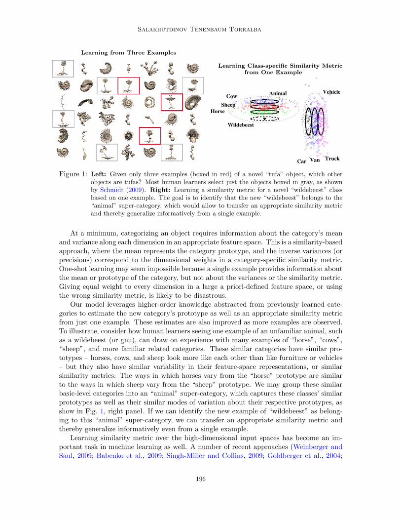
Figure 1: Left: Given only three examples (boxed in red) of a novel “tufa” object, which otherobjects are tufas? Most human learners select just the objects boxed in gray, as shownby Schmidt (2009). Right: Learning a similarity metric for a novel “wildebeest” classbased on one example. The goal is to identify that the new “wildebeest” belongs to the“animal” super-category, which would allow to transfer an appropriate similarity metricand thereby generalize informatively from a single example.

At a minimum, categorizing an object requires information about the category’s meanand variance along each dimension in an appropriate feature space. This is a similarity-basedapproach, where the mean represents the category prototype, and the inverse variances (orprecisions) correspond to the dimensional weights in a category-specific similarity metric.One-shot learning may seem impossible because a single example provides information aboutthe mean or prototype of the category, but not about the variances or the similarity metric.Giving equal weight to every dimension in a large a priori-defined feature space, or usingthe wrong similarity metric, is likely to be disastrous.

Our model leverages higher-order knowledge abstracted from previously learned cate-gories to estimate the new category’s prototype as well as an appropriate similarity metricfrom just one example. These estimates are also improved as more examples are observed.To illustrate, consider how human learners seeing one example of an unfamiliar animal, suchas a wildebeest (or gnu), can draw on experience with many examples of “horse”, “cows”,“sheep”, and more familiar related categories. These similar categories have similar pro-totypes – horses, cows, and sheep look more like each other than like furniture or vehicles– but they also have similar variability in their feature-space representations, or similarsimilarity metrics: The ways in which horses vary from the “horse” prototype are similarto the ways in which sheep vary from the “sheep” prototype. We may group these similarbasic-level categories into an “animal” super-category, which captures these classes’ similarprototypes as well as their similar modes of variation about their respective prototypes, asshow in Fig. 1, right panel. If we can identify the new example of “wildebeest” as belong-ing to this “animal” super-category, we can transfer an appropriate similarity metric andthereby generalize informatively even from a single example.

Learning similarity metric over the high-dimensional input spaces has become an im-portant task in machine learning as well. A number of recent approaches (Weinberger andSaul, 2009; Babenko et al., 2009; Singh-Miller and Collins, 2009; Goldberger et al., 2004;

196

One-Shot Learning

Salakhutdinov and Hinton, 2007; Chopra et al., 2005) have demonstrated that learning aclass-specific similarity metric can provide some insights into how high-dimensional datais organized and it can significantly improve the performance of algorithms like K-nearestneighbours that are based on computing distances. Most this work, however, focused onlearning similarity metrics when many labeled examples are available, and did not attemptto address the one-shot learning problem.

Although inspired by human learning, our approach is intended to be broadly useful formachine classification and AI tasks. To equip a robot with human-like object categorizationabilities, we must be able to learn tens of thousands of different categories, building on (andnot disrupting) representations of old ones (Bart and Ullman, 2005; Biederman, 1995). Inthese settings, learning from one or a few labeled examples and performing efficient inferencewill be crucial. Our method is designed to scale up in precisely these ways: a nonparametricprior allows new categories to be formed at any time in either supervised or unsupervisedmodes, and conjugate distributions allow most parameters to be integrated out analyticallyfor very fast inference.

2. Related Prior WorkHierarchical Bayesian models have previously been proposed (Kemp et al. (2006); Helleret al. (2009)) to describe how people learn to learn categories from one or a few examples, orlearn similarity metrics, but these approaches were not focused on machine learning settings– large-scale problems with many categories and high-dimensional natural image data. Alarge class of models based on hierarchical Dirichlet processes (Teh et al. (2006)) have alsobeen used for transfer learning (Sudderth et al. (2008); Canini and Griffiths (2009)). Thereare two key difference: First, HDPs typically assume a fixed hierarchy of classes for sharingparameters, while we learn the hierarchy in an unsupervised fashion. Second, HDPs aretypically given many examples for each category rather than the one-shot learning cases weconsider here. Recently introduced nested Dirichlet processes can also be used for transferlearning (Rodriguez and Vuppala (2009); Rodriguez et al. (2008)). However, this workassumes a fixed number of classes (or groups) and did not attempt to address one-shotlearning problem. A recent hierarchical model of Adams et al. (2011) could also be usedfor transfer learning tasks. However, this model does not learn hierarchical priors overcovariances, which is crucial for transferring an appropriate similarity metric to new basic-level categories in order to support learning from few examples. These recently introducedmodels are complementary to our approach, and can be combined productively, althoughwe leave that as a subject for future work.

There are several related approaches in the computer vision community. A hierarchicaltopic model for image features (Bart et al. (2008); Sivic et al. (2008)) can discover visualtaxonomies in an unsupervised fashion from large datasets but was not designed for one-shot learning of new categories. Perhaps closest to our work, Fei-Fei et al. (2006) also gavea hierarchical Bayesian model for visual categories with a prior on the parameters of newcategories that was induced from other categories. However, they learned a single priorshared across all categories and the prior was learned only from three categories, chosen byhand.

More generally, our goal contrasts with and complements that of computer vision effortson one-shot learning. We have attempted to minimize any tuning of our approach to

197

Salakhutdinov Tenenbaum Torralba

...

Cow Horse Sheep Truck Car

Animal VehicleLevel 1{µc, τ c}

Level 2

{µk, τk, αk}

Level 3{τ0, α0}

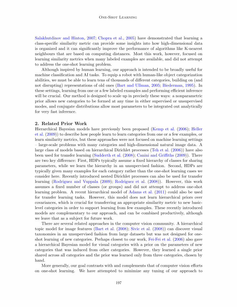
• For each super-category k = 1, ..,∞:

draw θ2 using Eq. 4.

• For each basic category ck = 1, ..,∞,placed under each super-category k:

draw θ1 using Eq. 2.

• For each observation n = 1, ..., N

draw zn ∼ nCRP(γ)draw xn ∼ N (xn|θ1, zn) using Eq. 1

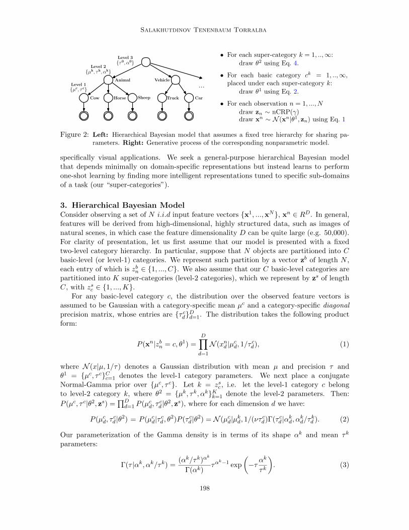
Figure 2: Left: Hierarchical Bayesian model that assumes a fixed tree hierarchy for sharing pa-rameters. Right: Generative process of the corresponding nonparametric model.

specifically visual applications. We seek a general-purpose hierarchical Bayesian modelthat depends minimally on domain-specific representations but instead learns to performone-shot learning by finding more intelligent representations tuned to specific sub-domainsof a task (our “super-categories”).

3. Hierarchical Bayesian ModelConsider observing a set of N i.i.d input feature vectors {x1, ...,xN}, xn ∈ RD. In general,features will be derived from high-dimensional, highly structured data, such as images ofnatural scenes, in which case the feature dimensionality D can be quite large (e.g. 50,000).For clarity of presentation, let us first assume that our model is presented with a fixedtwo-level category hierarchy. In particular, suppose that N objects are partitioned into Cbasic-level (or level-1) categories. We represent such partition by a vector zb of length N ,each entry of which is zbn ∈ {1, ..., C}. We also assume that our C basic-level categories arepartitioned into K super-categories (level-2 categories), which we represent by zs of lengthC, with zsc ∈ {1, ...,K}.

For any basic-level category c, the distribution over the observed feature vectors isassumed to be Gaussian with a category-specific mean µc and a category-specific diagonalprecision matrix, whose entries are {τ cd}Dd=1. The distribution takes the following productform:

P (xn|zbn = c, θ1) =D∏d=1

N (xnd |µcd, 1/τ cd), (1)

where N (x|µ, 1/τ) denotes a Gaussian distribution with mean µ and precision τ andθ1 = {µc, τ c}Cc=1 denotes the level-1 category parameters. We next place a conjugateNormal-Gamma prior over {µc, τ c}. Let k = zsc , i.e. let the level-1 category c belongto level-2 category k, where θ2 = {µk, τk, αk}Kk=1 denote the level-2 parameters. Then:

P (µc, τ c|θ2, zs) =∏Dd=1 P (µcd, τ

cd |θ2, zs), where for each dimension d we have:

P (µcd, τcd |θ2) = P (µcd|τ cd , θ2)P (τ cd |θ2) = N (µcd|µkd, 1/(ντ cd)Γ(τ cd |αkd, αkd/τkd ). (2)

Our parameterization of the Gamma density is in terms of its shape αk and mean τk

parameters:

Γ(τ |αk, αk/τk) =(αk/τk)α

k

Γ(αk)τα

k−1 exp

(−τ α

k

τk

). (3)

198

One-Shot Learning

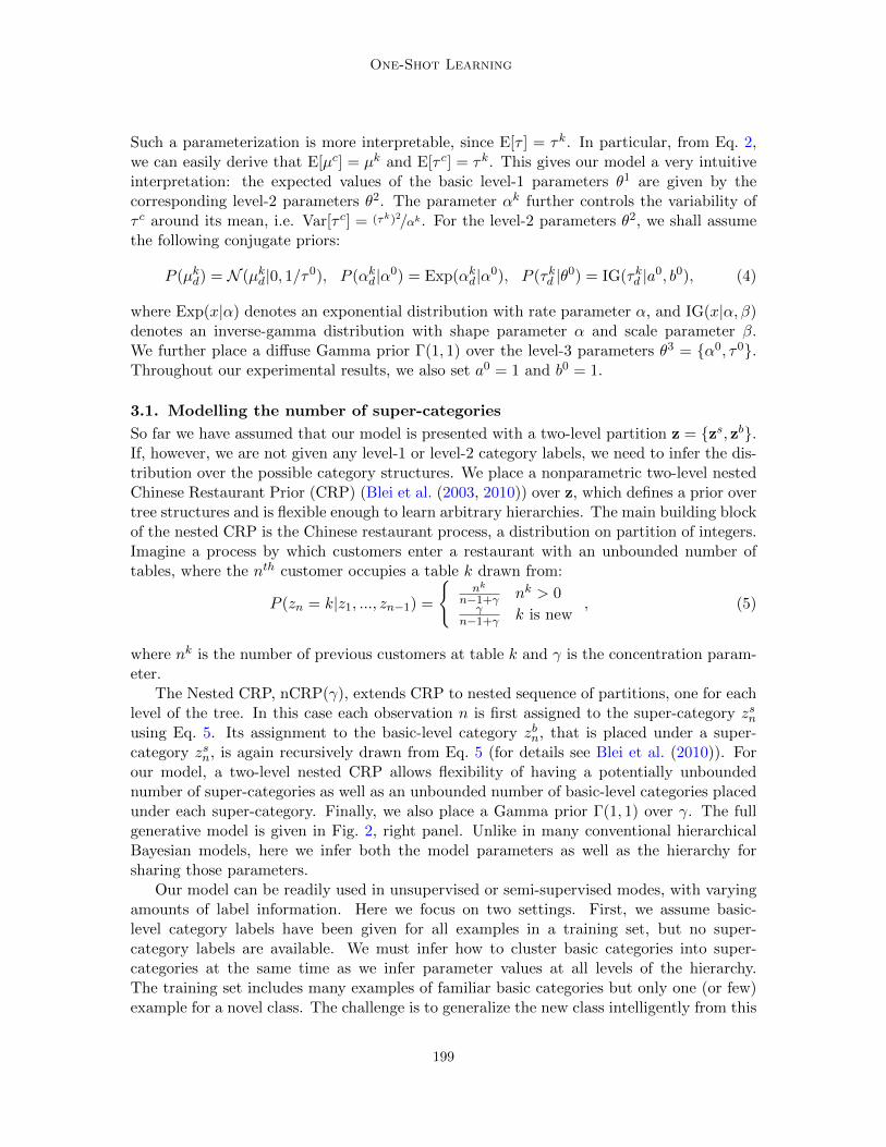
Such a parameterization is more interpretable, since E[τ ] = τk. In particular, from Eq. 2,we can easily derive that E[µc] = µk and E[τ c] = τk. This gives our model a very intuitiveinterpretation: the expected values of the basic level-1 parameters θ1 are given by thecorresponding level-2 parameters θ2. The parameter αk further controls the variability ofτ c around its mean, i.e. Var[τ c] = (τk)2/αk. For the level-2 parameters θ2, we shall assumethe following conjugate priors:

P (µkd) = N (µkd|0, 1/τ0), P (αkd|α0) = Exp(αkd|α0), P (τkd |θ0) = IG(τkd |a0, b0), (4)

where Exp(x|α) denotes an exponential distribution with rate parameter α, and IG(x|α, β)denotes an inverse-gamma distribution with shape parameter α and scale parameter β.We further place a diffuse Gamma prior Γ(1, 1) over the level-3 parameters θ3 = {α0, τ0}.Throughout our experimental results, we also set a0 = 1 and b0 = 1.

3.1. Modelling the number of super-categories

So far we have assumed that our model is presented with a two-level partition z = {zs, zb}.If, however, we are not given any level-1 or level-2 category labels, we need to infer the dis-tribution over the possible category structures. We place a nonparametric two-level nestedChinese Restaurant Prior (CRP) (Blei et al. (2003, 2010)) over z, which defines a prior overtree structures and is flexible enough to learn arbitrary hierarchies. The main building blockof the nested CRP is the Chinese restaurant process, a distribution on partition of integers.Imagine a process by which customers enter a restaurant with an unbounded number oftables, where the nth customer occupies a table k drawn from:

P (zn = k|z1, ..., zn−1) =

{nk

n−1+γ nk > 0γ

n−1+γ k is new, (5)

where nk is the number of previous customers at table k and γ is the concentration param-eter.

The Nested CRP, nCRP(γ), extends CRP to nested sequence of partitions, one for eachlevel of the tree. In this case each observation n is first assigned to the super-category zsnusing Eq. 5. Its assignment to the basic-level category zbn, that is placed under a super-category zsn, is again recursively drawn from Eq. 5 (for details see Blei et al. (2010)). Forour model, a two-level nested CRP allows flexibility of having a potentially unboundednumber of super-categories as well as an unbounded number of basic-level categories placedunder each super-category. Finally, we also place a Gamma prior Γ(1, 1) over γ. The fullgenerative model is given in Fig. 2, right panel. Unlike in many conventional hierarchicalBayesian models, here we infer both the model parameters as well as the hierarchy forsharing those parameters.

Our model can be readily used in unsupervised or semi-supervised modes, with varyingamounts of label information. Here we focus on two settings. First, we assume basic-level category labels have been given for all examples in a training set, but no super-category labels are available. We must infer how to cluster basic categories into super-categories at the same time as we infer parameter values at all levels of the hierarchy.The training set includes many examples of familiar basic categories but only one (or few)example for a novel class. The challenge is to generalize the new class intelligently from this

199

Salakhutdinov Tenenbaum Torralba

one example by inferring which super-category the new class comes from and exploitingthat super-category’s implied priors to estimate the new class’s prototype and similaritymetric most accurately. This training regime reflects natural language acquisition, wherespontaneous category labeling is frequent, almost all spontaneous labeling is at the basiclevel (Rosch et al., 1976) yet children’s generalizations are sensitive to higher superordinatestructure (Mandler, 2004), and where new basic-level categories are typically learned withhigh accuracy from just one or a few labeled examples. Second, we consider a similar labeledtraining set but now the test set consists of many unlabeled examples from an unknownnumber of basic-level classes – including both familiar and novel classes. This reflects theproblem of “unsupervised category learning” a child or robot faces in discovering when theyhave encountered novel categories, and how to break up new instances into categories inan intelligent way that exploits knowledge abstracted from a hierarchy of more familiarcategories.

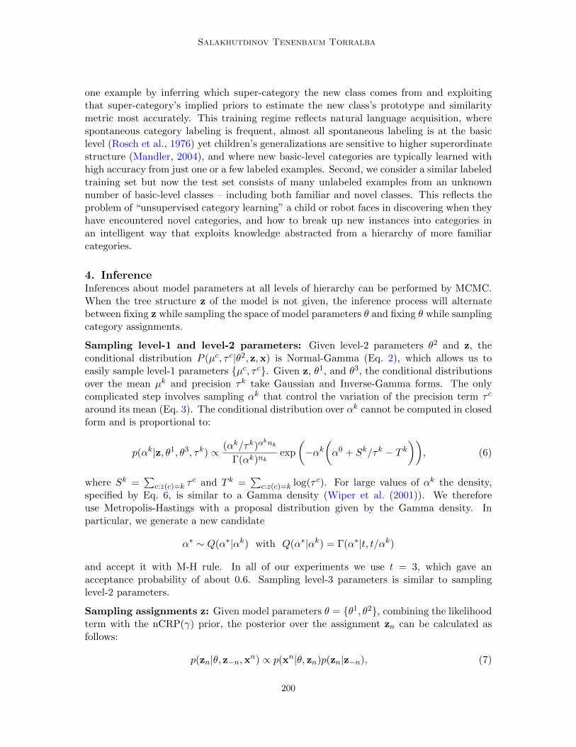
4. InferenceInferences about model parameters at all levels of hierarchy can be performed by MCMC.When the tree structure z of the model is not given, the inference process will alternatebetween fixing z while sampling the space of model parameters θ and fixing θ while samplingcategory assignments.

Sampling level-1 and level-2 parameters: Given level-2 parameters θ2 and z, theconditional distribution P (µc, τ c|θ2, z,x) is Normal-Gamma (Eq. 2), which allows us toeasily sample level-1 parameters {µc, τ c}. Given z, θ1, and θ3, the conditional distributionsover the mean µk and precision τk take Gaussian and Inverse-Gamma forms. The onlycomplicated step involves sampling αk that control the variation of the precision term τ c

around its mean (Eq. 3). The conditional distribution over αk cannot be computed in closedform and is proportional to:

p(αk|z, θ1, θ3, τk) ∝ (αk/τk)αknk

Γ(αk)nkexp

(−αk

(α0 + Sk/τk − T k

)), (6)

where Sk =∑

c:z(c)=k τc and T k =

∑c:z(c)=k log(τ c). For large values of αk the density,

specified by Eq. 6, is similar to a Gamma density (Wiper et al. (2001)). We thereforeuse Metropolis-Hastings with a proposal distribution given by the Gamma density. Inparticular, we generate a new candidate

α∗ ∼ Q(α∗|αk) with Q(α∗|αk) = Γ(α∗|t, t/αk)

and accept it with M-H rule. In all of our experiments we use t = 3, which gave anacceptance probability of about 0.6. Sampling level-3 parameters is similar to samplinglevel-2 parameters.

Sampling assignments z: Given model parameters θ = {θ1, θ2}, combining the likelihoodterm with the nCRP(γ) prior, the posterior over the assignment zn can be calculated asfollows:

p(zn|θ, z−n,xn) ∝ p(xn|θ, zn)p(zn|z−n), (7)

200

One-Shot Learning

where z−n denotes variables z for all observations other than n. We can further exploitthe conjugacy in our hierarchical model when computing the probability of creating a newbasic-level category. Using the fact that Normal-Gamma prior p(µc, τ c) is the conjugateprior of a normal distribution, we can easily compute the following marginal likelihood:

p(xn|θ2, zn) =

∫µc,τc

p(xn, µc, τ c|θ2, zn) =

∫µc,τc

p(xn|µc, τ c)p(µc, τ c|θ2, zn).

Integrating out basic-level parameters θ1 lets us more efficiently sample over the tree struc-tures1. When computing the probability of placing xn under a newly created super-category,its parameters are sampled from the prior.

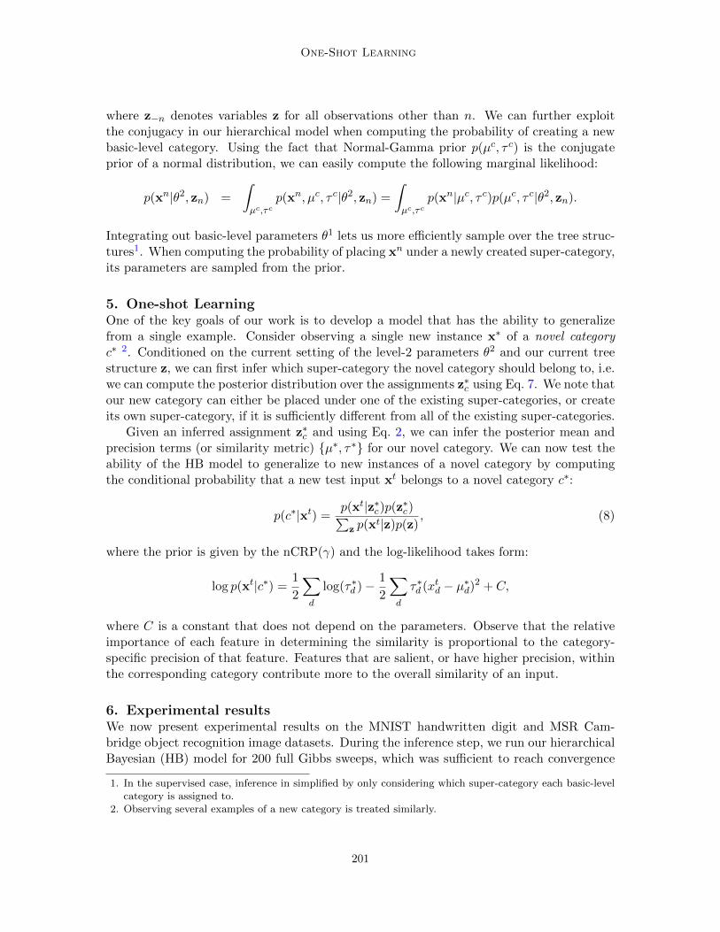
5. One-shot LearningOne of the key goals of our work is to develop a model that has the ability to generalizefrom a single example. Consider observing a single new instance x∗ of a novel categoryc∗ 2. Conditioned on the current setting of the level-2 parameters θ2 and our current treestructure z, we can first infer which super-category the novel category should belong to, i.e.we can compute the posterior distribution over the assignments z∗c using Eq. 7. We note thatour new category can either be placed under one of the existing super-categories, or createits own super-category, if it is sufficiently different from all of the existing super-categories.

Given an inferred assignment z∗c and using Eq. 2, we can infer the posterior mean andprecision terms (or similarity metric) {µ∗, τ∗} for our novel category. We can now test theability of the HB model to generalize to new instances of a novel category by computingthe conditional probability that a new test input xt belongs to a novel category c∗:

p(c∗|xt) =p(xt|z∗c)p(z∗c)∑z p(x

t|z)p(z), (8)

where the prior is given by the nCRP(γ) and the log-likelihood takes form:

log p(xt|c∗) =1

2

∑d

log(τ∗d )− 1

2

∑d

τ∗d (xtd − µ∗d)2 + C,

where C is a constant that does not depend on the parameters. Observe that the relativeimportance of each feature in determining the similarity is proportional to the category-specific precision of that feature. Features that are salient, or have higher precision, withinthe corresponding category contribute more to the overall similarity of an input.

6. Experimental resultsWe now present experimental results on the MNIST handwritten digit and MSR Cam-bridge object recognition image datasets. During the inference step, we run our hierarchicalBayesian (HB) model for 200 full Gibbs sweeps, which was sufficient to reach convergence

1. In the supervised case, inference in simplified by only considering which super-category each basic-levelcategory is assigned to.

2. Observing several examples of a new category is treated similarly.

201

Salakhutdinov Tenenbaum Torralba

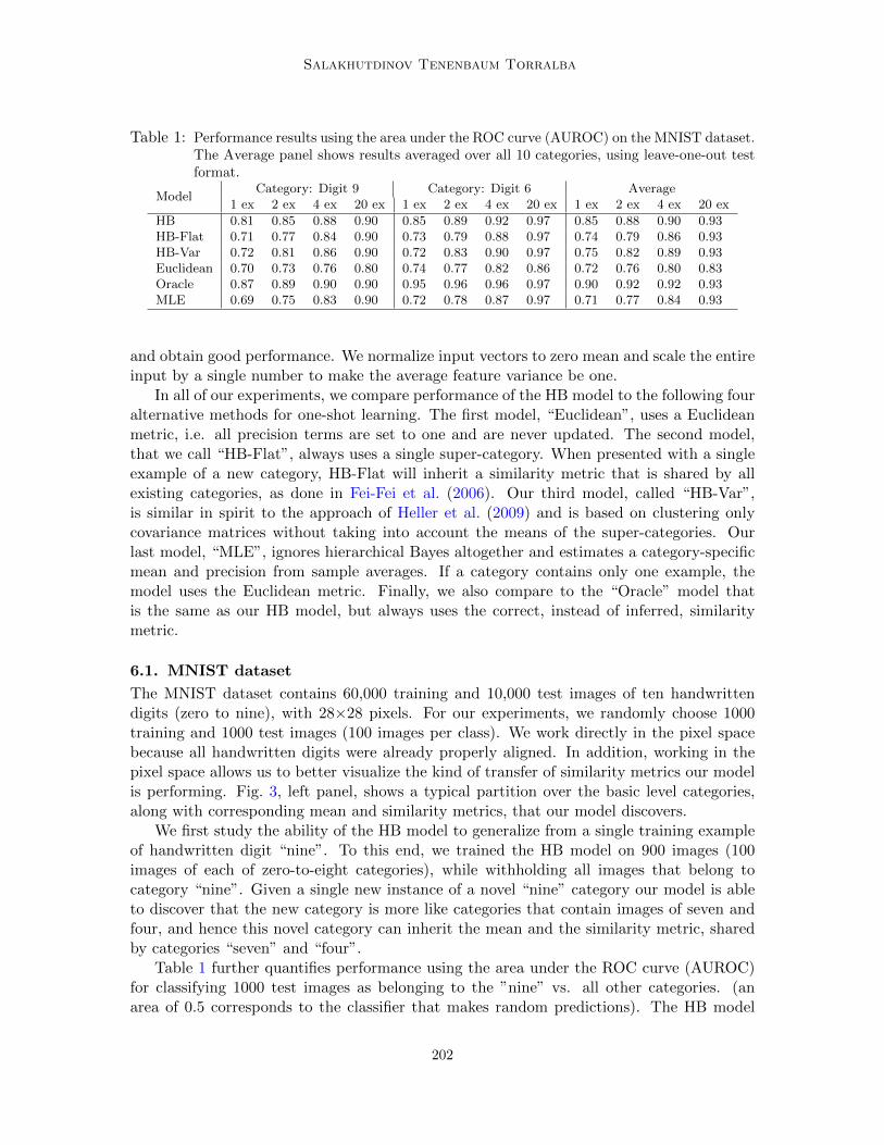
Table 1: Performance results using the area under the ROC curve (AUROC) on the MNIST dataset.The Average panel shows results averaged over all 10 categories, using leave-one-out testformat.

ModelCategory: Digit 9 Category: Digit 6 Average

1 ex 2 ex 4 ex 20 ex 1 ex 2 ex 4 ex 20 ex 1 ex 2 ex 4 ex 20 ex

HB 0.81 0.85 0.88 0.90 0.85 0.89 0.92 0.97 0.85 0.88 0.90 0.93HB-Flat 0.71 0.77 0.84 0.90 0.73 0.79 0.88 0.97 0.74 0.79 0.86 0.93HB-Var 0.72 0.81 0.86 0.90 0.72 0.83 0.90 0.97 0.75 0.82 0.89 0.93Euclidean 0.70 0.73 0.76 0.80 0.74 0.77 0.82 0.86 0.72 0.76 0.80 0.83Oracle 0.87 0.89 0.90 0.90 0.95 0.96 0.96 0.97 0.90 0.92 0.92 0.93MLE 0.69 0.75 0.83 0.90 0.72 0.78 0.87 0.97 0.71 0.77 0.84 0.93

and obtain good performance. We normalize input vectors to zero mean and scale the entireinput by a single number to make the average feature variance be one.

In all of our experiments, we compare performance of the HB model to the following fouralternative methods for one-shot learning. The first model, “Euclidean”, uses a Euclideanmetric, i.e. all precision terms are set to one and are never updated. The second model,that we call “HB-Flat”, always uses a single super-category. When presented with a singleexample of a new category, HB-Flat will inherit a similarity metric that is shared by allexisting categories, as done in Fei-Fei et al. (2006). Our third model, called “HB-Var”,is similar in spirit to the approach of Heller et al. (2009) and is based on clustering onlycovariance matrices without taking into account the means of the super-categories. Ourlast model, “MLE”, ignores hierarchical Bayes altogether and estimates a category-specificmean and precision from sample averages. If a category contains only one example, themodel uses the Euclidean metric. Finally, we also compare to the “Oracle” model thatis the same as our HB model, but always uses the correct, instead of inferred, similaritymetric.

6.1. MNIST dataset

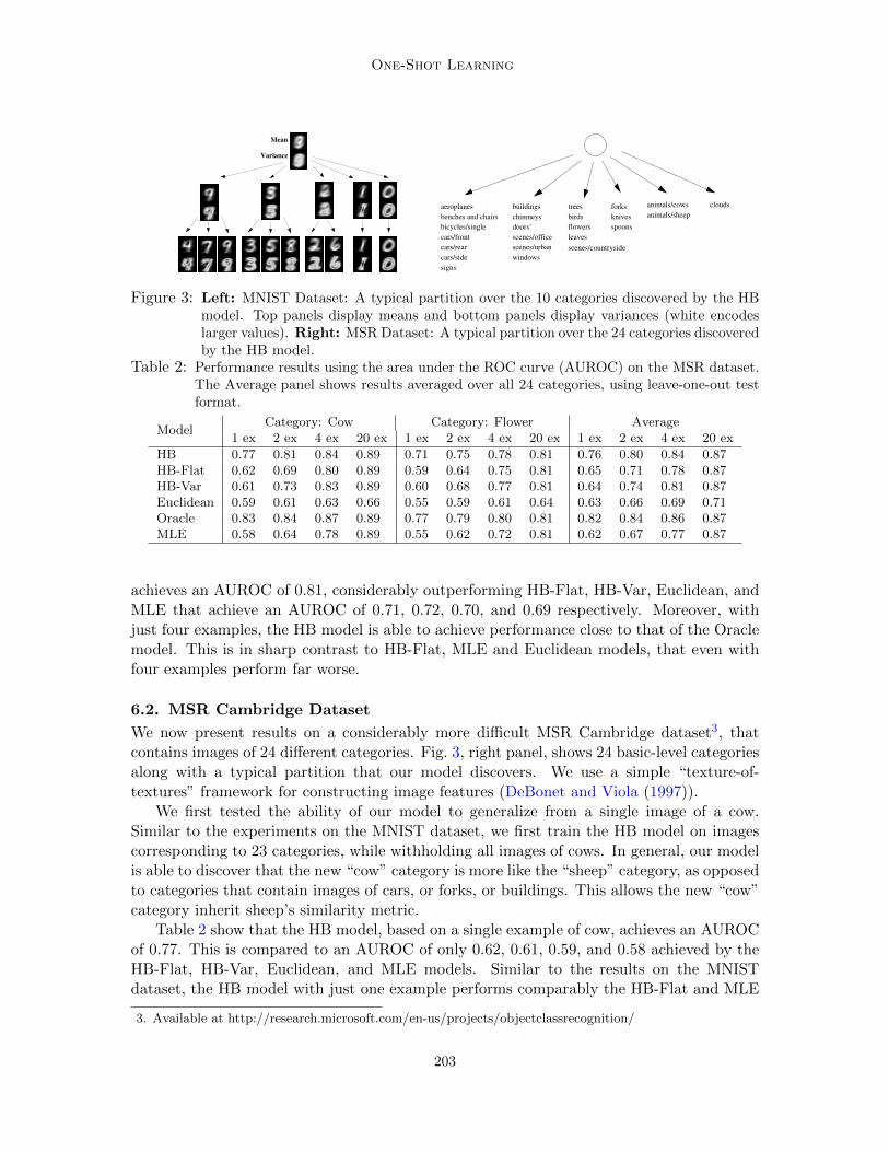
The MNIST dataset contains 60,000 training and 10,000 test images of ten handwrittendigits (zero to nine), with 28×28 pixels. For our experiments, we randomly choose 1000training and 1000 test images (100 images per class). We work directly in the pixel spacebecause all handwritten digits were already properly aligned. In addition, working in thepixel space allows us to better visualize the kind of transfer of similarity metrics our modelis performing. Fig. 3, left panel, shows a typical partition over the basic level categories,along with corresponding mean and similarity metrics, that our model discovers.

We first study the ability of the HB model to generalize from a single training exampleof handwritten digit “nine”. To this end, we trained the HB model on 900 images (100images of each of zero-to-eight categories), while withholding all images that belong tocategory “nine”. Given a single new instance of a novel “nine” category our model is ableto discover that the new category is more like categories that contain images of seven andfour, and hence this novel category can inherit the mean and the similarity metric, sharedby categories “seven” and “four”.

Table 1 further quantifies performance using the area under the ROC curve (AUROC)for classifying 1000 test images as belonging to the ”nine” vs. all other categories. (anarea of 0.5 corresponds to the classifier that makes random predictions). The HB model

202

One-Shot Learning

Mean

Variance

aeroplanes

benches and chairs

bicycles/single

cars/front

cars/rear

cars/side

signs

buildings

chimneys

doors’

scenes/office

scenes/urban

windows

cloudsforks

knives

spoons

trees

birds

flowers

leaves

animals/cows

animals/sheep

scenes/countryside

Figure 3: Left: MNIST Dataset: A typical partition over the 10 categories discovered by the HBmodel. Top panels display means and bottom panels display variances (white encodeslarger values). Right: MSR Dataset: A typical partition over the 24 categories discoveredby the HB model.

Table 2: Performance results using the area under the ROC curve (AUROC) on the MSR dataset.The Average panel shows results averaged over all 24 categories, using leave-one-out testformat.

ModelCategory: Cow Category: Flower Average

1 ex 2 ex 4 ex 20 ex 1 ex 2 ex 4 ex 20 ex 1 ex 2 ex 4 ex 20 ex

HB 0.77 0.81 0.84 0.89 0.71 0.75 0.78 0.81 0.76 0.80 0.84 0.87HB-Flat 0.62 0.69 0.80 0.89 0.59 0.64 0.75 0.81 0.65 0.71 0.78 0.87HB-Var 0.61 0.73 0.83 0.89 0.60 0.68 0.77 0.81 0.64 0.74 0.81 0.87Euclidean 0.59 0.61 0.63 0.66 0.55 0.59 0.61 0.64 0.63 0.66 0.69 0.71Oracle 0.83 0.84 0.87 0.89 0.77 0.79 0.80 0.81 0.82 0.84 0.86 0.87MLE 0.58 0.64 0.78 0.89 0.55 0.62 0.72 0.81 0.62 0.67 0.77 0.87

achieves an AUROC of 0.81, considerably outperforming HB-Flat, HB-Var, Euclidean, andMLE that achieve an AUROC of 0.71, 0.72, 0.70, and 0.69 respectively. Moreover, withjust four examples, the HB model is able to achieve performance close to that of the Oraclemodel. This is in sharp contrast to HB-Flat, MLE and Euclidean models, that even withfour examples perform far worse.

6.2. MSR Cambridge Dataset

We now present results on a considerably more difficult MSR Cambridge dataset3, thatcontains images of 24 different categories. Fig. 3, right panel, shows 24 basic-level categoriesalong with a typical partition that our model discovers. We use a simple “texture-of-textures” framework for constructing image features (DeBonet and Viola (1997)).

We first tested the ability of our model to generalize from a single image of a cow.Similar to the experiments on the MNIST dataset, we first train the HB model on imagescorresponding to 23 categories, while withholding all images of cows. In general, our modelis able to discover that the new “cow” category is more like the “sheep” category, as opposedto categories that contain images of cars, or forks, or buildings. This allows the new “cow”category inherit sheep’s similarity metric.

Table 2 show that the HB model, based on a single example of cow, achieves an AUROCof 0.77. This is compared to an AUROC of only 0.62, 0.61, 0.59, and 0.58 achieved by theHB-Flat, HB-Var, Euclidean, and MLE models. Similar to the results on the MNISTdataset, the HB model with just one example performs comparably the HB-Flat and MLE

3. Available at http://research.microsoft.com/en-us/projects/objectclassrecognition/

203

Salakhutdinov Tenenbaum Torralba

EuclideanQuery

Hierarchical Bayes

Query Euclidean

Hierarchical Bayes

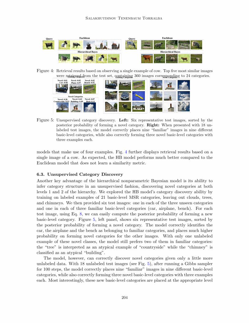
Figure 4: Retrieval results based on observing a single example of cow. Top five most similar imageswere retrieved from the test set, containing 360 images corresponding to 24 categories.

20 40 60 80 100 120 140 160 180 200

20

40

60

80

100

120

140

Existing Categories Existing Categories Novel Categories

Car: 0.99 Plane: 0.97

Novel: 0.02Novel: 0.01 Novel: 0.02Bench: 0.92

Countryside: 0.53 Building: 0.49 Bird: 0.11

Novel Categories

Novel: 0.28 Novel: 0.42 Novel: 0.87

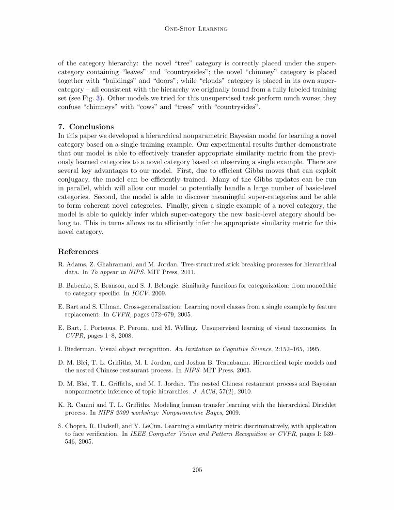
Figure 5: Unsupervised category discovery. Left: Six representative test images, sorted by theposterior probability of forming a novel category. Right: When presented with 18 un-labeled test images, the model correctly places nine “familiar” images in nine differentbasic-level categories, while also correctly forming three novel basic-level categories withthree examples each.

models that make use of four examples. Fig. 4 further displays retrieval results based on asingle image of a cow. As expected, the HB model performs much better compared to theEuclidean model that does not learn a similarity metric.

6.3. Unsupervised Category Discovery

Another key advantage of the hierarchical nonparametric Bayesian model is its ability toinfer category structure in an unsupervised fashion, discovering novel categories at bothlevels 1 and 2 of the hierarchy. We explored the HB model’s category discovery ability bytraining on labeled examples of 21 basic-level MSR categories, leaving out clouds, trees,and chimneys. We then provided six test images: one in each of the three unseen categoriesand one in each of three familiar basic-level categories (car, airplane, bench). For eachtest image, using Eq. 8, we can easily compute the posterior probability of forming a newbasic-level category. Figure 5, left panel, shows six representative test images, sorted bythe posterior probability of forming a novel category. The model correctly identifies thecar, the airplane and the bench as belonging to familiar categories, and places much higherprobability on forming novel categories for the other images. With only one unlabeledexample of these novel classes, the model still prefers two of them in familiar categories:the “tree” is interpreted as an atypical example of “countryside” while the “chimney” isclassified as an atypical “building”.

The model, however, can correctly discover novel categories given only a little moreunlabeled data. With 18 unlabeled test images (see Fig. 5), after running a Gibbs samplerfor 100 steps, the model correctly places nine “familiar” images in nine different basic-levelcategories, while also correctly forming three novel basic-level categories with three exampleseach. Most interestingly, these new basic-level categories are placed at the appropriate level

204

One-Shot Learning

of the category hierarchy: the novel “tree” category is correctly placed under the super-category containing “leaves” and “countrysides”; the novel “chimney” category is placedtogether with “buildings” and “doors”; while “clouds” category is placed in its own super-category – all consistent with the hierarchy we originally found from a fully labeled trainingset (see Fig. 3). Other models we tried for this unsupervised task perform much worse; theyconfuse “chimneys” with “cows” and “trees” with “countrysides”.

7. ConclusionsIn this paper we developed a hierarchical nonparametric Bayesian model for learning a novelcategory based on a single training example. Our experimental results further demonstratethat our model is able to effectively transfer appropriate similarity metric from the previ-ously learned categories to a novel category based on observing a single example. There areseveral key advantages to our model. First, due to efficient Gibbs moves that can exploitconjugacy, the model can be efficiently trained. Many of the Gibbs updates can be runin parallel, which will allow our model to potentially handle a large number of basic-levelcategories. Second, the model is able to discover meaningful super-categories and be ableto form coherent novel categories. Finally, given a single example of a novel category, themodel is able to quickly infer which super-category the new basic-level ategory should be-long to. This in turns allows us to efficiently infer the appropriate similarity metric for thisnovel category.

References

R. Adams, Z. Ghahramani, and M. Jordan. Tree-structured stick breaking processes for hierarchicaldata. In To appear in NIPS. MIT Press, 2011.

B. Babenko, S. Branson, and S. J. Belongie. Similarity functions for categorization: from monolithicto category specific. In ICCV, 2009.

E. Bart and S. Ullman. Cross-generalization: Learning novel classes from a single example by featurereplacement. In CVPR, pages 672–679, 2005.

E. Bart, I. Porteous, P. Perona, and M. Welling. Unsupervised learning of visual taxonomies. InCVPR, pages 1–8, 2008.

I. Biederman. Visual object recognition. An Invitation to Cognitive Science, 2:152–165, 1995.

D. M. Blei, T. L. Griffiths, M. I. Jordan, and Joshua B. Tenenbaum. Hierarchical topic models andthe nested Chinese restaurant process. In NIPS. MIT Press, 2003.

D. M. Blei, T. L. Griffiths, and M. I. Jordan. The nested Chinese restaurant process and Bayesiannonparametric inference of topic hierarchies. J. ACM, 57(2), 2010.

K. R. Canini and T. L. Griffiths. Modeling human transfer learning with the hierarchical Dirichletprocess. In NIPS 2009 workshop: Nonparametric Bayes, 2009.

S. Chopra, R. Hadsell, and Y. LeCun. Learning a similarity metric discriminatively, with applicationto face verification. In IEEE Computer Vision and Pattern Recognition or CVPR, pages I: 539–546, 2005.

205

Salakhutdinov Tenenbaum Torralba

J. S. DeBonet and P. A. Viola. Structure driven image database retrieval. In Michael I. Jordan,Michael J. Kearns, and Sara A. Solla, editors, NIPS. The MIT Press, 1997.

Li Fei-Fei, R. Fergus, and P. Perona. One-shot learning of object categories. IEEE Trans. PatternAnalysis and Machine Intelligence, 28(4):594–611, April 2006.

J. Goldberger, S. T. Roweis, G. E. Hinton, and R. R. Salakhutdinov. Neighbourhood componentsanalysis. In Advances in Neural Information Processing Systems, 2004.

K. Heller, A. Sanborn, and N. Chater. Hierarchical learning of dimensional biases in human catego-rization. In NIPS, 2009.

C. Kemp, A. Perfors, and J. Tenenbaum. Learning overhypotheses with hierarchical Bayesian models.Developmental Science, 10(3):307–321, 2006.

J.M. Mandler. The foundations of mind: Origins of conceptual thought. Oxford University Press,USA, 2004.

A. Perfors and J.B. Tenenbaum. Learning to learn categories. In 31st Annual Conference of theCognitive Science Society, pages 136–141, 2009.

S. Pinker. How the Mind Works. W.W. Norton, 1999.

A. Rodriguez and R. Vuppala. Probabilistic classification using Bayesian nonparametric mixturemodels. Technical Report, 2009.

A. Rodriguez, D. Dunson, and A. Gelfand. The nested Dirichlet process. Journal of the AmericanStatistical Association, 103:1131–1144, 2008.

E. Rosch, C.B. Mervis, W.D. Gray, D.M. Johnson, and P. Boyes-Braem. Basic objects in naturalcategories* 1. Cognitive psychology, 8(3):382–439, 1976.

R. R. Salakhutdinov and G. E. Hinton. Learning a nonlinear embedding by preserving class neigh-bourhood structure. In Proceedings of the International Conference on Artificial Intelligence andStatistics, volume 11, 2007.

L. Schmidt. Meaning and compositionality as statistical induction of categories and constraints.Ph.D Thesis, Massachusetts Institute of Technology, 2009.

N. Singh-Miller and M. Collins. Learning label embeddings for nearest-neighbor multi-class classifi-cation with an application to speech recognition. In Advances in Neural Information ProcessingSystems. MIT Press, 2009.

J. Sivic, B. C. Russell, A. Zisserman, W. T. Freeman, and A. A. Efros. Unsupervised discovery ofvisual object class hierarchies. In CVPR, pages 1–8, 2008.

L.B. Smith, S.S. Jones, B. Landau, L. Gershkoff-Stowe, and L. Samuelson. Object name learningprovides on-the-job training for attention. Psychological Science, pages 13–19, 2002.

E. B. Sudderth, A. Torralba, W. T. Freeman, and A. S. Willsky. Describing visual scenes usingtransformed objects and parts. International Journal of Computer Vision, 77(1-3):291–330, 2008.

Y. W. Teh, M. I. Jordan, M. J. Beal, and D. M. Blei. Hierarchical Dirichlet processes. Journal ofthe American Statistical Association, 101(476):1566–1581, 2006.

206

One-Shot Learning

K. Q. Weinberger and L. K. Saul. Distance metric learning for large margin nearest neighborclassification. Journal of Machine Learning Research, 3, 2009.

M. Wiper, D. R. Insua, and F. Ruggeri. Mixtures of Gamma distributions with applications. Journalof Computational and Graphical Statistics, 10(3), September 2001.

F. Xu and J. B. Tenenbaum. Word learning as Bayesian inference. Psychological Review, 114(2),2007.

207