one-shot learning with memory-augmented neural networks · one-shot learning with memory-augmented...

One-shot Learning with Memory-Augmented Neural Networks

Adam Santoro [email protected]

Google DeepMind

Sergey Bartunov [email protected]

Google DeepMind, National Research University Higher School of Economics (HSE)

Matthew Botvinick [email protected] Wierstra [email protected] Lillicrap [email protected]

Google DeepMind

AbstractDespite recent breakthroughs in the applicationsof deep neural networks, one setting that presentsa persistent challenge is that of “one-shot learn-ing.” Traditional gradient-based networks requirea lot of data to learn, often through extensive it-erative training. When new data is encountered,the models must inefficiently relearn their param-eters to adequately incorporate the new informa-tion without catastrophic interference. Architec-tures with augmented memory capacities, such asNeural Turing Machines (NTMs), offer the abil-ity to quickly encode and retrieve new informa-tion, and hence can potentially obviate the down-sides of conventional models. Here, we demon-strate the ability of a memory-augmented neu-ral network to rapidly assimilate new data, andleverage this data to make accurate predictionsafter only a few samples. We also introduce anew method for accessing an external memorythat focuses on memory content, unlike previousmethods that additionally use memory location-based focusing mechanisms.

1. IntroductionThe current success of deep learning hinges on the abil-ity to apply gradient-based optimization to high-capacitymodels. This approach has achieved impressive results onmany large-scale supervised tasks with raw sensory input,such as image classification (He et al., 2015), speech recog-nition (Yu & Deng, 2012), and games (Mnih et al., 2015;Silver et al., 2016). Notably, performance in such tasks istypically evaluated after extensive, incremental training onlarge data sets. In contrast, many problems of interest re-

quire rapid inference from small quantities of data. In thelimit of “one-shot learning,” single observations should re-sult in abrupt shifts in behavior.

This kind of flexible adaptation is a celebrated aspect of hu-man learning (Jankowski et al., 2011), manifesting in set-tings ranging from motor control (Braun et al., 2009) to theacquisition of abstract concepts (Lake et al., 2015). Gener-ating novel behavior based on inference from a few scrapsof information – e.g., inferring the full range of applicabil-ity for a new word, heard in only one or two contexts – issomething that has remained stubbornly beyond the reachof contemporary machine intelligence. It appears to presenta particularly daunting challenge for deep learning. In sit-uations when only a few training examples are presentedone-by-one, a straightforward gradient-based solution is tocompletely re-learn the parameters from the data availableat the moment. Such a strategy is prone to poor learning,and/or catastrophic interference. In view of these hazards,non-parametric methods are often considered to be bettersuited.

However, previous work does suggest one potential strat-egy for attaining rapid learning from sparse data, andhinges on the notion of meta-learning (Thrun, 1998; Vi-lalta & Drissi, 2002). Although the term has been usedin numerous senses (Schmidhuber et al., 1997; Caruana,1997; Schweighofer & Doya, 2003; Brazdil et al., 2003),meta-learning generally refers to a scenario in which anagent learns at two levels, each associated with differenttime scales. Rapid learning occurs within a task, for ex-ample, when learning to accurately classify within a par-ticular dataset. This learning is guided by knowledgeaccrued more gradually across tasks, which captures theway in which task structure varies across target domains(Giraud-Carrier et al., 2004; Rendell et al., 1987; Thrun,1998). Given its two-tiered organization, this form of meta-

arX

iv:1

605.

0606

5v1

[cs

.LG

] 1

9 M

ay 2

016

One-shot learning with Memory-Augmented Neural Networks

learning is often described as “learning to learn.”

It has been proposed that neural networks with mem-ory capacities could prove quite capable of meta-learning(Hochreiter et al., 2001). These networks shift their biasthrough weight updates, but also modulate their output bylearning to rapidly cache representations in memory stores(Hochreiter & Schmidhuber, 1997). For example, LSTMstrained to meta-learn can quickly learn never-before-seenquadratic functions with a low number of data samples(Hochreiter et al., 2001).

Neural networks with a memory capacity provide a promis-ing approach to meta-learning in deep networks. However,the specific strategy of using the memory inherent in un-structured recurrent architectures is unlikely to extend tosettings where each new task requires significant amountsof new information to be rapidly encoded. A scalable so-lution has a few necessary requirements: First, informationmust be stored in memory in a representation that is bothstable (so that it can be reliably accessed when needed) andelement-wise addressable (so that relevant pieces of infor-mation can be accessed selectively). Second, the numberof parameters should not be tied to the size of the mem-ory. These two characteristics do not arise naturally withinstandard memory architectures, such as LSTMs. How-ever, recent architectures, such as Neural Turing Machines(NTMs) (Graves et al., 2014) and memory networks (We-ston et al., 2014), meet the requisite criteria. And so, in thispaper we revisit the meta-learning problem and setup fromthe perspective of a highly capable memory-augmentedneural network (MANN) (note: here on, the term MANNwill refer to the class of external-memory equipped net-works, and not other “internal” memory-based architec-tures, such as LSTMs).

We demonstrate that MANNs are capable of meta-learningin tasks that carry significant short- and long-term mem-ory demands. This manifests as successful classificationof never-before-seen Omniglot classes at human-like accu-racy after only a few presentations, and principled functionestimation based on a small number of samples. Addition-ally, we outline a memory access module that emphasizesmemory access by content, and not additionally on mem-ory location, as in original implementations of the NTM(Graves et al., 2014). Our approach combines the best oftwo worlds: the ability to slowly learn an abstract methodfor obtaining useful representations of raw data, via gra-dient descent, and the ability to rapidly bind never-before-seen information after a single presentation, via an externalmemory module. The combination supports robust meta-learning, extending the range of problems to which deeplearning can be effectively applied.

2. Meta-Learning Task MethodologyUsually, we try to choose parameters θ to minimize a learn-ing cost L across some dataset D. However, for meta-learning, we choose parameters to reduce the expectedlearning cost across a distribution of datasets p(D):

θ∗ = argminθED∼p(D)[L(D; θ)]. (1)

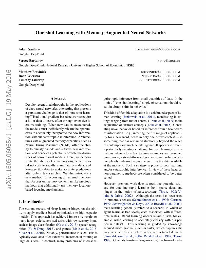
To accomplish this, proper task setup is critical (Hochre-iter et al., 2001). In our setup, a task, or episode, in-volves the presentation of some dataset D = {dt}Tt=1 ={(xt, yt)}Tt=1. For classification, yt is the class label foran image xt, and for regression, yt is the value of a hid-den function for a vector with real-valued elements xt, orsimply a real-valued number xt (here on, for consistency,xt will be used). In this setup, yt is both a target, andis presented as input along with xt, in a temporally off-set manner; that is, the network sees the input sequence(x1, null), (x2, y1), . . . , (xT , yT−1). And so, at time t thecorrect label for the previous data sample (yt−1) is pro-vided as input along with a new query xt (see Figure 1 (a)).The network is tasked to output the appropriate label forxt (i.e., yt) at the given timestep. Importantly, labels areshuffled from dataset-to-dataset. This prevents the networkfrom slowly learning sample-class bindings in its weights.Instead, it must learn to hold data samples in memory un-til the appropriate labels are presented at the next time-step, after which sample-class information can be boundand stored for later use (see Figure 1 (b)). Thus, for a givenepisode, ideal performance involves a random guess for thefirst presentation of a class (since the appropriate label cannot be inferred from previous episodes, due to label shuf-fling), and the use of memory to achieve perfect accuracythereafter. Ultimately, the system aims at modelling thepredictive distribution p(yt|xt, D1:t−1; θ), inducing a cor-responding loss at each time step.

This task structure incorporates exploitable meta-knowledge: a model that meta-learns would learn to binddata representations to their appropriate labels regardlessof the actual content of the data representation or label,and would employ a general scheme to map these boundrepresentations to appropriate classes or function valuesfor prediction.

3. Memory-Augmented Model3.1. Neural Turing Machines

The Neural Turing Machine is a fully differentiable imple-mentation of a MANN. It consists of a controller, such asa feed-forward network or LSTM, which interacts with anexternal memory module using a number of read and writeheads (Graves et al., 2014). Memory encoding and retrievalin a NTM external memory module is rapid, with vector


(a) Task setup (b) Network strategy

Figure 1. Task structure. (a) Omniglot images (or x-values for regression), xt, are presented with time-offset labels (or function values),yt−1, to prevent the network from simply mapping the class labels to the output. From episode to episode, the classes to be presentedin the episode, their associated labels, and the specific samples are all shuffled. (b) A successful strategy would involve the use of anexternal memory to store bound sample representation-class label information, which can then be retrieved at a later point for successfulclassification when a sample from an already-seen class is presented. Specifically, sample data xt from a particular time step should bebound to the appropriate class label yt, which is presented in the subsequent time step. Later, when a sample from this same class isseen, it should retrieve this bound information from the external memory to make a prediction. Backpropagated error signals from thisprediction step will then shape the weight updates from the earlier steps in order to promote this binding strategy.

representations being placed into or taken out of memorypotentially every time-step. This ability makes the NTMa perfect candidate for meta-learning and low-shot predic-tion, as it is capable of both long-term storage via slow up-dates of its weights, and short-term storage via its exter-nal memory module. Thus, if a NTM can learn a generalstrategy for the types of representations it should place intomemory and how it should later use these representationsfor predictions, then it may be able use its speed to makeaccurate predictions of data that it has only seen once.

The controllers employed in our model are are eitherLSTMs, or feed-forward networks. The controller inter-acts with an external memory module using read and writeheads, which act to retrieve representations from memoryor place them into memory, respectively. Given some in-put, xt, the controller produces a key, kt, which is theneither stored in a row of a memory matrix Mt, or used toretrieve a particular memory, i, from a row; i.e., Mt(i).When retrieving a memory, Mt is addressed using the co-sine similarity measure,

K(kt,Mt(i)

)=

kt ·Mt(i)

‖ kt ‖‖Mt(i) ‖, (2)

which is used to produce a read-weight vector, wrt , with

elements computed according to a softmax:

wrt (i)←exp(K(kt,Mt(i)

))∑j exp

(K(kt,Mt(j)

)) . (3)

A memory, rt, is retrieved using this weight vector:

rt ←∑i

wrt (i)Mt(i). (4)

This memory is used by the controller as the input to a clas-sifier, such as a softmax output layer, and as an additionalinput for the next controller state.

3.2. Least Recently Used Access

In previous instantiations of the NTM (Graves et al., 2014),memories were addressed by both content and location.Location-based addressing was used to promote iterativesteps, akin to running along a tape, as well as long-distancejumps across memory. This method was advantageous forsequence-based prediction tasks. However, this type of ac-cess is not optimal for tasks that emphasize a conjunctivecoding of information independent of sequence. As such,writing to memory in our model involves the use of a newlydesigned access module called the Least Recently UsedAccess (LRUA) module.

The LRUA module is a pure content-based memory writerthat writes memories to either the least used memory lo-cation or the most recently used memory location. Thismodule emphasizes accurate encoding of relevant (i.e., re-cent) information, and pure content-based retrieval. Newinformation is written into rarely-used locations, preserv-ing recently encoded information, or it is written to thelast used location, which can function as an update of thememory with newer, possibly more relevant information.The distinction between these two options is accomplishedwith an interpolation between the previous read weightsand weights scaled according to usage weights wu

t . Theseusage weights are updated at each time-step by decayingthe previous usage weights and adding the current read and


write weights:

wut ← γwu

t−1 +wrt +ww

t . (5)

Here, γ is a decay parameter and wrt is computed as in (3).

The least-used weights, wlut , for a given time-step can then

be computed using wut . First, we introduce the notation

m(v, n) to denote the nth smallest element of the vector v.Elements of wlu

t are set accordingly:

wlut (i) =

{0 if wut (i) > m(wu

t , n)1 if wut (i) ≤ m(wu

t , n), (6)

where n is set to equal the number of reads to memory.To obtain the write weights ww

t , a learnable sigmoid gateparameter is used to compute a convex combination of theprevious read weights and previous least-used weights:

wwt ← σ(α)wr

t−1 + (1− σ(α))wlut−1. (7)

Here, σ(·) is a sigmoid function, 11+e−x , and α is a scalar

gate parameter to interpolate between the weights. Priorto writing to memory, the least used memory location iscomputed from wu

t−1 and is set to zero. Writing to mem-ory then occurs in accordance with the computed vector ofwrite weights:

Mt(i)←Mt−1(i) + wwt (i)kt,∀i (8)

Thus, memories can be written into the zeroed memory slotor the previously used slot; if it is the latter, then the leastused memories simply get erased.

4. Experimental Results4.1. Data

Two sources of data were used: Omniglot, for classifica-tion, and sampled functions from a Gaussian process (GP)with fixed hyperparameters, for regression. The Omniglotdataset consists of over 1600 separate classes with only afew examples per class, aptly lending to it being called thetranspose of MNIST (Lake et al., 2015). To reduce therisk of overfitting, we performed data augmentation by ran-domly translating and rotating character images. We alsocreated new classes through 90◦, 180◦ and 270◦ rotationsof existing data. The training of all models was performedon the data of 1200 original classes (plus augmentations),with the rest of the 423 classes (plus augmentations) beingused for test experiments. In order to reduce the computa-tional time of our experiments we downscaled the imagesto 20× 20.

4.2. Omniglot Classification

We performed a number of iterations of the basic task de-scribed in Section 2. First, our MANN was trained using

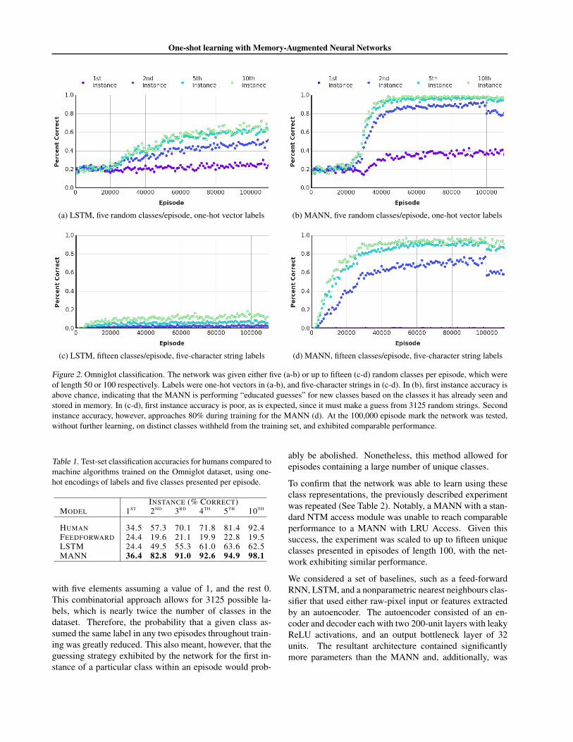
one-hot vector representations as class labels (Figure 2).After training on 100,000 episodes with five randomly cho-sen classes with randomly chosen labels, the network wasgiven a series of test episodes. In these episodes, no furtherlearning occurred, and the network was to predict the classlabels for never-before-seen classes pulled from a disjointtest set from within Omniglot. The network exhibited highclassification accuracy on just the second presentation of asample from a class within an episode (82.8%), reaching upto 94.9% accuracy by the fifth instance and 98.1% accuracyby the tenth.

For classification using one-hot vector representations, onerelevant baseline is human performance. Participants werefirst given instructions detailing the task: an image wouldappear, and they must choose an appropriate digit labelfrom the integers 1 through 5. Next, the image was pre-sented and they were to make an un-timed prediction asto its class label. The image then disappeared, and theywere given visual feedback as to their correctness, alongwith the correct label. The correct label was presented re-gardless of the accuracy of their prediction, allowing themto further reinforce correct decisions. After a short delayof two seconds, a new image appeared and they repeatedthe prediction process. The participants were not permittedto view previous images, or to use a scratch pad for ex-ternalization of memory. Performance of the MANN sur-passed that of a human on each instance. Interestingly, theMANN displayed better than random guessing on the firstinstance within a class. Seemingly, it employed a strategyof educated guessing; if a particular sample produced a keythat was a poor match to any of the bindings stored in ex-ternal memory, then the network was less likely to choosethe class labels associated with these stored bindings, andhence increased its probability of correctly guessing thisnew class on the first instance. A similar strategy was re-ported qualitatively by the human participants. We wereunable to accumulate an appreciable amount of data fromparticipants on the fifteen class case, as it proved much toodifficult and highly demotivating. For all intents and pur-poses, as the number of classes scale to fifteen and beyond,this type of binding surpasses human working memory ca-pacity, which is limited to storing only a handful of arbi-trary bindings (Cowan, 2010).

Since learning the weights of a classifier using large one-hot vectors becomes increasingly difficult with scale, a dif-ferent approach for labeling classes was employed so thatthe number of classes presented in a given episode could bearbitrarily increased. These new labels consisted of stringsof five characters, with each character assuming one of fivepossible values. Characters for each label were uniformlysampled from the set {‘a’, ‘b’, ‘c’, ‘d’, ‘e’}, producing ran-dom strings such as ‘ecdba’. Strings were represented asconcatenated one-hot vectors, and hence were of length 25


(a) LSTM, five random classes/episode, one-hot vector labels (b) MANN, five random classes/episode, one-hot vector labels

(c) LSTM, fifteen classes/episode, five-character string labels (d) MANN, fifteen classes/episode, five-character string labels

Figure 2. Omniglot classification. The network was given either five (a-b) or up to fifteen (c-d) random classes per episode, which wereof length 50 or 100 respectively. Labels were one-hot vectors in (a-b), and five-character strings in (c-d). In (b), first instance accuracy isabove chance, indicating that the MANN is performing “educated guesses” for new classes based on the classes it has already seen andstored in memory. In (c-d), first instance accuracy is poor, as is expected, since it must make a guess from 3125 random strings. Secondinstance accuracy, however, approaches 80% during training for the MANN (d). At the 100,000 episode mark the network was tested,without further learning, on distinct classes withheld from the training set, and exhibited comparable performance.

Table 1. Test-set classification accuracies for humans compared tomachine algorithms trained on the Omniglot dataset, using one-hot encodings of labels and five classes presented per episode.

INSTANCE (% CORRECT)MODEL 1ST 2ND 3RD 4TH 5TH 10TH

HUMAN 34.5 57.3 70.1 71.8 81.4 92.4FEEDFORWARD 24.4 19.6 21.1 19.9 22.8 19.5LSTM 24.4 49.5 55.3 61.0 63.6 62.5MANN 36.4 82.8 91.0 92.6 94.9 98.1

with five elements assuming a value of 1, and the rest 0.This combinatorial approach allows for 3125 possible la-bels, which is nearly twice the number of classes in thedataset. Therefore, the probability that a given class as-sumed the same label in any two episodes throughout train-ing was greatly reduced. This also meant, however, that theguessing strategy exhibited by the network for the first in-stance of a particular class within an episode would prob-

ably be abolished. Nonetheless, this method allowed forepisodes containing a large number of unique classes.

To confirm that the network was able to learn using theseclass representations, the previously described experimentwas repeated (See Table 2). Notably, a MANN with a stan-dard NTM access module was unable to reach comparableperformance to a MANN with LRU Access. Given thissuccess, the experiment was scaled to up to fifteen uniqueclasses presented in episodes of length 100, with the net-work exhibiting similar performance.

We considered a set of baselines, such as a feed-forwardRNN, LSTM, and a nonparametric nearest neighbours clas-sifier that used either raw-pixel input or features extractedby an autoencoder. The autoencoder consisted of an en-coder and decoder each with two 200-unit layers with leakyReLU activations, and an output bottleneck layer of 32units. The resultant architecture contained significantlymore parameters than the MANN and, additionally, was


allowed to train on three times as much augmented data.The highest accuracies from our experiments are reported,which were achieved using a single nearest neighbour forprediction and features from the output bottleneck layer ofthe autoencoder. Importantly, the nearest neighbour classi-fier had an unlimited amount of memory, and could auto-matically store and retrieve all previously seen examples.This provided the kNN with an distinct advantage, evenwhen raw pixels were used as input representations. Al-though using rich features extracted by the autoencoder fur-ther improved performance, the kNN baseline was clearlyoutperformed by the MANN.

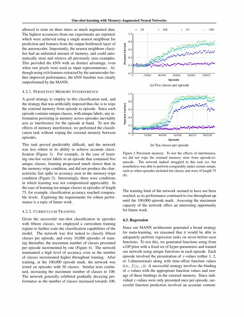
4.2.1. PERSISTENT MEMORY INTERFERENCE

A good strategy to employ in this classification task, andthe strategy that was artificially imposed thus-far, is to wipethe external memory from episode to episode. Since eachepisode contains unique classes, with unique labels, any in-formation persisting in memory across episodes inevitablyacts as interference for the episode at hand. To test theeffects of memory interference, we performed the classifi-cation task without wiping the external memory betweenepisodes.

This task proved predictably difficult, and the networkwas less robust in its ability to achieve accurate classi-fication (Figure 3). For example, in the case of learn-ing one-hot vector labels in an episode that contained fiveunique classes, learning progressed much slower than inthe memory-wipe condition, and did not produce the char-acteristic fast spike in accuracy seen in the memory-wipecondition (Figure 2). Interestingly, there were conditionsin which learning was not compromised appreciably. Inthe case of learning ten unique classes in episodes of length75, for example, classification accuracy reached compara-ble levels. Exploring the requirements for robust perfor-mance is a topic of future work.

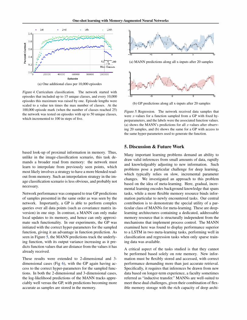
4.2.2. CURRICULUM TRAINING

Given the successful one-shot classification in episodeswith fifteen classes, we employed a curriculum trainingregime to further scale the classification capabilities of themodel. The network was first tasked to classify fifteenclasses per episode, and every 10,000 episodes of train-ing thereafter, the maximum number of classes presentedper episode incremented by one (Figure 4). The networkmaintained a high level of accuracy even as the numberof classes incremented higher throughout training. Aftertraining, at the 100,000 episode mark, the network wastested on episodes with 50 classes. Similar tests contin-ued, increasing the maximum number of classes to 100.The network generally exhibited gradually decaying per-formance as the number of classes increased towards 100.

(a) Five classes per episode

(b) Ten classes per episode

Figure 3. Persistent memory. To test the effects of interference,we did not wipe the external memory store from episode-to-episode. The network indeed struggled in this task (a), butnonetheless was able to perform comparably under certain setups,such as when episodes included ten classes and were of length 75(b).

The training limit of the network seemed to have not beenreached, as its performance continued to rise throughout upuntil the 100,000 episode mark. Assessing the maximumcapacity of the network offers an interesting opportunityfor future work.

4.3. Regression

Since our MANN architecture generated a broad strategyfor meta-learning, we reasoned that it would be able toadequately perform regression tasks on never-before-seenfunctions. To test this, we generated functions using froma GP prior with a fixed set of hyper-parameters and trainedour network using unique functions in each episode. Eachepisode involved the presentation of x-values (either 1, 2,or 3-dimensional) along with time-offset function values(i.e., f(xt−1)). A successful strategy involves the bindingof x-values with the appropriate function values and stor-age of these bindings in the external memory. Since indi-vidual x-values were only presented once per episode, suc-cessful function prediction involved an accurate content-


(a) One additional class per 10,000 episodes

Figure 4. Curriculum classification. The network started withepisodes that included up to 15 unique classes, and every 10,000episodes this maximum was raised by one. Episode lengths werescaled to a value ten times the max number of classes. At the100,000 episode mark (when the number of classes reached 25)the network was tested on episodes with up to 50 unique classes,which incremented to 100 in steps of five.

based look-up of proximal information in memory. Thus,unlike in the image-classification scenario, this task de-mands a broader read from memory: the network mustlearn to interpolate from previously seen points, whichmost likely involves a strategy to have a more blended read-out from memory. Such an interpolation strategy in the im-age classification scenario is less obvious, and probably notnecessary.

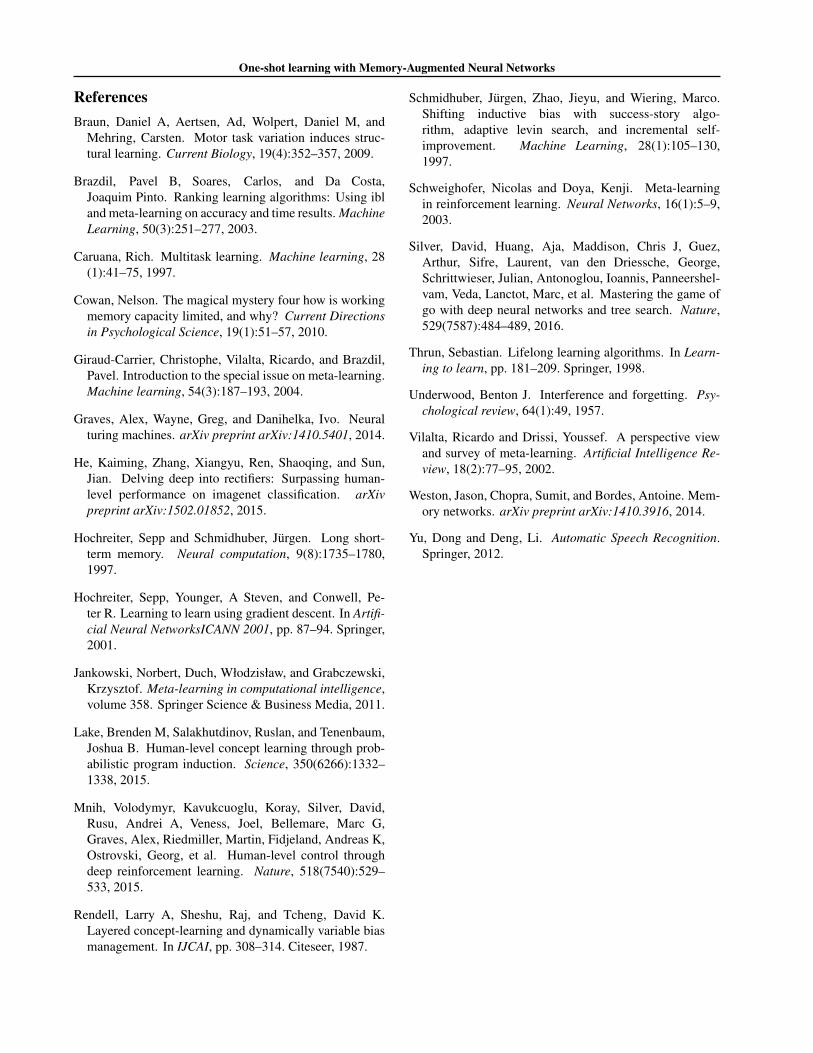
Network performance was compared to true GP predictionsof samples presented in the same order as was seen by thenetwork. Importantly, a GP is able to perform complexqueries over all data points (such as covariance matrix in-version) in one step. In contrast, a MANN can only makelocal updates to its memory, and hence can only approxi-mate such functionality. In our experiments, the GP wasinitiated with the correct hyper-parameters for the sampledfunction, giving it an advantage in function prediction. Asseen in Figure 5, the MANN predictions track the underly-ing function, with its output variance increasing as it pre-dicts function values that are distance from the values it hasalready received.

These results were extended to 2-dimensional and 3-dimensional cases (Fig 6), with the GP again having ac-cess to the correct hyper-parameters for the sampled func-tions. In both the 2-dimensional and 3-dimensional cases,the log-likelihood predictions of the MANN tracks appre-ciably well versus the GP, with predictions becoming moreaccurate as samples are stored in the memory.

(a) MANN predictions along all x-inputs after 20 samples

(b) GP predictions along all x-inputs after 20 samples

Figure 5. Regression. The network received data samples thatwere x-values for a function sampled from a GP with fixed hy-perparameters, and the labels were the associated function values.(a) shows the MANN’s predictions for all x-values after observ-ing 20 samples, and (b) shows the same for a GP with access tothe same hyper-parameters used to generate the function.

5. Discussion & Future WorkMany important learning problems demand an ability todraw valid inferences from small amounts of data, rapidlyand knowledgeably adjusting to new information. Suchproblems pose a particular challenge for deep learning,which typically relies on slow, incremental parameterchanges. We investigated an approach to this problembased on the idea of meta-learning. Here, gradual, incre-mental learning encodes background knowledge that spanstasks, while a more flexible memory resource binds infor-mation particular to newly encountered tasks. Our centralcontribution is to demonstrate the special utility of a par-ticular class of MANNs for meta-learning. These are deep-learning architectures containing a dedicated, addressablememory resource that is structurally independent from themechanisms that implement process control. The MANNexamined here was found to display performance superiorto a LSTM in two meta-learning tasks, performing well inclassification and regression tasks when only sparse train-ing data was available.

A critical aspect of the tasks studied is that they cannotbe performed based solely on rote memory. New infor-mation must be flexibly stored and accessed, with correctperformance demanding more than just accurate retrieval.Specifically, it requires that inferences be drawn from newdata based on longer-term experience, a faculty sometimesreferred as “inductive transfer.” MANNs are well-suited tomeet these dual challenges, given their combination of flex-ible memory storage with the rich capacity of deep archi-


Table 2. Test-set classification accuracies for various architectures on the Omniglot dataset after 100000 episodes of training, using five-character-long strings as labels. See the supplemental information for an explanation of 1st instance accuracies for the kNN classifier.

INSTANCE (% CORRECT)MODEL CONTROLLER # OF CLASSES 1ST 2ND 3RD 4TH 5TH 10TH

KNN (RAW PIXELS) – 5 4.0 36.7 41.9 45.7 48.1 57.0KNN (DEEP FEATURES) – 5 4.0 51.9 61.0 66.3 69.3 77.5FEEDFORWARD – 5 0.0 0.2 0.0 0.2 0.0 0.0LSTM – 5 0.0 9.0 14.2 16.9 21.8 25.5MANN FEEDFORWARD 5 0.0 8.0 16.2 25.2 30.9 46.8MANN LSTM 5 0.0 69.5 80.4 87.9 88.4 93.1

KNN (RAW PIXELS) – 15 0.5 18.7 23.3 26.5 29.1 37.0KNN (DEEP FEATURES) – 15 0.4 32.7 41.2 47.1 50.6 60.0FEEDFORWARD – 15 0.0 0.1 0.0 0.0 0.0 0.0LSTM – 15 0.0 2.2 2.9 4.3 5.6 12.7MANN (LRUA) FEEDFORWARD 15 0.1 12.8 22.3 28.8 32.2 43.4MANN (LRUA) LSTM 15 0.1 62.6 79.3 86.6 88.7 95.3MANN (NTM) LSTM 15 0.0 35.4 61.2 71.7 77.7 88.4

tectures for representation learning.

Meta-learning is recognized as a core ingredient of hu-man intelligence, and an essential test domain for evaluat-ing models of human cognition. Given recent successes inmodeling human skills with deep networks, it seems worth-while to ask whether MANNs embody a promising hypoth-esis concerning the mechanisms underlying human meta-learning. In informal comparisons against human subjects,the MANN employed in this paper displayed superior per-formance, even at set-sizes that would not be expected toovertax human working memory capacity. However, whenmemory is not cleared between tasks, the MANN suffersfrom proactive interference, as seen in many studies of hu-man memory and inference (Underwood, 1957). Thesepreliminary observations suggest that MANNs may pro-vide a useful heuristic model for further investigation intothe computational basis of human meta-learning.

The work we presented leaves several clear openings fornext-stage development. First, our experiments employeda new procedure for writing to memory that was prima fa-cie well suited to the tasks studied. It would be interestingto consider whether meta-learning can itself discover opti-mal memory-addressing procedures. Second, although wetested MANNs in settings where task parameters changedacross episodes, the tasks studied contained a high degreeof shared high-level structure. Training on a wider rangeof tasks would seem likely to reintroduce standard chal-lenges associated with continual learning, including therisk of catastrophic interference. Finally, it may be of inter-est to examine MANN performance in meta-learning tasksrequiring active learning, where observations must be ac-tively selected.

(a) 2D regression log-likelihoods within an episode

(b) 3D regression log-likelihoods within an episode

Figure 6. Multi-Dimensional Regression. (a) shows the negativelog likelihoods for 2D samples within a single episode, averagedacross 100 episodes, while (b) shows the same for 3D samples.


6. AcknowledgementsThe authors would like to thank Ivo Danihelka and GregWayne for helpful discussions and prior work on the NTMand LRU Access architectures, as well as Yori Zwols,and many others at Google DeepMind for reviewing themanuscript.


ReferencesBraun, Daniel A, Aertsen, Ad, Wolpert, Daniel M, and

Mehring, Carsten. Motor task variation induces struc-tural learning. Current Biology, 19(4):352–357, 2009.

Brazdil, Pavel B, Soares, Carlos, and Da Costa,Joaquim Pinto. Ranking learning algorithms: Using ibland meta-learning on accuracy and time results. MachineLearning, 50(3):251–277, 2003.

Caruana, Rich. Multitask learning. Machine learning, 28(1):41–75, 1997.

Cowan, Nelson. The magical mystery four how is workingmemory capacity limited, and why? Current Directionsin Psychological Science, 19(1):51–57, 2010.

Giraud-Carrier, Christophe, Vilalta, Ricardo, and Brazdil,Pavel. Introduction to the special issue on meta-learning.Machine learning, 54(3):187–193, 2004.

Graves, Alex, Wayne, Greg, and Danihelka, Ivo. Neuralturing machines. arXiv preprint arXiv:1410.5401, 2014.

He, Kaiming, Zhang, Xiangyu, Ren, Shaoqing, and Sun,Jian. Delving deep into rectifiers: Surpassing human-level performance on imagenet classification. arXivpreprint arXiv:1502.01852, 2015.

Hochreiter, Sepp and Schmidhuber, Jurgen. Long short-term memory. Neural computation, 9(8):1735–1780,1997.

Hochreiter, Sepp, Younger, A Steven, and Conwell, Pe-ter R. Learning to learn using gradient descent. In Artifi-cial Neural NetworksICANN 2001, pp. 87–94. Springer,2001.

Jankowski, Norbert, Duch, Włodzisław, and Grabczewski,Krzysztof. Meta-learning in computational intelligence,volume 358. Springer Science & Business Media, 2011.

Lake, Brenden M, Salakhutdinov, Ruslan, and Tenenbaum,Joshua B. Human-level concept learning through prob-abilistic program induction. Science, 350(6266):1332–1338, 2015.

Mnih, Volodymyr, Kavukcuoglu, Koray, Silver, David,Rusu, Andrei A, Veness, Joel, Bellemare, Marc G,Graves, Alex, Riedmiller, Martin, Fidjeland, Andreas K,Ostrovski, Georg, et al. Human-level control throughdeep reinforcement learning. Nature, 518(7540):529–533, 2015.

Rendell, Larry A, Sheshu, Raj, and Tcheng, David K.Layered concept-learning and dynamically variable biasmanagement. In IJCAI, pp. 308–314. Citeseer, 1987.

Schmidhuber, Jurgen, Zhao, Jieyu, and Wiering, Marco.Shifting inductive bias with success-story algo-rithm, adaptive levin search, and incremental self-improvement. Machine Learning, 28(1):105–130,1997.

Schweighofer, Nicolas and Doya, Kenji. Meta-learningin reinforcement learning. Neural Networks, 16(1):5–9,2003.

Silver, David, Huang, Aja, Maddison, Chris J, Guez,Arthur, Sifre, Laurent, van den Driessche, George,Schrittwieser, Julian, Antonoglou, Ioannis, Panneershel-vam, Veda, Lanctot, Marc, et al. Mastering the game ofgo with deep neural networks and tree search. Nature,529(7587):484–489, 2016.

Thrun, Sebastian. Lifelong learning algorithms. In Learn-ing to learn, pp. 181–209. Springer, 1998.

Underwood, Benton J. Interference and forgetting. Psy-chological review, 64(1):49, 1957.

Vilalta, Ricardo and Drissi, Youssef. A perspective viewand survey of meta-learning. Artificial Intelligence Re-view, 18(2):77–95, 2002.

Weston, Jason, Chopra, Sumit, and Bordes, Antoine. Mem-ory networks. arXiv preprint arXiv:1410.3916, 2014.

Yu, Dong and Deng, Li. Automatic Speech Recognition.Springer, 2012.


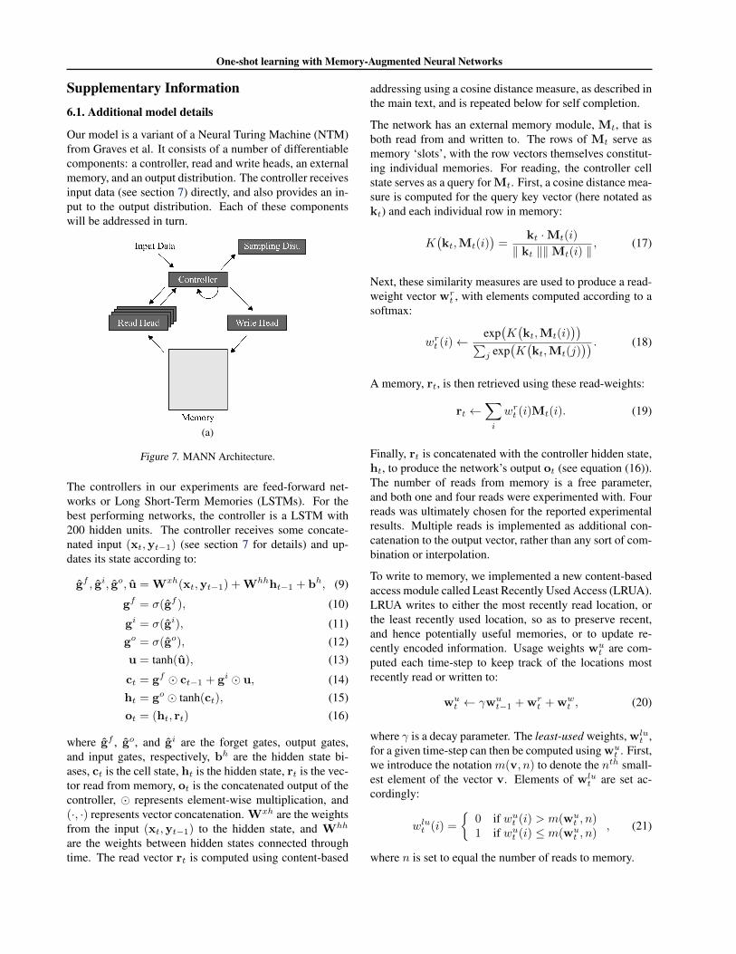
Supplementary Information6.1. Additional model details

Our model is a variant of a Neural Turing Machine (NTM)from Graves et al. It consists of a number of differentiablecomponents: a controller, read and write heads, an externalmemory, and an output distribution. The controller receivesinput data (see section 7) directly, and also provides an in-put to the output distribution. Each of these componentswill be addressed in turn.

(a)

Figure 7. MANN Architecture.

The controllers in our experiments are feed-forward net-works or Long Short-Term Memories (LSTMs). For thebest performing networks, the controller is a LSTM with200 hidden units. The controller receives some concate-nated input (xt,yt−1) (see section 7 for details) and up-dates its state according to:

gf , gi, go, u = Wxh(xt,yt−1) +Whhht−1 + bh, (9)

gf = σ(gf ), (10)

gi = σ(gi), (11)go = σ(go), (12)u = tanh(u), (13)

ct = gf � ct−1 + gi � u, (14)ht = go � tanh(ct), (15)ot = (ht, rt) (16)

where gf , go, and gi are the forget gates, output gates,and input gates, respectively, bh are the hidden state bi-ases, ct is the cell state, ht is the hidden state, rt is the vec-tor read from memory, ot is the concatenated output of thecontroller, � represents element-wise multiplication, and(·, ·) represents vector concatenation. Wxh are the weightsfrom the input (xt,yt−1) to the hidden state, and Whh

are the weights between hidden states connected throughtime. The read vector rt is computed using content-based

addressing using a cosine distance measure, as described inthe main text, and is repeated below for self completion.

The network has an external memory module, Mt, that isboth read from and written to. The rows of Mt serve asmemory ‘slots’, with the row vectors themselves constitut-ing individual memories. For reading, the controller cellstate serves as a query for Mt. First, a cosine distance mea-sure is computed for the query key vector (here notated askt) and each individual row in memory:

K(kt,Mt(i)

)=

kt ·Mt(i)

‖ kt ‖‖Mt(i) ‖, (17)

Next, these similarity measures are used to produce a read-weight vector wr

t , with elements computed according to asoftmax:

wrt (i)←exp(K(kt,Mt(i)

))∑j exp

(K(kt,Mt(j)

)) . (18)

A memory, rt, is then retrieved using these read-weights:

rt ←∑i

wrt (i)Mt(i). (19)

Finally, rt is concatenated with the controller hidden state,ht, to produce the network’s output ot (see equation (16)).The number of reads from memory is a free parameter,and both one and four reads were experimented with. Fourreads was ultimately chosen for the reported experimentalresults. Multiple reads is implemented as additional con-catenation to the output vector, rather than any sort of com-bination or interpolation.

To write to memory, we implemented a new content-basedaccess module called Least Recently Used Access (LRUA).LRUA writes to either the most recently read location, orthe least recently used location, so as to preserve recent,and hence potentially useful memories, or to update re-cently encoded information. Usage weights wu

t are com-puted each time-step to keep track of the locations mostrecently read or written to:

wut ← γwu

t−1 +wrt +ww

t , (20)

where γ is a decay parameter. The least-used weights, wlut ,

for a given time-step can then be computed using wut . First,

we introduce the notation m(v, n) to denote the nth small-est element of the vector v. Elements of wlu

t are set ac-cordingly:

wlut (i) =

{0 if wut (i) > m(wu

t , n)1 if wut (i) ≤ m(wu

t , n), (21)

where n is set to equal the number of reads to memory.


To obtain the write weights wwt , a learnable sigmoid gate

parameter is used to compute a convex combination of theprevious read weights and previous least-used weights:

wwt ← σ(α)wr

t−1 + (1− σ(α))wlut−1, (22)

where α is a dynamic scalar gate parameter to interpolatebetween the weights. Prior to writing to memory, the leastused memory location is computed from wu

t−1 and is set tozero. Writing to memory then occurs in accordance withthe computed vector of write weights:

Mt(i)←Mt−1(i) + wwt (i)kt,∀i (23)

6.2. Output distribution

The controller’s output, ot, is propagated to an output dis-tribution. For classification tasks using one-hot labels, thecontroller output is first passed through a linear layer withan output size equal to the number of classes to be classi-fied per episode. This linear layer output is then passed asinput to the output distribution. For one-hot classification,the output distribution is a categorical distribution, imple-mented as a softmax function. The categorical distributionproduces a vector of class probabilities, pt, with elements:

pt(i) =exp(Wop(i)ot)∑j exp(Won(j)ot)

, (24)

where Wop are the weights from the controller output tothe linear layer output.

For classification using string labels, the linear output sizeis kept at 25. This allows for the output to be split intofive equal parts each of size five. Each of these parts isthen sent to an independent categorical distribution thatcomputes probabilities across its five inputs. Thus, eachof these categorical distributions independently predicts a‘letter,’ and these letters are then concatenated to producethe five-character-long string label that serves as the net-work’s class prediction (see figure 8).

A similar implementation is used for regression tasks. Thelinear output from the controller outputs two values: µ andσ, which are passed to a Gaussian distribution sampler aspredicted mean and variance values. The Gaussian sam-pling distribution then computes probabilities for the targetvalue yt using these values.

6.3. Learning

For one-hot label classification, given the probabilities out-put by the network, pt, the network minimizes the episodeloss of the input sequence:

L(θ) = −∑t

yTt logpt, (25)

where yt is the target one-hot or string label at time t (note:for a given one-hot class-label vector yt, only one elementassumes the value 1, and for a string-label vector, five ele-ments assume the value 1, one per five-element ‘chunk’).

For string label classification, the loss is similar:

L(θ) = −∑t

∑c

yTt (c) logpt(c). (26)

Here, the (c) indexes a five-element long ‘chunk’ of thevector label, of which there are a total of five.

For regression, the network’s output distribution is a Gaus-sian, and as such receives two-values from the controlleroutput’s linear layer at each time-step: predictive µ and σvalues, which parameterize the output distribution. Thus,the network minimizes the negative log-probabilities as de-termined by the Gaussian output distribution given theseparameters and the true target yt.

7. Classification input dataInput sequences consist of flattened, pixel-level representa-tions of images xt and time-offset labels yt−1 (see figure8 for an example sequence of images and class identitiesfor an episode of length 50, with five unique classes). First,N unique classes are sampled from the Omniglot dataset,where N is the maximum number of unique classes perepisode. N assumes a value of either 5, 10, or 15, whichis indicated in the experiment description or table of resultsin the main text. Samples from the Omniglot source setare pulled, and are kept if they are members of the set of nunique classes for that given episode, and discarded other-wise. 10N samples are kept, and constitute the image datafor the episode. And so, in this setup, the number of sam-ples per unique class are not necessarily equal, and someclasses may not have any representative samples. Omniglotimages are augmented by applying a random rotation uni-formly sampled between − π

16 and π16 , and by applying a

random translation in the x- and y- dimensions uniformlysampled between -10 and 10 pixels. The images are thendownscaled to 20x20. A larger class-dependent rotation isthen applied, wherein each sample from a particular class isrotated by either 0, π2 , π, or 3π

2 (note: this class-specific ro-tation is randomized each episode, so a given class may ex-perience different rotations from episode-to-episode). Theimage is then flattened into a vector, concatenated with arandomly chosen, episode-specific label, and fed as inputto the network controller.

Class labels are randomly chosen for each class fromepisode-to-episode. For one-hot label experiments, labelsare of size N , where N is the maximum number of uniqueclasses that can appear in a given episode.


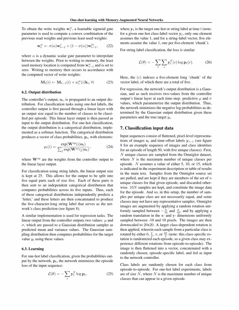
(a) String label encoded as five-hot vector

(b) Input Sequence

Figure 8. Example string label and input sequence.

8. TaskEither 5, 10, or 15 unique classes are chosen per episode.Episode lengths are ten times the number of unique classes(i.e., 50, 100, or 150 respectively), unless explicitly men-tioned otherwise. Training occurs for 100 000 episodes.At the 100 000 episode mark, the task continues; however,data are pulled from a disjoint test set (i.e., samples fromclasses 1201-1623 in the omniglot dataset), and weight up-dates are ceased. This is deemed the “test phase.”

For curriculum training, the maximum number of uniqueclasses per episode increments by 1 every 10 000 trainingepisodes. Accordingly, the episode length increases to 10times this new maximum.

9. Parameters9.0.1. OPTIMIZATION

Rmsprop was used with a learning rate of 1e−4 and maxlearning rate of 5e−1, decay of 0.95 and momentum 0.9.

9.0.2. FREE PARAMETER GRID SEARCH

A grid search was performed over number of parameters,with the values used shown in parentheses: memory slots(128), memory size (40), controller size (200 hidden units

for a LSTM), learning rate (1e−4), and number of readsfrom memory (4). Other free parameters were left con-stant: usage decay of the write weights (0.99), minibatchsize (16),

9.1. Comparisons and controls evaluation metrics

9.1.1. HUMAN COMPARISON

For the human comparison task, participants perform theexact same experiment as the network: they observe se-quences of images and time-offset labels (sequence length= 50, number of unique classes = 5), and are challengedto predict the class identity for the current input image byinputting a single digit on a keypad. However, partici-pants view class labels the integers 1 through 5, rather thanone-hot vectors or strings. There is no time limit for theirchoice. Participants are made aware of the goals of the taskprior to starting, and they perform a single, non-scored trialrun prior to their scored trials. Nine participants each per-formed two scored trials.

9.1.2. KNN

When no data is available (i.e., at the start of training), thekNN classifier randomly returns a single class as its pre-diction. So, for the first data point, the probability that theprediction is correct is 1

N where N is number of uniqueclasses in a given episode. Thereafter, it predicts a classfrom classes that it has observed. So, all instances of sam-ples that are not members of the first observed class cannotbe correctly classified until at least one instance is passedto the classifier. Since statistics are averaged across classes,first instance accuracy becomes 1

N ( 1N +0) = 1

N2 , which is4% and 0.4% for 5 and 15 classes per episode, respectively.

one-shot learning with memory-augmented neural networks · one-shot learning with memory-augmented...

Documents