online cash management for businesses

econstorMake Your Publications Visible.

A Service of

zbwLeibniz-InformationszentrumWirtschaftLeibniz Information Centrefor Economics

Mahagaonkar, Prashanth; Qiu, Jianying

Working Paper

Testing the Modigliani-Miller theorem directly in thelab: a general equilibrium approach

Jena economic research papers, No. 2008,056

Provided in Cooperation with:Max Planck Institute of Economics

Suggested Citation: Mahagaonkar, Prashanth; Qiu, Jianying (2008) : Testing the Modigliani-Miller theorem directly in the lab: a general equilibrium approach, Jena economic researchpapers, No. 2008,056, Universität Jena und Max-Planck-Institut für Ökonomik, Jena

This Version is available at:http://hdl.handle.net/10419/25738

Standard-Nutzungsbedingungen:

Die Dokumente auf EconStor dürfen zu eigenen wissenschaftlichenZwecken und zum Privatgebrauch gespeichert und kopiert werden.

Sie dürfen die Dokumente nicht für öffentliche oder kommerzielleZwecke vervielfältigen, öffentlich ausstellen, öffentlich zugänglichmachen, vertreiben oder anderweitig nutzen.

Sofern die Verfasser die Dokumente unter Open-Content-Lizenzen(insbesondere CC-Lizenzen) zur Verfügung gestellt haben sollten,gelten abweichend von diesen Nutzungsbedingungen die in der dortgenannten Lizenz gewährten Nutzungsrechte.

Terms of use:

Documents in EconStor may be saved and copied for yourpersonal and scholarly purposes.

You are not to copy documents for public or commercialpurposes, to exhibit the documents publicly, to make thempublicly available on the internet, or to distribute or otherwiseuse the documents in public.

If the documents have been made available under an OpenContent Licence (especially Creative Commons Licences), youmay exercise further usage rights as specified in the indicatedlicence.

www.econstor.eu

JENA ECONOMIC RESEARCH PAPERS

# 2008 – 056

Testing the Modigliani-Miller theorem directly in the lab: a general equilibrium approach

by

Prashanth Mahagaonkar Jianying Qiu

www.jenecon.de

ISSN 1864-7057

The JENA ECONOMIC RESEARCH PAPERS is a joint publication of the Friedrich Schiller University and the Max Planck Institute of Economics, Jena, Germany. For editorial correspondence please contact [email protected]. Impressum: Friedrich Schiller University Jena Max Planck Institute of Economics Carl-Zeiss-Str. 3 Kahlaische Str. 10 D-07743 Jena D-07745 Jena www.uni-jena.de www.econ.mpg.de © by the author.

http://www.uni-jena.de/

http://www.econ.mpg.de/

Testing the Modigliani-Miller theorem directly in the lab:

a general equilibrium approach

Prashanth Mahagaonkar∗ Jianying Qiu†‡

Abstract

In this paper, we experimentally test the Modigliani-Miller theorem. Applying ageneral equilibrium approach and not allowing for arbitrage among firms with differ-ent capital structure, we are able to address a question fundamental to the valuationof firms: does capital structure affect the value of the firm? If so, how? We find that,consistent with the Modigliani-Miller theorem, experimental subjects well recognizedthe increased systematic risk of the equity with increasing leverage and accordinglydemanded higher rate of return. Yet, this adjustment was not perfect: subjects un-derestimated the systematic risk of low leveraged equity whereas overestimated thesystematic risk of high leveraged equity, resulting in a U shape weighted average costof capital.

JEL Classification: G32, C91, G12, D53,

Keywords: The Modigliani-Miller Theorem, Experimental Study, Decision Making underUncertainty, General Equilibrium

∗Max Planck Institute of Economics, EGP Group, Kahlaische Str. 10, D-07745 Jena, Germany.

†Max Planck Institute of Economics, ESI Group, Kahlaische Str. 10, D-07745 Jena, Germany.

‡Corresponding author : Max Planck Institute of Economics, ESI Group, Kahlaische Str. 10, D-07745Jena, Germany. Tel.: +49-(0)3641-686633; fax: +49-(0)3641-686667. E-mail address: [email protected].

§We would like to thank Werner Guth, Rene Levinsky, Birendra Kumar Rai, Ondrej Rydval, ChristophVanberg, and Anthony Ziegelmeyer for their helpful comments and suggestions.

Jena Economic Research Papers 2008 - 056

1 Introduction

Ever since the appearance of Modigliani and Miller (1958) (commonly known as ‘MM’theorem), there has been substantial effort in testing the Modigliani-Miller theorem. Therehas been enormous evidence supporting as well as refuting the propositions. The 1958paper Modigliani and Miller (1958) itself had a section devoted to testing the propositionson oil and electricity utility industry and found little association between leverage andcost of capital. Later in Miller and Modiglian (1966), they performed a test using a two-stage instrumental variable approach on electric utility industry in the United States andfound no evidence for “sizeable leverage or dividend effects of the kind assumed in muchof the traditional literature of finance”. Davenport (1971) uses British data on threeindustry groups, chemicals, food and metal manufacturing, and finds that the overall costof capital is independent of the capital structure. The opposition to the MM theoremscame from many angles. Weston (1963) in a cross sectional study on electric utilities andoil companies finds that firm’s value increases with leverage. Robichek et al. (1967) findresults consistent with a gain from leverage. Masulis (1980), Pinegar and Lease (1986),and Lee (1987) also find similar results. After thirty years of debate and testing, Miller(1988) conceded: “Our hopes of settling the empirical issues . . .,however, have largely beendisappointed.”This is the fiftieth year of the paper and still the opinion may hold true.

After the 80s the direct testing of the Modigliani-Miller theorem using field data seemsto have been given less focus, or simply forgotten. This is quite understandable given theunfruitful debate so far, and that a clean testing of the theorem using real market data isbasically impossible due to the restrictions and assumptions that the theorem demands.Firstly, capital structure is difficult to measure. An accurate market estimate of publiclyheld debt is already difficult and to get a good market value data on privately held debt isalmost impossible. The complex liability structure that firms face complicates this matterfurther, e.g., pension liabilities, deferred compensation to management and employees, andcontingent securities such as warrants, convertible debt, and convertible preferred stock.Secondly, it is nearly impossible to effectively disentangle the impact of capital structureon the value of firms from the effects of other fundamental changes. Myers (2001) thereforerightly admits, “the Modigliani and Miller (1958) paper is exceptionally difficult to testdirectly”.

In this paper, we reopen the issue and test the Modigliani-Miller theorem directly via alaboratory experiment. Compared to field works, laboratory studies offer more control.Changes of firms’ other aspects can be minimized while the capital structure of firms areadjusted, and the capital structure of the firm can be easily measured. By constructing a

1


testing environment as close as possible to the theoretical model, we want to see whether,nonetheless, experimental subjects value firms differently. We adapted our experimentmodel from the theoretical model of (Stiglitz, 1969). Using a general equilibrium ap-proach, we are able to show that, when individuals can borrow at the same market rate ofinterest as firms and there is no bankruptcy, the Modigliani-Miller theorem always holdsin equilibrium, and that this result does not depend on individuals’ risk attitudes andinitial wealth positions.

The remainder of the paper is organized as follows. In section 2, we first discuss the U

shape weighted average cost of capital approach and demonstrate its defective link. Thenwe introduce the Modigliani-Miller theorem and a theoretical model for the experimentbasing on Stiglitz (1969). In section 3 the experimental design is presented. Results arereported in section 4 and section 5 concludes.

2 Theories of the cost of capital

Before 1958, the cost of capital was thought to possess a U shape. The argument runs asfollows: equity is risky and thus more costly, while debt is not or at least much less risky1.Therefore a firm can reduce its cost of capital by issuing some debt in exchange for someof its equity. As the debt equity ratio increases further, default risk becomes large andafter some point debt becomes more expensive than equity.

To make it clearer, let us consider a firm with a market value of debts B, and a marketvalue of shares S. Let τ = B

V denote the leverage ratio, i denote the expected rate ofreturn on equity, and r the rate of return on debts. Then the unit cost of capital , ρ, issimply the weighted average of i and r:

ρ =X

V=

S

Vi +

B

Vr (1)

= (1− τ) · i + τ · r.

In the U shape of the cost of capital approach, it is assumed that i is independent of τ ,whereas r is a function of τ . More specifically, r < i when τ is small and r > i when τ

1A firm promises to make contractual payments no matter what the earnings are. Thus there can existno risk when there is no bankruptcy possibility. When there is bankruptcy possibility, since debt haspriority over equity in payment, it is still the less risky one

2


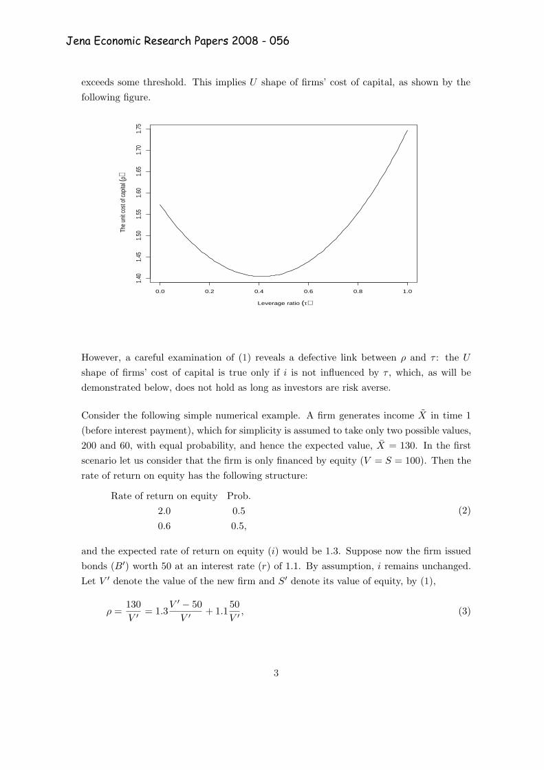
exceeds some threshold. This implies U shape of firms’ cost of capital, as shown by thefollowing figure.

0.0 0.2 0.4 0.6 0.8 1.0

1.40

1.45

1.50

1.55

1.60

1.65

1.70

1.75

Leverage ratio (τ)

The

unit

cost

of c

apita

l (ρ)

However, a careful examination of (1) reveals a defective link between ρ and τ : the U

shape of firms’ cost of capital is true only if i is not influenced by τ , which, as will bedemonstrated below, does not hold as long as investors are risk averse.

Consider the following simple numerical example. A firm generates income X in time 1(before interest payment), which for simplicity is assumed to take only two possible values,200 and 60, with equal probability, and hence the expected value, X = 130. In the firstscenario let us consider that the firm is only financed by equity (V = S = 100). Then therate of return on equity has the following structure:

Rate of return on equity Prob.2.0 0.50.6 0.5,

(2)

and the expected rate of return on equity (i) would be 1.3. Suppose now the firm issuedbonds (B′) worth 50 at an interest rate (r) of 1.1. By assumption, i remains unchanged.Let V ′ denote the value of the new firm and S′ denote its value of equity, by (1),

ρ =130V ′ = 1.3

V ′ − 50V ′ + 1.1

50V ′ , (3)

3


which implies V ′ ≈ 108, and thus S′ ≈ 58. The rate of return on equity is then:

Rate of return on equity Prob.200−50×1.1

58 0.560−50×1.1

58 0.5

≈Rate of return on equity Prob.

2.5 0.50.1 0.5.

(4)

Notice that, investors ask for the same rate of return for a income flow with higher risk.As suggested by standard financial theory, this can not happen as long as investors arerisk averse.

In fact, above example has already revealed the intuition of the Modigliani-Miller theorem(hereafter the MM theorem). Recognizing the relationship between τ and i, Proposition Iof Modigliani and Miller (1958) argues that:The market value of any firm is independent of its capital structure and is given by capi-talizing its expected return at some rate ρ appropriate to its risk level.

2.1 The Methodology

In examining the Modigliani-Miller theorem, there are several approaches that might betaken. A natural approach is to take the Modigliani and Miller (1958) model where ar-bitrage among firms are possible. But, in this paper, we shall take a rather differentapproach. We ask experimental subjects to evaluate the equity of firms with differentcapital structure separately in different markets, one firm in each market. No arbitrageamong these firms is possible.

Arbitrage process plays an important role in Modigliani and Miller (1958); it helps torestore the Modigliani-Miller theorem once it is violated. But, as shown by Hirshleifer(1966) and Stiglitz (1969), arbitrage is not necessary for The Modigliani-Miller theo-rem to hold. Moreover, allowing for arbitrage among firms may exclude one potentiallyinteresting phenomena: suppose there are systematic preferences for firms with partic-ular capital structure, this ‘anomaly’ would not be observed on the market level sinceit would be eliminated away by a few arbitragers, and it would have been interesting ifwe can observe this anomaly and understand why it occurs. After all, as demonstratedby Shleifer and Vishny (1997), arbitrage can never be complete in real financial markets.Thus, by excluding arbitrage among firms it allows us to address a question fundamentalto the valuation of firms: Do subjects systematically evaluate firms with different capitalstructure differently? If so, how?

4


There is an additional strength in proceeding this way. Some empirical studies showthat firms with different capital structures are valuated similarly. However, this does notnecessarily imply the irrelevance of capital structure to the valuation of the firm. It couldbe that, although investors in general preferred some capital structures τ∗ to some othercapital structures τ ′, these preferences would not be revealed on the market level sincefirms - recognizing investors’ preferences - would adjust their capital structure towards τ∗.As a result, firms are valuated similarly, but concentrated on some capital structures τ∗.Our approach would allow us also to address this possibility.

Not allowing for arbitrage among firms, however, does cause one potential serious problem:the law of one price can not be applied any more. The law of one price states that the samegoods must sell at the same price in the same market. Our experimental design effectivelycuts the link among firms, and make the markets for different firms independent from eachother. It is then difficult to guarantee that the market conditions, including market rulesand traits of market participants, are the same for different firms. This could seriouslyblur the message of experimental results. For example, the same lottery ticket is usuallyvaluated differently by millionaires and poor people, but this difference reflects not thedifference of lottery tickets but the heterogeneity of market participants. More specifically,differences in the values of the firms in the economy not allowing for arbitrage among firmswith different capital structures could be due to two possibilities:

1. market participants apply a valuation process by which firms with different capitalstructures are valued differently, or

2. participants with certain traits have inherent preferences for equity with a particularincome pattern, e.g., due to portfolio diversification reason.

The second possibility is especially relevant in the current setting since experimental sub-jects are mainly students and they share similar financial backgrounds. Without propercontrol, this problem of sample selection could significantly limit the validity of our results.Even if systematic differences in the values of the firms are found, it might not be relevanton market level; it might be a special case pertaining only to our subjects.

Since the first possibility will be our main focus, a proper model should minimize the secondpossibility. For this purpose, we base adapt the model of Stiglitz (1969). Stiglitz (1969)puts forward a general equilibrium model, and it can be shown that the Modigliani-Millertheorem holds regardless the initial wealth condition of market participants. Furthermore,the equilibrium solution in Stiglitz (1969) is derived by the state preference approach.

5


Comparing to the more familiar mean-variability approach, i.e. mean-variance approach,this approach does not make strong assumptions about risk attitudes or the shape of theutility function. Hence the results hold under more general conditions.

2.2 The Model

For simplicity consider an economy where there is one firm which exists for two periods:now (denoted by t0) and future (denoted by t1). The market values of firm’s equity anddebt are respectively S and B, and hence the market value of the firm is

V = B + S.

The uncertain income stream X generated by firm i at date t1 is a function of the stateθ ∈ Θ, and X(θ) denotes firm’s income in state θ. There are n investors, and the set ofinvestors is denoted by N . Each investor i is endowed with an initial wealth of ωi, which iscomposed of a fraction αi of equity S, and Bi unit of bonds. Since the economy is closed,we have

∑

i∈N

αi = 1,∑

i∈N

Bi = B, (5)

By convention, one unit of bond costs one unit of money, thus

ωi = αiS + Bi. (6)

In addition, there exists a credit market, where both the firm and investors can borrow orlend at the rate of interest r. To be consistent with the assumptions of Modigliani-Millertheorem, we assume the firm never goes bankrupt. Investors prefer more to less. Moreover,all investors are assumed to evaluate alternative portfolios in terms of the income streamthey generate, i.e., investors’ preferences are not state dependent.

2.2.1 The Benchmark Solution

In this section, we shall first prove the following proposition:

Proposition 1 (1)If there exists a general equilibrium with the firm fully equity financedand having a particular value, then there exists another general equilibrium solution forthe economy with the firm having any other capital structure but with the value of the firm

6


remains unchanged. (2)Moreover, this holds in any equilibrium.2

Let us now consider two economies where the firm in the first economy is only financed byequity and the firm in the second economy is financed by bonds and equity. Let V1 andV2 denote the value of the firm in the first and second economy, respectively. We now tryto show that there exists a general equilibrium solution with V2 = V1.

Consider the first economy, since here the firm issues no bonds (B), we have V1 = S1, and∑i∈N B1

i = 0. Here a positive (negative) value of B1i would mean that investor i invests

(borrows) B1i units of money in (from) the credit market. Let Y 1

i (θ) denote investor i’sincome in state θ. With the portfolio of αi shares and B1

i units of bonds, investor i’sreturn in state θ may be written as:

Y 1i (θ) = αiX(θ) + rB1

i (7)

= αiX(θ) + r(ωi − αiV1)

which follows by S1 = V1 and (6).

Consider now the second economy where the firm issues bonds with a market value of B2.Let S2 denote the value of the firm’s equity in this economy, we have the value of the firmV2 = S2 + B2 and

∑i∈N B2

i = B2. Notice that the firm generates the same pattern ofincome stream X. With a portfolio of αi fraction of equity and Bi units of bonds, investori’s return in state θ is then given by:

Y 2i (θ) = αi(X(θ)− rB2) + rB2

i

= αi(X(θ)− rB2) + r(ωi − αiS2)

= αiX(θ) + r(ωi − αiV2), (8)

where the third equality follows by S2 = V2 −B2.

If V1 = V2 = V ∗, the opportunity sets of individual i in both economies, Y 1i (θ) and Y 2

i (θ),will be identical:

Y 1i (θ) = Y 2

i (θ) for∀θ ∈ Θ. (9)

2Stiglitz (1969) only proves the first part of proposition 1. We complete the following proposition bydemonstrating the second part of proposition 1.

7


If the vector ({α∗i }i∈I) maximizes individual’s utility in the first economy, it still does inthe second economy. This proves the first part of proposition 1. It remains to show thatV1 = V2 = V ∗ must hold in any equilibrium when agents are strictly risk averse.

Suppose there exists an equilibrium in the second economy where V ′2 > V1 = V ∗. This

in turn implies S′2 = V ′2 − B2 > V ∗ − B2 = S∗2 . Notice that equity’s rate of return is

calculated as X−rBS , with X and B remaining unchanged, the increase of equity value

from S∗2 to S′2 decreases equity’s rate of return. However, given any risk composition ofthe second economy, the decrease of equity’s rate of return discourages the demand forequity. Since the equity market of the second economy clears at S∗2 = V ∗ −B2, it followsthen there will be over supply of equity when S′2 > S∗2 . A contradiction to V ′

2 > V ∗ beingan equilibrium. The other case V ′

2 < V ∗ can be proven similarly.

Several features of the model are worth noticing. Firstly, no assumptions on investors’initial wealth position are made, which is particularly helpful when conducting laboratoryexperiments because it reduces effects of sample selection on results. Secondly, except forthe basic assumption that investors prefer more to less, no strong assumption about theshape of investors’ utility function are made. This is also very appealing since measuringsubjects’ risk attitudes are tricky and inaccurate. Therefore, we expect experimentalresults based upon the above model to hold in broad circumstances.

3 Experimental Protocol

The computerized experiment was conducted in September 2007. Overall, we ran 2 sessionswith a total of 64 subjects, all being students at the University of Jena. The two sessionswere run in the computer lab of the Max Planck Institute of Economics in Jena (Ger-many). The experiment was programmed using the Z-Tree software (Fischbacher, 1999).Considering the complexity of experimental procedure, only students with relatively highanalytical skills were invited, e.g., students majoring in mathematics, economics, businessadministration, or physics.

3.1 General Environments and Procedures

Each experimental session consists of two subsequent phases. In the first phase, subjects’risk attitudes are measured using table 4 (Holt and Laury, 2002). In table 4, each rowdenotes one choice situation. In each choice situation, option Y pays out 50 ECU (Experi-

8


mental Currency Unit) with certainty, and option X yields 2 possible monetary outcomes,70 ECU and 30 ECU that are paid out according to the probabilities noted. While thetwo possible outcomes remain constant in all 10 choice situations, their probabilities vary.Subjects are asked to choose between X and Y for each of ten choice situations. After theymake their decisions, one of the 10 choice situations is randomly chosen. Subjects’ exper-imental earnings depend on their choices in the chosen situation. However, in order notto affect subjects’ risk attitudes in the following phase, experimental earnings for the firstphase are not announced yet. They are announced at the end of the whole experiment,together with their earnings in the second phase of the experiment.

In the second phase, subjects are divided into 4 independent groups, with 8 subjectseach. Group compositions are kept constant through out this phase. The second phase ofexperiment consists of 8 treatments (in the experiment, treatments are referred as rounds)i.e., we compare treatments within subjects.

The experimental environments in each treatment are constructed as close as possible tothe theoretical model. Firms are represented by a risky asset generating income flow:

X =

{1200 if θ = good800 if θ = bad.

For simplicity, we impose

Prob(θ = good) = Prob(θ = bad) =12.

Firms have 100 shares outstanding and differ only in the market value of debts B. Sincethere is no bankruptcy possibility, bonds are perfectly safe, and one unit of money investedin bonds yielded a gross return of 1.5, that is, the net risk-free interest rate is 0.5. Subjectsare told they can borrow any amount of money from a bank at this interest rate.

In each treatment, only one firm is evaluated through a market mechanism (to be ex-plained shortly), hence valuation of firms are independent from treatment to treatment:subjects’ decisions in one treatment do not not affect their play in other treatments. Tofurther discourage (potential) portfolio effects, only one treatment is randomly selectedfor experimental payment. The sequence that firms are evaluated across 8 treatments arecharacterized by the market value of bonds B:

Treatments 1 2 3 4 5 6 7 8Bond value 50 ⇒ 350 ⇒ 100 ⇒ 0 ⇒ 400 ⇒ 200 ⇒ 500 ⇒ 300,

9


where the first two treatments are for training, and the last 6 are formal treatments.However, in the experiment, subjects are not presented with above structures. Instead,they are asked to evaluate the resulting equities of firms after the interest payment of debthas been deducted:

1

Gain Prob.

11.25 0.57.25 0.5

=⇒ 2

Gain Prob.

6.75 0.52.75 0.5

=⇒ 3

Gain Prob.

10.50 0.56.50 0.5

=⇒

4

Gain Prob.

12.00 0.58.00 0.5

=⇒ 5

Gain Prob.

6.00 0.52.00 0.5

=⇒ 6

Gain Prob.

9.00 0.55.00 0.5

=⇒

7

Gain Prob.

4.50 0.50.50 0.5

=⇒ 8

Gain Prob.

7.50 0.53.50 0.5.

(10)

Here the concern is that some of the subjects may have learned the Modigliani-Millertheorem in the past, and with complete capital structure (firms’ income flow and themarket value of bond), they may try to be consistent with the Modigliani-Miller theoremand thereby bias the results. Presenting them only with the resulting equities shouldsignificantly increase their difficulty in doing so.

More specifically, the experimental procedure in each treatment follows thus:

1. At the beginning of each treatment, subjects are presented with a risky alternative:one of the resulting equity of a firm shown in (10). In addition, they receive someinitial endowments.

2. A market mechanism becomes available, with which subjects in each group can tradethe risky alternative with each other. Trading quantity can only be of integers andshort selling is not allowed. Notice that the highest possible value of a unit of equityis (1200−B)/100, and the lowest possible value of a unit of equity is (800−B)/(100×1.5),buying or selling prices are restricted to the range of [(1200−B)/100, (800−B)/(100×1.5)].

3. After some time, the market closes. When subjects have a net change in share holdingafter the market process, the agent should either (a) pay a per-unit price equal to themarket-clearing price for each unit of equity he purchased, which is be automaticallydeducted from the money in their bank account, or (b) receive a per-unit price equalto the market-clearing price for each unit he sold, which is automatically depositedinto the bank and earn a risk-free interest rate of 0.5. Subjects then receive thefollowing information:

• the market clearing price;

• own final holding of equity αi and bonds Bi.

10


Notice that the information about the realized state are not given here. This is to decreaseincome or wealth effects. Instead, this information is given at the end of the this phase3.

The feedback information subjects receive at the end of this phase is: (1) the state ofworld realized for each treatment; (2) own net profit in each treatment; (3) the randomlychosen treatment for payment; (4) own final experimental earning.

To provide subjects with stronger marginal incentive and increase the cost of makingmistakes so that subjects take decisions more seriously, we grant subjects an initial en-dowment as risk free credit and pay them only the net profits they make. We now describethe structure of this initial endowment and explain in detail the trading mechanism.

3.2 Initial Endowments and the Trading Mechanism

The determination of subjects’ initial endowments is important, especially when subjects’payments are determined by the net profits they make. Since, as the theoretical modelsuggests, subjects’ endowments in different treatments should be the same, a naturalchoice is to endow subjects with some amount of money. However, this is impossible herebecause, as a general equilibrium model, this requires to know the value of the firm beforethe experiment.

Taking into account above considerations, subjects’ initial endowments in each treatmentare implemented in the following way: among the 8 subjects of each group, four subjectsare endowed with 12%× 100 shares and 12%×B units of money, and the remaining foursubjects are endowed with 13% × 100 shares and 13% × B units of money. Subjects’money endowments are automatically deposited into a bank. For each unit of moneydeposited/borrowed the bank offers/charges 1.5 at the end of the treatment, implying anet risk-free interest rate of 0.5.

Though the theoretical model is silent about the market trading mechanism, experimentalchoice of it is very important. Since we are mainly interested in the equilibrium outcomes,the trading mechanism should allow for sufficient learning and quick convergence. More-over, it should be able to effectively aggregate private information, e.g., subjects’ privatevaluation of equities, and to minimize the impact of individual mistakes on market prices.

3We did provide this information in the two training treatments, since there this problem did not existand giving feedback about payments should increase learning.

11


In security markets, the opening price of a stock in a new trading day is especiallydifficult to determine because of the high uncertainty regarding a stock’s fundamen-tal value following the overnight or weekend nontrading period. To produce a reliableopening price, most major stock exchanges, e.g., New Stock Exchange, London StockExchange, Frankfurt Stock Exchange, Paris Bourse, use call auction to open markets.Economides and Schwartz (1995) show that, by gathering many orders together, call auc-tion can facilitate order entry, reduce volatility, and enhance price discovery. These fea-tures of call auction make it a perfect candidate for our experimental trading mechanism.

In the experiment, the call auction operates in the following manner. When call auctionbecomes available in each treatment, participants are told they had 3 minutes to submitbuy or sell orders. In the buy or sell orders, they must specify the number of shares andthe price at which they wish to purchase (or sell). At the end of 3 minutes, an aggregatedemand schedule and supply schedule will be constructed from the individual orders, andthe market-clearing price is chosen to maximize trades. While this concept is clear, itsimplementation is tricky and thus deserves some further remark. In the experiment, weuse the following algorithm to computer the market clearing price:

1. Any buy order with price Pb and quantity Q are transformed into a vector (Pb, Pb, . . . , Pb)with length Q. Each element of this vector can then be treated as an unit buy orderat price Pb. These vectors are then combined to build one general buy vector, whichis then sorted by buying price from high to low. Similar operation is done for all sellorders except that the resulted vector is sorted by selling price from low to high. Bythis, a aggregate demand schedule and supply schedule are constructed:

The buy vector (P 1b , P 2

b , . . . , P ib , P i+1

b , . . . , P endb ),

The sell vector (P 1s , P 1

s , . . . , P is , P i+1

s , . . . , P ends ),

where P ib ≥ P i+1

b and P is ≤ P i+1

s .

2. These two vectors are then pairwise compared (P ib and P i

s), this searching processcontinues until a first pair i where P i

b < P is is found. Obviously, a market clearing

price should satisfy

P ib < P < P i

s ,

since these two orders should not be executed. Meanwhile, P i−1b and P i−1

s shouldbe exchangeable at the market clearing price, which implies

P i−1s < P < P i−1

b .

Combining these two conditions, the market clearing price should satisfy

max{P i−1s , P i

b} < P ∗ < min{P i−1b , P i

s}. (11)

12


In the experiment, P ∗ is set to be max{P i−1s ,P i

b}+min{P i−1b ,P i

s}2 .

3. If there is an excess demand or supply at this market clearing price, then only theminimum quantity of the buy or sell orders is randomly selected for execution.

4. It is possible that a market clearing price may not be found by this way if P 1b < P 1

s

or P endb > P end

s . In this case, P 1s − 0.01 is chosen to be the market clearing price if

P 1b < P 1

s , and P endb + 0.01 is chosen to be the market clearing price if P end

b > P ends .

In order to increase learning and help subjects to set “reasonable price”, the 3 minutesare divided into three trading periods, each lasts for 1 minute4. After each of the first twotrading periods, an indicative market clearing price using above algorithm is published.The indicative market price suggests that if no one change their orders till the end of 3minutes, all eligible orders will be executed at this price. Subjects are also told that theycan always revise their orders before the end of 3 minutes.

4 Results

In reporting our results, we proceed as follows. First, we present an overview of elicitedrisk attitudes, trading results, and firms’ values across periods. Then, we turn to our mainhypothesis and investigate whether capital structure affects the value of the firm, and ifso, how?

4.1 General Results

Risk attitudes play an important role in the current experiment. In fact, the only rationalreason for trading in each group is the heterogeneity of risk attitudes. Notice in table 4,a relatively more risk averse subjects choose more often the sure outcome (Y ), whereas arelatively less risk averse subject choose more often the risky outcome. Thus we computethe times that the sure outcome is chosen by the subjects, and treat them as the proxyfor risk attitudes. Let γ denote this proxy. Obviously, a larger γ implies relatively higherdegree of risk aversion. Though rational agents do not choose the sure outcome in onerow, switch to the risky alternative in the next row, and then switch back in one of thefollowing rows, this non-monotonicity of choices is allowed in the experiment. Fortunately

4To allow for sufficient learning, the call auction opened for 6 minutes in each of the two trainingtreatments, 2 minutes for each trading periods.

13


this non-monotonicity of choices is not observed. This is probably due to our stringentsubjects selection criteria. The median of γ is 6, indicating subjects are mostly risk averse.

Standard portfolio theory suggests that relatively risk averse subjects prefer to keep theirwealth more as safe deposits, whereas less risk averse subjects are more tolerant to riskyalternatives. We found that the correlation between γ and subjects’ money in the bankis significantly positive (Spearmann’s ρ = 0.09, with p-value less than 0.01), and thecorrelation between γ and subjects’ holding of risky alternative is significantly negative(Spearmann’s ρ = 0.091, with p-value equal to 0.05). This result is consistent with theabove observation.

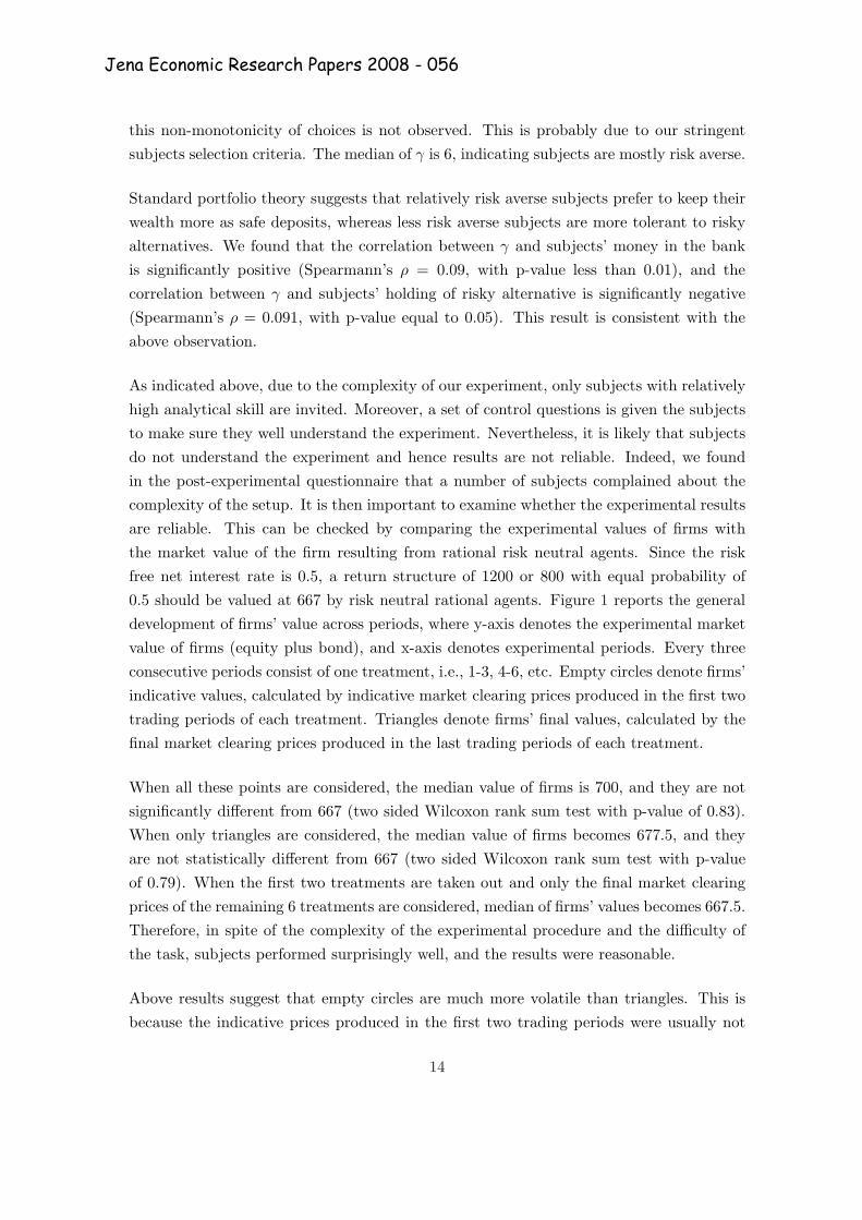
As indicated above, due to the complexity of our experiment, only subjects with relativelyhigh analytical skill are invited. Moreover, a set of control questions is given the subjectsto make sure they well understand the experiment. Nevertheless, it is likely that subjectsdo not understand the experiment and hence results are not reliable. Indeed, we foundin the post-experimental questionnaire that a number of subjects complained about thecomplexity of the setup. It is then important to examine whether the experimental resultsare reliable. This can be checked by comparing the experimental values of firms withthe market value of the firm resulting from rational risk neutral agents. Since the riskfree net interest rate is 0.5, a return structure of 1200 or 800 with equal probability of0.5 should be valued at 667 by risk neutral rational agents. Figure 1 reports the generaldevelopment of firms’ value across periods, where y-axis denotes the experimental marketvalue of firms (equity plus bond), and x-axis denotes experimental periods. Every threeconsecutive periods consist of one treatment, i.e., 1-3, 4-6, etc. Empty circles denote firms’indicative values, calculated by indicative market clearing prices produced in the first twotrading periods of each treatment. Triangles denote firms’ final values, calculated by thefinal market clearing prices produced in the last trading periods of each treatment.

When all these points are considered, the median value of firms is 700, and they are notsignificantly different from 667 (two sided Wilcoxon rank sum test with p-value of 0.83).When only triangles are considered, the median value of firms becomes 677.5, and theyare not statistically different from 667 (two sided Wilcoxon rank sum test with p-valueof 0.79). When the first two treatments are taken out and only the final market clearingprices of the remaining 6 treatments are considered, median of firms’ values becomes 667.5.Therefore, in spite of the complexity of the experimental procedure and the difficulty ofthe task, subjects performed surprisingly well, and the results were reasonable.

Above results suggest that empty circles are much more volatile than triangles. This isbecause the indicative prices produced in the first two trading periods were usually not

14


5 10 15 20

500

600

700

800

900

1000

1100

1200

Periods

Valu

e of

firm

s

Figure 1: Values of firms across periods

mature yet. Moreover, since these prices were not real market clearing prices, subjectsmight not submit their formal orders during this time, rather, they might either take thisopportunity to understand the market mechanism or to enter deceptive orders in the hopeof fooling others.

Indeed, it seems there are two levels of learning happening in this phase of the experiment.The first level of learning occurs within each treatment. This is confirmed when comparingindicative prices with final market clearing prices (respectively empty circles and trianglesin figure 1). It is found that the mean of firms’ values is closer to 667 when only finalmarket prices are considered (the mean of firms’ values based on indicative prices is 715.90;whereas the mean of firms’ values based on final market clearing prices is 692.55). Wealso performed a non-parametric variance ratio test (Gibbons and Chakraborti, 1993) tocompare the variance of indicative prices and final market clearing prices. We find thatindicative prices are significantly more volatile than final market clearing prices (one sidedrank based Ansari-Bradley two sample test, p < 0.01), possibly a result of learning.

In order to examine the second level of learning: learning across periods, the developmentof firms’ values across periods is examined. Before presenting the statistic model andresults, however, an additional feature of the experiment needs to be considered. In the

15


Table 1: Regression results

Regressions Variable Coefficient Std. Error t-statistic p-valueAll treatments υ 735.9663** 25.8236 28.4997 0.0000

t -3.7310* 1.5191 -2.4562 0.0169Last 7 treatments υ 690.4385** 23.6855 29.1502 0.0000

t -1.2017 1.3008 -0.9238 0.3598** Significant at p = 0.01, * Significant at p = 0.05.

experiment, firms are valued independently within groups, thus firms’ values criticallydepend on groups’ composition of risk attitudes. A group with relatively less risk aversesubjects tends to evaluate a firm higher than a group with relatively more risk aversesubjects, and this difference can be significant. Indeed, the standard deviation of themeans of groups’ firms’ values is as large as 47.08. Hence, a good statistic model shouldtake group heterogeneity into account and have proper control of it. For this purpose, werun a linear regression with mixed effects5 based only on final market clearing prices, wherethe dependent variable is firms’ values, independent variables are intercept and period (t),and random effects that vary across 9 groups are the intercept. Since, as suggested above,subjects’ behaviors in the first treatment are very volatile, a similar regression is run basedonly on the last 7 treatments. Formally, the model is as follows:

Vi = υ + ui + α · t + εi, (12)

where i ∈ {1, 2, . . . , 9} denotes the 9 independent groups, ui v N(0, σ2u) denotes the

random effects in the intercept for each group, and εi v N(0, σ2e). Results of regression

are presented in table 1.

When all treatments are considered, the coefficient for period turns out to be weaklysignificant (−3.7310 with p < 0.05), indicating that firms’ values decrease across periodsand approach to 667. However, when only the last 7 treatments are considered, thiscoefficient is not significant anymore, indicating that learning mainly occurs in the firsttreatment. Since we are mainly interested in the equilibrium behavior, this result suggeststhat, due to learning and non-binding of indicative prices, indicative prices in the first twotrading periods of each treatment are not mature yet, and the final market clearing pricesin the first treatment are too volatile to be used. Therefore, following statistical analysiswill mainly rely on final market clearing prices of the last 7 treatments, unless explicitlystated otherwise.

5See Jose C. Pinheiro (1993) for a good reference of mixed effects models.

16


0 100 200 300 400 500

600

700

800

900

1000

1100

1200

The value of the bond

The

val

ue o

f the

firm

Figure 2: Firms’ value conditional on the market value of bonds

4.2 The main hypothesis

We now turn to our main hypothesis: does capital structure affect the value of the firm,and if so, how?

In the theory of the cost of capital, there are mainly two competing ones: the Modigliani-Miller theorem and the U shape cost of capital. The Modigliani-Miller theorem statesthat the value of the firm is independent of the capital structure; whereas the U shapecost of capital implies that the cost of capital first decreases with the value of bond, andthen increases after the ratio of bonds exceeds some threshold. In the following, we shallcompare these two theories and see which best organizes data.

Figure 2 reports the value of the firm as a function of the value of bond for all 9 groups.All prices are used in order to give a general picture.

As before, empty circles denote values of firms based on indicative prices, and trianglesdenote values of firms based on final market clearing prices. The horizontal line is V = 667,the value of firms implied by risk neutral rational agents. Visually, it seems the horizontalline captures data quite well.

17


0 100 200 300 400 500

500

700

900

1100

Group 1


The

val

ue o

f the

firm

0 100 200 300 400 500

500

700

900

1100

Group 2


The

val

ue o

f the

firm

0 100 200 300 400 500

500

700

900

1100

Group 3


The

val

ue o

f the

firm

0 100 200 300 400 500

500

700

900

1100

Group 4


The

val

ue o

f the

firm

0 100 200 300 400 500

500

700

900

1100

Group 5

The value of the bondT

he v

alue

of t

he fi

rm0 100 200 300 400 500

500

700

900

1100

Group 6


The

val

ue o

f the

firm

0 100 200 300 400 500

500

700

900

1100

Group 7


The

val

ue o

f the

firm

0 100 200 300 400 500

500

700

900

1100

Group 8


The

val

ue o

f the

firm

0 100 200 300 400 500

500

700

900

1100

Group 9


The

val

ue o

f the

firm

Figure 3: The value of the firm conditional on the value of the bond for the 9 groups

As mentioned above, group heterogeneities might blur the picture, in figure 3, we reportthe same relationship for each group. Here, the horizontal real line denotes the group meanof firms’ values when only final market clearing prices are considered, and the horizontalvirtual line is V = 667.

The Modigliani-Miller theorem suggests that the increase of leverage increases the sys-tematic risk of equity. How well did our experimental subjects recognize the change ofsystematic risk due to the change of the capital structure? For this purpose, we computethe correlation between the value of the equity and the value of bond. This correlationis negative and close to −1 (Spearman’s ρ = −0.9313, p < 0.01. First treatment is ex-cluded, and only the final market clearing prices are considered). Thus, it seems thechange of systematic risk could be almost perfectly recognized, a result consistent withthe Modigliani-Miller theorem.

To examine the relationship between the value of the firm and the value of the bond moreprecisely, we run a linear regression with mixed effects. The first treatment are excludedand only the final market clearing prices are used. Explanatory variables are the intercept(υ), the value of bond (B), the square of the value of bond (B2), and period (t). Random

18



Expl. Variable Coefficient Std. Error t-statistic p-valueυ 654.1631** 25.566248 25.5870 0.0000B 0.4846** 0.1568 3.0900 0.0032B2 -0.0009** 0.0003 -2.9071 0.0054t -1.6570 1.3129 -1.2621 0.2127Std. dev. of the random effects σu = 33.8011;

Std. dev. of the error term σe = 57.9559** Significant at p = 0.01.

effects are the 9 independent groups. Formally, the model is as follows:

Vi = υ + ui + β1 ·Bi + β2 ·B2i + β3 · t + εi, (13)


random effects in the intercept for each group, and εi v N(0, σ2e). The results of the

regression are presented in Table 2.

As we can see from tale 2, both coefficients for B and B2 are statistically significant.Moreover, the signs of these two coefficients are consistent with the U shape cost of capitalhypothesis. The coefficient for t is not significant, suggesting that, after excluding the firsttreatment, learning is not significant anymore.

Another way to look at data reveals similar information. We run a different regressionmodel with mixed effects, where the dependent variable is weighted average cost of capital(WACC), calculated as the expected return of the firm (1000) divided by the marketvalue of the firm, and independent variables are financial leverage (τ), measured as theratio of market value of debt to the market value of the firm, τ2, and period (t). Formally,the model is:

WACCi = κ + ui + β1 · τi + β2 · τ2i + β3 · t + εi, (14)


random effects in the intercept for each group, and εi v N(0, σ2e). The results of the

regression are presented in Table 3.

Both regressions are in favor of the U shape cost of capital theory. And based on aboveparameters, the weighted average cost of capital can be written as a function of leverage

19



Expl. Variable Coefficient Std. Error t-statistic p-valueκ 1.5715** 0.0552 28.4585 0.0000τ -0.8127** 0.1979 -4.1074 0.0001τ2 0.9868** 0.2380 4.1462 0.0001t 0.0024 0.0029 0.8460 0.4015Std. dev. of the random effects σu = 0.07429;

Std. dev. of the error term σe = 0.1255;Number of observations 63

** Significant at p = 0.01, * Significant at p = 0.05.

ratio:

WACC = 1.5715− 0.8127 · τ + 0.9868 · τ2. (15)

Figure 4 reports and fitted values for regression 14 and the curve implied by equation (15).

5 Conclusion

When a firm’s leverage increases, the systematic risk of the equity of the firm increasesas well. Modigliani and Miller (1958) show that the increased rate of return required byequity holders exactly offsets the lower rate of return required by bonds, and as a result, theweighted average cost of capital remains the same. In this paper, we experimentally testthe Modigliani-Miller theorem. Our experimental result suggests that subjects recognizethe increased systematic risk of equity when leverage increases, and they ask for higherrate of return for bearing this risk. Yet, this adjustment is not perfect: they underestimatethe systematic risk of low leveraged equity and overestimated the systematic risk of highleveraged equity, resulting in a U shape weighted average cost of capital.

However, we have to stress that we do not regard our results as definitive but merely asan indicative of a useful methodology, and that the evidence presented above suggeststhat the effect of capital structure to the cost of capital is not entirely clear and thusmore study should be done. After all, as suggested in numerous research in behavioraleconomics (Kahneman and Tversky, 1984; Thaler, 1993), investors are far from being aperfect “Homo economist”. Because of these “imperfections”, it is unclear whether the

20


0.0 0.2 0.4 0.6 0.8

1.4

1.5

1.6

1.7

1.8

Leverage

Wei

ghte

d av

erag

e co

st o

f cap

ital

Figure 4: Weighted average cost of capital in relation to the leverage ratio

Modigliani-Miller theorem is the only correct theory.

21


References

Economides, N. and Schwartz, R. A. (1995). Electronic call market trading. Journal ofPortfolio Management, 21:10–18.

Fischbacher, U. (1999). z-tree - experimenter’s manual. IEW - Working Papersiewwp021, Institute for Empirical Research in Economics - IEW. available athttp://ideas.repec.org/p/zur/iewwpx/021.html.

Gibbons, J. D. and Chakraborti, S., editors (1993). Nonparametric Statistical Inference(Statistics, a Series of Textbooks and Monographs). Marcel Dekker.

Hirshleifer, J. (1966). Investment deision under uncertainty: Application of the statepreference approach. Quarterly Journal of Economics, 80(2):252–277.

Holt, C. A. and Laury, S. K. (2002). Risk aversion and incentive effects in lottery choices.American Economic Review, 92:1644–1655.

Jose C. Pinheiro, D. M. B., editor (1993). Mixed Effects Models in S and S-Plus. Springer.

Kahneman, D. and Tversky, A. (1984). Choices, values, and frames. American Psycholo-gist, 39:341–350.

Lee, W. (1987). The Effect of Exhcange Offers and Stock Swaps on Equity Risk andShareholders’ Wealth: A signalling Model Approach. PhD thesis, UCLA.

Masulis, R. W. (1980). The effects of capital structure change on security prices : A studyof exchange offers. Journal of Financial Economics, 8(2):139–178.

Miller, M. H. (1988). The modigliani-miller propositions after thirty years. Journal ofEconomic Perspectives, 2(4):99–120.

Miller, M. H. and Modiglian, F. (1966). Some estimates of the cost of the capital to theelectric utility industry, 1954-57. American Economic Review, 56:333–391.

Modigliani, F. and Miller, M. H. (1958). The cost of capital, corporation finance and thetheory of investment. American Economic Review, 48(3):261–297.

Pinegar, J. M. and Lease, R. C. (1986). The impact of preferred-for-common exchangeoffers on firm value. Journal of Finance, 41(4):795–814.

Robichek, A. A., McDonald, J. G., and Higgins, R. C. (1967). Some estimates of the costof capital to electric utility industry, 1954-57: Comment. American Economic Review,57:1278–1288.

22


Shleifer, A. and Vishny, R. W. (1997). The limits of arbitrage. Journal of Finance,52:35–55.

Stiglitz, J. E. (1969). A re-examination of the modigliani-miller theorem. AmericanEconomic Review, 59(5):784–93.

Thaler, R. H., editor (1993). Advances in Behavioral Finance. Russell Sage Foundation,New York.

Weston, J. F. (1963). A test of capital propositions. Southern Economic Journal, 30:105–112.

23
