Online Continuous Stereo Extrinsic Parameter Estimation

Peter HansenComputer Science Department

Carnegie Mellon University in QatarDoha, Qatar

phansen@qatar.cmu.edu

Hatem Alismail, Peter Rander, Brett BrowningNational Robotics Engineering Center

Robotics Institute, Carnegie Mellon UniversityPittsburgh PA, USA

{halismai,rander,brettb}@cs.cmu.edu

Abstract

Stereo visual odometry and dense scene reconstructiondepend critically on accurate calibration of the extrinsic(relative) stereo camera poses. We present an algorithmfor continuous, online stereo extrinsic re-calibration oper-ating only on sparse stereo correspondences on a per-framebasis. We obtain the 5 degree of freedom extrinsic posefor each frame, with a fixed baseline, making it possible tomodel time-dependent variations. The initial extrinsic es-timates are found by minimizing epipolar errors, and arerefined via a Kalman Filter (KF). Observation covariancesare derived from the Cramer-Rao lower bound of the solu-tion uncertainty. The algorithm operates at frame rate withunoptimized Matlab code with over 1000 correspondencesper frame. We validate its performance using a variety ofreal stereo datasets and simulations.

1. IntroductionStereo vision is core to many 3D vision methods in-

cluding visual odometry and dense scene reconstruction.Good calibration, both intrinsic and extrinsic, is essentialto achieving high accuracy as it impacts image rectifica-tion, stereo correspondence search, and triangulation. In-trinsic calibration models image formation for each cam-era (e.g. [3]), while extrinsic calibration models the 6 de-gree of freedom (DOF) pose between the cameras. For realsystems, extrinsic calibration errors occur more frequentlydue to larger exposure to shock, vibration, thermal variationand cycling. For visual odometry in particular, such errorslead to biased results. We propose a method to recalibrateextrinsic parameters online to correct drift or bias. Fig. 1shows epipolar errors for a range of stereo heads. For 1band 1c there is a near constant bias, while 1a drifts possiblycaused by thermal expansion from the lighting assembly.

Online calibration remains an active area of research.Online intrinsic calibration (auto or self calibration) es-timates intrinsic parameters using scene point correspon-

dences from multiple views (e.g. [18, 17, 8, 11]). How-ever, the results are generally less accurate than offlinemethods [8] using known relative Euclidean control points(e.g. [16]). Here, we focus on correcting drifting extrin-sic calibration. Carrera et al. [2] calibrated multi-cameraextrinsics using monocular visual SLAM maps for eachcamera [6], not necessarily with overlapping fields of view.However, the extrinsic estimates were assumed to be sta-ble over time and monocular SLAM limits real-time perfor-mance in large environments. In contrast, continuous meth-ods output a unique extrinsic pose for each stereo pair (pertime step). In [1], a linear essential matrix estimate is usedto find relative pose, followed by non-linear refinement in-corporating depth ordering constraints. Some constraintswere placed on the extrinsic pose DOF, and experimentaltesting was restricted to small indoor sequences with a sta-tionary camera.

Dang et al. [5, 4] developed an approach that estimatesthe extrinsics using three error metrics incorporated intoan iterative Extended Kalman Filter (EKF). The error met-rics are derived from bundle adjustment (BA), epipolar con-straints, and trilinear constraints. Comparisons were madevia scene reconstruction accuracy, and they found that us-ing epipolar constraints (epipolar reprojection errors) onlyto be inferior to using all three metrics. The number of cor-respondences was limited (< 50), and using more is likelyto significantly impact real-time performance. Interestingly,there were several advantages to using epipolar errors only.These include the ability to obtain strictly per-frame esti-mates without needing temporal correspondences and theinvariance to non-rigid scenes, which is important for oper-ations in dynamic environments.

In this paper, we contribute a continuous, online, extrin-sic re-calibration algorithm that operates in real-time usingonly sparse stereo correspondences and no temporal con-straints. The initial extrinsic estimates are obtained by min-imizing epipolar errors, and a Kalman Filter (KF) is usedto limit over-fitting. The unique extrinsics estimated foreach stereo pair enable temporal drift to be modeled and we

1

~15deg.Polarizing

material

LEDs

~15deg.

0 2 4 6 8−1.5

−1

−0.5

0

0.5

1

Time (minutes)

Ep

ipo

lar

Err

or

(pix

els

)

(a) Pipe dataset: f = 1203pix, 1200× 768pix2 images.

0 2 4 6 8 10 12−1

−0.5

0

0.5

1

Time (minutes)

Ep

ipo

lar

Err

or

(pix

els

)

(b) Outdoor dataset 1: f = 811pix, 640× 480pix2 images.

0 2 4 6 8 10 12 14 16 18 20 22−24

−22

−20

−18

−16

−14

Time (minutes)

Ep

ipo

lar

Err

or

(pix

els

)

(c) Outdoor dataset 2: f = 1781pix, 1024×768pix2 images.

Figure 1: Mean (blue) and ±3σ standard deviation (red)epipolar errors for sparse correspondences for differentstereo data. The supplied calibration (Pointgrey Bumble-bee2) was used for rectification in (b).

show that with enough correspondences (e.g. 1000), epipo-lar errors alone are sufficient for good re-calibration. More-over, the approach is trivial to extend to multiple frames bycombining correspondences. We validate the approach insimulation and on real stereo datasets by comparing visualodometry estimates with and without re-calibration, and re-construction errors compared to offline calibration with aknown target. We show the limitations of re-calibrating thebaseline length, and suggest methods to partially addressthese.

2. Stereo Geometry and Error Metric2.1. Stereo Pose and Epipolar Constraints

The stereo extrinsics S = [R|t], is composed of a rota-tion R ∈ SO(3) and translation t ∈ R3. It defines the pro-jection of a scene point Xl = (X,Y, Z)T in the left camera,to Xr in the right: Xr = RXl + t.

Our re-calibration algorithm uses image coordinates anderrors in the left and right stereo rectified images. Let ul ↔ur be a set of homogeneous scene point correspondencesin a pair of rectified images, which are related to the scenepoints coordinates Xl,Xr by

ul ' Kl RlXl = Kl Xl (1)

ur ' Kr RrXr = Kr Xr, (2)

where Rl, Rr are rotations applied to each camera, andKl,Kr are pinhole projection matrices with zero skew andequal focal lengths f . For convenience we assume that

Kl = Kr =

f 0 uo0 f v0

0 0 1

. (3)

Rl and Rr are selected to produce a rectified extrinsic poseS = [I3×3 | (−b, 0, 0)T ], where b = ||t|| is the originalbaseline, such that Xr = Xl + (−b, 0, 0)T (e.g. [12]).

The rectified coordinates are related by

(ul, vl, 1)T = (ur + d, vr, 1)T , d =bf

Z, (4)

where d is the disparity and Z the depth of a scene point.The stereo rectified epipolar constraint is simply vl = vr,which is independent of the depth and baseline. Thiscan also be derived from the monocular essential matrixulE ur = 0 [12].

2.2. Calibration Error Metric

For re-calibration, we decompose each rotation, Rl andRr, as the product of two independent rotations:

Rl = RTl R′l, Rr = RTr R

′r. (5)

They are the rotations R′l and R′r from the original stereoextrinsics S, and a rotation correction Rl and Rr. We startwith a set of correspondences u′l ↔ u′r detected in imageryrectified with R′l and R′r. They are related to the correctrectified coordinates ul ↔ ur, satisfying the epipolar con-straint by

ul ' KlRTl K−1l u′l, ur ' KrR

Tr K−1r u′r. (6)

For an estimate of Rl and Rr, the epipolar error εi is

εi = fRTl[2]K

−1l u′li

RTl[3]K−1l u′li

− fRTr[2]K

−1r u′ri

RTr[3]K−1r u′ri

, (7)

Stereo rectification plane

Figure 2: The parameterization of the rotation angles Φ. Inthe rectified pose, the cameras principal axes are parallel,and lie in the plane Π. The rectified coordinates are pro-jected to a plane orthogonal to Π.

where RTa[b] means row b of matrix RTa . The re-calibrationobjective function is the sum of squared epipolar errors ε:

argminRl,Rr

N∑i=1

ε2i , (8)

giving the maximum likelihood estimate of Rl and Rr, fromwhich the new S stereo extrinsics can be recovered:

S = 〈Qr, Q∗l 〉, (9)

Ql =[(RTl R

′l

)T |0]→ Q∗l =[RTl R

′l|0], (10)

Qr =[(RTr R

′r

)T | (RTr R′r)T (−b, 0, 0)T], (11)

where 〈Qr, Q∗l 〉 is the projection Q∗l followed by Qr.As we can only use epipolar constraints, there is no

means for correcting the stereo baseline estimate b. Weintroduce a method to partially address this in section 4.3.We restrict the optimized extrinsic pose by 1 DOF as a re-sult and instead optimize the 5 DOF vector of Euler anglesΦ = [αl, βl, αr, βr, γ]

T by minimizing (8). Referring toFig. 2, the rotations Rl and Rr are

Rl = RX(γ/2)RZ(βl)RY (αl) (12)

Rr = RX(−γ/2)RZ(βr)RY (αr), (13)

whereRA is the right-handed rotation about the axisA. Eu-ler angles are a suitable parameterization as the initial ex-trinsic estimate is assumed to be near the solution, and theexpected changes in angles are small.

3. Solution Covariance and Over FittingIn practice, the correspondences u′l ↔ u′r will be cor-

rupted with noise and the ability to accurately estimate Φfrom these is dependent on many factors. These include: thefocal lengths, baseline, number of correspondences, spatialdistribution of correspondences, and the depth of the scenepoints. Small rotation angles Φ make over-fitting a concern.

Figure 3: Ground truth simulated change in angles Φ′ (blackline), and the initial optimized estimates Φ (red dots).

To test this, we simulated a time dependent change in theextrinsic pose of a b = 150mm baseline, 640 × 480 reso-lution (f = 1000pix) stereo camera. For each stereo pair,1000 random correspondences were generated, and uncor-related Gaussian noise (σ = 0.5pix) added. The disparityvalues ranged between 1 and 25pix, or equivalently depthsZ between 3 and 150m. Fig. 3 shows the simulated angularchanges (black), and the noisy estimates of Φ (red).

3.1. Solution Covariance

Assuming that Φ is an unbiased estimate of thesolution Φ′, with expected error covariance C =E[(Φ− Φ′) (Φ− Φ′)T

], the Cramer-Rao lower bound C is

greater than or equal to the inverse of the Fisher informationmatrix F , which is the score variance at the solution [15]:

C = E[(Φ− Φ′) (Φ− Φ′)T

]≥ F−1 (14)

F = E

[(∂ ln p(ε|Φ)

∂Φ

)T (∂ ln p(ε|Φ)

∂Φ

)]. (15)

Where p(ε|Φ) is the conditional error probability. If themeasurement errors of the imaged points are zero-meanGaussian, then we can assume that ε ∼ N (0, σ) at the solu-tion, and (15) can be written as

F =1

σ2

n∑i=1

(∂εi∂Φ

)T (∂εi∂Φ

). (16)

The summation in (16) is taken over all n correspondences,and the Jacobian ∂εi

∂Φ is the change in error with respect tothe change in parameters Φ at the solution:

Ji =[

∂εi∂αl

∂εi∂βl

∂εi∂αr

∂εi∂βl

∂εi∂γ

], (17)

which, for the simple case where Φ = 0T is

Ji|0T =[−xli

ylif −xli

xriyrif xri

f2+y2li+y2ri

2f

].

(18)

C αl βl αr βr γ

αl 0.040 0.031 -0.010 0.030 0.019βl 0.031 3.142 0.070 3.127 1.969αr -0.010 0.070 0.041 0.070 0.044βr 0.030 3.127 0.070 3.117 1.961γ 0.019 1.969 0.044 1.961 1.235

(a) Pipe dataset (see Fig. 1a). All scene points are within300mm of the camera. det(C) = 8.452× 10−42.

C αl βl αr βr γ

αl 178.414 2.562 178.884 2.737 -0.013βl 2.562 0.967 2.710 0.979 0.007αr 178.884 2.710 180.958 2.979 -0.013βr 2.737 0.979 2.979 1.002 0.007γ -0.013 0.007 -0.013 0.007 0.001

(b) Outdoor dataset 1 (see Fig. 1b). Many scene points are > 10mfrom the camera. det(C) = 4.602× 10−37.

Table 1: Covariance matrices for the correspondences in (a)Fig. 1a and (b) Fig. 1b. The units are deg2 /pix2, and allvalues have been scale by 1.0× 103 for display purposes.

From (6), (xl, yl)T = (ul − u0, vl − v0)T and (xr, yr)

T =(ur−u0, vr−v0)T . Due to its complexity we omit here thefull Jacobian. For most perspective cameras with averagefields of view the component ∂ε

∂γ dominates the magnitudeof J , suggesting that γ will be the most reliable estimate.

Table 1 shows the covariance matrices for the sets of cor-respondences in Fig. 1a and Fig. 1b. The variances of theangles (leading diagonal) differ significantly in the exam-ples, and although the number of correspondences used wassimilar, the determinant of C for the pipe example is severalorders of magnitude smaller than the outdoor 1 example.For the outdoor 1 example, the majority of the scene pointsare distant, and there is a large covariance between the α an-gles (αl and αr, highlighted in blue), as well as the β angles(βl and βr, highlighted in red)1. This shows that it is pri-marily the relative angles δα = αl − αr and δβ = βl − βrbeing estimated (see Fig. 5). For example, if points at aninfinite distance are observed in a perfectly rectified stereopair, such that u′l = u′r, the epipolar errors

∑ε2i will be

zero for any rotations where βl = βr (δβ = 0). In effectthis is attempting to estimate a small translation using pointsat infinity (Fig. 4). It is only when βl 6= βr that

∑ε2i > 0.

4. Kalman Filter Re-Calibration

Given the noisy estimates Φ of the extrinsic pose ob-tained from the non-linear minimization of the epipolar er-rors, we use a KF [13] to produce a smoothed estimate Φ.We use a stationary process model so that we have at time kΦk = Φk−1, although more complex models could be used.

1For any point at infinity, u′l = u′r , so ∂ε∂αl

= ∂ε∂αr

and ∂ε∂βl

= ∂ε∂βr

.

Figure 4: For a point at infinity, only relative angles can beestimated, for example δβ = βl−βr. Rotating the camerasby the same angle βl = βr (δb = 0) is approximately equiv-alent to adding a small translation change δt, and estimatingsmall translations with distal points is problematic.

The lower bound Ck evaluated at time k is used as the mea-surement noise covariance. The process noise covarianceQis set to

Q =( π

180

)2(

τ

60× fps

)2

Diag(1, 1, 1, 1, 0.25), (19)

where fps is frames per second, and τ is the selected angu-lar rate of the process noise with units of degrees per minute.

4.1. Update Equations

The time update predictions for the camera state Φ−k , er-ror covariance P−k , and Kalman gain Kk are

Φ−k = Φk−1 (20)

P−k = Pk−1 +Q (21)

Kk = P−k(P−k + Ck

)−1, (22)

from which the updated estimate of the camera state Φk anderror covariance Pk are evaluated as

Φk = Φ−k +Kk(

Φ− Φ−k

)(23)

Pk = (I5×5 −Kk)P−k . (24)

4.2. Initializing the State Covariance

We estimate the initial state covariance Pk=0 by gener-ating 50 perfectly rectified frames of checkerboard scenepoints (120 points per frame). Random poses of the cam-eras with respect to the checkerboard target are simulated.Gaussian noise is then added to each image coordinate withσ = 0.25pix. The reprojection errors are defined as a func-tion of the Euler angles (6) — the y error component is(7). The initial estimate Pk=0 is calculated from the lowerbound of the solution uncertainty.

Figure 5 shows the KF results Φ obtained from the orig-inal optimized estimates Φ in the example in Fig. 3 usingthe process noise rate τ = 1e−3. It is clear from Fig. 5 thatthe KF estimates of the individual angles αl, αr, βl, βr donot accurately estimate the simulated angles. However, thedifferential angles δα = αl − αr and δβ = βl − βr shownin the same figure are close approximations of the simulateddifferential angles. Note that γ is also a differential angle,and its filter estimate is very close to the simulated values.

0 4500−0.05

0

0.05

0.1

0.15

Frame

αl (

deg)

0 4500−0.05

0

0.05

0.1

0.15

Frameα

r (deg)

0 4500−0.05

0

0.05

0.1

Frame

αl−α

r (deg)

0 4500−0.15

−0.1

−0.05

0

0.05

Frame

βl (

deg)

0 4500−0.15

−0.1

−0.05

0

0.05

Frame

βr (

deg)

0 4500−0.1

−0.05

0

0.05

Frame

βl −

βr (

deg)

0 4500−0.05

0

0.05

0.1

0.15

Frame

γ (d

eg)

Figure 5: Ground truth angles Φ (black) and KF estimates Φ(red) – original estimates Φ shown in Fig. 3. The differentialangles δα = αl − αr, δβ = βl − βr are also shown.

4.3. Baseline Estimation

The true baseline distance cannot be measured fromstereo correspondences, however, it may be estimated usingadditional information. Examples include inertial or wheelodometry, fixed reference fiduciary markers, or structuredlight measurement observable in both images. Here, weused the following per-frame method to obtain the results insection 5. We assume that triangulated distance to a scenepoint Xi should be the same using both the original and re-calibrated extrinsics. We denote these li and l′i, respectively.Since distances are proportional to the triangulated depths(see 4), we estimate the new baseline b as

b =b

n

n∑i=1

lil′i. (25)

The summation is only taken over the nearest n = 5 stereocorrespondences each frame as the nearest points are themost suitable for resolving translation magnitudes.

5. Experiments and ResultsTo evaluate the approach, we present a range of experi-

mental online re-calibration results including visual odom-etry for the datasets in Fig. 1 (see table 2), and scene recon-struction using the dataset described in Sect. 5.

For all datasets, Harris corners [10] were detected inimage pairs rectified using the original extrinsics. Sparsestereo correspondences were found by thresholding the co-sine similarity between SIFT descriptors [14] for each fea-ture. Although sub-pixel accuracy Harris corners werefound, Zero-Normalized Cross Correlation (ZNCC) wasused to refine the correspondences and improve accuracy.

Pipe Outoor 1 Outdoor 2Camera Assembled Commercial Assembled

Resolution 1202x768 640x480 1033x768#images 971 8278 7567

fps 7.5 15 7.5f (pix) 1203 811 1781b (mm) 156 120 342# stereo 1236 947 885

Length (m) 7.1 5477 6247

Table 2: Summary of the visual odometry datasets (see alsoFig. 1). The notation # stereo is the mean number of stereocorrespondences found per frame. The camera parametersare given for the stereo rectified images.

Importantly, we constrain the right stereo feature to anepipolar box and not a line.

For the visual odometry results, temporal correspon-dences between adjacent stereo pairs were found by thresh-olding the ambiguity ratio [14] between SIFT descrip-tors. Visual odometry estimates were computed usingboth the original and the re-calibrated stereo extrinsic pose.The 6 DOF change in pose Q between the left cameraframes was estimated using Perspective-n-Points (PnP) andRANSAC [7], followed by non-linear minimization of theimage reprojection errors. The KF process noise was set toτ = 0.001 for each dataset, and Pk=0 estimated using themethod in Sect. 4.2.

Pipe Dataset The stereo camera, original epipolar errors,and sample rectified imagery for the pipe dataset are shownin Fig.1a. As described in [9], the camera observed the up-per surface of a 400mm diameter steel pipe as it movedforwards and then in reverse through the pipe. Light-ing via nine LEDs was mounted to the camera housing,which raised the temperature of the camera housing from25 − 30oC ambient at the start to 27 − 38oC at the end.We attribute the time dependent change in epipolar errors tothermal expansion.

The KF estimates of the camera rotation angles, visualodometry estimates, and 3D point clouds with original andre-calibration extrinsics are shown in Fig.6a, 6b, and 6c.Although GPS ground truth is unavailable, all scene pointsbelong to the same curved surface, so the reconstructions inboth directions should align. There is a large misalignmentusing the original extrinsic calibration, which is improvedsignificantly using the online re-calibration estimates.

Outdoor Dataset (Camera 1) The first outdoor dataset(Fig.1b) includes imagery from a short baseline PointgreyBumblebee2 stereo camera. The rectified imagery was cre-ated using the supplied calibration data. The KF estimatesof the extrinsics are provided in Fig.7a, and the compari-

0 2 4 6 8−0.125

−0.1

−0.075

−0.05

−0.025

0

0.025

Time (minutes)

δα

(deg)

0 2 4 6 8−0.01

−0.005

0

0.005

0.01

0.015

Time (minutes)

δβ (

deg)

0 2 4 6 8−0.25

−0.2

−0.15

−0.1

−0.05

0

0.05

0.1

0.15

Time (minutes)

γ (d

eg)

0 2 4 6 8−0.075

−0.05

−0.025

0

0.025

0.05

Time (minutes)

Angle

(deg)

(a) KF estimates of the rotations angles.

(b) VO result with pipe axis in X direction: original (top) andre-calibrated (bottom).

(c) VO result at the start/end: original (left) and re-calibrated (right).The points all belong to the same surface.

Figure 6: Results for the pipe dataset. The black line nearthe surface points in (c) connects the same ground truthmarker, reconstructed at the start and end of the dataset.The Euclidean errors in the reconstructed coordinate are:100.1mm for original calibration, 15.1mm for re-calibrated.

son of the visual odometry estimates using the original andre-calibrated extrinsic pose are shown in Fig.7b. The 5HzGPS (non-RTK) measurements collected are included asground truth. The visual odometry position estimates werelinearly interpolated at the time stamps for each of the 1671GPS readings2, and then aligned with the GPS by minimiz-ing the sum of squared distances. The average absolute dis-tance errors were: 0.781m using the original calibration,and 0.485m using online re-calibration.

2The GPS z-component was set to zero as the 3D solution was unreli-able – the operating environment was approximately planar.

0 2 4 6 8 10 12−0.4

−0.2

0

0.2

0.4

Time (minutes)

δα

(deg)

0 2 4 6 8 10 12

0

0.02

0.04

Time (minutes)

δβ (

deg)

0 2 4 6 8 10 12−0.025

−0.02

−0.015

−0.01

−0.005

0

Time (minutes)

γ (d

eg)

0 2 4 6 8 10 12−0.02

−0.01

0

0.01

0.02

0.03

0.04

0.05

0.06

Time (minutes)

Angle

(deg)

(a) KF estimates of the rotations angles.

(b) VO (red), and the 5Hz GPS (blue). Left column is the originalcalibration, and right column the KF re-calibration.

Figure 7: Results for 5.48km outdoor dataset 1 (commercialstereo camera). There are a total of 4 anti-clockwise loops.

Outdoor Dataset (Camera 2) The second outdoordataset (see Fig.1c) uses a custom 342mm baseline stereocamera. Intrinsic and extrinsic parameters were calibratedoffline and then we manually flexed the camera to alter theextrinsics. The KF estimates of the angles and visual odom-etry results are provided in Fig.8. GPS ( 3045 points at5Hz) formed the ground truth using the same techniquesdescribed previously. The absolute average distance errorswere: 1.632m using the original calibration, and 0.700musing online re-calibration. As was the case with the firstoutdoor dataset, re-calibration reduced the rotational drift.

Indoor Scene Fig. 9a shows the stereo camera and a sam-ple image from the left camera used for the indoor con-trolled test. The stereo head uses the same cameras as in theprevious experiment, but with a baseline of 220mm and aconfigurable right camera pose. We collected three datasets

(a) KF estimates of the rotations angles.

(b) VO (red), and the 5Hz GPS (blue). Left column is the origi-nal calibration, and right column the KF re-calibration.

Figure 8: Results for 6.25km outdoor dataset 2.

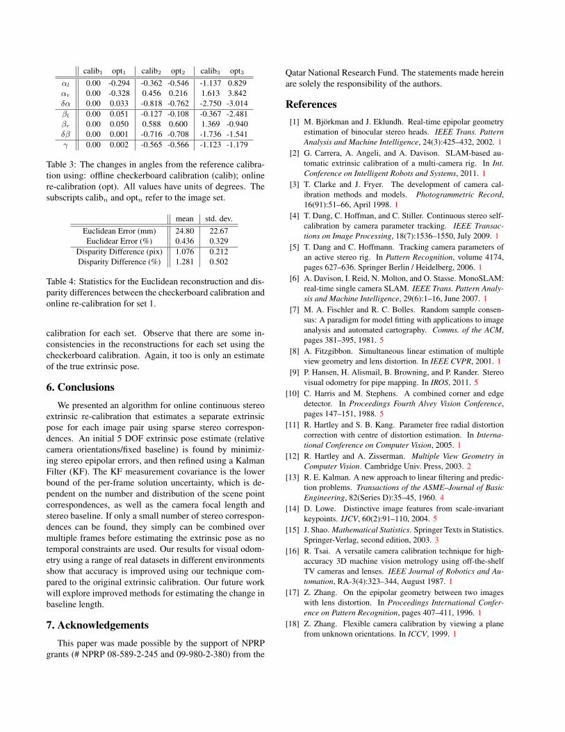
(1, 2 and 3) observing the same indoor scene, each with adifferent right camera pose. Ground truth estimates of theextrinsic pose for each set were obtained using a checker-board target. Dataset 1 was chosen as the reference calibra-tion. The stereo correspondences for each set were foundin rectified imagery using this reference calibration. Theonline KF re-calibration was used to estimate the changesfrom the reference calibration, as shown in Fig. 9b. Thefinal KF results are compared to the ground truth in table 3.

As expected, the performance degrades with largechanges from the reference calibration. Although the errorsfor αl and αr appear large for set 1, the resulting change inthe stereo disparity and scene reconstruction remained rel-atively small (see table 3). The standard deviation of thedisparity (pix) is similar to the checkerboard calibration re-projection values of (σx, σy) = (0.231, 0.212)pix which isitself only an estimate of the true extrinsic pose.

To better visualize the performance of the re-calibration,the overhead views of the scene reconstruction for each

(a) The stereo camera and sample image.

δ α

0 100 200−0.1

−0.05

0

0.05

0.1

δ β

0 100 200−0.1

−0.05

0

0.05

0.1

γ

0 100 200−0.1

−0.05

0

0.05

0.1

0 200 400−1

−0.75

−0.5

−0.25

0

de

gre

es

0 200 400−1

−0.75

−0.5

−0.25

0

0 200 400−1

−0.75

−0.5

−0.25

0

0 100 200 300

−3.9

−2.9

−1.9

−0.9

0 100 200 300−2.5

−2

−1.5

−1

−0.5

0

Frame0 100 200 300

−2

−1.5

−1

−0.5

0

(b) The raw online calibration angle estimates (red points) and KF estimates(solid lines). Each row shows the differential angle estimates for each of the3 datasets (changing right camera pose).

0 10 20 30−6

−4.5

−3

−1.5

0

1.5

Y (

me

ters

)

0 2 4 6 8−0.5

0

0.5

1

Y (

me

ters

)

0 2 4 6 8−0.5

0

0.5

1

Z (meters)

Y (

me

ters

)

(c) The top view of the scene reconstructions for set 1 (blue), set 2 (red) andset 3 (green) using: original calibration (top row); checkerboard calibration(middle row); online KF re-calibration (bottom row).

Figure 9: Hardware and results for the indoor dataset.

set are shown in Fig. 9c: the first row uses the referencecalibration for each set; the second row uses the checker-board calibration; and the third row uses the online re-calibration. These reconstructions were produced using theexact same stereo correspondences detected in a single im-age pair from each set, and are all in the left camera co-ordinate frame. The results using online re-calibration aresignificantly more consistent than those using the reference

calib1 opt1 calib2 opt2 calib3 opt3αl 0.00 -0.294 -0.362 -0.546 -1.137 0.829αr 0.00 -0.328 0.456 0.216 1.613 3.842δα 0.00 0.033 -0.818 -0.762 -2.750 -3.014βl 0.00 0.051 -0.127 -0.108 -0.367 -2.481βr 0.00 0.050 0.588 0.600 1.369 -0.940δβ 0.00 0.001 -0.716 -0.708 -1.736 -1.541γ 0.00 0.002 -0.565 -0.566 -1.123 -1.179

Table 3: The changes in angles from the reference calibra-tion using: offline checkerboard calibration (calib); onlinere-calibration (opt). All values have units of degrees. Thesubscripts calibn and optn refer to the image set.

mean std. dev.Euclidean Error (mm) 24.80 22.67Euclidear Error (%) 0.436 0.329

Disparity Difference (pix) 1.076 0.212Disparity Difference (%) 1.281 0.502

Table 4: Statistics for the Euclidean reconstruction and dis-parity differences between the checkerboard calibration andonline re-calibration for set 1.

calibration for each set. Observe that there are some in-consistencies in the reconstructions for each set using thecheckerboard calibration. Again, it too is only an estimateof the true extrinsic pose.

6. ConclusionsWe presented an algorithm for online continuous stereo

extrinsic re-calibration that estimates a separate extrinsicpose for each image pair using sparse stereo correspon-dences. An initial 5 DOF extrinsic pose estimate (relativecamera orientations/fixed baseline) is found by minimiz-ing stereo epipolar errors, and then refined using a KalmanFilter (KF). The KF measurement covariance is the lowerbound of the per-frame solution uncertainty, which is de-pendent on the number and distribution of the scene pointcorrespondences, as well as the camera focal length andstereo baseline. If only a small number of stereo correspon-dences can be found, they simply can be combined overmultiple frames before estimating the extrinsic pose as notemporal constraints are used. Our results for visual odom-etry using a range of real datasets in different environmentsshow that accuracy is improved using our technique com-pared to the original extrinsic calibration. Our future workwill explore improved methods for estimating the change inbaseline length.

7. AcknowledgementsThis paper was made possible by the support of NPRP

grants (# NPRP 08-589-2-245 and 09-980-2-380) from the

Qatar National Research Fund. The statements made hereinare solely the responsibility of the authors.

References[1] M. Bjorkman and J. Eklundh. Real-time epipolar geometry

estimation of binocular stereo heads. IEEE Trans. PatternAnalysis and Machine Intelligence, 24(3):425–432, 2002. 1

[2] G. Carrera, A. Angeli, and A. Davison. SLAM-based au-tomatic extrinsic calibration of a multi-camera rig. In Int.Conference on Intelligent Robots and Systems, 2011. 1

[3] T. Clarke and J. Fryer. The development of camera cal-ibration methods and models. Photogrammetric Record,16(91):51–66, April 1998. 1

[4] T. Dang, C. Hoffman, and C. Stiller. Continuous stereo self-calibration by camera parameter tracking. IEEE Transac-tions on Image Processing, 18(7):1536–1550, July 2009. 1

[5] T. Dang and C. Hoffmann. Tracking camera parameters ofan active stereo rig. In Pattern Recognition, volume 4174,pages 627–636. Springer Berlin / Heidelberg, 2006. 1

[6] A. Davison, I. Reid, N. Molton, and O. Stasse. MonoSLAM:real-time single camera SLAM. IEEE Trans. Pattern Analy-sis and Machine Intelligence, 29(6):1–16, June 2007. 1

[7] M. A. Fischler and R. C. Bolles. Random sample consen-sus: A paradigm for model fitting with applications to imageanalysis and automated cartography. Comms. of the ACM,pages 381–395, 1981. 5

[8] A. Fitzgibbon. Simultaneous linear estimation of multipleview geometry and lens distortion. In IEEE CVPR, 2001. 1

[9] P. Hansen, H. Alismail, B. Browning, and P. Rander. Stereovisual odometry for pipe mapping. In IROS, 2011. 5

[10] C. Harris and M. Stephens. A combined corner and edgedetector. In Proceedings Fourth Alvey Vision Conference,pages 147–151, 1988. 5

[11] R. Hartley and S. B. Kang. Parameter free radial distortioncorrection with centre of distortion estimation. In Interna-tional Conference on Computer Vision, 2005. 1

[12] R. Hartley and A. Zisserman. Multiple View Geometry inComputer Vision. Cambridge Univ. Press, 2003. 2

[13] R. E. Kalman. A new approach to linear filtering and predic-tion problems. Transactions of the ASME–Journal of BasicEngineering, 82(Series D):35–45, 1960. 4

[14] D. Lowe. Distinctive image features from scale-invariantkeypoints. IJCV, 60(2):91–110, 2004. 5

[15] J. Shao. Mathematical Statistics. Springer Texts in Statistics.Springer-Verlag, second edition, 2003. 3

[16] R. Tsai. A versatile camera calibration technique for high-accuracy 3D machine vision metrology using off-the-shelfTV cameras and lenses. IEEE Journal of Robotics and Au-tomation, RA-3(4):323–344, August 1987. 1

[17] Z. Zhang. On the epipolar geometry between two imageswith lens distortion. In Proceedings International Confer-ence on Pattern Recognition, pages 407–411, 1996. 1

[18] Z. Zhang. Flexible camera calibration by viewing a planefrom unknown orientations. In ICCV, 1999. 1