online ev scheduling algorithms for adaptive charging

Online EV Scheduling Algorithms for Adaptive Charging Networks with Global Peak Constraints

Journal: Transactions on Sustainable Computing

Manuscript ID TSUSC-2018-12-0140.R1

Manuscript Types: Special Issue on Intersection of Computing and Communication Technologies with Energy Systems

Keywords: Electric vehicles, online scheduling, approximation algorithm, competitive analysis

https://mc.manuscriptcentral.com/tsusc-cs

Transactions on Sustainable Computing

1

Online EV Scheduling Algorithms for AdaptiveCharging Networks with Global Peak Constraints

Bahram Alinia, Mohammad H. Hajiesmaili, Zachary J. Lee, Noel Crespi, and Enrique Mallada

Abstract—This paper tackles online scheduling of electricvehicles (EVs) in an adaptive charging network (ACN) withlocal and global peak constraints. Given the aggregate chargingdemand of the EVs and the peak constraints of the ACN, itmight be infeasible to fully charge all the EVs according totheir charging demand. Two alternatives in such resource-limitedscenarios are to maximize the social welfare by partially chargingthe EVs (fractional model) or selecting a subset of EVs andfully charge them (integral model). The critical challenge is theneed for online solution design since in practical scenarios thescheduler has no information of future arrivals of EVs in a time-coupled underlying problem. For the fractional model, we deviseboth offline and online algorithms. We prove that the offlinealgorithm is optimal. Using competitive ratio as the performancemeasure, we prove the online algorithm achieves a competitiveratio of 2. The integral model, however, is more challenging sincethe underlying problem is strongly NP-hard due to 0/1 selectioncriteria of EVs. Hence, efficient solution design is challengingeven in offline setting. We devise a low-complexity primal-dualscheduling algorithm that achieves a bounded approximationratio. Built upon the offline approximate algorithm, we proposean online algorithm and analyze its competitive ratio in specialcases. Extensive trace-driven experimental results show that theperformance of the proposed online algorithms is close to theoffline optimum, and outperform the existing solutions.

Index Terms—Electric Vehicle, Online Scheduling, Approxima-tion Algorithm, Competitive Analysis

I. INTRODUCTION

TO promote quick adoption of renewable energy sources,electrification of vehicles is a trend that has been globally

advocated in recent years. According to a Bloomberg report,EVs will account for more than half of the new car sales by2040 [1]. Consequently, it is expected that demand from EVcharging will constitute a considerable portion of total demand.Currently, transportation consumes 29% of total energy in theUS, while electricity production consumes 40% [2].

EV charging demand is a typical example of a deferrableload, and there is often considerable flexibility in the chargingschedule. This property makes the problem of EV chargingscheduling important and there is an extensive research alongthis direction in the literature (see the recent survey [3], andreferences therein). In most of the existing works, the EVcharging demand is treated as a constraint to the problem

B. Alinia and N. Crespi are with the department of Networksand Mobile Multimedia Services (RS2M), Institut Mines-Telecom, Tele-com SudParis, Evry, France (e-mail: [email protected],[email protected]).

M. H. Hajiesmaili and E. Mallada are with the Department of Electricaland Computer Engineering, Johns Hopkins University, Baltimore, MD, USA(e-mail: {hajiesmaili,mallada}@jhu.edu).

Z. J. Lee is with the Department of Electrical Engineering, CaliforniaInstitute of Technology, Pasadena, CA, USA (e-mail: [email protected]).

in a low-load regime [4]. Motivated by rapid proliferation ofEVs, this work tackles the EV scheduling in high-load regime,where given the aggregate charging demand of the EVs andthe peak constraints of the charging network, it is not feasibleto fully charge all the EVs according to their charging demand.

More specifically, this paper studies resource-constrainedEV charging scheduling in an adaptive charging network(ACN) governed by a single operator in a campus-scalelocation such as a university, a headquarters, etc. [5]. A notableexample is the Caltech ACN [6] where individual chargingports are organized into several charging stations (CSs) whichare dispersed in a charging network with the capability ofadaptive charging of the EVs. The problem is different fromEV charging scheduling with capacity constraint in singlestation scenarios [2], [4], [7]–[12] (we refer to Section II fordetailed discussions on related work), because of the essentialneed to respect the aggregate peak demand of the ACN. Notethat, the ACN operator might limit the total power drawn fromEVs to control costs [13], [14], reserve the capacity for otherloads, and/or participate in demand-response programs.

We consider a scenario with multiple EVs where each EVhas different charging profile in terms of availability, chargingdemand, charging rate limit, and valuation of getting charged(for details see Section III-A2). We formulate an online EVcharging scheduling problem with the goal of selecting andscheduling a subset of EVs such that: (1) the charging demandof the selected EVs are (fully or partially) satisfied; (2) thecharging rate limit of EV batteries are respected, (3) the globalpeak constraint of the ACN is satisfied [6]; (4) the local peakconstraint of each CS is respected; and finally, (5) the totalrevenue obtained by the valuation of the EVs is maximized.

There are two main challenges in the design and imple-mentation of scheduling algorithms for EVs satisfying thegoals mentioned above. Firstly, the problem calls for onlinescheduling design. In practice, EVs arrive to the CS in onlinefashion and the scheduler has no information about the arrivaland demand of the future EVs. Secondly, the underlyingoptimization problem in integral model is strongly NP-hardeven in offline case (see Section V). This is because theproblem is a mixed integer linear problem and a “time-expanded” extension of knapsack problem which is knownas a classic NP-hard problem. In this paper, we tackle thechallenge of online design by following competitive algorithmdesign [15] and the challenge of NP-hardness by pursuingapproximation algorithm design [16] and make the followingcontributions:B We first consider a fractional model (where EVs can

be charged partially and the revenue is proportional accord-

Page 1 of 23



123456789101112131415161718192021222324252627282930313233343536373839404142434445464748495051525354555657585960

2

ingly) and design an optimal offline scheduling algorithm.We then develop an efficient online algorithm in which noexact or stochastic information about the future EV arrivalsis given. Despite its simplicity, the algorithm is proved to be2-competitive with optimal offline solution, i.e., the revenueof the proposed online algorithm is at least 1/2 of the offlineoptimum, regardless of input sequence. Even though there arecompetitive algorithms in the literature for similar problems,to the best of our knowledge, our algorithm is the first 2-competitive algorithm which considers the charging rate limits.

B We next study the more challenging scenario of theintegral model, where EVs must receive all their demand tomake revenue. We first propose a polynomial-time primal-dualoffline approximate algorithm. We analyze the approximationratio of the algorithm and by strengthening the linear relaxedversion of the mixed integer problem [17], we obtain anapproximation ratio of α = 1 +

∑mj=1

pj

pj−qj .s

s−1 , where pj islocal peak constraint in station j, qj is the maximum chargingrate of the EVs in station j and s is a slackness parameter.We highlight that when pj � qj and s is large enough, thenα ≈ m + 1, where m is the number of stations in the ACN.Built on the basis of the offline algorithm, we devise an onlinealgorithm, and discuss its competitive ratio in special cases.

B We conduct a set of simulations to evaluate the per-formance of our proposed algorithms. The results of onlinealgorithms for both integral and fractional settings are closeto the optimum (within 90% and 94% for integral and frac-tional models in a representative scenario). In addition, ouralgorithm outperforms the existing scheduling algorithm inCaltech ACN [6] by 35% for integral revenue model.

This paper represents follow-up work to our previousstudy [40], where we address a simplified version of theproblems studied in this paper in fractional revenue model. Thecompetitive analysis in [40] is done under the assumption thatall EVs have the same maximum charging rate. Also, [40] doesnot study the integral revenue model. In this paper, we extendthe results and propose a 2-competitive online algorithm withno assumption on the input parameters. Also, the currentstudy investigates both fractional and integral revenue modelswhile considering global peak constraint in the formulationand addressing multiple charging station scenario. Last, weconsider more realistic trace-driven experiments in this paperand compare the results to an existing real-world schedulingalgorithm.

II. RELATED WORK

There is an extensive work in the general topic of EV de-mand management and scheduling [3] by considering differentscenarios such as optimal operations with EV coordinationand congestion management [18], [46], [47], EV schedulingwith incorporation of renewable energy, and energy storagesystems [19], [20], and pricing and bidding [45], [48] In thissection, we focus on the literature related to peak-constrainedEV charging scheduling in single and multiple stations.

1) Peak-Constrained EV Charging Scheduling: There isan extensive literature on EV charging scheduling problemfocusing on single CS [4], [7], while the local and global peakconstraints are omitted or only the local peak is considered.

As we discuss in Section III-B, the global optimal solutioncannot be obtained by separately solving the single stationproblems. Hence, those solutions cannot be directly appliedto the multiple CS scenario with global peak constraints.

Studies in [21]–[26] tackled charging scheduling problem inmultiple CSs. The authors in [21] studied a global cost min-imization EV charging scheduling problem. However, thereis no limit on the maximum peak demand that the systemcan tolerate. Consequently, the peak can be arbitrary high andbeyond the physical limit of the transformers in the chargingstation [6] leading to huge electricity bills [14]. Besides, thecharger devices installed in the CSs have limitation on themaximum power that they can transfer in each time unit [27].[24] considered a multi-microgrid system with global peakconstraint where each microgrid has a CS and the goal isto manage electricity exchange between microgrids and maingrid to minimize the operating costs. The authors assumethat required information about individual EVs is availableby forecast which may not represent a real scenario. A similarassumption is made in [25], [26] where the objective is tomaximize total utility of EVs and aggregators in a distributionnetwork. The authors in [22] use a similar model as in thispaper, where both local and global peak constraints are con-sidered. However, the authors solve the single-slot problem,which fails to provide a general solution taking into accountEVs’ arrival and departure times as considered in our study.Finally, as an alternative approach to control the peak, somestudies directly target minimizing the peak [2], [28]. In [2], anonline algorithm is developed for EV charging to minimize thepeak and [28] proposed a valley filling method by leveragingV2G in peak hours. Although the peak is minimized in aboveworks, it cannot guarantee that the minimized peak is tolerableby the underlying charging network.

2) Scheduling Under Demand Uncertainty: A main chal-lenge in EV scheduling problem is to cope with demand un-certainty. Many studies including [2], [4], [8]–[12] addressedonline scheduling problem with different objectives. [8], [11]studied the problem of maximizing social welfare consideringthe benefit for both users and service provider. [4] and [9]developed algorithms to minimize the charging price for theCS, where the proposed algorithm in [4] is 2.39-competitive.In [12], an online 2-competitive algorithm is proposed for asingle CS, assuming that EVs are capable of being dischargedin a negligible amount of time. The assumption, however, isnot realistic for EVs.

Our problem in this paper is unique from above works inmany respects. First, we study the problem in an ACN whereseveral CSs exist, while none of the above studies solve theproblem under this setting. Second, the previous algorithmsdo not work for both integral and fractional charging models.In addition, [9], [10] put no limit on the charging rate of EVswhich makes their solution impractical in real scenarios. Also,[2], [4], [8]–[10] do not consider the peak limit of the CS.Note that some studies [29] tackle the scenarios of satisfyingthe large demands (possibly EV demands) by participating inelectricity market. This study assumes that the electricity priceis given and fixed, and leaves the case of real-time pricingas the future direction. In addition, there are studies that

Page 2 of 23



123456789101112131415161718192021222324252627282930313233343536373839404142434445464748495051525354555657585960

3

incorporate prediction in online EV charging scheduling [30],[31]. The prediction-based approaches achieve satisfactoryperformance for the scenarios that follow prediction. Deviationfrom prediction models, however, degrades their performance.Our approach, on the other hand, has no assumptions onmodeling/prediction, and in this way, is robust against anyuncertainty in the instances to the problem. Finally, in [32], weconsidered a simplified EV charging scheduling in fractionalmodel without global peak constraints and devised heuristicalgorithms (without competitive and approximation analysis)with on-arrival commitment for EVs to notify the amount thatthey can receive by their departure.

3) Worst-case Analysis in Similar Scheduling Problems:Similar underlying scheduling problems with slightly differentsettings have been studied in the literature in both offlineand online settings. In offline setting, the problem is moreinteresting under integral revenue model where the problembecomes a combinatorial optimization problem and approxi-mation algorithms have been used to find effective solutions.The performance of an approximation algorithm is determinedby its approximation ratio for offline algorithms. On the otherhand, competitive online algorithms are used in the onlinesetting and competitive ratio is the performance metric whichcompares the algorithm’s result to the offline optimal solution.

Offline integral model: Under integral revenue model, [38]proposes an offline algorithm for scheduling of batch jobs incloud computing which is similar to EV scheduling problem.It is assumed that all jobs are available to be processedat time 0. The authors propose a C

C−k .s

s−1 -approximationalgorithm where C is the cloud capacity and s is the “slacknessparameter” (See section III-A1 for the definition). Similarly,[39] tackles the offline integral problem and proposes a convexrelaxation method to find a near-optimal solution. No theoret-ical bound is provided for the algorithm and the performanceis examined by simulation results. In this paper, we proposeICS for the EV scheduling problem with slightly differentsettings in the constraint sets, and tackle the problem in onlinesetting in which the full knowledge of the online parameters isnot available a priori, and provide approximation ratio underspecific scenarios.

Offline fractional model: In case of fractional revenue model(for offline case), the scheduling problem is more straight-forward to tackle since the underlying problem is linear. Inthis paper, we propose FCS as an optimal solution for offlinefractional case with low time complexity.

Online fractional model: In the online scenario, the schedul-ing problem is fundamentally more challenging. In our recentstudy [40], we proposed two online algorithms referred toas WFAIR and WRAND for EV scheduling problem. Theproposed algorithms provide a competitive ratio of 2 − 1/Uwhere U is ”scarcity level”. However, the result only holdswhen all EVs have the same maximum charging rate. Also,[40] does not study the integral revenue model. In this paper,we propose FOCS as a 2-competitive online algorithm withno assumption on the input parameters. Moreover, the currentstudy investigates both fractional and integral revenue modelwhile considering total peak constraint in the formulationand addressing multiple charging station scenario. In another

work [34], two simple and natural online algorithms calledFIRSTFIT and ENDFIT were developed and are proved tobe 2-competitive. FOCS is extension of these algorithms bytaking into account the maximum charging rate of the EVs andmultiple charging station scenario (see “Remarks” at SectionIV). As recent studies, [41], [43] provide online algorithmsfor EV scheduling problem, however, they do not take intoaccount global peak constraint in the underlying problem.

Online integral model: Another direction is to tackle onlinescenario under integral revenue model. In this setting, thescheduling problem becomes fundamentally more challenging.We note that the integral scheduling problem is stronglyNP-Hard even in the offline case [42]. Due to combinedonline and combinatorial challenges, there are very limitedstudies in this category. [44] provides an online algorithmwithout considering the maximum processing rate of the jobswhere its competitive ratio can be arbitrary bad depending on“slackness” parameter. Our work in Section V-B extends thisstudy for multiple station scenario and considering maximumcharging rate for the EVs.

III. SYSTEM MODEL AND PROBLEM FORMULATION

A. System ModelWe consider a time-slotted system model in which the time

horizon is divided to T equal length slots t = {1, 2, . . . , T}(e.g., T = 24 with time slots of 1 hour length).

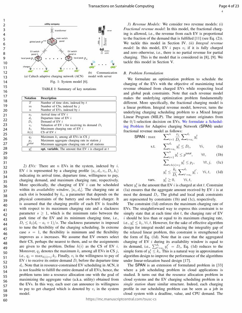
1) Charging Network: Our charging network model isinspired by the Caltech ACN [6] as illustrated in Fig. 1a. In theCaltech EV charging network (located in a parking garage),electricity is distributed through a two-level transformer archi-tecture from a main switch panel to multiple EV switch panels(2 panels in the current Caltech ACN). Each EV switch panelthen is connected to several chargers (≈25 chargers per panelin the Caltech ACN). The total power drawn from the mainswitch panel by the charging network has a power limit ofptotal, that is determined by the facility operator to control thecosts, reserve the capacity for other loads, and/or participate indemand-response programs. In other words, ptotal, which werefer to it as the global peak, hereafter, limits the maximumaggregate EV charging load at each time slot.

We assume that there are m EV switch panels that representm CSs. In addition to the global peak constraint, each CS jhas a capacity constraint on its total power drawn, indicatedby pj , and referred to it as the local peak constraint. Thevalue of pj is determined by the output power limit of thetransformers installed between the main switch panel and EVswitch panels and could be different for each EV switch panel.It is often observed that the charging demand of different CSs(EV switch panels in Fig. 1a) are well below the local peakconstraints. To increase the flexibility due to heterogeneouscharging demand of CSs, in the Caltech ACN, the global peakconstraint of the main switch can be over-provisioned, i.e.,ptotal is less than the aggregate local peaks, (

∑j pj ≥ ptotal).

While this increases flexibility, it also couples the problem ofEV charging scheduling across different CSs. Our solutionsin this paper will be centralized ones which can be obtainedthrough communication between the CSs and a central serveras illustrated in Fig. 1b.

Page 3 of 23



123456789101112131415161718192021222324252627282930313233343536373839404142434445464748495051525354555657585960

4

utility company

main switch panel

EV switch panel 1

charger

transformer

EV switch panel m

local peak1p local peak

mp

global peak totalp

(a) Caltech adaptive charging network (ACN)

server

access point

dat

a

com

man

d

(b) Communicationmodel with server

Fig. 1: System model [6].

TABLE I: Summary of key notations

Notation DescriptionT Number of time slots, indexed by tm Number of CSs, indexed by jn Number of EVs, indexed by iai Arrival time of EV idi Departure time of EV iDi Demand of EV ivi Valuation of EV i for receiving its demand Diki Maximum charging rate of EV ih(i) CS of EV i

qj Maximum ki among all EVs in CS jpj Maximum aggregate charging rate in station jptotal Maximum aggregate charging rate of all stationsyti opt. variable, The amount that EV i is charged at t

2) EVs: There are n EVs in the system, indexed by i.EV i is represented by a charging profile 〈ai, di, vi, Di, ki〉indicating its arrival time, departure time, willingness to pay,charging demand, and maximum charging rate, respectively.More specifically, the charging of EV i can be scheduledwithin its availability window, [ai, di]. The charging rate ateach slot is bounded by ki, a parameter that depends on thephysical constraints of the battery and on-board charger. Itis assumed that the charging profile of each EV is feasiblewith respect to its maximum charging rate and a slacknessparameter s ≥ 1, which is the minimum ratio between thepark time of the EV and its minimum charging time, i.e.,Di ≤ ki(di − ai + 1)/s. The slackness parameter is imposedto tune the flexibility of the charging scheduling. In extremecase s = 1, the flexibility is minimum and the flexibilityimproves as s increases. We assume that EV owners selecttheir CS, perhaps the nearest to them, and so the assignmentsare given to the problem. Define h(i) as the CS of EV i.Moreover, qj denotes the maximum ki among all EVs in CS j,i.e., qj = maxh(i)=j ki. Finally, vi is the willingness to pay ofEV i to receive its entire demand Di before the departure timedi. Note that in resource-constrained EV scheduling in ACN, itis not feasible to fulfill the entire demand of all EVs, hence, theproblem turns into a resource allocation one with the goal ofmaximizing the aggregate value (a.k.a. utility) obtained fromthe EVs. In this way, each user can announce its willingnessto pay to get charged which is denoted by vi in the systemmodel.

3) Revenue Models: We consider two revenue models: (i)Fractional revenue model: In this model, the fractional charg-ing is allowed, i.e., the revenue from each EV is proportionalto the fraction of the demand that is fulfilled [11] (see Eq. (2)).We tackle this model in Section IV. (ii) Integral revenuemodel: In this model, EV i pays vi if it is fully chargedand zero otherwise, i.e., there is no partial revenue for partialcharging. This is the model that is considered in [8], [9]. Wetackle this model in Section V.

B. Problem Formulation

We formulate an optimization problem to schedule thecharging of the EVs with the objective of maximizing totalrevenue obtained from charged EVs while respecting localand global peak constraints. Note that each revenue modelmakes the underlying optimization problem fundamentallydifferent. More specifically, the fractional charging model isa linear problem. Integral revenue model, however, turns theunderlying charging scheduling problem to a Mixed IntegerLinear Program (MILP). The integer nature originates fromthe 0/1-selection decision on EVs. We formulate a Schedul-ing Problem for Adaptive charging Network (SPAN) underfractional revenue model as follows:

SPAN : max∑n

i=1

viDi

∑di

t=ai

yti

s.t.∑di

t=ai

yti ≤ Di, ∀i, (1a)∑n

i=1yti ≤ ptotal, ∀t, (1b)∑

i:h(i)=jyti ≤ pj , ∀t, j, (1c)

yti ≤kiDi

∑di

t′=ai

yt′

i , ∀i, t, (1d)

vars. yti ≥ 0, ∀i, t,where yti is the amount that EV i is charged at slot t. Constraint(1a) ensures that the aggregate amount received by EV i is atmost the demand Di. The global and local peak constraintsare represented by constraints (1b) and (1c), respectively.

The constraint (1d) enforces the maximum charging rate ofEVs. The straightforward way to express this constraint is tosimply state that at each time slot t, the charging rate of EVi should be less than or equal to its maximum charging rate,i.e., yti ≤ ki,∀i, t. However, for the sake of effective algorithmdesign for integral model and reducing the integrality gap ofthe relaxed linear problem, this constraint is strengthened inthe form of Eq. (1d). Note that in case that the aggregatedcharging of EV i during its availability window is equal toits demand, i.e.,

∑di

t′=aiyt

′

i = Di, Eq. (1d) reduces to thesimple form of yti ≤ ki. This is a natural way in approximationalgorithm design to improve the performance of the algorithmsunder linear-relaxation based design [17].

The SPAN is an extension of formulated problem in [33]where a job scheduling problem in cloud applications isstudied. It turns out that the resource allocation problem incloud systems and the EV charging scheduling problem in asingle station share similar structure. Indeed, each chargingprofile in our scheduling problem can be seen as a job incloud system with a deadline, value, and CPU demand. The

Page 4 of 23



123456789101112131415161718192021222324252627282930313233343536373839404142434445464748495051525354555657585960

5

TABLE II: Proposed algorithms and their properties.

Algorithm Revenue model Type Optimality ComplexityFCS fractional offline Optimal O(n2T + nT 2)

ICS integral offline(

1 +∑mj=1

pjpj−qj

. ss−1

)-approximate O(nT log T + n2T )

FOCS fractional online 2-competitive O(n2T )IOCS integral online b(1 + p

p−q .ss−1

)-competitive, (m = 1) O(n2T )

SPAN, however, comes with an additional constraint (1b),which makes it different from the problem in [33], such thatthe existing solution will not work in the new setting. Moreimportantly, this paper studies both offline and online solutionsfor the problem in both fractional and integral settings, while[33] tackles only the offline integral model.

IV. FRACTIONAL REVENUE MODEL

In the fractional model, the revenue of the CS from EV iis directly proportional to the amount of resource that the EVis received, i.e.,

vfi =

∑t y

ti

Divi, (2)

where vi is the gain, if the entire demand Di is fulfilled andvfi is the fractional gain.

We propose a simple algorithm, called FCS, with lowcomputational complexity of O(n2T +nT 2) for the fractionalmodel that finds the optimal solution in offline setting. Notethat even though linear programs can be solved in polynomialtime in general, the complexity of our proposed algorithmis much lower than the general linear program algorithms.Moreover, our proposed offline algorithm applies a valley-filling strategy to reduce the peak. A summary of proposedalgorithms with their complexity and assumptions is given inTable II.

A. Optimal Offline Design

In this section, we propose an optimal algorithm for offlinefractional model. As a natural solution, one may think of agreedy algorithm as follows: at each time slot, charge theEV(s) with highest unit-value and process others if onlythe remaining resource cannot be allocated to the selectedEV(s) (e.g., due to maximum charging rate constraint orfulfillment of the EVs’ demand). This approach is a popular,yet straightforward method in the scheduling. However, it turnsout that this approach cannot provide an optimal solution tothe problem even in fractional revenue model. In fact, thissolution is only 2-approximation (i.e., the profit obtained bythe algorithm would be 1/2 of the optimum). As an intuitionof the proof think of two EVs in a single charging stationwith power capacity p and v1

D1− v2

D2= ε where ε > 0 is an

arbitrary small number, a1 = a2 = 1, d1 = 2, d2 = 1 andD1 = D2 = k1 = k2 = p. Then, applying the simple greedy,EV 1 will be selected at time slot 1 and EV 2 will have nochance to get charged due to its deadline constraint while EV1 could wait until time slot 2 and still receive all its demand.

We refer the proposed algorithm in this secion as theFCS and summarize it as Algorithm 1. The FCS works intwo phases. In the first phase (Section IV-A1), the algorithm

decides on the amount of resource to be allocated to eachEV within its availability window and reserves resourcesaccordingly. In this phase, the details of allocation is notknown. The actual resource allocation is done in the secondphase (Section IV-A2) by setting variables yti .

Before discussing the details of the algorithm, we givea definition and introduce some notations to facilitate ouralgorithm design.

Definition 1. Time interval [δ, δ′] is a “super interval” forinterval [t, t′] if 1 ≤ δ ≤ t AND t′ ≤ δ′ ≤ T . Moreover,It,t′ is the set of all super intervals of interval It,t′ i.e.,It,t′ = {[δ, δ′] : 1 ≤ δ ≤ t AND t′ ≤ δ′ ≤ T}.

The number of super intervals of an interval is at most T 2

and at least one (for interval [1, T ]).Let Ri be the amount of resource that is reserved for EV

i by the FCS and It,t′ as time interval [t, t′]. Then, assumingthat charging demands are sorted in non-increasing order oftheir unit values, Ai

j(t, t′) is the aggregate residual resource

in interval It,t′ at station j assuming that the reservation forEVs 1 to i is accomplished. We now explain in detail eachphase of the algorithm.

1) Phase I-Reservation: In Line 1, the EVs are sorted in anon-increasing order of their unit values. In Line 5, the FCSprocesses demand of EV i, picked from top of the ordered list,and sets Ri as the amount to be reserved for EV i which willbe allocated in Phase II. In Line 7, the residual resource of allintervals in set Iai,di

decreases by Ri and EV i is added tothe set of selected EVs.

Lemma 1. Provided that for EV i we have

Ri ≤ min

{Di,min

t,t′Ai−1

j (t, t′),∀t, t′ : It,t′ ∈ Iai,di

}(3)

with a dummy A0j (t, t′) defined as A0

j (t, t′) = (t′ − t + 1) ×min{ptotal, pj}, then there is a feasible allocation to allocateRi to EV i in its availability window [ai, di].

In Lemma 1, A0j (t, t′) indicates the available resource when

no charging request is processed in It,t′ . In Eq. (3), thesecond term, i.e., mint,t′ A

i−1j (t, t′), indicates the minimum

remaining resource in all super intervals of interval Iai,di. For

i ≥ 1, Aij(ai, di) is defined as follows:

Aij(ai, di) =

{Ai−1

j (ai, di)−Ri j = h(i),

Ai−1j (ai, di) j 6= h(i).

The optimal value of Ri, i = 1, . . . , n is set according tothe following lemma:

Lemma 2. Given n EVs sorted in a non-increasing orderof the unit values, v1/D1 ≥ v2/D2 ≥ · · · ≥ vn/Dn, and the

Page 5 of 23



123456789101112131415161718192021222324252627282930313233343536373839404142434445464748495051525354555657585960

6

Algorithm 1: FCSInput: n EVs with their profile, local and global peak

constraints pj , j = 1, . . . ,m and ptotal

Output: Optimal scheduling under fractional model

1 Sort charging requests in non-increasing order of theirunit values, i.e., v1

D1≥ v2

D2≥ · · · ≥ vn

Dn

2 L ← ∅3 //Phase I4 for i = 1, . . . , n do5 Ri ← min{Di,min

t,t′Ai−1

h(i)(t, t′), ∀t, t′ : It,t′ ∈

Iai,di}6 if Ri > 0 then7 Ai

h(i)(t, t′)← Ai−1

h(i)(t, t′)−Ri,∀t, t′ : [t, t′] ∈

Iai,di

8 L ← L ∪ i

9 //Phase II10 Sort EVs in L in increasing order of their charging

flexibility i.e., (di−ai+1)ki

Di, i ∈ L.

11 for i = 1, . . . , |L| do12 Pick EV i from the sorted list L.13 feasible←

(∑di

t=aimin{ki, Ai−1

h(i)(t, t)})−Ri

14 if feasible < 0 then15 Re-allocate previously allocated EVs such that

feasible ≥ 0

16 Arbitrarily allocate Ri to EV i in its availabilitywindow

value of Ri, where Ri is set after Ri−1, i = 2, . . . , n byEq. (3), then,

Ri = min

{Di,min

t,t′Ai−1

h(i)(t, t′),∀t, t′ : It,t′ ∈ Iai,di

},∀i,

is the optimal value for Ri.

2) Phase II- Allocation: Lemma 1 shows that there is afeasible scheduling to allocate the reserved resources. How-ever, despite its feasibility, it is not straightforward to findsuch a schedule. For example, assume that for EV i, Ri = 10and ki = 4. It is possible that all available resources areconcentrated in a single time slot but EV i cannot usemore than 4 kWh of it. In this situation, the previouslyallocated resources in interval Iai,di

should be re-allocatedsuch that the concentrated resources are dispersed and wehave

∑di

t=aiσt ≥ Ri where σt = min{ki, Ai−1

h(i)(t, t)} is themaximum resource that can be allocated to EV i at time slot t.Since the total amount of allocated resource does not changein the interval, such dispersion is possible and can be doneby a simple algorithm in which allocates min{ki, Ai−1

h(i)(t, t)}starting from time slot t = ai until Ri units is allocated.To further reduce the peak of the system, we will developSMARTALLOCATE algorithm (See Section V) which acts moreintelligent so that Line 16 of the FCS can be replaced by “RunSMARTALLOCATE(i, Ri)”.

Theorem 1. FCS is an optimal solution under fractionalrevenue model.

The following theorem characterizes the complexity of FCS.

Theorem 2. The time complexity of FCS algorithm isO(n2T+nT 2) where n is the number of EVs and T is numberof time slots.

B. Online Scenario

In this section, we devise an algorithm for the scenario thatEVs arrive in online fashion. The scheduling decisions at eachtime slot are made given the information of available EVs andneither exact values nor stochastic modeling of future arrivalsis available. Our goal is to obtain a competitive ratio for theonline algorithm. A scheduling algorithm A is c-competitivefor c ≥ 1 if the revenue obtained by the optimal offlinealgorithm is at most c times the algorithm A’s revenue forany input sequence [15].

The proposed online algorithm for the fractional model,referred to as FOCS, is listed as Algorithm 2. The FOCS isa simple yet efficient algorithm that always selects EVs withhighest unit value to allocate as follows. First, the algorithmsorts the available EVs at each time slot t based on their unitvalue (Line 2). In this step, the algorithm breaks ties basedon EVs’ deadline i.e., if two EVs have the same unit value,then the one with earliest deadline comes first in the sortedlist. Next, the FOCS selects one EV at a time from the sortedlist to allocate with maximum charging rate considering theEV’s remaining demand, maximum charging rate, and peakconstraints (Lines 3-4). The allocation is continued until allresources are allocated or there is no more EV that couldbe allocated. The time complexity of the FOCS is O(n2T ),determined by cost of its “for” loop multiplied by total numberof times that the algorithm needs to be run.

Algorithm 2: FOCS: ∀t ∈ {1, 2, . . . , T}

1 Mt ← The set of available EVs that not received their entiredemand by t

2 Sort EVs in set Mt indexed by i = 1, . . . , |Mt|:v1/D1 ≥ v2/D2 ≥ · · · ≥ v|Mt|/D|Mt|, where ties are brokenbased on users’ deadline (giving priority to the users with earliestdeadline)

3 for i = 1, . . . , |Mt| do4 yti ← min{ki, Di −

∑tτ=ai

yτi , ph(i) −∑i′:h(i′)=h(i) y

ti′ , p

total −∑i′ y

ti′}

Despite the simplicity of FOCS which makes it easy toimplement, its performance is sound and within a constantfactor of the offline optimum. We now proceed to analyze theperformance of the FOCS by first giving some preliminaries.

Fix an optimal scheduling and let SFOCS,t and SOPT,t be thesets of EVs selected by the FOCS and optimal solution at timeslot t, respectively. Let yti and zti be the charging rate of EV iset by FOCS and OPT, respectively. We define ∆t

i as follows:

∆ti =

{min{zti − yti , ri,t} i ∈ SOPT,t, z

ti > yti ,

0 otherwise,(4)

where ri,t is the remaining demand of EV i by the end of timeslot t. ∆t

i > 0 indicates that the optimal algorithm allocated∆t

i units more resources to EV i than the FOCS by time slot

Page 6 of 23



123456789101112131415161718192021222324252627282930313233343536373839404142434445464748495051525354555657585960

7

t that could be feasibly allocated by FOCS to the EV i. If forany EV i ∈ SOPT,t and time slot t ∈ T we have yti = zti ,i.e., ∆t

i = 0, then the FOCS is obviously optimal because itgains whatever the optimal solution gains. We define loss ofthe FOCS imposed by EV i as follows:

li,t = ∆ti

viDi, (5)

Note that the loss always takes a non-negative value as∆t

i ≥ 0. When FOCS sets charging rate of an EV less thanits rate in the optimal solution, it gains ∆t

ivi/Di less than theoptimal solution from that EV. An upper bound for the distancebetween the optimal objective value (denote by OPT) and therevenue of the FOCS (denote by ALG) is summation of thelosses over all time slots and all EVs, i.e.,

OPT − ALG ≤T∑

t=1

∑i∈SOPT,t

li,t. (6)

In addition to the amount of loss, the gain of the algorithmfrom charging alternative EVs should also be taken intoaccount in comparison between OPT and ALG.

Let i ∈ SOPT,t, i /∈ SALG,t and gi,t be the gain that theFOCS obtains from charging another EV instead of i at timeslot t. We are going to show that in the FOCS, for each EVi with li,t > 0 there must be another EV (denote by i′)where yti′ ≥ ∆t

i and vi′Di′≥ vi

Diwhich means in resource

allocation phase for EV i, the FOCS allocated the difference∆t

i to another EV with the same or higher unit value. Thiscan be proved by considering the fact that (i) the selectedEVs have higher unit values than the unselected EVs, and (ii)the charging rate of the selected EVs are set to the maximumfeasible value. Moreover, the FOCS is “work-conserving” i.e.,it does not let any resource remain unused if there are someEVs that can use it.

Let gi,t denote the gain that FOCS obtains from allocatingthe same amount of resource that optimal algorithm allocatedto EV i (with size zti ) to another EV(s). If ∆t

i = 0, the lossis zero. If ∆t

i > 0, then by the charging strategy that theFOCS uses we can conclude that (i) i is not finished by theFOCS, and (ii) no more resources from station ph(i) can befeasibly allocated, otherwise, the FOCS could allocate moreresources to EV i. Therefore, the ∆t

i units of the resource areallocated to one or multiple other EVs (denote them by setJ ti ) by the FOCS. Moreover, it must hold that all the EVs in

set J ti have a unit value equal to or higher than vi/Di which

yields gi,t ≥ li,t, otherwise, the FOCS should not prefer theEVs in J t

i to i. Since the result holds for any arbitrarily EVi, we can get the following:

n∑i=1

T∑t=1

li,t ≤n∑

i=1

T∑t=1

gi,t. (7)

Moreover, the total gain of FOCS, i.e., ALG, is equal tosum of its gains from each single EV:

ALG =n∑

i=1

T∑t=1

gi,t. (8)

With the above discussion and using Eqs. (6), (7) and (8)we are able to derive a competitive ratio of 2 for the FOCS.

Theorem 3. The FOCS is 2-competitive.

Remarks: When there is only one CS and EVs have no limiton their charging rate, the FOCS is identical to the FIRSTFITalgorithm [34] which is known to be 2-competitive for classicjob scheduling problem. However, the charging rate limitationis crucial for EV charging problem. Moreover, [34] uses a“charging argument” to prove the competitive ratio of theproposed algorithm which cannot be directly applied to ourproblem. Thus, the FOCS extends the FIRSTFIT and makesit practical for the EV charging scenario. Moreover, the prooftechnique used for the competitive analysis of the FOCS isfundamentally different from the one used in [34].

V. INTEGRAL REVENUE MODEL

The MILP form of the SPAN in integral model is a general-ized form of the 0/1-knapsack problem which is a well-knownNP-hard problem. To give an intuition, consider the schedulingproblem in a single time slot (i.e, T = 1). Then, allocatingpower resources to the EVs is equivalent to allocating thecapacity of knapsack to the items. In Section V-A, we proposea fast polynomial time offline approximation algorithm for theintegral problem. In Section V-B, we extend the result andpropose an online algorithm for the integral model.

A. Offline Scenario

We design our offline scheduling algorithm under integralmodel referred to as ICS, to solve the SPAN approximately.Since the performance analysis of the proposed algorithm re-lies on a dual fitting method and utilizes weak duality property,we first need to construct the dual problem of SPAN. Towardthis, we introduce variables α, β, γ and π. Generally, in primal-dual approximation algorithm design, each constraint (resp.variable) in primal (resp. dual) problem is associated with avariable (resp. constraint) in dual (resp. primal) problem. Inour case, constraints (1a) (1b), (1c) and (1d) in the SPANare respectively associated with dual variables α, β, γ and π(for more details see [16]). The dual problem is formulated asfollows:

minn∑

i=1

Diαi +m∑j=1

T∑t=1

pjβ(t) +T∑

t=1

ptotalγ(t)

s.t. αi + β(t) + γi + π(t)− kiDi

di∑t′=ai

πi(t′) ≥ vi

Di,

∀i, t ∈ [ai, di], (9a)vars. αi, βi, γ, πi(t) ≥ 0, ∀i, t.1) Explanation of the Main Algorithm: Our algorithm de-

sign is inspired by the basic algorithm proposed in [33]. Thealgorithm in [33], however, works for a single CS where arrivaltime of all EVs are the same and there is no global peakconstraint. The ICS algorithm (listed as Algorithm 3) worksin two phases. In the first phase it sorts the charging requestsbased on their unit values in a non-increasing order. Then,it selects most valuable demand. If the remaining resource isenough to cover the entire demand of the EV, it is admittedto receive the demand (Lines 6-7).

Scheduling of the Selected EV: If the feasibility checkpassed (Line 6 in Algorithm 3), ICS calls sub-procedure

Page 7 of 23



123456789101112131415161718192021222324252627282930313233343536373839404142434445464748495051525354555657585960

8

SMARTALLOCATE to allocate required resources in interval[ai, di]. Then, αi is set to vi/Di in order to cover dualconstraint in Eq. (9a) (Lines 7-8).

In SMARTALLOCATE, let us define W (t, h(i)) =∑i′:h(i′)=h(i) y

ti′ as total workload at time slot t in

CS h(i) and W (t, h(i)) as total available load toallocate at time slot t for CS h(i). We always haveW (t, h(i)) +W (t, h(i)) = ph(i),∀t, i. For scheduling,SMARTALLOCATE applies two main policies: 1) valley-fillingand, 2) right-to-left allocation. With valley-filling, the slotswith more available resources are preferred which helpsto reduce the peak of the system. Right-to-left allocationis used when two or more time slots are equal in termsof their remaining resources. A ranking based approach isused to apply the aforementioned policies. To charge EV i,SMARTALLOCATE ranks time slots in interval [ai, di]. Then,charging is done by allocating resources from the higherranked time slot to lowest one. The rank of a time slot tis calculated based on remaining resources in the time slot(valley-filling) and value of t (right-to-left allocation).

Algorithm 3: ICS

1 initialize: y ← 0, α← 0, β ← 0, γ ← 0, π ← 02 Sort charging requests in non-decreasing order of their unit values:

v1/D1 ≥ v2/D2 ≥ · · · ≥ vn/Dn3 for (i=1. . . n) do4 for t = ai . . . di do5 σt ← min

{ph(i) −

∑i′:h(i′)=h(i) yi′ (t),

ptotal −∑ni′=1 y

ti′ , ki

}6 if Di ≤

∑dit=ai

σt then7 SMARTALLOCATE(i,Di)8 αi ← vi/Di

9 else10 if (β(di) = 0) then11 BETACOVER(i)

12 for (i=1. . . n) do13 if EV i is not selected then14 RECONSIDER(i);

Dual Feasibility of the Non-selected EVs: If remainingpower resource is not enough to fully charge EV i, i.e.,Di >

∑di

t=aiσt, the EV cannot be selected. However, we

still need to satisfy constraint (9a) in dual problem which isdone by calling BETACOVER(i). To cover the constraint (9a)for EV i, sum of dual variables for all t ∈ [ai, di] shouldbe greater than or equal to vi/Di. BETACOVER(i) sets β(t)to vi/Di for all time slots t in interval [tcov, R(di)] (Lines3-4 of Algorithm 5). Observe that β(t′) ≥ vi/Di,∀t′ < tcov(with tcov > 1) considering that the demands are sorted ina non-increasing order of the unit-values and β(t′) is alreadyset to vi′/Di′ when processing the earlier charging demand ofEV i′ which is not selected. Hence, vi′/Di′ ≥ vi/Di, therebyβ(t) ≥ vi/Di, and the dual constraint in (9a) is satisfied. Lines1-4 of BETACOVER is enough to cover the dual constraint.However, the algorithm continues in Lines 5-8 by setting avariable Φi′(t) for time slots t = 1, . . . , R(di) to a valuedependent to amount of the resource that a selected EV i′

received at slot t. Φi′(t) will be used in approximation analysisof the main algorithm and has no effect on the scheduling ofEVs.

Algorithm 4: SMARTALLOCATE(i,Di)Input: EV i to receive Di from CS h(i)

1 Rank time slots in interval [ai, di] such that for any t1 and t2:rank(t1) > rank(t2) iff W (t1, h(i)) > W (t2, h(i)) ORW (t1, h(i)) == W (t2, h(i)) ∧ t1 > t2

2 while∑dit′=ai

yt′i 6= Di do

3 Select time slot t with highest rank which is not selected before4 Allocate

min{ki, W (t, h(i)), Di −

∑tτ=ai

yτi , ptotal −

∑i′ y

ti′

}to

EV i at t

Algorithm 5: BETACOVER(i)

1 tcov ← min{t : β(t) = 0}2 R(di) = max{t ≥ di : ∀t′ ∈ (di, t], W (t′) < qh(i)}3 for (t = tcov . . . R(di)) do4 β(t)← vi/Di

5 for (t = 1 . . . R(di)) do6 for (i′ = 1 . . . n)) do7 if yt

i′ > 0 ∧ Φi′ (t) = 0 then8 Φi′ (t)←

[ ph(i)

ph(i)−kiss−1

]. viDiyti′

Algorithm 6: RECONSIDER(i)1 L ← ∅2 vinc ← vi3 σt ← 0, t = ai, . . . , di4 for (i′ = i− 1 . . . 1) do5 if EV i′ is selected ∧(h(i′) = h(i)) ∧ (vinc − vi′ ) > 0 then6 Add EV i′ to list L7 vinc ← vinc − vi′8 for (t = ai . . . di) do9 σt ← σt + min{ki, yti′}

10 if∑dit=ai

σt ≥ Di then11 Remove EVs in list L from charging schedule12 SMARTALLOCATE(i,Di)

Improving the Gain: In the second phase, the ICS tries to in-crease total value of selected EVs by calling RECONSIDER(i)on every unselected EV i (Lines 12-14). The RECONSIDER(i)(listed as Algorithm 6) checks that whether the total revenuecan be increased by replacing some selected EVs with EV ior not (Lines 4-9). If such EVs are found, the algorithm stopstheir charging and allocates EV i using SMARTALLOCATE(Lines 10− 12).

2) Analysis: In a primal-dual algorithm, the goal is todesign an algorithm in a way that it produces a good solutionfor primal problem (with primal value Γ) and a feasiblesolution for the dual problem (with dual value Λ). Then,assuming that the primal problem is a maximization problem,to prove that the algorithm is c−approximation (for c ≥ 1),the important part is to show that Λ ≤ cΓ. Then, based onweak duality theorem we have Λ ≥ OPT, and it is concludedthat Γ ≥ 1

c × OPT where OPT is the optimal value. Based

Page 8 of 23



123456789101112131415161718192021222324252627282930313233343536373839404142434445464748495051525354555657585960

9

on the above understanding, the following theorem scrutinizesthe approximation ratio of the ICS assuming that arrival timesare the same for all EVs.

Theorem 4. ICS algorithm is a(

1 +∑m

j=1pj

pj−qj .s

s−1

)-

approximation when EVs have same arrival time.

Note that in the case that the system is flexible enough, i.e.,s� 1, and the maximum charging rates of stations are muchbigger than those of EVs, i.e., pj � qj ,∀j, the approximationratio approaches m+1. And in the case that there is one singlestation, the approximation ratio is 2.

B. Online ScenarioDue to the binary selection variable, the online solution

design under integral model is more challenging than the onefor fractional model. We propose IOCS that is built upon theoffline ICS. In particular, the IOCS calls the ICS at each timeslot for the set of available EVs, however, any algorithm thatis designed for offline integral model can be used alternatively.Hereinafter, A refers to the ICS or a similar algorithm.

Algorithm 7: IOCS: ∀t ∈ {1, 2, . . . , T}

1 Let A be an algorithm that solves the problem with a1 = · · · = an2 Rt ← set of EVs arrived at time slot t3 Mt ←Rt ∪ {i : t ∈ Ti AND

∑t′ y

t′i < Di}

4 Based on the residual in interval [t, T ], use algorithm A to allocateEVs in set Rt assuming no further arrivals

5 SIOCS,t ← {i : i ∈Mt AND i is admitted at t}6 ΓA,Rt ←

∑i∈SIOCS,t

vi7 Assume all reserved resources are freed at time slots t, t+ 1, . . . , T8 ri,t ← remaining demand of i at t, ∀i9 D′i ← ri,t, v′i ←

ri,tDi

vi, ∀i ∈Mt

10 Run A on Mt using D′i and v′i, ∀i and reconstruct SIOCS,t11 ΓA,Mt ←

∑i∈SIOCS,t

vi \\Use original values

12 if ΓA,Mt > ΓA,Rt then13 Use the second schedule

14 else15 Use the first schedule

The IOCS is summarized as Algorithm 7. At slot t, the IOCScompares two scheduling results returned by A and choosesamong them. In the first scheduling, the IOCS keeps all re-served resources in interval [t, T ] intact. Then, for utilizing theremaining resources, the algorithm runs A over arrived EVs attime slot t. In this case, the total revenue obtained by the activeEVs (i.e., EVs that are available but not received their entiredemand yet) is denoted by ΓA,Rt (Line 6 of the algorithm).In the second scheduling, the IOCS considers the case thatit can sacrifice the previously admitted EVs by cancelingtheir reservations and allocating the freed resources to morevaluable demands. For this purpose, the algorithm modifiesthe demand and valuation of the previously admitted EVs suchthat each demand is replaced by the EV’s remaining demand,and the valuation of the EV is proportionally calculated basedon the remaining demand (Line 9 of the algorithm) so thatthe unit values of EVs do not change. Then, the IOCS runsA on set of active EVs Mt where the corresponding gain isdenoted by ΓA,Mt . If ΓA,Mt > ΓA,Rt , the IOCS forgets thepreviously admitted EVs and follows the second scheduling.

TABLE III: EV models and their battery capacity.

Model Battery Model BatteryMitsubishi i-MiEV 16 kWh Citroen C-Zero 14 kWhPeugeot iOn 16 kWh Honda Clarity 25.5 kWhHyundai Kona 64 kWh Nissan LEAF 40 kWhHyundai Ioniq 28 kWh BMW i3 22/33 kWhTesla Model S/X 60/100 kWh Kia Soul EV 27 kWh

The following theorem characterizes the competitive ratioof the IOCS in a special case.

Theorem 5. Let A be ICS in IOCS algorithm and m = 1.Assuming that EVs are released in b distinct groups wherearrival time of EVs in each group are the same, the IOCSis b(

1 + pp−q

ss−1

)-competitive with optimal offline solution,

where p is the station peak and q = maxi ki, i = 1, . . . , n.

VI. SIMULATION RESULTS

Simulation Setup and Overview: We consider chargingscheduling of EVs during a period of 12 time slots of length 1hour (e.g., from 08:00 to 20:00). We gathered information of12 popular EV models in the market to use in the simulation.Each EV model is characterized by its battery capacity asshown in Table III and maximum charging rate. Tesla modelscan get charged with up to 100 kW using Tesla super chargers.Also, all other models have rapid DC charging capability (upto 50 kW) with CHAdeMO method. This setting for chargingrates is in accordance with future DCFC systems that can haveseveral fast DC chargers installed in the charging station. Thepeak intervals include 08:00-10:00, 12:00-14:00, and 18:00-20:00 according to NHTS survey [4], [35]. The probabilityof an EV’s arrival during the peak hours is two times higherthan the off-peak periods. Demands are uniform random valuesfrom [ 12Ui, Ui] where Ui is the battery capacity for EV i inTable III. The deadline of each EV is set according to slacknessparameter s (with default value of 1.2), its demand andmaximum charging rate of the battery as di = ai + dDis

kie−1.

EVs are assigned to different CSs randomly and given asinput to the algorithms. The willingness to pay by each userfor one kWh of power is a random uniform number frominterval [ 12z,

32z] where z = $0.11 is national average price

of electricity in the US [36]. In the simulation, the results areplotted with 95% confidence level and each point representsaverage result of 50 random scenarios. Table IV explains thecomparison algorithms including current implemented algo-rithm in Caltech ACN referred to as IOLP [6] and its adaptedversion for the fractional revenue model FOLP. The IOLP andFOLP algorithms runs as follows: at each time slot assume thatthere will be no further arrivals and solve the optimizationproblem (e.g., by commercial solvers) for the current set ofEVs and their remaining demands. In Table IV, the letters “I”,“F” and “O” in front of the algorithms’ name refer to integral,fractional and online types, respectively.

The measured performance metrics are total revenue, per-centage of EVs that received all their demand, and total peak.To calculate optimal solution in integral revenue model, weused Gurobi solver [37].

Evaluation Based on Total Revenue: Fig. 2 depicts thecomparison results based on total revenue under fractional and

Page 9 of 23



123456789101112131415161718192021222324252627282930313233343536373839404142434445464748495051525354555657585960

10

100 150 200 250# of EVs

100

150

200

250

Tot

al r

even

ue

fCS foCS iOPT iCS ioCS ioLP foLP

(a) m = 2

100 150 200 250# of EVs

200

250

300

350

400

Tot

al r

even

ue


(b) m = 4

100 150 200 250# of EVs

200

250

300

350

400

450

Tot

al r

even

ue


(c) m = 8

Fig. 2: Comparison results for 2, 4, and 8 CSs for fractional and integral revenue models. In the algorithms’ name, letters “o”, “f” and “i”indicate online, fractional and integral, respectively. Note that a “non-optimal” fractional algorithm can potentially achieve better result thanan “optimal” integral algorithm due to higher flexibility in power allocation.

200 300 400 500 600Local peak constraint

300

350

400

450

500

550

Tot

al r

even

ue

GreedyRTLiCSioCS

(a) Total revenue


200

300

400

500

600

Act

ual p

eak

GreedyRTLiCSioCS

(b) Actual global peak


50

60

70

80

90

100

% o

f ful

ly c

harg

ed E

Vs

GreedyRTLiCSioCS

(c) % of full charged EVs

Fig. 3: Comparison in terms of total revenue, actual peak, and percentage of fully charged EVs by varying local peak value.

TABLE IV: Acronyms for the algorithms

Notation DescriptionIOPT Optimal value under integral revenue modelICS Proposed offline algorithm for SPAN under integral

revenue modelFCS Proposed optimal algorithm for SPAN under frac-

tional revenue modelIOCS Proposed online algorithm for SPAN under integral

revenue modelFOCS Proposed online algorithm for SPAN under frac-

tional revenue modelIOLP Algorithm in [6] (works under integral revenue

model)FOLP Adaptation of algorithm in [6] for fractional revenue

modelGreedyRTL The algorithm in [33] for single station scenario

without global peak constraint (works under integralrevenue model)

integral models while the total number of EVs increases from100 to 250 for 2, 4, and 8 CSs. The local and global peakconstraints are set to 50 kWh and 200 kWh, respectively.

The proposed algorithms are compared to the optimaloffline solution of integral model (IOPT) and IOLP. Notethat comparison with offline optimal could be considered as abaseline comparison with the category of approximate offlinealgorithms in integral model [39].

Recall that FCS is optimal offline solution. The notableobservations are as follows: (i) the general trend in scenario ofFig. 2 is that by increasing the number of EVs, total revenueincreases. This is because with more number of EVs, thescheduler has more freedom to choose more valuable EVs. (ii)as explained in Section IV, under fractional charging model,better results are expected due to increased scheduling flexibil-ity in CSs. According to the simulation data that we extracted

from Fig. 2, the gain obtained by FCS and FOCS in Fig. 2 arerespectively 12% and 10% more than the gain of the ICS andIOCS. (iii) In Fig. 2a and Fig. 2b, sum of the local peaks isless than or equal to the global peak while in Fig. 2c this sumis two times greater than the global peak. Consequently, thetotal revenue significantly improved when the number of CSsis increased from 2 to 4 while there is a slight improvementfrom 4 to 8 CSs as the global peak constraint prevents thealgorithms from charging more EVs. (iv) in integral revenuemodel, the proposed IOCS algorithm acts significantly betterthan IOLP. In particular, IOCS improves IOLP by 38%, 36%,and 32% for m = 2, m = 4 and m = 8, respectively.In fractional revenue model, however, there is a very slightdifference between FOCS and FOLP. (v) ICS approximatesIOPT by 97%, 94%, and 95% for m = 2, m = 4, andm = 8, respectively. On average, IOCS is 90% of IOPT and,FOCS is 94% of its optimal offline solution, FCS. (vi) finally,the results depict that ICS achieves much better results inpractice as compared to the theoretical approximation ratiothat characterizes the performance in worst-case scenario.

Comparison Based on Actual Peak: The constraint set in theSPAN assures that any feasible solution respects the local andglobal peak constraints. An efficient scheduling algorithm maytake a further step by not only satisfying the peak constraintsbut to further reduce the peak as much as possible. Theproposed offline algorithms (i.e., ICS and FCS) apply valley-filling policy to reduce the peak. The online algorithms (i.e.,IOCS and FOCS) do not apply the same policy as they donot have future knowledge to be able to balance allocatedresources. To investigate the effect of employed valley-fillingstrategy, we conducted a set of simulations by varying localpeak constraints. The results of ICS is compared to IOCS

Page 10 of 23



123456789101112131415161718192021222324252627282930313233343536373839404142434445464748495051525354555657585960

11

and GreedyRTL [33] where the latter is an approximationscheduling for single station scenario with EVs having samearrival time (see the explanations after formulating the SPANin Section III-B). The results are shown in Fig. 3. Along withtotal revenue in Fig. 3a, we also report total actual peak inFig. 3b and percentage of fully charged EVs in Fig. 3c. In Fig.3a, the results for ICS and GreedyRTL are almost identicalwhile IOCS is 90% of the other two algorithms, on average.When pj ≥ 400, the total revenue for ICS and GreedyRTLdoes not increase in Fig. 3a and percentage of fully chargedEVs is 100 for both algorithms according to Fig. 3c. Fromthis point and onward, the scheduling is not challenging foroffline methods to obtain optimal answer because of resourcesufficiency. However, it is still a challenge to control totalactual peak for the system. As a result of valley-filling policy,the value of actual peak of ICS in Fig. 3b remains almostunchanged for pj ≥ 400. IOCS and GreedyRTL, however,continuously increase the peak demand, since they are notusing any peak shaving approach.

VII. CONCLUSION

This paper proposed offline and online algorithms for theEV charging scheduling problem under fractional and integralrevenue models in an adaptive charging network (ACN). Theproblem is different, and more challenging than the exist-ing single station EV charging scheduling problems since itrequires respecting the aggregate peak charging demand ofthe ACN. As the notable contributions, our proposed onlinealgorithm for fractional revenue model achieves constant com-petitive ratio of 2. Moreover, the offline integral algorithmachieves a theoretical bound on the optimality gap and ap-proximates the optimum by 92%, on average in experiments.As a future work, we plan to study the problem under postedpricing mechanism where the charging station publishes theunit price of the power (which can be varied over time) andthe users can accept or reject the offer. Another interestingfuture direction is to tackle the EV charging scheduling inmarket-based scenarios where the prices change over time.

REFERENCES

[1] “https://www.bloomberg.com/news/articles/2017-07-06/electric-cars-are-about-to-boost-global-power-demand-300-fold,” 2017.

[2] S. Zhao, X. Lin, and M. Chen, “Peak-minimizing online ev charging:Price-of-uncertainty and algorithm robustification,” in Proc. of IEEEINFOCOM, 2015.

[3] J. C. Mukherjee and A. Gupta, “A review of charge scheduling of electricvehicles in smart grid,” IEEE Systems Journal, vol. 9, no. 4, pp. 1541–1553, 2015.

[4] W. Tang, S. Bi, and Y. J. A. Zhang, “Online coordinated chargingdecision algorithm for electric vehicles without future information,”IEEE Transactions on Smart Grid, vol. 5, no. 6, pp. 2810–2824, 2014.

[5] D. Wu, H. Zeng, C. Lu, and B. Boulet, “Two-stage energy managementfor office buildings with workplace ev charging and renewable energy,”IEEE Transactions on Transportation Electrification, vol. 3, no. 1,pp. 225–237, 2017.

[6] G. Lee, T. Lee, Z. Low, S. H. Low, and C. Ortega, “Adaptive chargingnetwork for electric vehicles,” in Proc. of IEEE GlobalSIP, 2016.

[7] C.-K. Wen, J.-C. Chen, J.-H. Teng, and P. Ting, “Decentralized plug-inelectric vehicle charging selection algorithm in power systems,” IEEETransactions on Smart Grid, vol. 3, no. 4, pp. 1779–1789, 2012.

[8] Z. Zheng and N. Shroff, “Online welfare maximization for electricvehicle charging with electricity cost,” in Proc. of ACM e-energy,pp. 253–263, ACM, 2014.

[9] W. Tang and Y. J. A. Zhang, “A model predictive control approachfor low-complexity electric vehicle charging scheduling: optimality andscalability,” IEEE Transactions on Power Systems, vol. 32, no. 2,pp. 1050–1063, 2017.

[10] S. Chen and L. Tong, “iEMS for large scale charging of electric vehicles:Architecture and optimal online scheduling,” in Proc. of SmartGrid-Comm, 2012.

[11] Q. Xiang, F. Kong, X. Liu, X. Chen, L. Kong, and L. Rao, “Auc2charge:An online auction framework for eectric vehicle park-and-charge,” inProc. of ACM e-energy, pp. 151–160, ACM, 2015.

[12] V. Robu, E. H. Gerding, S. Stein, D. C. Parkes, A. Rogers, andN. R. Jennings, “An online mechanism for multi-unit demand andits application to plug-in hybrid electric vehicle charging,” Journal ofArtificial Intelligence Research, vol. 48, pp. 175–230, 2013.

[13] “http://www.pge.com/nots/rates/tariffs/rateinfo.shtml,” 2018.[14] Y. Zhang, M. Hajiesmaili, S. Cai, M. Chen, and Q. Zhu, “Peak-aware

online economic dispatching for microgrids,” IEEE Transactions onSmart Grid, vol. 9, no. 1, pp. 323–335, 2018.

[15] A. Borodin and R. El-Yaniv, Online computation and competitiveanalysis. cambridge university press, 2005.

[16] V. V. Vazirani, Approximation algorithms. Springer Science & BusinessMedia, 2013.

[17] R. D. Carr, L. K. Fleischer, V. J. Leung, and C. A. Phillips, “Strength-ening integrality gaps for capacitated network design and coveringproblems,” tech. rep., Sandia National Labs., Albuquerque, NM (US);Sandia National Labs., Livermore, CA (US), 1999.

[18] J. C. Mukherjee and A. Gupta, “Distributed charge scheduling ofplug-in electric vehicles using inter-aggregator collaboration,” IEEETransactions on Smart Grid, vol. 8, no. 1, pp. 331–341, 2017.

[19] P. M. de Quevedo, G. Munoz-Delgado, and J. Contreras, “Impact ofelectric vehicles on the expansion planning of distribution systemsconsidering renewable energy, storage and charging stations,” IEEETransactions on Smart Grid, 2017.

[20] M. Shafie-Khah, P. Siano, D. Z. Fitiwi, N. Mahmoudi, and J. P. Catalao,“An innovative two-level model for electric vehicle parking lots indistribution systems with renewable energy,” IEEE Transactions onSmart Grid, vol. 9, no. 2, pp. 1506–1520, 2018.

[21] Y. He, B. Venkatesh, and L. Guan, “Optimal scheduling for chargingand discharging of electric vehicles,” IEEE transactions on smart grid,vol. 3, no. 3, pp. 1095–1105, 2012.

[22] A. Malhotra, G. Binetti, A. Davoudi, and I. D. Schizas, “Distributedpower profile tracking for heterogeneous charging of electric vehicles,”IEEE Transactions on Smart Grid, vol. 8, no. 5, pp. 2090–2099, 2017.

[23] M. Moradijoz, M. P. Moghaddam, M. Haghifam, and E. Alishahi,“A multi-objective optimization problem for allocating parking lots ina distribution network,” International Journal of Electrical Power &Energy Systems, vol. 46, pp. 115–122, 2013.

[24] D. Wang, X. Guan, J. Wu, P. Li, P. Zan, and H. Xu, “Integrated energyexchange scheduling for multimicrogrid system with electric vehicles,”IEEE Transactions on Smart Grid, vol. 7, no. 4, pp. 1762–1774, 2016.

[25] M. Zeng, S. Leng, Y. Zhang, and J. He, “Qoe-aware power manage-ment in vehicle-to-grid networks: a matching-theoretic approach,” earlyaccess, IEEE Transactions on Smart Grid, 2017.

[26] M. F. Shaaban, M. Ismail, E. F. El-Saadany, and W. Zhuang, “Real-timepev charging/discharging coordination in smart distribution systems,”IEEE Transactions on Smart Grid, vol. 5, no. 4, pp. 1797–1807, 2014.

[27] “https://www.tesla.com/?redirect=no.”[28] E. L. Karfopoulos and N. D. Hatziargyriou, “Distributed coordination of

electric vehicles providing v2g services,” IEEE Transactions on PowerSystems, vol. 31, no. 1, pp. 329–338, 2016.

[29] J. Jin and Y. Xu, “Optimal storage operation under demand charge,”IEEE Transactions on Power Systems, vol. 32, no. 1, pp. 795–808, 2017.

[30] B. Wang, Y. Wang, H. Nazaripouya, C. Qiu, C.-C. Chu, and R. Gadh,“Predictive scheduling framework for electric vehicles with uncertaintiesof user behaviors,” IEEE Internet of Things Journal, vol. 4, no. 1, pp. 52–63, 2017.

[31] N. Chen, L. Gan, S. H. Low, and A. Wierman, “Distributional analysisfor model predictive deferrable load control,” in Prof. of IEEE CDC,pp. 6433–6438, 2014.

[32] B. Alinia, M. Hajiesmaili, and N. Crespi, “Online ev charging schedulingwith on-arrival commitment,” IEEE Transactions on Intelligent Trans-portation Systems (to appear), 2018.

[33] N. Jain, I. Menache, J. S. Naor, and J. Yaniv, “Near-optimal schedulingmechanisms for deadline-sensitive jobs in large computing clusters,”ACM Transactions on Parallel Computing, vol. 2, no. 1, p. 3, 2015.

[34] E.-C. Chang and C. Yap, “Competitive on-line scheduling with level ofservice,” Journal of Scheduling, vol. 6, no. 3, pp. 251–267, 2003.

Page 11 of 23



123456789101112131415161718192021222324252627282930313233343536373839404142434445464748495051525354555657585960

12

[35] A. Santos, N. McGuckin, H. Y. Nakamoto, D. Gray, and S. Liss,“Summary of travel trends: 2009 national household travel survey,” tech.rep., 2011.

[36] “https://www.eia.gov/electricity/state/.”[37] “Gurobi optimizer 5.0,” Gurobi: http://www.gurobi.com, 2013.[38] N. Jain, I. Menache, J. Seffi, and J. Yaniv, “Near-optimal scheduling

mechanisms for deadline-sensitive jobs in large computing clusters”,ACM Transactions on Parallel Computing, vol. 2, no. 1, pp. 3:1–3:29,2015.

[39] L. Yao, W. H. Lim, T. S. Tsai, “A real-time charging scheme for demandresponse in electric vehicle parking station”, IEEE Transactions onSmart Grid, vol. 8, no. 1, pp. 52-62, 2016.

[40] B. Alinia, M. S. Talebi, M. H. Hajiesmaili, A. Yekkehkhany, and N.Crespi, “Competitive online scheduling algorithms with applicationsin deadline-constrained EV charging”, IEEE/ACM 26th InternationalSymposium on Quality of Service (IWQoS), 2018.

[41] Z. Zheng, and N. B. Shroff, “Online multi-resource allocation for dead-line sensitive jobs with partial values in the cloud”, IEEE INFOCOM,2016.

[42] M. de Weerdt, M. Albert, V. Conitzer, and K. Linden, “Complexity ofscheduling charging in the smart grid”, Proceedings of the 17th Inter-national Conference on Autonomous Agents and MultiAgent Systems,2018.

[43] R. Deng, and H. Liang, “Whether to charge an electric vehicle or not?A near-optimal online approach”, IEEE PESGM, 2016.

[44] B. Lucier, I. Menache, J. S. Naor, and J. Yaniv, “Efficient onlinescheduling for deadline-sensitive jobs”, ACM SPAA, 2013.

[45] Huang, Shaojun, et al. “Distribution locational marginal pricing throughquadratic programming for congestion management in distribution net-works”, IEEE Transactions on Power Systems vol. 30, no. 4 pp. 2170–2178, 2014).

[46] Hu, J., You, S., Lind, M., and Østergaard, J. “Coordinated charging ofelectric vehicles for congestion prevention in the distribution grid”, IEEETransactions on Smart Grid, vol. 5, no. 2, pp. 703–711, 2013.

[47] Rigas, E. S., Ramchurn, S. D., Bassiliades, N., and Koutitas, G.,“Congestion management for urban EV charging systems”, In Proc.of IEEE International Conference on Smart Grid Communications(SmartGridComm), 2013

[48] Hou, L., Wang, C., and Yan, J., “Bidding for Preferred Timing: AnAuction Design for Electric Vehicle Charging Station Scheduling”, IEEETransactions on Intelligent Transportation Systems, 2019.

...

Page 12 of 23



123456789101112131415161718192021222324252627282930313233343536373839404142434445464748495051525354555657585960

13

APPENDIX

A. Details of the RECONSIDER(i)

Before giving the details of RECONSIDER(i), we first ex-plain the intuition behind this algorithm. Note that if in thescheduling problem we set T = 1,m = 1, ki = ptotal, ai =di = 1 ∀i, then the problem is equal to the well-known 0-1knapsack problem [16]. In the knapsack problem, a widelyused greedy approach sorts items based on their unit valuesand selects items accordingly. It turns out that in this approachthe approximation factor can be arbitrarily bad. For example,consider a knapsack problem with two items with v1 = 2, v2 =ptotal, D1 = 1, and D2 = ptotal. Given these values we havev1/D1 > v2/D2. To maximize total value of selected items,the optimal solution chooses item 2 while greedy algorithmselects item 1 which results in a worst-case approximationfactor of c/OPT in general where c is a constant (in thisexample c = 2). To resolve it, one approach is to re-considerunselected items after running greedy algorithm and replacesome selected items in the knapsack with unselected ones andthen check whether the result is improved or not. In a simplecase, only the largest unselected item can be examined whichmakes a significant theoretical improvement by providing aworst case approximation factor of OPT/2.

ICS algorithm leverages the same idea but using a moreintelligent replacing method called RECONSIDER(i). RECON-SIDER(i) is called on every unselected EV i. It tries to findsome selected EVs that if they are replaced by EV i, totalrevenue from the selected EVs increases.

B. Proof of Lemma 1

We prove the theorem by induction.Base case: When n = 1, there is only one EV that can

be easily scheduled in its interval since all charging profilesrepresent a feasible demand and all resources are free.

Induction step: Let k ∈ Z+ is given and the claim istrue for n = k i.e., EVs 1, . . . , k can be feasibly scheduledto receive their reserved resources. Now let n = k + 1.We claim that EV k + 1 can be feasibly scheduled in itsinterval. To prove, assume that this claim does not hold.Therefore, there should be at least one interval say It,t′ suchthat Ak+1

h(k+1)(t, t′) < 0 and Ak

h(k+1)(t, t′) ≥ 0. Then, one

of the following cases holds: a) It,t′ /∈ Iak+1,dk+1and b)

It,t′ ∈ Iak+1,dk+1.

In case a, since It,t′ /∈ Iak+1,dk+1, reserving resources in

interval Iak+1,dk+1does not affect remaining resource in It,t′ .

Therefore, we have Ak+1h(k+1)(t, t

′) = Akh(k+1)(t, t

′) ≥ 0.In case b, according to Eq. (3), we have Rk+1 ≤

Akh(k+1)(t, t

′). Also, Ak+1h(k+1)(t, t

′) = Akh(k+1)(t, t

′) − Rk+1

which gives Akh(k+1)(t, t

′) ≥ 0.Consequently, in both cases Ak

h(k+1)(t, t′) ≥ 0 which is a

contradiction. Therefore, the original claim holds.

C. Proof of Lemma 2

By induction.Base case: When n = 1, the claim holds since Ri >

min{Di,mint,t′ Ai−1h(i)(t, t

′),∀t, t′ : [t, t′] ∈ Iai,di} is not

feasible and the gain is maximized with maximum value of Ri

i.e., Ri = min{Di,mint,t′ Ai−1h(i)(t, t

′),∀t, t′ : [t, t′] ∈ Iai,di}.

Induction step: Assume the claim holds for n = k, k >1 i.e., R?

i = min{Di,mint,t′ Ai−1h(i)(t, t

′),∀t, t′ : [t, t′] ∈Iai,di

}, is the optimal value for Ri, i = 1, . . . , k. Nowlet n = k + 1. We claim that R?

k+1 = Γ where Γ =min{Dk+1,mint,t′ A

kh(i)(t, t

′),∀t, t′ : (t, t′) ∈ Iak+1,dk+1}.

To prove, assume Γ is not the optimal value of Rk+1.Therefore, since according to the definition of Rk+1 it alwaysholds that Rk+1 ≤ Γ thus, R?

k+1 < Γ and the amount ofresource to be reserved for EV i is decreased by Γ − R?

k+1.This amount, can be only assigned to EVs k + 2 to n sinceRi is set to its maximum value for i = 1, . . . , k. However,having vk+1/Dk+1 ≥ vi/Di, i = k + 2, . . . , n the optimaltotal revenue can be increased by setting Rk+1 = Γ which isa contradiction.

D. Proof of Theorem 3We first prove the theorem for single station scenario and

then extend it to multiple stations. From (6), (7), and (8) weobtain the following result

OPT − ALG ≤n∑

i=1

T∑t=1

gi,t ≤ ALG, (10)

hence, OPT ≤ 2ALG.In multi-station setting, the difference with the previous case

is that when ∆ti > 0, i ∈ {1, . . . , n}, then FOCS may allocate

the difference ∆ti to one or multiple EVs in any CS that might

not be h(i). However, the inequality li,t ≤ gi,t is still valid asFOCS is centralized and uses a single sorted list for all EVs.Using similar deductions as in the single station setting, it iseasy to verify that the competitive ratio of 2 is preserved.

E. Proof of Theorem 4Without loss of generality we assume that ai = 1,∀i,

however, the proof holds for any other constant value forarrival time. We sum up all costs of covering dual constraintsand then provide a bound for it.

Each EV is either selected or not selected. For the uns-elected EVs,

∑mj=1

∑Tt=1 pjβ(t) determines the cost. When

BETACOVER(i) is running as a result of charging requestdisapproval of EV i, for any previously accepted request i′

the algorithm sets Φi′(t) to a value proportional to yti′ fort ≤ R(di) (Line 8 of BETACOVER(i) algorithm). The follow-ings are proved in [33] for a single station h(i′) = h(i) = j:

n∑i′=1

dj∑t=1

Φi′(t) ≤[

pjpj − qj

.s

s− 1

].

n∑i′=1

vi′ (11)

T∑t=1

pjβ(t) ≤n∑

i′=1

dj∑t=1

Φi′(t). (12)

For m CSs, we can obtain the following inequality basedon (11) and (12),

m∑j=1

T∑t=1

pjβ(t) ≤m∑j=1

( pjpj − qj

.s

s− 1

∑i:h(i)=j

vi

). (13)

Page 13 of 23



123456789101112131415161718192021222324252627282930313233343536373839404142434445464748495051525354555657585960

14

Now for notational convenience let’s define Aj , Bj and Cas follows:

Aj =pj

pj − qj.s

s− 1,

Bj =∑

i:h(i)=j

vi,

C =m∑j=1

Bj =n∑

i=1

vi.

We can write the right hand side of Eq. (13) as follows:

m∑j=1

AjBj =m∑j=1

[Aj

(C −

∑i:h(i)6=j

Bh(i)

)]=

m∑j=1

AjC −m∑j=1

[Aj

∑i:h(i)6=j

Bh(i)

]=

m∑j=1

AjC −m∑j=1

[Aj

(C −Bj

)]≤

m∑j=1

AjC −m∑j=1

[Aj

(C −max

j{Bj}

)]= max

j{Bj}

m∑j=1

Aj . (14)

From (13) and (14) we getm∑j=1

T∑t=1

pjβ(t) ≤ maxj{Bj}

m∑j=1

pjpj − qj

.s

s− 1(15)

For the selected EVs, the covering cost is determined by theterm

∑iDiαi in the dual objective which equals to

∑i∈S vi

where S is the set of selected EVs. Therefore, the total costof covering dual constraints equals to

Λ =∑i∈S

vi + maxj{Bj}

m∑j=1

pjpj − qj

.s

s− 1

≤∑i∈S

vi +∑i∈S

vi

m∑j=1

pjpj − qj

.s

s− 1

=[1 +

m∑j=1

pjpj − qj

.s

s− 1

]∑i∈S

vi (16)

Given that the primal value obtained from ICS isΓ =

∑i∈S vi, we get

Λ ≤[1 +

m∑j=1

pjpj − qj

.s

s− 1

]Γ. (17)

Finally, considering the fact that Λ ≥ OPT, we conclude thatICS is

[1 +

∑mj=1

pj

pj−qj .s

s−1

]-approximation.

F. Proof of Theorem 5

In the worst case b = T i.e., there are T groups where ateach time slot, a group of EVs arrive. Observe that

OPT ≤ ρΓA,R1 + · · ·+ ρΓA,RT .

Put it simply, the increase in optimal gain at each time slotis at most equal to maximum gain that can be obtained fromarrived EVs at time slot t. Moreover, according to the IOCS,

the gain of the algorithm obtained from set of active jobs ateach time slot t, Γt

IOCS, is as follows:Γt

IOCS = max{ΓA,Rt ,ΓA,Mt}.Therefore,

ΓA,Rt ≤ ΓtIOCS, t = 1, . . . , T

Thus, OPT ≤ T(

1 + pp−q

ss−1

). If b < T , we can obtain

OPT ≤ b(

1 + pp−q

ss−1

)by the same analysis.

G. Proof of Theorem 1By utilizing Lemma 2, FCS sets Ri to its optimal value for

EV i, i = 1, . . . , n. Based on Theorem 1, since it is feasibleto allocate Ri to EV i, i = 1, . . . , n, the total gain by FCS isoptimal.

H. Proof of Theorem 2The algorithm starts by sorting the charging profiles which

costs O(n log n). Then, in the first “for” loop in Lines 4− 8,the algorithm calculates Ri for i = 1, . . . , n. This requiresus to check that for each EV i, there are enough availableresources in all time intervals in the set Iai,di . By definition,number of these times slots is (T − di + 1)ai which isO(T 2) and their length varies from 1 to T . Therefore, thecomplexity of the first “for” is O(nT 2). Finally, in the second“for” loop where the algorithm makes re-allocations, it shouldcheck all previously allocated EVs in their availability intervalwhich can be done in O(n2T ) and dominates the cost ofsub procedure SMARTALLOCATE. Therefore, the total cost isO(n2T + nT 2).

Page 14 of 23



123456789101112131415161718192021222324252627282930313233343536373839404142434445464748495051525354555657585960

online ev scheduling algorithms for adaptive charging

Documents