Online Job Scheduling Mechanisms:How Bad are Restarts?

Mohammad Ghodsi1, Nima Haghpanah2, MohammadTaghi Hajiaghayi3, and HamidMahini1

1 Sharif University of Technology ghodsi@sharif.edu, mahini@ce.sharif.edu2 Northwestern University, nima.haghpanah@eecs.northwestern.edu

3 Massachusetts Institute of Technology, hajiagha@mit.edu

Abstract. We investigate the power of online algorithms and mechanisms fortwo different classic models of preemptive online job scheduling. These two mod-els areresumptiveandnon-resumptivejob scheduling. The distinction is whenwe decide to allocate a previously preempted job. In the resumptive model we re-sume the job’s allocation as if no preemption has occurred. In the non-resumptivemodel the job’s allocation is restarted. We perform this comparison in two differ-ent models ofstandardandmetered. We provide several Mechanisms and lowerbounds for these different models.

1 Introduction

We consider the problem of online preemptive job schedulingfor different models instrategic setting. In the online setting jobs arrive and depart over time and we seekonline mechanisms which make decisions without knowledge of future. Each job is de-fined by an arrival time, a departure time, a profit rate and thelength of its requiredprocessing time. The value of a schedule for a job is specifiedaccording to the job’slength of effective allocation timein that schedule and its profit rate. The allocation ofa processor to a job is valid only if it is performed in the arrival-departure interval ofthe job. Using the notion of effective allocation time, we are able to distinguish dif-ferent models of preemptive scheduling. These models are defined across two criteria:standardvs.meteredvaluations andresumptivevs.non-resumptiveallocations.

In the standard model, only the tasks whose allocation timesequal their processingrequirements bring profit to the algorithm. On the other hand, Chang and Yap [4] in-troduced metered model in which all jobs bring profit in proportion to their allocationtimes. They proposed their model in the context of thinwire visualization in which theusers viewing low resolution images send requests for higher resolution data at certainpositions. Because of a bandwidth-limited connection between clients and servers, notall requests can be satisfied completely. Nevertheless, theusers can benefit from evenpartial improvements in the resolution of their images. Liuet al. [16] also study a re-lated problem in context ofimprecise computationwith applications such as numericalcomputation and database query processing.

In the preemptive non-resumptive scheduling model (or scheduling with restarts),the allocation of a previously preempted job will begin fromscratch every time it isreallocated. This may be the case in low-memory machines in which in order to startreceiving service, the user can only free its memory by discarding information fromits previous services, or in monetary transactions in whichan incomplete transactionis restarted after its preemption. In contrast, in resumptive allocations, a job’s service

can be preempted and later resumed as many times as needed as if no preemption hasoccurred.

The results in this paper are mainly presented for the metered non-resumptivemodel,which can be justified in a battery charging environment, forinstance. Development ofBattery Management Systems (BMS) to obtain maximum performance and reliabilityof batteries has been an area for extensive research in electrochemical literature (see,e.g., [11, 12]). In our setting, we need to schedule a number of batteries on a batterycharger. To prevent memory effect (see e.g., [19]), which isthe decrement of batterycapacity when some batteries are only partially dischargedbefore being recharged, thecharger discharges batteries completely before each recharge. Since the charge of a bat-tery increases in proportion to its charging time, this is a metered model. Furthermore,we face a non-resumptive model due to the complete dischargeof batteries before eachrecharging.

Online mechanism design combines the challenges of mechanism design with thatof designing online algorithms. Our objective is to design mechanisms which are truth-ful with respect to arrival and departure times, profit rates, and processing times, andare competitive with optimal offline schedules with respectto the value produced by theschedule. Lavi and Nisan [15] have shown that in such settings, no algorithm can have abounded competitive ratio if the types of possible misreports of agents are not restricted.In this paper we assume limited misreports of no early arrivals and no late departures,i.e, no agent can declare an arrival time earlier than its true arrival and a departure timelater than its departure, which has been justified in previous similar settings [8, 18].

In this paper we seek to find out how restrictive restarts are in online mechanismdesign. We compare online resumptive and non-resumptive scheduling in two differentmodels of standard and metered. We show that the restrictionis more substantial inthe metered than the standard model. After presenting a brief survey of related workin section 2, we formally define the problems we study in this paper in section 3. Insection 4 we study the metered model. In that section we provide several upper andlower bound for the metered non-resumptive model. This paper is the first one whichstudies this model not only in mechanism design but also in non-strategic (algorithmic)setting. The bounds we present in that section are also validin non-strategic setting.We also show that the algorithm by Chang and Yap [4] can be usedto design a truthfulconstant competitive mechanism for the metered resumptivemodel (appendix C).

In section 5 we consider the standard model. We use the technique proposed by

Bansal et.al. [2] to derive a lower bound ofΘ(√

log llog log l ) for randomized algorithm in

the standard model, wherel = lmax/lmin. This is the first lower bound proposed forrandomized algorithms in that model, which also shows that theO(log l) competitivealgorithm proposed by Hajiaghayi et.al [8] is close to best possible. Subsection 5.1provides a connection between the optimum resumptive and non-resumptive standardschedules, which can be used to provide upper bounds on competitiveness of any onlinemechanism for the non-resumptive model in the resumptive model. Later in that sectionwe specifically study the mechanism proposed by Hajiaghayi et al. [8] and improve itscompetitive factor in comparison to the one obtained as a result of subsection 5.1.

2 Related Work

The problem of online mechanism design with different goalsthan social welfare max-imization has been considered in many papers (see, e.g., [3,14, 9]). Blum et al. [3] and

Kleinberg and Leighton [14] study revenue maximization problem in a single-parameterdomain in which the only unknown information of agents is their values. The setting isof selling a single item which is available in unlimited supply, where the agents do notcontrol their arrival-departure times. Revenue maximizing has also been considered asa goal in online pricing problems (see, e.g., [2]).

The relation between (generalizations of) secretary problems (defined by Dynkin[7]) and online mechanisms has been studied in, for example,[9, 13, 1]. In these prob-lems, the self-interested elements are presented to an online algorithm in random order.By the arrival of an agent, the algorithm makes an irrevocable decision whether toaccept it or not. The only information the algorithm has is the market size (no distri-butional knowledge of bid values). To be able to design competitive mechanisms, it isassumed that the agents arrive in random order. Hajiaghayi,Kleinberg and Parkes [9]and Kleinberg [13] consider the problem in which the auctioneer is allowed to sell upto k units of a single item, whereas Babaioff, Immorlica and Kleinberg [1] study theproblem in which the elements of a matroid are presented and the accepted elementsmust form an independent set. In a different setting, Hajiaghayi, Kleinberg and Sand-holm [10] study the case in which the algorithm has information about distribution ofbid values, but there is uncertainty about market size .

The closest models to ours are that of Porter [18] and Hajiaghayi et al. [8], in whichresumptive and non-resumptive standard models have been studied. Porter proposes a(1+

√k)2+1 competitive truthful mechanism for resumptive standard model, wherek

is the ratio of maximum to minimum value density of jobs. He also proposes a matchinglower bound for this setting (Although their lower bound wasproposed for the resump-tive model, it can be seen that it is applicable for the non-resumptive model). Hajiaghayiet al. [8] consider online non-resumptive standard scheduling mechanisms. They pro-pose constant competitive mechanisms for different versions of unit-length scheduling.They also propose a randomized mechanism which isO(log(Lmax/Lmin)) competi-tive with respect to efficiency for the more general case of different job lengths, whereLmax andLmin are the maximum and the minimum processing time of jobs, respec-tively. They also propose a general framework for the designof truthful online auctions.

The problem of resumptive metered job scheduling has been studied only in non-strategic setting [4, 6, 5]. Chrobak et al. [6] gave a 1.8-competitive algorithm and a lowerbound of 1.236 for this problem. Chin and Fung [5] later improved the lower bound to1.25 and the upper bound to 1.58.

3 The Model

3.1 Scheduling setting

Let J = 1, 2, . . . , k be the set of tasks which we need to schedule on a single processor.Each taskj is defined by a tuple(aj , dj , rj , lj), whereaj is the arrival time of a job,djis its departure time,rj is the job’s profit rate (value obtained per unit of time), andljis the length of its required processing time and we havelj + aj ≤ dj .

A schedules is a functions : R → J ∪ 0, wheres(t) denotes the job scheduledby s at timet (zero if no job is scheduled at that time). The schedule is feasible if andonly if s(t) 6= j for t /∈ [aj , dj). We definevj(s) = rj .Lj(s) as a function which mapseach feasible schedule to a real value which is the valuationof job j for a schedules,whereLj(s), the length of effective allocation timeof j in s, is interpreted differently

in our models. Based on differentLj functions, we define four models. We studystan-dard modelin whichLj(s) can only have values in0, lj, i.e, it is either completelyallocated or not allocated at all. In themetered model, on the other hand,Lj(s) can takeany value in[0, lj]. We study preemptive job scheduling in which a job’s allocation maybe preempted before the allocation is completed. When the schedule decides to allocatethe processor to a previously preempted job, two distinct cases may happen. In there-sumptivecase the allocation is resumed from the point preempted as ifno preemptionhas occurred. In thenon-resumptivecase the allocation is restarted. We now define thefour possible models formally.

Let s−1(j) bet the set of intervals in which the processor is allocated to j. Defines−1max(j) as the interval with maximum size, ands−1

last(j) as the interval with the latestbeginning time. In thestandard resumptivemodel,Lj(s) = lj if |s−1(j)| ≥ lj andzero otherwise. In thestandard non-resumptivemodel,Lj(s) = lj if |s−1

last(j)| ≥ ljand zero otherwise. In themetered resumptivemodel,Lj(s) = min(|s−1(j)|, lj),and in themetered non-resumptive last allocationmodelLj(s) = min(|s−1

last(j)|, lj).We can also define themetered non-resumptive max allocationmodel whereLj(s) =min(|s−1

max(j)|, lj), but in this paper we focus on the last allocation model. In what fol-lows by using metered resumptive we mean metered resumptivelast allocation (how-ever, it is easy to check that our results for this model are also valid for max allocationversion).

Define the value of a schedule,v(s) =∑k

i=1 vi(s). In this paper the goal is tomaximizev(s) which is referred to associal welfare.

3.2 Mechanism design setting

Each job is a selfish agent which is defined by a typeθi = (ai, di, ri, li), θi ∈ Θ. Weassume limited misreports ofno early arrivalandno late departurein our model, i.e,an agent with type(ai, di, ri, li) can only declarea′i ≥ ai andd′i ≤ di. This is a naturalassumption in our model since an agent can benefit an allocation only if it is present inthe system [8, 18].

A mechanism is defined by a social choice functionf and a set of payment func-tionspi, i = 1, 2, . . . , k. In our setting,f : Θk → S, whereS is the set of possibleschedules andpi : Θk → R which specifies the payment of agenti on a vector of typesθ. The utility of an agenti for schedules and paymentpi is vi(s)−pi, where the valua-tion is interpreted according each model we consider. We seek truthful mechanisms thatmaximize social welfare. A truthful mechanism is a mechanism in which no agent canincrease its utility by declaring other types than its true type, regardless of declarationof other agents and its own type (see [17] for formal definitions). In addition to truth-fulness, a mechanism should satisfyindividual rationality and no positive transfers.A mechanism is individually rational if the utilities of agents are always non-negative.This is necessary since we assume players can voluntarily participate in the mechanism.A mechanism satisfies no positive transfers if no player is ever paid money. In the onlinesetting, we try to design mechanisms which are competitive with the optimal schedule.

4 The Metered Model

4.1 O(lmax/lmin) competitive algorithm for the non-resumptive model

We first propose an algorithm for unit-length jobs and then generalize it to a6.lmax/lmin

competitive mechanism.

Definition 1. A job j is active at timet in a schedules if t ∈ [aj , dj ] and the length ofits last allocation is less thanlj .

Definition 2. A timet in a schedules is valuable if and only ift ∈ s−1last(j), for some

job j.

Using this definition we can writev(s) =∫

rs(t).dt, wherers(t), theeffective profitrateof s at timet, is rs(t) if t is valuable ins and zero otherwise.

Algorithm 1 Divide the time into intervals[k/3, (k + 1)/3] for k = 0, 1, . . .. Namethese intervalsI0, I1, . . . (from now on we may use interval i to denote intervalIi). Atthe beginning of each interval, allocate the processor for the whole interval to the jobwith biggest value ofri among the active jobs which have not been allocated before andwhose deadline is later than the end of the interval.

Theorem 1. Algorithm 1 is 6-competitive for the caselmin = lmax = 1 in the non-resumptive metered model.

Proof. Use a charging argument. Charge the value of the optimum allocationOPT tothe allocation produced by the algorithmALG. We define a charging functionC(t)wheret′ = C(t) denotes that the profit rate of the job being allocated inOPT ata time t is charged to timet′ in ALG. Let C−1(t) be the sum of the profit rates ofjobs charged to timet. We seek charging functions whose charged value equals theoptimum value, i.e,

∫

C−1(t).dt = v(OPT ), while charged profit rate at any time isbounded,C−1(t) ≤ c.rALG(t) (herec = 6). If such a function is found, we can upperbound the value ofOPT by c times the value ofALG, v(OPT ) =

∫

C−1(t).dt ≤c.∫

rALG(t).dt = c.v(ALG).First observe that no job is considered for allocation afterits first allocation. So

every busy time inALG is valuable. For any jobj whose allocation length inOPTis loptj > 0 and is also allocated inALG, charge the rate3.rj .l

optj to any timet in

the allocation period ofj in ALG. Since the length of such period is 1/3, the chargedvalue is3.rj .l

optj .1/3 which is the value ofj in OPT . Furthermore each timet with

ALG(t) = j is charged at most3.rj .loptj ≤ 3.rj .

Let n be the index of maximum interval of the form[k/3, (k + 1)/3] which startsbefore deadline of the last job. Consider a jobj which has been allocated inOPT fortime loptj but not inALG. Let (Ibj , Ibj+1, . . . , Ibj+nj

) be the sequence of all intervalsincluded in[aj , dj ]. Sincej is never allocated inALG and is available in[aj , dj ], thisjob is considered for allocation in all the intervals(Ibj , Ibj+1, . . . , Ibj+nj

). Jobj’s rateis therefore smaller than any job scheduled in these intervals in ALG. We must find away of splitting the value ofj to these intervals in such a way that the charging functionsatisfies necessary requirements. We use variables of formsji to show what proportionof j’s value is charged to intervali. These variables must be set in a way thatsji = 0for everyi /∈ [bj , bj + nj ], i.e, chargej’s value only to intervals included in[aj , dj ].Additionally we must have

∑ni=1 sji = 1 for each jobj allocated inOPT and not in

ALG. Notice that we can setsji = 0 for any job allocated both inOPT andALG andall intervalsi (since we already took care of them and they need not be charged now).If we can set such values to the variables we can charge the rate 3.rj .sji.l

optj to every

time in intervali so that the sum of the charged value of each jobj in OPT (which isnot allocated inALG) is:

n∑

i=1

3.rj .sji.loptj .1/3 = rj .l

optj .

n∑

i=1

sji = rj .loptj

which is the value ofj in OPT . In addition if∑

j∈Jisji.l

optj ≤ 1 for every interval

i in which job jALG is being allocated inALG (whereJi is used to denote the set ofjobs whose arrival-departure interval includesi), the charged rate to any timet in i is

3.

k∑

j=1

rj .sji.loptj = 3.

∑

j∈Ji

rj .sji.loptj ≤ 3.rjALG

.∑

j∈Ji

sji.loptj ≤ 3.rjALG

The equality is due to the fact thatsji = 0 for all j /∈ Ji, and the first inequality isbecausesji 6= 0 only for jobs allocated inOPT and not inALG, which we know haveprofit rate not more thanrjALG

. Lemma 1 shows these values exist, which completesthe proof.

Lemma 1. There exist values forsjis in a way thatsji = 0 for every jobj and intervali not in [ai, di],

∑ni=1 sji = 1 for every jobj (allocated inOPT and not inALG) and

∑kj=1 sji.l

optj ≤ 1 for every intervali.

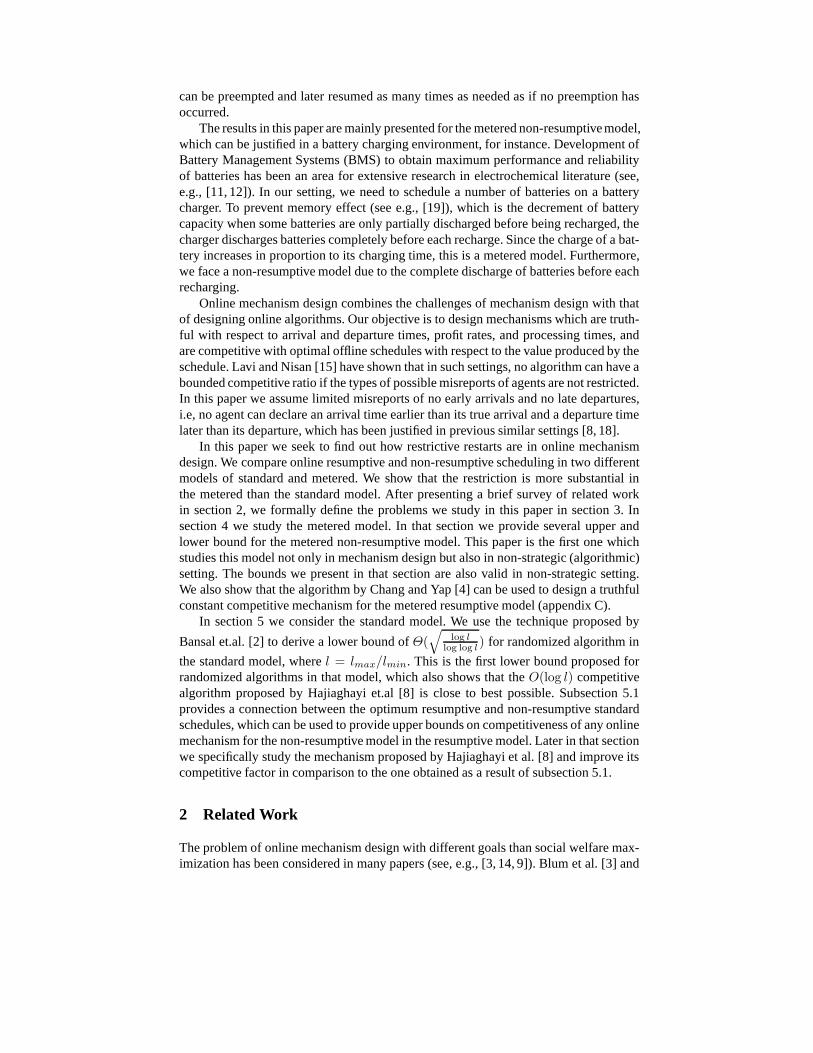
Proof. From now on we only consider jobs allocated inOPT and not inALG. Forma bipartite graphG = (V = (V l, V r), E) by adding a nodevlj in V l for every jobjand a nodevri in V r for every intervali in [I1, I2, . . . , In]. Add an edge with unlimitedcapacity from every nodevlj to all nodesvri if and only if j ∈ Ji. Add a nodes and

connect it by an edge of weightloptj to every nodej in V l and a nodet and connectevery node inV r to t by weight 1. If we can show that the minimum cut ofG hasweight

∑kj=1 l

optj , from the max-flow min-cut theorem we conclude that there is aflow

of weight∑k

j=1 loptj in G. Let fji be the flow fromvlj to vri in maximum flow of graph

G. By settingsji = fji/loptj , all the previously stated conditions will be satisfied. The

following lemma shows this is true.

Lemma 2. The minimum cut ofG has weight∑k

j=1 loptj .

Proof. Prove by contradiction. Suppose that there exists a cutC in G with weight|C| <∑k

j=1 loptj . As shown in figure 1, let the cut separateS = s, J, I fromT = t, J ′, I ′

and have weightw where

w =∑

j∈J′

loptj + |I| <∑

j∈J∪J′

loptj ⇒ |I| <∑

j∈J

loptj

Let d the period from beginning of the allocation of first job inJ to the end ofthe allocation of the last job inJ . We have|I| < ∑

j∈J loptj ≤ |d|. We know thatdcontains no interval outsideI (otherwise there would be an edge of weight∞ from StoT ). But for any intervald, the set of intervals included in it,Id, satisfies the followinginequality:3|d| − 2 ≤ |Id|. We also know that the arrival-departure interval of each jobhas length at least 1, so|d| ≥ 1. We conclude that|d| ≤ 3|d| − 2 ≤ |Id| ≤ |I|. Thelast inequality followed from the fact thatd contains no interval not inI, and therefore,the set of intervals contained ind, Id is a subset ofI. This contradicts our previousinequality,|I| < |d|.

∞∞

∞

21

lopt1

s

t

1 1 1

lopt2

lopt

k

∞

1 2

C

J

I I ′

J ′

n

k

Fig. 1.GraphG in proof of lemma 2

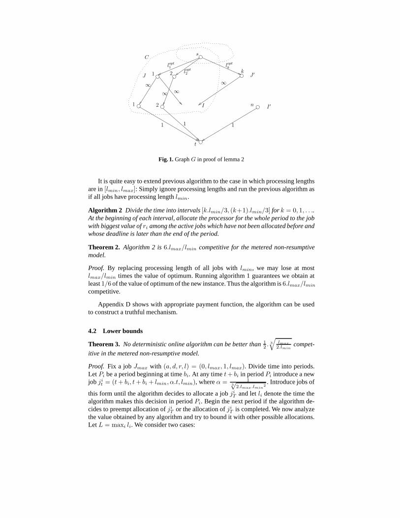
It is quite easy to extend previous algorithm to the case in which processing lengthsare in[lmin, lmax]: Simply ignore processing lengths and run the previous algorithm asif all jobs have processing lengthlmin.

Algorithm 2 Divide the time into intervals[k.lmin/3, (k+1).lmin/3] for k = 0, 1, . . ..At the beginning of each interval, allocate the processor for the whole period to the jobwith biggest value ofri among the active jobs which have not been allocated before andwhose deadline is later than the end of the period.

Theorem 2. Algorithm 2 is6.lmax/lmin competitive for the metered non-resumptivemodel.

Proof. By replacing processing length of all jobs withlmin, we may lose at mostlmax/lmin times the value of optimum. Running algorithm 1 guarantees we obtain atleast1/6 of the value of optimum of the new instance. Thus the algorithm is6.lmax/lmin

competitive.

Appendix D shows with appropriate payment function, the algorithm can be usedto construct a truthful mechanism.

4.2 Lower bounds

Theorem 3. No deterministic online algorithm can be better than12 .

3

√

lmax

2.lmincompet-

itive in the metered non-resumptive model.

Proof. Fix a jobJmax with (a, d, r, l) = (0, lmax, 1, lmax). Divide time into periods.LetPi be a period beginning at timebi. At any timet+ bi in periodPi introduce a newjob jit = (t+ bi, t+ bi + lmin, α.t, lmin), whereα = 1

3√

2.lmax.lmin2. Introduce jobs of

this form until the algorithm decides to allocate a jobjiT and letli denote the time thealgorithm makes this decision in periodPi. Begin the next period if the algorithm de-cides to preempt allocation ofjiT or the allocation ofjiT is completed. We now analyzethe value obtained by any algorithm and try to bound it with other possible allocations.LetL = maxi li. We consider two cases:

1.L ≤ α.lmax.lmin. In this case the algorithm obtains value at mostL+α.∑

i li.lmin ≤L+α.lmax.lmin from allocating the last job in each period and the longest allocation ofJmax with lengthL. In this case another possible solution is to begin allocatingJmax

at time 0 and never to preempt it. This solution has valuelmax. In this case the ratio ofoptimal to produced solution is at least:

lmax

L+ α.lmax.lmin≥ lmax

2.α.lmax.lmin=

1

2.α.lmin=

1

2. 3

√

lmax

2.lmin

2. L ≥ α.lmax.lmin. The value obtained by the algorithm is still not more thanL + α.lmax.lmin. Whereas one may decide to never allocateJmax and preempt theallocation for the new job whenever one job arrives. The value obtained by this scheduleis at least

∫ li0 α.t.dt in each intervali. Total value is the sum of these values over all

intervals. The ratio of this value to the produced value (by the algorithm) is

L2.α/2

L+ α.lmax.lmin≥ L2.α/2

2.L≥ α2.lmax.lmin

4=

1

2. 3

√

lmax

2.lmin

This is true even if we only consider the value obtained in intervalargmaxi li.

Theorem 4. No deterministic online algorithm can be(1−α).rmax/rmin competitivefor anyα > 0 in the metered non-resumptive model (appendix F).

Theorem 5. No deterministic online algorithm for casermin = rmax can be betterthan

√2-competitive in the metered non-resumptive model (appendix F).

5 The Standard Model

In appendix H we use the technique proposed by Bansal et al. [2] to derive a lower

bound ofΘ(√

log llog log l ) on any randomized algorithm in the standard model, wherel =

lmax/lmin. This bound is valid for both resumptive and non-resumptivemodels sincein the proof, the option of rescheduling a previously preempted job is never considered.The connection between resumptive and non-resumptive versions of the standard modelcan be seen in other results too. There exist a deterministiclower bound of(1 +

√k)2

which applies for both the resumptive and non-resumptive standard models [18]. Insubsection 5.1 we prove that any constant competitive algorithm for the non-resumptivemodel is also constant competitive in the resumptive model for scheduling jobs of unitlength. A direct consequence of this result is 10-competitiveness of a mechanism in [8]for the resumptive model which was originally proposed as a 5-competitive mechanismfor the non-resumptive model. In subsection 5.2 we present atighter analysis of thealgorithm and prove its 7.75-competitiveness. Note that Porter’s mechanism, if used forscheduling unit-length jobs, guarantees a competitive ratio of (1+

√

rmax/rmin)2+1.

5.1 Resumption vs. restarts in the standard model

In this section we compare resumptive and non-resumptive algorithms in the standardmodel for the special case of jobs with equal length of processing time. We begin withthe definition of value of a schedule in the resumptive and non-resumptive models. LetVnr(s) be the value of schedules in the non-resumptive standard model andVr(s) beits value in the resumptive standard model.

Hajiaghayi et al. [8] proposed a truthful mechanism which is5-competitive in thenon-resumptive model. I.e. for every profile of playersθ,Vnr(MEC(θ)) ≤ Vnr(OPTnr(θ)) ≤5.Vnr(MEC(θ)), whereMEC(θ) is the schedule produced by mechanism in [8] andOPTnr(θ) is the optimum schedule in the non-resumptive model.

The value of a schedule in the non-resumptive model cannot bemore than its valuein the resumptive model, i.e. we haveVr(s) ≥ Vnr(s) for every schedules. This holdsfor the optimum schedule of the non-resumptive model,V OPT

r (θ) = Vr(OPTr(θ)) ≥Vr(OPTnr(θ)) ≥ Vnr(OPTnr(θ)) = V OPT

nr (θ). We seek relations of the formV OPTr (θ) ≤

C(θ).V OPTnr (θ), for in this case we haveV OPT

r (θ) ≤ 5.C(θ).Vnr(MEC(θ)) ≤ 5.C(θ).Vr(MEC(θ)).In particular ifC(θ) = c for all θ, the mechanism in [8] would be5c-competitive in theresumptive model.

In what follows, we show that such a constant exists and its value is 2, which im-mediately results that mechanism in [8] is (at most) 10-competitive in the resumptivemodel. Note that the optimum solution in the non-resumptivemodel is equal to theoptimum solution of the non-preemptive model.

Definition 3. Let the height of a set of jobs,h, in a schedulings be the maximum ofk forwhich there exists jobsj1,...,jk wherebj1 < bj2 < ... < bjk andej1 > ej2 > ... > ejk .

Definition 4. Let the time in which jobi begins receiving service (in a schedulings,which would be defined in the context) bebi. Let the time in which the jobi finishesreceiving service (and is never allocated again) beei.

Lemma 3. For any preemptive schedulings, there exists a preemptive schedulings′

with Vr(s) = Vr(s′) where ifbi < bj for any two jobsi andj andei > bj (in s′), then

ei > ej . Alsoi is not allocated in[bj , ej].

Proof. For the first part consider a schedulings as in Figure 2.a. As long as the twojobs have a form shown in the figure, their allocation can be exchanged (as shown byarrows) without affecting other jobs. Notice that new allocations are feasible since theallocation periods are in[bi, ei] for eachi.

bi

bj ej

ei bi

bj ej

ei

Fig. 2. proof of lemma 3

To prove the second part, consider two jobs as in figure 2.b. The allocation of thesejobs can also be exchanged as shown by arrows without affecting other jobs.

We conclude that there exists an optimal resumptive schedule in which allocation ofjobs form a parenthesis expression and jobs are not allocated in [bi, ei] for each of theirinner jobsi.

Theorem 6. For any schedulings of n jobs, there exists a schedulings′ of these jobswith value2.Vnr(s

′) ≥ Vr(s) in the standard model.

Proof. Claim. for any scheduling of jobs with heighth and size (the number of jobs)kandV = Vr(s):

1. If k is even: There exists a schedulings′ with Vnr(s′) ≥ V/2 which usesk/2 of

the jobs.2. If k is odd: There exists a schedulings′ which uses(k + 1)/2 of the jobs and a job

m whereV − v(m) ≤ (Vnr(s′)− v(m)).2 andm is allocated ins′. I.e. if we omit

m from both allocations, the non-resumptive value ofs′ is still more than half ofthe resumptive value ofs.

Base: forh = 1, if k is odd select the biggest(k − 1)/2 jobs and letm be the(k + 1)/2th biggest job. Otherwise selectk/2 biggest jobs.

For h = 2, if k is odd (k + 1 is even) select biggest(k + 1)/2 from j1, ..., jk, j.Otherwise, selectk/2 biggest fromj1, ..., jk, j and letm be the(k + 1)/2th biggestelement.

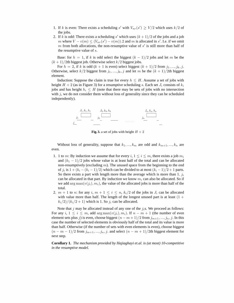
Induction: Suppose the claim is true for everyh ≤ H . Assume a set of jobs withheightH + 2 (as in Figure 3) for a resumptive schedulings. Each setJi consists ofkijobs and has heighthi ≤ H (note that there may be sets of jobs with no intersectionwith j, we do not consider them without loss of generality since they can be scheduledindependently).

j2j1 jn

j

J2, k2, h2J1, k1, h1 Jn, kn, hn

Fig. 3. a set of jobs with heightH + 2

Without loss of generality, suppose thatk1, ..., km are odd andkm+1, ..., kn areeven.

1. 1 tom: By induction we assume that for everyi, 1 ≤ i ≤ m, there exists a jobmi

and(k1 − 1)/2 jobs whose value is at least half of the total and can be allocatednon-resumptively (excludingm). The unused space from the beginning to the endof ji is 1+ (ki − (ki − 1)/2) which can be divided to at most(ki − 1)/2+ 1 parts.So there exists a part with length more than the average whichis more than 1.jican be allocated in that part. By induction we knowmi can also be allocated. So ifwe addargmax(v(ji),mi), the value of the allocated jobs is more than half of thetotal.

2. m + 1 to n: for any i, m + 1 ≤ i ≤ n, ki/2 of the jobs inJi can be allocatedwith value more than half. The length of the longest unused part is at least(1 +ki/2)/(ki/2 + 1) which is 1. Soji can be allocated.

Note thatj may be allocated instead of any one of thejis. We proceed as follows:For anyi, 1 ≤ i ≤ m, addargmax(v(ji),mi). If n − m + 1 (the number of evenelement sets plusj) is even, choose biggest(n−m+1)/2 from jm+1, ..., jn, j. In thiscase the number of selected elements is obviously half of thetotal and its value is morethan half. Otherwise (if the number of sets with even elements is even), choose biggest(n − m − 1)/2 from jm+1, ..., jn, j. and select(n − m + 1)/2th biggest element fornext step.

Corollary 1. The mechanism provided by Hajiaghayi et.al. is (at most) 10-competitivein the resumptive model.

5.2 7.75-competitiveness of the mechanism

Here we prove the 7.75-competitiveness of mechanism proposed in [8].Mechanism 1 [8]: Call a point in time critical if an allocation in completed or a

new agent arrives. At each critical timet, compare the value of the agents present andallocate the agent with highest value. There may be one agentwhich was being allocatedin the period ended att, with the service lengthδ ≤ 1. Multiply the value of this agent byαδ (α is a constant to be determined). Collect from every winning agent the minimumvalue for which it would still be a winning agent.

Theorem 7. Mechanism 1 is 7.75 competitive for efficiency forα = 2.25 in the stan-dard resumptive model.

Proof. Use a charging analysis. We compare the value ofOPT , the optimum schedul-ing for our model, andMEC, the scheduling produced by mechanism 1. For each jobiallocated inOPT , lethi be the time the allocation ofi reaches 1/2. Letmi behi−1/2.If an agent allocated inOPT is also allocated inMEC, charge its value to itself. Oth-erwise, charge the value of eachi to the first job completed in a chain which is presentin MEC at timemi.

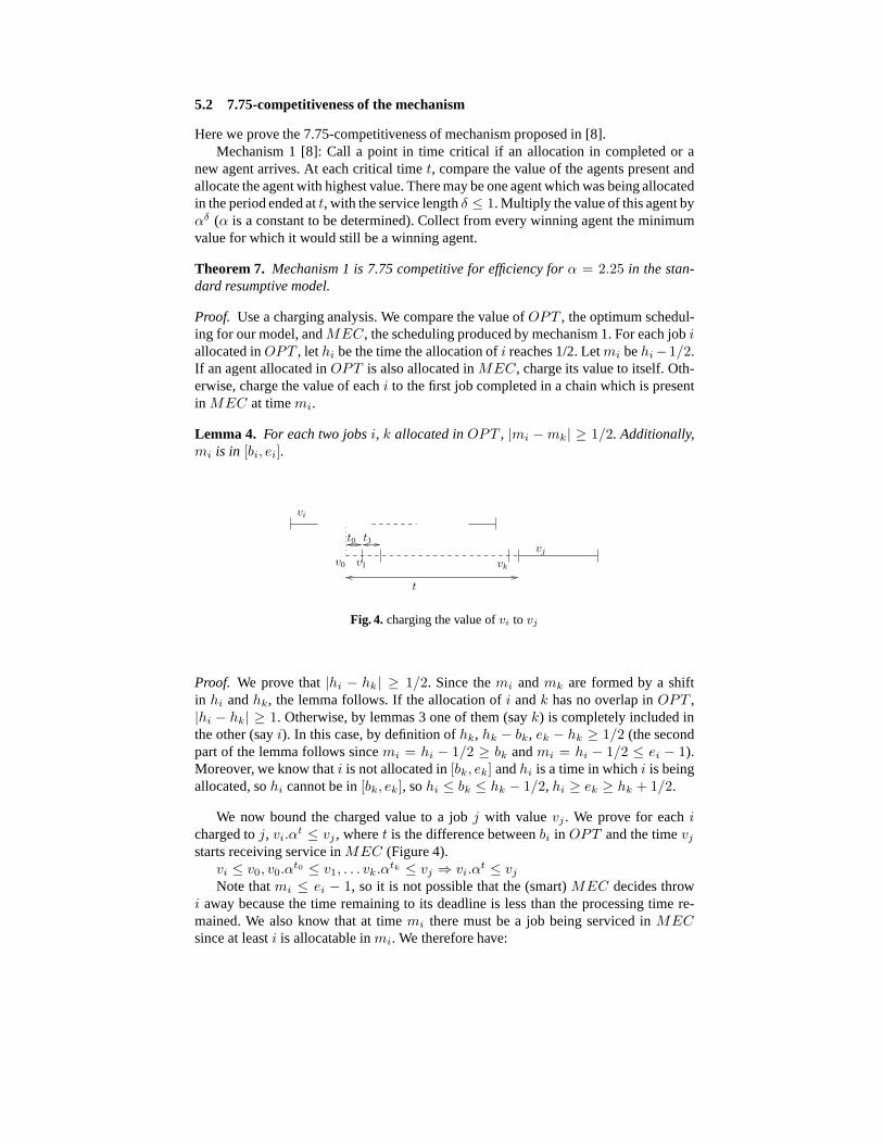
Lemma 4. For each two jobsi, k allocated inOPT , |mi −mk| ≥ 1/2. Additionally,mi is in [bi, ei].

vi

t

v1 vk

vjt1t0

v0

Fig. 4. charging the value ofvi to vj

Proof. We prove that|hi − hk| ≥ 1/2. Since themi andmk are formed by a shiftin hi andhk, the lemma follows. If the allocation ofi andk has no overlap inOPT ,|hi − hk| ≥ 1. Otherwise, by lemmas 3 one of them (sayk) is completely included inthe other (sayi). In this case, by definition ofhk, hk − bk, ek − hk ≥ 1/2 (the secondpart of the lemma follows sincemi = hi − 1/2 ≥ bk andmi = hi − 1/2 ≤ ei − 1).Moreover, we know thati is not allocated in[bk, ek] andhi is a time in whichi is beingallocated, sohi cannot be in[bk, ek], sohi ≤ bk ≤ hk − 1/2, hi ≥ ek ≥ hk + 1/2.

We now bound the charged value to a jobj with valuevj . We prove for eachicharged toj, vi.αt ≤ vj , wheret is the difference betweenbi in OPT and the timevjstarts receiving service inMEC (Figure 4).

vi ≤ v0, v0.αt0 ≤ v1, . . . vk.α

tk ≤ vj ⇒ vi.αt ≤ vj

Note thatmi ≤ ei − 1, so it is not possible that the (smart)MEC decides throwi away because the time remaining to its deadline is less than the processing time re-mained. We also know that at timemi there must be a job being serviced inMECsince at leasti is allocatable inmi. We therefore have:

The value charged toj is at mostvj .(α+α1/2+α0+...) = vj .(α+(α+α3/2)/(α−1)), whose optimal value is6.75.vj whenα = 2.25. Adding the value ofvj to itself forthe case it is present in bothOPT andMEC, we conclude that this mechanism is (atmost) 7.75-competitive.

Theorem 8. Mechanism 1 is truthful in the standard resumptive model (see appendixI).

References

1. M. Babaioff, N. Immorlica, and R. Kleinberg. Matroids, secretary problems, and onlinemechanisms. InSODA ’07, pages 434–443. Society for Industrial and Applied Mathematics,2007.

2. N. Bansal, N. Chen, N. Cherniavsky, A. Rudra, B. Schieber,and M. Sviridenko. Dynamicpricing for impatient bidders. InSODA ’07, pages 726–735. Society for Industrial and Ap-plied Mathematics, 2007.

3. A. Blum, V. Kumar, A. Rudra, and F. Wu. Online learning in online auctions. InSODA ’03,pages 202–204. Society for Industrial and Applied Mathematics, 2003.

4. E.-C. Chang and C. Yap. Competitive online scheduling with level of service.J. of Schedul-ing, 6(3), Oct. 2003. Special Issue on Online Algorithms.

5. F. Y. L. Chin and S. P. Y. Fung. Improved competitive algorithms for online scheduling withpartial job values.Theor. Comput. Sci., 325(3):467–478, 2004.

6. M. Chrobak, L. Epstein, J. Noga, J. Sgall, R. van Stee, T. Tichy, and N. Vakhania. Preemp-tive scheduling in overloaded systems. InICALP ’02, pages 800–811, London, UK, 2002.Springer-Verlag.

7. E. B. Dynkin. The optimum choice of the instant for stopping a markov process.SovietMath. Dokl, 0(4):627–629, 1963.

8. M. T. Hajiaghayi, R. Kleinberg, M. Mahdian, and D. C. Parkes. Online auctions with re-usable goods. InEC ’05: Proceedings of the 6th ACM conference on Electronic commerce,pages 165–174. ACM, 2005.

9. M. T. Hajiaghayi, R. Kleinberg, and D. C. Parkes. Adaptivelimited-supply online auctions.In EC ’04: Proceedings of the 5th ACM conference on Electronic commerce, pages 71–80.ACM, 2004.

10. M. T. Hajiaghayi, R. D. Kleinberg, and T. Sandholm. Automated online mechanism designand prophet inequalities. InAAAI, pages 58–65, 2007.

11. A. Jossen, V. Spth, H. Dring, and J. Garche. Reliable battery operation a challenge for thebattery management system.Journal of Power Sources, 84:283–286, 1999.

12. R. Kaiser. Optimized battery-management system to improve lifetime in renewable energysystems.Journal of Power Sources, 168:58–65, 2007.

13. R. Kleinberg. A multiple-choice secretary algorithm with applications to online auctions.In SODA ’05: Proceedings of the sixteenth annual ACM-SIAM symposium on Discrete algo-rithms, pages 630–631. Society for Industrial and Applied Mathematics, 2005.

14. R. Kleinberg and T. Leighton. The value of knowing a demand curve: Bounds on regret foronline posted-price auctions. InFOCS ’03, page 594. IEEE Computer Society, 2003.

15. R. Lavi and N. Nisan. Online ascending auctions for gradually expiring items. InSODA ’05,pages 1146–1155. Society for Industrial and Applied Mathematics, 2005.

16. J. W. S. Liu, K.-J. Lin, W.-K. Shih, A. C. shi Yu, J.-Y. Chung, and W. Zhao. Algorithms forscheduling imprecise computations.Computer, 24(5):58–68, 1991.

17. N. Nisan and A. Ronen. Algorithmic mechanism design.Games and Economic Behavior,35:166–196, 2001.

18. R. Porter. Mechanism design for online real-time scheduling. In EC ’04: Proceedings of the5th ACM conference on Electronic commerce, pages 61–70. ACM, 2004.

19. Y. Sato, S. Takeuchi, and K. Kobayakawa. Cause of the memory effect observed in alkalinesecondary batteries using nickel electrode.Journal of Power Sources, 93:20–24, 2001.

6 Appendixes

A rmax/rmin + 1 competitive algorithm for the non-resumptivemodel

Algorithm 3 At the end of any busy period, select the job with highest profit rate amongactive jobs. Continue the allocation without preemption until either the job is completedor its deadline is reached.

Theorem 9. Algorithm 3 isrmax/rmin +1 competitive in the metered non-resumptivemodel.

Proof. Note that as in the previous algorithm, any job scheduled inALG is never con-sidered for allocation later, so any timet in which the processor is busy inALG isvaluable.

Any job is allocated in at most one continuous period of time in OPT (let theprocessor be idle at any time not in last period of allocationof some job). Consider anytime t in which the processor is busy inOPT processing jobi. If the processor is alsobusy inALG with job j, chargeri to time t in ALG, where the charged profit rate isat mostrmax/rmin times the profit rate oft in ALG. Now suppose that processor isbusy in period[tb, tb + l] in OPT processing jobi but idle in this period inALG. Bythe definition of the algorithm,i can not be active attb since otherwise it would havebeen allocated. We also know thatdi > tb since this job is allocated attb in OPT . Thismeans thati has been allocated inALG and its allocation was completed beforetb. Thelength of the allocation inALG [t′b, t

′b + l′] is thereforel′ = li ≥ l. Chargeri to every

time in [t′b, t′b + l].

One can see that the charged value is equal to the value ofOPT and every busytime t in ALG is charged at mostrmax/rmin + 1 times of its value inALG.

Appendix D shows with appropriate payment function, the algorithm can be usedto construct a truthful mechanism.

B Randomized algorithms

In this section we use deterministic algorithms for specialcases of equal profit rates andbounded processing times proposed in previous sections to present two randomizedalgorithms which areO(log(lmax/lmin)) andO(log(rmax/rmin)) competitive. Thetwo algorithms are based on the technique of ”classify and randomly select” (see, e.g.,[8]).

Algorithm 4 Suppose that every job has a processing time in[lmin, lmax]. GuessL, arandom power of 2 in[lmin, 2.lmax]. Ignore any job with processing time less thanLand treat every other job as if their processing time isL (notice that a solution to the newproblem is valid for the original problem with possibly lessvalue). Use the deterministicalgorithm for equal processing times proposed in previous section to schedule jobs.

Theorem 10. Algorithm 4 isO(log(lmax/lmin)) competitive in the metered non-resumptivemodel.

Algorithm 5 Suppose that every job has a value rate in[rmin, rmax]. GuessR, a ran-dom power of 2 in[rmin, 2.rmax]. Ignore every jobi of valueri < R and treat everyother job as if its value isR. Use the algorithm 2 to find an allocation for jobs withequal processing rates.

Theorem 11. Algorithm 5 isO(log(rmax/rmin)) competitive in the metered non-resumptivemodel.

Appendix E shows with appropriate payment function, the algorithm can be used toconstruct a truthful mechanism.

C The metered resumptive model

We now consider the metered resumptive model and show that although no algorithmcould be constant competitive in the metered non-resumptive model, there are truthfulconstant competitive mechanisms for the metered resumptive model.

Algorithm 6 ([4]) At any time allocate the processor to the active job with highestprofit rate.

Theorem 12. ([4]) Algorithm 6 is 2-competitive in the metered resumptive model.

Appendix G shows with appropriate payment function, the algorithm can be usedto construct a truthful mechanism.

D Truthfulness of O(lmax/lmin) and rmax/rmin+1 mechanisms

Definition 5. Defineµi(s) = 1 if i wins an allocation (of lengthlmin/3) in schedules and zero otherwise. Definerci (θ) = minr µi(f((ai, di, r, li), θ−i)) = 1 as the criticalvalue of agenti on a profile of typesθ and an allocation rulef : Θk → S. We caninterpret the critical value as the minimum profit rate an agent can declare and still bea winning agent.

Theorem 13. The mechanism(f, pi), i = 1, 2, . . . , k, wheref is the allocation rule ofalgorithm 2 andpi(θ) = µi(f(θ)).r

ci (θ).lmin/3 is a truthful mechanism in the metered

non-resumptive model. This mechanism satisfies individualrationality and never paysa winning agent.

Proof. Before we proceed to prove the theorem considering different parameters, Weshould note that the knowledge about the value oflmin is a prerequisite for the perfor-mance of the algorithm, i.e, this is not a value that the mechanism learnsby observingthe inputs. Therefore, we can assume that no agent can declare a processing time lessthanlmin.

We first prove truthfulness with respect to arrival, departure, and processing times.Suppose that agenti hasθi = (ai, di, ri, li) and bidsθ′i = (a′i, d

′i, r

′i, l

′i). First observe

that the produced schedule does not change by bidding anyl′i ≥ li. This is becauseneither being considered for allocation at the beginning ofan interval, nor its allocationtime (which is a constantlmin/3 if allocated) is affected by the value ofl′i. The agent’spayment is also independent of declared length of processing time.

Now consider the case that the agent announcesd′i ≤ di. LetIlast be the last intervalwhose deadline is not afterd′i. This is the last intervali would be considered to beallocated in when the agent bidsd′i. Note that the schedule in cases of biddingdi or d′idoes not change until the end ofIlast. Thereforei would not be allocated by announcingd′i if it had not been allocated by announcingdi. Next observe thatrci (θ

′) ≥ rci (θ),whereθ′ = θ except in the deadline of agenti, since anyr that would makei to beallocated in[a′i, d

′i] would also make it allocated in[a′i, di]. This means that the agent’s

payment does not decrease by biddingd′i. We conclude that the agent has no incentiveto bidd′i.

We will now show that the agent would not benefit by biddingθ′i = (a′i, di, r′i, li)

instead ofθi = (ai, di, r′i, pi), wherea′i > ai. As in the previous case, the agent’s

payment would not decrease by biddingθ′i. We therefore only need to show that theagent would not be allocated by biddingθ′i if it would not be allocated by biddingθi.Note that the existence of a job at a timet does not affect jobs with higher profit rates.Therefore the state of the mechanism with respect to jobs with value more thanr′i doesnot change at timea′i whetheri declaresa′i or ai. This means that the allocation ofiaftera′i would be the same in both cases. Therefore if the agent is allocated at a timemore thana′i by declaringa′i, it would have still been allocated by declaringai.

It only remains to show that the agent gains nothing by declaringθ′i = (ai, di, r′i, pi)

instead ofθi = (ai, di, ri, pi). If the agent does not win by declaringθi, this is becauseri < rci (θ). The agent only wins by declaringr′i ≥ rci (θ) in which case its utility wouldberi.lmin/3 − rci (θ).lmin/3 < 0. If the agent wins by biddingθi, by the definition ofpayment functions its utility would be non-negative, whichwould drop to zero if it bidsanyr′i < rci (θ).

Individual rationality follows from the fact that for any winning agent we haveri >rci (θ). Also sincerci (θ) > 0 for any agent, we conclude that no agent is paid money bythe mechanism.

Theorem 14. The mechanism(f, pi), i = 1, 2, . . . , k, wheref is the allocation rule

of algorithm 3 andpi(θ) = ri.Li(ri) −∫ ri0

Li(x).dx (for an agent with nonzero allo-cation) is a truthful mechanism in the metered non-resumptive model, whereLi(r) isthe allocation length of agenti if it declares profit rater, fixing θ−i. This mechanismsatisfies individual rationality and never pays an agent.

l

r

L′

i

Li

L′′

il′′i

l′i

li

Fig. 5.The load function of agenti regarding different declared processing lengths

Proof. LetL′i(r) be a the allocation length of agenti when it declares type(a′i, d

′i, r, l

′i).

First we show that such function is a non-decreasing function. We need to show thatthe allocation length of an agent does not decrease when it declaresr′ ≥ r. Assumefor contradiction that this is true and the agent wins allocation length ofl at timetwwhen declaringr and allocation length ofl′ < l at time t′w when declaringr′ ≥ r.Note thatt′w ≤ tw since the agent who wins attw by declaringr will still win atthat time by declaring any value more thanr. The allocation of an agent winning att is min(t + l′i, d

′i) − t, and using the fact thatt′w ≤ tw we conclude that the agents

allocation when declaringr′ (and winning att′w) cannot be less than its allocation whendeclaringr (and winning attw).

Using this fact we prove truthfulness with respect to different parameters. We firstshow truthfulness with respect to declared profit rate and processing length simultane-ously, i.e, we show that the utility of the agent declaring(a′i, d

′i, r

′i, l

′i) is not more than

its utility when it declares(a′i, d′i, ri, li).

Let Li(r) the allocation length of agenti when it declares type(a′i, d′i, r, li). We

consider two cases:1. l′i ≤ li: The agent’s utility when declaringr′i andl′i isu′ = ri.L

′i(r

′i)−(r′i.L

′i(r

′i)−

∫ r′i0 L′

i(x).dx). The agent would have utilityu = ri.Li(ri)−(ri.Li(ri)−∫ ri0 Li(x).dx) =

∫ ri0 Li(x).dx if it declaresri andli. Suppose for contradiction thatu′ > u. Notice also

that for anyr, we haveLi(r) ≥ L′i(r). We can write:

ri.L′i(r

′i)− (r′i.L

′i(r

′i) −

∫ r′i

0

L′i(x).dx

>

∫ ri

0

Li(x).dx

→ I = (ri − r′i).L′i(r

′i) >

∫ ri

0

Li(x).dx

−∫ r′i

0

L′i(x).dx = II

a. r′i ≤ ri: In this case using the fact that∀x, Li(x) ≥ L′i(x) we can write

∫ ri0

Li(x).dx−∫ r′i0 L′

i(x).dx ≥∫ rir′i

Li(x).dx, which is not less than(ri−r′i).Li(r′i) since we know

Li(r) is a non-decreasing function andr′i ≤ ri. Using the fact thatLi(r) ≥ L′i(r)

we conclude(ri − r′i).Li(r′i) ≥ (ri − r′i).L

′i(r

′i). As a resultI ≤ II which contra-

dicts equation 1.

b. r′i > ri: Form Li(r) ≥ L′i(r) we know that

∫ ri0

Li(x).dx −∫ r′i0

L′i(x).dx ≥

∫ ri0 L′

i(x).dx −∫ r′i0 L′

i(x).dx which is equal to∫ rir′i

L′i(x).dx = −

∫ r′iri

L′i(x).dx.

SinceL′i(r) is a non-decreasing function, we can write−

∫ r′iri

L′i(x).dx ≥ −(r′i −

ri).L′i(r

′i) = (ri − r′i).L

′i(r

′i), which is a contradiction of equation 1.

2. l′i > li. In this case note that the valuation of an agent would not be more thanri.li even if its allocation length exceedsli.The agent’s utility therefore would beu′ =

ri.min(li, L′i(r

′i))−(r′i.L

′i(r

′i)−

∫ r′i0 L′

i(x).dx) = ri.Li(r′i)−r′i.L

′i(r

′i)+

∫ r′i0 L′

i(x).dx ≤ri.Li(r

′i) − r′i.Li(r

′i) +

∫ r′i0

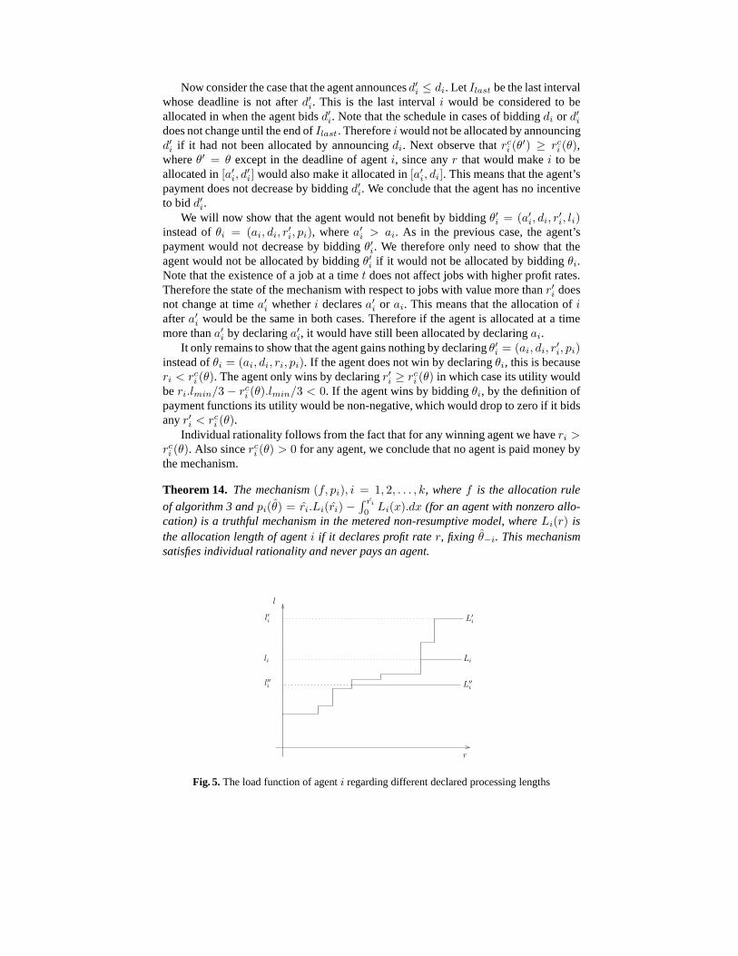
Li(x).dx = u. Whereu is the agnet’s utility when declar-ing its processing length truthfully. The last inequality is due to the fact that the agentspayment can only increase if it increases its processing time (Figure 5).

Having proved truthfulness of mechanism w.r.t profit rates and processing times,we analyze utility of an agent and show that the utility does not increase when an agentdeclares[a′i, d

′i], di ≥ d′i instead of[a′i, di]. Suppose thatLi(r) is a function which spec-

ifies allocation ofi when it declares(a′i, di, r, li) andL′i(r) is a function which specifies

allocation ofi when it declares(a′i, d′i, r, li). Suppose that the agent wins allocation at

timetw < di declaringri anddi, with allocation lengthLi(ri) = min(tw+ li, di)−tw.If d′i < tw, the agent does not win andL′

i(ri) = 0. If tw ≤ d′i, the agent would stillwin at timetw, where its allocation length would beL′

i(ri) = min(tw + li, d′i) − tw

which is not more than its allocation length in case it bids truthfully. In both cases wehaveL′

i(r) ≤ Li(r). We conclude that∫ ri0 Li(x).dx, the utility of the agent biddingdi,

is not less than∫ ri0

L′i(x).dx, its utility when it bidsd′i.

l

r

li

Li(r)

L′

i(r)

Rn+1Rn

Fig. 6.The load function of agenti regarding different declared arrival times

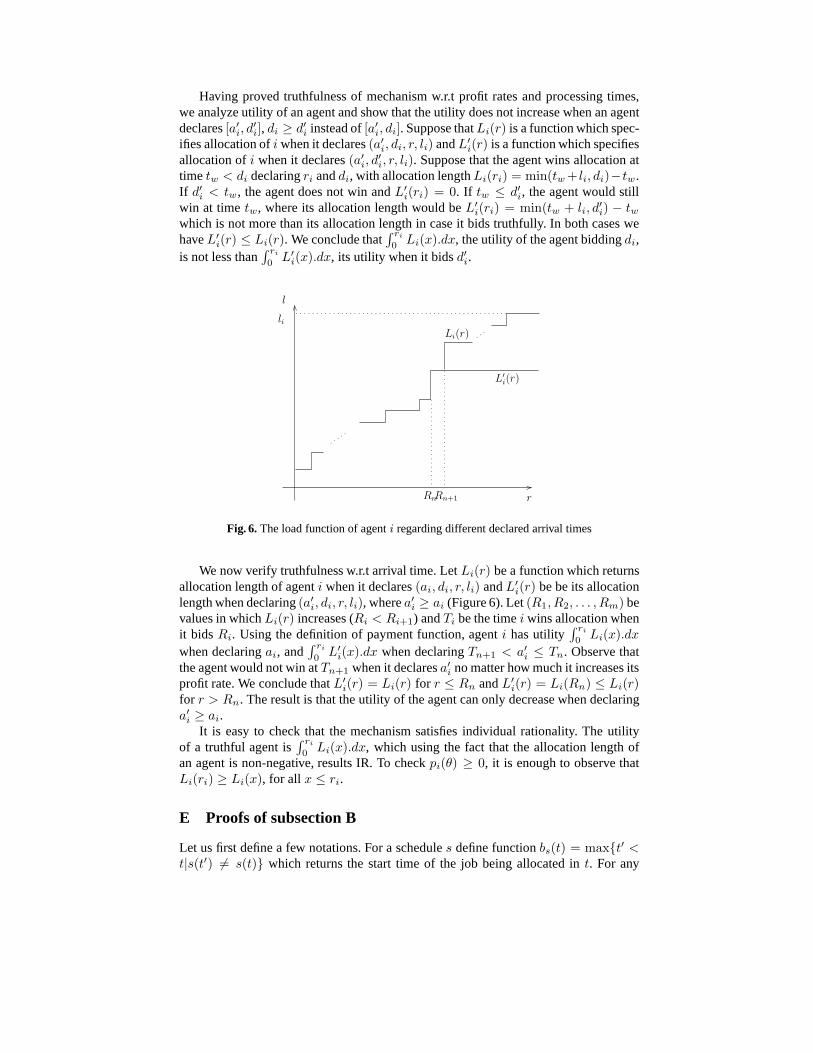
We now verify truthfulness w.r.t arrival time. LetLi(r) be a function which returnsallocation length of agenti when it declares(ai, di, r, li) andL′

i(r) be be its allocationlength when declaring(a′i, di, r, li), wherea′i ≥ ai (Figure 6). Let(R1, R2, . . . , Rm) bevalues in whichLi(r) increases (Ri < Ri+1) andTi be the timei wins allocation whenit bids Ri. Using the definition of payment function, agenti has utility

∫ ri0 Li(x).dx

when declaringai, and∫ ri0

L′i(x).dx when declaringTn+1 < a′i ≤ Tn. Observe that

the agent would not win atTn+1 when it declaresa′i no matter how much it increases itsprofit rate. We conclude thatL′

i(r) = Li(r) for r ≤ Rn andL′i(r) = Li(Rn) ≤ Li(r)

for r > Rn. The result is that the utility of the agent can only decreasewhen declaringa′i ≥ ai.

It is easy to check that the mechanism satisfies individual rationality. The utilityof a truthful agent is

∫ ri0 Li(x).dx, which using the fact that the allocation length of

an agent is non-negative, results IR. To checkpi(θ) ≥ 0, it is enough to observe thatLi(ri) ≥ Li(x), for all x ≤ ri.

E Proofs of subsection B

Let us first define a few notations. For a schedules define functionbs(t) = maxt′ <t|s(t′) 6= s(t) which returns the start time of the job being allocated int. For any

schedules, real valuel, and set of jobsJ defines(J, l) as a schedule which is idle atany timet wheres(t) = j /∈ J or s(t) = j ∈ J but t − bs(t) > l, and equal tosotherwise. Lets(J) = s(J,∞). The proofs of the following theorems are moved toappendix E.

Proof of theorem 10: We can view the randomized algorithm as an algorithm whichdecides randomly to solve a problem using a deterministic algorithm from a set ofpossible problems (to be defined formally). LetOPT be the set of jobs allocated inoptimal schedulesOPT . Let (l1, l2, . . . , lm) be the sequence of all powers of 2 between[lmin, 2.lmax] (let l0 = lmin) andOPTi be the subset ofOPT consisting of jobs withrequired processing length in[li, li+1]. Let P (L = li) be the problem of schedulingjobs with processing time not less thanli as if they had processing timeli (and ignoringrest of the jobs). First observe thats(OPTi, li) is a feasible solution forP (L = li) andthus, using a 6-competitive mechanism to solveP (L = li), we would obtain a valueat leastv(s(OPTi, li))/6 ≥ v(s(OPTi))/12, where the latter inequality is becausethe allocation length of each job ins(OPTi) is at most twice as big as its allocationlength ins(OPTi, li). Our randomized algorithm solves each problemP (L = li) withprobability1/m using a deterministic algorithm. So we can compute the expected valueof our algorithm as follows:

E(v) =1

m.

m∑

i=1

v(s(L = li))

≥ 1

12.m.

m∑

i=1

v(s(OPTi))

=1

12.mv(sOPT )

wheres(L = li) is the schedule produced by the deterministic algorithm forproblemP (L = li). Also noting thatm = O(log(lmax/lmin)) we conclude the theorem. ut

Proof of theorem 11: Let (r1, r2, . . . , rm) be the sequence of all powers of 2 in[rmin, 2.rmax] (let r0 = rmin) andOPTi be the subset ofOPT consisting of jobs withprofit rate in[ri, ri+1]. Let P (R = ri) be the problem of scheduling jobs with profitrate not less thanri as if they had valueri (and ignoring rest of the jobs). First observethat s(OPTi) is a feasible solution ofP (R = ri) and thus, using a 2-competitivemechanism to solveP (R = ri), we would obtain a value at leastv(s(OPTi))/4. Ourrandomized algorithm solves each problemP (R = ri) with probability 1/m usinga deterministic algorithm. So we can compute the expected value of our algorithm asfollows:

E(v) =1

m.

m∑

i=1

v(s(R = ri))

≥ 1

4.m.

m∑

i=1

v(s(OPTi))

=1

4.mv(sOPT )

wheres(R = ri) is the schedule produced by the deterministic algorithm forproblemP (R = ri). Also noting thatm = O(log(rmax/rmin)) we conclude the theorem.

ut

Theorem 15. The mechanism(f, pi), i = 1, 2, . . . , k, wheref is the allocation rule ofalgorithm 2 andpi(θ) = R.Li(R) (for an agent with nonzero allocation) is a truthfulmechanism in the metered non-resumptive model, whereLi(r) is the allocation lengthof agenti if it declares profit rater, fixing θ−i (R is the random choice made by thealgorithm). This mechanism satisfies individual rationality and never pays an agent.

Proof of theorem 15: By declaring any valuer′i < R, the agent does not win anyallocation. So declaring anya′i, d

′i, l

′i does not change the utility of the agent, which is

zero. If the agent declaresr′i ≥ R, the agent is considered for allocation by algorithm 2.The proof of truthfulness of declared values ofa′i, d

′i, andl′i therefore follows directly

from the proof of theorem 9. So we only need to prove truthfulness w.r.t profit rates.Supposing that the agent declares the other parameters truthfully, let Li(r) show

the allocation length of the agent when it declaresr. One can see thatLi(r) = 0 foranyr < R. Additionally, note that the agent’s allocation does not change by declaringanyr′i ≥ R, since the deterministic algorithm treats all jobs as if they had equal profitrates. Any agent who wins by declaring its profit rate truthfully, must haveri ≥ R, andtherefore its utility would beri.Li(R) − R.Li(R) ≥ 0. Such an agent can not changeits payment unless it declaresr′i < R, in which case its utility would drop to zero. Anagent which loses by declaring its profit rate truthfully must haveri < R, and its utilityin case of winning (declaringr′i ≥ R) is r′i.Li(R)−R.Li(R) < 0. ut

F Proof of deterministic lower bounds

Proof of theorem 4: Consider a jobJmin with (a, d, r, l) = (0, 1, rmin, 1). Fix asmall constantt, t < α.rmin/rmax and proceed as follows. Time is divided into peri-ods. Letbi be beginning time of periodPi. Introduce no jobs in[bi, bi + t]. At the timebi+ t, begin a sequence of jobs of the formJ i

h = (bi+ t+h.ε, bi+ t+h.ε+ ε, rmax, ε),for h = 1, 2, . . ., i.e, introduce a new job with profit ratermax and processing lengthε at the deadline of previous job of this form. Stop introducing new jobs at the timethe algorithm decides to allocate a jobJ i

H . Let li be the time the algorithm decides toschedule jobJ i

H in periodPi. Start a new period when the algorithm stops schedulingJ iH (at or before its deadline). LetL = maxi li. First note that any algorithm obtains

valueL.rmin+np.rmax.ε, wherenp is the number of periods. Asε → 0, this value ap-proachesL.rmin asnp cannot approach infinity since it is bounded above bynp ≤ 1/t.The algorithms value is therefore at mostL.rmin.

First consider the case that no period has length more thanτ = rmin/rmax. Thealgorithm therefore obtains a value at mostτ.rmin, whereas another feasible solutionwould be to begin schedulingJmin from time zero and never to preempt it. This solutionhas a valuermin. The ratio of optimal to produced solution’s value in this case is a leastrmin/(τ.rmin) = 1/τ > (1 − α).rmax/rmin.

Now consider the case where there exists a period with lengthmore thanτ . Thealgorithm’s value would still be at mostL.rmin whereas a solution would be to sched-ule all jobs with profit ratermax in the longest period which would have a value at

leastrmax.(L− t). The ratio of optimal to the produced solution is at leastrmax.(L−t)/L.rmin = (1 − t/L).rmax/rmin > (1 − α).rmax/rmin, sincet < α.rmin/rmax

andL > rmin/rmax.We conclude that the algorithm can not have a competitive ratio (1−α).rmax/rmin,

for anyα > 0. ut

Proof of theorem 5: Let Ja be a job with(a, d, r, l) = (0, 1, 1, 0.5). at time0.5− α

introduce a new jobJb = (0.5 − α, 0.5, 1, α) whereα =√2−12 . If the algorithm never

decides to allocateJb, introduce no other job. In this case, the algorithm obtainsa valueof 0.5 from schedulingJa whereas another solution is to scheduleJb in [0.5 − α, 0.5]andJa in [0.5, 1] which has a value0.5 + α. The ratio of optimal to produced solutionis at least

√2.

If the algorithm schedulesJb completely, there are two cases possible. First, thealgorithm decides to go back toJa at some time0.5 ≤ t < 1. In this case introduce anew jobJc = (t + ε, 1, 1, 1 − (t + ε)). Either if the algorithm preemptsJa for Jc orcontinues to completion, it obtains valueα + 1 − t whereas another solution is not toscheduleJa afterJb and only allocateJc with total value0.5−α+α+1− t = 1.5− t.For any0.5 ≤ t < 1, the ratio of optimal to algorithm allocation is at least

√2. Second,

If the algorithm decides to never go back toJa, we introduce no other jobs and thealgorithm obtains valueα whereas optimal value isα + 0.5. In this case also the ratiois more than

√2.

It can be seen that no other choice by the algorithm (preemptingJa for Jb at timemore than0.5− α, schedulingJb in [0.5− α, t] for somet < 0.5) yields better resultsthan the previously considered ones. ut

G Truthfulness of metered resumptive mechanism

Theorem 16. The mechanism(f, pi), i = 1, 2, . . . , k, wheref is the allocation rule

of algorithm 6 andpi(θ) = ri.Li(ri) −∫ ri0 Li(x).dx is a truthful mechanism in the

metered resumptive model, whereLi(r) is the allocation length of agenti if it declaresprofit rater, fixing θ−i.

Proof. We first show that the load functionLi(r) is non-decreasing for any declaredvalue of(a′i, d

′i, r, l

′i). Suppose for contradiction thatLi(r) < Li(r

′) for somer andr′ ≤ r. Let s ands′ be the schedules produced wheni declaresr andr′ respectively,and lett = mint(s

′(t) = i, s(t) 6= i). Let j = s(t) be the job winning the allocation attime t in s. This job must be present ins′ at timet since the two schedules are the sameprior to t. This job has value more thanr and thereforei can not win att with profit rater′ ≤ r.

Using this fact one can easily check truthfulness w.r.t processing length and profitrates with an argument exactly similar to the one in the proofof theorem??.

Using the fact that the agent declares its profit rate and processing length truthfully,we now prove incentive compatibility for declared deadline. Let Li(r) be the agentsallocation when it declares(a′i, di, ri, li) andL′

i(r) be its allocation when it declares(a′i, d

′i, ri, li), d

′i ≤ di. Observe thatL′

i(r) ≤ Li(r) for everyr since the scheduledoes not change befored′i in both cases, and the agent wins no allocation afterd′i if itchanges its deadline tod′i. This shows that the utility of the agent when it bids truthfully,∫ ri0

Li(x).dx can not be less than its utility when it declaresd′i,∫ ri0

L′i(x).dx.

It only remains to prove truthful declaration of arrival times. To check this observethat by changing its arrival-departure interval, an agent can only affect the allocationof agents with profit rates less than its own rate. Lett be the first time the agent winsallocation in the schedules′ produced by declaringa′i while another agentj is allocatedat t when i declaresai in schedules. We know thatrj ≥ ri since it is allocated attime t in s when i is still present. But we have shown that the allocation ofj willnot be affected wheni declares another arrival-departure interval, contradicting ourassumption ofi being allocated at timet in s′.

H Randomized lower bound

We first describe a process for generating instances, which also determines the re-lated probability distributionD. In this procedure, jobs have zero laxity, i.e,dj −aj = lj for each jobj. We therefore use triple(aj , dj , rj) to denote a job of the form(aj , dj , rj , dj − aj). Without loss of generality we assume thatlmin = 1.

The jobs take lengths from the setLwith sizek,L = l, l/ log2 l, l/ log4 l, . . . , l/ log2k l(=1), wherel = lmax andk = logllog l /2 = log l/(2 log log l). The jobs with length

Li = l/ log2i l are said to belong toleveli and have profit rateRi = logi l. The jobs ineach level have disjoint arrival-departure intervals and each job in leveli has an arrival-departure interval which is completely contained in that ofits parent in leveli − 1.The jobj at leveli is of the form(aj , aj + Li, Ri) and itsmth child is of the form(aj + (m − 1).Li+1, aj + m.Li+1, Ri+1). Each nodev hasmv children, wheremv

is chosen from the geometric distributionG(1/ log l). If mv is more thanlog2 l, it istruncated tolog2 l, to ensure that the arrival-departure of a job’s children iscontainedcompletely in that of their parent.

Theorem ??: Any randomized online algorithm for the standard model has compet-

itive ratioΩ(√

log llog log l ), wherel = lmax/lmin. ut

Proof. The analysis follows directly from the following two lemmas, and Yao’s princi-ple. The two lemmas are highly similar to the ones in [2] and are moved to appendixH.

Lemma 5. Any deterministic algorithm obtains expected value ofO(l), where the ex-pectation is taken over distributionD.

Proof. Use induction on the level of nodes in the tree of heightk. We prove that forany jobJ at leveli of the tree of the form(a, Li, Ri), the value obtained by any onlinealgorithm at the subtree rooted atJ is at mostRi.Li. For i = k, this is true since thereis only one job of profit rateRk and lengthLk to schedule. We now suppose that theclaim is true for any node at leveli + 1 and more, and prove the claim for nodes oflevel i. Consider a jobJ at level i. Since all jobs have zero laxity, if the algorithmdecides to schedule one of its children it can never scheduleJ completely and will loseits value. Thus the algorithm either schedulesJ or all of its children (in the best case).The number of children islog l in expectation. So if it decides to schedule its children,its value is by inductionlog l.Li+1Ri+1 = LiRi.

Lemma 6. The expected value, overD, obtained by optimum offline algorithm isΩ(l.√

log llog log l ).

Proof. Fixing instanceI, Let OPT (v) denote the value obtained by optimum offlinealgorithm on the subtree rooted at nodev at leveli. Since the offline algorithm knowsthe number of children ofv, it can choose the strategy with maximum profit betweeneither preemptingv or scheduling it completely. Therefore we obtain the followingequation:

OPT (v) ≥ max(V,

mv∑

m=1

OPT (vm))

, wheremv is the number of children ofv, vm is itsmth child, andV = logi l.(l/ log2i l)is its value. For any real numberα we can write

E = E(OPT (v))

≥ E(OPT (v)|mv ≤ α).P r[mv ≤ α]

+E(OPT (v)|mv > α).P r[mv > α]

≥ l

logi l.P r[mv ≤ α]

+E(

mv∑

m=1

OPT (vm)|mv > α).P r[mv > α]

=l

logi l.P r[mv ≤ α]

+E(OPT (v1)).E[mv|mv > α].P r[mv > α]

, where the second equality follows from the fact that the subtrees rooted at differentchildren ofv are generated independently, so the expected sum of their values is equalto the expected value of one of them multiplied by the number of these children.

Using variablesc = log l andxi =ci.E(OPT (v))

l to simplify notation, we obtain thefollowing recursion:

xi =ci.E(OPT (v))

l

≥ ci

l.(

l

ci.P r[mv ≤ α] +

E(OPT (v1)).E[mv |mv > α].P r[mv > α]

= Pr[mv ≤ α] +xi+1

c.E[mv|mv > α].P r[mv > α]

By using fact 1, settingq = 1− 1/c andα = log lxi+1

, we conclude:

xi ≥ 1− qα + (1 + xi+1).(qα − qc

2

)

= 1 + xi+1.qα − (1 + xi+1).q

c2

By lemma 7, this recursion results thatx0 ≥√k/4, thereforeE(OPT (v)) =

l.(√k/4), which proves the lemma. Note that sincexk = 1 the preconditions of the

lemma are satisfied.

Fact 1 ([2]) For the distributionD defined above, we have

E[mv|mv > α].P r[mv > α] ≥ (α+ c)(qα − qc2

)

wherec = log r andq = (1− 1c ).

Proof. By the definition ofD, we havePr[mv ≤ α] = 1 − (1 − 1/c)α. Also usingequalities

∑

j>i jqj−11/c = (i + c)qi and

∑

j>i qj−11/c = qi we can write:

E = E[mv|mv > α].P r[mv > α]

= (

c2∑

j=1

jqj−1(1/c) +∑

j=c2

(c2)qj−1(1/c)

= (α+ c).qα − (c2 + c).qc2

+ qc2

.c2

= (α+ c).qα − qc2

.c

≥ (α+ c)(qα − qc2

)

Lemma 7. ([2]) For any two constantsk, c, where1 ≤ k ≤ c, and the recursion of theform

xi−1 = 1 + xi.(1 −1

c)

cxi − (1 + xi).(1 −

1

c)c

2

on variablesx0, x1, . . . , xk with xk = 1, we must havex0 >√k/4.

I Proof of Theorem 8

Proof. A winning agent can not decrease its payment by changing its arrival-departureinterval. It is therefore sufficient to show that a losing agent will not win by declaringa′i ≥ ai andd′i ≤ di. It is easy to see this fact for departure times since the state ofthe algorithm does not change befored′i. For arrival times, suppose for contradictionthat i wins by declaringa′i in schedules′ while it loses by declaringai in schedules.Let t = mint(s

′(t) = i, s(t) = j 6= i). As argued in previous proofs, the allocation ofagents with profit rate more thanri does not change wheni changes its arrival-departureinterval. We conclude thatj is still present at timet in s′, contradicting our assumptionof s′(t) = i.

To check truthful declaration ofri, observe that the payment of an agent is notaffected by its declared value. So we only need to show that a losing agent does nothave any incentive to declarer′i > ri. For i agent to win, he must declare a value morethan its critical value, which is more thanri (since by truthfully declaringri, the agentdoes not win allocation). We conclude that the agent’s utility would be negative if itdeclaresr′i.