only )' /- bibliographic
TRANSCRIPT

FOR AID USE ONLYAGCtCe FOR INTLRNATIOiJAL DEVELOPMENT ) - -7WASHINGTON D C 20 SHEETINPUTBIBLIOGRAPHIC
Il~c rTEMPORARYyen e1 AJSIshy
1 I( AT ION
lITLE AND SUHTITLI
Foreign assistance and self-help a reappraisal of development finance
3 AUTHOR(S)
FeiJCH PaauwDS
4 DOCUMENT DATE 1NUMBER OF PAGES 16 ARC NUMBER 1963I 69p ARC
7 REFERENCE ORGANIZATION NAME AND ADDRESS
NPA
8 SUPPLEMENTARY NCTES (Sponsoflng Organlzatlon Pubilhara Ava~labdlity)
(In Review Economics and StatisticsAug1965) (In Working paper M-7720)
9 ABSTRACT
(DEVELOPMENT ASSISTANCE RampD) (ECONOMICS RampD)
10 CONTROL NUMBER II PRICE OF DOCUMENT
12 DESCRIPTORS 13 PROJECT NUMBER
14 CONTRACT NUMBER
Repas-9 Res 15 TYPE OF DOCUMENT
AID 5901 (4-741
HAS BEEN EVALUATED AS SUBSTANDARD COPY FORTHIS DOCUMENT
ROUTINE REPRODUCTION EFFORTS IN AIDW TO OBTAIN A MORE
HAVE NOT BEEN SUCCESSFULACCEPTABLE COPY OF THE DOCUMENT
WE HAVE CHOSEN TO REPRODUCE THEDESPITE THIS DISADVANTAGE
OF THE SUBJECT TREATED AND TO MAKE THEDOCUMENT BECAUSE
DISCERNIBLE INFORMATION AVAILABLE
CENTER FOR DEVELOPMENT PLANNING National Planning Association
1525 18th Street N W
Washington 6 D C
FOREIGN ASSISTANCE AND SELF-HELP
A Reappraisal of Development Finance
by
John C H Fel Douglas S Paauw
M-7720 Dev Plan 63-1 December 1963
Until recently little thought was given to the relationship between foreign assistance and the mobilization of domestic savings to finance economic development The Foreign Assistance Act of 1961 served to stimulate interest in this problem by enunciating the criterion of self-help I a condition for U S foreign aid with which Congress and the Administration has become preoccupied Official interest in selfshyhelp finds its counterpart in recent academic thinking
The purpose of an international program of aid to underdevelopedcour-ies is to accelerate their economic development up to a point where a satisfactory rate of growth can be achieved on a self-sustainingasis Thus the general aim of aid is to provide in each underdeveloped country a positive incentive for maximum national effort to increase its rate of growth The increase in income savings and investment which aid indirectly makes possible will shorten the time it takes to achieve selfshysustaining growth Ecor2 mic progress is measured primarily by increases in income per head
While both practical men and scholars seem to agree on the importance of self-help this notion has remained more a slogan than cn operational
tool Unless this appealing shibboleth is enriched with analytical content its programming significance is likely to be elusive To give content to self-help as a criterion for foreign aid several key elemers in the dynamics of the assistance relationship must be identified for analysis
These key elements include (i) the interaction between foreign aid and domestic austerity efforts (ii) assurance that a reasonable termination date be built into the assistance program (iii) evidence that foreign aid will achieve its primary economic objective of providing an adequate rate of growth of per capita income and (iv) confidence that the accumulated
j the President shall take into accountthe extent to which the recipient country isdemonstrating a clear determination to take effective self-help measures Public Law 87-195 87th Congress S 1983 September 4 1961 p 4
P N Rosenstein-Rodan International Aid for Underdeveloped CountriesThe Review of Economics and Statistics Vol XLIII Number 2 May 1961 p 107 (underlining supplied by present authors) See also Charles Wolf Jr Savings and the Measurement of Self-Hell in De elZvingCountries The Rand Corporation Memorandum R4-3586-ISA 1963
-2shy
volume and annual flow of foreign aid to satisfy these conditions will be
within reason It is the purpose of this paper to derive allocation
criteria by relating foreign aid to domestic savings capacity We seek
to integrate the above elements into an analytical system relevant to
analysis of the development process as a whole rather than treating the
elements as isolated phenomena
We submit that allocation criteria must have the operational
capacity of providing numerical answers to such important assistance
questions as the duration of aid the time path of its flow the peak year
volume the accumulated value over time and the required domestin savings
to achieve the prime objective of foreign assistance The heterogeneity
of underdeveloped countries presents an additional difficulty The criteria
must have the power to discriminate among qualitative characteristics by
country to shed light upon the type of assistance strategy most appropriate
for individual countries Of special importance is the need for distinguishshy
ing between conditions under which countries almost automatically qualify
for capital assistance and conditions which require a more selective
discretionary assistance program The criteria we evolve from the subshy
sequent analysis satisfy these requirements
Professor Rosenstein-Rodan recently published global estimates of
capital inflow requirements for economic development of underdeveloped
countries- The familiar Harrod-Domar model served as the analytical
framework for his estimates while the national austerity effort concept
for mobilizing additional savings as income rises was based on a Keynesianshy
type marginal propensity to save While we accept the general outlines of
the Harrod-Domar model we have doubts about the suitability of the
Keynesian-type saving function for analyzing the savings potential of
underdeveloped countries Our objections are based on the observed fact
that per capita consumption standards in these countries are so near the
subsistence level that a realistic domestic austerity program must take
into account the difficulty of further lowering per capita consumption levels
We prefer therefore to utilize a savings function which relates increments
I International Aid loc cit pp 107-138 Rosenstein-Rodans study provides a wealth of empirical information as well as many intuitive insights However the analytical component of the study is peripheral to the central issues investigated in the present paper
- 3 shy
in per capita savings to increments in per canita income We shall refer to this concept as the oer canita marginal savings ratio abbreviated as PMSR It will be shown that the postulation of a PM3R savings function in place of the Keynesian savings assumption is both more realistic for development planning and a more satisfactory basis for answering the self-help questions
we have posed above
In the first section we investigate the formal logic of the growth of a closed economy in the framework of our revision of the Harrod-Domar
model Using the PMSR saving function we examine the short and long-run dynamic behavior of the closed economy Our primary purpose is to present a few important growth theory concepts which are central to our subsequent analysis In the second section we proceed to apply our model to an open
economy in which domestic and foreign savings are assumed to be the two possible sources of finance for the investment requirements for growth We apply this analysis to clarify the meaning of self-help by demonstrating
potentialities for achieving self-sustained and self-financed growth The qualitative analysis of this section is supplemented by quantitative analysis in Section III where we develop methods to provide numerical answers to the
various important planning questions raised earlier (eg duration volume and peak year of foreign aid flows) Section IV is devoted to a brief
exploration of the uncharted area of planning tax=onomy We propose an approach by which the policy implications of our analysis may be applied to a wide variety of institutional situations In Section V we stress the major conclusions emerging from our study as they bear upon U S foreign
aid policy and development planning in underdeveloped countries The more technical material for all sections is presented in the Niathematical Appendix
I THE PER CAPITA SAVINGS MODEL THE CLOSED ECONOMY
We begin by recapitulating the following assumptions for the traditional Harrod-Domar model using Ix to denote the rate of growth of
the time variable x (ie(6x6t)c)
lla) 1K - SK (accounting relationship between IIK K and S where I - S)
b) Y - Kk (production condition where k is the capitalshyoutput ratio)
-4shy
c) li = r (constant population growth rate)
d) S = sY (aggregate savings function)
The four basic eccnomic variables are gross national product (Y) -shyhereafter abbreviated as GNP -- capital stock (K) total population (P)
and gross national savings (S) and the three parameters are the capitalshy
output ratio (k) the population growth rate (r) and the average propensity
to save (s) In the closed economy investment (I) equals gross national
savings (S) To construct a per capita savings model we retain the first
three relationships above (lla b and c) but we break with the Harrod-Domar
tradition by replacing the aggregate savings function S = sY Letting Y(=YP)
and S(- SP) denote respectively per capita GNP and per capita savings the
saving behavior hypotheses in our model are
12a) S(o) = s(o)Y(o) and
b) 6S6t = u 5Y6t
We depart from the Harrod-Domar model therefore by rejecting the assumption that a constant average propensity to save s holds for all time
periods Rather given an initial average propensity to save s(o) (in 12a)
we assume that increments in per capita savings are a constant fraction of
increments in per capita GNP (l2b) where the proportionality factor u will
be termed the per capita marginal savings ratio (PIASR) If the value of u lies
between o and 1 (ie o lt u lt 1) increments in per capita GNP will lead to
both increased per capita consumption and increased per capita savings We
further assume that u is greater than s(o) ie the per capita marginal
savings ratio exceeds the initial average propensity to save
13 s(o) lt u lt 1
As we shall see in our later statistical analysis (see Table III of
SectionIIu this assumption is satisfied by the recent experience of most
underdeveloped countries
It can be shown (see Appendix) that the saving behavior assumption
(12) of our model implies that per capita saving S and the average
I Gross national savings S will denote savings from gross national product ie internal savings throughout the paper
-5shy
propensity to save s are respectively
14a) S = uY - Y(o) (u - s(o))
b) s = SY = Y u - (u - Is(o)) Y(o)Y
Thus in the special case u s(o) we have S = s(o)Y or
S - s(o)Y (lld) which demonstrates that the Harrod-Dowar model is a
special case of our modei In other words the Harrod-Domar model applies
only to the special case where the average propensity to save and the per
capita marginal savings ratio are equal Our assumption (13) implies
that as long as per capita GNP (Y) increases the average propensity to
save s is in fact an increasing function through time which can be
easily seen from (l4b)
To facilitate our later analysis we define the following concepts
in terms of the primary parameters of our model
15a) iio s(o)k (initial growth rate of GNP and capital)
b) 1Iu uk (long-run growth rate of capital and GNP)C) m -r
110 - r (domestic austerity index)
Intuitively io(representing the rate of growth of GNP and capital
in the Harrod-Domar model) is the initial growth rate of GNP and capital while1 I is the long-run rate of growth of GNP and capital in our model-
Accordingly the numerator of m is the long-run rate of growth of per capita
GNP while the denominator is the initial rate of growth of per capita GNP
We note that (13) implies
16 1Io lt I
Thus in case r lt o m is positive and the greater the disparity
between the PMSR u and the initial average propensity to save s(o) the
greater will be the value of m For this reason we shall refer to m as the
domestic austerity index
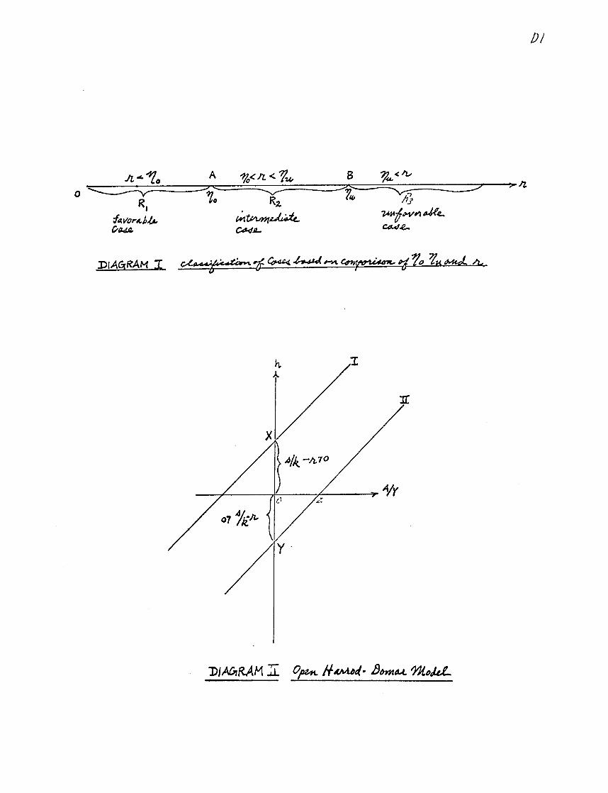
Let us indicate the value of 110 and the value of 1ju by points A and B
on the horizontal axis r representing the population growth rate (see
Diagram I) The two points A and B divide the horizontal axis into three
1 For justification of these choices of names see equation (Al13) in the Appendix
-6shy
regions RI R2 and R3 depending on the comparntive magnitude of the actual
value of r relative to i and a The received doctrine of high populationo
pressure as a barrier to growth is intuitively apparent in this analysis
hence we shall refer to the three cases as
l7a) R (favorable case) o lt r lt 1 implying I lt m
b) R2 iI r lt ijimplying m lt (intermediate case) o lt o
c) R3 (unfavorable case) I1lt r implying o lt m lt 1
We accept the familiar indicators cf success and failure to
evaluate these cased per capita GNP Y per capita coiLsumIptlon C and
per capita savings S We shall say that an economys growth performance
is successful if all these magnitudes increase in the long run Conversely
we construe failure to occur if these magnitudes decrease in the long-run
In Case Rl the favorable case the Harrod-Domar model would lead
us to conclude successful development could be achieved since the population
growth rate r is less than the growth rate of GNP IVand capital 1K Conversely in case R2 the intermediate case and Case R3 the unfavorable
case the Harrod-Domar model would predict failure since the rate of
population growth r exceeds the rate of growth of GNP I and capital 1K
An interesting question arises can a count-y where failure is
predicted by the Harrod-Domar model achieve success by practising austerity
Is it possible to reverse the predicted failure by adopting a high PPSR even
though the average propensity to save is initially low Intuitively if a
country devotes nearly all of its increments in per capita GNP to finance
investment (dissipating little on consumption) one would epect that per
capita GNP and consumption would eventually increase (even though initially
declining) Yet we reach the surprising conclusion that this is not the
case in the closed economy in fact we may state the following theorem
1) In Case R1 the favorable case Y S C and K monotonically
increase from the very beginning of the process Furthermore
the rate of increase of per capita GNP livL4also monotonically
increases
2) In Cases R2 and R3 the intermediate and unfavorable cases Y
St and C monotonically decrease moreover capital stock K
will become negative after a finite time span because
disinvestment will occur
-7-
These conclusions can readily be verified by the following equations describing the time path of the various indicators mentioned in the above theorem (see Appendix)
18a) Y = YP = [akP(o)Ie( u - r)t + a2kP(o) (per capita GNP)
b C = CP = [a(1 - u)kP(o)le(1U - r)t + v2(l-kr)kP(o) (per capita consumption)
c) S = Y - S (per cepita saving)
r)tr) e(iu shy(jIu shym - + e( i - r)t (rate of growth of per
capita GNP)
e) K(t) ale ut + 2efrt (capital stock)
where
19a) Q- = kY (o)m
=b) a2 m - l)kY(o)m
Part i of the above theorem does not cause surprise since the Harrod-Domar model predicts success even where u (the per capita marginal savings ratio) equals s(o) and s remains constant over time However ifu is greater than s(o) the average propensity to save will be increasing through time (l4b) making success even iore obvious In fact it can be shown (see Appendi) that the higher the value of u the higher will be the rate of growth of per capita GNP (l8d) ie
110 gt o for the favorable case
confirming our intuitive notion that greater domestic austerity promotes more rapid growth
Part 2 of the theorem emphasizes the futility of a domestic austerity program i1L an economy where high population pressure exists in combination with a low initial average propensity to save One might even go so far as to depict this as a futile domestic ausLrity situation Failure will always occur regardless of stringent programis to rciae the PiASR For
- 8 shy
such an economy our analysis points to the policy conclusion that in a closed economy population control is the only escape
The economic eplanation of this strong and intuitively paradoxical conclusion is apparent when we realize that per capita GNP is not increasing from the outset because of population pressure Hence the critical austerity variable PIISR has no positive force because there are no positive GNP increments from which per capita saving increments may be mobilized A high PIISR yields additional savings therefore only where per capita GNUp in fact rises
For a country in this situation -- where high population pressure precludes success from even extreme domestic sacrifice -- foreign aid is seen to be strategic in sparking the growth process This external push is indispensable to prod the economy into yielding initial increases in per capita GNP so that domestic austerity -- the high PNSR -- can be made to yield its potential contributions to a cumulative process of raising domestic savings investment and per capita GNP It is this problem on which we focus in the next section
II DOMESTIC SAVINGS VERSUS FOREIGN ASSISTANCE THE OPEN ECONOY A The Harrod-Domar Model
We begin our investigation of combining foreign assistance with domestic savings by exploring the conclusions which can be derived from the familiar Harrod-Domar model We introduce the possibility of adding foreign resources to finance investment I by distinguishing between two sources of finance domestic savings (S)and foreign savings (A)I
Combined with the other basic assumptions the Harrod-Domar Open Economy Model can be described by the following system of equations
j Harrod extends his analysis to an open economy in his equation GC shy s - bwhere G is the grcwth rate (the increment of total production in anyunit period expressed as a fraction of total production) C is theincrease in capital divided by the increment in output (the capitaloutput ratid) s is the fraction of income saved and b is the balance of trade expressed as a fraction of income This formulation howeveris applied only to analyze the impact of the foreign balance on aggregate demand R F Harrod Towards A Dynamic Economics London 1952 Chapter 4
-9shy
2a) I S + A
b) Y- Kk 11c) K IK
d) - r
e) S= sY
We now turn to a problem that will concern us throughout the
remainder of our analysis Let a target rate of growth of per capita GNP h
be given ie
- (ie Y - Y(o)eht)22 1 h
Our investigation will center upon the flow of foreign savings (A)through
time that will be required to advance and sustain such a target We may
think of the target as a politically established goal deemed necessary by
the political leadership as indeed we find in most underdeveloped countries
Alternatively one could consider the adoption of such a target to be the
rate of growth of per capita income that appears to be feasible on the basis
of such considerations as absorptive capacity and the existence of certain
obstacles to growth
From the above assumptions we see that the rate of growth of the
gross national product is
23a) Ij = - 4 + lip - 17p + k h + r (see 22 and 2ld)
b) Y Y(o)e(h + r)t
Since the capital output ratio (k)is constant (2lb) implies that
capital stock must grow at the same rate as Y and hence we have
24 11K = h + r
which may be interpreted as stating that the needed rate of growth of capital
and the demand for investment finance is determined by the population
growth rate (r)and the target growth rate of per capita income (h)
Substituting (24) (2la) and (2lb) in (21c) we have
25 k(h + r) = SY + AY
which states that the demand for investment finance (investment requirements)
I Rosenstein-Rodan embraces the latter concept of the target rate of growth International Aid loc cit pp 111-113
- 10 shy
must be met either from savings supplied internally S or externally from
foreign savings A Notice that the first term on the right-hand side is the
average propensity to save while the second term will be referred to as the
aid-income ratio
It is apparent that equation 25 is generally valid in the sense of
being independent of any domestic saving behavior hypothesis For the Harrod-
Domar savings assumption (2le) this equation reduces to the following
special case
26 h = (s - rk)k + (AY)k
To investigate the relationship between the target rate of growth
of per capita GNP b and the aid-income ratio AY let us represent h on
the vertical axis and AY on the horizontal axis in Diagram II For fired
values of s r and k equation (26) is shown as a straight line with a slope
1k and with a vertical intercept sk - r This diagram demonstrates that
as a country raises its target rate of growth of per capita GNP h (moving
upward on the vertical axis) a higher aid-income ratio AY will be
required Conversely as more foreign savings (a higher aid-income ratio)
become available a higher target h can be sustained
There are essentially two types of dynamic behavior in this open
model as represented by the parallel lines I and II in Diagram II The two
cases are differentiated by the fact that line I has a positive vertical
intercept and line II has a negative vertical intercept
27a) sk gt r Favorable Case (line I)
b) sik lt r Unfavorable Case (line II)
The favorable case is characterized by low population pressure and
(27a) indicates that per capita GNP will increase (at the rate shown as the
vertical distance OX) in the absence of foreign savings If a target higher
(lower) than OX is specified the country will import (export) capital
forever
Conversely in the unfavorable case where population pressure is
great per capita GNP will decrease by OY in the absence of foreign savings
The horizontal distance OZ is the aid-income ratio which would yield
- 11 shy
stationary per capita GNP (h = o) If the aid-income ratio is greater than
(less than) OZ per capita GNP will rise (fall)
Two important conclusions from this application of the Harrod-
Domar model require emphasis First if a country needs a given aid-income
ratio to sustain a specified target h it will require this level of foreigin
savings in Reretuum Assuming that foreign aid is a major component of
foreign savings we see that the very logic of the Harrod-Domar model
precludes a realistic analysis of the problem of a termination date for
foreign aid Our formulation below fills this major gap in existing theory
Secondly when a certain aid-income ratio is required to achieve a given
target h the absolute volume of foreign aid will grow exponentially at the
rate h + r We consider these to be rather unrealistic features Yet the
Harrod-Domar model has provided us with a framework for analysis which we
now proceed to build upon
B The PMVSROpen Economv Model
To recapitulate our argument in Section I our only revision - albeit
a critical one - of the Harrod-Domar model is to replace the savings behavior
assumption (2le) with our assumption based on PMSR presented in (12)
We believe that the model we develop on this basis constitutes an important
step toward realism in planning the finance of economic development We
demonstrate that our method allows both parties in the aid relationship to
analyze in precise terms the growth of domestic saving capacity and hence
foreign savings requirements for reaching self-sufficiency in the developing
country
The savings behavior hypotheses based on PMSR (12) lead to an
average propensity to save given by (l4b) hence the availability of
domestic savings becomes
s - u u -hs(O)28) e ht
if the target rate of growth of per capita GNP is given by (22) When
(28) is substituted in (25) the needed aid-income ratio AY can be
determined residually as
- [u - h()29) AY - k(h + r)
e
- 12 -
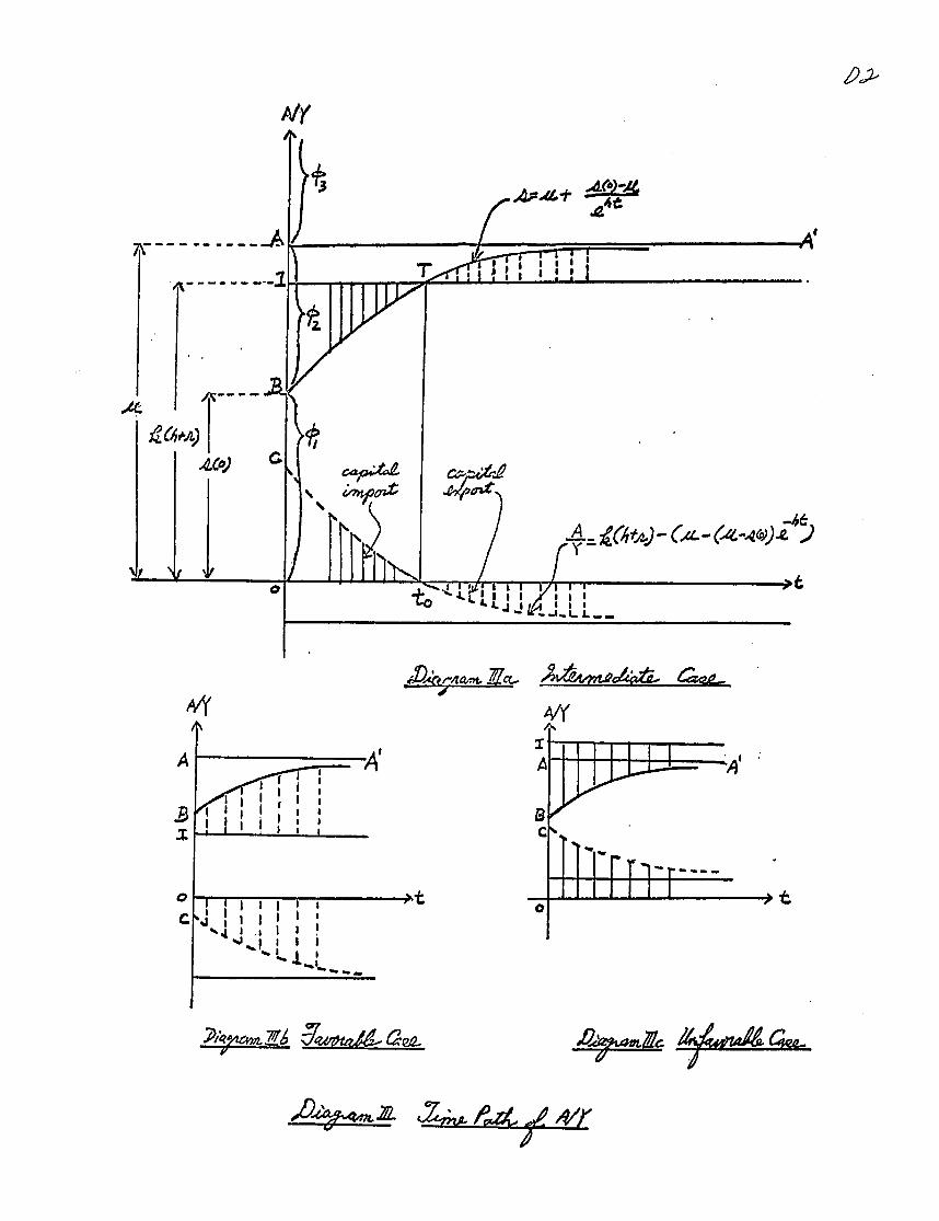
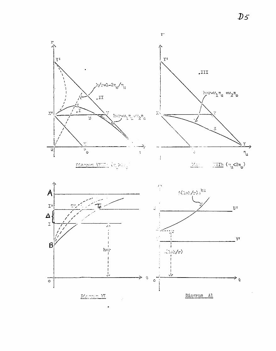
In Diagram ila let time be measured on the horizontal axis and
let the aid-income ratio be measured on the vertical axis in order to plot
the time path of the aid-income ratio AY The following steps are needed
to interpret the diagram
a) Let point I on the vertical axis denote the constant value
of k(h + r) ie total investment requirements
b) Let the time path of the average propensity to save s in
(28) be represented by the positively sloped curve
starting from point B on the vertical axis Notice the
value indicated at point B is the initial average propensity
to save s(o) and that this curve increases monotonically
approaching asymtotically a horizontal line A A where
point A denotes the value of the PMSR ie u This curve
shows that when per capita GNP is growing at a constant
rate h the value of th average propensity to save rises
from its initial value to approach the value of u the P1ISR
c) Let a horizontal line through point I be drawn to intersect
the average propensity to save curve at point T
d) The value of AY will then be represented by the shaded
distance between the two curves or the negatively-sloped
curve starting from point C on the vertical axis
Notice points A and B divide the vertical axis into three regions
T1 2 and b in which point I may fall Making use of the concepts
o -i s(o)k initial growth rate of capital and i = uk long-run growth
rate of capital as defined in (l5a b) of the previous section the three
regions may be precisely defined as
210a) l (favorable case) h + r lt s(o)k -P 1l0
b) 2 (intermediate case) nolt h + r lt uk Ju
c) 3 (unfavorable case) Iju lt h + r
The dynamic behavior of AY the aid-income ratio for the three
cases is represented in Diagrams lia IlIb and lc The favorable case
21 Diagram IIb represents a combination of a low population growth rate r
- 13 shy
and an unambitious target h yielding a situation where no foreign savings
are required in fact the contry will export capital from the outset
Capital exports will constitute an increasing fraction of gross national
product as AY approaches a constant value in the long-run
In the intermediate case 2 shown in Diagram IlIla the country
will need foreign savings at first but there will be a finite termination
date shown by point T (or to on the time axis) After this point has been
reached the country will be able to export capital and to repay whatever
loans were contracted during the period foreign savings were imported
In the unfavorable case 3 shown in Diagram IlIc we see that
foreign savings will be required indefinitely because of a combination of a
high target h and a high population growth rate r The aid-income ratio
AY will eventually approach a constant value implying that the absolute
volume of foreign savings required will grow at a constant rate ie the
rate of growth of gross national product h + r
Before proceeding with further analysis we digress to ecamine the
policy implications in terms of the three cases Obviously Case l the
favorable case need not concern us since domestic savings are adequate to
finance domestic investment requirements to maintain the targeted growth
rate and even to provide a surplus for capital export from the outset Hence
there is no problem of combining foreign and domestic savings indeed with
rare exceptions (eg Nalaysia) we do not envisage underdeveloped countries
falling into this case
The distinction between Case 2 and Case 3 has important policy
significance In the intermediate Case 2 there is a definite termination
date for foreign savings and beyond this date adequate savings will be
generated domestically to provide for loan repayment (in addition to meeting
domestic investment requirements) In other words foreign aid for a finite
period promotes self-help by stimulating progress to the point where selfshy
financed growth becomes possible and the capacity to repay foreign debt
incurred in the process of reaching this point will accelerate Foreign aid
supplied in this situation may be thought of as gap-filling aid since it
allows the country to move toward financial self-sufficiency if the gap
between investment requirements and domestic savings is actually filled during
- 14 shy
the crucial transition period
The unfavorable case 93 does not share these properties Even
though te gap is filled by foreign savings there will be no progress toward
a termination date toward achieving loan repayment capacity or even toward
reducing the rate of flow of foreign savings Our analysis suggests that a
country will remain in this unfavorable situation unless it can reverse the
condition qu lt (h + r) into (h + r) lt 1u-If the initial conditions match
those of Case 3 therefore the strategy appropriate to the interests of
both parties in an aid relationship should be aimed at moving the country
to a more favorable situation The basic operational principle of the
strategy would consist of the recipient country adopting domestic policy
measures to narrow the gap sufficiently to produce a reasonable termination
date Hence we refer to this as the gap-naKrowin aid case
We note that our approach in this section leads toward a more
meaningful interpretation of self-help We define self-help as a foreign
assistance-stimulated program of domestic austerity to generate an adequate
supply of domestic financial resources over time to ensure reasonable and
finite dimensions to the foreign assistance program The distinction between
gap-filling and gap-narrowing foreign aid prcqides a realistic basis for
applying the self-help criterion In the case of countries qualifying for
gap-filling aid an adequate flow of foreign savings will enable the economy
to progress toward self-sufficiency in development finance merely as a
result of adequate capital assistance In other words foreign aid of this
type may be viewed as automatically assisting the countrys austerity
program to fulfill the self-help condition without careful administrative
supervision This is tantamount to finding adequate absorptive capacity
in the sense that gap-filling aid is absorbed to enhance the capabilities
l Note that in the closed economy analysis in the first section the
crucial condition for success is r lt io ie the population growth rate must be less than the initial growth rate of capital while in this open economy case the crucial condition for a finite termination date is (h + r) lt u ie comparison between h + r and the long-run growth of capital
Policies appropriate to this strategy are discussed in Section IV
- 15 shy
of the recipient country to generate a sustained and cumulative growth process from domestic resources- This type of absorptive capacity does not exist in the other case 3 where foreign aid fails to automatically contribute to improvement of domestic financial capabilities
In this latter case therefore the more demanding assistance task of narrowing the gap between growth requirements and domestic financial capacity is implied if the self-help criterion is to be met Capital assistance alone will merely plug a long-run gap and permit a country to live beyond its means - without generating leverage effects toward greater self-help The policy conclusion is that foreign aid of a package-deal type is required in this case conditions for progress toward greater self-help must be analyzed and specified The recipient country should be induced to accept a firm commitment to narrow the gap so that foreign aid will begin to spark the growth of domestic savings capacity If a program of foreign assistance cannot be devised to satisfy the self-help criterion by narrowing the gap in such countries there are strong economic grounds for withholding assistance- The task of providing gap-narrowing aid therefore requires a more flexible and imaginative approach than in the gap-filling case Here the art of providing useful assistance requires sophistication and diplomacy and costs and administrative demands are likely to be high It follows that foreign technical assistance has a special role here since we would envisage a need for expert external advice in assisting the country to devise and implement domestic policy measures for changing tbe adverse initial conditions
1 We note that Professor Rosenstein-Rodan also uses this condition as oneof several interpretations of absorptive capacity See P N Rosenstein-Rodan Determining the Need for and Planning the Use of External ResourcesOrganization Planning and Programming for Economic Development ScienceTechnology and Development United States Papers Prepared for the UnitedNations Conference on the Application of Science and Technology for theBenefit of the Less Develop ed Areas Vol VIII pp 70-71
2 We wish to emphasize however that political and security considerationsfall outside this analysis and that in the real world non-economic criteria may turn out to be of overriding importance
- 16 -
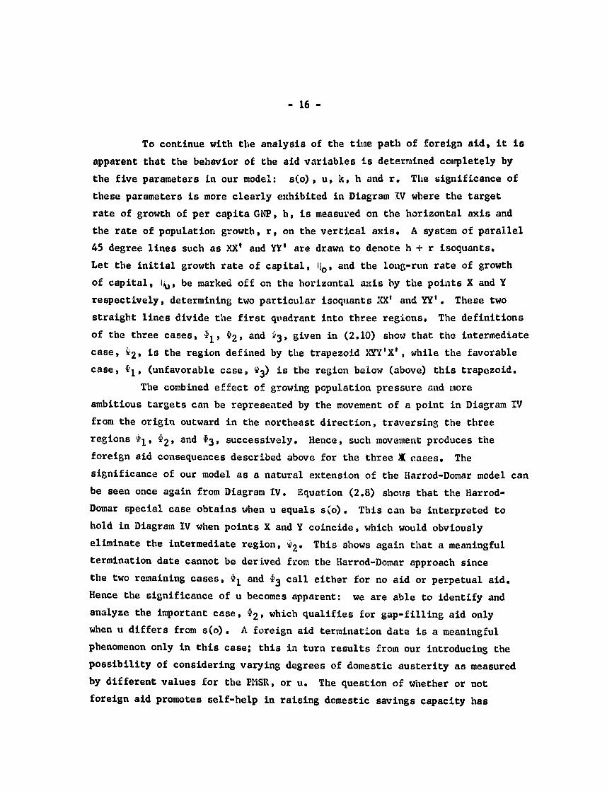
To continue with the analysis of the time path of foreign aid it is
apparent that the behavior of the aid variables is determined completely by
the five parameters in our model s(o) u k h and r The significance of
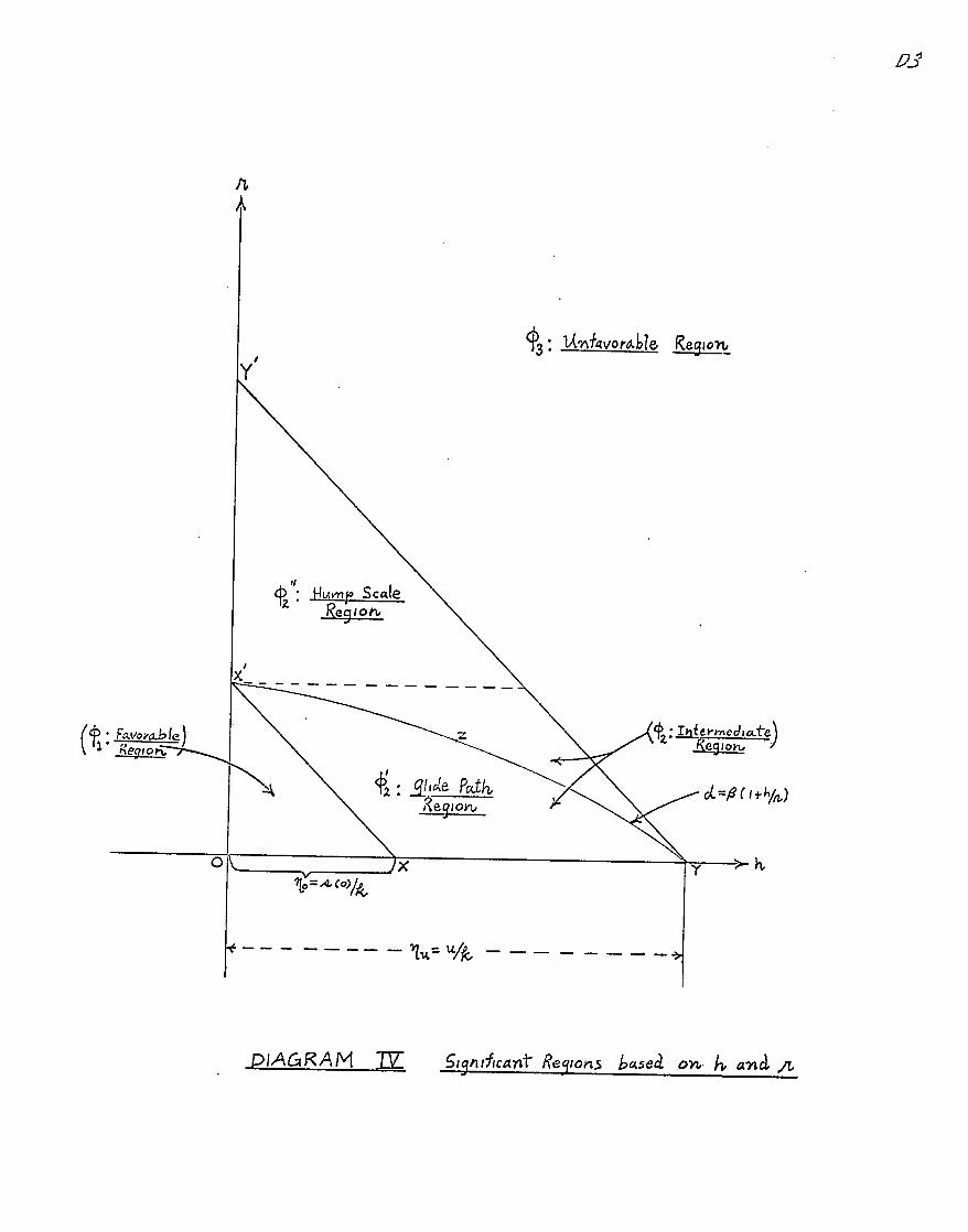
these parameters is more clearly exhibited in Diagram IV where the target
rate of growth of per capita GNP h is measured on the horizontal axis and
the rate of population growth r on the vertical axis A system of parallel
45 degree lines such as XX and YY are drawn to denote h + r isoquants
Let the initial growth rate of capital Io and the long-run rate of growth
of capital li be marked off on the horizontal atis by the points X and Y
respectively determining two particular isoquants XX and YY These two
straight lines divide the first quadrant into three regions The definitions
of the three cases l 2 and 3 given in (210) show that the intermediate
case 2 is the region defined by the trapezoid XYYX while the favorable
case 1 (unfavorable case 13) is the region below (above) this trapezoid
The combined effect of growing population pressure and more
ambitious targets can be represented by the movement of a point in Diagram IV
from the origin outward in the northeast direction traversing the three
regions D1 t2 and b successively Hence such movement produces the
foreign aid consequences described above for the three X cases The
significance of our model as a natural extension of the Harrod-Domar model can
be seen once again from Diagram IV Equation (28) shows that the Harrod-
Domar special case obtains when u equals s(o) This can be interpreted to
hold in Diagram IV when points X and Y coincide which would obviously
eliminate the intermediate region 2 This shows again that a meaningful
termination date cannot be derived from the Harrod-Domar approach since
the two remaining cases I and b call either for no aid or perpetual aid
Hence the significance of u becomes apparent we are able to identify and
analyze the important case 2 which qualifies for gap-filling aid only
when u differs from s(o) A foreign aid termination date is a meaningful
phenomenon only in this case this in turn results from our introducing the
possibility of considering varying degrees of domestic austerity as measured
by different values for the PMSR or u The question of whether or not
foreign aid promotes self-help in raising domestic savings capacity has
- 17 shy
special importance We see now that there is a positive relationship
between the two in only one of the three regionLs the one adurmbrated by
traditional analysis of the Harrod-Domar type
In addition to the termination date dimension of the problem it
is important for both aid-giving and aid-receiving countries to plan in
advance the volume of aid requirements and how it is likely to change over
time More deliberate evaluation of long-run commitments and obligations
become possible with such knowledge and the danger of mere year-to-year
improvised programs is reduced If applied such knowledge could make for
a more rational use of foreign aid by reducing uncertainties for both parties
For discussion of this problem we return to Diagram IV We
already know that in region I no foreign aid is needed and in region 3
foreign aid will increase monotonically Concentrating on the intermediate
case 2 therefore we derive the volume of foreign aid through time as
A = [k(h + r) - (u - (u - s(o)e ht)]Y by (29)
= [k(h + r) - u + (u - s(o)e-ht y(o)e(h + r)t oby (23b)
(lh + r - uk + (uk - z(o)k)eht]IK(o)e(h + r)t by (21b) and hence
21la) A = K(o)e(h + r)t (e-ht 0) where
o= =b) a Iu1- uk - s(o)k
c) P 16 i= uk- (h+ r)
To see the direction of change in A it will be shown in the
Appendix that the region 2 has two subregions 2 and D2 divided by a
boundary curve XZY in Diagram IV given by the following equation2
212) t = f(l + hr)
when at and 5 are defined in (21lbc) In other words the
two subregions are defined by
I Heuristically since a is the difference between the long-run growth rate of capital and the initial growth rate of capital it may be termed the potential difference in capital growth rates Given k and s(o) the magitude of this potential difference is directly related to the national austerity index as measured by u (PMSR)
2 It will be shown in the Appendix that the boundary line passes through the points X and Y The exact shape of the boundary line and its economic significance will be discussed in the next section
- 18 shy
213a) 2 (glide path case) a lt 3(l + hr)
b) 2 (hump-scaling case) P(1 + hr) lt a
Although there is a finite termination date for both sub-regions
there is a difference in the shape of the time-path of the volume of foreign
2 the volume of aid first rises to a maximum andaid A In sub-region
The aid volume conclusions therefore can be distinguishedthen decreases
more picturesquely as a egt case for the sub-region 2 and a humpshy
scalinR case for 2 In the glide-path case the process of growth of
domestic savings capacity operates to continuously reduce foreign aid
requirements and external assistance may be viewed as gliding down a path
progressively nearer self-sufficiency No particular aid counsel is needed
here since the end of the task is in sight and the burden of assistance
continuously declines Both conditions are attractive to countries providing
assistance
In the hump-scaling case on the other hand although the
termination of aid is a known prospect the peculiar behavior of the needed
volume of aid may raise doubts from the aid-giving countrys viewpoint
The hump of a maximum volume of assistance must be scaled before a glideshy
path phase to ultimate success appears This analysis therefore has
special value for distinguishing among countries where an increasing annual
volume of assistance is required With the assurance that a country falls
into sub-region the fear of an ever-growing volume of assistance that
will never terminate may be allayed In this special case we counsel patience
This incidentally justifies a big initial push approach to foreign assistshy
ance for countries where austerity programs exist but where the hard road
to self-sustained growth involves growing foreign aid before the self-help
response begins to reduce the required volume
III QUANTITATIVE ASPECTS OF PLANNING FOR DEVELOPMENT ASSISTANCE
As the analysis has proceeded we have pointed to implications for
improving the principles of development assistance strategy applicable to
both aid-giving and aid-receiving countries In the previous sections the
underlying theory was mainly based on qualitative analysis in this section
= 19 shy
a more quantitative basis is supplied This amplification leads to further
clarification of the self-help concept and it also provides methods for anshy
alyzing alternative time and volume patterns of foreign assistance
Solutions to the quantitative problems raised in this section therefore
are essential for strengthening the theoretical basis underlying development
assistance policy (which we consider in Sections IV and V) as well as for
the statistical implementation of our model
A Quantitative Analysis of Termination Date
We have consistently stressed the Importance of the planned
termination date for foreign assistance Analysis of the intermediate case
2 in the previous section provided a basis for relating termination date to the self-help criterion and for giving concrete meaning to self-help as
a measure of country performance We recall that termination date estimation
is relevant only for this case In the favorable case I no foreign
assistance is needed while in the unfavorable case 3 foreign assistance
will never terminate The termination date can be determined by setting the
aid-income ratio (AY) in 29 equal to zero
n- u-3 1 j s(o) -l I In [u k(h + r) ]31 to h- l - - h ln ( )
where i= uk - s(o)k and j - uk - (h+ r) as defined above in (21lbc)
We know that aO gt I for the intermediate case hence a positive termination
date to can always be found
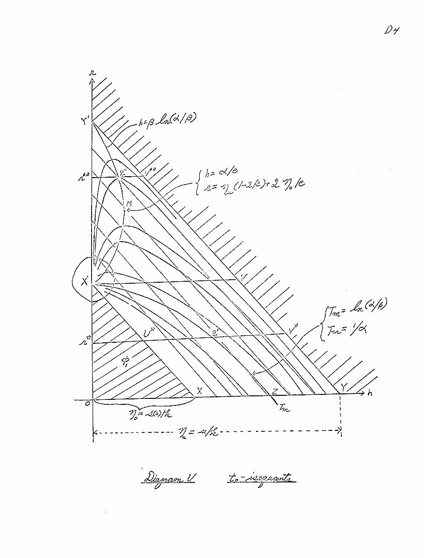
Diagram V is a reproduction of Diagram IV in the previous section
In the trapezoid XYYX which represents the intermediate case Y2 we draw
parallel h + r isoquants and also a system of to (termination date) isoquants
the latter determined from equation 31 This equation indicates that
upward movement along any specific h + r isoquant will increase the termination
date to since ln(cy0) remains unchanged and h decreases Geometrically this
can be seen from the fact that upward movement along an h + r isoquant cuts
successively higher termination date (to) isoquants This implies that the
slope of the to isoquant is greater than -1 Economic meaning can be given
to this fact by first noting that the slope of the to isoquant may be thought
of as a marginal rate of substitution between h and r leaving the termination
- 20 shy
date unchanged The fact that the marginal rate of substitution is greater
than -1 means that a reduction in the target rate of growth of per capita GNP
h of 5 per cent for example will fail to compensate for the termination
date lengthening effect of a 5 per cent increase in the rate of population
growth r Hence the numerical rate of population growth exerts greater
weight on the termination date than the per capita GNP growth target
This phenomenon may be explained by use of an additional diagram
In Diagram VI let Diagram lia be reproduced The time path of the average
propensity to save is given by the solid curve Bs and the horizontal line
beginning from I (determined by h + r) intersects Bs at point T the
termination date Supposing r increases by the value of A the termination
date is seen to be lengthened to the point To o Conversely if the value of
h is increased by A (raising point I to I) the termination date is raised
only to the point T since an increased value of h will according to equation
28 also raise the Bs curve (the average propensity to save) to the position
of the dotted Bs curve
The map of to isoquants which is defined in the trapeziid XYYX in
Diagram V has a number of important properties that will be useful to our
analysis These properties are rigorously deduced in the Appendix while it
suffices here to state them and to investigate their economic meaning
(P1) The boundary between regions i and 2 ie line XX may be construed
to be the first to isoguant with a zero termination date
Notice that along this boundary line h + r = o - s(o)ki- As we have
seen in terms of Diagram lIla this means that point I coincides with point B From this diagrammatic analysis it is apparent that in this boundary
situation a country will be self-supporting in investment finance
at the outset and that it will begin exporting capital in the second year
The first rise in the average propensity to save as it is pulled upward by the force of the PNSR operating through the initial increase in per capita GNP
provides a surplus of domestic savings over investment requirements
(P2) The boundary between regions 2 and 3 line YY may becqnstrued to be
the last to isouant Les the to joguant with an infinite termination date In Diagram Mliathis corresponds to the situation where point I
coincides with point A and foreign savings would be required forever Even
- 21 shy
when the full force of the PMSR becomes effective and the average propensity
to save approaches the PMSR domestic savings will be inadequate to finance
the high investment requirements (P3) The left-boundary of relin 2 line XY maybe construed to be an
extension of the infinite termination date isoquant definedin P2
According to P2 and P3 the entire isoquant with the infinite terminashy
tion date is the broken line XYY The economic significance of the segment
XY can be seen from the fact that it coincides with the vertical axis and
hence the target rate of per capita GNP growth h is zero This means that the PMSR is impotent Thus equation 28 is reduced to s - s(o) the Harrod-
Domar case where a constant average propensity to save continues through
time In the terms of reference in Diagram lia this situation would show the
average propensity to save through time as a straight horizontal line beginning
from point B rather than as an increasing curie Point I would lie above
point B and the vertical distance from horizontal parallel lines beginning
from I and B would show that foreign savings would be required for all time
(P4) The bottom boundary of region 2 line XY is a line along which
successive increases in the target h from X to Y will cut to isoguants
increasing from 0 at X to infinity at Y
This is the special case in which the rate of population growth r
is 0 ie population is stationary In terms of Diagram IlIla the height
of point I would be simply kh rather than k(h + r) As I rises from point B
to point A the termination date indicated by point T increases from zero
to infinity
(P5) All to isoguants begin from point X
This point X represents the special conditions h - o and r - s(o)k
which may be interpreted as the simplest Harrod-Domar case involving stable
per capita GNP with neither foreign savings nor capital export Domestic
savings are just adequate to maintain the constant rate of population growth
at a constant per capita GNP level a situation which might be described as a
self-sufficient stationary state
Diagram V may now be used to elucidate further several types of foreign
assistance situations in terms of termination dates We concentrate first
on cases falling in the vicinity of X marked off in the diagram by a small
- 22 shy
circle Countries within this circle are in a precarious situation Small
variations in the value of any important parameter will open the whole range
of possible foreign aid termination results A small favorable change - or
positive stimulus - within the system (such as a slight increase in the initial
savings rate s(o)p reduction of the population growth rate r or lowering
the capital-output ratio k) will reverse immediately a perpetual capital
import situation to one in which capital export will continue forever On the
other hand a slight unfavorable change - or negative shock - will lead to the
postponement of the termination date possibly to infinity even though the
country had previously been exporting capital It is difficult to specify
desirable foreign assistance policy relevant to this small circle beyond the
caveat that wariness is necessary Countries in this category show low or even
negative per capita GNP targets hardly consistent with development assistance
goals or the criterion of self-help since we know that the PRSR will be either
impotent or negative M1oreover the situation is highly volatile small variashy
tions in parameter values will produce drastic changes in aid requirements shy
as seen from the wide diversity of termination date possibilities Given the
present hazardous state of statistical information about underdeveloped
countries an attempt to apply our quantitative criteria here would run the
risk of large margins of error in projecting the foreign aid magnitudes
The target rate of growth h itself turns out to be a critical
variable for determining termination dates for foreign assistance While we
would normally expect a more ambitious target to lead to a postponement of
termination date it may come as a surprise to learn that for many realistic produce
cases a higher target will in fact pvee a shorter termination date
To introduce this unexpected result of our analysis the following property
of the to isoquant system in Diagram V may be stated
(P6) There is a critical value for a specific termination date isoauant
Tm such that all to isoguants__) are eatvely sloped for to lt Tm and
(b) reach a maximum point for Tm lt to
From properties PI P4 and P5 above it is apparent that the system of
to isoquants will begin from X with negatively sloped curves for small values
of to near XX However properties P2 and P3 imply that as the value of to
increases the isaquants will gradually shift upward approaching the shape
of the broken line Wwhen to becomes sufficiently large Hence there isX Y
- 23 shy
a critical termination date Tm associated with a specific isoquant that provides a boundary between a class of negatively sloping isoquants and a class of inverted U-shaped isoquants It is shown in the Appendix that the
value of Tm (the critical termination date or CTD) and hence the isoquant
corresponding to Tm (CTD isoquant) are
32a) Tm =Ia = Iil- 0 (critical termination date or CTD)
b) 1a = hr (aO)n (CTD-isoquant)
where a is as defined in 211b
Hence the value of Tm is completely determined by u s(o) and k For example where u - 20 s(o) = 10 and k = 33 Tm 33 years= In Diagram V the isoquant corresponding to Tm is indicated by the curve XZ
Using the above properties P1 to P6 wa can readily plot the contour map of the to isoquants as in Diagram V all isoquants begin at point X1 and terminate at a point on segment XY Higher isoquants indicate longer terminashytion dates from zero to infinity The isoquant XZZ is a boundary line dividing the contour lines into two types those below it are negatively
sloped and those above it have a maximum point With this characteristic of the to isoquant system in mind we can extend the analysis by drawing an auxiliary horizontal line XV through the point X in Diagram V This line
divides the 2 region into two sub-regions an upper triangle XVY and a lower parallelogram XXYV We refer to the first sub-region as the triangular region and any point belonging to it as a triangular case The
second sub-region is termed the parallelogram region and it contains
parallelogram cases It is now apparent that these situations are distinguished by the fact that in the parallelogram the termination date contour lines
decrease continuously while in the triangle all to contour lines lie above
the boundary isoquant XZZ and have a maximum point It is shown in the Appendix that the locus of the maximum points for to isoquants in the trishy
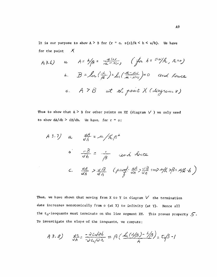
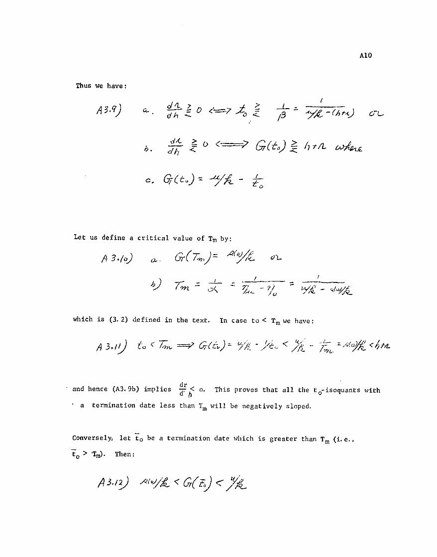
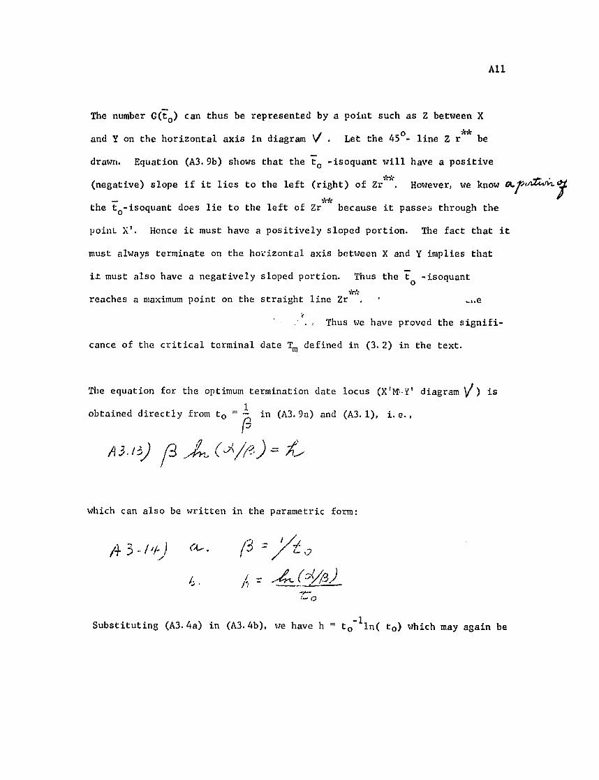
angular region is given by the equaticn
33 P in() = h
With u k and s(o) specified equation 33 determines a curve XMY in Diagram V which heuristically may be referred to as the optimum target locus Point M denotes the maximum value of h on the optimum target locus
- 24 shy
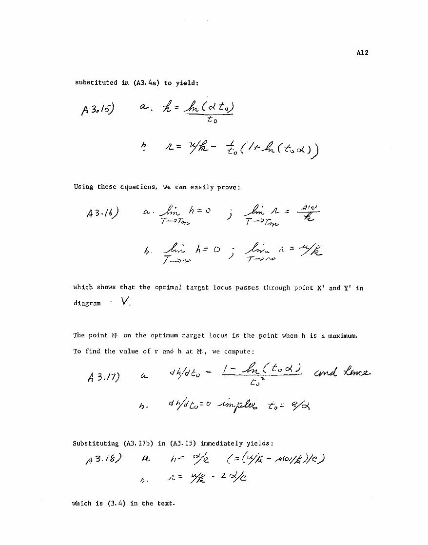
the coordinates of Mgiven by
34a) h - ae
b) r- 16- 2h - -W2e
where e (- 271828) is the basis of the natutal logarithm We
now proceed to analyze the economic significance of the two regions beginning
with the parallelogram XXYV
i The Parallelogram Region
The implications of the more straightforward parallelogram cases
follow from the fact that the to isoquants are all negatively sloped As we
would expect an increase in the target h or an increase in the population
growth rate r will increase the termination date to This is seen by the fact that as a point moves to the northeast it will always fall on a higher
to isoquant
Let the horizontal line rv cut across the parallelogram region as inDiagram V Point r represents a case in which the initial average
propensity to save s(o) yields an initial growth rate of capital 10 = s(o)k
which at the Point X exceeds the population growth rate at r It is
immediately apparent that per capita GNP can be raised in a closed economy Even in the context of the Harrod-Domar model inwhich u = o a constant
rate of increase of per capita GNP [equal to the vertical distance rX
(= 11- can be sustained in closed economy However if u gt o (as weo r)] a assume in our model) the economy could not only maintain the same rate of
increase in per capita GNP but it could also export capttal This follows from the effects of a positive PkiSR which would produce additional savings
from the increments in per capita GNP (See discussion of favorable case
portrayed in Diagram IlIb) Indeed such a country could continue to export
capital even though the target b be raised to any value less than rU
If however the target is set at a point such as Z where the value of h
is greater than rU foreign savings will be required for a finite time span to maintain the targeted increase in per capita GNP Eventually the positive
1 More specifically the equality rX - rU implies that the target h at U (ie rU) equals the initial rate of growth of per capita GNP (rX)sustainable in a closed economy even where u equals zero
- 25 -
PMSR operating through rising GNP per capita will cause the average propensity
to save to rise enough to eliminate the foreign aid gap between investment
requirements (h + r) and the growth rate of GNP that can be financed by
domestic savings
The horizontal distance UV (equivalent to a - ju - i1oin 21lb) is
a measure of the extent by which a country can raise its target h beyond
point U under the gap-filling aid coadition This condition it will be
recalled implies the constraint that a finite termination date must be built
into the system Thus with s(o) and k fixed the significance of greater
domestic austerity (ahigher value of u the PMISR) is that it allows a
country to adopt a higher per capita GNP growth ratp target while continuing
to qu1ify for gap-filling aid
The growing political furor over the length of the U S development assistance commitment underlines the need for evaluating the time horizon of
foreign aid with both precision and realism For this reason it is important
to apply our model to the real world -o produce some sense of the order of
magnitude of the termination date for gap-filling aid Let us take a fairly
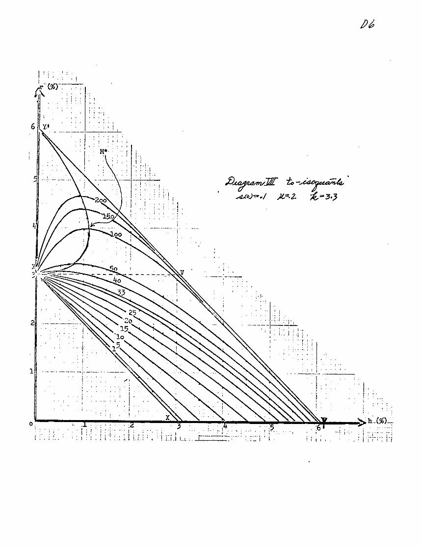
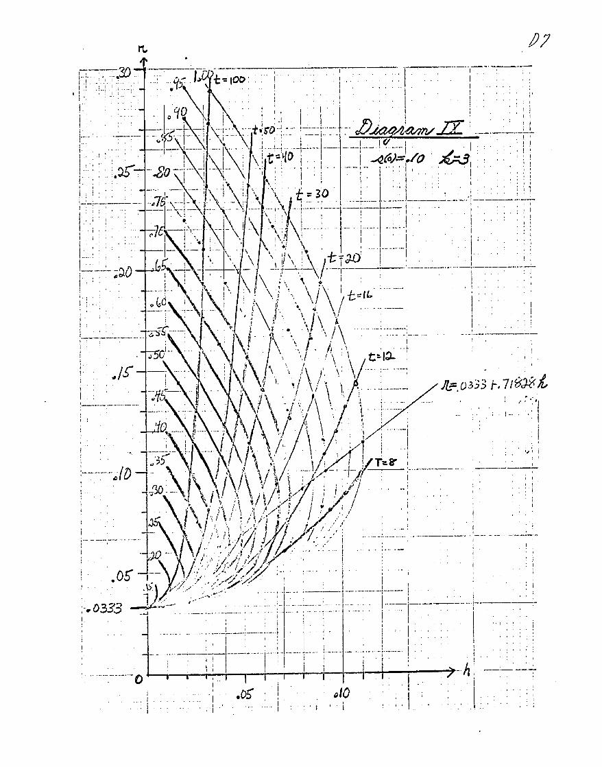
typical situation as an application of our model Diagram VII presents the
termination date isoquants for the case where (i) the initial average
propensity to save s(o) equals 10 (ii) the per capita marginal savings
ratio u equals 20 and (iii) the capital-output ratio k equals 331- The
parallelogram case as in Diagram V is again shown as the region XXYV
Given a population growth rate r of 2 per ceat our typical
country could maintain a targeted rate of growth of per capita GNP h of
1 per cent per year without requiring foreign aid An increase in the target
to 15 per cent per year however would involve foreign aid for about 12-13
years while a target of 2 per cent per year would raise the foreign aid
termination date to 20 years
1 Statistical estimation of these parameters (u s(o) and k) in Table III of this section shows that these values approximate those for several developing countries most closely for Greece Israel and Turkey
- 26 -
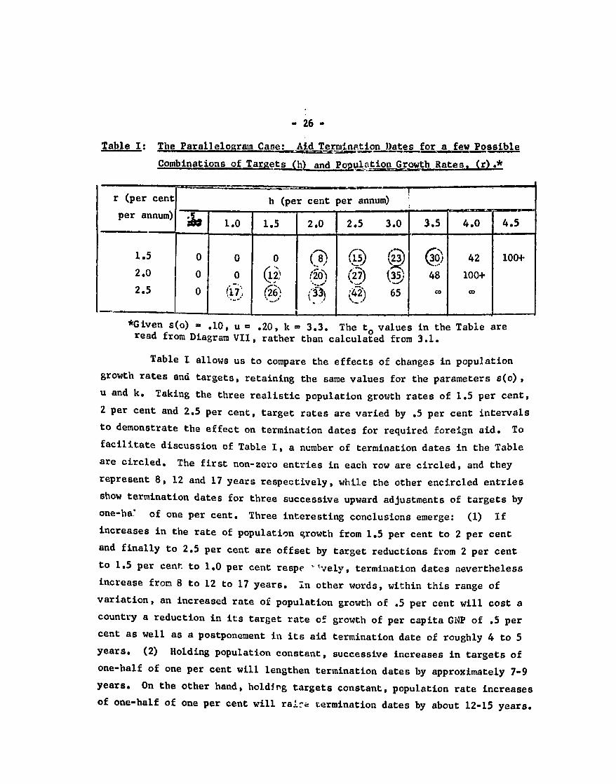
Table I The Parallelogram Case Aid Termination Dates for a few Possible
Combinations of Targets (h andopulition Growth Rates (r)
r (per cent b (per cent per annum)
per annum) 10 2015 25 30 35 40 45
15 0 0 0 D8 (is5) 3~ (3i) 42 100+ 20 0 o (12 74
25 0 (171 f26) it 65
Given s(o) 10 u = 20 33k The to values in the Table are read from Diagram VII rather than calculated from 31
Table I allows us to compare the effects of changes in population growth rates and targets retaining the same values for the parameters s(o) u and k Taking the three realistic population growth rates of 15 per cent 2 per cent and 25 per cent target rates are varied by 5 per cent intervals to demonstrate the effect on termination dates for required foreign aid To facilitate discussion of Table I a number of termination dates in the Table are circled The first non-zero entries in each row are circled and they represent 8 12 and 17 years respectively while the other encircled entries
show termination dates for three successive upward adjustments of targets by one-ha of one per cent Three interesting conclusions emerge (1) If increases in the rate of population growth from 15 per cent to 2 per cent and finally to 25 per cent are offset by target reductions from 2 per cent to 15 per cent to 10 per cent respe vely termination dates nevertheless increase from 8 to 12 to 17 years in other words within this range of
variation an increased rate of population growth of 5 per cent will cost a country a reduction in its target rate of growth of per capita GNP of 5 per cent as well as a postponement in its aid termination date of roughly 4 to 5 years (2) Holding population constant successive increases in targets of one-half of one per cent will lengthen termination dates by approximately 7-9 years On the other hand holding targets constant population rate increases of one-half of one per cent will ralfa termination dates by about 12-15 years
- 27 shy
(3) Increases in the target beyond the circled values will cause drastic
lengthening of the duration of foreign aid or shift the country into the Q3
region where it no longer qualifies for gap-filling aid Even where termination
dates become drastically raised it would be realistic to view the country as
moving into the category where gap-narrowing aid strategy becomes appropriate
From the qualitative analysis in our previous section we defined the gapshy
filling aid case in terms of the existence of a finite termination date We
must take account however of the political climate in aid-giving countries
and the limitations of our capacity to predict the future from imperfect data
These problems make an unduly long termination date difficult to justify In
our judgment therefore there is likely to be a maximum termination date
beyond which the aid-giving country will be induced to adopt the gap-narrowing
strategy Considering the precedent of the short 10-year span of Marshall
Plan aid the vacillation in the conviction withAlonger term aid has subseshy
quently been given and the growing congressional impatience with the failure
to see an end to the present assistance task to underdeveloped countries it
is probably unrealistic to think in terms of aid to any country extending
beyond one generation - roughly 35 years
In the typical case exhibited in Table I all entries to the right of
the circled values represent termination dates which we judge to be politically
unacceptable for gap-filling aid All exceed 35 years and any further rise in
targets by only one-half of one per cent will drastically increase the duration
of foreign assistance Thus given a realistic range of population growth
rates from 15 to 25 per cent targets must be specified within the range
between 15 and 35 per cent to yield politically feasible termination dates
Furthermore our analysis provides a method for precise measurement of the
impact of changes in both targets and population growth rates on termination
dates For example in this reasonable range simultaneous reduction of both
population growth rate and target by one-half of one per cent will reduce the
termination date by about 20 years
ii The Triangular Case
The triangular region is shown in Diagram V as the triangle XVY
A horizontal line rV is drawn to cut across this region intersecting the
optimum target locus at point Z If the population growth rate is given for
- 28 shy
example at r an optimum target will be found equal to the horizontal
distance rZ This target will be associated with Lne minlmum termination
date (ViTD) for foreign aid given the initial conditions Any target of
higher or lower value will produce a termination date exceeding the MTD
This interesting phenomenon can be easily explained We already know
from Property P3 that a country located at r will suffer decreasing per
capita GNP in a closed economy of the Harrod-Domar type (ie where the PMSR
u equals 0) because the initial growth rate of population growth r exceeds 1
the initial growth rate of gross national product 11- It follows that in0
an open economy foreign aid will be needed forever merely to sustain the
initial stationary level of per capita GNP At point r where h - o the
PM4SR has no force in raising the domestic propensity to save since per capita
GNP is constant A positive target (hgt 0) will aeetvite the PMSR up to
point Z the higher the target the greater will be the effect of the PMSR
in raising the average propensity to save and hence in shortening the
termination date Beyond point Z however increases in the target will
begin to postpone the termination date as in the parallelogram region
The rationale behind this phenomenon can be seen from Diagram VI in
which the termination date is indicated by point T where the solid average
propensity to save curve Bs intersects the horizontal investment requirements
curve (IT) determined by h + r Suppose the target is raised by the value of
L shifting the horizontal curve IT to IT the increased target will also
shift the average propensity to save curve Bs upward If the shift in Bs is
relatively large (eg to position Bs) the resulting termination date TV
will be less than the original termination date T If on the other hand
the shift in Bs is relatively small to position Bs the termination date T
will bc larger than the original T
The triangular region it is apparent is less favorable than the
parallelogram region because of high population pressure We would expect
therefore more dismal aid termination date conclusions for this region
Again using the typical parameter values employed for Diagram VII ie
s(o) - 10 u - 20 and k - 33 we present in Table II the minimum termination
dates and the optimum targets for alternative population growth rates
I1 The rate of decrease in per capita GNP will be equal to the distance Xr
- 29 -
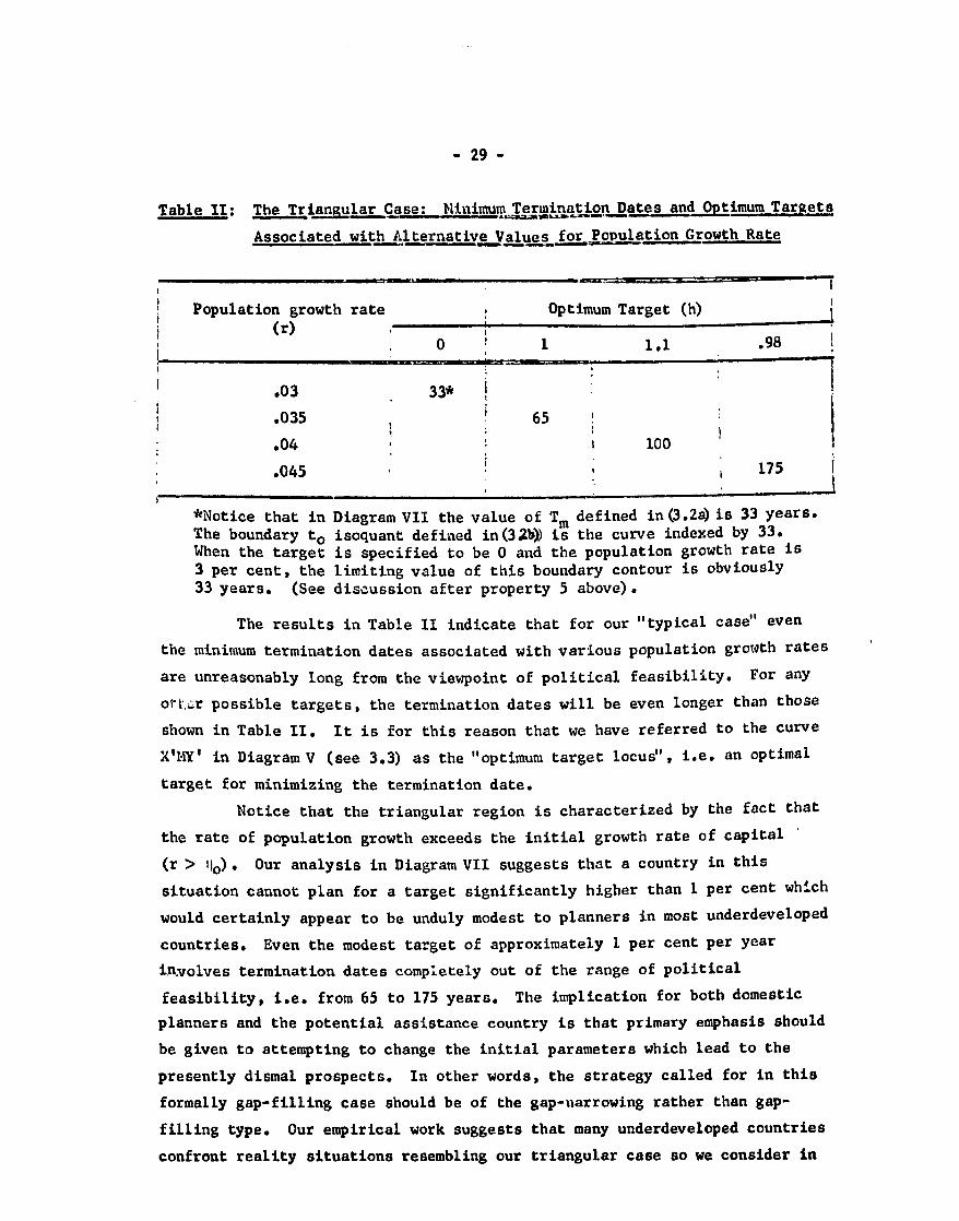
Table II The Trianlar Case Minimum Termination Dates and timum Targets
Associated with Alternative Values f Population Growth Rate
Population growth rate Optimum Target (h) (r) 0 1 11 98
03 33
035 65
04 1 100
175045
Notice that in Diagram VII the value of Tm defined in (32a)is 33 years The boundary to isoquant defined in(3b) is the curve indexed by 33 When the target is specified to be 0 and the population growth rate is 3 per cent the limiting value of this boundary contour is obviously 33 years (See discussion after property 5 above)
The results in Table II indicate that for our typical case even
the minimum termination dates associated with various population growth rates
are unreasonably long from the viewpoint of political feasibility For any
otgr possible targets the termination dates will be even longer than those
shown in Table II It is for this reason that we have referred to the curve
XMY in Diagram V (see 33) as the optimum target locus ie an optimal
target for minimizing the termination date
Notice that the triangular region is characterized by the fact that
the rate of population growth exceeds the initial growth rate of capital
(r gt 11o) Our analysis in Diagram VII suggests that a country in this
situation cannot plan for a target significantly higher than 1 per cent which
would certainly appear to be unduly modest to planners in most underdeveloped
countries Even the modest target of approximately I per cent per year
involves termination dates completely out of the range of political
feasibility ie from 65 to 175 years The implication for both domestic
planners and the potential assistance country is that primary emphasis should
be given to attempting to change the initial parameters which lead to the
presently dismal prospects In other words the strategy called for in this
formally gap-filling case should be of the gap-narrowing rather than gapshy
filling type Our empirical work suggests that many underdeveloped countries
confront reality situations resembling our triangular case so we consider in
- 30 -
Section IV the problem of gap-narrowing strategy in greater detail
B Quantitative Analysis of Ad Flows
In our quantitative analysis above termination date problems have
been singled out for rigorous quantitative investigation This emphasis is
based on our concern about the political diatribe directed at this aspect of
foreign aid in recent congressional consideration of annual aid appropriation
bills1 However this emphasis on the termination date should not obscure the )
fact that there are other important dimensions to planning foreign assistance
It is obvious that problems related to absolute magnitudes of foreign aid
flows through time also deserve explicit investigation Our analysis of these
problems is based on equation 211a which described the time path of foreign
aid flows A(t) Specifically we examine two key planning aspects of A(t)
(1) the date of the peak year of the aid flow and the volume of aid at this
peak year and (2) the accumulated volume of foreign aid over time
i Peak Flow Analysis
Referring to Diagram IV in the previous section we recall that the
trapezoid XXYY (comprising all cases with a finite aid termination date to
and labelled the i2 region) was divided by the boundary line XZY into humpshy
scaling aid cases (XYY) and glide-path aid cases (XXY) In investigating
the precise location of this boundary line we find that it may be of two types
depending on the comparative values of li(-uk) and go(=s(o)k) more
specifically on whether or not iuis more than twice the value of li Thus
the two possibilities are
35a) 21j o lt It
b) 11o lt 1ju lt 2110
Diagrams Villa and VIlIb represent these two possible types of
boundary lines between the hump-scaling and the glide-path aid cases In both
diagrams the intermediate region XLY is divided by the boundary curve XZY
with the hump-scaling case above the curve and the glide-path case below
Diagram Villa corresponds to (35a) and in this situation the boundary curve
XZY penetrates into the triangle XVY and reaches a maximum at point Z It
can be shown that the ratio of hr at point Z satisfies the condition
36 hr - I - 211o1
L An example of such a discussion was held on the Senate floor and was recorded in the Congressional Record Proceedings and Debate of the 88th Congress 1st Session Volume 109 Number 177 November 4 1963 p 19944
- 31 -
Diagram VIIb corresponading to (35b) depicts a situation in which
the boundary curve is negatively sloped and remains within the parallelogram
XXYV The distinction between the two cases shown as Diagrams VIIIa and
VIIIb is based on investigation of the equation of the boundary curve which
can be shown to be
37a) h + r - Wlii + W21o where
b) W a 1 +hrhran and
1c) W2 - 1 + hr
The economic interpretation of this result in terms of the distinction
made for termination date analysis between parallelogram and triangular regions
may be briefly stated In the simpler case w~here u is less than twice the
value of s(o) )iagram VIlIb) the triangular region includes only humpshy
scaling aid cases Conversely where u is greater than twice the value of
s(o)--signifying relatively higher domestic austerity effort--a part of the
triangular region is converted into glide-path aid cases where the conditions
for automatic gap-filling aid are more directly apparent- (See end of
Section It) The implication for the parallelogram region is that glide-path
cases will exist for both boundary types unless the termination date is too
remote since we know from Diagrams V and VII that the shaded areas in Diagrams
Villa and b involve long termination dates Here too we can see the force
of a relatively high u in Diagram Villa where u is relatively high the humpshy
scaling area with long termination dates is small compared to Diagram VIlIb
where u is relatively lower
Where the hump-scaling phenomenon occurs we are interested in the
date tm at which the peak foreign aid flow will occur and the volume of the
aid flow Am in the peak year It is shown in the Appendix that the equation
for calculating the peak flow date tm is
38 tm 1lh ln E ( + I
where tand P are defined in (211) A comparison of (38) with (31) indicates
that tm lt to ie the peak flow date will occur earlier than the final aid
termination date as we would expect
I However this distinction should not obscure the fact that for analysis of the minimum termination date and optimum target in the triangular region it is likely that this boundary has no impact ie we expect that where targets are equal to or less thi he optimum target we will also find the hump-scaling volume phenomen
- 32 -
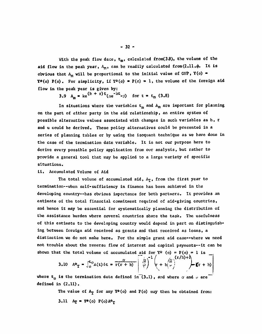
With the peak flow dace tm calculated from(38) the volume of the
aid flow in the peak year Am can be readily calculated from(2114 It is
obvious that Am will be proportional to the initial value of GUP Y(o) shy
Y(o) P(o) For simplicity ifY(o) = P(o) - 1 the volume of the foreign aid
flow in the peak year is given by
39 Am - ke (h + r)t (eht-P) for t = t m (38)
In situations where the variables tm and Am are important for planning
on the part of either party in the aid relationship an entire system of
possible alternative values associated with changes in such variables as h r
and u could be derived These policy alternatives could be presented in a
series of planning tables or by using the isoquant technique as we have done in
the case of the termination date variable It is not our purpose here to
derive every possible policy application from our analysis but rather to
provide a general tool that may be applied to a large variety of specific
situations
i Accumulated Volume of Aid
The total volume of accumulated aid AT from the first year to
termination--when self-sufficiency in finance has been achieved in the
developing country--has obvious importance for both partners It provides an
estimate of the total financial commitment required of aid-giving countries
and hence it may be essential for systematically planning the distribution of
the assistance burden where several countries share the task The usefulness
of this estimate to the developing country would depend in part on distinguishshy
ing between foreign aid received as grants and that received as loans a
distinction we do not make here For the simple grant aid case--where we need
not trouble about the reverse flow of interest and capital payments--it can be
shown that the total volume of accumulated aid for Y (o) = P(o)= I is -i
310 AT = deg A(t)6t = r(r + h) (r + hL + h)
where to is the termination date defined in-31) and where a and p are-
defined in (211)
The value of AT for any Y(o) and P(o) may then be obtained from
311 AT - Y(o) P(o)AT
- 33 -
If all or part of the foreigu aid inflow is contracted on a loan
basis this method will produce an underestimate of the total repayment obligashy
tions incurred when termination date is reachad The formula above could be
revised however to allow accurate calculation of total repayment obligations
at termination date if a constant rate of interest were applicable Similarly
using equation (211) the analysis could be extended to estimation of the
duration of the repayment period after termination date on the basis of the
capital export capacity that will then be built into the system
C Numerical Examples
The analysis of this section can conceivably be applied to all aidshy
receiving countries but this task requires estimation of values for the five
parameters s(o) u k h and r The present authors are now engaged in a
statistical investigation of these parameters for many underdeveloped countries
Our preliminary work in this area has emphasized the difficulties of deriving
sound estimates but nevertheless the research will be extended to include
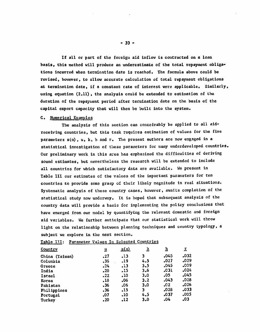
all countries for which satisfactory data are available We present in
Table III our estimates of the values of the important parameters for ten
countries to provide some grasp of their likely magnitude in real situations
Systematic analysis of these country cases however awaits completion of the
statistical study now underway It is hoped that subsequent analysis of the
country data will provide a basis for implementing the policy conclusions that
have emerged from our model by quantifying the relevant domestic and foreign
aid variables We further anticipate that our statistical work will throw
light on the relationship between planning techniques and country typology a
subject we explore in the next section
Table III Parameter Values In Selected Countries
Country u s(o) k h r
China (Taiwan) 27 13 3 043 032 Columbia 36 19 45 027 029 Greece 24 13 35 045 009 India 20 15 36 031 024 Israel 22 10 30 05 045 Korea 18 06 32 043 028 Pakistan 36 06 30 02 026 Philippines 36 15 3 028 033 Portugal 07 10 45 037 005 Turkey 20 12 30 04 03
- 34 -
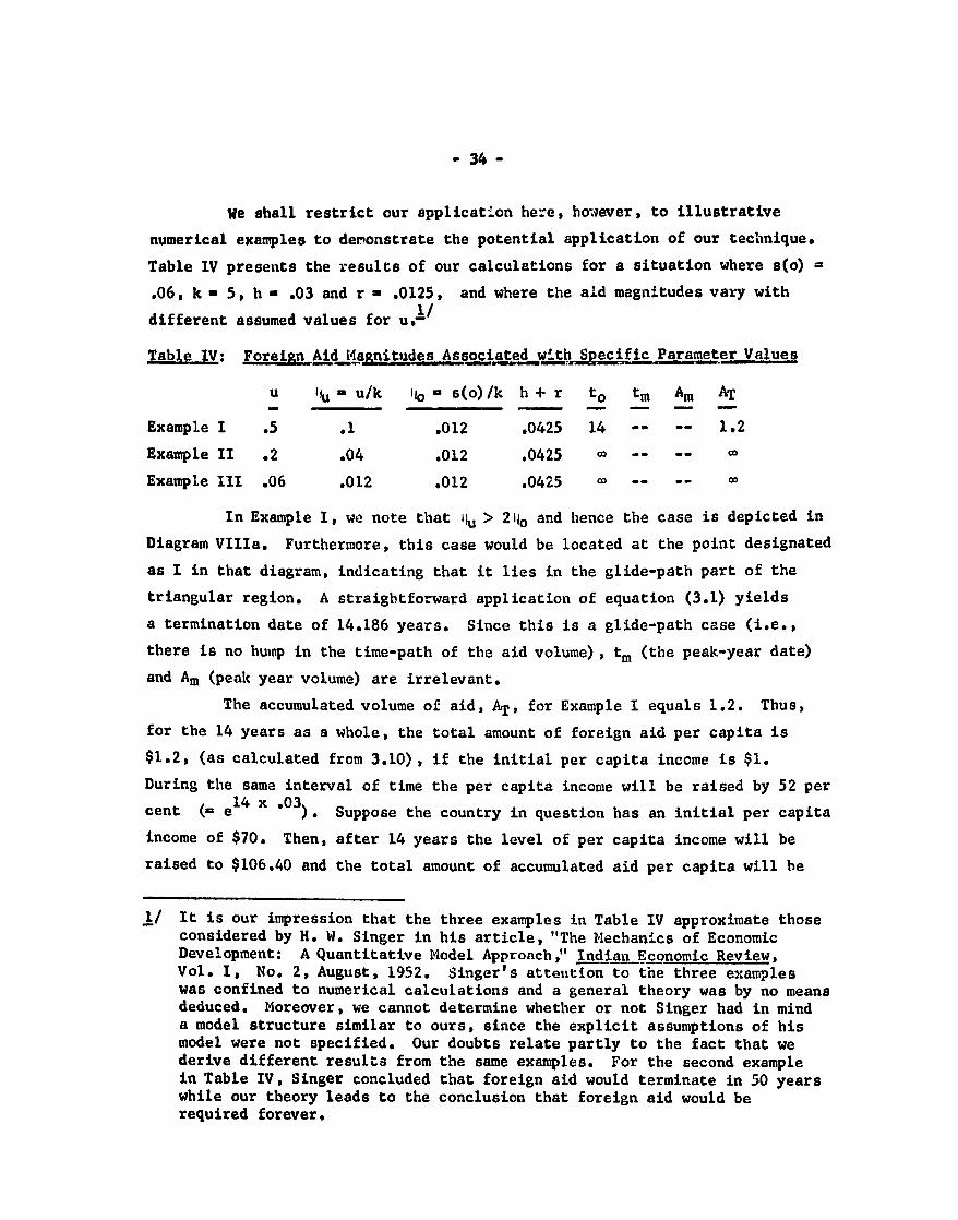
We shall restrict our application here however to illustrative
numerical examples to deronstrate the potential application of our technique
Table IV presents the results of our calculations for a situation where s(o)
06 k - 5 h - 03 and r - 0125 and where the aid magnitudes vary with
different assumed values for us 1
Table IV Foreign Aid Magnitudes Associated wh Values
u It - uk lio - s(o)k h + r to tm Am AT
Example I 5 1 012 0425 14 12 Example II 2 04 012 0425 0
Example 111 06 012 012 0425 Ca
In Example I we note that ij gt 2110 and hence the case is depicted in
Diagram Vlla Furthermore this case would be located at the point designated
as I in that diagram indicating that it lies in the glide-path part of the
triangular region A straightforward application of equation (31) yields a termination date of 14186 years Since this is a glide-path case (ie
there is no hump in the time-path of the aid volume) tm (the peak-year date)
and Am (peak year volume) are irrelevant
The accumulated volume of aid AT for Example I equals 12 Thus for the 14 years as a whole the total amount of foreign aid per capita is
$12 (as calculated from 310) if the initial per capita income is $1
During the same interval of time the per capita income will be raised by 52 per 14 cent (- e x 03) Suppose the country in question has an initial per capita
income of $70 Then after 14 years the level of per capita income will be raised to $10640 and the total amount of accumulated aid per capita will be
1 It is our impression that the three examples in Table IV approximate those considered by H W Singer in his article The Mechanics of Economic Development A Quantitative Model Approach Indian Economic Review Vol I No 2 August 1952 Singers attention to the three examples was confined to numerical calculations and a general theory was by no means deduced Moreover we cannot determine whether or not Singer had in mind a model structure similar to ours since the explicit assumptions of his model were not specified Our doubts relate partly to the fact that we derive different results from the same examples For the second example in Table IV Singer concluded that foreign aid would terminate in 50 years while our theory leads to the conclusion that foreign aid would be required forever
- 35 shy
$84 If the country has an initial population of 30 million (eg the
Philippines) the total aid will be $252 billion or an average annual volume
of about $180 million At the termination of foreign aid the average
propensity to save will have been raised from the initial level of 6 per cent
to 21 per cent as can be readily calculated from equation (28)
Examples II and III are clearly what we describe as unfavorable or
t3 cases represented by points II and III in Diagrams Villa and b In our
terms of reference gap-narrowing aid is required to move these cases into
the 2 region where finite values to the aid magnitudes can be determined
IV IMPLICATIONS FOR PLANNING TAXONOMY
Cooperation between aid-giving and aid-receiving countries in the
development planning field has become a natural step in the evolution of
patterns of economic assistance Both partners in the relationship have
sought to apply techniques for assessing the future prospects of the developing
economy and for maximizing growth by rationally allocating resources over time
In focusing on the relationship between external capital resources and the
behavior of domestic financial capacity our analysis has direct relevance for
both domestic development planning and foreign assistance policy
The formal analysis above predicts that the conditions which determine
self-help capacity may produce a variety of results and our statistical
investigation confirms that such variety is found in the real world We are
thus led to view the policy issues in terms of the more general problem of
planning methodology an area in which much work remains to be done Rather
than exploring this general problem in depth hwever we limit our discussion
to the specific problem of planning taxonomy as it bears upon the special
cases characterized by the conditions we have defined for the triangular
region In this region the important policy questions concern the choice of
strategy and tactics appropriate for devising a plan which will satisfy the
key elements in the self-help criterion given relatively adverse initial
conditions To recapitulate the foreign aid gap must be narrowed to reduce
the duration and volume of foreign assistance requirements to reasonable
magnitudes as well as to provide adequate--and politically acceptable--targets
for the growth of per capita income and consumption
- 36 -
To explore these issues for the triangular region we utilize the
parameters from the preceding analysis This venture into relatively uncharted
normative territory however requires that the framework of our analysis be
broadened to allow the variation of the parameters u s(o) and k previously
treated as constants We can now envisage cooperative gap-narrowing efforts
between the aid partners as encompassing measures to increase u or s(o)
(ie greater domestic austerity) or to reduce k (ie to enhance the
productivity of capital) To limit the scope of the discussion however we
concentrate on the planning implications of allowiag u the per capita
marginal savings ratio to vary This critical parameter appears to be
sensitive to such routine public policies as taxation and monetary control and
in using u to increase domestic austerity the planner can explicitly take
account of per capita consumptioa in considering what share of per capita
GNP increments are to be mobilized as savings Of the several possible foreign
aid variables we select only the termination date for examination in this
context Hence there are four planning variables to be considered in discussing
planning taxonomy and the policy model which follows u (PI4SR) r (population
growth rate) h (target growth rate of per capita GNP) and to (termination
date for foreign aid)
If for example the value of u were given and a population growth
rate were specified for the triangular region it is obvious that h the optishy
mum target and to the minimum termination date will be determined In this
special case we might speak of the pair of planning variables u and r as
the instrument variables (ie the variable u reflecting domestic austerity
measures and r reflecting population control measures) and h and to as target
variables (ie certain specific objectives to be pursued) We note however
that such classification can be made only after one pair of planning variables
are specified and the other pair accordingly can be determined This
suggests the need for a more comprehensive taxonomy of planning variables to
enable selection of the relevant variables on the basis of economic and
institutional characteristics of individual societies For the four planning
variables in our present system several alternative combinations between
independent variables (whose values are given by extra-model considerations)
and dependent variables (whose values are determined endogenously) are possible
- 37 -
The taxonomic approach to planning therefore requires a systematic listing of all possible specifications for the variables included in the system Table V presents such a listing for the four variables under discussion The application of one of the six alternative combinations inTable V to a particular society in the triangular region requires conscious evaluation of planning limitations and opportunities that grow out of the societys total institutional framework It serves the planner well to remember that these broader institutional problems are not specified by the model structure and hence a particular policy model should not be applied indiscriminately to all societiesl
Table V Taxonomy of Planning for Triangular Region
Typeof Society
ase Population Sub-variables Independent Number Variable i _ ariables
la) Unrelenting Austerity-reluctant u r to p h lb) Population Aid-restrictive to r h u
nc) Growth Target-fixation h r to u
2a) Population Austerity-flexible h to ru
2b) Control- i Aid-flexible h u r t o 2c) Sensitive Target-flexible to u r h
The study of planning methodology from the taxonomic approach has not yet been developed adequately however to permit specification of independent and dependent vartables for a given society on a systematic basis
1 A more systematic investigation of the planning methodology issue wouldprobably lead to the concli1on that in the application of a model such as we present to an actual situatix several or all of the alternative combinations of variables must be used ina process of successive approxishymation An application of this type might eventually culminate in linearprogramming techniques to determine the maximum feasible solution byiteration (eg the simplex method) We doubt however that highlysophisticated techniques of this kind will be useful for this particulardevelopment planning problem until further progress has been made insolving planning taxonomy and data problems For these reasons we haveavoided a highly technical investigation in this part of our inquiry
- 38 -
It is difficult to go much beyond an attempt to determine (from the planners
general knowledge about the institutional constraints that appear to exist in
his particular society) which potential planning variables are likely to be
subject to his influence In other words the planner can do little more than
to explicitly distinguish between variables over whose specific values he has
some degree of choice (dependent variables) and those for which his society
imposes such an unyielding preference for a particular value that the planner
is left with no choice (independent variables) It is likely that there is
considerable diversity of the types of target and instrument variables
available for planning purposes in different societies What is needed
therefore is an attempt to systematically classify societies on the basis
of the types of variables that are likely to be available for planning
purposes in unique combinations of institutional conditions
In light of the above discussion the classification scheme in
Table V may be viewed as an attempt to relate planning methods to types of
societies The policy issues to which it is addressed concern the choice of
strategy for avoiding the dismal conclusions reached for the triangular region
This region is characterized by high population pressure hence we draw a
basic distinction between the prospects for economies in this region depending
on whether or not the population problem can be directly attacked through
control measures Where existing social values or administrative incapacity
present unyielding obstacles we consider the rate of population growth r
to be an independent variable and we describe the three possible cases (la b
and c in Table V) as unrelenting population growth cases If in addition
domestic austerity programs cannot be introduced perhaps because of population
pressure itself we have case la and the society type also takes on the
characteristic of being austerity-reluctant Similarly the names given the
other society types are based n tho rolac which tho paramatta ru to-and
h are likely to play for planning purposes ie whether the institutional
framework will reduce them to independent variables or allow the planner some
influence in determining their value
The onstraints imposed by institutional forces may be unduly
restrictive the first exercise above may be inadequate to establish a
meaningful planning process A part of the planning strategy might then be
- 39 shy
concerned with a pre-conditioa1 ng effort to remove social or political conshystraints which obstruct changes in the value of critical planning variables In other words planning may include an institutional change function to alter the distribution of independent and dependent variables In some situations this longer-run approach may be the only realistic implementation of the gapshynarrowing strategy
Where as incase la of Table V we have an unrelenting population force austerity-reluctant type society our analysis of the triangular region leads to the conclusion that a satisfactory rate of growth cannot be achieved even though the foreign aid variable can be manipulated Despite the availability of two planning variables (to and h) planning per se is likely to be ineffective for promoting progress beyond avery modest rate of growth A longer gap-narrowing strategy devoted to unfreezing one or both of the critical planning variables r and u appears to be the only escape
Our model may be used to demonstrate how the above approach to planning methodology can be given operational significance The problem is to devise a method which relates the important planning variables in a systematic way to enable the planner to consider all alternative combinations relevant to his particular society We recall that the application is made only for the triangular region where the problem of choice of gap-narrowing strategy is critical because population pressure severely limits the range of feasible development programs
We assume that the initial average propensity to save s(o) and the capital-output ratio are given and for illustrative purposes we use the specific values of s(o) = 10 and k = 3 Given these initial conditions a triangular region case will exist if the rate of population growth r exceeds the initial growth rate of capital ie 1o = s(o)k or 03331 Letting the value of the PMSR u vary from this value to its maximum value of unity a system of optimum target curves (similar to the curve XMY in Diagram V) can be derived In Diagram IX (where as in Diagrams IV V VII and
j This case has some empirical validity Table III shows that this situation exactly matches the parameter values for Israel and ourpreliminary statistical work on other countries indicates that several Latin American and Asian countries will show relatively similar valuesTable III also suggests that the triangular region condition (rgt 1ia)holds for Korea and Pakistan although their population growth rates are below those used in this example
- 40-
VIII values of r are shown on the vertical axis and h on the horizontal)
these optimum target curves are shown as the system of backward bending
curves all beginning from the point li - 0333 on the vertical axis and
each indexed by a specific value of u Termination date isoquants are shlown
as the system of positively sloped curves indexed with specific foreign aid
termination dates in years It will be remembered that minimum termination dates are associated with every point on the optimum target cuives (ie
for any given combination of h and r) and hence these isoquants may be termed the minimum termination date isoquants The two systems of isoquants
are presented in full in Diagram IX although only a small part of the map
is relevant to planning problems in the real world The likely range of population growth rate variation begins at 33 per cent by definition of
the triangular region for our assumed values and we would not expect it to
rise above 4 12 or 5 per cent
The analysis is further adapted for actual planning decisions in
Table VI which gives a more explicit listing of numerical values derived
from Diagram IX Several possible values of the PMSR u are shown in the left-hand margin while values for the population growth rate r from 335
to 5 per cent are given in the top margin Each cell relating the variables u and r contains two numbers the top number representing the termination
date to and the bracketed lower number representing the target rate of growth of per capita GNP h The values given for to and h in the cells are
respectively the minimum termination date end the optimum target associated
with the given values of u and r (Thus reading from left to right in each
row in Table VI is equivalent to an upward movement along a backward
bending u isoquant in Diagram IX and reading downward in a column equivalent
to movement along a horizontal line in the Diagram)
- 41 -
Table VI Selected Relationships in Policy Model for Triangular Region
r (1) (2) (3) (4) (5)
PrSR - 0335 r - 035 r- 04 r - 045 r- 05 Line 1
(1) u - 15 62 (027)
102 (057)
(2) u - 20 31 43 67 107
(07) (8) (12) (127) 914np
(3) u - 30 16 2 61_4 (37) 4 2(247)
(4) u - 40 11 17 (8) (30)
(5) u - 50 8 3-- 0
(6) u= 90 4 (167)
(7) u = 100 4 (45)
Termination date longer than last termination date in the same row
Not available from IBM Tabulation
Table VI contains two broken auxiliary lines labelled line 1 and
line 2 Cells which lie above line 1 contain tdrget rates of growth of per
capita GNP which are less than 1 per cent per year rates which in our
judgment are too low to be used as satisfactory planning targets Cells
which lie above line 2 contain termination dates exceeding 45 years--which
we consider to be too remote to qualify for foreign assistance While
admitting that the lines are arbitrarily drawa from extra-model considerations
it is our position that only those cells which lie below both line 1 and line 2
represent reasonable and feasible choices available to the planner
i~ It should be pointed out here that effective planning inevitably involves value judgments of this kind to bridge the gap between analysis and reality In fact we view the essence of the science of economic planning as an effort to reduce extra-model considerations to a minimum and to make value judgments identifiable and explicit In the application of a planning model such as we present in Diagram IX the exogenous considerations may be consciously introduced in a straightforward manner
- 42 -
The major conclusion emerging from this analysis (which applies only
to real situations appronimating the conditions we assume ie s(o) - 10 k - 3 and r gt 033) is that domestic austerity programs are crucial to
achieve a satisfactory target and a reasonable termination date for foreign
assistance More specifically domestic austerity measures must ensure that the PHSR be at least 30 per cent for when it is 20 per cent or less either
the target growth rate is unduly low or the termination date for foreign assistance is unreasonably long The importance of domestic austerity
(giving the assumed conditions) can be seen as the PDISR u is raised from 20 per cent to 30 per cent reducing termination dates by more than 50 per cent while simultaneously allowing substantial increases in targets
Nine entries in Table VI are circledl to denote possibilities with realistic population growth rates (45 per cent or less) and satisfactory
targets (14 to 4 per cent) combined with relatively high levels of domestic
austerity (PMSR from 30 to 50) and feasible foreign assistance termination
dates(from 12-30 years) While PMSR values from 30 to 50 appear high itmust be remembered that domestic austerity of this degree would make 50 per cent to 70 per cent of increases in per capita GNP available for increased
Per capita consumption Thus given a disposition to practice adequate domestic austerity our conclusion for even the difficult triangular cases has a marked optimistic flavor A gradual rise in per capita consumption is
consistent with a reasonable termination for foreign assistance
1 Although the numerical entries inTable VI were calculated from about 10 pages of printed IBDI computer tabulations precise values could not be calculated for the cells marked Approximate values for these cells however can be obtained by interpolation
2 Entries in Column (I)where r = 035 require explanation Here we find that increases in the PMSR u reduce termination dates but fail t-o raise targets to satisfactory levels even though the rate of population growthis the lowest shown in the table In the last entry tabulated in this column the extremely high u of 90 is associated with a very short termination date (4years) and a very modest target (16 per cent) This paradoxical result indicates that the minimum termination date and optimum target concepts are not usefully applied in this special situation In practice such countries could probably afford a longer termination date enabling them to adopt a higher target
- 43 -
This relatively optimistic conclusion for countries with unfavorable initial conditions deserves emphasis- In short even where population
pressure is severe and the initial srwings rate low adequate self-help measures of the austerity type could provide conditions under which foreign assistance would consistently raise both per capita GNP and consumption
Equally significant these increases would be adequate to accelerate selfshysufficiency of domestic finance rapidly enough to yield a reasonable time perspective from the viewpoint of the aid-giving country This optimistic conclusion we submit provides strong incentives for vigorous domestic planning efforts to combine austerity with foreign economic assistance An adequate rate of growth of per capita income (a key element of the self-help
criterion)-icould be maintained thus eliciting popular support for the development program by continuous improvement inpresent low consumption standards while simultaneously insuring that foreign assistaLce can be terminated within a reasonable period of time Both features are likely to comfort those who levy the foreign aid burden on citizens in developeo countries
It is also reassuring to find that an apparently feasible austerity program (requiring a PMSR of 30 to 50 per cent of per capita income increases)
yields a satisfactory prognosis for countries confronting relatively great
obstacles to development This implies that the many countries where the
initial relationship between population growth and domestic savings capacity is more favorable (our parallelogram region) could meet the self-help criterion with less domestic austerity efforts (a lower PMSR) Our estimates inTable III suggest that seven of the ten countries listed--China (Taiwan) Columbia Greece India the Philippines Portugal and Turkey--fall in this more favorable
category
l The other aid variables (eg the required volume of accumulated foreignassistance over time) could be estimated by routine application of our formulae above to investigate their behavior under the assumed conditions
See page 1 item iii of key elements in the self-help criterion
- 44 -
V POLICY CONCLUSIONS
In addition to the applications of our analysis to joint development planning efforts in the preceding section there are important implications
for both the economic and political foundations of foreign aid policy Foreign
economic assistance--wbether in the form of grants or loans--has an unfortunate history of political difficulties in both developed and undershy
developed countries In the case of the United States Lhe leading provider
of foreign aid Congressional doubts have placed foreign assistance programs
in growing jeopardy Political attacks have centered upon the dubious
leverage effects of aid in helping countries to become independent of largeshyscale foreign economic assistance in a reasonable period of time Impatience has been a matter of both nebulous time horizons for terminating aid and the magnitude of the task- Similarly there are many cases where acceptance of foreign aid has created internal dissension in underdeveloped countries
coupled with charges of political subservience to the large provLders of foreign assistance For these and other reasons we feel that it is
important for both parties in the assistance relationship to give explicit
consideration to the quantitative aspects of foreign aid through the application of methods such as we have presented in this paper
In planning for effective use of eccnomic assistance we find it essential that the aid-giving country be able to distinguish clearly between countries which qualify for gap-filling assistance and those where the foreign
aid gap is so large and permanent that the first order of business must be
1 There are innumerable statements to this effect in recent Congressionaldocuments See for example Cogressional Record - Senate June 13 1963 pp 10219-10228 Ibid November 4 1963 pp 19942-19963 CongressionalRecord - House August 20 1963 pp 14618-14652 Ibid August 21 1963 pp 14675-14707 One statement succinctly puts the problem to which much of the discussion pointed The dilemma of foreign aid has alwaysbeen this How can the United States live up to its tradition of humanitarian ideals and its world leadership in the cause of freedom-shyfreedom from hunger disease and ignorance as well as from politicaloppression--without casting itself as the mere administrat- of a vast welfare prorampouring endlessly from the American cornucouia into the bottomless gulf of world needs (underlining ours) 14r Cameron Congressional Record - House August 15 1963 p 14249
- 45 shy
narrowing of the gap Past failures inU S assistance are at least partly a matter of inadequate or imprecise allocation criteria incapable of sharply drawing this basic distinction- Moreover aid programs have failed to classify the relative opportunities for success by distinguishing among varying degrees of self-help capability within these broad categories As a result it is likely that much foreign aid has flowed to countries where
failure was built into assistance programs by a combination of faulty assistance strategy and unfavorable initial conditions in the recipient
country
Our analysis provides operational criteria for avoiding past errors of this kind Properly applied the methods we propose allow objective judgments about the economic prospects of countries requesting assistance as
well as systematic comparison of societies for formulating specific assistance strategies These objective standards could be used to supplement rule-ofshy
the-thumb and wise man evaluation of aid recipients--often largely from
intuition or hunches We caution hwever that the economic information
yielded by application of our techniques must be used with discretion It is important to understand what lies behind significantly different results for individual economies Noreover frequent re-calculation of the critical variables and parameters would be desirable both to test whether or not
changes have occurred and to take advantage of improvement in the scope and
1 Congress has recognized and criticized the absence of clear-cut operationalcriteria See for example statement by Mr Cederberg quoting and endorsing a minority report We have been troubled by continuing evidence of lack of reasonable criteria in the selection of the recipients of our aid Congressional Record - House August 21 1963 p 14695 See also Senator Ernest Gruenings comments in Report of a Stud of United States Foreign Aid in the liddle Eastern and African Countries pp 465-472 where the assertion is made (p 471) What is desperately needed in the AID program is a set of criteria for determining which nations in the free world are worthy of receiving U S foreign economic assistance These criteria should be widely published And even more importantthey should be rigidly followed Gruening is clearly thinking of the concept of self-help we are willing to give economic assistance to underdeveloped nations of the Free World provided--and only provided-shythey are willing at the same time to help themselves Ibid p 470
- 46 shy
accuracy of underlying statistical data If our methods were to be applied
to the global problem of U S aid allocation complete coverage of all aidshy
recipient countries would be necessary Our own survey of the data suggests
however that the statistical basis for such a comprehensive effort does not
yet exist Nevertheless the analysis can already be applied to many important
developing countries which receive large amounts of U S assistance
The qualitative analysis in this paper offers important lessons for
the general principles of foreign aid policy as well as for specific aid
strategies A first major conclusion with general import is that gap-filling
aid will in fact lead to the predicted termination date if and only if the
inflow of foreign capital assistance is adequate to consistently fill the gap
Only under these conditions will potential domestic savings actually
materialize from self-help efforts through the per capita marginal savings-
GNP relationship If this proposition is firmly grasped and such opportunities
for success are correctly identified the political case for a consistent and
adequate foreign-aid program will be strengthened The effective rejoinder to the impatient critic of U S economic aid therefore is that temerity and
short-run thrift in the foreign-aid business are likely to lead to interminable
aid involvement with countries which could soon become independent of our
assistance through an enlightened program On the other hand we must
re-emphasize a second conclusion a fear that appears to haunt many members
of Congress Where countries do not meet the gap-filling criterion even
large-scale capital assistance will fail to spark a self-help effort capable
of terminating the need for foreign aid within a reasonable time- If
economic assistance is to be given to countries of this type its major purpose
should be to assist these countries in undertaking development planning
programs to enhance self-help capacity
I This fear is reflected in much of the recent Congressional discussion on foreign aid Senator Church expressed the general apprehension as it applies to Latin America Pointing to evidence of stagnation in these economies he goes on to say instead of the situation improving it is growing worse We do not have enough money in this country We could pour all the wealth of the United States into Latin America and it would all go into a sinkhole and not stabilize those countries Congressional Record - Senate November 13 1963 p 20654
- 47 -
It should be borne in mind that economic analysis offers only a partial yet important contribution to the solution of foreign aid policy problems Enlightened self-interest must inevitably play an important role in dispensing foreign aid particularly when aid is unilateral rather than international- Political and security considerations will continue to be mixed with economic allocation criteria but even the non-economic criteria
can be more meaningfully applied with better tools for evaluating economic performance The self-help criterion which has been given specific operational meaning in the preceding analysis is an example of an allocation principle
with both economic and political implications Domestic austerity programs and judicious use of savings are likely to depend on political and
institutional changes such as land reform enlarged economic opportunity and improved incentives to work save and invest The economic manifestations
of self-help therefore reflect the political performance of a society in terms of its capacity to disseminate economic goals incentives and opportunities widely enough to promote economic progress
1 The influential Clay Report phrases the relationship between economic and political cilteria in strong clear terms Whether a country ought to receive aid from the U S is a question of our enlightened selfshyinterest however the kind and basis of aid provided thereafter--except when paramount military security or other extraordinary circumstances are involved--are questions to be determined on economic grounds Here as in other instances the U S must establish sound benchmarks for its own performance and stick to them whatever the vagarics of ephemeral world opinion Report to the President of the United States from the Committee to Strengtben the Security of the Free World - The Scope and Distribution of United States Mjilitary and Economic Assistance ProgramsDepartment of State Washington 25 D C March 20 1963 page 6
APPENDIX
Section I
Integrating (12b) with respect to t we have
AI1) S uY + c
= where c isthe integration constant Let t o in (A1l) we have
c = S(O) uy(o) = (S(o)) - uY(o))P(o) = (s(o) Y(o) - uY(o))P(o)
= (s(o) - u) Y(o)
and hence (14a) is proved The model of section I is defined by 1labc)
12ab) and 13) To solve for the growth path we have
Al 2) a-AWdt 2 =dSdt by (1la)
b dYdt = (dKdt)k by (1lb)
c dPdt = rP by (11c)
d dSdt = (dSdt - rS)P (by differentiating dSdt =
d(SP)dt)
= e dYdt (dYdt - rY)P (by differentiating dYdt
d(YP)dt)
Substituting A12bde in (12b) we obtain the following second order linear
differential equation
A13) a d2Kdt 2 + B dKdt + C = o where
=b B -(r + uk)
= c C ruk
Solving the characteristic equation
=A14) x2 + Bx + C o
the two characteristic roots are
Al5) a xI uk (= U)
b x2 r
A2
and hence the growth path of capital stock is
e qu tAl6) K(t) =1 + j2 ert
The growth paths of gross national product and savings are then
=Al 7) a Y (4k)enut + (42k) ert (by 1ib)
= b S = dKdt 11 ue u +4 2 r ert
Substituting t o this pair of equations we= in have
=Al8) a kY(o) 241
b S(o) = 41 Iu + -2 r
which can be solved to obtain the values of 1 and 42 as indicated in (19)
in the text The time path of Y C S and K(t) as shown in 18abce in
the text are thus established
For the three cases R1 R2 R3 identified in (17) in the text the sign
of 1 and cj2 are thus
Al 9) a the favorable case ( m gt 1) o lt d1 and o lt 12
b the intermediate case (mlt o) I lt o and o lt 42
c The unfavorable case (olt m lt ) lt and 2 lt o
From these conditions and (AI6) we see that the most favorable case is the
only case in which the capital stock can increase in the long run This is
obvious for the most favorable cases as both 41 and C2 are positive For the
two other cases the long run growth rate of capital are approximately
Al10) a K=O 1 enut (for a 1 lt o for the intermediary case)
b K =a-2 ert (for 2 lt o for the unfavorable case)
A3
Thus in either case the capital stock becomes negative after a
time span as stated in the theorem in the text The above finding may be
checked by investigating the per capita income (Y) the per capita savings
(S) and per capita consumptions (C) though time The direction of change
of Y C and S can be investigated through differentiating (18abc) in
the text with respect to time
=A111) a dYdt ckl(u- r) e (nur)t
kP(o)
b dCdt = l (l-u) (Ou-r) e(Vur)t
= l1 u P(o)( j u - rc dSdt r ) e (Tu-r)t
P(o)
Notice that the sign of all the coefficients are positive for the most
favorable case and are negative for the intermediate case and for the unshy
favorable case Thus Y S and C monotonically increase from the
beginning for the most favorable case and monotonically decrease for the
other cases as we have asserted in the theorem in the text From (l8a)
and (Al lla) the rate of increase of per capita income is
A112) 0= (u(u-r) -r)tY u e u
1 + e(1ur)tm shy
=For t = o and t 10 respectively we have
AI13) a y(o) = no-r
b Ty () u-r
confirming our choices for names of 1 and Iu in (15) in the text Differshy
entiating (Al 12) with respect to u and to t respectively we have by
r ) t = Lwriting e(u~ e
A4
Al 14) a dTY)d - (deg-r) eL l-l)+(eL-)n(1 + eL m2 m k k(-r)
m 1
b d1y = L (o-r)(1-r)(l - m ) dt (1 + eLm)2
m
which are positive for the favorable case (RI) Al 4a proves 110 in the
text while Al 14b proves an assertion in part 1 of the theorem in the txt
Section II
Differentiating (2lla) with respect to time
(h +A21) a dAdt = r)t -ht )(h + r) -oheh and hence K(o) e -e eb dAdt h+r ht gt he-lit lt -ht
o (hr-(h+r h ----rAe~ h
(h+r)(3 -(+hr)e ht
The time path of the term on the right hand side is plotted in diagram Al
The curve begins from a value (l+hr)(= uk - (h+r)) (at point X) which
is positive for the intermediate case The value of (= uk - s(o)k)
which is also positive is represented by a horizontal line such as UU and
VV From A2lb we see that in the latter case (VV) which is the 4 case
defined in (213a) in the text dA lt o for all t In the former case (UU) dt
which is the case defined in (213b) in the text there exists a critishy2
cal time point t such that
A22) a dA dt lt tFtgt0o fort m
b olt dA for t lt t dt m
=and hence A takes on a maximum value at t t The boundary line between m
the two regions 1 and 6 in dliagram IV in the text (ie equation 212)
A5
can be rewritten as
= A23) a 1u- 10 (u - (h+r))(l + v) or
= =b h+r = r(l + v) h(l + lv) wI u + w2 0 where
C V 1C w 1 w2 - and l+v l+v
=d v hr
which is (37) in the text Notice that wI and w2 form a system of weights
(ie w gt o and wI + W2 1) with values completely determined by v = hr
The right hand side of (A23b) is thus a weight average of Tu and o with
u gt 10 From these relations we immediately conclude
A24) a v - implies wI - w2 - gt and h+r -- 1u(with h
r -- o)
b v - o implies w -o w2 - 1Iand h+r -gt 0 (with h o r 0)
c lt h+r lt0 u
Thus in diaram IV in the text we see that the boundary curve XZY passes
through point Y(X) on the horizontal (vertical) axis and lies entirely in
the 2 region We also have dw1 dv = I(l+v) 2 gt o and dw2dv = -I(l+v) 2 lt o
and hence (A23) implies that h+r and h are both increasing functions of v
Moving from point X to the right on XZY in diagram IV we see that as v
increases the value of h increases and the curve itself intersects higher
h+r - isoquant Furthermore it is obvious that the curve must eventually
be negatively sloped as point Y is approached (ie as v )-r)To see
whether the boundary curve may be positively sloped near X (i e as v 0o)
we compute drdv from (A23b)
A25) drdv = (1 + v) H dwl + q dw2 (W u + w dv dvshy _
(I + v)2
A6
Thus we have
A26) drdv - (9 - v) 9
Near point X (ie v --- ) o) we see
=A27) drd 0 Tu lt 2 deg (for v hr - o)
and hence the boundary curve increases near the point X if and only if TIu
i worc LhItLI Lice as high as 1 0 Furthermore if this condition is not
satisfied (ie if 1o lt 1] lt 21o) (A26) implies
A28) drdv lt o for all v gt o (when 11o lt IIIlt 211 )
Thus the entire boundary curve is negatively sloped Conversely (ie when
= u gt 2To ) the equality in (A2 6) implies that a critical value of v vc gt o
can be solved ie
=A29) v = hr 1 - 2110 gt o (for 1u gt 211o)
such that u
A210) a drdv gt t for v lt vc wwhen TI gt 211 deg
b drdv lt o for v gt vc) u
=and hence the boundary curve reaches a unique maximum value where hr 1 shy
21oh u This proves (35) and (36) in the text as summarized in diagram
VIII
A7
Section III
Let us first investigate the behavior of the to-isoquants near the point X
in diagrun As shown in (3 1) in the text the equation of the isoquants
is
-- -
The coordinate for the point X is (h o r = s(o)k) Letdh and a f
denote deviations from the point X The value of L in the neighborhood
of X is by A31
~ (a -f()7P)(41-jJ-lt -z 17 -
Using Lhoupitc1 Rule we have for a fixed value of X _- _ 1--
R dsoa r o
Referring to diagram V see that as long as point X is approachedwe
A8
from within the 42 region -gt -1 and hence A33 implies that a positive
finite value will be approached More specifically
5 A4 t0 = i t gt-I4J
A34a) (A34c) shows that moving along the boundary line XX (YX) upward
(downward) toward X leads to a limiting value of zero (infinity) for t
(A34b) shows that as gt - 1 varies the limiting value of t may appraoch I)
any finite positive value This proves propertyl in the text ie the
point X is the beginning point of all the to-isoquants
The shapes of isoquants of diagram V can be further verified by the values
of t for all points on the horizontal line segment XY on the horizontal
=axis In the first place the value of to at point X (r o h = s(o)k)
=is obviously zero and the value of to at point Y (r o h = hk) is obshy
viously infinity Thus to show all the to-isoquants will terminate on the
line segment XY we only have to show that the value of to monotonically
increase as a point moves from X to Y along XY For r = o we have
co ) = i)
---n-PP_
A9
It is our purpose to show A gt B for (r = o s(o)k lt h lt uk) We have
for the point
= ( ____)- i - gt
Thus to show that A gt B for other points on XY (diagram V ) we only need
to show dAdh gt dBdh We have for r = o
A07)
cdh y
Thus we have shown that moving from X to Y in diagram V the termination
date increases monotomically from o (at X) to infinity (at Y) Hence all
the to-isoquants must terminate on the line segment XY This proves property 5
To investigate the slope of the isoquants we compute
14A I
A1O
Thus we have
A - - __
C C71 h66L)
Let us define a critical value of Tm by
A 31o) 0 (
I
- lty - - - gtsi
which is (32) defined in the text In case to lt Tmwe have
A3 ) -o lt(Tii =~ gtx lt lt~i -~ - ltlt
and hence (A39b) implies -- lt o This proves that all the to-isoquants withdh
a termination date less than Tm will be negatively sloped
Conversely let to be a termination date which is greater than Tm (ie
togt T) Then
A4 3 9 A( lt~ lt
1
All
The number G(to) can thus be represented by a point such as Z between X
-and Y on the horizontal axis in diagram V Let the 450 line Z r be
drawn Equation (A39b) shows that the to -isoquant will have a positive
(negative) slope if it lies to the left (right) of Zr However we know LA
the to-isoquant does lie to the left of Zr because it passei through the
poiuL X Hence it must have a positively sloped portion The fact that it
must always terminate on the horizontal axis between X and Y implies that
it must also have a negatively sloped portion Thus the to -isoquant
reaches a maximum point on the straight line Zr ie
Thus we have proved the signifishy
cance of the critical terminal date Tm defined in (32) in the text
The equation for the optimum termination date locus (XN- diagram V) is
obtained directly from to - in (A39a) and (A31) ie
which can also be written in the parametric form
+ 3 -
Substituting (A34a) in (A34b) we have h to- ln( to) which may again be
Al2
substituted in (A34a) to yield
Using these equations we can easily prove
6316) - shy
which shows that the optimal target locus passes through point X and Y in
diagram V
The point M on the optimum target locus is the point when h is a maximum
To find the value of r and h at M we compute
Aj 37) t
Substituting (A317b) in (A315) immediately yields
43)
ALshy
which is (3 4) in the text
DIA RWIS
(Foreign Assistance and Self-Help A Reanpraisal of nevelonLent Finance)
Diagram Page
Diagram I D1
Diagram II Dl
Diagram III a b c D2
Diagram IV D3
Diagram V Di
Dinqram VI P5
Diagram VII P6
Diagram VIII a b D5
Din-rari IX 7
Dingran Al D5
A B lt
fqvOrchz 44M-C-AampZ 4-44A
DIAGYAM I - 5Mng 4
A3
x
Vy
-DIA-CniAMa SOjpf 1YcMd- Saampna 4 wfiokL
Al
AA
aircJ- -
A A I
I II 2I0
0 i I1i I i i
I i i Ogg
L -L --- shy
z~ Rew~nI Ronvi
- - -2 t-2--e
A CGRAM I11 Sildic4ntRegions b45ea on 6 aviar
IL -
-
fk
K ~1 7
1
z
yt
)
2
gt
-VI
2
II
j--
-_
A
_
_ _ _ _
____-__-_____-_-________
(-1lu + 2 flo
T)
j2 -- (-lt2-n
- - - h
0
I I Al
VII
r - VT Diagtram A]
6
I
Y
I
2 o
00
1I9 0
00shy
1
i 5 - J I - - I
0 3 5
K
I
~ I
I
-t
-
ll
I
-
-I
-
fl bull
___ - -- - X-shy I
- -
~ i
A V~
D-ibull
1
bull1
i
I Th2
T II
bull _
05 -gt1
i_
771 -~ -
Ibull

HAS BEEN EVALUATED AS SUBSTANDARD COPY FORTHIS DOCUMENT
ROUTINE REPRODUCTION EFFORTS IN AIDW TO OBTAIN A MORE
HAVE NOT BEEN SUCCESSFULACCEPTABLE COPY OF THE DOCUMENT
WE HAVE CHOSEN TO REPRODUCE THEDESPITE THIS DISADVANTAGE
OF THE SUBJECT TREATED AND TO MAKE THEDOCUMENT BECAUSE
DISCERNIBLE INFORMATION AVAILABLE
CENTER FOR DEVELOPMENT PLANNING National Planning Association
1525 18th Street N W
Washington 6 D C
FOREIGN ASSISTANCE AND SELF-HELP
A Reappraisal of Development Finance
by
John C H Fel Douglas S Paauw
M-7720 Dev Plan 63-1 December 1963
Until recently little thought was given to the relationship between foreign assistance and the mobilization of domestic savings to finance economic development The Foreign Assistance Act of 1961 served to stimulate interest in this problem by enunciating the criterion of self-help I a condition for U S foreign aid with which Congress and the Administration has become preoccupied Official interest in selfshyhelp finds its counterpart in recent academic thinking
The purpose of an international program of aid to underdevelopedcour-ies is to accelerate their economic development up to a point where a satisfactory rate of growth can be achieved on a self-sustainingasis Thus the general aim of aid is to provide in each underdeveloped country a positive incentive for maximum national effort to increase its rate of growth The increase in income savings and investment which aid indirectly makes possible will shorten the time it takes to achieve selfshysustaining growth Ecor2 mic progress is measured primarily by increases in income per head
While both practical men and scholars seem to agree on the importance of self-help this notion has remained more a slogan than cn operational
tool Unless this appealing shibboleth is enriched with analytical content its programming significance is likely to be elusive To give content to self-help as a criterion for foreign aid several key elemers in the dynamics of the assistance relationship must be identified for analysis
These key elements include (i) the interaction between foreign aid and domestic austerity efforts (ii) assurance that a reasonable termination date be built into the assistance program (iii) evidence that foreign aid will achieve its primary economic objective of providing an adequate rate of growth of per capita income and (iv) confidence that the accumulated
j the President shall take into accountthe extent to which the recipient country isdemonstrating a clear determination to take effective self-help measures Public Law 87-195 87th Congress S 1983 September 4 1961 p 4
P N Rosenstein-Rodan International Aid for Underdeveloped CountriesThe Review of Economics and Statistics Vol XLIII Number 2 May 1961 p 107 (underlining supplied by present authors) See also Charles Wolf Jr Savings and the Measurement of Self-Hell in De elZvingCountries The Rand Corporation Memorandum R4-3586-ISA 1963
-2shy
volume and annual flow of foreign aid to satisfy these conditions will be
within reason It is the purpose of this paper to derive allocation
criteria by relating foreign aid to domestic savings capacity We seek
to integrate the above elements into an analytical system relevant to
analysis of the development process as a whole rather than treating the
elements as isolated phenomena
We submit that allocation criteria must have the operational
capacity of providing numerical answers to such important assistance
questions as the duration of aid the time path of its flow the peak year
volume the accumulated value over time and the required domestin savings
to achieve the prime objective of foreign assistance The heterogeneity
of underdeveloped countries presents an additional difficulty The criteria
must have the power to discriminate among qualitative characteristics by
country to shed light upon the type of assistance strategy most appropriate
for individual countries Of special importance is the need for distinguishshy
ing between conditions under which countries almost automatically qualify
for capital assistance and conditions which require a more selective
discretionary assistance program The criteria we evolve from the subshy
sequent analysis satisfy these requirements
Professor Rosenstein-Rodan recently published global estimates of
capital inflow requirements for economic development of underdeveloped
countries- The familiar Harrod-Domar model served as the analytical
framework for his estimates while the national austerity effort concept
for mobilizing additional savings as income rises was based on a Keynesianshy
type marginal propensity to save While we accept the general outlines of
the Harrod-Domar model we have doubts about the suitability of the
Keynesian-type saving function for analyzing the savings potential of
underdeveloped countries Our objections are based on the observed fact
that per capita consumption standards in these countries are so near the
subsistence level that a realistic domestic austerity program must take
into account the difficulty of further lowering per capita consumption levels
We prefer therefore to utilize a savings function which relates increments
I International Aid loc cit pp 107-138 Rosenstein-Rodans study provides a wealth of empirical information as well as many intuitive insights However the analytical component of the study is peripheral to the central issues investigated in the present paper
- 3 shy
in per capita savings to increments in per canita income We shall refer to this concept as the oer canita marginal savings ratio abbreviated as PMSR It will be shown that the postulation of a PM3R savings function in place of the Keynesian savings assumption is both more realistic for development planning and a more satisfactory basis for answering the self-help questions
we have posed above
In the first section we investigate the formal logic of the growth of a closed economy in the framework of our revision of the Harrod-Domar
model Using the PMSR saving function we examine the short and long-run dynamic behavior of the closed economy Our primary purpose is to present a few important growth theory concepts which are central to our subsequent analysis In the second section we proceed to apply our model to an open
economy in which domestic and foreign savings are assumed to be the two possible sources of finance for the investment requirements for growth We apply this analysis to clarify the meaning of self-help by demonstrating
potentialities for achieving self-sustained and self-financed growth The qualitative analysis of this section is supplemented by quantitative analysis in Section III where we develop methods to provide numerical answers to the
various important planning questions raised earlier (eg duration volume and peak year of foreign aid flows) Section IV is devoted to a brief
exploration of the uncharted area of planning tax=onomy We propose an approach by which the policy implications of our analysis may be applied to a wide variety of institutional situations In Section V we stress the major conclusions emerging from our study as they bear upon U S foreign
aid policy and development planning in underdeveloped countries The more technical material for all sections is presented in the Niathematical Appendix
I THE PER CAPITA SAVINGS MODEL THE CLOSED ECONOMY
We begin by recapitulating the following assumptions for the traditional Harrod-Domar model using Ix to denote the rate of growth of
the time variable x (ie(6x6t)c)
lla) 1K - SK (accounting relationship between IIK K and S where I - S)
b) Y - Kk (production condition where k is the capitalshyoutput ratio)
-4shy
c) li = r (constant population growth rate)
d) S = sY (aggregate savings function)
The four basic eccnomic variables are gross national product (Y) -shyhereafter abbreviated as GNP -- capital stock (K) total population (P)
and gross national savings (S) and the three parameters are the capitalshy
output ratio (k) the population growth rate (r) and the average propensity
to save (s) In the closed economy investment (I) equals gross national
savings (S) To construct a per capita savings model we retain the first
three relationships above (lla b and c) but we break with the Harrod-Domar
tradition by replacing the aggregate savings function S = sY Letting Y(=YP)
and S(- SP) denote respectively per capita GNP and per capita savings the
saving behavior hypotheses in our model are
12a) S(o) = s(o)Y(o) and
b) 6S6t = u 5Y6t
We depart from the Harrod-Domar model therefore by rejecting the assumption that a constant average propensity to save s holds for all time
periods Rather given an initial average propensity to save s(o) (in 12a)
we assume that increments in per capita savings are a constant fraction of
increments in per capita GNP (l2b) where the proportionality factor u will
be termed the per capita marginal savings ratio (PIASR) If the value of u lies
between o and 1 (ie o lt u lt 1) increments in per capita GNP will lead to
both increased per capita consumption and increased per capita savings We
further assume that u is greater than s(o) ie the per capita marginal
savings ratio exceeds the initial average propensity to save
13 s(o) lt u lt 1
As we shall see in our later statistical analysis (see Table III of
SectionIIu this assumption is satisfied by the recent experience of most
underdeveloped countries
It can be shown (see Appendix) that the saving behavior assumption
(12) of our model implies that per capita saving S and the average
I Gross national savings S will denote savings from gross national product ie internal savings throughout the paper
-5shy
propensity to save s are respectively
14a) S = uY - Y(o) (u - s(o))
b) s = SY = Y u - (u - Is(o)) Y(o)Y
Thus in the special case u s(o) we have S = s(o)Y or
S - s(o)Y (lld) which demonstrates that the Harrod-Dowar model is a
special case of our modei In other words the Harrod-Domar model applies
only to the special case where the average propensity to save and the per
capita marginal savings ratio are equal Our assumption (13) implies
that as long as per capita GNP (Y) increases the average propensity to
save s is in fact an increasing function through time which can be
easily seen from (l4b)
To facilitate our later analysis we define the following concepts
in terms of the primary parameters of our model
15a) iio s(o)k (initial growth rate of GNP and capital)
b) 1Iu uk (long-run growth rate of capital and GNP)C) m -r
110 - r (domestic austerity index)
Intuitively io(representing the rate of growth of GNP and capital
in the Harrod-Domar model) is the initial growth rate of GNP and capital while1 I is the long-run rate of growth of GNP and capital in our model-
Accordingly the numerator of m is the long-run rate of growth of per capita
GNP while the denominator is the initial rate of growth of per capita GNP
We note that (13) implies
16 1Io lt I
Thus in case r lt o m is positive and the greater the disparity
between the PMSR u and the initial average propensity to save s(o) the
greater will be the value of m For this reason we shall refer to m as the
domestic austerity index
Let us indicate the value of 110 and the value of 1ju by points A and B
on the horizontal axis r representing the population growth rate (see
Diagram I) The two points A and B divide the horizontal axis into three
1 For justification of these choices of names see equation (Al13) in the Appendix
-6shy
regions RI R2 and R3 depending on the comparntive magnitude of the actual
value of r relative to i and a The received doctrine of high populationo
pressure as a barrier to growth is intuitively apparent in this analysis
hence we shall refer to the three cases as
l7a) R (favorable case) o lt r lt 1 implying I lt m
b) R2 iI r lt ijimplying m lt (intermediate case) o lt o
c) R3 (unfavorable case) I1lt r implying o lt m lt 1
We accept the familiar indicators cf success and failure to
evaluate these cased per capita GNP Y per capita coiLsumIptlon C and
per capita savings S We shall say that an economys growth performance
is successful if all these magnitudes increase in the long run Conversely
we construe failure to occur if these magnitudes decrease in the long-run
In Case Rl the favorable case the Harrod-Domar model would lead
us to conclude successful development could be achieved since the population
growth rate r is less than the growth rate of GNP IVand capital 1K Conversely in case R2 the intermediate case and Case R3 the unfavorable
case the Harrod-Domar model would predict failure since the rate of
population growth r exceeds the rate of growth of GNP I and capital 1K
An interesting question arises can a count-y where failure is
predicted by the Harrod-Domar model achieve success by practising austerity
Is it possible to reverse the predicted failure by adopting a high PPSR even
though the average propensity to save is initially low Intuitively if a
country devotes nearly all of its increments in per capita GNP to finance
investment (dissipating little on consumption) one would epect that per
capita GNP and consumption would eventually increase (even though initially
declining) Yet we reach the surprising conclusion that this is not the
case in the closed economy in fact we may state the following theorem
1) In Case R1 the favorable case Y S C and K monotonically
increase from the very beginning of the process Furthermore
the rate of increase of per capita GNP livL4also monotonically
increases
2) In Cases R2 and R3 the intermediate and unfavorable cases Y
St and C monotonically decrease moreover capital stock K
will become negative after a finite time span because
disinvestment will occur
-7-
These conclusions can readily be verified by the following equations describing the time path of the various indicators mentioned in the above theorem (see Appendix)
18a) Y = YP = [akP(o)Ie( u - r)t + a2kP(o) (per capita GNP)
b C = CP = [a(1 - u)kP(o)le(1U - r)t + v2(l-kr)kP(o) (per capita consumption)
c) S = Y - S (per cepita saving)
r)tr) e(iu shy(jIu shym - + e( i - r)t (rate of growth of per
capita GNP)
e) K(t) ale ut + 2efrt (capital stock)
where
19a) Q- = kY (o)m
=b) a2 m - l)kY(o)m
Part i of the above theorem does not cause surprise since the Harrod-Domar model predicts success even where u (the per capita marginal savings ratio) equals s(o) and s remains constant over time However ifu is greater than s(o) the average propensity to save will be increasing through time (l4b) making success even iore obvious In fact it can be shown (see Appendi) that the higher the value of u the higher will be the rate of growth of per capita GNP (l8d) ie
110 gt o for the favorable case
confirming our intuitive notion that greater domestic austerity promotes more rapid growth
Part 2 of the theorem emphasizes the futility of a domestic austerity program i1L an economy where high population pressure exists in combination with a low initial average propensity to save One might even go so far as to depict this as a futile domestic ausLrity situation Failure will always occur regardless of stringent programis to rciae the PiASR For
- 8 shy
such an economy our analysis points to the policy conclusion that in a closed economy population control is the only escape
The economic eplanation of this strong and intuitively paradoxical conclusion is apparent when we realize that per capita GNP is not increasing from the outset because of population pressure Hence the critical austerity variable PIISR has no positive force because there are no positive GNP increments from which per capita saving increments may be mobilized A high PIISR yields additional savings therefore only where per capita GNUp in fact rises
For a country in this situation -- where high population pressure precludes success from even extreme domestic sacrifice -- foreign aid is seen to be strategic in sparking the growth process This external push is indispensable to prod the economy into yielding initial increases in per capita GNP so that domestic austerity -- the high PNSR -- can be made to yield its potential contributions to a cumulative process of raising domestic savings investment and per capita GNP It is this problem on which we focus in the next section
II DOMESTIC SAVINGS VERSUS FOREIGN ASSISTANCE THE OPEN ECONOY A The Harrod-Domar Model
We begin our investigation of combining foreign assistance with domestic savings by exploring the conclusions which can be derived from the familiar Harrod-Domar model We introduce the possibility of adding foreign resources to finance investment I by distinguishing between two sources of finance domestic savings (S)and foreign savings (A)I
Combined with the other basic assumptions the Harrod-Domar Open Economy Model can be described by the following system of equations
j Harrod extends his analysis to an open economy in his equation GC shy s - bwhere G is the grcwth rate (the increment of total production in anyunit period expressed as a fraction of total production) C is theincrease in capital divided by the increment in output (the capitaloutput ratid) s is the fraction of income saved and b is the balance of trade expressed as a fraction of income This formulation howeveris applied only to analyze the impact of the foreign balance on aggregate demand R F Harrod Towards A Dynamic Economics London 1952 Chapter 4
-9shy
2a) I S + A
b) Y- Kk 11c) K IK
d) - r
e) S= sY
We now turn to a problem that will concern us throughout the
remainder of our analysis Let a target rate of growth of per capita GNP h
be given ie
- (ie Y - Y(o)eht)22 1 h
Our investigation will center upon the flow of foreign savings (A)through
time that will be required to advance and sustain such a target We may
think of the target as a politically established goal deemed necessary by
the political leadership as indeed we find in most underdeveloped countries
Alternatively one could consider the adoption of such a target to be the
rate of growth of per capita income that appears to be feasible on the basis
of such considerations as absorptive capacity and the existence of certain
obstacles to growth
From the above assumptions we see that the rate of growth of the
gross national product is
23a) Ij = - 4 + lip - 17p + k h + r (see 22 and 2ld)
b) Y Y(o)e(h + r)t
Since the capital output ratio (k)is constant (2lb) implies that
capital stock must grow at the same rate as Y and hence we have
24 11K = h + r
which may be interpreted as stating that the needed rate of growth of capital
and the demand for investment finance is determined by the population
growth rate (r)and the target growth rate of per capita income (h)
Substituting (24) (2la) and (2lb) in (21c) we have
25 k(h + r) = SY + AY
which states that the demand for investment finance (investment requirements)
I Rosenstein-Rodan embraces the latter concept of the target rate of growth International Aid loc cit pp 111-113
- 10 shy
must be met either from savings supplied internally S or externally from
foreign savings A Notice that the first term on the right-hand side is the
average propensity to save while the second term will be referred to as the
aid-income ratio
It is apparent that equation 25 is generally valid in the sense of
being independent of any domestic saving behavior hypothesis For the Harrod-
Domar savings assumption (2le) this equation reduces to the following
special case
26 h = (s - rk)k + (AY)k
To investigate the relationship between the target rate of growth
of per capita GNP b and the aid-income ratio AY let us represent h on
the vertical axis and AY on the horizontal axis in Diagram II For fired
values of s r and k equation (26) is shown as a straight line with a slope
1k and with a vertical intercept sk - r This diagram demonstrates that
as a country raises its target rate of growth of per capita GNP h (moving
upward on the vertical axis) a higher aid-income ratio AY will be
required Conversely as more foreign savings (a higher aid-income ratio)
become available a higher target h can be sustained
There are essentially two types of dynamic behavior in this open
model as represented by the parallel lines I and II in Diagram II The two
cases are differentiated by the fact that line I has a positive vertical
intercept and line II has a negative vertical intercept
27a) sk gt r Favorable Case (line I)
b) sik lt r Unfavorable Case (line II)
The favorable case is characterized by low population pressure and
(27a) indicates that per capita GNP will increase (at the rate shown as the
vertical distance OX) in the absence of foreign savings If a target higher
(lower) than OX is specified the country will import (export) capital
forever
Conversely in the unfavorable case where population pressure is
great per capita GNP will decrease by OY in the absence of foreign savings
The horizontal distance OZ is the aid-income ratio which would yield
- 11 shy
stationary per capita GNP (h = o) If the aid-income ratio is greater than
(less than) OZ per capita GNP will rise (fall)
Two important conclusions from this application of the Harrod-
Domar model require emphasis First if a country needs a given aid-income
ratio to sustain a specified target h it will require this level of foreigin
savings in Reretuum Assuming that foreign aid is a major component of
foreign savings we see that the very logic of the Harrod-Domar model
precludes a realistic analysis of the problem of a termination date for
foreign aid Our formulation below fills this major gap in existing theory
Secondly when a certain aid-income ratio is required to achieve a given
target h the absolute volume of foreign aid will grow exponentially at the
rate h + r We consider these to be rather unrealistic features Yet the
Harrod-Domar model has provided us with a framework for analysis which we
now proceed to build upon
B The PMVSROpen Economv Model
To recapitulate our argument in Section I our only revision - albeit
a critical one - of the Harrod-Domar model is to replace the savings behavior
assumption (2le) with our assumption based on PMSR presented in (12)
We believe that the model we develop on this basis constitutes an important
step toward realism in planning the finance of economic development We
demonstrate that our method allows both parties in the aid relationship to
analyze in precise terms the growth of domestic saving capacity and hence
foreign savings requirements for reaching self-sufficiency in the developing
country
The savings behavior hypotheses based on PMSR (12) lead to an
average propensity to save given by (l4b) hence the availability of
domestic savings becomes
s - u u -hs(O)28) e ht
if the target rate of growth of per capita GNP is given by (22) When
(28) is substituted in (25) the needed aid-income ratio AY can be
determined residually as
- [u - h()29) AY - k(h + r)
e
- 12 -
In Diagram ila let time be measured on the horizontal axis and
let the aid-income ratio be measured on the vertical axis in order to plot
the time path of the aid-income ratio AY The following steps are needed
to interpret the diagram
a) Let point I on the vertical axis denote the constant value
of k(h + r) ie total investment requirements
b) Let the time path of the average propensity to save s in
(28) be represented by the positively sloped curve
starting from point B on the vertical axis Notice the
value indicated at point B is the initial average propensity
to save s(o) and that this curve increases monotonically
approaching asymtotically a horizontal line A A where
point A denotes the value of the PMSR ie u This curve
shows that when per capita GNP is growing at a constant
rate h the value of th average propensity to save rises
from its initial value to approach the value of u the P1ISR
c) Let a horizontal line through point I be drawn to intersect
the average propensity to save curve at point T
d) The value of AY will then be represented by the shaded
distance between the two curves or the negatively-sloped
curve starting from point C on the vertical axis
Notice points A and B divide the vertical axis into three regions
T1 2 and b in which point I may fall Making use of the concepts
o -i s(o)k initial growth rate of capital and i = uk long-run growth
rate of capital as defined in (l5a b) of the previous section the three
regions may be precisely defined as
210a) l (favorable case) h + r lt s(o)k -P 1l0
b) 2 (intermediate case) nolt h + r lt uk Ju
c) 3 (unfavorable case) Iju lt h + r
The dynamic behavior of AY the aid-income ratio for the three
cases is represented in Diagrams lia IlIb and lc The favorable case
21 Diagram IIb represents a combination of a low population growth rate r
- 13 shy
and an unambitious target h yielding a situation where no foreign savings
are required in fact the contry will export capital from the outset
Capital exports will constitute an increasing fraction of gross national
product as AY approaches a constant value in the long-run
In the intermediate case 2 shown in Diagram IlIla the country
will need foreign savings at first but there will be a finite termination
date shown by point T (or to on the time axis) After this point has been
reached the country will be able to export capital and to repay whatever
loans were contracted during the period foreign savings were imported
In the unfavorable case 3 shown in Diagram IlIc we see that
foreign savings will be required indefinitely because of a combination of a
high target h and a high population growth rate r The aid-income ratio
AY will eventually approach a constant value implying that the absolute
volume of foreign savings required will grow at a constant rate ie the
rate of growth of gross national product h + r
Before proceeding with further analysis we digress to ecamine the
policy implications in terms of the three cases Obviously Case l the
favorable case need not concern us since domestic savings are adequate to
finance domestic investment requirements to maintain the targeted growth
rate and even to provide a surplus for capital export from the outset Hence
there is no problem of combining foreign and domestic savings indeed with
rare exceptions (eg Nalaysia) we do not envisage underdeveloped countries
falling into this case
The distinction between Case 2 and Case 3 has important policy
significance In the intermediate Case 2 there is a definite termination
date for foreign savings and beyond this date adequate savings will be
generated domestically to provide for loan repayment (in addition to meeting
domestic investment requirements) In other words foreign aid for a finite
period promotes self-help by stimulating progress to the point where selfshy
financed growth becomes possible and the capacity to repay foreign debt
incurred in the process of reaching this point will accelerate Foreign aid
supplied in this situation may be thought of as gap-filling aid since it
allows the country to move toward financial self-sufficiency if the gap
between investment requirements and domestic savings is actually filled during
- 14 shy
the crucial transition period
The unfavorable case 93 does not share these properties Even
though te gap is filled by foreign savings there will be no progress toward
a termination date toward achieving loan repayment capacity or even toward
reducing the rate of flow of foreign savings Our analysis suggests that a
country will remain in this unfavorable situation unless it can reverse the
condition qu lt (h + r) into (h + r) lt 1u-If the initial conditions match
those of Case 3 therefore the strategy appropriate to the interests of
both parties in an aid relationship should be aimed at moving the country
to a more favorable situation The basic operational principle of the
strategy would consist of the recipient country adopting domestic policy
measures to narrow the gap sufficiently to produce a reasonable termination
date Hence we refer to this as the gap-naKrowin aid case
We note that our approach in this section leads toward a more
meaningful interpretation of self-help We define self-help as a foreign
assistance-stimulated program of domestic austerity to generate an adequate
supply of domestic financial resources over time to ensure reasonable and
finite dimensions to the foreign assistance program The distinction between
gap-filling and gap-narrowing foreign aid prcqides a realistic basis for
applying the self-help criterion In the case of countries qualifying for
gap-filling aid an adequate flow of foreign savings will enable the economy
to progress toward self-sufficiency in development finance merely as a
result of adequate capital assistance In other words foreign aid of this
type may be viewed as automatically assisting the countrys austerity
program to fulfill the self-help condition without careful administrative
supervision This is tantamount to finding adequate absorptive capacity
in the sense that gap-filling aid is absorbed to enhance the capabilities
l Note that in the closed economy analysis in the first section the
crucial condition for success is r lt io ie the population growth rate must be less than the initial growth rate of capital while in this open economy case the crucial condition for a finite termination date is (h + r) lt u ie comparison between h + r and the long-run growth of capital
Policies appropriate to this strategy are discussed in Section IV
- 15 shy
of the recipient country to generate a sustained and cumulative growth process from domestic resources- This type of absorptive capacity does not exist in the other case 3 where foreign aid fails to automatically contribute to improvement of domestic financial capabilities
In this latter case therefore the more demanding assistance task of narrowing the gap between growth requirements and domestic financial capacity is implied if the self-help criterion is to be met Capital assistance alone will merely plug a long-run gap and permit a country to live beyond its means - without generating leverage effects toward greater self-help The policy conclusion is that foreign aid of a package-deal type is required in this case conditions for progress toward greater self-help must be analyzed and specified The recipient country should be induced to accept a firm commitment to narrow the gap so that foreign aid will begin to spark the growth of domestic savings capacity If a program of foreign assistance cannot be devised to satisfy the self-help criterion by narrowing the gap in such countries there are strong economic grounds for withholding assistance- The task of providing gap-narrowing aid therefore requires a more flexible and imaginative approach than in the gap-filling case Here the art of providing useful assistance requires sophistication and diplomacy and costs and administrative demands are likely to be high It follows that foreign technical assistance has a special role here since we would envisage a need for expert external advice in assisting the country to devise and implement domestic policy measures for changing tbe adverse initial conditions
1 We note that Professor Rosenstein-Rodan also uses this condition as oneof several interpretations of absorptive capacity See P N Rosenstein-Rodan Determining the Need for and Planning the Use of External ResourcesOrganization Planning and Programming for Economic Development ScienceTechnology and Development United States Papers Prepared for the UnitedNations Conference on the Application of Science and Technology for theBenefit of the Less Develop ed Areas Vol VIII pp 70-71
2 We wish to emphasize however that political and security considerationsfall outside this analysis and that in the real world non-economic criteria may turn out to be of overriding importance
- 16 -
To continue with the analysis of the time path of foreign aid it is
apparent that the behavior of the aid variables is determined completely by
the five parameters in our model s(o) u k h and r The significance of
these parameters is more clearly exhibited in Diagram IV where the target
rate of growth of per capita GNP h is measured on the horizontal axis and
the rate of population growth r on the vertical axis A system of parallel
45 degree lines such as XX and YY are drawn to denote h + r isoquants
Let the initial growth rate of capital Io and the long-run rate of growth
of capital li be marked off on the horizontal atis by the points X and Y
respectively determining two particular isoquants XX and YY These two
straight lines divide the first quadrant into three regions The definitions
of the three cases l 2 and 3 given in (210) show that the intermediate
case 2 is the region defined by the trapezoid XYYX while the favorable
case 1 (unfavorable case 13) is the region below (above) this trapezoid
The combined effect of growing population pressure and more
ambitious targets can be represented by the movement of a point in Diagram IV
from the origin outward in the northeast direction traversing the three
regions D1 t2 and b successively Hence such movement produces the
foreign aid consequences described above for the three X cases The
significance of our model as a natural extension of the Harrod-Domar model can
be seen once again from Diagram IV Equation (28) shows that the Harrod-
Domar special case obtains when u equals s(o) This can be interpreted to
hold in Diagram IV when points X and Y coincide which would obviously
eliminate the intermediate region 2 This shows again that a meaningful
termination date cannot be derived from the Harrod-Domar approach since
the two remaining cases I and b call either for no aid or perpetual aid
Hence the significance of u becomes apparent we are able to identify and
analyze the important case 2 which qualifies for gap-filling aid only
when u differs from s(o) A foreign aid termination date is a meaningful
phenomenon only in this case this in turn results from our introducing the
possibility of considering varying degrees of domestic austerity as measured
by different values for the PMSR or u The question of whether or not
foreign aid promotes self-help in raising domestic savings capacity has
- 17 shy
special importance We see now that there is a positive relationship
between the two in only one of the three regionLs the one adurmbrated by
traditional analysis of the Harrod-Domar type
In addition to the termination date dimension of the problem it
is important for both aid-giving and aid-receiving countries to plan in
advance the volume of aid requirements and how it is likely to change over
time More deliberate evaluation of long-run commitments and obligations
become possible with such knowledge and the danger of mere year-to-year
improvised programs is reduced If applied such knowledge could make for
a more rational use of foreign aid by reducing uncertainties for both parties
For discussion of this problem we return to Diagram IV We
already know that in region I no foreign aid is needed and in region 3
foreign aid will increase monotonically Concentrating on the intermediate
case 2 therefore we derive the volume of foreign aid through time as
A = [k(h + r) - (u - (u - s(o)e ht)]Y by (29)
= [k(h + r) - u + (u - s(o)e-ht y(o)e(h + r)t oby (23b)
(lh + r - uk + (uk - z(o)k)eht]IK(o)e(h + r)t by (21b) and hence
21la) A = K(o)e(h + r)t (e-ht 0) where
o= =b) a Iu1- uk - s(o)k
c) P 16 i= uk- (h+ r)
To see the direction of change in A it will be shown in the
Appendix that the region 2 has two subregions 2 and D2 divided by a
boundary curve XZY in Diagram IV given by the following equation2
212) t = f(l + hr)
when at and 5 are defined in (21lbc) In other words the
two subregions are defined by
I Heuristically since a is the difference between the long-run growth rate of capital and the initial growth rate of capital it may be termed the potential difference in capital growth rates Given k and s(o) the magitude of this potential difference is directly related to the national austerity index as measured by u (PMSR)
2 It will be shown in the Appendix that the boundary line passes through the points X and Y The exact shape of the boundary line and its economic significance will be discussed in the next section
- 18 shy
213a) 2 (glide path case) a lt 3(l + hr)
b) 2 (hump-scaling case) P(1 + hr) lt a
Although there is a finite termination date for both sub-regions
there is a difference in the shape of the time-path of the volume of foreign
2 the volume of aid first rises to a maximum andaid A In sub-region
The aid volume conclusions therefore can be distinguishedthen decreases
more picturesquely as a egt case for the sub-region 2 and a humpshy
scalinR case for 2 In the glide-path case the process of growth of
domestic savings capacity operates to continuously reduce foreign aid
requirements and external assistance may be viewed as gliding down a path
progressively nearer self-sufficiency No particular aid counsel is needed
here since the end of the task is in sight and the burden of assistance
continuously declines Both conditions are attractive to countries providing
assistance
In the hump-scaling case on the other hand although the
termination of aid is a known prospect the peculiar behavior of the needed
volume of aid may raise doubts from the aid-giving countrys viewpoint
The hump of a maximum volume of assistance must be scaled before a glideshy
path phase to ultimate success appears This analysis therefore has
special value for distinguishing among countries where an increasing annual
volume of assistance is required With the assurance that a country falls
into sub-region the fear of an ever-growing volume of assistance that
will never terminate may be allayed In this special case we counsel patience
This incidentally justifies a big initial push approach to foreign assistshy
ance for countries where austerity programs exist but where the hard road
to self-sustained growth involves growing foreign aid before the self-help
response begins to reduce the required volume
III QUANTITATIVE ASPECTS OF PLANNING FOR DEVELOPMENT ASSISTANCE
As the analysis has proceeded we have pointed to implications for
improving the principles of development assistance strategy applicable to
both aid-giving and aid-receiving countries In the previous sections the
underlying theory was mainly based on qualitative analysis in this section
= 19 shy
a more quantitative basis is supplied This amplification leads to further
clarification of the self-help concept and it also provides methods for anshy
alyzing alternative time and volume patterns of foreign assistance
Solutions to the quantitative problems raised in this section therefore
are essential for strengthening the theoretical basis underlying development
assistance policy (which we consider in Sections IV and V) as well as for
the statistical implementation of our model
A Quantitative Analysis of Termination Date
We have consistently stressed the Importance of the planned
termination date for foreign assistance Analysis of the intermediate case
2 in the previous section provided a basis for relating termination date to the self-help criterion and for giving concrete meaning to self-help as
a measure of country performance We recall that termination date estimation
is relevant only for this case In the favorable case I no foreign
assistance is needed while in the unfavorable case 3 foreign assistance
will never terminate The termination date can be determined by setting the
aid-income ratio (AY) in 29 equal to zero
n- u-3 1 j s(o) -l I In [u k(h + r) ]31 to h- l - - h ln ( )
where i= uk - s(o)k and j - uk - (h+ r) as defined above in (21lbc)
We know that aO gt I for the intermediate case hence a positive termination
date to can always be found
Diagram V is a reproduction of Diagram IV in the previous section
In the trapezoid XYYX which represents the intermediate case Y2 we draw
parallel h + r isoquants and also a system of to (termination date) isoquants
the latter determined from equation 31 This equation indicates that
upward movement along any specific h + r isoquant will increase the termination
date to since ln(cy0) remains unchanged and h decreases Geometrically this
can be seen from the fact that upward movement along an h + r isoquant cuts
successively higher termination date (to) isoquants This implies that the
slope of the to isoquant is greater than -1 Economic meaning can be given
to this fact by first noting that the slope of the to isoquant may be thought
of as a marginal rate of substitution between h and r leaving the termination
- 20 shy
date unchanged The fact that the marginal rate of substitution is greater
than -1 means that a reduction in the target rate of growth of per capita GNP
h of 5 per cent for example will fail to compensate for the termination
date lengthening effect of a 5 per cent increase in the rate of population
growth r Hence the numerical rate of population growth exerts greater
weight on the termination date than the per capita GNP growth target
This phenomenon may be explained by use of an additional diagram
In Diagram VI let Diagram lia be reproduced The time path of the average
propensity to save is given by the solid curve Bs and the horizontal line
beginning from I (determined by h + r) intersects Bs at point T the
termination date Supposing r increases by the value of A the termination
date is seen to be lengthened to the point To o Conversely if the value of
h is increased by A (raising point I to I) the termination date is raised
only to the point T since an increased value of h will according to equation
28 also raise the Bs curve (the average propensity to save) to the position
of the dotted Bs curve
The map of to isoquants which is defined in the trapeziid XYYX in
Diagram V has a number of important properties that will be useful to our
analysis These properties are rigorously deduced in the Appendix while it
suffices here to state them and to investigate their economic meaning
(P1) The boundary between regions i and 2 ie line XX may be construed
to be the first to isoguant with a zero termination date
Notice that along this boundary line h + r = o - s(o)ki- As we have
seen in terms of Diagram lIla this means that point I coincides with point B From this diagrammatic analysis it is apparent that in this boundary
situation a country will be self-supporting in investment finance
at the outset and that it will begin exporting capital in the second year
The first rise in the average propensity to save as it is pulled upward by the force of the PNSR operating through the initial increase in per capita GNP
provides a surplus of domestic savings over investment requirements
(P2) The boundary between regions 2 and 3 line YY may becqnstrued to be
the last to isouant Les the to joguant with an infinite termination date In Diagram Mliathis corresponds to the situation where point I
coincides with point A and foreign savings would be required forever Even
- 21 shy
when the full force of the PMSR becomes effective and the average propensity
to save approaches the PMSR domestic savings will be inadequate to finance
the high investment requirements (P3) The left-boundary of relin 2 line XY maybe construed to be an
extension of the infinite termination date isoquant definedin P2
According to P2 and P3 the entire isoquant with the infinite terminashy
tion date is the broken line XYY The economic significance of the segment
XY can be seen from the fact that it coincides with the vertical axis and
hence the target rate of per capita GNP growth h is zero This means that the PMSR is impotent Thus equation 28 is reduced to s - s(o) the Harrod-
Domar case where a constant average propensity to save continues through
time In the terms of reference in Diagram lia this situation would show the
average propensity to save through time as a straight horizontal line beginning
from point B rather than as an increasing curie Point I would lie above
point B and the vertical distance from horizontal parallel lines beginning
from I and B would show that foreign savings would be required for all time
(P4) The bottom boundary of region 2 line XY is a line along which
successive increases in the target h from X to Y will cut to isoguants
increasing from 0 at X to infinity at Y
This is the special case in which the rate of population growth r
is 0 ie population is stationary In terms of Diagram IlIla the height
of point I would be simply kh rather than k(h + r) As I rises from point B
to point A the termination date indicated by point T increases from zero
to infinity
(P5) All to isoguants begin from point X
This point X represents the special conditions h - o and r - s(o)k
which may be interpreted as the simplest Harrod-Domar case involving stable
per capita GNP with neither foreign savings nor capital export Domestic
savings are just adequate to maintain the constant rate of population growth
at a constant per capita GNP level a situation which might be described as a
self-sufficient stationary state
Diagram V may now be used to elucidate further several types of foreign
assistance situations in terms of termination dates We concentrate first
on cases falling in the vicinity of X marked off in the diagram by a small
- 22 shy
circle Countries within this circle are in a precarious situation Small
variations in the value of any important parameter will open the whole range
of possible foreign aid termination results A small favorable change - or
positive stimulus - within the system (such as a slight increase in the initial
savings rate s(o)p reduction of the population growth rate r or lowering
the capital-output ratio k) will reverse immediately a perpetual capital
import situation to one in which capital export will continue forever On the
other hand a slight unfavorable change - or negative shock - will lead to the
postponement of the termination date possibly to infinity even though the
country had previously been exporting capital It is difficult to specify
desirable foreign assistance policy relevant to this small circle beyond the
caveat that wariness is necessary Countries in this category show low or even
negative per capita GNP targets hardly consistent with development assistance
goals or the criterion of self-help since we know that the PRSR will be either
impotent or negative M1oreover the situation is highly volatile small variashy
tions in parameter values will produce drastic changes in aid requirements shy
as seen from the wide diversity of termination date possibilities Given the
present hazardous state of statistical information about underdeveloped
countries an attempt to apply our quantitative criteria here would run the
risk of large margins of error in projecting the foreign aid magnitudes
The target rate of growth h itself turns out to be a critical
variable for determining termination dates for foreign assistance While we
would normally expect a more ambitious target to lead to a postponement of
termination date it may come as a surprise to learn that for many realistic produce
cases a higher target will in fact pvee a shorter termination date
To introduce this unexpected result of our analysis the following property
of the to isoquant system in Diagram V may be stated
(P6) There is a critical value for a specific termination date isoauant
Tm such that all to isoguants__) are eatvely sloped for to lt Tm and
(b) reach a maximum point for Tm lt to
From properties PI P4 and P5 above it is apparent that the system of
to isoquants will begin from X with negatively sloped curves for small values
of to near XX However properties P2 and P3 imply that as the value of to
increases the isaquants will gradually shift upward approaching the shape
of the broken line Wwhen to becomes sufficiently large Hence there isX Y
- 23 shy
a critical termination date Tm associated with a specific isoquant that provides a boundary between a class of negatively sloping isoquants and a class of inverted U-shaped isoquants It is shown in the Appendix that the
value of Tm (the critical termination date or CTD) and hence the isoquant
corresponding to Tm (CTD isoquant) are
32a) Tm =Ia = Iil- 0 (critical termination date or CTD)
b) 1a = hr (aO)n (CTD-isoquant)
where a is as defined in 211b
Hence the value of Tm is completely determined by u s(o) and k For example where u - 20 s(o) = 10 and k = 33 Tm 33 years= In Diagram V the isoquant corresponding to Tm is indicated by the curve XZ
Using the above properties P1 to P6 wa can readily plot the contour map of the to isoquants as in Diagram V all isoquants begin at point X1 and terminate at a point on segment XY Higher isoquants indicate longer terminashytion dates from zero to infinity The isoquant XZZ is a boundary line dividing the contour lines into two types those below it are negatively
sloped and those above it have a maximum point With this characteristic of the to isoquant system in mind we can extend the analysis by drawing an auxiliary horizontal line XV through the point X in Diagram V This line
divides the 2 region into two sub-regions an upper triangle XVY and a lower parallelogram XXYV We refer to the first sub-region as the triangular region and any point belonging to it as a triangular case The
second sub-region is termed the parallelogram region and it contains
parallelogram cases It is now apparent that these situations are distinguished by the fact that in the parallelogram the termination date contour lines
decrease continuously while in the triangle all to contour lines lie above
the boundary isoquant XZZ and have a maximum point It is shown in the Appendix that the locus of the maximum points for to isoquants in the trishy
angular region is given by the equaticn
33 P in() = h
With u k and s(o) specified equation 33 determines a curve XMY in Diagram V which heuristically may be referred to as the optimum target locus Point M denotes the maximum value of h on the optimum target locus
- 24 shy
the coordinates of Mgiven by
34a) h - ae
b) r- 16- 2h - -W2e
where e (- 271828) is the basis of the natutal logarithm We
now proceed to analyze the economic significance of the two regions beginning
with the parallelogram XXYV
i The Parallelogram Region
The implications of the more straightforward parallelogram cases
follow from the fact that the to isoquants are all negatively sloped As we
would expect an increase in the target h or an increase in the population
growth rate r will increase the termination date to This is seen by the fact that as a point moves to the northeast it will always fall on a higher
to isoquant
Let the horizontal line rv cut across the parallelogram region as inDiagram V Point r represents a case in which the initial average
propensity to save s(o) yields an initial growth rate of capital 10 = s(o)k
which at the Point X exceeds the population growth rate at r It is
immediately apparent that per capita GNP can be raised in a closed economy Even in the context of the Harrod-Domar model inwhich u = o a constant
rate of increase of per capita GNP [equal to the vertical distance rX
(= 11- can be sustained in closed economy However if u gt o (as weo r)] a assume in our model) the economy could not only maintain the same rate of
increase in per capita GNP but it could also export capttal This follows from the effects of a positive PkiSR which would produce additional savings
from the increments in per capita GNP (See discussion of favorable case
portrayed in Diagram IlIb) Indeed such a country could continue to export
capital even though the target b be raised to any value less than rU
If however the target is set at a point such as Z where the value of h
is greater than rU foreign savings will be required for a finite time span to maintain the targeted increase in per capita GNP Eventually the positive
1 More specifically the equality rX - rU implies that the target h at U (ie rU) equals the initial rate of growth of per capita GNP (rX)sustainable in a closed economy even where u equals zero
- 25 -
PMSR operating through rising GNP per capita will cause the average propensity
to save to rise enough to eliminate the foreign aid gap between investment
requirements (h + r) and the growth rate of GNP that can be financed by
domestic savings
The horizontal distance UV (equivalent to a - ju - i1oin 21lb) is
a measure of the extent by which a country can raise its target h beyond
point U under the gap-filling aid coadition This condition it will be
recalled implies the constraint that a finite termination date must be built
into the system Thus with s(o) and k fixed the significance of greater
domestic austerity (ahigher value of u the PMISR) is that it allows a
country to adopt a higher per capita GNP growth ratp target while continuing
to qu1ify for gap-filling aid
The growing political furor over the length of the U S development assistance commitment underlines the need for evaluating the time horizon of
foreign aid with both precision and realism For this reason it is important
to apply our model to the real world -o produce some sense of the order of
magnitude of the termination date for gap-filling aid Let us take a fairly
typical situation as an application of our model Diagram VII presents the
termination date isoquants for the case where (i) the initial average
propensity to save s(o) equals 10 (ii) the per capita marginal savings
ratio u equals 20 and (iii) the capital-output ratio k equals 331- The
parallelogram case as in Diagram V is again shown as the region XXYV
Given a population growth rate r of 2 per ceat our typical
country could maintain a targeted rate of growth of per capita GNP h of
1 per cent per year without requiring foreign aid An increase in the target
to 15 per cent per year however would involve foreign aid for about 12-13
years while a target of 2 per cent per year would raise the foreign aid
termination date to 20 years
1 Statistical estimation of these parameters (u s(o) and k) in Table III of this section shows that these values approximate those for several developing countries most closely for Greece Israel and Turkey
- 26 -
Table I The Parallelogram Case Aid Termination Dates for a few Possible
Combinations of Targets (h andopulition Growth Rates (r)
r (per cent b (per cent per annum)
per annum) 10 2015 25 30 35 40 45
15 0 0 0 D8 (is5) 3~ (3i) 42 100+ 20 0 o (12 74
25 0 (171 f26) it 65
Given s(o) 10 u = 20 33k The to values in the Table are read from Diagram VII rather than calculated from 31
Table I allows us to compare the effects of changes in population growth rates and targets retaining the same values for the parameters s(o) u and k Taking the three realistic population growth rates of 15 per cent 2 per cent and 25 per cent target rates are varied by 5 per cent intervals to demonstrate the effect on termination dates for required foreign aid To facilitate discussion of Table I a number of termination dates in the Table are circled The first non-zero entries in each row are circled and they represent 8 12 and 17 years respectively while the other encircled entries
show termination dates for three successive upward adjustments of targets by one-ha of one per cent Three interesting conclusions emerge (1) If increases in the rate of population growth from 15 per cent to 2 per cent and finally to 25 per cent are offset by target reductions from 2 per cent to 15 per cent to 10 per cent respe vely termination dates nevertheless increase from 8 to 12 to 17 years in other words within this range of
variation an increased rate of population growth of 5 per cent will cost a country a reduction in its target rate of growth of per capita GNP of 5 per cent as well as a postponement in its aid termination date of roughly 4 to 5 years (2) Holding population constant successive increases in targets of one-half of one per cent will lengthen termination dates by approximately 7-9 years On the other hand holding targets constant population rate increases of one-half of one per cent will ralfa termination dates by about 12-15 years
- 27 shy
(3) Increases in the target beyond the circled values will cause drastic
lengthening of the duration of foreign aid or shift the country into the Q3
region where it no longer qualifies for gap-filling aid Even where termination
dates become drastically raised it would be realistic to view the country as
moving into the category where gap-narrowing aid strategy becomes appropriate
From the qualitative analysis in our previous section we defined the gapshy
filling aid case in terms of the existence of a finite termination date We
must take account however of the political climate in aid-giving countries
and the limitations of our capacity to predict the future from imperfect data
These problems make an unduly long termination date difficult to justify In
our judgment therefore there is likely to be a maximum termination date
beyond which the aid-giving country will be induced to adopt the gap-narrowing
strategy Considering the precedent of the short 10-year span of Marshall
Plan aid the vacillation in the conviction withAlonger term aid has subseshy
quently been given and the growing congressional impatience with the failure
to see an end to the present assistance task to underdeveloped countries it
is probably unrealistic to think in terms of aid to any country extending
beyond one generation - roughly 35 years
In the typical case exhibited in Table I all entries to the right of
the circled values represent termination dates which we judge to be politically
unacceptable for gap-filling aid All exceed 35 years and any further rise in
targets by only one-half of one per cent will drastically increase the duration
of foreign assistance Thus given a realistic range of population growth
rates from 15 to 25 per cent targets must be specified within the range
between 15 and 35 per cent to yield politically feasible termination dates
Furthermore our analysis provides a method for precise measurement of the
impact of changes in both targets and population growth rates on termination
dates For example in this reasonable range simultaneous reduction of both
population growth rate and target by one-half of one per cent will reduce the
termination date by about 20 years
ii The Triangular Case
The triangular region is shown in Diagram V as the triangle XVY
A horizontal line rV is drawn to cut across this region intersecting the
optimum target locus at point Z If the population growth rate is given for
- 28 shy
example at r an optimum target will be found equal to the horizontal
distance rZ This target will be associated with Lne minlmum termination
date (ViTD) for foreign aid given the initial conditions Any target of
higher or lower value will produce a termination date exceeding the MTD
This interesting phenomenon can be easily explained We already know
from Property P3 that a country located at r will suffer decreasing per
capita GNP in a closed economy of the Harrod-Domar type (ie where the PMSR
u equals 0) because the initial growth rate of population growth r exceeds 1
the initial growth rate of gross national product 11- It follows that in0
an open economy foreign aid will be needed forever merely to sustain the
initial stationary level of per capita GNP At point r where h - o the
PM4SR has no force in raising the domestic propensity to save since per capita
GNP is constant A positive target (hgt 0) will aeetvite the PMSR up to
point Z the higher the target the greater will be the effect of the PMSR
in raising the average propensity to save and hence in shortening the
termination date Beyond point Z however increases in the target will
begin to postpone the termination date as in the parallelogram region
The rationale behind this phenomenon can be seen from Diagram VI in
which the termination date is indicated by point T where the solid average
propensity to save curve Bs intersects the horizontal investment requirements
curve (IT) determined by h + r Suppose the target is raised by the value of
L shifting the horizontal curve IT to IT the increased target will also
shift the average propensity to save curve Bs upward If the shift in Bs is
relatively large (eg to position Bs) the resulting termination date TV
will be less than the original termination date T If on the other hand
the shift in Bs is relatively small to position Bs the termination date T
will bc larger than the original T
The triangular region it is apparent is less favorable than the
parallelogram region because of high population pressure We would expect
therefore more dismal aid termination date conclusions for this region
Again using the typical parameter values employed for Diagram VII ie
s(o) - 10 u - 20 and k - 33 we present in Table II the minimum termination
dates and the optimum targets for alternative population growth rates
I1 The rate of decrease in per capita GNP will be equal to the distance Xr
- 29 -
Table II The Trianlar Case Minimum Termination Dates and timum Targets
Associated with Alternative Values f Population Growth Rate
Population growth rate Optimum Target (h) (r) 0 1 11 98
03 33
035 65
04 1 100
175045
Notice that in Diagram VII the value of Tm defined in (32a)is 33 years The boundary to isoquant defined in(3b) is the curve indexed by 33 When the target is specified to be 0 and the population growth rate is 3 per cent the limiting value of this boundary contour is obviously 33 years (See discussion after property 5 above)
The results in Table II indicate that for our typical case even
the minimum termination dates associated with various population growth rates
are unreasonably long from the viewpoint of political feasibility For any
otgr possible targets the termination dates will be even longer than those
shown in Table II It is for this reason that we have referred to the curve
XMY in Diagram V (see 33) as the optimum target locus ie an optimal
target for minimizing the termination date
Notice that the triangular region is characterized by the fact that
the rate of population growth exceeds the initial growth rate of capital
(r gt 11o) Our analysis in Diagram VII suggests that a country in this
situation cannot plan for a target significantly higher than 1 per cent which
would certainly appear to be unduly modest to planners in most underdeveloped
countries Even the modest target of approximately I per cent per year
involves termination dates completely out of the range of political
feasibility ie from 65 to 175 years The implication for both domestic
planners and the potential assistance country is that primary emphasis should
be given to attempting to change the initial parameters which lead to the
presently dismal prospects In other words the strategy called for in this
formally gap-filling case should be of the gap-narrowing rather than gapshy
filling type Our empirical work suggests that many underdeveloped countries
confront reality situations resembling our triangular case so we consider in
- 30 -
Section IV the problem of gap-narrowing strategy in greater detail
B Quantitative Analysis of Ad Flows
In our quantitative analysis above termination date problems have
been singled out for rigorous quantitative investigation This emphasis is
based on our concern about the political diatribe directed at this aspect of
foreign aid in recent congressional consideration of annual aid appropriation
bills1 However this emphasis on the termination date should not obscure the )
fact that there are other important dimensions to planning foreign assistance
It is obvious that problems related to absolute magnitudes of foreign aid
flows through time also deserve explicit investigation Our analysis of these
problems is based on equation 211a which described the time path of foreign
aid flows A(t) Specifically we examine two key planning aspects of A(t)
(1) the date of the peak year of the aid flow and the volume of aid at this
peak year and (2) the accumulated volume of foreign aid over time
i Peak Flow Analysis
Referring to Diagram IV in the previous section we recall that the
trapezoid XXYY (comprising all cases with a finite aid termination date to
and labelled the i2 region) was divided by the boundary line XZY into humpshy
scaling aid cases (XYY) and glide-path aid cases (XXY) In investigating
the precise location of this boundary line we find that it may be of two types
depending on the comparative values of li(-uk) and go(=s(o)k) more
specifically on whether or not iuis more than twice the value of li Thus
the two possibilities are
35a) 21j o lt It
b) 11o lt 1ju lt 2110
Diagrams Villa and VIlIb represent these two possible types of
boundary lines between the hump-scaling and the glide-path aid cases In both
diagrams the intermediate region XLY is divided by the boundary curve XZY
with the hump-scaling case above the curve and the glide-path case below
Diagram Villa corresponds to (35a) and in this situation the boundary curve
XZY penetrates into the triangle XVY and reaches a maximum at point Z It
can be shown that the ratio of hr at point Z satisfies the condition
36 hr - I - 211o1
L An example of such a discussion was held on the Senate floor and was recorded in the Congressional Record Proceedings and Debate of the 88th Congress 1st Session Volume 109 Number 177 November 4 1963 p 19944
- 31 -
Diagram VIIb corresponading to (35b) depicts a situation in which
the boundary curve is negatively sloped and remains within the parallelogram
XXYV The distinction between the two cases shown as Diagrams VIIIa and
VIIIb is based on investigation of the equation of the boundary curve which
can be shown to be
37a) h + r - Wlii + W21o where
b) W a 1 +hrhran and
1c) W2 - 1 + hr
The economic interpretation of this result in terms of the distinction
made for termination date analysis between parallelogram and triangular regions
may be briefly stated In the simpler case w~here u is less than twice the
value of s(o) )iagram VIlIb) the triangular region includes only humpshy
scaling aid cases Conversely where u is greater than twice the value of
s(o)--signifying relatively higher domestic austerity effort--a part of the
triangular region is converted into glide-path aid cases where the conditions
for automatic gap-filling aid are more directly apparent- (See end of
Section It) The implication for the parallelogram region is that glide-path
cases will exist for both boundary types unless the termination date is too
remote since we know from Diagrams V and VII that the shaded areas in Diagrams
Villa and b involve long termination dates Here too we can see the force
of a relatively high u in Diagram Villa where u is relatively high the humpshy
scaling area with long termination dates is small compared to Diagram VIlIb
where u is relatively lower
Where the hump-scaling phenomenon occurs we are interested in the
date tm at which the peak foreign aid flow will occur and the volume of the
aid flow Am in the peak year It is shown in the Appendix that the equation
for calculating the peak flow date tm is
38 tm 1lh ln E ( + I
where tand P are defined in (211) A comparison of (38) with (31) indicates
that tm lt to ie the peak flow date will occur earlier than the final aid
termination date as we would expect
I However this distinction should not obscure the fact that for analysis of the minimum termination date and optimum target in the triangular region it is likely that this boundary has no impact ie we expect that where targets are equal to or less thi he optimum target we will also find the hump-scaling volume phenomen
- 32 -
With the peak flow dace tm calculated from(38) the volume of the
aid flow in the peak year Am can be readily calculated from(2114 It is
obvious that Am will be proportional to the initial value of GUP Y(o) shy
Y(o) P(o) For simplicity ifY(o) = P(o) - 1 the volume of the foreign aid
flow in the peak year is given by
39 Am - ke (h + r)t (eht-P) for t = t m (38)
In situations where the variables tm and Am are important for planning
on the part of either party in the aid relationship an entire system of
possible alternative values associated with changes in such variables as h r
and u could be derived These policy alternatives could be presented in a
series of planning tables or by using the isoquant technique as we have done in
the case of the termination date variable It is not our purpose here to
derive every possible policy application from our analysis but rather to
provide a general tool that may be applied to a large variety of specific
situations
i Accumulated Volume of Aid
The total volume of accumulated aid AT from the first year to
termination--when self-sufficiency in finance has been achieved in the
developing country--has obvious importance for both partners It provides an
estimate of the total financial commitment required of aid-giving countries
and hence it may be essential for systematically planning the distribution of
the assistance burden where several countries share the task The usefulness
of this estimate to the developing country would depend in part on distinguishshy
ing between foreign aid received as grants and that received as loans a
distinction we do not make here For the simple grant aid case--where we need
not trouble about the reverse flow of interest and capital payments--it can be
shown that the total volume of accumulated aid for Y (o) = P(o)= I is -i
310 AT = deg A(t)6t = r(r + h) (r + hL + h)
where to is the termination date defined in-31) and where a and p are-
defined in (211)
The value of AT for any Y(o) and P(o) may then be obtained from
311 AT - Y(o) P(o)AT
- 33 -
If all or part of the foreigu aid inflow is contracted on a loan
basis this method will produce an underestimate of the total repayment obligashy
tions incurred when termination date is reachad The formula above could be
revised however to allow accurate calculation of total repayment obligations
at termination date if a constant rate of interest were applicable Similarly
using equation (211) the analysis could be extended to estimation of the
duration of the repayment period after termination date on the basis of the
capital export capacity that will then be built into the system
C Numerical Examples
The analysis of this section can conceivably be applied to all aidshy
receiving countries but this task requires estimation of values for the five
parameters s(o) u k h and r The present authors are now engaged in a
statistical investigation of these parameters for many underdeveloped countries
Our preliminary work in this area has emphasized the difficulties of deriving
sound estimates but nevertheless the research will be extended to include
all countries for which satisfactory data are available We present in
Table III our estimates of the values of the important parameters for ten
countries to provide some grasp of their likely magnitude in real situations
Systematic analysis of these country cases however awaits completion of the
statistical study now underway It is hoped that subsequent analysis of the
country data will provide a basis for implementing the policy conclusions that
have emerged from our model by quantifying the relevant domestic and foreign
aid variables We further anticipate that our statistical work will throw
light on the relationship between planning techniques and country typology a
subject we explore in the next section
Table III Parameter Values In Selected Countries
Country u s(o) k h r
China (Taiwan) 27 13 3 043 032 Columbia 36 19 45 027 029 Greece 24 13 35 045 009 India 20 15 36 031 024 Israel 22 10 30 05 045 Korea 18 06 32 043 028 Pakistan 36 06 30 02 026 Philippines 36 15 3 028 033 Portugal 07 10 45 037 005 Turkey 20 12 30 04 03
- 34 -
We shall restrict our application here however to illustrative
numerical examples to deronstrate the potential application of our technique
Table IV presents the results of our calculations for a situation where s(o)
06 k - 5 h - 03 and r - 0125 and where the aid magnitudes vary with
different assumed values for us 1
Table IV Foreign Aid Magnitudes Associated wh Values
u It - uk lio - s(o)k h + r to tm Am AT
Example I 5 1 012 0425 14 12 Example II 2 04 012 0425 0
Example 111 06 012 012 0425 Ca
In Example I we note that ij gt 2110 and hence the case is depicted in
Diagram Vlla Furthermore this case would be located at the point designated
as I in that diagram indicating that it lies in the glide-path part of the
triangular region A straightforward application of equation (31) yields a termination date of 14186 years Since this is a glide-path case (ie
there is no hump in the time-path of the aid volume) tm (the peak-year date)
and Am (peak year volume) are irrelevant
The accumulated volume of aid AT for Example I equals 12 Thus for the 14 years as a whole the total amount of foreign aid per capita is
$12 (as calculated from 310) if the initial per capita income is $1
During the same interval of time the per capita income will be raised by 52 per 14 cent (- e x 03) Suppose the country in question has an initial per capita
income of $70 Then after 14 years the level of per capita income will be raised to $10640 and the total amount of accumulated aid per capita will be
1 It is our impression that the three examples in Table IV approximate those considered by H W Singer in his article The Mechanics of Economic Development A Quantitative Model Approach Indian Economic Review Vol I No 2 August 1952 Singers attention to the three examples was confined to numerical calculations and a general theory was by no means deduced Moreover we cannot determine whether or not Singer had in mind a model structure similar to ours since the explicit assumptions of his model were not specified Our doubts relate partly to the fact that we derive different results from the same examples For the second example in Table IV Singer concluded that foreign aid would terminate in 50 years while our theory leads to the conclusion that foreign aid would be required forever
- 35 shy
$84 If the country has an initial population of 30 million (eg the
Philippines) the total aid will be $252 billion or an average annual volume
of about $180 million At the termination of foreign aid the average
propensity to save will have been raised from the initial level of 6 per cent
to 21 per cent as can be readily calculated from equation (28)
Examples II and III are clearly what we describe as unfavorable or
t3 cases represented by points II and III in Diagrams Villa and b In our
terms of reference gap-narrowing aid is required to move these cases into
the 2 region where finite values to the aid magnitudes can be determined
IV IMPLICATIONS FOR PLANNING TAXONOMY
Cooperation between aid-giving and aid-receiving countries in the
development planning field has become a natural step in the evolution of
patterns of economic assistance Both partners in the relationship have
sought to apply techniques for assessing the future prospects of the developing
economy and for maximizing growth by rationally allocating resources over time
In focusing on the relationship between external capital resources and the
behavior of domestic financial capacity our analysis has direct relevance for
both domestic development planning and foreign assistance policy
The formal analysis above predicts that the conditions which determine
self-help capacity may produce a variety of results and our statistical
investigation confirms that such variety is found in the real world We are
thus led to view the policy issues in terms of the more general problem of
planning methodology an area in which much work remains to be done Rather
than exploring this general problem in depth hwever we limit our discussion
to the specific problem of planning taxonomy as it bears upon the special
cases characterized by the conditions we have defined for the triangular
region In this region the important policy questions concern the choice of
strategy and tactics appropriate for devising a plan which will satisfy the
key elements in the self-help criterion given relatively adverse initial
conditions To recapitulate the foreign aid gap must be narrowed to reduce
the duration and volume of foreign assistance requirements to reasonable
magnitudes as well as to provide adequate--and politically acceptable--targets
for the growth of per capita income and consumption
- 36 -
To explore these issues for the triangular region we utilize the
parameters from the preceding analysis This venture into relatively uncharted
normative territory however requires that the framework of our analysis be
broadened to allow the variation of the parameters u s(o) and k previously
treated as constants We can now envisage cooperative gap-narrowing efforts
between the aid partners as encompassing measures to increase u or s(o)
(ie greater domestic austerity) or to reduce k (ie to enhance the
productivity of capital) To limit the scope of the discussion however we
concentrate on the planning implications of allowiag u the per capita
marginal savings ratio to vary This critical parameter appears to be
sensitive to such routine public policies as taxation and monetary control and
in using u to increase domestic austerity the planner can explicitly take
account of per capita consumptioa in considering what share of per capita
GNP increments are to be mobilized as savings Of the several possible foreign
aid variables we select only the termination date for examination in this
context Hence there are four planning variables to be considered in discussing
planning taxonomy and the policy model which follows u (PI4SR) r (population
growth rate) h (target growth rate of per capita GNP) and to (termination
date for foreign aid)
If for example the value of u were given and a population growth
rate were specified for the triangular region it is obvious that h the optishy
mum target and to the minimum termination date will be determined In this
special case we might speak of the pair of planning variables u and r as
the instrument variables (ie the variable u reflecting domestic austerity
measures and r reflecting population control measures) and h and to as target
variables (ie certain specific objectives to be pursued) We note however
that such classification can be made only after one pair of planning variables
are specified and the other pair accordingly can be determined This
suggests the need for a more comprehensive taxonomy of planning variables to
enable selection of the relevant variables on the basis of economic and
institutional characteristics of individual societies For the four planning
variables in our present system several alternative combinations between
independent variables (whose values are given by extra-model considerations)
and dependent variables (whose values are determined endogenously) are possible
- 37 -
The taxonomic approach to planning therefore requires a systematic listing of all possible specifications for the variables included in the system Table V presents such a listing for the four variables under discussion The application of one of the six alternative combinations inTable V to a particular society in the triangular region requires conscious evaluation of planning limitations and opportunities that grow out of the societys total institutional framework It serves the planner well to remember that these broader institutional problems are not specified by the model structure and hence a particular policy model should not be applied indiscriminately to all societiesl
Table V Taxonomy of Planning for Triangular Region
Typeof Society
ase Population Sub-variables Independent Number Variable i _ ariables
la) Unrelenting Austerity-reluctant u r to p h lb) Population Aid-restrictive to r h u
nc) Growth Target-fixation h r to u
2a) Population Austerity-flexible h to ru
2b) Control- i Aid-flexible h u r t o 2c) Sensitive Target-flexible to u r h
The study of planning methodology from the taxonomic approach has not yet been developed adequately however to permit specification of independent and dependent vartables for a given society on a systematic basis
1 A more systematic investigation of the planning methodology issue wouldprobably lead to the concli1on that in the application of a model such as we present to an actual situatix several or all of the alternative combinations of variables must be used ina process of successive approxishymation An application of this type might eventually culminate in linearprogramming techniques to determine the maximum feasible solution byiteration (eg the simplex method) We doubt however that highlysophisticated techniques of this kind will be useful for this particulardevelopment planning problem until further progress has been made insolving planning taxonomy and data problems For these reasons we haveavoided a highly technical investigation in this part of our inquiry
- 38 -
It is difficult to go much beyond an attempt to determine (from the planners
general knowledge about the institutional constraints that appear to exist in
his particular society) which potential planning variables are likely to be
subject to his influence In other words the planner can do little more than
to explicitly distinguish between variables over whose specific values he has
some degree of choice (dependent variables) and those for which his society
imposes such an unyielding preference for a particular value that the planner
is left with no choice (independent variables) It is likely that there is
considerable diversity of the types of target and instrument variables
available for planning purposes in different societies What is needed
therefore is an attempt to systematically classify societies on the basis
of the types of variables that are likely to be available for planning
purposes in unique combinations of institutional conditions
In light of the above discussion the classification scheme in
Table V may be viewed as an attempt to relate planning methods to types of
societies The policy issues to which it is addressed concern the choice of
strategy for avoiding the dismal conclusions reached for the triangular region
This region is characterized by high population pressure hence we draw a
basic distinction between the prospects for economies in this region depending
on whether or not the population problem can be directly attacked through
control measures Where existing social values or administrative incapacity
present unyielding obstacles we consider the rate of population growth r
to be an independent variable and we describe the three possible cases (la b
and c in Table V) as unrelenting population growth cases If in addition
domestic austerity programs cannot be introduced perhaps because of population
pressure itself we have case la and the society type also takes on the
characteristic of being austerity-reluctant Similarly the names given the
other society types are based n tho rolac which tho paramatta ru to-and
h are likely to play for planning purposes ie whether the institutional
framework will reduce them to independent variables or allow the planner some
influence in determining their value
The onstraints imposed by institutional forces may be unduly
restrictive the first exercise above may be inadequate to establish a
meaningful planning process A part of the planning strategy might then be
- 39 shy
concerned with a pre-conditioa1 ng effort to remove social or political conshystraints which obstruct changes in the value of critical planning variables In other words planning may include an institutional change function to alter the distribution of independent and dependent variables In some situations this longer-run approach may be the only realistic implementation of the gapshynarrowing strategy
Where as incase la of Table V we have an unrelenting population force austerity-reluctant type society our analysis of the triangular region leads to the conclusion that a satisfactory rate of growth cannot be achieved even though the foreign aid variable can be manipulated Despite the availability of two planning variables (to and h) planning per se is likely to be ineffective for promoting progress beyond avery modest rate of growth A longer gap-narrowing strategy devoted to unfreezing one or both of the critical planning variables r and u appears to be the only escape
Our model may be used to demonstrate how the above approach to planning methodology can be given operational significance The problem is to devise a method which relates the important planning variables in a systematic way to enable the planner to consider all alternative combinations relevant to his particular society We recall that the application is made only for the triangular region where the problem of choice of gap-narrowing strategy is critical because population pressure severely limits the range of feasible development programs
We assume that the initial average propensity to save s(o) and the capital-output ratio are given and for illustrative purposes we use the specific values of s(o) = 10 and k = 3 Given these initial conditions a triangular region case will exist if the rate of population growth r exceeds the initial growth rate of capital ie 1o = s(o)k or 03331 Letting the value of the PMSR u vary from this value to its maximum value of unity a system of optimum target curves (similar to the curve XMY in Diagram V) can be derived In Diagram IX (where as in Diagrams IV V VII and
j This case has some empirical validity Table III shows that this situation exactly matches the parameter values for Israel and ourpreliminary statistical work on other countries indicates that several Latin American and Asian countries will show relatively similar valuesTable III also suggests that the triangular region condition (rgt 1ia)holds for Korea and Pakistan although their population growth rates are below those used in this example
- 40-
VIII values of r are shown on the vertical axis and h on the horizontal)
these optimum target curves are shown as the system of backward bending
curves all beginning from the point li - 0333 on the vertical axis and
each indexed by a specific value of u Termination date isoquants are shlown
as the system of positively sloped curves indexed with specific foreign aid
termination dates in years It will be remembered that minimum termination dates are associated with every point on the optimum target cuives (ie
for any given combination of h and r) and hence these isoquants may be termed the minimum termination date isoquants The two systems of isoquants
are presented in full in Diagram IX although only a small part of the map
is relevant to planning problems in the real world The likely range of population growth rate variation begins at 33 per cent by definition of
the triangular region for our assumed values and we would not expect it to
rise above 4 12 or 5 per cent
The analysis is further adapted for actual planning decisions in
Table VI which gives a more explicit listing of numerical values derived
from Diagram IX Several possible values of the PMSR u are shown in the left-hand margin while values for the population growth rate r from 335
to 5 per cent are given in the top margin Each cell relating the variables u and r contains two numbers the top number representing the termination
date to and the bracketed lower number representing the target rate of growth of per capita GNP h The values given for to and h in the cells are
respectively the minimum termination date end the optimum target associated
with the given values of u and r (Thus reading from left to right in each
row in Table VI is equivalent to an upward movement along a backward
bending u isoquant in Diagram IX and reading downward in a column equivalent
to movement along a horizontal line in the Diagram)
- 41 -
Table VI Selected Relationships in Policy Model for Triangular Region
r (1) (2) (3) (4) (5)
PrSR - 0335 r - 035 r- 04 r - 045 r- 05 Line 1
(1) u - 15 62 (027)
102 (057)
(2) u - 20 31 43 67 107
(07) (8) (12) (127) 914np
(3) u - 30 16 2 61_4 (37) 4 2(247)
(4) u - 40 11 17 (8) (30)
(5) u - 50 8 3-- 0
(6) u= 90 4 (167)
(7) u = 100 4 (45)
Termination date longer than last termination date in the same row
Not available from IBM Tabulation
Table VI contains two broken auxiliary lines labelled line 1 and
line 2 Cells which lie above line 1 contain tdrget rates of growth of per
capita GNP which are less than 1 per cent per year rates which in our
judgment are too low to be used as satisfactory planning targets Cells
which lie above line 2 contain termination dates exceeding 45 years--which
we consider to be too remote to qualify for foreign assistance While
admitting that the lines are arbitrarily drawa from extra-model considerations
it is our position that only those cells which lie below both line 1 and line 2
represent reasonable and feasible choices available to the planner
i~ It should be pointed out here that effective planning inevitably involves value judgments of this kind to bridge the gap between analysis and reality In fact we view the essence of the science of economic planning as an effort to reduce extra-model considerations to a minimum and to make value judgments identifiable and explicit In the application of a planning model such as we present in Diagram IX the exogenous considerations may be consciously introduced in a straightforward manner
- 42 -
The major conclusion emerging from this analysis (which applies only
to real situations appronimating the conditions we assume ie s(o) - 10 k - 3 and r gt 033) is that domestic austerity programs are crucial to
achieve a satisfactory target and a reasonable termination date for foreign
assistance More specifically domestic austerity measures must ensure that the PHSR be at least 30 per cent for when it is 20 per cent or less either
the target growth rate is unduly low or the termination date for foreign assistance is unreasonably long The importance of domestic austerity
(giving the assumed conditions) can be seen as the PDISR u is raised from 20 per cent to 30 per cent reducing termination dates by more than 50 per cent while simultaneously allowing substantial increases in targets
Nine entries in Table VI are circledl to denote possibilities with realistic population growth rates (45 per cent or less) and satisfactory
targets (14 to 4 per cent) combined with relatively high levels of domestic
austerity (PMSR from 30 to 50) and feasible foreign assistance termination
dates(from 12-30 years) While PMSR values from 30 to 50 appear high itmust be remembered that domestic austerity of this degree would make 50 per cent to 70 per cent of increases in per capita GNP available for increased
Per capita consumption Thus given a disposition to practice adequate domestic austerity our conclusion for even the difficult triangular cases has a marked optimistic flavor A gradual rise in per capita consumption is
consistent with a reasonable termination for foreign assistance
1 Although the numerical entries inTable VI were calculated from about 10 pages of printed IBDI computer tabulations precise values could not be calculated for the cells marked Approximate values for these cells however can be obtained by interpolation
2 Entries in Column (I)where r = 035 require explanation Here we find that increases in the PMSR u reduce termination dates but fail t-o raise targets to satisfactory levels even though the rate of population growthis the lowest shown in the table In the last entry tabulated in this column the extremely high u of 90 is associated with a very short termination date (4years) and a very modest target (16 per cent) This paradoxical result indicates that the minimum termination date and optimum target concepts are not usefully applied in this special situation In practice such countries could probably afford a longer termination date enabling them to adopt a higher target
- 43 -
This relatively optimistic conclusion for countries with unfavorable initial conditions deserves emphasis- In short even where population
pressure is severe and the initial srwings rate low adequate self-help measures of the austerity type could provide conditions under which foreign assistance would consistently raise both per capita GNP and consumption
Equally significant these increases would be adequate to accelerate selfshysufficiency of domestic finance rapidly enough to yield a reasonable time perspective from the viewpoint of the aid-giving country This optimistic conclusion we submit provides strong incentives for vigorous domestic planning efforts to combine austerity with foreign economic assistance An adequate rate of growth of per capita income (a key element of the self-help
criterion)-icould be maintained thus eliciting popular support for the development program by continuous improvement inpresent low consumption standards while simultaneously insuring that foreign assistaLce can be terminated within a reasonable period of time Both features are likely to comfort those who levy the foreign aid burden on citizens in developeo countries
It is also reassuring to find that an apparently feasible austerity program (requiring a PMSR of 30 to 50 per cent of per capita income increases)
yields a satisfactory prognosis for countries confronting relatively great
obstacles to development This implies that the many countries where the
initial relationship between population growth and domestic savings capacity is more favorable (our parallelogram region) could meet the self-help criterion with less domestic austerity efforts (a lower PMSR) Our estimates inTable III suggest that seven of the ten countries listed--China (Taiwan) Columbia Greece India the Philippines Portugal and Turkey--fall in this more favorable
category
l The other aid variables (eg the required volume of accumulated foreignassistance over time) could be estimated by routine application of our formulae above to investigate their behavior under the assumed conditions
See page 1 item iii of key elements in the self-help criterion
- 44 -
V POLICY CONCLUSIONS
In addition to the applications of our analysis to joint development planning efforts in the preceding section there are important implications
for both the economic and political foundations of foreign aid policy Foreign
economic assistance--wbether in the form of grants or loans--has an unfortunate history of political difficulties in both developed and undershy
developed countries In the case of the United States Lhe leading provider
of foreign aid Congressional doubts have placed foreign assistance programs
in growing jeopardy Political attacks have centered upon the dubious
leverage effects of aid in helping countries to become independent of largeshyscale foreign economic assistance in a reasonable period of time Impatience has been a matter of both nebulous time horizons for terminating aid and the magnitude of the task- Similarly there are many cases where acceptance of foreign aid has created internal dissension in underdeveloped countries
coupled with charges of political subservience to the large provLders of foreign assistance For these and other reasons we feel that it is
important for both parties in the assistance relationship to give explicit
consideration to the quantitative aspects of foreign aid through the application of methods such as we have presented in this paper
In planning for effective use of eccnomic assistance we find it essential that the aid-giving country be able to distinguish clearly between countries which qualify for gap-filling assistance and those where the foreign
aid gap is so large and permanent that the first order of business must be
1 There are innumerable statements to this effect in recent Congressionaldocuments See for example Cogressional Record - Senate June 13 1963 pp 10219-10228 Ibid November 4 1963 pp 19942-19963 CongressionalRecord - House August 20 1963 pp 14618-14652 Ibid August 21 1963 pp 14675-14707 One statement succinctly puts the problem to which much of the discussion pointed The dilemma of foreign aid has alwaysbeen this How can the United States live up to its tradition of humanitarian ideals and its world leadership in the cause of freedom-shyfreedom from hunger disease and ignorance as well as from politicaloppression--without casting itself as the mere administrat- of a vast welfare prorampouring endlessly from the American cornucouia into the bottomless gulf of world needs (underlining ours) 14r Cameron Congressional Record - House August 15 1963 p 14249
- 45 shy
narrowing of the gap Past failures inU S assistance are at least partly a matter of inadequate or imprecise allocation criteria incapable of sharply drawing this basic distinction- Moreover aid programs have failed to classify the relative opportunities for success by distinguishing among varying degrees of self-help capability within these broad categories As a result it is likely that much foreign aid has flowed to countries where
failure was built into assistance programs by a combination of faulty assistance strategy and unfavorable initial conditions in the recipient
country
Our analysis provides operational criteria for avoiding past errors of this kind Properly applied the methods we propose allow objective judgments about the economic prospects of countries requesting assistance as
well as systematic comparison of societies for formulating specific assistance strategies These objective standards could be used to supplement rule-ofshy
the-thumb and wise man evaluation of aid recipients--often largely from
intuition or hunches We caution hwever that the economic information
yielded by application of our techniques must be used with discretion It is important to understand what lies behind significantly different results for individual economies Noreover frequent re-calculation of the critical variables and parameters would be desirable both to test whether or not
changes have occurred and to take advantage of improvement in the scope and
1 Congress has recognized and criticized the absence of clear-cut operationalcriteria See for example statement by Mr Cederberg quoting and endorsing a minority report We have been troubled by continuing evidence of lack of reasonable criteria in the selection of the recipients of our aid Congressional Record - House August 21 1963 p 14695 See also Senator Ernest Gruenings comments in Report of a Stud of United States Foreign Aid in the liddle Eastern and African Countries pp 465-472 where the assertion is made (p 471) What is desperately needed in the AID program is a set of criteria for determining which nations in the free world are worthy of receiving U S foreign economic assistance These criteria should be widely published And even more importantthey should be rigidly followed Gruening is clearly thinking of the concept of self-help we are willing to give economic assistance to underdeveloped nations of the Free World provided--and only provided-shythey are willing at the same time to help themselves Ibid p 470
- 46 shy
accuracy of underlying statistical data If our methods were to be applied
to the global problem of U S aid allocation complete coverage of all aidshy
recipient countries would be necessary Our own survey of the data suggests
however that the statistical basis for such a comprehensive effort does not
yet exist Nevertheless the analysis can already be applied to many important
developing countries which receive large amounts of U S assistance
The qualitative analysis in this paper offers important lessons for
the general principles of foreign aid policy as well as for specific aid
strategies A first major conclusion with general import is that gap-filling
aid will in fact lead to the predicted termination date if and only if the
inflow of foreign capital assistance is adequate to consistently fill the gap
Only under these conditions will potential domestic savings actually
materialize from self-help efforts through the per capita marginal savings-
GNP relationship If this proposition is firmly grasped and such opportunities
for success are correctly identified the political case for a consistent and
adequate foreign-aid program will be strengthened The effective rejoinder to the impatient critic of U S economic aid therefore is that temerity and
short-run thrift in the foreign-aid business are likely to lead to interminable
aid involvement with countries which could soon become independent of our
assistance through an enlightened program On the other hand we must
re-emphasize a second conclusion a fear that appears to haunt many members
of Congress Where countries do not meet the gap-filling criterion even
large-scale capital assistance will fail to spark a self-help effort capable
of terminating the need for foreign aid within a reasonable time- If
economic assistance is to be given to countries of this type its major purpose
should be to assist these countries in undertaking development planning
programs to enhance self-help capacity
I This fear is reflected in much of the recent Congressional discussion on foreign aid Senator Church expressed the general apprehension as it applies to Latin America Pointing to evidence of stagnation in these economies he goes on to say instead of the situation improving it is growing worse We do not have enough money in this country We could pour all the wealth of the United States into Latin America and it would all go into a sinkhole and not stabilize those countries Congressional Record - Senate November 13 1963 p 20654
- 47 -
It should be borne in mind that economic analysis offers only a partial yet important contribution to the solution of foreign aid policy problems Enlightened self-interest must inevitably play an important role in dispensing foreign aid particularly when aid is unilateral rather than international- Political and security considerations will continue to be mixed with economic allocation criteria but even the non-economic criteria
can be more meaningfully applied with better tools for evaluating economic performance The self-help criterion which has been given specific operational meaning in the preceding analysis is an example of an allocation principle
with both economic and political implications Domestic austerity programs and judicious use of savings are likely to depend on political and
institutional changes such as land reform enlarged economic opportunity and improved incentives to work save and invest The economic manifestations
of self-help therefore reflect the political performance of a society in terms of its capacity to disseminate economic goals incentives and opportunities widely enough to promote economic progress
1 The influential Clay Report phrases the relationship between economic and political cilteria in strong clear terms Whether a country ought to receive aid from the U S is a question of our enlightened selfshyinterest however the kind and basis of aid provided thereafter--except when paramount military security or other extraordinary circumstances are involved--are questions to be determined on economic grounds Here as in other instances the U S must establish sound benchmarks for its own performance and stick to them whatever the vagarics of ephemeral world opinion Report to the President of the United States from the Committee to Strengtben the Security of the Free World - The Scope and Distribution of United States Mjilitary and Economic Assistance ProgramsDepartment of State Washington 25 D C March 20 1963 page 6
APPENDIX
Section I
Integrating (12b) with respect to t we have
AI1) S uY + c
= where c isthe integration constant Let t o in (A1l) we have
c = S(O) uy(o) = (S(o)) - uY(o))P(o) = (s(o) Y(o) - uY(o))P(o)
= (s(o) - u) Y(o)
and hence (14a) is proved The model of section I is defined by 1labc)
12ab) and 13) To solve for the growth path we have
Al 2) a-AWdt 2 =dSdt by (1la)
b dYdt = (dKdt)k by (1lb)
c dPdt = rP by (11c)
d dSdt = (dSdt - rS)P (by differentiating dSdt =
d(SP)dt)
= e dYdt (dYdt - rY)P (by differentiating dYdt
d(YP)dt)
Substituting A12bde in (12b) we obtain the following second order linear
differential equation
A13) a d2Kdt 2 + B dKdt + C = o where
=b B -(r + uk)
= c C ruk
Solving the characteristic equation
=A14) x2 + Bx + C o
the two characteristic roots are
Al5) a xI uk (= U)
b x2 r
A2
and hence the growth path of capital stock is
e qu tAl6) K(t) =1 + j2 ert
The growth paths of gross national product and savings are then
=Al 7) a Y (4k)enut + (42k) ert (by 1ib)
= b S = dKdt 11 ue u +4 2 r ert
Substituting t o this pair of equations we= in have
=Al8) a kY(o) 241
b S(o) = 41 Iu + -2 r
which can be solved to obtain the values of 1 and 42 as indicated in (19)
in the text The time path of Y C S and K(t) as shown in 18abce in
the text are thus established
For the three cases R1 R2 R3 identified in (17) in the text the sign
of 1 and cj2 are thus
Al 9) a the favorable case ( m gt 1) o lt d1 and o lt 12
b the intermediate case (mlt o) I lt o and o lt 42
c The unfavorable case (olt m lt ) lt and 2 lt o
From these conditions and (AI6) we see that the most favorable case is the
only case in which the capital stock can increase in the long run This is
obvious for the most favorable cases as both 41 and C2 are positive For the
two other cases the long run growth rate of capital are approximately
Al10) a K=O 1 enut (for a 1 lt o for the intermediary case)
b K =a-2 ert (for 2 lt o for the unfavorable case)
A3
Thus in either case the capital stock becomes negative after a
time span as stated in the theorem in the text The above finding may be
checked by investigating the per capita income (Y) the per capita savings
(S) and per capita consumptions (C) though time The direction of change
of Y C and S can be investigated through differentiating (18abc) in
the text with respect to time
=A111) a dYdt ckl(u- r) e (nur)t
kP(o)
b dCdt = l (l-u) (Ou-r) e(Vur)t
= l1 u P(o)( j u - rc dSdt r ) e (Tu-r)t
P(o)
Notice that the sign of all the coefficients are positive for the most
favorable case and are negative for the intermediate case and for the unshy
favorable case Thus Y S and C monotonically increase from the
beginning for the most favorable case and monotonically decrease for the
other cases as we have asserted in the theorem in the text From (l8a)
and (Al lla) the rate of increase of per capita income is
A112) 0= (u(u-r) -r)tY u e u
1 + e(1ur)tm shy
=For t = o and t 10 respectively we have
AI13) a y(o) = no-r
b Ty () u-r
confirming our choices for names of 1 and Iu in (15) in the text Differshy
entiating (Al 12) with respect to u and to t respectively we have by
r ) t = Lwriting e(u~ e
A4
Al 14) a dTY)d - (deg-r) eL l-l)+(eL-)n(1 + eL m2 m k k(-r)
m 1
b d1y = L (o-r)(1-r)(l - m ) dt (1 + eLm)2
m
which are positive for the favorable case (RI) Al 4a proves 110 in the
text while Al 14b proves an assertion in part 1 of the theorem in the txt
Section II
Differentiating (2lla) with respect to time
(h +A21) a dAdt = r)t -ht )(h + r) -oheh and hence K(o) e -e eb dAdt h+r ht gt he-lit lt -ht
o (hr-(h+r h ----rAe~ h
(h+r)(3 -(+hr)e ht
The time path of the term on the right hand side is plotted in diagram Al
The curve begins from a value (l+hr)(= uk - (h+r)) (at point X) which
is positive for the intermediate case The value of (= uk - s(o)k)
which is also positive is represented by a horizontal line such as UU and
VV From A2lb we see that in the latter case (VV) which is the 4 case
defined in (213a) in the text dA lt o for all t In the former case (UU) dt
which is the case defined in (213b) in the text there exists a critishy2
cal time point t such that
A22) a dA dt lt tFtgt0o fort m
b olt dA for t lt t dt m
=and hence A takes on a maximum value at t t The boundary line between m
the two regions 1 and 6 in dliagram IV in the text (ie equation 212)
A5
can be rewritten as
= A23) a 1u- 10 (u - (h+r))(l + v) or
= =b h+r = r(l + v) h(l + lv) wI u + w2 0 where
C V 1C w 1 w2 - and l+v l+v
=d v hr
which is (37) in the text Notice that wI and w2 form a system of weights
(ie w gt o and wI + W2 1) with values completely determined by v = hr
The right hand side of (A23b) is thus a weight average of Tu and o with
u gt 10 From these relations we immediately conclude
A24) a v - implies wI - w2 - gt and h+r -- 1u(with h
r -- o)
b v - o implies w -o w2 - 1Iand h+r -gt 0 (with h o r 0)
c lt h+r lt0 u
Thus in diaram IV in the text we see that the boundary curve XZY passes
through point Y(X) on the horizontal (vertical) axis and lies entirely in
the 2 region We also have dw1 dv = I(l+v) 2 gt o and dw2dv = -I(l+v) 2 lt o
and hence (A23) implies that h+r and h are both increasing functions of v
Moving from point X to the right on XZY in diagram IV we see that as v
increases the value of h increases and the curve itself intersects higher
h+r - isoquant Furthermore it is obvious that the curve must eventually
be negatively sloped as point Y is approached (ie as v )-r)To see
whether the boundary curve may be positively sloped near X (i e as v 0o)
we compute drdv from (A23b)
A25) drdv = (1 + v) H dwl + q dw2 (W u + w dv dvshy _
(I + v)2
A6
Thus we have
A26) drdv - (9 - v) 9
Near point X (ie v --- ) o) we see
=A27) drd 0 Tu lt 2 deg (for v hr - o)
and hence the boundary curve increases near the point X if and only if TIu
i worc LhItLI Lice as high as 1 0 Furthermore if this condition is not
satisfied (ie if 1o lt 1] lt 21o) (A26) implies
A28) drdv lt o for all v gt o (when 11o lt IIIlt 211 )
Thus the entire boundary curve is negatively sloped Conversely (ie when
= u gt 2To ) the equality in (A2 6) implies that a critical value of v vc gt o
can be solved ie
=A29) v = hr 1 - 2110 gt o (for 1u gt 211o)
such that u
A210) a drdv gt t for v lt vc wwhen TI gt 211 deg
b drdv lt o for v gt vc) u
=and hence the boundary curve reaches a unique maximum value where hr 1 shy
21oh u This proves (35) and (36) in the text as summarized in diagram
VIII
A7
Section III
Let us first investigate the behavior of the to-isoquants near the point X
in diagrun As shown in (3 1) in the text the equation of the isoquants
is
-- -
The coordinate for the point X is (h o r = s(o)k) Letdh and a f
denote deviations from the point X The value of L in the neighborhood
of X is by A31
~ (a -f()7P)(41-jJ-lt -z 17 -
Using Lhoupitc1 Rule we have for a fixed value of X _- _ 1--
R dsoa r o
Referring to diagram V see that as long as point X is approachedwe
A8
from within the 42 region -gt -1 and hence A33 implies that a positive
finite value will be approached More specifically
5 A4 t0 = i t gt-I4J
A34a) (A34c) shows that moving along the boundary line XX (YX) upward
(downward) toward X leads to a limiting value of zero (infinity) for t
(A34b) shows that as gt - 1 varies the limiting value of t may appraoch I)
any finite positive value This proves propertyl in the text ie the
point X is the beginning point of all the to-isoquants
The shapes of isoquants of diagram V can be further verified by the values
of t for all points on the horizontal line segment XY on the horizontal
=axis In the first place the value of to at point X (r o h = s(o)k)
=is obviously zero and the value of to at point Y (r o h = hk) is obshy
viously infinity Thus to show all the to-isoquants will terminate on the
line segment XY we only have to show that the value of to monotonically
increase as a point moves from X to Y along XY For r = o we have
co ) = i)
---n-PP_
A9
It is our purpose to show A gt B for (r = o s(o)k lt h lt uk) We have
for the point
= ( ____)- i - gt
Thus to show that A gt B for other points on XY (diagram V ) we only need
to show dAdh gt dBdh We have for r = o
A07)
cdh y
Thus we have shown that moving from X to Y in diagram V the termination
date increases monotomically from o (at X) to infinity (at Y) Hence all
the to-isoquants must terminate on the line segment XY This proves property 5
To investigate the slope of the isoquants we compute
14A I
A1O
Thus we have
A - - __
C C71 h66L)
Let us define a critical value of Tm by
A 31o) 0 (
I
- lty - - - gtsi
which is (32) defined in the text In case to lt Tmwe have
A3 ) -o lt(Tii =~ gtx lt lt~i -~ - ltlt
and hence (A39b) implies -- lt o This proves that all the to-isoquants withdh
a termination date less than Tm will be negatively sloped
Conversely let to be a termination date which is greater than Tm (ie
togt T) Then
A4 3 9 A( lt~ lt
1
All
The number G(to) can thus be represented by a point such as Z between X
-and Y on the horizontal axis in diagram V Let the 450 line Z r be
drawn Equation (A39b) shows that the to -isoquant will have a positive
(negative) slope if it lies to the left (right) of Zr However we know LA
the to-isoquant does lie to the left of Zr because it passei through the
poiuL X Hence it must have a positively sloped portion The fact that it
must always terminate on the horizontal axis between X and Y implies that
it must also have a negatively sloped portion Thus the to -isoquant
reaches a maximum point on the straight line Zr ie
Thus we have proved the signifishy
cance of the critical terminal date Tm defined in (32) in the text
The equation for the optimum termination date locus (XN- diagram V) is
obtained directly from to - in (A39a) and (A31) ie
which can also be written in the parametric form
+ 3 -
Substituting (A34a) in (A34b) we have h to- ln( to) which may again be
Al2
substituted in (A34a) to yield
Using these equations we can easily prove
6316) - shy
which shows that the optimal target locus passes through point X and Y in
diagram V
The point M on the optimum target locus is the point when h is a maximum
To find the value of r and h at M we compute
Aj 37) t
Substituting (A317b) in (A315) immediately yields
43)
ALshy
which is (3 4) in the text
DIA RWIS
(Foreign Assistance and Self-Help A Reanpraisal of nevelonLent Finance)
Diagram Page
Diagram I D1
Diagram II Dl
Diagram III a b c D2
Diagram IV D3
Diagram V Di
Dinqram VI P5
Diagram VII P6
Diagram VIII a b D5
Din-rari IX 7
Dingran Al D5
A B lt
fqvOrchz 44M-C-AampZ 4-44A
DIAGYAM I - 5Mng 4
A3
x
Vy
-DIA-CniAMa SOjpf 1YcMd- Saampna 4 wfiokL
Al
AA
aircJ- -
A A I
I II 2I0
0 i I1i I i i
I i i Ogg
L -L --- shy
z~ Rew~nI Ronvi
- - -2 t-2--e
A CGRAM I11 Sildic4ntRegions b45ea on 6 aviar
IL -
-
fk
K ~1 7
1
z
yt
)
2
gt
-VI
2
II
j--
-_
A
_
_ _ _ _
____-__-_____-_-________
(-1lu + 2 flo
T)
j2 -- (-lt2-n
- - - h
0
I I Al
VII
r - VT Diagtram A]
6
I
Y
I
2 o
00
1I9 0
00shy
1
i 5 - J I - - I
0 3 5
K
I
~ I
I
-t
-
ll
I
-
-I
-
fl bull
___ - -- - X-shy I
- -
~ i
A V~
D-ibull
1
bull1
i
I Th2
T II
bull _
05 -gt1
i_
771 -~ -
Ibull
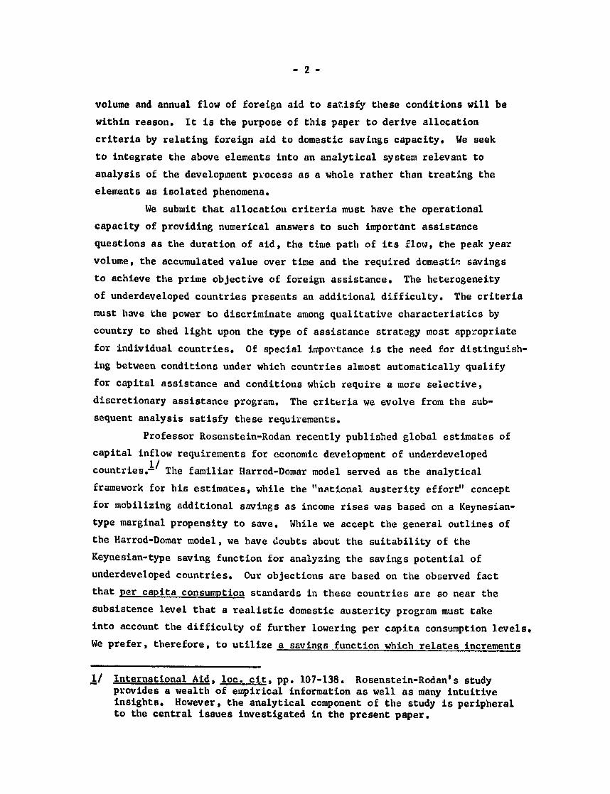
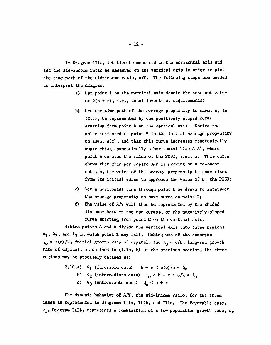