ood insecurity in sub-saharan africa: new estimates...
TRANSCRIPT

Food Insecurity in Sub-Saharan Africa
New Estimates from Household Expenditure Surveys
Lisa C. SmithHarold AldermanDede Aduayom
RESEARCHREPORT 146INTERNATIONAL FOOD POLICY RESEARCH INSTITUTEWASHINGTON, D.C.

Copyright © 2006 International Food Policy Research Institute. All rights reserved.Sections of this material may be reproduced for personal and not-for-profit usewithout the express written permission of but with acknowledgment to IFPRI. Toreproduce the material contained herein for profit or commercial use requires expresswritten permission. To obtain permission, contact the Communications Division<[email protected]>.
International Food Policy Research Institute2033 K Street, N.W.Washington, D.C. 20006-1002U.S.A.Telephone +1-202-862-5600www.ifpri.org
Library of Congress Cataloging-in-Publication Data
Smith, Lisa C.Food insecurity in sub-Saharan Africa : new estimates from household
expenditure surveys / Lisa C. Smith, Harold Alderman, Dede Aduayom.p. cm. — (Research report ; 146)
Includes bibliographical references.ISBN 0-89629-150-2 (alk. paper)1. Food supply—Africa, Sub-Saharan. I. Alderman, Harold, 1948–
II. Aduayom, Dede. III. Title. IV. Series: Research report (International Food Policy Research Institute) ; 146.HD9017.A3572S65 2006338.1′967—dc22 2006008740

Contents
List of Tables iv
List of Figures vi
List of Boxes vii
Foreword viii
Acknowledgments ix
Summary x
1 Introduction 1
2 Conceptual and Empirical Basis for Measures of Food Insecurity 4
3 Data and Methods 17
4 Estimates of Food Insecurity 31
5 Comparison with FAO Estimates and Related Measures 44
6 Evidence on Cross-Country Comparability and Other Reliability Issues 63
7 Conclusion 69
Appendix A: Data Sets Not Included in the Study and Reasons Why 75
Appendix B: Data Collection and Processing by Country 77
Appendix C: Standard Errors for Estimates of Food Security Measures 98
Appendix D: Country Food Security Profiles 100
Appendix E: Methods of Estimating Global and Regional Food Energy Deficiency Prevalences when Data Are Not Available for All Countries 112
Appendix F: Differences in Food Security Measures across Total Expenditure Quintiles when Quintiles Are Not Based on Predicted Expenditures 114
References 116
iii
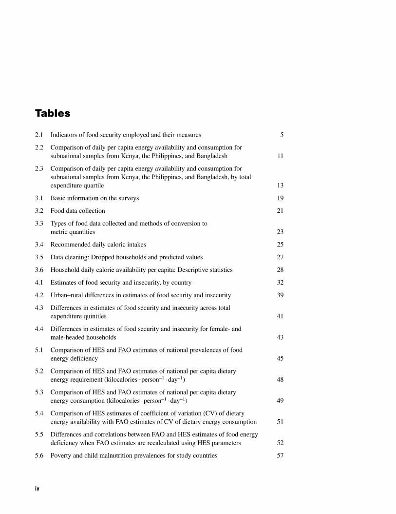
Tables
2.1 Indicators of food security employed and their measures 5
2.2 Comparison of daily per capita energy availability and consumption for subnational samples from Kenya, the Philippines, and Bangladesh 11
2.3 Comparison of daily per capita energy availability and consumption for subnational samples from Kenya, the Philippines, and Bangladesh, by totalexpenditure quartile 13
3.1 Basic information on the surveys 19
3.2 Food data collection 21
3.3 Types of food data collected and methods of conversion to metric quantities 23
3.4 Recommended daily caloric intakes 25
3.5 Data cleaning: Dropped households and predicted values 27
3.6 Household daily calorie availability per capita: Descriptive statistics 28
4.1 Estimates of food security and insecurity, by country 32
4.2 Urban–rural differences in estimates of food security and insecurity 39
4.3 Differences in estimates of food security and insecurity across total expenditure quintiles 41
4.4 Differences in estimates of food security and insecurity for female- and male-headed households 43
5.1 Comparison of HES and FAO estimates of national prevalences of food energy deficiency 45
5.2 Comparison of HES and FAO estimates of national per capita dietary energy requirement (kilocalories ⋅ person–1 ⋅ day–1) 48
5.3 Comparison of HES and FAO estimates of national per capita dietary energy consumption (kilocalories ⋅ person–1 ⋅ day–1) 49
5.4 Comparison of HES estimates of coefficient of variation (CV) of dietary energy availability with FAO estimates of CV of dietary energy consumption 51
5.5 Differences and correlations between FAO and HES estimates of food energydeficiency when FAO estimates are recalculated using HES parameters 52
5.6 Poverty and child malnutrition prevalences for study countries 57
iv

5.7 Correlations between estimates of food energy deficiency and poverty and child malnutrition 59
5.8 Expert opinion survey: Respondent rankings 61
5.9 Expert opinion survey: Comparison of country rankings with those derived from FAO and HES estimates of food energy deficiency 62
5.10 Expert opinion survey: Tests of association of country rankings with those derived from FAO and HES estimates of food energy deficiency 62
6.1 Food security indicators, by data collection method 64
6.2 Comparison of national prevalences of food energy deficiency estimated with energy requirements applied at the household and national levels 66
6.3 Prevalences of food energy deficiency at alternative coefficients of variation of dietary energy availability per capita 67
A.1 Data sets not included in the study and reasons why 75
C.1 Standard errors for estimates of food energy availability 98
C.2 Standard errors for estimates of food energy deficiency 98
C.3 Standard errors for estimates of household dietary diversity 99
C.4 Standard errors for estimates of the prevalence of low diet diversity 99
D.1 Food security profile for Burundi, 1998 100
D.2 Food security profile for Ethiopia, 1999 101
D.3 Food security profile for Ghana, 1998 102
D.4 Food security profile for Guinea, 1994 103
D.5 Food security profile for Kenya, 1997 104
D.6 Food security profile for Malawi, 1997 105
D.7 Food security profile for Mozambique, 1996 106
D.8 Food security profile for Rwanda, 2000 107
D.9 Food security profile for Senegal, 2001 108
D.10 Food security profile for Tanzania, 2000 109
D.11 Food security profile for Uganda, 1999 110
D.12 Food security profile for Zambia, 1996 111
F.1 Differences in food security measures across total expenditure quintiles when quintiles are not based on predicted expenditures 114
TABLES v
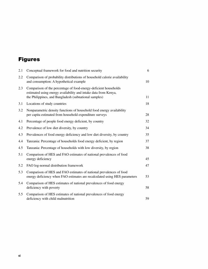
Figures
2.1 Conceptual framework for food and nutrition security 6
2.2 Comparison of probability distributions of household calorie availability and consumption: A hypothetical example 10
2.3 Comparison of the percentage of food-energy-deficient households estimated using energy availability and intake data from Kenya, the Philippines, and Bangladesh (subnational samples) 11
3.1 Locations of study countries 18
3.2 Nonparametric density functions of household food energy availability per capita estimated from household expenditure surveys 28
4.1 Percentage of people food energy deficient, by country 32
4.2 Prevalence of low diet diversity, by country 34
4.3 Prevalences of food energy deficiency and low diet diversity, by country 35
4.4 Tanzania: Percentage of households food energy deficient, by region 37
4.5 Tanzania: Percentage of households with low diversity, by region 38
5.1 Comparison of HES and FAO estimates of national prevalences of food energy deficiency 45
5.2 FAO log-normal distribution framework 47
5.3 Comparison of HES and FAO estimates of national prevalences of food energy deficiency when FAO estimates are recalculated using HES parameters 53
5.4 Comparison of HES estimates of national prevalences of food energy deficiency with poverty 58
5.5 Comparison of HES estimates of national prevalences of food energy deficiency with child malnutrition 59
vi
Boxes
5.1 Expert Opinion Survey on Food Insecurity in Study Countries: Questionnaire 60
vii

Foreword
Reducing food insecurity in the developing world continues to be a major public policy
challenge, and one that is complicated by lack of information on the location, severity,
and causes of food insecurity. Such information is needed to properly target assistance,
evaluate whether progress is achieved, and develop appropriate interventions to help those in
need. This research report explores a new method of measuring food insecurity using food
data collected as part of household expenditure surveys. Such surveys are routinely under-
taken by numerous national governments throughout the developing world, but in the past the
resulting food data remained largely unexploited for the purposes of measuring food insecurity.
Using data from 12 Sub-Saharan African countries, this innovative and scholarly research
by Lisa Smith, Harold Alderman, and Dede Aduayom demonstrates the value of such data for
generating estimates of both diet quantity indicators, such as the share of populations that are
food-energy deficient, and diet quality indicators, such as diet diversity.
While the approach does not permit an annual update of the food security situation due to
the time-consuming nature of household surveys, the results indicate that household expendi-
ture surveys are a rich source of data for improving food security measurement. The approach
facilitates an improved understanding of benchmarking and progress toward the United Na-
tions’ Millennium Development Goal of halving the proportion of people suffering from
hunger by 2015, and similarly of the much-preferred World Food Summit Goal of actually
cutting the absolute number of undernourished people in half by that time. We hope that
updates to these household-based data sources are done, at minimum, on a five-year basis to
enrich the understanding of progress in food security, or the lack thereof.
Joachim von Braun
Director General, IFPRI
viii

Acknowledgments
Funding for this research has been generously provided by the Australian Agency forInternational Development, the Canadian International Development Agency, the De-partment for International Development of the United Kingdom, the United States
Agency for International Development’s Presidential Initiative to End Hunger in Africa, theUnited States Department of Agriculture, and the World Bank.
The Africa Household Survey Databank of the World Bank, which facilitated access tomany of the data sets, and especially the ready assistance of Pascal Heus and ChristopherRockmore are gratefully acknowledged.
The following government statistical services administered the surveys and compiled thedata sets used in this study:• Institut de Statistiques et d’Etudes Economiques du Burundi• Central Statistical Authority of Ethiopia• Ghana Statistical Service• Direction Nationale de la Statistique, Republique de Guinee• Central Bureau of Statistics of Kenya• National Statistical Office of Malawi• Instituto Nacional de Estatistica de Mozambique• Direction de la Statistique de Rwanda• Direction de la Prévision et de la Statistique de Senegal• National Bureau of Statistics of Tanzania• Uganda Bureau of Statistics• Central Statistical Office of Zambia
We thank the staff members of these organizations who helped to answer our questions andfind additional data needed to undertake the analysis.
We would like to especially acknowledge Lawrence Haddad for his role in instigating thisresearch program, his continual strong support throughout, and his technical contributions.
Elizabeth Byron, Timothy Frankenberger, Joachim Von Braun, Doris Wiesmann, twoanonymous referees, and the Socio-Economic Statistics and Analysis Service of the StatisticsDivision of FAO gave valuable comments on the manuscript. We also appreciate the com-ments and feedback of participants at presentations made at IFPRI, FAO, and the FIVIMSInternational Scientific Conference on Food Deprivation and Undernutrition in June 2002.
This research required a great deal of data processing, computer programming, investiga-tive inquiry, and travel to many of the study countries. Doris Wiesmann, Ibrahima Wane, AliSubandoro, Arif Rashid, Ellen Payongayong, Aida Ndaiye, Smita Ghosh, Elizabeth Byron,and Joshua Ariga are thanked for their assistance with these tasks.
The findings, interpretations, and conclusions expressed in this report are entirely those ofthe authors. They do not necessarily represent the view of the World Bank, its executive di-rectors, or the countries they represent, or of IFPRI and its supporting organizations.
ix
Summary
Hunger is a pervasive problem in developing countries, undermining people’s health,productivity, and often their very survival. Therefore, much of the developmentagenda focuses on directing scarce resources to providing food to people in need or
enabling them to acquire it themselves. The foundation for doing so is a reliable informationbase on food insecurity—that is, access by people to food—which is the most immediatecause of hunger. Such information is fundamental to effectively targeting assistance, evaluat-ing progress, and developing interventions. Its need is now more urgent than ever as effortsare stepped up to meet the Millennium Development Goal (MDG) of halving the proportionof people who suffer from hunger by 2015. Yet arriving at an accurate measure of food inse-curity that is comparable both within and across countries remains a challenge. The indicatormost widely employed by policymakers is the measure of “undernourishment,” or the per-centage of a country’s population that does not consume sufficient dietary energy, by the Foodand Agriculture Organization of the United Nations (FAO). This method is based on a coun-try’s food supplies rather than directly on data representing peoples’ access to food. Given alack of data collected at the household or individual level in national surveys, this is the onlyfeasible method at present, though its reliability for policymaking and program planning hasbeen the subject of considerable debate.
This report introduces new estimates of food insecurity based on food acquisition datacollected directly from households as part of national household expenditure surveys (HESs)conducted in 12 Sub-Saharan African countries. The report has three objectives: (1) to explorethe extent and location of food insecurity across and within the countries; (2) to investigatethe scientific merit of using the food data collected in HESs to measure food insecurity; and(3) to compare food insecurity estimates generated using HES data with those reported byFAO and explore the reasons for differences between the two. The overall purpose is to in-vestigate how the data collected in HESs can be used to improve the accuracy of FAO’s esti-mates, which are being used to monitor the MDG hunger goal. The study is based on both dietquantity and diet quality indicators of food insecurity. The two main indicators of focus are theshare of people consuming insufficient dietary energy, or the prevalence of “food energy de-ficiency” and the share of households with low diet diversity. The study finds these to be validindicators of food insecurity and to be reasonably reliably measured. They are also comparableacross the study countries despite differing methods of data collection.
This report confirms that food insecurity is a major problem in Sub-Saharan Africa. Theprevalences of food energy deficiency among the study countries range from 37 percent(Uganda) to 76 percent (Ethiopia). Problems of diet quality associated with the region’s highrates of micronutrient deficiencies are found to be widespread. Notably, there is no strong as-sociation between the diet quantity and diet quality measures. If both of these aspects of foodinsecurity are taken into account, country rankings differ substantially from results consideringdiet quantity alone, which is the convention.
HESs offer a rich lens through which to examine food insecurity within countries as well.The socioeconomic characteristics examined here—region of residence, urban or rural resi-
x

dence, economic status, and female- or male-headed household—are only a few of particularinterest to policymakers. The study countries display wide variation in the characteristics, withthe only consistent patterns emerging being that male-headed households in eastern and south-ern Africa and urbanites have a clear advantage when it comes to diet quality. As expected,income has a potent bearing on food insecurity.
The study identified strong differences between HES and FAO estimates of food energydeficiency for the 12 study countries, resulting in significantly different pictures of the mag-nitude of food insecurity in the countries and country rankings. The main source of the diver-gences lies in differences in the national-level parameters used to generate the FAO estimates(mean energy availability, energy requirement, and distribution across households) rather thanin the method itself. The lower requirement used explains why FAO estimates are almostuniformly lower than those reported here. Nevertheless, the most important factor behind thedivergence between the FAO and HES estimates is not found there but in the differences inthe underlying estimates of national energy availability.
HES estimates of food energy deficiency are found to be more strongly associated withother MDG indicators of poverty and hunger than are the FAO estimates. The correlation be-tween HES country rankings and poverty is 3.6 times higher than that for the FAO estimates.The same correlation for estimates of child malnutrition is 1.7 times higher. The HES esti-mates are also more consistent with country rankings based on a survey of expert opinion.These findings provide empirical support that HES data are a useful source of information forimproving the accuracy of FAO estimates of food insecurity.
The main advantage of using HES data for measuring food insecurity is that they are asource of multiple, policy-relevant, and reasonably reliable measures. They allow multilevelmonitoring and evaluation, including that of within-country and national food insecurity and,given data from a sufficient number of countries, of regional and developing-world food in-security as well. Their main disadvantage is that data are not collected for all countries reg-ularly, partly because of the financial resources and skill levels required for data collection,processing, and analysis. Creating a database of cross-country comparable estimates of foodinsecurity based soundly on household-level data, while currently not feasible, is fast becom-ing a reality as the surge in the collection of HESs that began in the 1990s continues.
Meanwhile, HES data can be used to improve the accuracy of the FAO’s estimates in anumber of ways: first, they can improve estimates of national food supplies; second, they canimprove the accuracy of estimates of the distribution of dietary energy across countries’ pop-ulations and increase the number of countries for which they are available; and, finally, HES-derived estimates of food energy deficiency can continue to serve as a reference for compari-son and validation. The above endeavors require that this report’s analysis be extended to theother developing regions, providing the essential data for (1) improving estimates of energyavailabilities and their distribution and (2) generating regional and developing-world estimatesof food insecurity using FAO or alternative methods. Additionally, basic research is needed toresolve outstanding reliability issues in the estimation of food energy deficiency and poor dietquality from HESs. Finally, because many HESs are not undertaken with the intention of cal-culating measures of food insecurity, they often do not contain the appropriate data for doingso. To remedy this problem, guidelines containing best practices for collecting and processingHES food data are needed.
SUMMARY xi

C H A P T E R 1
Introduction
Food is the most basic of human needs for survival, health, and productivity. It is thusthe foundation for human and economic development. As is now well known, enoughfood and much more is produced to meet the needs of all people in the world today.
Hunger nevertheless remains a pervasive problem in developing countries, and much of thedevelopment agenda must focus scarce resources on either providing food to people in needor enabling them to acquire it themselves. The foundation for doing so is a reliable informa-tion base on “food insecurity”—the most immediate cause of hunger1—which is needed foranswering some essential questions:• Where are the world’s hungry?• How many people are hungry?• How is hunger changing over time?• What are the causes of hunger?
In turn, the answers to these questions are essential for targeting assistance, evaluatingwhether progress is being achieved, and developing appropriate policies and programs forhelping people. Knowing these answers is urgent given the undoubtedly large numbers ofpeople affected, including 148 million developing country children under 5 who are stunted.It has become even more urgent as efforts are stepped up to meet the Millennium Develop-ment Goal (MDG) of halving the proportion of people who suffer from hunger by 2015.
Although there is now general agreement on what food insecurity is—that is, a phe-nomenon of access by people to food rather than only the availability of food in a country—arriving at an accurate measure of it that is comparable both within and across countriesremains a challenge. Currently existing methods of measuring food insecurity suffer from anumber of limitations.
The methods most widely employed for cross-country comparisons are based on nationalaggregate data on food availability or income rather than directly on data representing peo-ples’ access to food. These are at present the only feasible methods because of a lack of suffi-cient food data collected at the household or individual level in nationally representative sur-veys. The method most widely cited and employed by policymakers is the United NationsFood and Agriculture Organization (FAO) measure of “undernourishment,” a measure ofthe percentage of countries’ populations that does not have access to sufficient dietary energy
1It is important to note that “hunger” and “food insecurity” are distinct concepts. Whereas food insecurity refersto lack of access to food, hunger is “an uneasy sensation, exhausted condition, caused by want of food” (OxfordEnglish Dictionary).
1
(Naiken 2003). It is based on national foodsupply data. The United States Departmentof Agriculture (USDA) reports estimatesof the same measure based on countries’ na-tional incomes along with food supplies(Shapouri and Rosen 1999; Senauer and Sur2001).
Although these methods yield estimatesthat are useful advocacy tools for reduc-ing hunger and may capture broad regionaldifferences and trends, their reliability forpolicymaking and program planning, par-ticularly that of FAO’s country estimates,has been the subject of considerable debate(Naiken [cited in Smith 1998b]; Smith1998a; Svedberg 2000; Gabbert and Wei-kard 2001; Haddad 2001; Aduayom andSmith 2003; Broca 2003; David 2003;Senauer 2003; Svedberg 2003). There arelarge discrepancies between the FAO andUSDA estimates of the prevalence of foodenergy deficiency at even the level of thedeveloping-country regions. For example,the FAO estimate of the prevalence for Sub-Saharan Africa was 34 percent in 1997–1999 (FAO 2001). That reported by USDAfor the same period was 50 percent (Sha-pouri and Rosen 1999). The difference in theestimates for Latin America and the Carib-bean is even higher, with FAO reporting11 percent and USDA reporting 40 per-cent. These discrepancies send conflictingmessages to policymakers hoping to effi-ciently target resources toward reducing foodinsecurity.
For the practical purposes of food se-curity policy decisionmaking, the methodsbased on aggregate food availabilities andincomes have three further limitations:(1) they cannot be used for determining thelocation of food insecurity within countries;2
(2) they have limited use for understanding
the causes of food insecurity; and (3) theyfocus only on diet quantity to the exclusionof other important aspects of food security,such as diet quality and vulnerability (Smith2003).
Two alternative measures that are basedon household survey data are considered tobe reliable but do not measure valid indica-tors of food insecurity. Height and weightdata collected using anthropometric methodsare the basis for a measure of “undernutri-tion,” which is influenced not only by foodconsumption but also by health status (Shetty2003). Poverty or “livelihood insecurity”measures capture people’s ability to satisfya number of different basic needs, amongwhich tight trade-offs may be faced, not justfood (Frankenberger et al. 1997).
Two final methods of measuring foodsecurity are considered to be reliable andbased on valid indicators but suffer fromsome practical constraints. The first mea-sures nutrient adequacy from data collectedon individual or household food intake, usu-ally over the previous 24 hours. This methodis far too costly to implement on a nationalscale for most countries (Ferro-Luzzi 2003;Swindale and Ohri-Vachaspati 2004). Thesecond uses qualitative measures to capturepeople’s own perceptions of the extent towhich they suffer from hunger. Althoughmore research is needed, this method haslimited usefulness for cross-country com-parisons because surveys must be adaptedto local circumstances (Kennedy 2003).
The purpose of this report is to introducenew estimates of food insecurity based onfood data collected directly from house-holds as part of national household expen-diture surveys (HESs). In these surveys,households are asked to report the quantitiesof or expenditures on foods they acquired in
2 CHAPTER 1
2With respect specifically to the FAO measure, food supply data are not used to estimate subnational differencesin food availability and deficiency because, as stated in Naiken (2003), “it is not possible to disaggregate the na-tional estimate by subnational areas as the food balance sheet approach is not applicable at the subnational level”(page 25). Presumably this is because the approach relies on imports and exports of food to determine how muchfood is available in a country, and only production data are collected for subnational regions.
the recent past, commonly the last 1 or 2weeks. They are asked about their food pur-chases, the food they consume from theirown fields or gardens, and, usually, foodreceived in kind as well. The data, whencomplemented by metric weights of foodreported in local units of measure or metricfood prices, allow estimation of quantitiesof food acquired by households. These canthen be used to calculate a number of mea-sures of food security and insecurity at na-tional and subnational levels. The data allowdetermination of whether a household hasacquired sufficient food to meet its mem-bers’ energy requirements in addition tocalculation of measures of diet quality, anequally important aspect of food security.
Over the 1990s and continuing into thepresent, there has been a surge in the col-lection of national HESs, whether by gov-ernment statistical services or through theWorld Bank’s Living Standards Measure-ment Survey program or its associated re-gional programs. HESs are becoming moreand more routinely collected and used aspart of the information base for policy de-cisions by governments and internationaldevelopment agencies. Thus, creating across-country comparable global food se-curity database founded on them, althoughcurrently not feasible, is fast becoming areality.
The report focuses on the developingcountry region that is considered to have themost severe food insecurity, Sub-SaharanAfrica. Many countries in the region are noteven able to meet the food needs of theirpopulations at the aggregate, national level,much less ensure that sufficient food reachesall people (Smith et al. 1999). One-quarterof all preschool children in the region wereunderweight, and one-third stunted, in 2000(ACC/SCN 2004). Poor diet quality is a se-rious problem. Forty-three percent of theregion’s people, including the same per-centage of school-age children, suffer fromiodine deficiency, the primary cause of pre-ventable mental retardation in children.About one-third of all preschool children
have a dietary deficiency of vitamin A, anessential micronutrient for normal function-ing of the visual system, growth and devel-opment, immune function, and reproduction(ACC/SCN 2004). Further, the populationaffected by goiter as a result of iodine defi-ciency is 20 percent, the highest in the de-veloping world (ACC/SCN 2000).
The report has three objectives. The firstis to explore the location and extent of foodinsecurity across and within 12 Sub-SaharanAfrican countries with HESs conducted inthe 1990s. The countries are Burundi,Ethiopia, Ghana, Guinea, Kenya, Malawi,Mozambique, Rwanda, Senegal, Tanzania,Uganda, and Zambia. The second is to ex-plore the scientific merit of using HESs tomeasure food insecurity, taking a look at thevalidity of the measures that can be esti-mated, the reliability of the methods fordoing so, and international comparability.The third is to compare the food energy de-ficiency estimates generated from HES datawith FAO’s undernourishment estimatesand begin to explore the reasons for any dif-ferences between the two. The ultimate aimis to look for ways to improve the accuracyof FAO’s estimates, which are being used tomonitor progress toward reaching the Mil-lennium Development Goal on hunger.
The report is organized as follows.Chapter 2 describes the indicators of foodsecurity used in this study and discussesmeasurement issues. Chapter 3 presents thedata sets employed and lays out the method-ology for calculating the measures. Chapter4 reports the estimates of food insecurity,comparing population groups both acrossand within countries. In Chapter 5, the esti-mates of national food energy deficiencyprevalence are compared with those re-ported by FAO, and some reasons for thedifferences are explored. Chapter 6 presentsevidence on comparability of the estimatesacross countries and some other reliabilityissues. Chapter 7 concludes with a summaryof the findings and a discussion of howHESs can help improve the reliability ofglobal food insecurity estimates.
INTRODUCTION 3
C H A P T E R 2
Conceptual and Empirical Basis forMeasures of Food Insecurity
This chapter first describes the indicators of food security used in the report and theirmeasures. Following this, the conceptual validity of the indicators, that is, how wellthey conform to the definition of food security given, is discussed. Next, the reliability
of the measures is addressed. Are we accurately capturing the measures with the data and themethod of calculation used? Finally the issue of comparability across countries of the mea-sures is taken up.
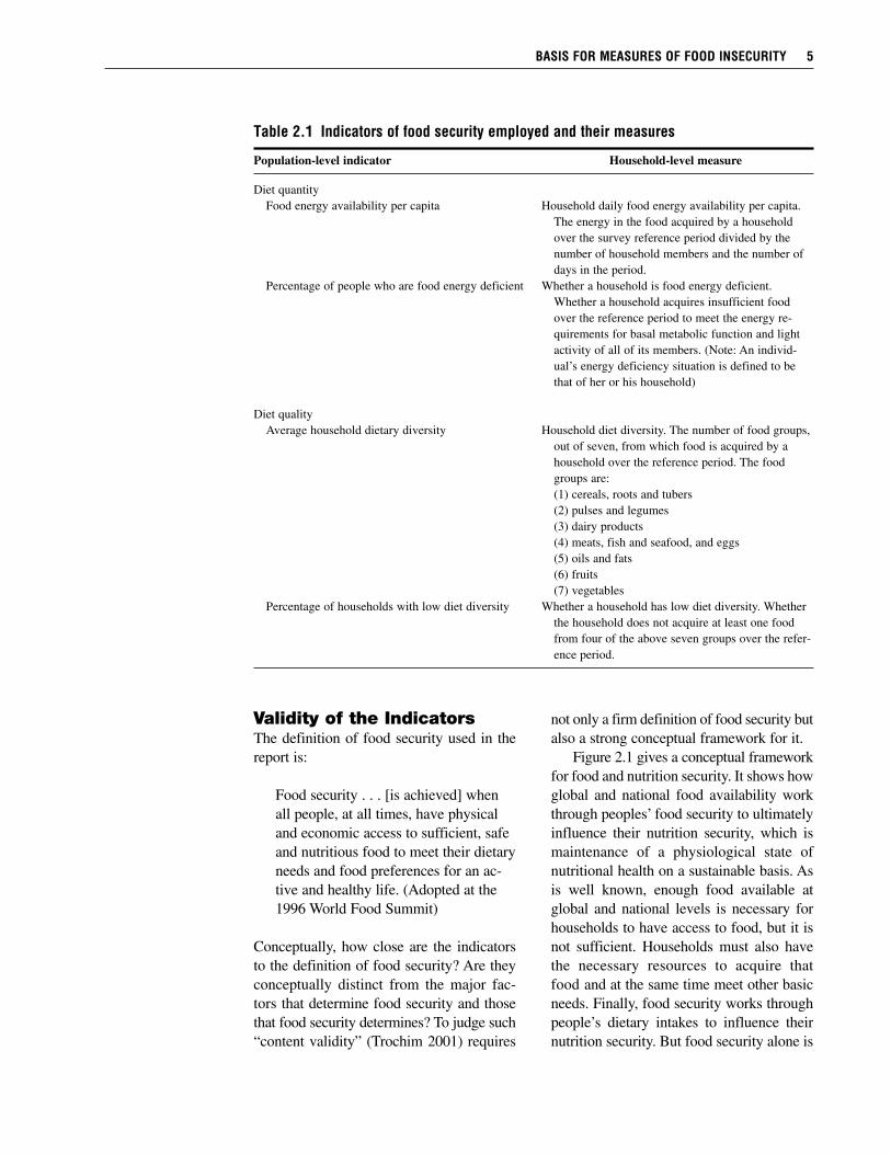
Food Security Indicators and Their MeasuresThe four indicators of food security (and insecurity) employed in this report, along with a de-scription of how they are measured at the household level, are listed in Table 2.1.
The first two are indicators of diet quantity, the amount of food eaten by people. The firstis average household food energy availability per person. It is measured as the amount of en-ergy in the food acquired by the household over the survey reference period divided by thenumber of household members and days in the period. The data collected from households inHESs are either (1) expenditures on each food or (2) quantities acquired of them, which areoften reported in nonmetric or “local” units of measure, for example, bunches or cans. The firstessential step in calculating this measure is to convert the data to metric quantities (grams orkilograms). To do this, reported expenditures on each food are divided by the food’s metricprice; reported quantities in local units of measure are multiplied by the food’s metric weight.The energy content of the food acquired can then be determined using food composition tables.
The second diet quantity indicator is the percentage of people in a population group whodo not consume sufficient dietary energy. It is measured by determining whether a person livesin a household that acquires sufficient food over the survey reference period to meet the di-etary energy requirement of all of its members. The total energy in the food that the householdacquires is compared to the sum of the daily energy requirements of each of its members. Therequirements employed are for basal metabolic function (a state of complete rest) and light ac-tivity, such as sitting and standing.
The next two indicators, household diet diversity and the percentage of households with“low diet diversity,” are indicators of diet quality. Diet diversity indicates how varied the fooda household consumes is. Based on the quantity or expenditure data collected from households,it is calculated by counting the number of food groups, out of seven (see Table 2.1), fromwhich food is acquired over the survey reference period. The percentage of households withlow diet diversity is measured by determining whether a household fails to acquire at least onefood from four of the seven groups over the reference period.
4
Validity of the IndicatorsThe definition of food security used in thereport is:
Food security . . . [is achieved] whenall people, at all times, have physicaland economic access to sufficient, safeand nutritious food to meet their dietaryneeds and food preferences for an ac-tive and healthy life. (Adopted at the1996 World Food Summit)
Conceptually, how close are the indicatorsto the definition of food security? Are theyconceptually distinct from the major fac-tors that determine food security and thosethat food security determines? To judge such“content validity” (Trochim 2001) requires
not only a firm definition of food security butalso a strong conceptual framework for it.
Figure 2.1 gives a conceptual frameworkfor food and nutrition security. It shows howglobal and national food availability workthrough peoples’ food security to ultimatelyinfluence their nutrition security, which ismaintenance of a physiological state ofnutritional health on a sustainable basis. Asis well known, enough food available atglobal and national levels is necessary forhouseholds to have access to food, but it isnot sufficient. Households must also havethe necessary resources to acquire thatfood and at the same time meet other basicneeds. Finally, food security works throughpeople’s dietary intakes to influence theirnutrition security. But food security alone is
BASIS FOR MEASURES OF FOOD INSECURITY 5
Table 2.1 Indicators of food security employed and their measures
Population-level indicator Household-level measure
Diet quantityFood energy availability per capita Household daily food energy availability per capita.
The energy in the food acquired by a householdover the survey reference period divided by thenumber of household members and the number ofdays in the period.
Percentage of people who are food energy deficient Whether a household is food energy deficient. Whether a household acquires insufficient foodover the reference period to meet the energy re-quirements for basal metabolic function and lightactivity of all of its members. (Note: An individ-ual’s energy deficiency situation is defined to bethat of her or his household)
Diet qualityAverage household dietary diversity Household diet diversity. The number of food groups,
out of seven, from which food is acquired by ahousehold over the reference period. The foodgroups are:(1) cereals, roots and tubers(2) pulses and legumes(3) dairy products(4) meats, fish and seafood, and eggs(5) oils and fats(6) fruits(7) vegetables
Percentage of households with low diet diversity Whether a household has low diet diversity. Whether the household does not acquire at least one foodfrom four of the above seven groups over the refer-ence period.
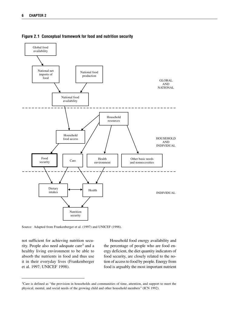
not sufficient for achieving nutrition secu-rity. People also need adequate care3 and ahealthy living environment to be able toabsorb the nutrients in food and thus useit in their everyday lives (Frankenbergeret al. 1997; UNICEF 1998).
Household food energy availability andthe percentage of people who are food en-ergy deficient, the diet quantity indicators offood security, are closely related to the no-tion of access to food by people. Energy fromfood is arguably the most important nutrient
6 CHAPTER 2
3Care is defined as “the provision in households and communities of time, attention, and support to meet thephysical, mental, and social needs of the growing child and other household members” (ICN 1992).
Figure 2.1 Conceptual framework for food and nutrition security
Source: Adapted from Frankenberger et al. (1997) and UNICEF (1998).
Global foodavailability
National foodproduction
National netimports of
food
National foodavailability
Householdresources
Householdfood access
Foodsecurity Care Health
environmentOther basic needsand nonnecessities
Dietaryintakes
Nutritionsecurity
HealthINDIVIDUAL
HOUSEHOLDAND
INDIVIDUAL
GLOBALAND
NATIONAL

for survival, physical activity, and health,and households are the units through whichpeople generally access food. The indicatorspertain to the amount and sufficiency of en-ergy in the food that is immediately avail-able to households for consumption, whichis a clear indication of their ability to accesssufficient food.
Importantly, the indicators are clearlydistinct from indicators of related concepts.They are obviously distinct from national(or even local) food availability, which is adeterminant of food security. They are alsodistinct from indicators of household re-source holdings, such as poverty, whichcaptures households’ abilities to meet all oftheir needs, not just food. Finally, they aredistinct from nutrition security, which foodsecurity determines, but not alone. Thus,from a conceptual standpoint, the two indi-cators of diet quantity derived from HESsare valid indicators of food security.
In regard to the diet quality indicators—household diet diversity and the percentageof households with low diet diversity—it iswell known that energy is not the only nu-trient people need to lead active, healthylives. It is quite possible for a person to meether or his energy requirement but to be pre-vented from achieving full physical and in-tellectual potential as a result of deficienciesof other nutrients, specifically protein andmicronutrients such as iron, vitamin A, andiodine (Welch 2004). It is increasingly rec-ognized that inadequate diet quality, ratherthan sufficient energy consumption, is be-coming the main dietary constraint facingpoor populations (Ruel et al. 2003; Graham,Welch, and Bouis 2004). Further, a numberof studies have documented that improveddiet quality as indicated by a more varied dietis associated with improved birth weight andchild anthropometric status and with reducedmortality (Ruel 2002, 2003). Thus, it is im-
portant that indicators of the nutritional qual-ity of the food people eat be included in anyanalysis of food security. Like the indicatorsof diet quantity, the diet quality indicatorsare conceptually distinct from their determi-nants (food availability and household re-sources) and outcomes (nutrition security).
In sum, the food security indicators em-ployed in this report have strong concep-tual validity. They cover important aspectsof the definition—access, sufficiency, andquality—and capture these aspects well.They do not fully conform to the definition,however, for the following reasons. First, acomplete picture of the state of food secu-rity should cover an important aspect of itsdefinition that the four indicators do notaddress: vulnerability to food deprivationin the future (Maxwell and Frankenberger1992). The indicators do not indicatewhether people have access to food at alltimes. Second, the definition of food secu-rity stresses that all people have access tofood. Yet the food data collected in house-hold expenditure surveys indicate access tofood of households, not individuals withinthem.4 It is now well known that intra-household food distribution is not alwayssuch that all household members receive thefood that they need even if sufficient foodis available at the household level (Haddadand Kanbur 1990). Finally, the indicator setdoes not address issues of food safety andfood preferences.
Reliability of the MeasuresOne of the main advantages of using house-hold expenditure surveys (HESs) to measurefood security is that the source of the fooddata collected is the people (adult women ormen) living in surveyed households. The in-formation comes directly from the location inwhich behavior regarding food consumption
BASIS FOR MEASURES OF FOOD INSECURITY 7
4Vasdekis, Stylianou, and Naska (2001) propose a methodology to estimate age- and gender-specific food avail-ability using the household-level data collected in household expenditure surveys that may be useful for futureanalyses.

takes place and from the people consumingthe food. Further, compared to data on othermeasures of households’ resource holdings,such as income and assets, food expendi-tures data are not especially sensitive; peo-ple generally have little incentive to mis-report how much food they acquire over ashort period of time.5 Although they may beemployed to measure food insecurity forbroad geographic areas, the food data col-lected reflect the food acquired by a house-hold rather than by groups of households inthese broader areas, for example, countriesor regions within them. Systematic, scien-tific sampling is the norm, yielding samplesthat are, for the most part, nationally rep-resentative.6 Although, as discussed below,many types of error can affect estimates offood security, it is these traits that give con-fidence that gross errors in estimates of foodinsecurity derived from HESs are avoided.
Quantities of Food AcquiredAll four measures described above are basedon the data collected on households’ acqui-sition of food. The most common methodof data collection is the personal interviewin which an enumerator asks one or morehousehold members to recall quantities ac-quired and/or expenditures made over the“reference period” for food data collection.This period is the total amount of time forwhich food data are collected, commonly 1or 2 weeks. The diary method may be em-ployed for households with a literate mem-ber. To take into account seasonal variationin food consumption associated with theagricultural cycle, data may be collectedeither in multiple rounds throughout a yearor in one-time interviews conducted ran-
domly across groups of households through-out a year (see more on the implications ofthis choice below).
A number of nonsampling errors in themeasurement of household food acquisitionarise during the collection and preparationof HES data. The first is that data collectionis plagued by the typical reporting biasesand recording errors faced by all householdsurveys. Respondents may become tired ordespondent because they are overwhelmedby the length of the survey or the number ofitems covered. They may change their nor-mal food acquisition behavior as a result ofbeing included in the survey (“conditioningeffects”) (Deaton and Grosh 2000). Further,the enumerator may cause the respondent toreport incorrectly by asking vague or “lead-ing” questions. He or she may also recordthe respondent’s response to questions in-correctly on the questionnaire or with hand-writing that cannot be read by data entry op-erators. And of course, data entry operatorsmay enter the data incorrectly.
Two important types of systematic biasmay arise because respondents have diffi-culty remembering the food their householdacquired over the survey recall period. Thefirst, known as “recall bias,” is that respon-dents may have difficulty remembering theirfood acquisition over the period itself, re-sulting in a downward bias. The second isbias as a result of “telescoping,” where a re-spondent may include events that occurredbefore the recall period, thus inflating esti-mates of household food acquisition. Theshorter the recall period, the more likely istelescoping; the longer the recall period, themore likely is recall bias. In the specific caseof food acquisitions, which are of high fre-
8 CHAPTER 2
5There are exceptions, however. For example, households may falsely report a larger than true expenditure on ahigh-prestige food (such as meat) or understate foods acquired in the belief that food aid may be forthcoming fol-lowing the survey. These kinds of misreporting are likely to be less of a problem in household expenditure sur-veys, in which data are collected on a large number of subjects, than in specialized household food consumptionsurveys.
6Population groups that are left out of the censuses that serve as sampling frames are migrants, homeless people,and people living in institutions. Sometimes people living in areas with violence related to conflict or that are other-wise physically inaccessible may also be left out.

quency and small size compared to nonfoodacquisitions, recall bias is thought to bemore of a problem than telescoping (Deatonand Grosh 2000).
Another area where errors can arise isin the conversion of the data collected onexpenditures or quantities to their metricequivalents. If expenditures are collected,they must be divided by metric prices offoods. Obviously, the prices used shouldrepresent those faced by the household atthe time of the purchase or, in the case ofa home-produced food, if it were to buy orsell the food. But this information is notusually collected in HESs, and estimatedprices must be used as proxies. They maybe estimated as median unit values fromhouseholds located in the immediate vicin-ity or even the administrative region, or theymay be collected in a price survey adminis-tered at the community level or at a broaderregional level. However, in the case of pricesurveys, it may be difficult for a surveyteam to replicate the kind of transaction thata household itself would engage in. Pricesfaced may vary even among householdsthat purchase from the same source dueto different negotiating abilities or personalconnections. Further, richer householdsmay buy higher-quality products that havehigher prices (Deaton and Grosh 2000).
Data collected on the physical quantitiesof foods, rather than expenditures, may bemore accurate if foods are weighed usingscales on the spot or, for packaged foods,the weight is recorded directly from con-tainers in which they are acquired. However,this technique is rare because it is so timeconsuming. Further, if the acquired food hasalready been consumed, it is no longer pos-sible to physically observe and measure it.In most surveys, households report quan-tities acquired from memory and in non-standard units with imprecise weights. Thecollection or estimation of correspondingmetric weights of local units of measureappropriate to individual households canpresent as many challenges as the collectionor estimation of accurate metric prices.
The reliability issues are somewhatdifferent when it comes to home-producedfoods. The respondent is asked how muchof each potentially home-produced foodhas been consumed. Thus all food acquiredfrom this source is not directly observable,and the respondent must always resort tomemory. Further, in the reporting of expen-ditures, the respondent is asked a hypothet-ical question because, by definition, home-produced foods have not actually passedthrough the market and been sold or pur-chased (Deaton and Grosh 2000).
A further reliability concern arises fromthe fact that information on food purchasedand consumed away from home, for exam-ple restaurant meals, is usually reported asone lump sum expenditure, with no infor-mation collected about the actual identity orquantity of the foods consumed. This obvi-ously hampers conversion to energy content.The practical solution to this problem isto convert using calorie values per unit ofexpenditure on foods eaten at home (for ex-ample, China 1992). Yet people may eat dif-ferent kinds of food having different calorievalues in the meals they consume outsideof their homes compared to inside (Rim-mer 2001). Further, the relative caloric den-sity of in-home and out-of-home food con-sumed may differ across income groups,leading to systematically biased estimates.This issue certainly affects the diet quantitymeasures but also has implications for thereliability of the diet quality measures asmeals eaten out of the home may containfood from a wider variety of food groupsthan those eaten in (see further discussionbelow).
The Prevalence of Food Energy DeficiencyA number of additional reliability issueswith the use of HESs pertain specificallyto the measurement of the percentage ofpeople who are not meeting their energyrequirements.
The first has to do with the fact that datafor all food sources except home production
BASIS FOR MEASURES OF FOOD INSECURITY 9

are collected on food acquired (purchasedor obtained in-kind) rather than consumed.Because most foods are perishable and con-sumed with high frequency, and people tryto smoothe their consumption of food overtime, we would expect their acquisitionsto match fairly well with consumption, evenover a short time period. However, somefoods, such as some grains, are not perish-able and can be stored. Thus, over any giventime period, there will be households thatare drawing down stocks acquired beforethe period in order to meet current con-sumption; there will also be households thatare accumulating stocks that will be con-sumed after the period. This leads to an“availability–consumption” gap, and greatervariability in household calorie availability(measured using food acquisition data) thanin household calorie consumption, as il-lustrated using the hypothetical example inFigure 2.2.
Because households in a large populationgroup are equally likely to be drawing downon food stocks as they are to be accumu-lating them, any availability–consumptiongap at the household level represents ran-
dom error, and estimates of population meanhousehold calorie consumption are unbiased.Thus, as illustrated in Figure 2.2, the meanof the probability distribution of householdcalorie consumption should theoreticallybe the same as that of household calorieavailability.
Table 2.2 gives some empirical evidence,comparing means of daily per capita energyavailability and energy consumption (oftenreferred to as “intake”) from three of the fewsurveys ever conducted in which both foodavailability and food consumption data werecollected from the same households. Thesesurveys, conducted by the International FoodPolicy Research Institute (IFPRI), were sub-national and, for Kenya and the Philippines,administered to relatively poor populationswithin the countries. The data on the avail-ability of foods were collected for a 1-weekperiod, whereas those on food consumptionwere collected for the previous 24-hour pe-riod. For all three surveys, the sample meansof energy availability and consumption arevery close. The greatest difference is forKenya, for which availability is 4.6 percentlower than consumption.7
10 CHAPTER 2
Figure 2.2 Comparison of probability distributions of household calorie availability andconsumption: A hypothetical example
A C
B
Cutoff Mean
Distribution of householdcalorie consumption
Distribution of householdcalorie availability
7Extensive research comparing the availability (measured using HESs) and intakes (measured using 24-hourrecall dietary intake surveys) of various foods and food groups has been undertaken as part of the DAFNE (Data

When it comes to estimates of food en-ergy deficiency, however, the lack of biasillustrated above does not necessarily apply.Increased variability in food acquisition datacompared to consumption can theoreticallylead to different estimates of food energydeficiency depending on which data sourceis used. In particular, if the population en-ergy requirement is below the mode of theenergy availability distribution, estimates ofthe prevalence of food energy deficiency arebiased upward and vice versa (Deaton andGrosh 2000).
The data from Kenya, the Philippines,and Bangladesh give evidence that thissource of bias in estimates of food energydeficiency estimated from HES data is nota major issue, as shown in Figure 2.3. In theSub-Saharan African country Kenya, a rela-tively low correlation between household-level estimates of energy availability derivedfrom food acquisition and food consumptiondata is found (0.37, as reported in Lence2003). This is consistent with the expectedavailability–consumption gap associatedwith the accumulation and drawing down offood stocks. The standard deviation of theavailability estimate is higher than that ofthe consumption estimate, by 4 percent, in-dicating higher variability in the former.Nevertheless, there is little difference in the
estimates of food energy deficiency derivedfrom the two sources, 48.8 percent versus44.2 percent. In the theoretical example inFigure 2.2, this would be the case if the area(A+C) were equal to the area (B+C), that is,if A=B. Note that the existence of, magnitude,and direction of this bias need to be investi-gated further using national samples, whichcontain less homogeneous populations.
BASIS FOR MEASURES OF FOOD INSECURITY 11
Food Networking: Network for the pan-European food data bank based on household budget survey data) proj-ect (see Becker 2001; Naska et al. 2001; Naska, Vasdekis, and Trichopoulou 2001).
Table 2.2 Comparison of daily per capita energy availability and consumption forsubnational samples from Kenya, the Philippines, and Bangladesh
Energy Energyavailability consumption Percentage Number of
Country and quartile (kcal) (kcal) difference households
Kenya (1985–87) 1,884 1,978 –4.6 1,161Philippines (1984–85) 1,909 1,959 –2.6 1,792Bangladesh (1995–96) 2,313 2,285 1.2 943
Source: Smith (2003), Table 1.Note: The numbers from Kenya and the Philippines were originally reported in Bouis, Haddad, and Kennedy
(1992). Those for Bangladesh were calculated by the authors from raw data collected under the “Com-mercial Vegetable and Polyculture Fish Production in Bangladesh” project (Bouis et al. 1998).
Figure 2.3 Comparison of the percentageof food-energy-deficient householdsestimated using energy availability andintake data from Kenya, the Philippines, and Bangladesh (subnational samples)
Source: Smith (2003).
70
60
50
40
30
20
10
0
Availability
Intake
Percentage of households
Kenya1985
Philippines1984
Bangladesh1995
Country (subnational samples)

A second reliability concern pertains tothe fact that although most of the food ac-quired by a household is eventually con-sumed by its members, some of it may bewasted or given to pets or guests. Data onthe latter are generally not collected in HESs.Thus, for a population group, energy avail-ability will systematically overestimate en-ergy consumption, leading to a downwardbias in estimates of food energy deficiency.Overestimation of energy availability isgreater for the rich, who are more likely towaste food or give it to pets or guests thanthe poor (Bouis, Haddad, and Kennedy 1992;Bouis 1994). To illustrate again using thedata from Kenya, the Philippines, andBangladesh, Table 2.3 shows considerabledifferences between energy availability andconsumption for the first and fourth percapita total expenditure quartiles. This issuemust be taken into account in analysis ofthe relationship between income and foodenergy deficiency, as will be undertaken inChapter 4 of this report.
A third reliability concern in the estima-tion of food energy deficiency arises fromthe use of reference periods8 for food datacollection that are shorter than 1 year, theperiod for which estimates are desired. Inthe typical survey, data are collected usingsingle visit interviews and a 1-week, 2-week,or 1-month reference period. This is not aproblem if the objective is to obtain an un-biased estimate of mean household energyconsumption over a year’s time, in whichcase short reference periods along with shortrecall periods are desired to overcomerecall bias (Deaton and Grosh 2000). Asmentioned above, the interviews can beconducted randomly across householdsthroughout a year to take into account sea-sonal variations.
On the other hand, if the objective is toobtain an unbiased estimate of the preva-lence of food energy deficiency, as long areference period as possible should be used
in order to eliminate some of the day-to-dayrandomness in households’ food consump-tion that inflate variation in the data. To at-tain a year-long reference period, multiplevisits over a year with short recall periodscan be used. As pointed out by Deaton andGrosh (2000), however (referring to bothfood and nonfood consumption), “Becauseconsumption is smoothed within the year,measuring it over two weeks or a monthmay yield a sufficiently accurate picture ofannual consumption to make it not worthincurring the cost of adding yet more visits”(p. 116).
There is some evidence that the shortreference period problem is not as much ofa concern when it comes to foods (as op-posed to nonfoods). Food expenditure datafrom national HESs undertaken in four coun-tries (Cote d’Ivoire, Ghana, Pakistan, andVietnam) were collected using two referenceperiods, a 2-week period and a 1-monthperiod. For the latter, households were askedto estimate acquisitions of foods in the“usual month” in which they are acquired,essentially extending the reference periodto a year. Means and dispersion of totalfood expenditures were found to be similar(Deaton and Grosh 2000).
Evidence from an FAO study of theIFPRI surveys mentioned above, however,suggests that measures of dispersion acrosshouseholds in calorie consumption based onsingle-visit, short reference periods can besignificantly higher than those based onmultiple visits throughout a year. In additionto Kenya, the Philippines, and Bangladesh,the study included IFPRI surveys from Pak-istan and Zambia. The surveys repeated foodconsumption measurements with 1-day or1-week recall periods from 3 to 12 timesthroughout a year. The standard deviationsof household calorie consumption percapita attributable to interhousehold varia-tion (based on the average over the multiplevisits, i.e., on a year-long reference period)
12 CHAPTER 2
8A reference period for food data collection is the total time for which households’ food acquisitions are reported.

ranged from 315 to 808 kilocalories. Thoseattributable to between-round variation(based on single visit, short reference perioddata) were inflated above these by from 70to 316 kilocalories (FAO 1996, Appendix 3Table 4).9
A fourth reliability issue in the estima-tion of food energy deficiency using HESs,a concern applicable to household surveydata in general, is that variation in the datais further inflated by the presence of thenumerous nonsampling errors listed above(e.g., recall error, data entry error). The ef-fect of increased variability in the data on es-timates of food energy deficiency, whethercaused by short reference periods or non-sampling errors, is addressed further inChapter 6 using the study data sets.
A fifth important reliability issue per-tains to the energy requirement employed.Actual energy requirements of individualsdepend on their age, sex, body size, activity
level, and individual physiology, for exam-ple, metabolism. To determine the energyneeds of a group of individuals, given un-known actual requirements (because ofindividual variation), the Expert Consulta-tion on Energy and Protein Requirements(FAO/WHO/UNU 1985) recommends theuse of average energy requirements for peo-ple of different sex and age groups, levels ofactivity, and, for adults, body size, thatapply to all individuals globally. In HESs,data are collected on age and sex but noneof the other characteristics.
The “light” activity level is chosen forthis study as a normative standard appli-cable to all populations. As such, a personwho does not consume enough food to meetthe energy requirement for basal metabolicfunction and light activity of the average-weight person in his or her age and sexgroup is considered to be food energy defi-cient.10 However, because we do not know
BASIS FOR MEASURES OF FOOD INSECURITY 13
9The decomposition of variance contained an additional category, that attributable to a “residual” or “error” effect.
10The average weight of men 18 years or older is set at 65 kilograms. That for women is set at 57.5 kilograms(FAO/WHO/UNU 1985, Tables 42–47).
Table 2.3 Comparison of daily per capita energy availability andconsumption for subnational samples from Kenya, the Philippines, and Bangladesh, by total expenditure quartile
Energy Energyavailability consumption Percentage
Country and quartile (kcal) (kcal) difference
Kenya (1985–87)1 1,441 1,706 –15.52 1,759 1,948 –9.73 2,043 2,026 0.844 2,293 2,232 2.7
Philippines (1984–85)1 1,385 1,726 –19.82 1,684 1,877 –10.33 2,029 2,035 –0.294 2,540 2,196 15.7
Bangladesh (1995–96)1 1,819 2,101 –13.72 2,164 2,270 –4.43 2,471 2,346 4.64 2,801 2,423 16.2
Source: See Table 2.2.

each person’s actual requirement (for basalmetabolic function and light activity), andin each age and sex group there is actually arange of requirements that may apply to in-dividuals, there will be some classificationerror. Some people whose actual require-ment is below the average might be con-suming an energy level below the averagerequirement but still meeting their own in-dividual requirement. Similarly, some peo-ple whose actual requirement is above theaverage might be consuming an energylevel above the requirement but below theirown individual requirement. For estimatingpopulation prevalences, if these two groupsare roughly the same size, the errors canceleach other out (Mason 2003). Whether theyare is a subject for future research.
A sixth, related issue is that the inter-national dietary energy requirements recom-mended in FAO/WHO/UNU (1985) are in-tended to be applied to population groups.Without knowing an individual’s own re-quirement (based on age, sex, body weights,genetic makeup, etc.), it is inappropriate touse the requirements to judge whether she/he is consuming adequate dietary energy. Byinference, it is also inappropriate to judgethe energy adequacy of a household usingthe requirements. Yet in this study they areapplied directly at the household level be-fore estimating the percentage of peoplewho are food energy deficient in a country.Some empirical evidence on whether thisissue is of major concern is presented inChapter 6 using the study data sets.
A final issue, mentioned above in thesection on indicator validity, is that what isactually being measured is whether the en-ergy availability of a household falls belowits energy requirement, not whether thatavailable to each member falls below heror his own individual requirement. If foodis not distributed according to need within
households, then there may be some peopleliving in households classified as food en-ergy surplus who are in fact not meetingtheir requirement. Similarly, there may besome people living in households classifiedas food energy deficient who are never-theless meeting their requirements. If thesetwo “error” groups are not of the same size,then there will be inaccuracies in the esti-mation of the percentage of people whoare food energy deficient in a populationgroup.
Diet Diversity and “Low Diet Diversity”The measurement of diet diversity is simpleand straightforward. The particular measureused here is based on the classification sys-tem developed by Arimond and Ruel (2004)(with some modification),11 in which foodgroups rather than individual foods are used.The first of the seven food groups—cereals,roots, and tubers—contains starchy staplesthat are the main source of dietary energy.The second through fourth groups—pulsesor legumes; dairy products; meat, fish andseafood, and eggs—contain foods that arehigh in protein. When pulses and legumesare combined in the same meal with cereals,they supply a favorable mixture of essentialamino acids. The protein of animal foodsis of high biological value. Additionally,animal foods are good sources of micro-nutrients that are deficient in many people’sdiets. Examples are calcium (milk and dairyproducts, some small fish species), easilyabsorbable iron and zinc (meat, fish, andeggs), and the fat-soluble vitamins A andD (fish liver and fish oil, eggs, fat in milkand dairy products). The fifth group—fatsand oils—contains foods that may be goodsources of fat-soluble vitamins, and they as-sist with their absorption. The sixth and sev-enth groups—fruits and vegetables—contain
14 CHAPTER 2
11The main modification is that Arimond and Ruel’s (2004) food groups 5 and 6 are “Vitamin A–rich fruits andvegetables” and “Other fruits and vegetables or fruit juice.”

foods that are good sources of micronutri-ents and fiber. Most vegetables are rich incarotene and vitamin C, and some containsignificant amounts of iron and other micro-nutrients. The main nutritive value of fruitsis their content of vitamin C, and somefruits, such as papaya and mango, are alsorich in carotene (Latham 1997).
Research to date from both developedand developing countries (including Kenya,Nigeria, Mali, and Mozambique in Sub-Saharan Africa) consistently shows that dietdiversity is a good indicator of nutrient ade-quacy, that is, a diet that meets requirementsfor energy and all essential nutrients (seereview in Ruel 2002). The studies examineda variety of nutrients, including protein, iron,vitamin A, niacin, vitamin C, and zinc. Fur-ther, studies from Mali, Vietnam, and theUnited States indicate that diet diversityindicators based on food groups predict nu-trient adequacy better than do those basedon individual foods (Ruel 2002). Mitigatingconcerns that simply counting the numberof food groups without taking into accountportion size results in an insufficiently pre-cise measure, a study of school-age childrenin Kenya showed that imposing minimumquantity restrictions did not improve the per-formance of a diet diversity index (Ruel etal. 2004).
With respect to the low diet diversitymeasure, there are no international recom-mendations for optimal food or food-groupdiversity and thus for determining whether ahousehold or individual has a low-qualitydiet based only on knowledge of which foodspeople eat. The diet quality indicators inthis study are used for two purposes: (1) tocompare diet quality across and within coun-tries and (2) to compare diet quality and dietquantity measures of food insecurity. Propercutoffs must be based on further researchthat relates measures of diet diversity tomeasures of nutrient adequacy in specificpopulations (Ruel 2002; Arimond and Ruel2004). Meanwhile, the above purposes areadequately achieved by using the admittedly
arbitrary cutoff chosen here of four out ofseven food groups.
One reliability issue that arises in themeasurement of diet quality using house-hold expenditure surveys is that measuresare based only on the foods acquired forconsumption inside the home. This is be-cause, as mentioned above, data are gener-ally collected only on the total expenditureon foods eaten out of the home, not on eachindividual food. The identity of the foods isthus unknown. The diet diversity measurewill be biased downward, and the low dietdiversity measure biased upward, the greateris the proportion of food acquired outside ofthe home.
Cross-Country Comparability of the MeasuresOne of the main goals of this research is toproduce national estimates of the four mea-sures of food security that are comparableacross countries. However, the data sets useddiffer from one another in a number of re-spects, including1. The recall and reference periods
employed2. The type of food data collected,
whether only expenditures or quantitiesas well, which determines the tech-nique used for conversion to metricquantities
3. The foods for which data are collected,including specificity within groups offoods and total number of foods
4. The means of data collection, whetherdiary or interview
The implications of 1 and 2 have alreadybeen discussed above. The number of foodsfor which data are collected involves a trade-off between costs and accuracy. Althoughgreater specificity and detail are thought tolead to greater reporting accuracy, evidencefrom experiments of surveys in Indonesia,El Salvador, Jamaica, and Ecuador showmixed results. As Deaton and Grosh (2000)point out, drastically short lists of items (for
BASIS FOR MEASURES OF FOOD INSECURITY 15

example, 10) are likely to lead to an under-estimation of energy consumption, whereasdrastically long ones (for example, 3,000)are impractical.12
With respect to the means of data col-lection, an accurately kept diary, where ac-quisitions of food are recorded immediatelyafter they take place, would eliminate manyerrors, including recall error and telescoping.However, in practice, diaries cannot be keptunless there is a literate person in the house-hold. If not, which is often the case in de-veloping countries, then the interviewer
visits the household frequently to fill in thediary, in which case it is not really a diarybut an oral interview. Also, if the diary is notfilled out every day, issues of recall bias andtelescoping still remain (Deaton and Grosh2000).
The differences across the data sets usedin this study on the above traits raise ques-tions about the comparability of the re-sulting estimates of food insecurity acrosscountries. This issue is addressed further inChapter 6 of this report.
16 CHAPTER 2
12Lagiou et al. (2001) discuss methods for ensuring the comparability of foods and food groups across countrysurveys using the example of European HESs.

C H A P T E R 3
Data and Methods
The locations of the study countries are given in Figure 3.1. Three are in West Africa, sixin East Africa, and three in southern Africa. This chapter starts by discussing how thecountries’ data sets were selected. It then lays out the data collection methods, includ-
ing the specific type of food data collected in each country’s survey. Following, the calcula-tions of three underlying measures on which the measures of food security used in the reportare based—metric quantities of food, the energy content of foods, and energy requirements—are discussed in detail. In the last section an explanation of the data-cleaning protocol is given.
Selection of Data SetsThe data sets were selected from 76 nationally representative surveys conducted in Sub-Saharan Africa in the 1990s. They were subjected to a thorough review to ensure that they areof good quality and contain appropriate data for the calculation of the measures of food secu-rity. The minimum requirements for the selection of data sets were1. Nationally representative survey of households2. Data collected for a comprehensive list of at least 30 food items3. Recall period of 1 month or less4. Data collected on home-produced food acquired and monetary purchases5. Complementary data available for converting reported food acquisition data to metric
quantities (metric weights or prices)
Some of the 64 excluded data sets (22 percent) satisfied the above criteria but were rejectedin favor of a more recent survey for the country. Appendix A contains a list of the countriesfor which nationally representative HESs were conducted in the 1990s and, for those that werenot selected, the main reason(s) why.
The importance of national representativeness (criterion 1) is obvious. Without this attri-bute the data collected could not be used to calculate national estimates of the food secu-rity indicators. The next section describes the method by which households are selected intoa sample whose characteristics can be used to extrapolate to a country’s population with ap-propriate statistical corrections for the sampling design.
With respect to criterion 2, the minimum number of food items of 30 was chosen becauseit was found that the items in surveys with fewer were generally too broad for accurate recallof their acquisition and determination of dietary energy content (for example, “vegetables” or“meats”). Twenty-six (41 percent) of the dropped data sets did not satisfy this criterion.
A recall period less than 1 month was chosen as a criterion because it was felt that anygreater period would lead to unacceptable reporting error. The number of dropped data setsthat had a longer recall period was 18 (28 percent). In these cases either households were
17

asked to estimate the percentage of home-produced foods that were consumed by thehousehold over the last year, or home-produced food consumed could only be es-timated as that left over after food sales forthe year (the “disappearance” method).
The number of excluded data sets forwhich data were not collected on consump-tion of home production was six (9 percent).As is now well known, this source of foodacquisition makes up a large portion ofthe diets of developing country households,particularly rural households, and must beincluded for an accurate assessment of foodinsecurity.
The number of surveys excluded that didnot meet the final criterion was 10 (16 per-cent). Household expenditure surveys are
often planned with the intent of calculat-ing national and subnational poverty preva-lences. For this, only households’ expendi-tures on various food and nonfood items areneeded. As mentioned in Chapter 2, withoutcomplementary metric prices for convertingto metric quantities or concurrent collectionof quantities along with factors to translatethem into metric units, it is not possibleto calculate food-based measures of foodsecurity.
The remaining excluded surveys weredropped from this study for a variety of otherreasons, the most common being that thedata or documentation were inaccessible orincomplete or that information was receivedindicating that the data contained grossinaccuracies.
18 CHAPTER 3
Figure 3.1 Locations of study countries
Senegal
Guinea
GhanaEthiopia
Kenya
UgandaRwandaBurundi
Tanzania
Zambia
Malawi
Mozambique
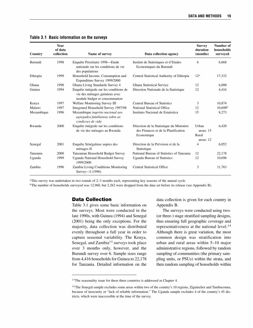
Data CollectionTable 3.1 gives some basic information onthe surveys. Most were conducted in thelate 1990s, with Guinea (1994) and Senegal(2001) being the only exceptions. For themajority, data collection was distributedevenly throughout a full year in order tocapture seasonal variability. The Kenya,Senegal, and Zambia13 surveys took placeover 3 months only, however, and theBurundi survey over 6. Sample sizes rangefrom 4,416 households for Guinea to 22,178for Tanzania. Detailed information on the
data collection is given for each country inAppendix B.
The surveys were conducted using two-(or three-) stage stratified sampling designs,thus ensuring full geographic coverage andrepresentativeness at the national level.14
Although there is great variation, the mostcommon design was stratification intourban and rural areas within 5–10 majoradministrative regions, followed by randomsampling of communities (the primary sam-pling units, or PSUs) within the strata, andthen random sampling of households within
DATA AND METHODS 19
13The seasonality issue for these three countries is addressed in Chapter 4.
14The Senegal sample excludes some areas within two of the country’s 10 regions, Ziguinchor and Tambacouna,because of insecurity or “lack of reliable information.” The Uganda sample excludes 4 of the country’s 45 dis-tricts, which were inaccessible at the time of the survey.
Table 3.1 Basic information on the surveys
Year Survey Number ofof data duration households
Country collection Name of survey Data collection agency (months) surveyed
Burundi 1998 Enquête Prioritaire 1998—Etude Institut de Statistiques et d’Etudes 6 6,668nationale sur les conditions de vie Economiques du Burundides populations
Ethiopia 1999 Household Income, Consumption and Central Statistical Authority of Ethiopia 12a 17,332Expenditure Survey 1999/2000
Ghana 1998 Ghana Living Standards Survey 4 Ghana Statistical Service 12 6,000Guinea 1994 Enquête intégrale sur les conditions de Direction Nationale de la Statistique 12 4,416
vie des ménages guinéens avec module budget et consommation
Kenya 1997 Welfare Monitoring Survey III Central Bureau of Statistics 3 10,874Malawi 1997 Integrated Household Survey 1997/98 National Statistical Office 12 10,698b
Mozambique 1996 Mozambique inqerito nacional aos Instituto Nacional de Estatistica 15 8,273agregados familiareas sobre as condicoes de vida
Rwanda 2000 Enquête intégrale sur les conditions Direction de la Statistique du Ministère Urban 6,420de vie des ménages au Rwanda des Finances et de la Planification areas: 15
Economique Ruralareas: 12
Senegal 2001 Enquête Sénégalaise aupres des Direction de la Prévision et de la 4 6,052ménages II Statistique
Tanzania 2000 Tanzanian Household Budget Survey National Bureau of Statistics of Tanzania 12 22,178Uganda 1999 Uganda National Household Survey Uganda Bureau of Statistics 12 10,696
1999/2000Zambia 1996 Zambia Living Conditions Monitoring Central Statistical Office 3 11,763
Survey—I (1996)
aThis survey was undertaken in two rounds of 2–3 months each, representing key seasons of the annual cycle.bThe number of households surveyed was 12,960, but 2,262 were dropped from the data set before its release (see Appendix B).

communities. When such complex samplingdesigns, rather than simple random sam-pling, are used, it is important to correct forthe design so that any calculated statisticsapply to the population group of interest(Deaton 1997). In this study, samplingweights provided with the surveys andvariables delineating the strata and PSU foreach household were used to correct for thesampling design in the calculation of allfood security measures.15
Table 3.2 gives more details about thedata collection for each country. It showswide variation in the number of food itemsfor which data were collected, the meansof data collection (interview or diary), thesources of food acquisition for which datawere collected, as well as the recall and ref-erence periods for food data collection.
The number of food items ranges froma low of 33 (Burundi) to a high of 274(Malawi). Despite the varying degree ofspecificity in the delineation of food items,they cover all of the food groups making upthe human diet.16 In most surveys the com-monly consumed foods within a food groupare listed individually followed by a resid-ual category to capture all other foods in thegroup. For example, a questionnaire may list“mangoes,” “bananas,” and “oranges” indi-vidually, followed by the item “other fruits.”
Although data were collected on bothfood purchases and consumption of foodfrom home production for all of the coun-tries, in Burundi, Guinea, Kenya, andRwanda, no data were collected on acquisi-tion of food in kind. In Ghana and Uganda,households were asked to report on receipt
of gifts of food. In Ethiopia, Malawi,Mozambique, Senegal, Tanzania, and Zam-bia, they were asked to report on foodsreceived in kind from gifts as well as othersources. For example, the Ethiopia question-naire includes categories for foods receivedfrom governmental organizations, non-governmental organizations, other house-holds, from abroad, collected, in return foremployment, and so forth. Other surveys(for example, Zambia) simply ask for food“received” along with home-produced food.
The recall periods range from 1 day to2 weeks. The only exception among thedata sets considered here is Zambia, whereit is 30 days for maize purchases and 2weeks for all other acquisitions. A recall pe-riod of 1 day is assumed whenever the diarymethod is used. In some cases the recall pe-riod differs for urban and rural households(Guinea, Rwanda, Senegal) or for differentsources of food acquisition (Malawi, Zam-bia). In some surveys, enumerators mademultiple visits to households. For example,for the Guinea and Rwanda surveys, urbanhouseholds were visited 10 times and askedto recall their food acquisition over the last3 days. Rural households, whose monetaryexpenditures are less dependent on a monthlypaycheck, were visited seven times with a2-day recall period. The Ethiopia surveywas undertaken in two rounds, with house-holds visited eight times in each round andgiven a 3- to 4-day recall period.
The reference period of a survey is thetime period over which food data collectiontakes place in total. In the cases where therewas only one visit to each household, the
20 CHAPTER 3
15Questions have been raised about bias in the estimation of the distribution of household energy availabilityacross households when data are derived from a survey with a “complex” sampling design rather than using theequal-probably selection method (Arbia 2003; Naiken 2003; Srivastava, Rai, and Ramasubramanian 2003). How-ever, as pointed out by David (2003) and confirmed by Deaton (Personal communication [e-mail], June 5, 2004),design-unbiased estimates are now standard outputs from modern survey data-processing software. For thisanalysis, all sample means and proportions were calculated using the “svy” commands in STATA Special EditionVersion 8 (StataCorp 2003).
16The foods can be classified into the 12 groups used to construct the diet diversity measure (see Table 2.1). Notethat there is one exception to the above statement among the data sets examined here: the food group “eggs” isnot covered in the Burundi data set.

DATA AND METHODS 21
Table 3.2 Food data collection
Number Meansof food of data Food sources for which Recall period Reference periodb
Country itemsa collection data collected Number of visits (days) (days)
Burundi 33 Interview Purchases, home production 1 15 15
Ethiopia 213 Interview Purchases, home production, in kind 8c 3–4 28
Ghana 109 Diary and Purchases, home production, gifts Literate: 6interview Illiterate: 30 1 30
Guinea 112 Interview Purchases, home production Urban: 10 Urban: 3 Urban: 30Rural: 7 Rural: 2 Rural: 14
Kenya 70 Interview Purchases, home production 1 7 7
Malawi 274 Diary and Purchases, home production, in kind Purchases Purchases Purchases: 14–28interview Literate: 1 Literate: 1 Other: 3
Illiterate: 9 Illiterate: 3Other: 1 Other: 3
Mozambique 217 Interview Purchases, home production, in kind 3 First Visit: 1 7Others: 3
Rwanda 94 Interview Purchases, home production Urban: 10 Urban: 3 Urban: 30Rural: 7 Rural: 2 Rural: 14
Senegal 258 Diary and Purchases, home production, in kind Purchases Purchases Urban: 30interview Literate: 1d Literate: 1 Rural: 21
Illiterate Illiterate: 3Urban: 10 Other: 3Rural: 7
OtherUrban: 10Rural: 7
Tanzania 129 Diary and Purchases, home production, in kind Literate: 2–3 1 30interview Illiterate: 30
Uganda 47 Interview Purchases, home production, gifts 1 7 7
Zambia 40 Interview Purchases, home production, in kind 1 Purchases PurchasesMaize: 30 Maize: 30Rest: 14 Rest: 14Other: 14 Other: 14
aThis is the number of food items used for the final analysis, not the original number listed in the questionnaire. In some cases fewer food itemsare used for the analysis because some had to be combined for conversion to metric quantities.bA survey’s reference period for food data collection is the total time period for which food acquisition is recorded. In the cases where therewas only one visit to each household, the reference period equals the recall period. However, when there were several visits, the reference pe-riod generally equals the number of visits multiplied by the recall period. In the few cases where the diary method was used, the recall periodis 1 day (households are to fill in the diary on a daily basis), and the reference period is the length of time the diary is maintained.cThis survey was undertaken in two rounds. The information here is for each individual round.dThe multiple visits made by the enumerator to households with a literate member were only for recording the diary entries over the last 3 days.

reference period equals the recall period(Burundi, Kenya, Uganda). However, whenthere were several visits, the reference pe-riod generally equals the number of visitsmultiplied by the recall period. In the caseswhere the diary method is used, the refer-ence period is the length of time the diary ismaintained. The most common reference pe-riods for the surveys in this study are 1 week,2 weeks, and 1 month. The only exception isMalawi, for which data on home-producedand in-kind food acquired were collectedusing a 3-day reference period.
Calculation of MetricQuantities of FoodAs discussed in Chapter 2, the raw dataentered from the survey questionnaires—whether expenditures or quantities—must beconverted into metric quantities before theenergy content of food acquired can be de-termined.17 When households are asked toreport expenditures on food acquired only(and not the quantity), expenditure must bedivided by a metric price to derive metricquantities. When they report in terms ofquantities in nonmetric or “local” units ofmeasure, as is usually the case, these quan-tities must be multiplied by the correspond-ing metric weight of the food. Examples oflocal units of measure are heaps, baskets,bundles, calabashes, bowls, bottles, cans(which generally have nonstandard sizes),20-liter tins, and 1-kilogram margarine tins(which have standard sizes). Another com-mon unit of measure is “unity” (also re-ferred to as “piece” or “single”), which iscommonly used when reporting acquisitionof fruits, vegetables, and eggs.
Table 3.3 details the types of food acqui-sition data collected in each survey. Oftenthe approach differs for food purchases, onthe one hand, and home-produced foods andfoods received in kind, on the other. For
purchased food, expenditure data are al-ways collected directly from households or,as in the case of Kenya, can be calculateddirectly by multiplying a food’s reportedlocal quantity by its reported price. In manysurveys quantity in local units is collected aswell. For home-produced foods and foodsreceived in kind, local quantity and unit ofmeasure are always collected, sometimescomplemented by expenditures or price.
To convert to metric quantities, threemethods were used, with the choice ofmethod depending on the type of data col-lected and the availability of complemen-tary data from another source to convert tometric quantities.
Method A: Local Quantity �� Metric WeightThis method was used where householdswere asked to report food quantities, andeither the quantities were reported directlyin metric units (in which case the metricweight is implicit) or they were reported innonstandard units and complementary met-ric conversion factors were available. In thelatter case, metric weights were obtainedfrom one of three sources: (1) weighing ofobservable quantities at the household bythe enumerators, (2) collected in local mar-kets as part of a community price survey, or(3) available from preexisting data bases,such as the United States Department ofAgriculture Nutrient Database for StandardReference, Release 15 (USDA 2003) (forfoods reported in unities) or other surveys.When foods were reported in volumetricmeasures (liters, milliliters), specific gravi-ties from FSANZ (2004) were used to con-vert to metric weights.
Method B: Expenditure/(Metric Price)This method was used to “recover” quanti-ties acquired when households reported their
22 CHAPTER 3
17Tables of the energy composition of foods give calorie conversion factors in units of kilocalories per 100 gramsof food weight.

food expenditures (but not quantities), andcomplementary metric prices were available.Sources of metric prices were (1) derived
from household-reported metric prices orunit values (calculated as expenditure di-vided by metric quantity),18 (2) collected in
DATA AND METHODS 23
18In any given survey, depending on the food, at least some households report directly in metric quantities. If ex-penditures are also available, a metric unit value could be derived as an estimated price. Household-level unit val-ues used to estimate metric prices for other households were used only if at least five households reported a pricefor the food at a given geographic level. For instance, if a metric unit value was available for a food for at leastfive households in a community, then a community price was calculated and used for other households in thecommunity if needed.
Table 3.3 Types of food data collected and methods of conversion to metric quantities
Food purchases Home-produced foods and foods received in kind
Conversion Conversion Country Type of data collected method Type of data collected method
Burundi Expenditure B Quantity, unit of measure A
Ethiopia Quantity, unit of measure, expenditure A (98%) Quantity, unit of measure, expenditure Same as purchasesB (2%)
Ghana Expenditure B Quantity, unit of measure, price A (27%)C (73%)
Guinea Expenditure B Quantity, unit of measure, price A (30%)C (70% )
Kenya Quantity, unit of measure, price A (58%) Quantity, unit of measure, price Same as purchasesB (42%)
Malawi Quantity, unit of measure, expenditure B Quantity, unit of measure, estimated value A (88%)B (12%)
Mozambique Quantity, unit of measure, expenditure A (27%) Quantity, unit of measure, estimated value Same as purchasesB (73%)
Rwanda Expenditure B Quantity, unit of measure, price A (47%)C (53% )
Senegal Quantity, unit of measure, expenditure A (73.8%) Quantity, unit of measure, expenditure Same as purchasesB (24.6%)
Tanzania Quantity, unit of measure, expenditure A (99%) Quantity, unit of measure, expenditure Same as purchasesB (1%)
Uganda Quantity, unit of measure, expenditure A (92%) Quantity, unit of measure, estimated value Same as purchasesC (8%)
Zambia Expenditure B Quantity, unit of measure, price Same as purchases
Notes: Method A: Local quantity × metric conversion factor; Method B: Expenditure/metric price; Method C: Local quantity × (ratio of localto metric price). By “same as purchases” is meant that a distinction between purchases and other sources of acquisition was not madein choice of method for conversions to metric quantities. Thus, the percentage of observations for which each method was used appliesto all observations together, regardless of the source.

local markets as part of a community pricesurvey, or (3) collected as part of a separatesurvey, the most common being a ConsumerPrice Index Survey carried out in all regionsof a country.19
Method C: Local Quantity � Ratioof Local to Metric PriceThis method was used when local quantitieswere available but complementary metricweights were not. The method can either beinterpreted as estimation of a metric weightusing relative prices as a proxy (approxi-mating Method A) or as dividing estimatedexpenditures by a metric price (approxi-mating Method B). For units of measurewith standard sizes, price ratios were takenas the median over all households in thesample with a reported local unit price for afood. For units of measure with nonstandardsizes, price ratios were taken using the localunit price (or calculated unit value in thecase of Uganda) reported at the householdlevel.
Table 3.3 gives the conversion methodsemployed for each survey. Further detailscan be found in Appendix B. The most com-monly employed methods are A and B.Method C is used only for 8 percent of ob-servations in Uganda, roughly 70 percent ofhome-production or in-kind observations inGhana and Guinea, and 53 percent of theseobservations in Rwanda.
The Energy Content of Foods and Energy RequirementsOnce conversion to metric quantities hastaken place, determination of the energy con-tent of foods acquired for consumption inthe home is straightforward. The sources of
calorie conversion factors for each countryare given in Appendix B. Where a countryhas its own food composition table, this isused as the primary source of calorie con-version factors. Where not, the table of anearby country or the Africa food composi-tion table (USDHEW/FAO 1968) was used.In some cases the American food composi-tion table (USDA 2003) was used for foodsknown to vary little in calorie compositionacross countries. The actual energy valueof a food acquired was computed as metricquantity multiplied by the food’s calorievalue, which was then multiplied by thefood’s edible portion. Edible portions aregenerally near 100 percent for grains (in-cluding flours derived from grains) and bev-erages but are lower for fruits, vegetables,roots and tubers, and animal products.
A meta-database containing the calorievalues of all foods encountered in the sur-veys was constructed using available foodcomposition tables from Sub-Saharan Africaas well as the American food compositiontable (USDA 2003). The values were com-pared across sources, and any suspect caseswere dropped. Although the Africa foodcomposition table was created in 1968, itscalorie values are quite consistent with morerecent tables and with the USDA tables,which were compiled using the most up-to-date laboratory techniques.
For foods consumed outside the home,only total expenditures are reported, whichobviously hampers direct conversion to en-ergy values. The only way to take thissource of food acquisition into account is toapply the price per calorie of foods acquiredfor consumption inside the home to the ex-penditures on food consumed outside of thehome. Although this method undoubtedlyreduces the accuracy of estimates of house-
24 CHAPTER 3
19In the context of the Data Food Networking (DAFNE) project, the Irish 1987 Household Budget Survey wasused to show that for a subsample of foods for which metric quantities and expenditures were collected directly,the use of retail prices to convert expenditures to quantities resulted in a 10 percent or less margin of error (Frielet al. 2001).

hold energy availability, it is the approachtaken here by necessity.20
As discussed in Chapter 2, the energyrequirements used are the average energyrequirements of specific age–sex groups forbasal metabolic function and light activity.These are given in Table 3.4, with the re-quirements for moderate and heavy activityalso included for reference. A household’stotal energy requirement is calculated as thesum of the requirements of all householdmembers. An additional 500 calories isadded for each child less than 1 year old
to account for the greater needs of breast-feeding mothers.21
Data CleaningAs discussed in Chapter 2, food acquisitiondata collected in household expenditure sur-veys are subject to a host of errors, fromreporting on the part of households to re-cording on the part of enumerators to enter-ing on the part of data entry operators. Theraw data were subjected to thorough clean-ing so as to avoid any influence of major
DATA AND METHODS 25
20The cost of energy is surely higher away from home because of labor costs, profits, and the fact that higher-cost foods (for example, meat) are more likely to be eaten when away from home. If this difference alone is con-sidered, the estimation method overestimates energy availability from food eaten away. However, the fact that thecaloric value of the foods eaten away is also likely to be higher counteracts the price effect. Thus, the directionof bias from the method is indeterminant without further research.
21Unfortunately the extra energy needs of pregnancy cannot be taken into account because the pregnancy statusof household members was not recorded.
Table 3.4 Recommended daily caloric intakes
Age group Kilocalories per day
Young children<1 8201–2 1,1502–3 1,3503–5 1,550
Older children Boys Girls5–7 1,850 1,7507–10 2,100 1,80010–12 2,200 1,95012–14 2,400 2,10014–16 2,650 2,15016–18 2,850 2,150
Men Light activity Moderate activity Heavy activity18–30 2,600 3,000 3,55030–60 2,500 2,900 3,400>60 2,100 2,450 2,850
Women Light activity Moderate activity Heavy activity18–30 2,000 2,100 2,35030–60 2,050 2,150 2,400>60 1,850 1,950 2,150
Source: FAO/WHO/UNU (1985), as published in Hoddinott (2001).

errors on the estimates of food energy avail-ability. Data cleaning took place in threestages.
First, for each food, weights of foods inlocal units of measure, reported prices, andderived unit values were cleaned manuallyby examination for outliers at both ends ofthe distribution, often separately for eachmajor region of a country. Outlying pricesand weights were set to missing and notused in further calculations. When outlyingunit values were detected, both the expendi-ture and quantity used to calculate themwere set to missing.22
In a second stage, the computed metricquantities of individual foods were cleaned.Any quantity per household adult equiva-lent23 that was more than three standard de-viations from the sample median value wasreplaced with an estimated value using or-dinary least-squares (OLS) regression. Thistechnique was also used to replace valuesset to missing in stage 1 of the data clean-ing. The independent variables in the food-specific regression equations were numberof household adult equivalents, variablesrepresenting the age–sex composition ofthe household, whether it is female headed,age of the household head, whether at leastone adult member has a primary or second-ary education, the number of assets ownedby the household (calculated from survey-specific lists of assets), whether the house-hold is located in an urban area, region ofresidence, and month of survey, where ap-propriate. Note that because this techniquetakes into account household-specific char-acteristics, it preserves variation in the data
better than the more common method ofreplacement with means or medians of otherhouseholds.
The third stage of data cleaning tookplace for household-level energy availability.A household’s total calories per adult equiv-alent was replaced with an estimated valueusing OLS prediction regressions (with thesame regressors as above) when (1) a met-ric quantity that was identified as an outlieror set to missing in the cleaning processcould not be estimated24 or (2) not enoughinformation was available to estimate calo-ries from food consumed outside of thehome25 or (3) a household had no reportedfood acquisition data.
Some households were dropped fromthe analysis altogether. This was the caseif (1) more than 50 percent of the quantitiesof foods it reported were set to missing oridentified as outliers, or (2) its calculateddaily energy per adult equivalent was greaterthan 12,000 kilocalories. Note that no lowerbound was used because it is possible, ifunlikely, for a household to acquire no foodat all over a survey’s reference period.
Table 3.5 summarizes the number ofdropped households and predicted observa-tions for each country. The highest percent-age of households dropped from the analy-sis was 2.5, for Kenya, where 275 of the10,874 sampled households were dropped.The percentages of food acquisition ob-servations with metric quantities estimatedusing prediction regressions are generallyvery low, with the country having the mostbeing, again, Kenya at 6.5 percent. Althoughfor the majority of countries the percentage
26 CHAPTER 3
22The only exception is Senegal, for which quantities were deemed to be the source of the error rather thanexpenditures.
23See next section for the definition of an adult equivalent.
24In some cases, not enough nonmissing observations were available to allow running a regression.
25Households with more than 75 percent of total food expenditures on food acquired outside of the home werenot considered eligible for the “price per calorie of food acquired for consumption in the home” method. Thesehouseholds’ acquisition of in-home food was deemed to be too small, relatively speaking, to use for estimatingacquisition of out-of-home food.

of observations with predicted energy avail-ability is quite low, for Uganda and Ghana,it is near or greater than 10 percent.
Calculation of HouseholdSize and Adult EquivalentsTo calculate household energy availability,the total calories acquired by a household isdivided by either the number of householdmembers or the number of adult equiva-lents. When divided by adult equivalents,the fact that peoples’ energy needs can varysubstantially depending on their sex and ageis taken into account.
A base estimate of the number of house-hold members was first calculated using thedefinition of household membership fol-lowed in the household roster data collec-tion specific to each survey. Following that,an attempt was made to determine the num-ber of people who were actually present inthe household at the time of the survey andthus potentially eating the food acquired.Some surveys directly included informationon which members were present (Burundiand Senegal). Where this information wasnot available, but that on the duration of ab-sence over the last year was, those memberswho were absent for more than 6 monthswere excluded from the household size cal-
culation (Ghana, Guinea, Mozambique,Rwanda, and Uganda). Where no infor-mation was available, the base estimate ofhousehold size was employed. Note that insome of these cases the definition itself in-cluded a condition that members be presentin the household over the last 6 months. An“adult equivalent” is defined using a man30–60 years old as the reference categoryand comparative average energy require-ments for medium activity (see Table 3.4)for the various other age and sex groups.
Household CalorieAvailability: A Look at the Calculated ValuesAs noted in Chapter 2, the data collected inHESs represent household calorie avail-ability rather than intakes. The household-level calculated values for these two vari-ables will look very different from oneanother. Table 3.6 reports descriptive sta-tistics for household daily calorie avail-ability per capita. The means in the tablediffer from those reported in the next chap-ter because (1) they are not corrected forsurvey sampling designs, and (2) they rep-resent household-level calorie availabilityper capita rather than calorie availability percapita per se. Figure 3.2 gives nonparametric
DATA AND METHODS 27
Table 3.5 Data cleaning: Dropped households and predicted values
HouseholdsFood acquisition Households with
Number ofdropped from
Number of observations with predicted energyhouseholds
analysishouseholds retained predicted quantity availability
Country surveyed Number Percentage for analysis (%) (%)
Burundi 6,668 83 1.2 6,585 1.2 1.0Ethiopia 17,332 26 0.2 17,306 2.4 0.12Ghana 6,000 60 1.0 5,940 1.8 9.1Guinea 4,416 44 1.0 4,372 2.0 0.8Kenya 10,874 275 2.5 10,599 6.5 0.4Malawi 10,698 176 1.6 10,522 1.8 15.3Mozambique 8,273 125 1.5 8,148 3.7 0.9Rwanda 6,420 55 0.9 6,365 3.8 0.5Senegal 6,052 45 0.7 6,007 3.7 5.4Tanzania 22,178 528 2.4 21,650 1.3 0.7Uganda 10,696 106 1.0 10,590 4.2 5.8Zambia 11,763 180 1.5 11,583 1.2 0.2
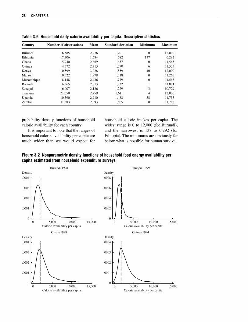
probability density functions of householdcalorie availability for each country.
It is important to note that the ranges ofhousehold calorie availability per capita aremuch wider than we would expect for
household calorie intakes per capita. Thewidest range is 0 to 12,000 (for Burundi),and the narrowest is 137 to 6,292 (forEthiopia). The minimums are obviously farbelow what is possible for human survival.
28 CHAPTER 3
Table 3.6 Household daily calorie availability per capita: Descriptive statistics
Country Number of observations Mean Standard deviation Minimum Maximum
Burundi 6,585 2,276 1,701 0 12,000Ethiopia 17,306 1,684 682 137 6,292Ghana 5,940 2,669 1,657 0 11,565Guinea 4,372 2,713 1,590 6 11,533Kenya 10,599 3,028 1,859 40 12,000Malawi 10,522 1,878 1,518 0 11,265Mozambique 8,148 2,436 1,779 0 11,563Rwanda 6,365 2,013 1,322 1 11,871Senegal 6,007 2,136 1,229 3 10,729Tanzania 21,650 2,759 1,611 4 12,000Uganda 10,590 2,910 1,488 38 11,755Zambia 11,583 2,093 1,505 0 11,785
Figure 3.2 Nonparametric density functions of household food energy availability percapita estimated from household expenditure surveys
.0004
.0004
.0008
.0004
.0003
.0003
.0006
.0003
.0002
.0002
.0004
.0002
.0001
.0001
.0002
.0001
0
0
0
0
0
0
0
0
5,000
5,000
5,000
5,000
10,000
10,000
10,000
10,000
15,000
15,000
15,000
15,000
Calorie availability per capita
Calorie availability per capita
Calorie availability per capita
Calorie availability per capita
Burundi 1998
Ghana 1998
Ethiopia 1999
Guinea 1994
Density
Density
Density
Density

Figure 3.2—Continued
Note: Vertical lines are at the average per capita dietary energy requirement for each country when the aver-age requirement for light activity is assumed.
.0004
.0004
.0004
.0004
.0003
.0003
.0003
.0003
.0002
.0002
.0002
.0002
.0001
.0001
.0001
.0001
0
0
0
0
0
0
0
0
5,000
5,000
5,000
5,000
10,000
10,000
10,000
10,000
15,000
15,000
15,000
15,000
Calorie availability per capita
Calorie availability per capita
Calorie availability per capita
Calorie availability per capita
Senegal 2001
Uganda 1999
Tanzania 2000
Zambia 1996
Density
Density
Density
Density
.0004
.0004
.0003
.0003
.0003
.0003
.0002
.0002
.0002
.0002
.0001
.0001
.0001
.0001
0
0
0
0
0
0
0
0
5,000
5,000
5,000
5,000
10,000
10,000
10,000
10,000
15,000
15,000
15,000
15,000
Calorie availability per capita
Calorie availability per capita
Calorie availability per capita
Calorie availability per capita
Kenya 1997
Mozambique 1996
Malawi 1997
Rwanda 2000
Density
Density
Density
Density

The maximums are far above what a personcould possibly eat in one day. The standarddeviations should theoretically be muchwider than for calorie intakes as well. De-spite these differences, as discussed in Chap-ter 2, we can expect the mean to be the sameregardless of which data source is used be-cause the difference between availability and
intakes is a result of deviations of householdfood acquisitions from consumption that arerandomly distributed across households.Note that the probability distributions ofhousehold calorie availability are skewed tothe right rather than taking on the bell-likeshape of a normal distribution.
30 CHAPTER 3

C H A P T E R 4
Estimates of Food Insecurity
This chapter first presents national estimates of food insecurity and compares them acrossthe 12 countries. It then moves on to look at food insecurity across regions within coun-tries. Finally, it examines differences in the severity of food insecurity for people living
in rural and urban areas, by income group, and for female- and male-headed households.
National Estimates: A Comparison across CountriesTable 4.1 reports on estimates of the diet quantity and quality measures of food securityfor the 12 countries. Starting with diet quantity, energy availability per capita ranges from1,592 kilocalories per person in Burundi (1998) to 2,636 in Uganda (1999). It falls quite nearor below the average energy requirement for light activity (roughly 2,050 kilocalories per per-son) for seven of the countries—Burundi, Ethiopia, Malawi, Mozambique, Rwanda, Senegal,and Zambia—signaling severe food insecurity problems. In these countries there is not enoughfood for all people to meet their requirements even if the food were to be distributed accord-ing to need.
The percentage of people who are food energy deficient ranges from 36.8 percent inUganda to over 75 percent in Burundi and Ethiopia (see Fig. 4.1). The 95 percent confidenceintervals for these estimates are reasonably narrow, with the widest being for Ghana (±3.8 per-centage points from the estimate) (see Table C.2, Appendix C). The estimates are thus quiteprecisely measured. The Spearman correlation coefficient between energy availability percapita and the prevalence of food energy deficiency is –0.96 (P = 0.000), indicating a tightcorrespondence between national-level food availabilities and food energy deficiency in theregion. The percentage of households that are food energy deficient is also given in Table 4.1for reference.26
Clearly, food insecurity is a major problem in all 12 countries. At least one-third, and inmost countries a much higher percentage, of the population is not consuming enough food tomeet requirements for basal metabolic function and light activity.
Uganda, Kenya, Tanzania, Guinea, and Ghana form a cluster of countries with relativelylow rates of food energy deficiency, in the 35–50 percent range. At the time of their surveys,these countries were in a situation of economic and political stability for the most part, withno recent adverse climatic shocks.27 Nevertheless, they were experiencing ongoing problems
26The percentage of households that are food energy deficient is lower than the percentage of people becausehouseholds with low food energy availability tend to be larger.
27An exception is the northern region of Uganda, which was facing insecurity at the time of the survey.
31
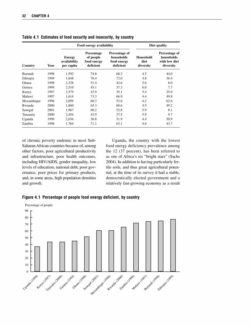
of chronic poverty endemic in most Sub-Saharan African countries because of, amongother factors, poor agricultural productivityand infrastructure, poor health outcomes,including HIV/AIDS, gender inequality, lowlevels of education, national debt, poor gov-ernance, poor prices for primary products,and, in some areas, high population densitiesand growth.
Uganda, the country with the lowestfood energy deficiency prevalence amongthe 12 (37 percent), has been referred toas one of Africa’s six “bright stars” (Sachs2004). In addition to having particularly fer-tile soils, and thus great agricultural poten-tial, at the time of its survey it had a stable,democratically elected government and arelatively fast-growing economy as a result
32 CHAPTER 4
Table 4.1 Estimates of food security and insecurity, by country
Food energy availability Diet quality
Percentage Percentage of Percentage ofEnergy of people households Household households
availability food energy food energy diet with low dietCountry Year per capita deficient deficient diversity diversity
Burundi 1998 1,592 74.8 68.2 4.5 44.0Ethiopia 1999 1,648 76.4 72.0 4.8 36.4Ghana 1998 2,328 51.4 43.6 5.8 8.0Guinea 1994 2,510 45.1 37.3 6.0 7.7Kenya 1997 2,579 43.9 35.1 5.4 25.0Malawi 1997 1,614 73.3 66.9 4.4 49.8Mozambique 1996 2,059 60.3 53.6 4.2 62.6Rwanda 2000 1,860 65.3 60.6 4.5 49.2Senegal 2001 1,967 60.2 52.8 5.9 8.1Tanzania 2000 2,454 43.9 37.5 5.9 9.7Uganda 1999 2,636 36.8 31.9 4.4 50.9Zambia 1996 1,764 71.1 63.1 4.6 43.7
Figure 4.1 Percentage of people food energy deficient, by country

of the economic reform efforts of the Mu-seveni government (FEWS NET 1997;Resnick 2004). At the time of their surveys,Kenya, Tanzania, and Guinea had relativelystrong economies after years of economicreforms. Kenya’s survey, in 1997, followeda year of poor weather conditions in severaldistricts and low prices of maize, its staplecrop. Maize imports were able to make upfor the deficit (UNDHA 1996). Note thatthe survey took place April through Juneof the year, during the countries’ long rains.The harvesting of crops from the short rainstakes place in February and March, whichmay have offset the dip in food availabilitytypically found during the rainy seasons ofcountries with unimodal rainfall patterns.Analysis of the seasonal patterns of energyavailability in neighboring Uganda, whichlies at the same latitude, shows that this timeof year conforms with annual averages.28
Tanzania also experienced poor weatherconditions in the years leading up to itssurvey, including a drought in 1996/97 andEl Nino flooding in 1997/98 (Wobst 2001).Guinea was experiencing the destabilizingeffects of the influx of refugees fleeing fromcivil wars in Liberia and Sierra Leone (U.S.Department of State 2004). Despite 15 yearsof economic reform and democratization inGhana, the collapse of cocoa prices in the1960s and 1970s and the subsequent eco-nomic collapse in the early 1980s has left itwith a weak economy and slow growth inits agricultural sector. Although falling realfood prices over the 1980s and 1990s mayhave improved the food security situation(Nyanteng and Asuming-Brempong 2003),this study nonetheless finds over half of itspopulation to be food energy deficient.
With the exception of Senegal, all of thecountries with aggregate food deficits hadexperienced adverse climatic shocks or se-vere conflict-induced instability in the yearsleading up to their surveys, with long-term
consequences for both food supplies and theability of households to gain access to them.
Ethiopia had been experiencing recurrentdroughts for decades, including that of 1984,which was followed by a devastating faminein which over one million people perished.It had also been experiencing chronic polit-ical instability, including border wars, lead-ing to internal and external refugee crises.The survey year itself was marked by thewar with Eritrea, which exacerbated thecountry’s weak economy. At the time of itssurvey, its poverty rate was among the high-est in the world, at 82 percent (World Bank2003).
At the time of their surveys, Rwandaand Burundi were recovering from ethni-cally motivated civil wars accompanied byviolence and displacements that severelydisrupted food production and completelydevastated people’s livelihoods (UNDHA1996). Economic embargoes against Bu-rundi by neighboring countries exacerbatedthe situation there (World Bank 2004).
Malawi, Zambia, and Mozambique wereall recovering from the effects of severedroughts. The food security situation in thesecountries is also compounded by highprevalences of HIV/AIDS, estimated to be15 percent in Malawi, 22 percent in Zambia,and 13 percent in Mozambique (Zhang et al.2004). Malawi and Zambia, with food en-ergy deficiency prevalences of 73 percentand 71 percent, respectively, share a similarstory of endemic poverty exacerbated byeconomic crisis associated with agriculturalliberalization in the 1980s that hurt smallfarmers and a major drought in 1992–93.The drought led to food shortages, credit de-faulting, and a depletion of household assetsthat had the effect of deepening povertyeven further (Frankenberger et al. 2003).Note that the Zambia survey took place onlyover 3 months during the countries’ dry sea-son, which is usually associated with higher-
ESTIMATES OF FOOD INSECURITY 33
28Mean monthly household food energy availability per capita for the 3 months is 2,901 kilocalories, which isquite close to the mean across all months of 2,877 kilocalories.

than-average food availability. The foodenergy deficiency rate may thus be under-stated, which is confirmed by analysis ofthe seasonal energy availability pattern inneighboring Malawi.29 In addition to expe-riencing the effects of this same drought, atthe time of its survey in 1996, Mozambiquewas recovering from the aftereffects of con-tinuous civil war of 1979–92 that severelydisrupted transport, communications, andmarkets and led to internal and external dis-placements (Arndt, Jensen, and Tarp 2000).
Senegal’s ranking among countries suchas Mozambique and Rwanda is unexpected.This is especially so given that its surveytook place from February through May ofthe year, during the countries’ dry season,when household food availability should beat its highest. However, although it experi-enced no major political or climatic shocksin the years leading up to its survey, itssemiarid climate leaves it with endemicdrought. Water is a basic constraint toagricultural production. Additionally, the1990s witnessed a severe economic reces-sion linked to long-term trends in popula-
tion growth, land degradation, and decliningprices of major exports. This was worsenedby the 1994 CFA devaluation. The growthof its agricultural sector on which mostpeople rely for their livelihoods was slowand variable throughout the 1990s (IFPRI1998), and poverty increased over the decade(Ndiaye 2003).
The diet quality measures show amarkedly different pattern across countriesthan the diet quantity measures (Table 4.1and Fig. 4.2). The household diet diversityscore is lowest for Mozambique, at 4.2 foodgroups out of 7.0, and highest for Guinea, at6.0. Mozambique has the highest prevalenceof households having low diet diversity: 63percent. The West African countries have thelowest prevalences, with the average house-hold’s diet diversity score ranging from 5.8to 6.0 out of the 7 food groups, indicatingquite a varied diet. Less than 10 percent ofthe populations of these countries is classi-fied as having low dietary diversity. With theexception of Tanzania, the East and southernAfrican countries have much higher preva-lences, ranging from 25 to 63 percent.
34 CHAPTER 4
29From the Malawi (1996) survey, annual mean household energy availability is 1,840 kilocalories; that for themonths of August–October is 1,910, 70 kilocalories higher.
Figure 4.2 Prevalence of low diet diversity, by country

Figure 4.3 compares the prevalences offood energy deficiency and low diet diver-sity across the countries. The countries areranked from lowest to highest energy defi-ciency prevalence. For comparability, theseprevalences are for households rather thanfor individuals (see Table 4.1 for the differ-ence). The correlation coefficient betweenthe two measures is low, at 0.43, and notstatistically significant (P = 0.164). Three ofthe countries with high prevalences of foodenergy deficiency—Mozambique, Rwanda,and Malawi—also have very high preva-lences of low diet diversity, near or surpass-ing 50 percent. Three of the countries withrelatively low prevalences of food energydeficiency also have very low prevalencesof low diet diversity (Guinea, Tanzania, andGhana), near or below 10 percent. However,no strong association between the two mea-sures is apparent. A particularly large dis-crepancy in country rankings can be seenfor Uganda, which ranks lowest for foodenergy deficiency but second-to-highest forlow diet diversity. In this country there arelikely substantial numbers of households that
are not experiencing difficulties with accessto sufficient food for meeting their energy re-quirements but that nevertheless have mem-bers who are not able to lead active, healthylives because of diet quality problems. Atthe opposite extreme is Senegal, where aquite high and middling-ranked food energydeficiency rate is coupled with one of thebottommost rates of low diet diversity.
The absence of a strong association be-tween the diet quantity and quality indica-tors suggests that these two aspects of foodinsecurity have quite different distributionsacross households as well as determinants.The differences may be associated with cul-tural traditions governing eating habits, cli-matic conditions governing food productionvariety, or availability of a variety of foodsin local markets. They may also be associ-ated with differences in socioeconomic de-terminants such as income and education.
Subnational Estimates:Looking within CountriesAppendix D contains food security pro-files for the 12 countries that give the diet
ESTIMATES OF FOOD INSECURITY 35
Figure 4.3 Prevalences of food energy deficiency and low diet diversity, by country
Note: The food energy deficiency prevalences differ from those given in Figure 4.1 in that they represent thepercentage of households that are food energy deficient rather than of people (see Table 4.1).

quantity and quality estimates for each coun-try’s main regions, by urban and rural resi-dence, by total expenditure quintile, and bymale- and female-headed household. In ad-dition to the measures of focus in this study,two others are reported: (1) the percentageof energy from staples, a measure of dietquality, and (2) the percentage of expendi-tures on food, which is a measure of eco-nomic vulnerability to food insecurity.30
Regions within CountriesEthiopia’s high prevalence of food energydeficiency applies to all of its regions. Thelowest prevalence is 66 percent in the Ben-ishangul Gumuz region, and the highest isfound in the Afar region, where 90 percentof all people are energy deficient. Similarly,Kenya’s relatively low prevalence is fairlyconstant across its regions. The fertile cen-tral region has among the lowest rates offood energy deficiency, at roughly one-thirdof the population. Prevalences in the denselypopulated Western and arid Rift Valley prov-inces are slightly above 50 percent but stillmoderate, relatively speaking.
However, for many of the countriesnational food insecurity prevalences maskwithin-country variability that is importantto take into account in food security policydecisionmaking. Despite Uganda’s rela-tively low national rate of food energy defi-ciency (37 percent), nearly 60 percent ofpeople in its northern region, which ex-perienced conflict-induced instability anddrought in the years preceding the survey,do not have access to sufficient food. Mo-zambique has particularly large extremes,with the Gaza region in the high-agricultural-productivity south having a food energydeficiency rate of 36 percent and CaboDelgado in the low-productivity north (Gar-rett 1998) having a rate of near 75 percent.
Guinea’s “Guinee Forestiere” region standsout from its other regions as having a rela-tively low prevalence of food energy defi-ciency (27 percent).
The diet quality measures show the samedual pattern, with some countries showingcommonality across their regions and othersgreat variability. The regions within Ghanaand Guinea in West Africa show fairly com-mon small prevalences of low diet diversity.Among the countries with very high preva-lences nationally, variations among regionsis quite high. Rwanda has one region (out-side of the capital) that is doing far betterthan the others, Cyangugu, which has a lowdiet diversity rate of 21 percent comparedwith the national average of 50 percent.
In the example of Tanzania, Figures 4.4and 4.5 present food insecurity maps to il-lustrate the wide variability that can be foundwithin countries as well as the differing dis-tributions of food energy deficiency and lowdiet diversity within them. The extremes offood energy deficiency prevalences run fromas low as 22 percent in Tabora, the regionwith the lowest incidence of poverty (NBST2002) to as high as 61 percent in the regionof Kilimanjaro. The latter region is amongseveral cereal-dependent north-central re-gions for which there was a decline in cerealproduction in the season immediately be-fore the survey because of delayed rains(FAO 1999; Tanzania 2000).
With respect to diet quality, Tabora isagain identified as a region with one of thelowest incidences of food insecurity. Thehighest rates of low diet diversity are foundin the three most southern regions of thecountry (Lindi, Ruvuma, and Mtwara), inthe lake region of Mara, and in Singida.Lindi has the highest rate, at 20.5 percent,associated with one of the highest rates ofpoverty, and the three southern regions are
36 CHAPTER 4
30Households that spend high proportions of their incomes on food (say 70 percent or more) are vulnerablebecause if food prices are increased or their income is reduced, for example, through a job loss, natural disaster,or disease onset (for example, HIV/AIDS), they will have limited reserve for meeting their food needs (Maxwellet al. 1999).
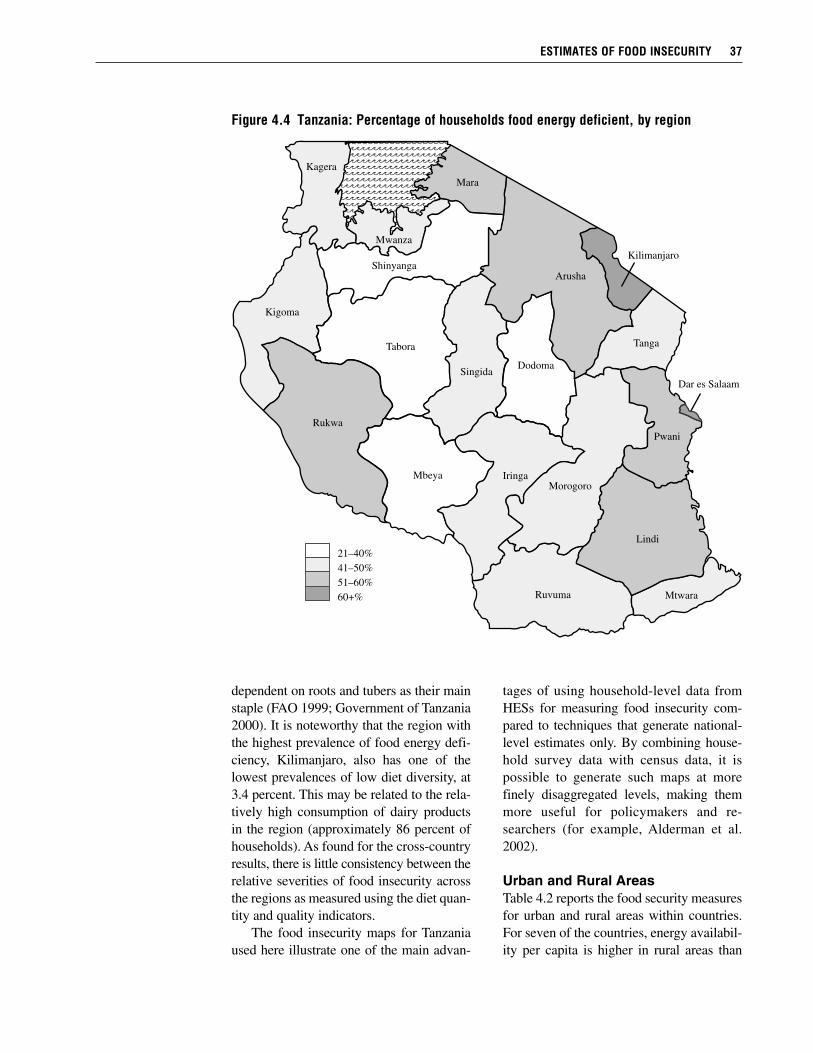
dependent on roots and tubers as their mainstaple (FAO 1999; Government of Tanzania2000). It is noteworthy that the region withthe highest prevalence of food energy defi-ciency, Kilimanjaro, also has one of thelowest prevalences of low diet diversity, at3.4 percent. This may be related to the rela-tively high consumption of dairy productsin the region (approximately 86 percent ofhouseholds). As found for the cross-countryresults, there is little consistency between therelative severities of food insecurity acrossthe regions as measured using the diet quan-tity and quality indicators.
The food insecurity maps for Tanzaniaused here illustrate one of the main advan-
tages of using household-level data fromHESs for measuring food insecurity com-pared to techniques that generate national-level estimates only. By combining house-hold survey data with census data, it ispossible to generate such maps at morefinely disaggregated levels, making themmore useful for policymakers and re-searchers (for example, Alderman et al.2002).
Urban and Rural AreasTable 4.2 reports the food security measuresfor urban and rural areas within countries.For seven of the countries, energy availabil-ity per capita is higher in rural areas than
ESTIMATES OF FOOD INSECURITY 37
Figure 4.4 Tanzania: Percentage of households food energy deficient, by region
21–40%41–50%51–60%60+%
aaaaaaaaaaaaaaaaaaaaaa
aaaaaaaaaaaaaaaaaaaaaa
aaaaaaaaaaaaaaaaaaaaaa
aaaaaaaaaaaaaaaaaaaaaa
aaaaaaaaaaaaaaaaaaaaaa
aaaaaaaaaaaaaaaaaaaaaa
aaaaaaaaaaaaaaaaaaaaaa
aaaaaaaaaaaaaaaaaaaaaa
aaaaaaaaaaaaaaaaaaaaaa
aaaaaaaaaaaaaaaaaaaaaa
aaaaaaaaaaaaaaaaaaaaaa
aaaaaaaaaaaaaaaaaaaaaa
aaaaaaaaaaaaaaaaaaaaaa
aaaaaaaaaaaaaaaaaaaaaa
aaaaaaaaaaaaaaaaaaaaaa
aaaaaaaaaaaaaaaaaaaaaa
Ruvuma
Dar es Salaam
Kilimanjaro
Arusha
Tanga
DodomaSingida
IringaMorogoro
Lindi
Pwani
Mtwara
Kigoma
Rukwa
Tabora
Mbeya
Kagera
Mwanza
Shinyanga
Mara

urban despite the fact that urban areas areknown to have lower poverty rates. In fact,urban dwellers may have lower energy con-sumption than rural dwellers because theyare more dependent on purchased foods thatoften have higher prices than in rural areas.Further, rural dwellers are more physicallyactive and thus consume more energy andmore energy-dense foods (starchy staples)in order to meet their higher actual (ratherthan normative) energy requirement (Hig-gins and Alderman 1997). When it comesto urban–rural differences in the prevalenceof food energy deficiency, it must be kept inmind that this study uses an energy require-
ment for basal metabolic function and lightactivity, a minimum normative requirementbelow which a person is defined to be foodenergy deficient regardless of his or heractual activity level. Thus, urban–rural differ-ences in the prevalence of food energy defi-ciency could go either way, as is found here.For four of the eight countries with substan-tial urban–rural differences in food energydeficiency—Burundi, Kenya, Mozambique,and Rwanda—prevalences are higher in ruralareas. The difference is particularly high forBurundi, in which the percentage of ruraldwellers who are deficient is 76 percent,while the percent of urbanites who are defi-
38 CHAPTER 4
Figure 4.5 Tanzania: Percentage of households with low diversity, by region
Less than 6%7–12%13–15%16+%
aaaaaaaaaaaaaaaaaaaaaa
aaaaaaaaaaaaaaaaaaaaaa
aaaaaaaaaaaaaaaaaaaaaa
aaaaaaaaaaaaaaaaaaaaaa
aaaaaaaaaaaaaaaaaaaaaa
aaaaaaaaaaaaaaaaaaaaaa
aaaaaaaaaaaaaaaaaaaaaa
aaaaaaaaaaaaaaaaaaaaaa
aaaaaaaaaaaaaaaaaaaaaa
aaaaaaaaaaaaaaaaaaaaaa
aaaaaaaaaaaaaaaaaaaaaa
aaaaaaaaaaaaaaaaaaaaaa
aaaaaaaaaaaaaaaaaaaaaa
aaaaaaaaaaaaaaaaaaaaaa
aaaaaaaaaaaaaaaaaaaaaa
aaaaaaaaaaaaaaaaaaaaaa
Ruvuma
Dar es Salaam
Kilimanjaro
Arusha
Tanga
DodomaSingida
IringaMorogoro
Lindi
Pwani
Mtwara
Kigoma
Rukwa
Tabora
Mbeya
Kagera
Mwanza
Shinyanga
Mara

cient is 41 percent. For the other four coun-tries (Ethiopia, Guinea, Senegal, and Tanza-nia), the opposite is true.
Note that because urban–rural differ-ences in actual energy requirements asso-ciated with energy expenditures cannot betaken into account, we cannot infer fromthe above results that urbanites are morefood insecure than rural dwellers, only thatthere are more urban households for whichthe light activity requirement is not met. Itshould also be noted that because of therelatively low level of urbanization in Sub-Saharan Africa, the absolute numbers ofenergy-deficient people in rural areas is stillhigher than those in urban areas (Ruel andGarrett 2004). Urban households have aclear advantage when it comes to diet qual-ity. Their mean diet diversity score is 5.9,
whereas that for rural households is 4.8, andin all countries it is higher in urban areas.Similarly, in all countries except Ghana,where the urban rate is just slightly higherthan the rural rate, the percentage of house-holds with low diet diversity is higher inrural areas. In addition to higher urban in-comes, this can be explained by the betteraccess to a wider variety of foods in closeproximity in urban areas. Rural householdsare more likely to rely on their own produc-tion or to live farther away from marketswhere a variety of foods can be purchased.
Income GroupsWe turn next to look at how the food secu-rity indicators differ across income groups,as defined by total expenditure quintiles.31 Inconstructing the quintiles we use predicted
ESTIMATES OF FOOD INSECURITY 39
31Households’ total and food expenditures were provided by the various government statistical agencies. Sub-sequently, total expenditures were recalculated after the original food expenditures had been replaced with thatcalculated as part of this study.
Table 4.2 Urban–rural differences in estimates of food security and insecurity
Food energy availability Diet quality
Energy Percentage of Percentage ofavailability people food Household households withper capita energy deficient diet diversity low diet diversity
Country Year Rural Urban Rural Urban Rural Urban Rural Urban
Burundi 1998 1,539 2,674 76.2 41.3 4.4 5.9 46.0 6.5Ethiopia 1999 1,680 1,444 74.4 89.2 4.7 5.5 40.0 15.2Ghana 1998 2,358 2,269 50.5 53.1 5.7 6.0 7.6 8.6Guinea 1994 2,645 2,234 40.6 54.3 5.8 6.6 9.7 3.5Kenya 1997 2,473 3,168 46.3 30.2 5.2 5.9 28.2 12.0Malawi 1997 1,621 1,533 73.0 76.3 4.2 5.7 53.6 16.8Mozambique 1996 1,935 2,524 62.9 50.7 4.0 5.1 70.1 29.3Rwanda 2000 1,824 2,159 66.5 55.4 4.3 6.3 54.1 4.9Senegal 2001 2,065 1,827 54.3 68.5 5.6 6.3 11.0 4.3Tanzania 2000 2,487 2,314 41.8 52.7 5.8 6.2 11.0 5.1Uganda 1999 2,658 2,493 36.3 40.7 4.2 5.3 56.5 21.1Zambia 1996 1,750 1,788 71.2 70.9 4.1 5.6 60.9 11.8
Mean 2,091 2,203 58.1 57.1 4.8 5.9 37.4 11.6
Note: All values are corrected for survey sampling designs.

total expenditures per capita32 rather thanactual expenditures, applying the standardinstrumental variables regression procedureused in the presence of measurement error(Green 1997). This approach is followedto overcome two measurement problemsdiscussed in Chapter 2. The first is randommeasurement error associated with transitoryexpenditure fluctuations such that currentexpenditures can deviate greatly from long-run expenditures (Behrman and Knowles1997; Filmer and Pritchett 1998). The fluc-tuations are most apparent in food expendi-tures, which make up a large percentage ofhouseholds’ total expenditures, manifestingitself in the availability–consumption gapassociated with the drawing-down and ac-cumulation of stocks. Unless these arecorrected for, relatively rich householdsthat happen to acquire very little food andother goods over the reference period ofthe survey could erroneously be classifiedas falling into the bottom quintiles and viceversa. The second problem is that of sys-tematic measurement error caused by thefact that data are not collected on food givento pets and guests or wasted, which is greaterfor richer households (Bouis and Haddad1992). In either case, estimates of food se-curity indicators across the quintiles can behighly biased, causing the differences amongthe quintiles to be exaggerated. Note that inregard to calorie availability per capita, thecorrection made here is similar to that usedto eliminate upward bias in calorie-incomeelasticities.
For the interested reader the estimates ofthe food security indicators across the quin-tiles when actual rather than predicted totalexpenditures are used to classify households
into quintiles can be found in Appendix F,Table F.1. As can be seen there, for manycountries estimates of daily energy consump-tion per capita are unreasonably low in thebottom quintile and/or unreasonably high inthe top quintile. In the example of Burundi,the estimate for the bottom quintile is 688kilocalories, far below the amount anyhuman being could survive on. This quintileundoubtedly contains the survey householdsthat were acquiring very little food over thesurvey reference period but neverthelesswere drawing down on previously acquiredfood stocks to meet current consumptionneeds. The estimate for the top quintile is4,055 kilocalories, above the amount thatmost human beings could comfortably eatin 1 day on a regular basis. This quintilecontains households that were building uptheir food stocks during the survey refer-ence period. Table 4.3 shows the resultswhen predicted total expenditures are usedto classify households into quintiles. Thenew bottom and top quintile estimates ofcalorie consumption for Burundi are morereasonable, at 1,193 and 3,683 kilocalories,respectively.
In regard to the analysis at hand, thepercentage of people food energy deficientgenerally falls dramatically across house-holds from the bottom 20 percent of theincome distribution to the top 20 percent(Table 4.3, column 2). The average food en-ergy deficiency prevalence of the bottomquintile is 67 percent; that of the top is 40percent. Burundi displays a particularly largedegree of inequality across the quintiles,with 86 percent of people in the bottom quin-tile food energy deficient and only 14 per-cent in the top quintile. For some countries,
40 CHAPTER 4
32They are predicted using as instruments asset ownership as well as other longer-run characteristics of house-holds such as education, household demographics, and region of residence. The number of assets for which datawere collected varies from 9 (Uganda) to 27 (Tanzania). For the asset ownership measure a simple additive, percapita index is created, where ownership dummy variables taking values of 0 or 1 are summed and divided bythe number of household members. Note that only “consumption” assets (such as radios, bicycles, and householdappliances) are used rather than “productive” assets (e.g., hoes) because including the latter would make ruralhouseholds that rely on agricultural production as their main source of income appear to be relatively better offthan urban households.
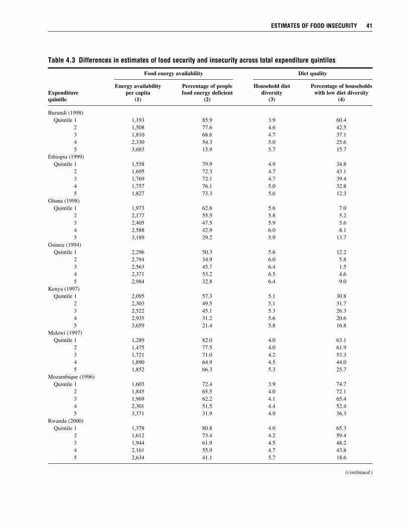
ESTIMATES OF FOOD INSECURITY 41
Table 4.3 Differences in estimates of food security and insecurity across total expenditure quintiles
Food energy availability Diet quality
Energy availability Percentage of people Household diet Percentage of householdsExpenditure per capita food energy deficient diversity with low diet diversityquintile (1) (2) (3) (4)
Burundi (1998)Quintile 1 1,193 85.9 3.9 60.4
2 1,508 77.6 4.6 42.53 1,810 68.6 4.7 37.14 2,330 54.3 5.0 25.65 3,683 13.9 5.7 15.7
Ethiopia (1999)Quintile 1 1,558 79.9 4.9 34.8
2 1,695 72.3 4.7 43.13 1,769 72.1 4.7 39.44 1,757 76.1 5.0 32.85 1,827 73.3 5.6 12.3
Ghana (1998)Quintile 1 1,973 62.6 5.6 7.0
2 2,177 55.5 5.8 5.23 2,405 47.5 5.9 5.64 2,588 42.9 6.0 8.15 3,189 29.2 5.9 13.7
Guinea (1994)Quintile 1 2,296 50.3 5.6 12.2
2 2,794 34.9 6.0 5.83 2,563 45.7 6.4 1.54 2,371 53.2 6.5 4.65 2,984 32.8 6.4 9.0
Kenya (1997)Quintile 1 2,095 57.3 5.1 30.8
2 2,303 49.5 5.1 31.73 2,522 45.1 5.3 26.34 2,935 31.2 5.6 20.65 3,659 21.4 5.8 16.8
Malawi (1997)Quintile 1 1,289 82.0 4.0 63.1
2 1,475 77.5 4.0 61.93 1,721 71.0 4.2 53.34 1,890 64.9 4.5 44.05 1,852 66.3 5.3 25.7
Mozambique (1996)Quintile 1 1,603 72.4 3.9 74.7
2 1,845 65.5 4.0 72.13 1,969 62.2 4.1 65.44 2,301 51.5 4.4 52.45 3,371 31.9 4.9 36.3
Rwanda (2000)Quintile 1 1,378 80.8 4.0 65.3
2 1,612 73.4 4.2 59.43 1,944 61.9 4.5 48.24 2,161 55.9 4.7 43.85 2,634 41.1 5.7 18.6
(continued )
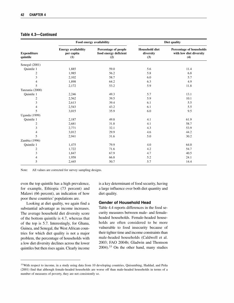
even the top quintile has a high prevalence,for example, Ethiopia (73 percent) andMalawi (66 percent), an indication of howpoor these countries’ populations are.
Looking at diet quality, we again find asubstantial advantage as income increases.The average household diet diversity scoreof the bottom quintile is 4.7, whereas thatof the top is 5.7. Interestingly, for Ghana,Guinea, and Senegal, the West African coun-tries for which diet quality is not a majorproblem, the percentage of households witha low diet diversity declines across the lowerquintiles but then rises again. Clearly income
is a key determinant of food security, havinga large influence over both diet quantity anddiet quality.
Gender of Household HeadTable 4.4 reports differences in the food se-curity measures between male- and female-headed households. Female-headed house-holds are often considered to be morevulnerable to food insecurity because oftheir tighter time and income constraints thanmale-headed households (Caldwell et al.2003; FAO 2004b; Gladwin and Thomson2004).33 On the other hand, many studies
42 CHAPTER 4
33With respect to income, in a study using data from 10 developing countries, Quisumbing, Haddad, and Peña(2001) find that although female-headed households are worse off than male-headed households in terms of anumber of measures of poverty, they are not consistently so.
Table 4.3—Continued
Food energy availability Diet quality
Energy availability Percentage of people Household diet Percentage of householdsExpenditure per capita food energy deficient diversity with low diet diversityquintile (1) (2) (3) (4)
Senegal (2001)Quintile 1 1,885 59.0 5.6 11.4
2 1,985 56.2 5.8 6.83 2,102 58.7 6.0 5.74 1,898 64.2 6.3 4.95 2,172 53.2 5.9 11.8
Tanzania (2000)Quintile 1 2,246 49.3 5.7 13.1
2 2,562 39.5 5.9 10.13 2,613 39.4 6.1 5.54 2,543 43.2 6.1 5.55 3,015 35.9 6.0 9.5
Uganda (1999)Quintile 1 2,187 49.8 4.1 61.9
2 2,681 31.8 4.1 58.73 2,771 32.1 4.3 53.94 3,012 29.9 4.6 44.25 2,941 31.6 5.0 30.2
Zambia (1996)Quintile 1 1,475 79.9 4.0 64.0
2 1,722 71.6 4.2 54.73 1,847 67.9 4.7 40.54 1,958 66.8 5.2 24.15 2,445 50.7 5.7 14.4
Note: All values are corrected for survey sampling designs.

find that when women have the power tomake decisions over the allocation of re-sources, which they do more in female-headed households, they tend to allocatetheir scarce resources toward goods thatbenefit the entire household, such as food,rather than only themselves (Haddad, Hod-dinott, and Alderman 1997).
Table 4.4 shows that, on average, fe-male-headed households have about thesame rates of food energy deficiency asmale-headed households. For three of thecountries where there is a substantial differ-
ence (Ghana, Guinea, and Kenya), the rateis substantially higher for male-headedhouseholds. In Burundi, Rwanda, Senegal,and Uganda, the opposite is true. In terms ofdiet quality, outside of West Africa, whereprevalences of low diet diversity are verylow, female-headed households are doingworse than male-headed households in allbut one country, Mozambique. These find-ings indicate that in East and southern Africafemale-headed households are likely to bea vulnerable group when it comes to dietquality.
ESTIMATES OF FOOD INSECURITY 43
Table 4.4 Differences in estimates of food security and insecurity for female- and male-headed households
Food energy availability Diet quality
Energy Percentage of Percentage ofavailability people food Household diet households withper capita energy deficient diversity low diet diversity
Country Year Male Female Male Female Male Female Male Female
Burundi 1998 1,654 1,395 73.4 78.3 4.7 4.0 39.2 57.6Ethiopia 1999 1,653 1,628 76.4 76.2 4.9 4.7 34.6 41.5Ghana 1998 2,327 2,333 52.4 48.7 5.8 5.9 8.5 6.9Guinea 1994 2,496 2,625 45.6 40.7 6.0 5.9 6.9 12.0Kenya 1997 2,581 2,572 45.2 39.7 5.4 5.2 23.4 29.0Malawi 1997 1,631 1,546 73.1 74.2 4.5 4.2 47.3 57.6Mozambique 1996 2,045 2,124 60.8 58.2 4.2 4.2 62.6 62.4Rwanda 2000 1,903 1,746 64.1 68.6 4.7 4.3 45.2 57.9Senegal 2001 1,986 1,868 59.5 63.7 5.9 6.1 8.2 7.4Tanzania 2000 2,460 2,427 44.2 42.8 5.9 5.9 9.6 10.1Uganda 1999 2,687 2,460 34.7 44.4 4.5 4.2 48.6 57.2Zambia 1996 1,762 1,774 71.5 69.2 4.7 4.3 40.8 53.1
Mean 2,103 2,045 58.7 59.0 5.1 4.9 31.2 37.7
Note: All values are corrected for survey sampling designs.

C H A P T E R 5
Comparison with FAO Estimates and Related Measures
The first section of this chapter starts out by comparing household expenditure survey(HES) and Food and Agricultural Organization of the United Nations (FAO) estimatesof national prevalences of food energy deficiency. The latter is being used to monitor
progress on Millennium Development Goal (MDG) number one, to eradicate extreme povertyand hunger. The HES and FAO methods are used to estimate the same measure. We wouldthus expect them to have a strong positive association with one another. This is not the case,however, and the aim of the second section is to give some insights into why. The chapter nextcompares HES and FAO estimates for the study countries to two other indicators being usedto monitor MDG goal number 1, poverty and child malnutrition prevalences, and to countryrankings based on an expert opinion survey.
Comparison of HES and FAO Estimates of Food Energy DeficiencyTable 5.1 compares HES and FAO estimates of food energy deficiency. Figure 5.1 shows themgraphically, with countries ranked from lowest to highest by the HES estimate. For some ofthe countries, they are quite close; for example, Kenya, Tanzania, and Mozambique. For others,however, they are far apart, with the greatest difference being for Malawi, where the FAO es-timate is 41 percentage points below the HES estimate. Other countries with particularly largedifferences are Ghana, Senegal, and Ethiopia. In all cases where there are substantial differ-ences between the estimates, FAO estimates of food energy deficiency are lower. The meanHES–FAO estimate difference is quite substantial, at 20 percentage points.
Overall, there appears to be a weak correspondence between the HES and FAO estimates.Their Pearson correlation coefficient is 0.46 and is not statistically significant (P = 0.136).Clearly, the two methods of measuring this aspect of food insecurity yield quite differentpictures of its magnitude for the study countries. Further, the country rankings implied by thetwo sets of estimates give conflicting information about relative severities and thus appropri-ate targeting strategies for international agencies and initiatives with the objective of reducingfood insecurity in Sub-Saharan Africa.
Why Do the HES and FAO Estimates Differ? Some First InsightsAn in-depth investigation of this question is beyond the scope of this report. However, wecan gain some initial insights by looking more closely at the method used to generate the FAO
44

COMPARISON WITH FAO ESTIMATES AND RELATED MEASURES 45
Table 5.1 Comparison of HES and FAO estimates of national prevalences of food energy deficiency
HES estimate FAO estimate DifferenceCountry Year (%) (%) (percentage points)
Ethiopia 1999 76.4 44 32.4Burundi 1998 74.8 66 8.8Malawi 1997 73.3 32 41.3Zambia 1996 71.1 45 26.1Rwanda 2000 65.3 41 24.3Mozambique 1996 60.3 63 2.7Senegal 2001 60.2 24 36.2Ghana 1998 51.4 15 36.4Guineaa 1994 45.1 31 14.1Kenya 1997 43.9 43 0.9Tanzania 2000 43.9 43 0.9Uganda 1999 36.8 21 15.8
Mean 58.5 39 19.5
Note: Household expenditure survey (HES) estimates are from the AFINS project food security database. Foodand Agriculture Organization of the United Nations (FAO) estimates are from FAO (1999–2002).
aThe FAO estimate is for 1995–97, before country-level estimates began to be reported. There were no majorchanges in the country’s per capita dietary energy supply—on which the FAO measure is based—over 1994–97.
Figure 5.1 Comparison of HES and FAO estimates of national prevalences of foodenergy deficiency
Source: See notes to Table 5.1.
estimates. This method is a “parametric”method, meaning that it relies on the use ofparameters describing a distribution of avariable of interest in a population. The dis-tribution is assumed to follow a particularshape. The method used in this report, bycontrast, is referred to as “nonparametric,”relying directly on the data for estimationof statistics describing a variable (Statsoft2005). In this section, after describing theFAO method, we investigate why estimatesof food energy deficiency based on the twomethods differ by comparing the parametersemployed in the FAO method with those de-rived from the HES data or assumed for theHES method. We then recalculate the FAOestimates using the HES parameters to get asense of the influence of the parameter dif-ferences on the divergences in food energydeficiency estimates.
FAO Method: The Log-NormalProbability Distribution FrameworkThe method relies on the following key as-sumptions (Naiken 2003):• Dietary energy consumption is distrib-
uted across each country’s populationaccording to a two-parameter log-normal probability distribution, wherethe key parameters are the mean andthe coefficient of variation (CV) (stan-dard deviation divided by the mean).
• The mean of the distribution is thedaily dietary energy available per per-son in the country, referred to as the“dietary energy supply” (DES).
• The CV of the distribution can berepresented by the variation across the population in food consumptionattributable to two sources: house-hold incomes and household energyrequirements.
• The dietary energy requirement of thepopulation corresponds to the age–sexgroup weighted average of the mini-
mum energy requirement for light ac-tivity (corresponding to the lower limitof the range of acceptable body weightfor a given height).34
• The area under the log-normal distribu-tion to the left of the energy requirementgives the proportion of the populationthat is food energy deficient.
The method is illustrated in Figure 5.2.Mathematically, the proportion of peoplefood energy deficient is calculated as follows.Let µi
* be country i’s DES and CVi* be the
country’s coefficient of variation of dietaryenergy consumption. Then the standard de-viation (σi) and mean (µi) of country i’slog-normal distributions are calculated as:
σi = √ln(CVi*2 + 1)
σi2
µi = ln(µi*) – —–
2
These values are used to compute a z-score:
ln(zi) – µiz – scorei = ———— i = 1, . . . , N,σi
which can be looked up in a table of standardnormal probabilities to find the estimatedproportion of energy-deficient people.
Comparison of Dietary EnergyRequirements EmployedThe dietary energy requirement used for theFAO method is lower than that used in thisreport even though the same “light” activitylevel is assumed. Recall that the FAO/WHO/UNU (1985) requirements are basedon a normatively specified body weightconsistent with good health for each activitylevel. However, for a given height, there isa range of body weights that are consistentwith good health. Therefore, there is a rangeof requirements for adults and adolescents
46 CHAPTER 5
34For under-10-year-olds, the median, rather than minimum, of the range is employed. An extra 5 percent al-lowance for optimum activity levels for children specified by FAO/WHO/UNU (1985) is removed (Naiken 2003).

at each acceptable weight-for-height andphysical activity level. FAO uses the lowestacceptable requirement, referred to as theminimum energy requirement for light ac-tivity (corresponding to the fifth percentileof the body mass index).35 The nationaldietary energy requirement is a weightedaverage of the age- and sex-specific mini-mum requirements using population propor-tions as weights (Naiken 2003). The aim isto identify individuals who are at a “high”or “unacceptable” risk of food energy defi-ciency. In this approach, any person fallingbelow the minimum requirement of her orhis age–sex group is undoubtedly food en-ergy deficient. However, those who are notmeeting their requirement but are still abovethat of the lowest-weight person in their age–sex group are erroneously classified as notbeing food energy deficient. Thus, when aminimum requirement is used many foodinsecure people are missed.
The requirements used in this study arethe average energy requirements for lightactivity of each age-sex group, as recom-
mended by the FAO/WHO/UNU (1985)consultation. In contrast to those used byFAO, the aim is to identify people fallingbelow where they should be. As discussedin Chapter 2, this also leads to some classi-fication error because the people whose in-dividual requirement is below the averagemay be wrongly classified as food energydeficient and those whose requirement isabove may be wrongly classified as not en-ergy deficient. If the numbers of people inthese groups are roughly the same, the errorswill cancel each other out and not influencethe calculation of the percentage of a popu-lation that is food energy deficient (Mason2003). However, further research is neededto determine the bias entailed, if any.
Table 5.2 compares HES and FAO es-timates of national dietary energy require-ments. HES estimates are calculated as theaverage person’s energy requirement in eachsurvey’s sample, corrected for the samplingdesign. The mean of the FAO requirementsacross the countries is 1,808 kilocalories,ranging from 1,720 for Ethiopia to 1,890
COMPARISON WITH FAO ESTIMATES AND RELATED MEASURES 47
35Note that for children below 10 years, the median of the range of weight-for-height is used rather than the lowerlimit because a range was not specified for this group. The requirements are currently under review based on the2001 Expert Consultation on Human Energy (FAO 2004a).
Figure 5.2 FAO log-normal distribution framework

for Mozambique. The mean of the HES re-quirements is 2,046—237 kilocalories higherthan the FAO estimate.
Comparison of Mean DietaryEnergy ConsumptionThe mean of the log-normal distribution forany year used in the FAO approach is esti-mated as countries’ DESs in kilocaloriesper capita during the year. It is derived fromfood balance sheets compiled annually byFAO using data on the production and tradeof food. The quantities of foods availablefor human consumption are calculated afterthe use for seed and animal feed, wastagerates, and stock changes are taken into ac-count. The estimated energy available perperson is then obtained by converting thevalues to their dietary energy content anddividing by the population size.
Recall that, as discussed in Chapter 2, thedata collected in HESs generate estimates ofmean household dietary energy availabilitythat are unbiased estimates of mean dietaryenergy consumption. Thus, the FAO andHES estimates should theoretically be quiteclose.
Table 5.3 compares FAO and HES esti-mates of national per capita dietary energyconsumption, with the countries ordered bythe magnitude of the difference. The HESestimates are calculated as the survey design–corrected mean of the energy available toeach person in the sample, which itself isestimated as the per capita energy avail-ability of each person’s household. Althoughthe average difference (last column) is quitesmall, at 40 kilocalories, many of the coun-try differences are substantial, the largestbeing for Kenya (598 kilocalories), Tanza-nia (496 kilocalories), and Malawi (–433kilocalories). The only country for whichlittle disparity was found is Burundi. Noconsistent pattern in the direction of thedifference can be detected: for roughly halfof the countries for which there is a sub-stantial difference it is negative, and for theother half it is positive.
One explanation that has been given forthe difference in FAO and HES estimatesof the energy available for human consump-tion is that food balance sheets measure itat a completely different level of the foodsystem, including nonhousehold use (FAO
48 CHAPTER 5
Table 5.2 Comparison of HES and FAO estimates of national percapita dietary energy requirement (kilocalories ⋅⋅ person–1 ⋅⋅ day–1)
Country Year HES FAO Difference
Mozambique 1996 2,048 1,890 158Guinea 1994 2,026 1,830 196Ghana 1998 2,058 1,850 208Senegal 2001 2,066 1,850 216Zambia 1996 2,042 1,820 222Tanzania 2000 2,035 1,810 225Burundi 1998 2,025 1,790 235Kenya 1997 2,069 1,820 249Malawi 1997 2,060 1,800 260Uganda 1999 2,039 1,770 269Rwanda 2000 2,043 1,750 293Ethiopia 1999 2,035 1,720 315
Mean 2,046 1,808 237
Notes: HES estimates are calculated as the average of each sample individual’senergy requirement.FAO estimates are from FAO (2005a).
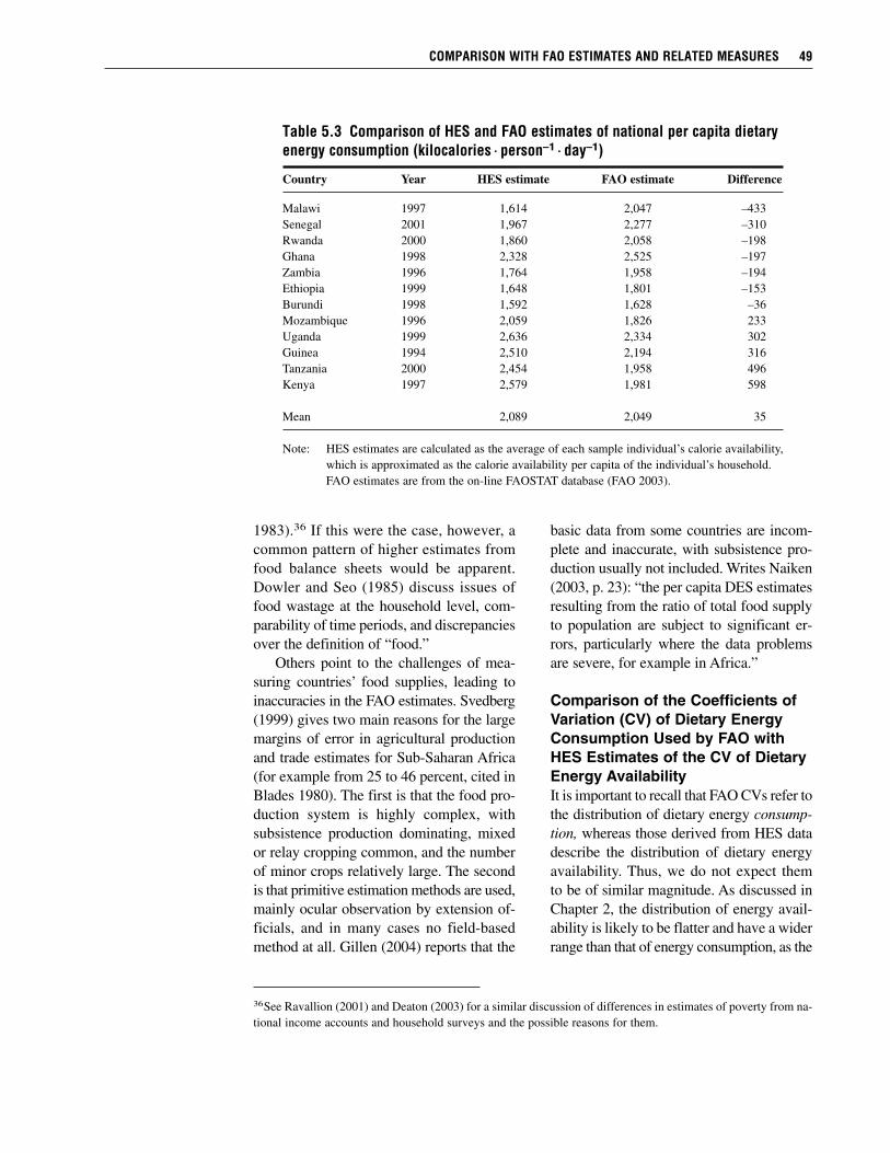
1983).36 If this were the case, however, acommon pattern of higher estimates fromfood balance sheets would be apparent.Dowler and Seo (1985) discuss issues offood wastage at the household level, com-parability of time periods, and discrepanciesover the definition of “food.”
Others point to the challenges of mea-suring countries’ food supplies, leading toinaccuracies in the FAO estimates. Svedberg(1999) gives two main reasons for the largemargins of error in agricultural productionand trade estimates for Sub-Saharan Africa(for example from 25 to 46 percent, cited inBlades 1980). The first is that the food pro-duction system is highly complex, withsubsistence production dominating, mixedor relay cropping common, and the numberof minor crops relatively large. The secondis that primitive estimation methods are used,mainly ocular observation by extension of-ficials, and in many cases no field-basedmethod at all. Gillen (2004) reports that the
basic data from some countries are incom-plete and inaccurate, with subsistence pro-duction usually not included. Writes Naiken(2003, p. 23): “the per capita DES estimatesresulting from the ratio of total food supplyto population are subject to significant er-rors, particularly where the data problemsare severe, for example in Africa.”
Comparison of the Coefficients ofVariation (CV) of Dietary EnergyConsumption Used by FAO withHES Estimates of the CV of DietaryEnergy AvailabilityIt is important to recall that FAO CVs refer tothe distribution of dietary energy consump-tion, whereas those derived from HES datadescribe the distribution of dietary energyavailability. Thus, we do not expect themto be of similar magnitude. As discussed inChapter 2, the distribution of energy avail-ability is likely to be flatter and have a widerrange than that of energy consumption, as the
COMPARISON WITH FAO ESTIMATES AND RELATED MEASURES 49
36See Ravallion (2001) and Deaton (2003) for a similar discussion of differences in estimates of poverty from na-tional income accounts and household surveys and the possible reasons for them.
Table 5.3 Comparison of HES and FAO estimates of national per capita dietaryenergy consumption (kilocalories ⋅⋅ person–1 ⋅⋅ day–1)
Country Year HES estimate FAO estimate Difference
Malawi 1997 1,614 2,047 –433Senegal 2001 1,967 2,277 –310Rwanda 2000 1,860 2,058 –198Ghana 1998 2,328 2,525 –197Zambia 1996 1,764 1,958 –194Ethiopia 1999 1,648 1,801 –153Burundi 1998 1,592 1,628 –36Mozambique 1996 2,059 1,826 233Uganda 1999 2,636 2,334 302Guinea 1994 2,510 2,194 316Tanzania 2000 2,454 1,958 496Kenya 1997 2,579 1,981 598
Mean 2,089 2,049 35
Note: HES estimates are calculated as the average of each sample individual’s calorie availability,which is approximated as the calorie availability per capita of the individual’s household.FAO estimates are from the on-line FAOSTAT database (FAO 2003).
latter conforms to human biological energyintake limits. Its CV is thus expected to behigher.
The main source of distributional datafrom which estimation of FAO CVs startsis HES data on household per capita calorieavailability. FAO has determined that “con-siderable problems are encountered inusing such data for estimating the distribu-tion of dietary energy consumption” (Naiken2003, p. 11). The reliability issues discussedin Chapter 2 are raised, for example, mea-surement errors caused by recall bias, theinclusion of food given to guests and visi-tors and waste, the difficulties of determin-ing the energy content of food consumedaway from home, and the use of shorter-than-annual reference periods for food datacollection, which can inflate variability inthe data.
To overcome the above problems, meanhousehold energy availability per capita forlarge groups of households classified byhousehold per capita income (or total expen-diture) is used. Such a method is believed toprovide reliable estimates of annual averageconsumption to calculate the “CV of house-hold per capita usual dietary energy con-sumption owing to income.” A factor of 0.2is added to account for the variation in di-etary energy requirements. However, for themajority of countries, the data for estimatingthe CV owing to income are not available.When the data are not available, two othertechniques are used. When only data on in-come distribution are available, the param-eter describing the distribution of dietaryenergy is estimated using a cross-countryregression with per capita Gross DomesticProduct as the predictor. For countries forwhich no distributional data are available at
all, the CVs are predicted using data on in-fant mortality rates (Naiken 2003).
Finally, a limit is set on the possibleminimum and maximum CV of 0.2 to 0.35.This range is based on the standard devia-tion of the energy requirement distributionof a hypothetical well-fed population (660kilocalories) and the highest and lowestdeveloping-country dietary energy suppliesper capita (1,900 and 3,400). It is supportedby an analysis of variance of data fromhousehold food consumption surveys con-ducted for small, rural, homogeneous pop-ulations of Bangladesh, Kenya, Pakistan,Philippines, and Zambia.37 Note that ananalysis conducted by FAO shows that theCV in this range makes little differenceto the estimates of food energy deficiency(FAO 1996).
There is some reason to believe that theFAO CVs may be biased downward, forthe following reasons. The true variabilityof food consumption found in developingcountries, where many people fall belowtheir energy requirements and more andmore are falling above, is likely to be higherthan that of a group of people who are justmeeting their requirements. Further, thenational CVs for entire countries are likelyto be higher than those found in a relativelyhomogeneous subnational population (Smith1998a).
Table 5.4 reports energy availability CVsderived from the HES data sets38 and energyconsumption CVs used in the FAO compu-tations. Note that it is not possible to correctfor the sampling design in estimating thestandard deviation from HESs, and thus theCV. The HES-derived CVs presented hereare thus not design unbiased.39 They rangefrom a low of 0.39 for Ethiopia to a high of
50 CHAPTER 5
37These surveys, conducted by IFPRI, are described in more detail in Chapter 2.
38Although they are based on mean household energy availability per capita and its standard deviation, when in-dividual data are used roughly the same estimates are obtained.
39This does not place any limitation on the estimation of food energy deficiency prevalences using the nonpara-metric approach of this report, however, in which a sampling design–corrected proportion is calculated directlyfrom the data without the need for estimating a CV first (as is necessary in the parametric approach).
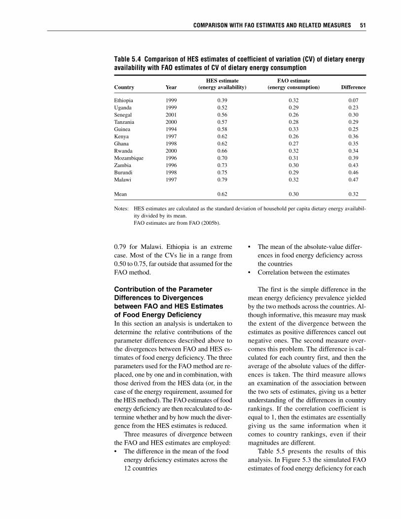
0.79 for Malawi. Ethiopia is an extremecase. Most of the CVs lie in a range from0.50 to 0.75, far outside that assumed for theFAO method.
Contribution of the ParameterDifferences to Divergencesbetween FAO and HES Estimates of Food Energy DeficiencyIn this section an analysis is undertaken todetermine the relative contributions of theparameter differences described above tothe divergences between FAO and HES es-timates of food energy deficiency. The threeparameters used for the FAO method are re-placed, one by one and in combination, withthose derived from the HES data (or, in thecase of the energy requirement, assumed forthe HES method). The FAO estimates of foodenergy deficiency are then recalculated to de-termine whether and by how much the diver-gence from the HES estimates is reduced.
Three measures of divergence betweenthe FAO and HES estimates are employed:• The difference in the mean of the food
energy deficiency estimates across the12 countries
• The mean of the absolute-value differ-ences in food energy deficiency acrossthe countries
• Correlation between the estimates
The first is the simple difference in themean energy deficiency prevalence yieldedby the two methods across the countries. Al-though informative, this measure may maskthe extent of the divergence between theestimates as positive differences cancel outnegative ones. The second measure over-comes this problem. The difference is cal-culated for each country first, and then theaverage of the absolute values of the differ-ences is taken. The third measure allowsan examination of the association betweenthe two sets of estimates, giving us a betterunderstanding of the differences in countryrankings. If the correlation coefficient isequal to 1, then the estimates are essentiallygiving us the same information when itcomes to country rankings, even if theirmagnitudes are different.
Table 5.5 presents the results of thisanalysis. In Figure 5.3 the simulated FAOestimates of food energy deficiency for each
COMPARISON WITH FAO ESTIMATES AND RELATED MEASURES 51
Table 5.4 Comparison of HES estimates of coefficient of variation (CV) of dietary energyavailability with FAO estimates of CV of dietary energy consumption
HES estimate FAO estimateCountry Year (energy availability) (energy consumption) Difference
Ethiopia 1999 0.39 0.32 0.07Uganda 1999 0.52 0.29 0.23Senegal 2001 0.56 0.26 0.30Tanzania 2000 0.57 0.28 0.29Guinea 1994 0.58 0.33 0.25Kenya 1997 0.62 0.26 0.36Ghana 1998 0.62 0.27 0.35Rwanda 2000 0.66 0.32 0.34Mozambique 1996 0.70 0.31 0.39Zambia 1996 0.73 0.30 0.43Burundi 1998 0.75 0.29 0.46Malawi 1997 0.79 0.32 0.47
Mean 0.62 0.30 0.32
Notes: HES estimates are calculated as the standard deviation of household per capita dietary energy availabil-ity divided by its mean.FAO estimates are from FAO (2005b).

country are compared with the HES esti-mates under the various parameterizations.The baseline difference between the meansof the HES and FAO estimates is 19.5 per-centage points (58.5% vs. 39%) (Table 5.5,column 1 and Fig. 5.3A). The mean of theabsolute value differences across the 12countries is 20. The correlation coefficientis 0.46 and is not statistically significant.
When the FAO estimates are recalculatedusing the average energy requirements forlight activity assumed for the HES methodinstead of the minimum requirements, theyincrease substantially (Fig. 5.3B). The meanfood energy deficiency prevalence rises from39 percent to 56 percent, giving a differencein means of 2.8 percentage points (Table 5.5,column 2). Concurrently, the mean absolutevalue difference between the HES and FAOestimates drops from 20 to 11.7 percentagepoints. Further, the correlation between theestimates rises from 0.46 to 0.56, becom-ing statistically significant at the 10 percentlevel. We can thus conclude that some of the
country-level differences between the HESand FAO estimates can be attributed to theuse of a lower set of dietary energy require-ments for the latter, which lowers the per-centage of people considered to be foodenergy deficient. It is important to note,however, that quite a large divergence re-mains, with the differences between the esti-mates being far from zero and their correla-tion far from perfect. This means that muchof the divergence remains to be explainedby differences in the other two parameters.
In regard to mean dietary energy con-sumption, column 3 of Table 5.5 shows thatthe major HES–FAO differences in thisparameter described above (see Table 5.1)translate into a large contribution to diver-gences in estimates of food energy avail-ability. When the original FAO parameter isreplaced with that derived from HESs, thereis only a slight reduction in the mean differ-ences measures. However, the correlationbetween the FAO and HES estimates risesfrom 0.46 to 0.98, or almost 1.0. These re-
52 CHAPTER 5
Table 5.5 Differences and correlations between FAO and HES estimates of food energy deficiency when FAOestimates are recalculated using HES parameters
Recalculation of FAO estimates using:
HES requirement and
HES mean HES MeanOriginal dietary coefficient dietary
FAO HES energy of energy Coefficient All HESestimates requirement consumption variation consumption of variation parameters
Measure (1) (2) (3) (4) (5) (6) (7)
Difference between HES and 19.5 2.8 18.3 6.0 4.4 –2.7 –1.6FAO estimate means across countries (percentage points)
Mean of country-level absolute 20.0 11.7 18.3 10.9 9.4 9.0 1.7value differences between HES and FAO estimates (percentage points)
Pearson correlation coefficient 0.456 0.558 0.981 0.569 0.987 0.643 0.997between HES and FAO estimates
(P = 0.136) (P = 0.059) (P = 0.000) (P = 0.054) (P = 0.000) (P = 0.024) (P = 0.000)
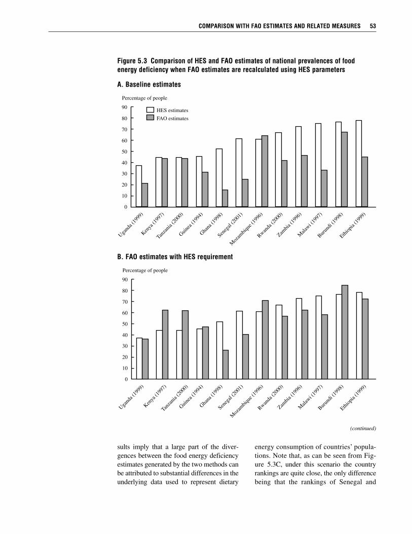
sults imply that a large part of the diver-gences between the food energy deficiencyestimates generated by the two methods canbe attributed to substantial differences in theunderlying data used to represent dietary
energy consumption of countries’ popula-tions. Note that, as can be seen from Fig-ure 5.3C, under this scenario the countryrankings are quite close, the only differencebeing that the rankings of Senegal and
COMPARISON WITH FAO ESTIMATES AND RELATED MEASURES 53
Figure 5.3 Comparison of HES and FAO estimates of national prevalences of foodenergy deficiency when FAO estimates are recalculated using HES parameters
A. Baseline estimates
B. FAO estimates with HES requirement
(continued)

Mozambique, and of Burundi and Ethiopia,are reversed.
With respect to the third parameter, theCV, when the FAO estimates of this param-eter are replaced with those derived fromHESs, FAO estimates of food energy defi-ciency increase for all 12 of the study coun-
tries. The mean absolute value differencebetween the FAO and HES estimates de-creases from 20 to 10.9 percentage points;their correlation increases somewhat, from0.46 to 0.57 (Table 5.5, column 4).
We can learn more about the relativecontributions of the mean and CV by assum-
54 CHAPTER 5
Figure 5.3—Continued
C. FAO estimates with HES mean dietary energy consumption
D. FAO estimates with HES coefficient of variation in dietary energy availability

ing that the energy requirements are the same(the average requirement) and then seeingwhat happens when these two other param-eters are replaced, one at a time, by theirHES equivalents. This is an interesting ex-
periment in that the requirements are as-sumed, whereas the other parameters areestimated using different methods and data.Column 5 of Table 5.5 (and Fig. 5.3E) showswhat happens when the FAO estimates are
COMPARISON WITH FAO ESTIMATES AND RELATED MEASURES 55
Figure 5.3—Continued
E. FAO estimates with HES requirement and mean dietary energy consumption
F. FAO estimates with HES requirement and coefficient of variation in dietary energyavailability
(continued)
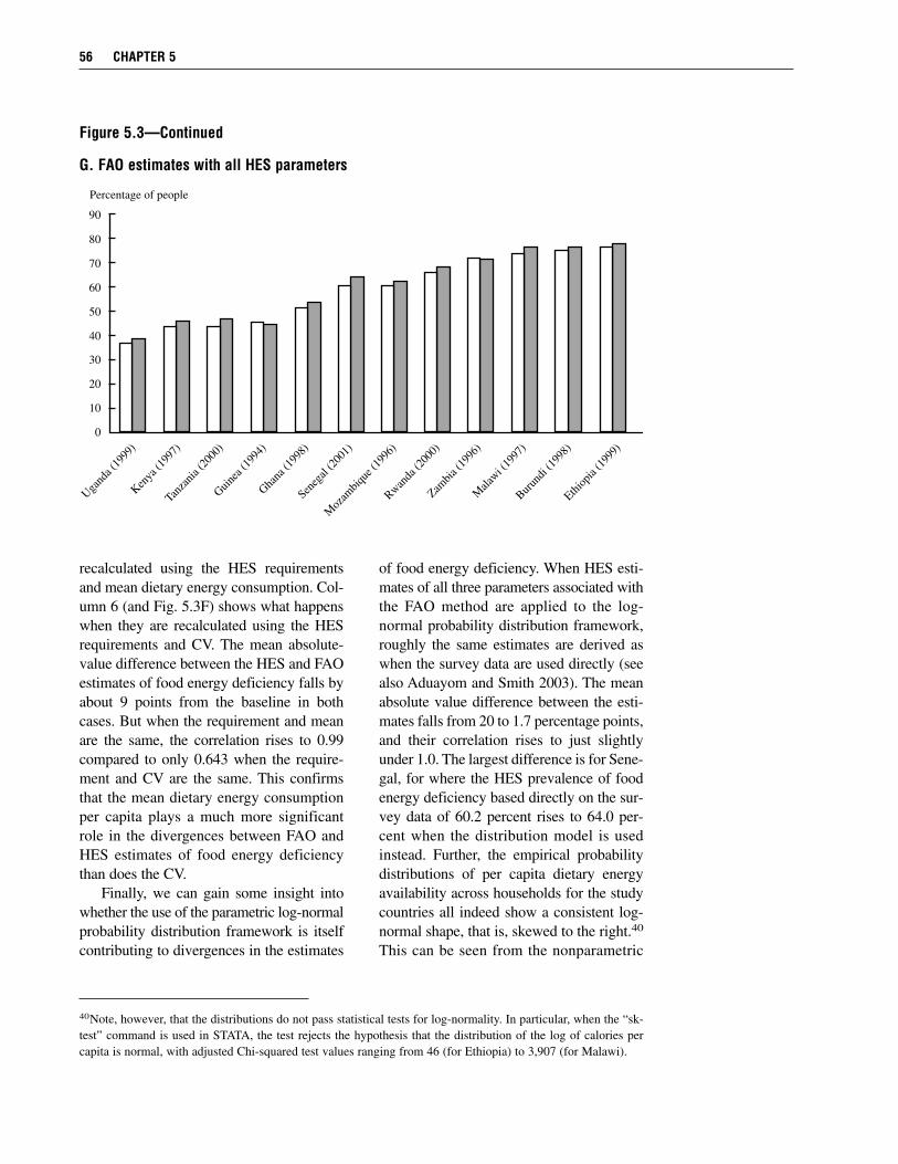
recalculated using the HES requirementsand mean dietary energy consumption. Col-umn 6 (and Fig. 5.3F) shows what happenswhen they are recalculated using the HESrequirements and CV. The mean absolute-value difference between the HES and FAOestimates of food energy deficiency falls byabout 9 points from the baseline in bothcases. But when the requirement and meanare the same, the correlation rises to 0.99compared to only 0.643 when the require-ment and CV are the same. This confirmsthat the mean dietary energy consumptionper capita plays a much more significantrole in the divergences between FAO andHES estimates of food energy deficiencythan does the CV.
Finally, we can gain some insight intowhether the use of the parametric log-normalprobability distribution framework is itselfcontributing to divergences in the estimates
of food energy deficiency. When HES esti-mates of all three parameters associated withthe FAO method are applied to the log-normal probability distribution framework,roughly the same estimates are derived aswhen the survey data are used directly (seealso Aduayom and Smith 2003). The meanabsolute value difference between the esti-mates falls from 20 to 1.7 percentage points,and their correlation rises to just slightlyunder 1.0. The largest difference is for Sene-gal, for where the HES prevalence of foodenergy deficiency based directly on the sur-vey data of 60.2 percent rises to 64.0 per-cent when the distribution model is usedinstead. Further, the empirical probabilitydistributions of per capita dietary energyavailability across households for the studycountries all indeed show a consistent log-normal shape, that is, skewed to the right.40
This can be seen from the nonparametric
56 CHAPTER 5
40Note, however, that the distributions do not pass statistical tests for log-normality. In particular, when the “sk-test” command is used in STATA, the test rejects the hypothesis that the distribution of the log of calories percapita is normal, with adjusted Chi-squared test values ranging from 46 (for Ethiopia) to 3,907 (for Malawi).
Figure 5.3—Continued
G. FAO estimates with all HES parameters

probability density functions of Figure 3.2in Chapter 3 and indicates that the distribu-tion of calorie consumption are log-normalas well. These findings suggest that use ofa theoretical probability distribution frame-work in general, and of the log-normal as-sumption in particular, is not a major factordriving the discrepancies in the HES andFAO estimates of food energy deficiency.
In sum, the analysis of this section hasshown that it is not the FAO method itselfthat underlies divergences in the FAO andHES estimates of food energy deficiency butinstead differences in the underlying param-eters used. The mean of the absolute-valuedifferences across the countries is a summarymeasure of the distance between the twoestimates in terms of direct comparisons oflevels. From this perspective the differenceis reduced the most, but only by just overhalf, when the CVs and energy requirementsare the same. The correlation coefficient isa summary measure of the degree of asso-ciation between the two measures. The con-cern here is with both levels and countryrankings, which are equally important forpolicy purposes. The correlation betweenthe measures under the different parameter-
izations (first three scenarios) rises the mostwhen mean household dietary energy con-sumption is equalized, almost to 100 per-cent agreement. It rises only slightly whenthe energy requirements and CVs are equal-ized. This suggests that the most importantfactors underlying the differences betweenHES and FAO estimates of food energy de-ficiency for Sub-Saharan African countriesare the implied estimates of food consump-tion in countries.
Comparison of HES and FAOEstimates with Poverty andChild MalnutritionOne way to determine whether HES data canbe used to improve the accuracy of FAO es-timates of food energy deficiency is to inves-tigate how both compare to other indicatorsthat are related to food security and that arewidely believed to be accurately measured.Table 5.6 gives estimates of poverty, whichis a primary determinant of food security,and child malnutrition, of which food se-curity is in turn a major determinant, for thecountries and time periods for which theyare available. Both of these measures are
COMPARISON WITH FAO ESTIMATES AND RELATED MEASURES 57
Table 5.6 Poverty and child malnutrition prevalences for study countries
Poverty Child malnutrition(<< US$1 per day) (underweight)
Country Year (%) (%)
Burundi 1998 58.4 45.1Ethiopia 1999 81.9 47.2Ghana 1998 44.8 24.9Guinea 1994Kenya 1997 23.0 22.1Malawi 1997 41.7 29.6Mozambique 1996 37.9 26.1Rwanda 2000 24.3Senegal 2001 22.7Tanzania 2000 29.4Uganda 1999 22.8Zambia 1996 63.7 23.5
Notes: Poverty estimates are from World Bank (2003). Child malnutrition estimates arefrom WHO (2003). They are from surveys undertaken within 2 years of the HESsurveys under study in this report.

conceptually close to, yet still distinct from,food insecurity (see Fig. 2.1 in Chapter 2).Thus, although we would expect some pos-itive correlation between them and a measureof food insecurity, we would not expect anexact correlation. The poverty estimates arereported by the World Bank (2003) and rep-resent the percentage of countries’ popula-tions that live on less than US$1 per day.They are available for only seven of thecountries. Note that some of the correlationbetween the poverty and food energy defi-ciency estimates can be attributed to the useof the same data sources as well as to con-ceptual closeness of the indicators. The childmalnutrition estimates are from WHO (2003)and represent the percentage of children lessthan 5 years old who are underweight fortheir age. They are available for all countriesexcept Guinea. Figure 5.4 compares the HESfood energy deficiency and poverty esti-mates. Their Pearson correlation coefficient,reported in Table 5.6, is 0.78 (P = 0.039).Figure 5.5 compares the HES food energydeficiency and child malnutrition preva-lences. Here the association is less strong,but still significant. The Pearson correlationcoefficient is 0.60 (P = 0.053).
Table 5.7 also gives correlation coeffi-cients between poverty and child malnutri-tion and FAO estimates of food energy defi-ciency prevalence. The Pearson correlation,at 0.12, is far lower than that for the HESestimates and is not statistically significant.The child malnutrition correlation, also sta-tistically insignificant, is somewhat lowerthan the HES correlation. Spearman rankcorrelations are also given in Table 5.7. Herethe divergence between the correlations withchild malnutrition is greater, with that forthe HES estimates being 0.68 (P = 0.022)and that for the FAO estimates being 0.41and not significant. Evidently, the HES esti-mates are more strongly associated withpoverty and child malnutrition when it comesto both magnitudes and country rankings.
Comparison of HES and FAOEstimates with CountryRankings from a Survey of Expert OpinionThere is no gold standard with which tojudge the accuracy of estimates of foodenergy deficiency. However, a potentiallyuseful way to judge them is to rely on the
58 CHAPTER 5
Figure 5.4 Comparison of HES estimates of national prevalences of food energydeficiency with poverty
Source: See Table 6.3.
90
80
70
60
50
40
30
20
10
0Kenya(1997)
Ghana(1998)
Mozambique(1996)
Zambia(1996)
Malawi(1997)
Burundi(1998)
Ethiopia(1999)
HES estimates of food energy deficiency
Poverty
Percentage of people food energy deficient
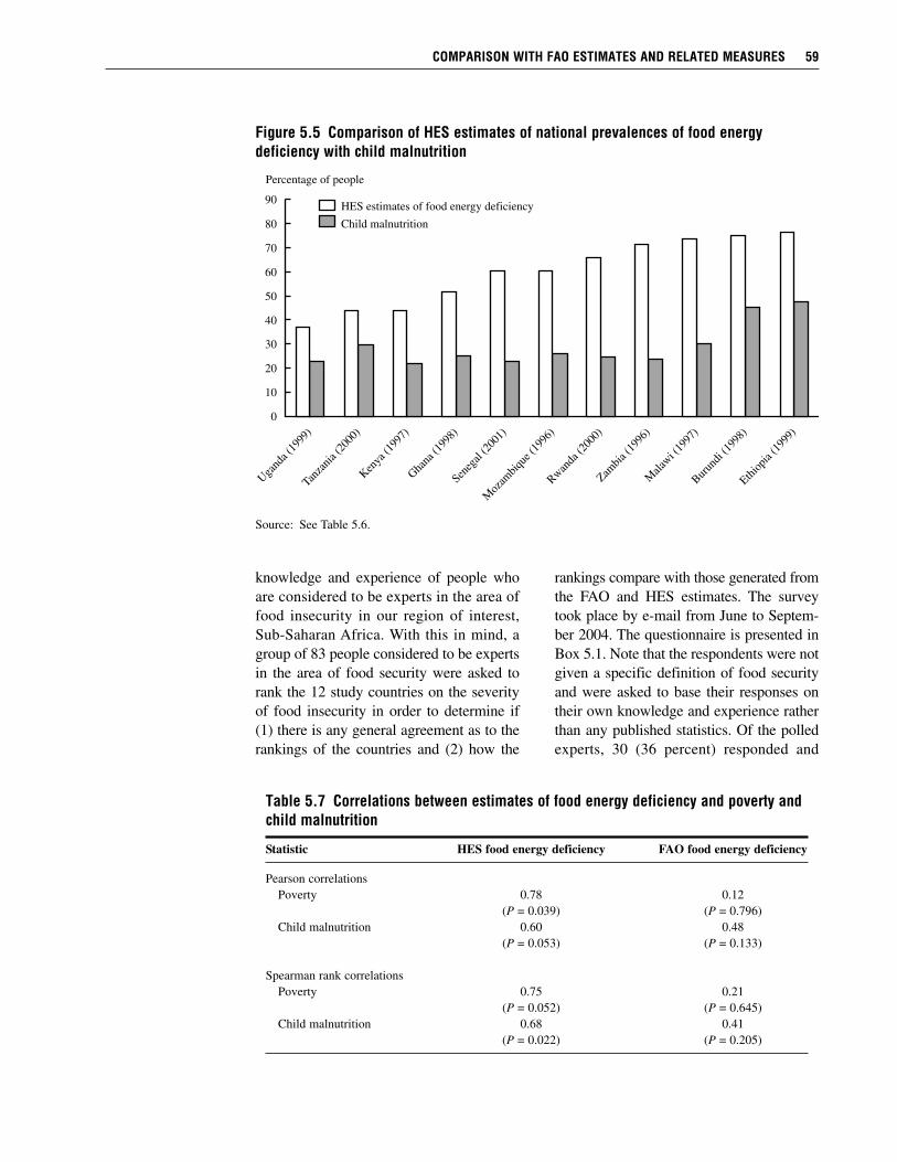
knowledge and experience of people whoare considered to be experts in the area offood insecurity in our region of interest,Sub-Saharan Africa. With this in mind, agroup of 83 people considered to be expertsin the area of food security were asked torank the 12 study countries on the severityof food insecurity in order to determine if(1) there is any general agreement as to therankings of the countries and (2) how the
rankings compare with those generated fromthe FAO and HES estimates. The surveytook place by e-mail from June to Septem-ber 2004. The questionnaire is presented inBox 5.1. Note that the respondents were notgiven a specific definition of food securityand were asked to base their responses ontheir own knowledge and experience ratherthan any published statistics. Of the polledexperts, 30 (36 percent) responded and
COMPARISON WITH FAO ESTIMATES AND RELATED MEASURES 59
Figure 5.5 Comparison of HES estimates of national prevalences of food energydeficiency with child malnutrition
Source: See Table 5.6.
Table 5.7 Correlations between estimates of food energy deficiency and poverty andchild malnutrition
Statistic HES food energy deficiency FAO food energy deficiency
Pearson correlationsPoverty 0.78 0.12
(P = 0.039) (P = 0.796)Child malnutrition 0.60 0.48
(P = 0.053) (P = 0.133)
Spearman rank correlationsPoverty 0.75 0.21
(P = 0.052) (P = 0.645)Child malnutrition 0.68 0.41
(P = 0.022) (P = 0.205)

ranked the countries. Nine refused to rankthe countries, and 46 did not respond. Theinstitutional affiliations of the respondentsare as follows:• Nongovernmental development
assistance agencies (4)• Governmental development assistance
and United Nations agencies (3)• Development technical assistance
agencies (6)• Research and academia (15)• Foundations (2)
An average rank score based on theresponses was calculated for each country,resulting in the ranking presented in Table5.8.41 To get a sense of whether the respon-dents agreed with one another, the table re-ports the number who rated each country 1,2, and so forth. The number of respondentswho ranked the country in the final meanrank position is highlighted along the matrixdiagonal. In no case did all of the respon-dents rank a country the same. At the ex-tremes of the final rank (ranks 1, 2, 3, and
60 CHAPTER 5
41Six respondents ranked fewer than 12 countries (from 8 to 11) citing insufficient personal knowledge about theomitted countries. In order to render these respondents’ responses comparable to the others, their raw scores wereadjusted by multiplying the given rank by a factor of 12 divided by the number of countries ranked before com-puting the average rank score for all respondents.
Box 5.1 Expert Opinion Survey on Food Insecurity in Study Countries: Questionnaire
Greetings,You have been referred to me as a person who has broad knowledge of the food se-
curity situation in Sub-Saharan African countries. Could you take a few moments to rankthe following 12 countries on the severity of food insecurity in the mid- to late 1990s(starting with most severe to least severe food insecurity)? Please base your ranking onyour own knowledge and experience.
Feel free to leave out countries and make qualifying comments at your discretion.
BurundiEthiopiaGhanaGuineaKenyaMalawiMozambiqueRwandaSenegalTanzaniaUgandaZambia
Thank you for your time. If you have suggestions of others who could undertake thisranking, I would appreciate your sending me their names.
Lisa SmithResearch FellowInternational Food Policy Research Institute

11 and 12), there is generally more agree-ment than in the middle. Ethiopia is the coun-try for whom there was the most agreement,with 70 percent of respondents ranking it ashaving the most severe food insecurity.
A kappa test statistic of interrater agree-ment was calculated for each of the 12 pos-sible ranks and for overall agreementamong the respondents (StataCorp 2003).The statistic ranges from 0 to 1, with thefollowing interpretations on the degree ofagreement (Landis and Koch 1977):
0 Expected by chance>0 to 0.20 Slight0.21–0.40 Fair0.41–0.60 Moderate0.61–0.81 Substantial0.81–1.00 Almost perfect
The only country for which even mod-erate agreement was found is Ethiopia, forwhom the test statistic is 0.526. The rank-ings for Uganda and Ghana (11 and 12) ex-hibited “slight” agreement, that for Malawi(2) exhibited “fair” agreement, and the rank-ings for the remaining countries exhibited“poor” agreement. The overall test statisticis 0.113, signaling only slight agreement.
Clearly, the rankings of the experts do notrepresent a consensus. This could be a re-sult of differing definitions of the conceptof food insecurity, different sources of in-formation, different evaluation criteria, vari-ation in temporal frame of reference, anddiffering degrees of knowledge of the foodsecurity situations in the countries.
Table 5.9 compares the average expertopinion survey rankings to those derivedfrom FAO and HES estimates of food en-ergy deficiency. In no case is any one coun-try ranked exactly the same by all threecriteria. The countries for which there isthe most disagreement are Tanzania andKenya. The countries for which there isthe most agreement are Burundi, Rwanda,Guinea, and Uganda. Note that the FAOestimate rankings are more similar to theexperts’ ranking at the bottom end of thescale, whereas HES ranks are more similarto them at the top of the scale.
Table 5.10 presents the results of twotests for agreement between the averageexpert survey ranking on the one hand andthe FAO and HES rankings on the other.The Spearman correlation between theexpert ranking and the HES ranking is0.83, whereas that for the FAO ranking
COMPARISON WITH FAO ESTIMATES AND RELATED MEASURES 61
Table 5.8 Expert opinion survey: Respondent rankings
Respondent rankings
Average Number ofCountry rank 1 2 3 4 5 6 7 8 9 10 11 12 rankings
Ethiopia 1 21 5 2 1 1 30
Malawi 2 1 15 6 2 1 1 1 2 29
Burundi 3 2 4 6 3 3 5 3 3 1 30
Mozambique 4 3 8 4 6 3 3 2 29
Rwanda 5 2 2 5 6 3 5 3 4 30
Zambia 6 1 3 3 6 3 2 3 2 1 3 1 28
Guinea 7 1 3 2 2 5 3 2 3 3 2 26
Tanzania 8 3 1 3 7 7 1 3 4 1 30
Kenya 9 4 3 2 5 1 8 5 2 30
Senegal 10 3 1 1 2 4 3 7 6 27
Uganda 11 1 2 2 9 3 6 7 30
Ghana 12 1 1 3 2 2 11 8 28
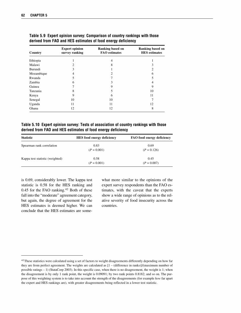
is 0.69, considerably lower. The kappa teststatistic is 0.58 for the HES ranking and0.45 for the FAO ranking.42 Both of thesefall into the “moderate” agreement category,but again, the degree of agreement for theHES estimates is deemed higher. We canconclude that the HES estimates are some-
what more similar to the opinions of theexpert survey respondents than the FAO es-timates, with the caveat that the expertsshow a wide range of opinions as to the rel-ative severity of food insecurity across thecountries.
62 CHAPTER 5
42These statistics were calculated using a set of factors to weight disagreements differently depending on how farthey are from perfect agreement. The weights are calculated as [1 – (difference in ranks)]/(maximum number ofpossible ratings – 1) (StataCorp 2003). In this specific case, when there is no disagreement, the weight is 1; whenthe disagreement is by only 1 rank point, the weight is 0.09091; by two rank points 0.8182; and so on. The pur-pose of this weighting system is to take into account the strength of the disagreements (for example how far apartthe expert and HES rankings are), with greater disagreements being reflected in a lower test statistic.
Table 5.9 Expert opinion survey: Comparison of country rankings with thosederived from FAO and HES estimates of food energy deficiency
Expert opinion Ranking based on Ranking based onCountry survey ranking FAO estimates HES estimates
Ethiopia 1 4 1Malawi 2 8 3Burundi 3 1 2Mozambique 4 2 6Rwanda 5 7 5Zambia 6 3 4Guinea 7 9 9Tanzania 8 5 10Kenya 9 6 11Senegal 10 10 7Uganda 11 11 12Ghana 12 12 8
Table 5.10 Expert opinion survey: Tests of association of country rankings with thosederived from FAO and HES estimates of food energy deficiency
Statistic HES food energy deficiency FAO food energy deficiency
Spearman rank correlation 0.83 0.69(P = 0.001) (P = 0.126)
Kappa test statistic (weighted) 0.58 0.45(P = 0.001) (P = 0.007)

C H A P T E R 6
Evidence on Cross-Country Comparabilityand Other Reliability Issues
Cross-Country Comparability
The data cleaning, processing, and computation protocols employed for this researchare standard for all countries (see Chapter 3). However, differences in data collectionmethodologies raise some issues of cross-country comparability. In this chapter we use
the country-level estimates from the surveys used in this report to gain some insights.Table 6.1 compares the diet quantity and quality estimates across groups of the surveyed
countries with similar data collection methods on the following characteristics:• Recall period (less or greater than 1 week)• Reference period (1–2 weeks versus 2 weeks to 1 month versus 1 month)• Number of food items for which data were collected (less or greater than 110)• Means of data collection (interview or diary)• Whether in-kind food acquisitions are included
These characteristics are specified for each country in Table 3.2 in Chapter 3.With respect to the first characteristic, the recall period, the discussion in Chapter 2 pointed
to the possibility that a longer recall period would lead to a greater chance of recall bias, thatis, lower reporting of food quantities or expenditures because of memory failure. On the otherhand, a shorter recall period may lead to telescoping, where the respondent includes eventsthat occur before the recall period, thus inflating estimates of food acquisition. In the case ofthe diet quantity measures, Table 6.1 shows little difference across the groups of countries witha recall period less than 1 week and greater than 1 week. The difference in energy availabilityper capita is 83 kilocalories; the difference in the percentage of people food energy deficientis 2.8 percentage points. Both differences are not statistically significant. The moderate dif-ferences across the groups for the diet quality measures are not statistically significant.
The length of the survey reference period also appears to make little difference for the dietquantity measures. In particular, the issue raised in Chapter 2 that the length of the referenceperiod influences the dispersion of energy availability and thus the percentage food energy de-ficient does not seem to be a major problem. Although the dispersion is indeed smaller thelonger is the reference period (the CV drops from 0.7 to 0.6 and then 0.5 across the groups),it is apparently not enough to influence the percentage food energy deficient.
The figures reported in Table 6.1 indicate that the reference period may matter, however,for the diet quality measures. As discussed in Chapter 3, the longer the reference period themore variety is picked up simply because people are likely to acquire a wider variety of foodswith the passage of more time. The diet diversity score is 4.6 for the group of countries with
63
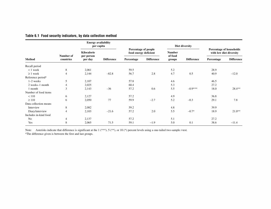
Table 6.1 Food security indicators, by data collection method
Energy availability
Percentage of people Percentage of householdsper capita
food energy deficient
Diet diversity
with low diet diversityKilocalorie NumberNumber of per person of food
Method countries per day Difference Percentage Difference groups Difference Percentage Difference
Recall period< 1 week 8 2,061 59.5 5.2 28.9≥ 1 week 4 2,144 –82.8 56.7 2.8 4.7 0.5 40.9 –12.0
Reference perioda
1–2 weeks 5 2,107 57.8 4.6 46.52 weeks–1 month 4 2,025 60.4 5.3 27.21 month 3 2,143 –36 57.2 0.6 5.5 –0.9*** 18.0 28.4**
Number of food items< 110 6 2,127 57.2 4.9 36.8≥ 110 6 2,050 77 59.9 –2.7 5.2 –0.3 29.1 7.8
Data collection meansInterview 8 2,082 59.2 4.8 39.9Diary/interview 4 2,103 –21.6 57.2 2.0 5.5 –0.7* 18.9 21.0**
Includes in-kind foodNo 4 2,137 57.2 5.1 27.2Yes 8 2,065 71.5 59.1 –1.9 5.0 0.1 38.6 –11.4
Note: Asterisks indicate that difference is significant at the 1 (***), 5 (**), or 10 (*) percent levels using a one-tailed two-sample t-test.aThe difference given is between the first and last groups.

reference periods of 1–2 weeks. It rises to5.5 for those with reference periods of 1month. The percentage of households witha low-quality diet falls from 47 percent to18 percent. Both of these differences arestatistically significant.
To investigate this issue further, a 1-week-equivalent adjustment factor wasapplied to the country-level estimates as fol-lows. First, an Ordinary Least Squares re-gression equation was run using the datafrom all households included in the studydata sets except Malawi and Zambia (n =97,292).43 The dependent variable was thenumber of food groups, and the main in-dependent variable was the household-specific reference period, which may differacross households in the survey (see Table3.2).44 The regression yielded a referenceperiod coefficient of 0.017 (t = 12.7, R2 =0.358). For each country the adjustment fac-tor was calculated as the coefficient multi-plied by the difference between the numberof days in the reference period and 7 (or 1week).45 This procedure yielded adjustmentfactors ranging from 0.1 to 0.4 food groups.This analysis suggests that for all practicalpurposes the length of the reference perioddoes not pose major problems of cross-country comparability of estimates of dietdiversity.
Greater specificity and detail in thedelineation of food items in a survey arethought to lead to greater reporting accuracyand higher estimates of food acquisition.
The evidence presented in Table 6.1 doesnot support this supposition. The energyavailability per capita of the countries witha large number of food items is only 77 kilo-calories greater than that of countries with alow number, and the difference is not statis-tically significant. The diet quality measuresalso differ very little across the two groups.
The means of data collection, whetherdiary or interview, appears to have little ef-fect on the diet quantity measures but maymake some difference for diet quality. Dietdiversity is higher for the group of countriesfor which the diary method was employed,by 0.7 food groups, although the differenceis not strongly significant. The percentage ofhouseholds with a low-quality diet is lowerby 21 percentage points, but this differenceis not statistically significant.
Finally, whether the survey includedquestions on households’ acquisition of in-kind food seems to make little difference tothe estimates of the diet quantity and qualitymeasures. For diet quantity, this means thatin-kind food adds little to the overall energyavailable to households. For diet quality, itimplies that in-kind food acquisitions do notsignificantly increase the variety of foodsacquired by households.
These initial findings indicate no majorproblem of comparability across countriesof HES estimates of food energy avail-ability, prevalences of food energy defi-ciency, diet diversity, and prevalences oflow diet diversity.
EVIDENCE ON CROSS-COUNTRY COMPARABILITY 65
43Households from Malawi and Zambia are left out because for these countries the reference period differs forpurchased and nonpurchased foods, making it impossible to assign a single reference period to each household.
44Other variables controlled for were the number of household adult equivalents, variables representing theage–sex composition of the household, whether it is female headed, age of the household head, whether at leastone adult member has a primary or secondary education, country of residence, and urban or rural location. It isespecially important to control for the latter because the reference period differs across urban and rural areas forthree of the surveys (Guinea, Rwanda, and Senegal).
45For the three surveys with differences in the reference period by urban and rural area (Guinea, Rwanda, andSenegal), the adjustment factor is applied to the diet diversity measure separately for the areas, and then the ad-justed national measure is calculated as a weighted average of the urban and rural estimates, with the populationproportions in each area as weights. For Zambia, the reference period used is 14 days (only maize purchases havethe higher reference period of 30 days). For Malawi, the reference period used is 12 days, which is the averagehousehold-level reference period over all food acquisitions, whether purchased or nonpurchased.

The Appropriateness of Applying EnergyRequirements at theHousehold LevelThe dietary energy requirements reportedin FAO/WHO/UNU (1985) and used inthis report refer to the average requirementsfor people of different age and sex groupsperforming light activity. As discussed inChapter 2, there is a range of requirementsconsistent with good health and this activitylevel within an age–sex group, depending onindividuals’ body weights, genetic makeup,and so on. Thus, it is inappropriate to applythe requirements to any particular individ-ual to judge whether she or he is consumingadequate dietary energy. By inference, it isalso inappropriate to apply the requirementsat the household level. Thus, the require-ments are recommended to be applied topopulation groups rather than individualsor households. Yet with the nonparametricmethod of this report, they are applied di-rectly at the household level before an esti-
66 CHAPTER 6
Table 6.2 Comparison of national prevalences of food energy deficiency estimated withenergy requirements applied at the household and national levels
Energy Energyrequirements requirementsapplied at the applied at the
household level national level DifferenceCountry Year (%) (%) (percentage points)
Ethiopia 1999 76.4 77 –0.6Burundi 1998 74.8 76 –1.2Malawi 1997 73.3 76 –2.7Zambia 1996 71.1 71 0.1Rwanda 2000 65.3 68 –2.7Mozambique 1996 60.3 62 –1.7Senegal 2001 60.2 64 –3.8Ghana 1998 51.4 53 –1.6Guinea 1994 45.1 45 0.1Kenya 1997 43.9 46 –2.1Tanzania 2000 43.9 47 –3.1Uganda 1999 36.8 39 –2.2
Mean 58.5 60.2 –1.7
Note: Estimates using energy requirements applied at the household level are from Table 4.1. Estimates usingenergy requirements applied at the national level are simulated assuming the log-normal probability dis-tribution model.
mate is made of the percentage of peoplewho are food energy deficient in a country.This raises concern about the reliability ofthe estimates generating using this method.
To investigate whether the method isvalid for estimating national food energydeficiency prevalences given the above con-cern, we can compare the prevalences gen-erated with those generated using the log-normal probability distribution model (seeChapter 5), for which a requirement can beapplied at the population group level. Themean and coefficient of variation (CV) de-rived from the HES data (see Tables 5.3 and5.4) and the national per capita dietary en-ergy requirements given in Table 5.2 areapplied. Table 6.2 compares food energydeficiency prevalences derived using thetwo approaches for the 12 study countries.The mean difference between the estimatesis –1.7 percentage points, signaling a slighttendency for the prevalence to be lower whenthe requirement is applied at the householdlevel. However, the difference is minimal,

with the largest being –3.8 percentage pointsfor Senegal. These results suggest that ap-plication of the energy requirements at thehousehold level is not an obstacle to esti-mating national prevalences of food energydeficiency using the nonparametric approachfollowed in this report.
Sensitivity of Estimates ofFood Energy Deficiency tothe Coefficient of VariationIn Chapter 2, the possibility was discussedthat CVs of dietary energy availability esti-mated using HES data are upward biased,thus biasing estimates of food energy defi-ciency. The reasons for the bias are (1) theinevitable presence of nonsampling errorsin the collection and processing of the dataand (2) the cost-saving use of referenceperiods shorter than 1 year. Given the dataat hand, we cannot determine the magni-tude of this bias. However, we can explorewhether the CV has a large effect on food en-ergy deficiency estimates and country rank-
ings. If not, then the problem of upwardlybiased CVs is not of major concern.
To do so we calculate the prevalence offood energy deficiency at alternative CVs,starting with the original CVs, progressingto a 10 percent lower CV, a 20 percent lowerCV, and then a 30 percent lower CV, againusing the log-normal probability distributionmodel. The estimates of food energy defi-ciency are simulated using the log-normaldistribution framework employed above.Panel A of Table 6.3 gives the estimatesunder the different scenarios, panel B thepercentage difference from the original esti-mates, and panel C the country rankings.
At a 10 percent lower CV, the estimatesof food energy deficiency change very little,with the percentage difference from the orig-inal estimates being the highest for Guinea,at 5.7 percent, and the country rankingschanging (by 1 point) for only two coun-tries, Senegal and Mozambique. At a 20 per-cent lower CV, the changes are somewhatgreater. At a 30 percent lower CV, somefairly substantial changes begin to appear,
EVIDENCE ON CROSS-COUNTRY COMPARABILITY 67
Table 6.3 Prevalences of food energy deficiency at alternative coefficients of variation of dietary energyavailability per capita
HES prevalence of Percent difference fromfood energy deficiency original prevalence Country rankings
(A) (B) (C)
10% 20% 30% 10% 20% 30% 10% 20% 30%lower lower lower lower lower lower lower lower lower
Country Original CV CV CV CV CV CV Original CV CV CV
Uganda 36.8 36 34 32 1.0 8.1 15.8 1 1 1 1Tanzania 43.9 44 42 41 -1.2 3.3 8.0 2 2 3 4Kenya 43.9 44 42 40 0.3 5.3 10.5 3 3 4 3Guinea 45.1 43 41 39 5.7 11.1 16.8 4 4 2 2Ghana 51.4 51 50 48 0.6 3.6 6.7 5 5 5 5Senegal 60.2 63 63 63 –5.0 –4.5 –4.1 6 7 7 7Mozambique 60.3 61 60 60 –1.3 0.0 1.3 7 6 6 6Rwanda 65.3 67 67 67 –2.9 –2.5 –2.3 8 8 8 8Zambia 71.1 71 71 71 0.6 0.7 0.7 9 9 9 9Malawi 73.3 76 76 76 –3.3 –3.6 –3.9 10 10 10 10Burundi 74.8 76 76 76 –1.3 –1.6 –2.0 11 11 11 11Ethiopia 76.4 78 80 81 –2.5 –3.9 –5.3 12 12 12 12
Mean 58.5 59.2 58.4 57.7
with Uganda and Guinea exhibiting thelargest differences from the original esti-mates, at 15.8 percent and 16.8 percent,respectively. The country rankings stay thesame for eight of the countries, but forSenegal and Mozambique they change by1 point, and for Tanzania and Guinea theychange by 2 points.
From this analysis we conclude that theissue of increased variability in estimates ofhousehold calorie availability per capita de-rived from HESs as a result of nonsamplingerrors and short reference periods would bea major concern only if variability, as mea-sured by the coefficient of variation, were tobe upwardly biased by at least 30 percent.
68 CHAPTER 6
C H A P T E R 7
Conclusion
This report has used household expenditure survey (HES) data sets from 12 Sub-SaharanAfrican countries to reach three objectives. The first is to explore the extent and loca-tion of food insecurity within and across the countries. The second is to investigate the
scientific merit of using the food data collected in HESs to measure food insecurity. The thirdis to compare food energy deficiency estimates generated using HES data with those reportedby FAO and begin to explore the reasons for the differences between the two. The study usesboth a diet quantity and a diet quality measure of food insecurity. These are (1) the per-centage of people who consume insufficient dietary energy, or the prevalence of “food energydeficiency,” and (2) the percentage of households with low diet diversity, an indicator of poordiet quality. A household is considered to have low diet diversity if it fails to acquire foodsfrom at least four of seven groups that are sources of essential nutrients for human nutritionalwell-being.
Research Findings and Policy Implications
Extent and Location of Food InsecurityThis study confirms that food insecurity is a major problem in Sub-Saharan Africa. The low-est prevalence of food energy deficiency found at the country level is 37 percent, for Uganda.Even in this country more than one-third of all people do not have access to sufficient food tomeet their energy requirements for light activity. The prevalence varies widely across thestudy countries, rising to as high as 76 percent in Ethiopia. The following is the ranking of thecountries on the prevalence of food energy deficiency, from highest to lowest:• Ethiopia (76.4 percent)• Burundi (74.8 percent)• Malawi (73.3 percent)• Zambia (71.1 percent)• Rwanda (65.3 percent)• Mozambique (60.3 percent)• Senegal (60.2 percent)• Ghana (51.4 percent)• Guinea (45.1 percent)• Tanzania (43.9 percent)• Kenya (43.9 percent)• Uganda (36.8 percent)
69

Seven of the countries—Burundi, Ethiopia,Malawi, Mozambique, Rwanda, Senegal,and Zambia—are found to have severe prob-lems with food insecurity that are com-pounded by insufficient national food avail-abilities. In these countries, the averageenergy availability per capita falls belowthe average person’s energy requirementfor light activity, indicating that there is notenough food for all people even if it were tobe distributed according to need. Nearly allof them had experienced adverse climaticshocks or conflict-induced instability in theyears leading up to their surveys. In the re-maining countries, enough food was avail-able to meet the energy needs for light ac-tivity of all in the survey years; thus, incomeinequalities and poverty were likely the pri-mary forces driving food insecurity. In Sub-Saharan Africa, policies to reduce food in-security must continue to focus on both foodavailabilities and food access. Conflict- andclimate-induced transitory food insecurityas well as poverty-induced chronic food in-security must both be addressed.
Although international guidelines fordiet diversity are yet to be established, themeasure used in this study indicates thatproblems of diet quality are widespread inmost of the countries. Low diet diversityappears to be a relatively minor problemin the three West African countries. Preva-lences in the East and southern Africancountries are much higher, with the highestfound in Mozambique. Notably, there is nota strong association between the diet quan-tity and quality measures, suggesting thatthese two aspects of food insecurity havequite different distributions across house-holds and, possibly, differing determinants.If both aspects are taken into account, coun-try rankings are substantially different fromwhat they are when only diet quantity isconsidered, which is the convention. Thesefindings suggest that it is imperative thatdiet quality be addressed as an integral partof strategies for achieving food security andthat measures of it be included in food se-curity assessment.
HESs offer a rich lens through which toexamine food insecurity within countries aswell. The socioeconomic characteristics ex-amined here—region of residence, urban orrural residence, income group, and female-or male-headed household—are only a fewamong many others that can be used, de-pending on the data collected in each survey.Further, when combined with census data,HESs can be used to create finer hungermaps than can be created with HES dataalone, for which sample sizes limit estimatesto broad administrative regions.
The patterns found here illustrate theusefulness of the surveys for understandingwhere food insecurity is as well as whichpopulation groups are most vulnerable. Al-though some of the study countries displaya pattern of commonality in the severity offood insecurity across regions, others, as il-lustrated by Tanzania, show great variationin both diet quantity and quality measures.We are reminded, once again, that nationalestimates of food insecurity often mask widevariability within countries that must betaken into account by policymakers in allo-cating scarce resources.
This study finds food energy deficiencyprevalences to be lower in urban than ruralareas for some countries, although the op-posite holds for others. In seven of the studycountries, the urban rate of food energy de-ficiency is close to or higher than the ruralrate. This may be because urbanization isincreasing in Sub-Saharan Africa and be-cause food insecurity is moving to the cities.When it comes to diet quality, urbanites arefound to have a clear advantage, partly be-cause of better access to markets. Female-headed households are not consistently foundto be doing worse than male-headed house-holds when it comes to diet quantity. How-ever, in the regions where diet quality is amajor problem, East and southern Africa, thegeneral finding is that they are doing worsein the area of diet quality, suggesting thatthey are a vulnerable group when it comesto this aspect of food security. As expected,income has a very strong bearing on food
70 CHAPTER 7

security. For both diet quantity and qualitymeasures, the prevalence of food insecuritygenerally falls quickly as one moves fromthe poorest 20 percent of countries’ popula-tions to the richest.
Scientific Merit of HouseholdExpenditure Surveys for Measuring Food InsecurityThe indicators of diet quantity and qualitythat can be measured using the data inHESs are conceptually valid indicators offood security. Although they fail to captureall aspects of its definition (including vulner-ability, food safety, and food preferences),they do encompass two of the most foun-dational components: access to sufficientfood and the nutritional quality of the foodconsumed.
The data collected in HESs have a reli-able information foundation. They are basedon the words of people who consume thefood. In this sense, it is a “bottom up” ap-proach to measurement in contrast to theFAO and USDA approaches, which rely onsummary information at the country levelas their starting points. Further, people gen-erally have little incentive to misrepresenta short period of time. Finally, the analysisof Chapter 6 suggests no major problems ofmemory failure over the recall periods forwhich data are collected (typically 1 day to2 weeks). Although some reliability issuesremain to be investigated (see below), theestimates based on HESs are thus likely tobe reasonably accurate.
The data cleaning, processing, and com-putation protocols employed for this re-search are standard for all countries. How-ever, the country surveys differ widely indata collection methodologies, including therecall and reference periods used, the num-ber of foods for which data are collected,whether the data are collected using the in-terview or diary method, and whether dataare collected for in-kind foods. Evidence ispresented here that food insecurity measurescalculated using HES data are neverthelesslargely comparable across countries.
Differences in HouseholdExpenditure Survey and FAO EstimatesFAO estimates of food energy deficiency arebeing used to monitor Millennium Develop-ment Goal number 1, to eradicate extremepoverty and hunger. They are also used bynumerous international development agen-cies to help target countries that are mostfood insecure. FAO’s estimates and thosereported here based on HES data are cal-culations of the same measure: the preva-lence of food energy deficiency. Onewould thus expect them to have a strongassociation with one another. However thisstudy finds little correspondence betweenthem, with their correlation coefficientbeing 0.46 and not statistically significant.The two methods yield quite different pic-tures of the magnitude of food insecurityfor the study countries as well as their rel-ative rankings.
The main source of the discrepancybetween HES and FAO estimates is foundto lie in differences in the national-levelparameters used for generating the FAOestimates rather than in the underlyinglog-normal probability distribution modelemployed. These parameters are (1) meandietary energy requirement of the popu-lation; (2) mean energy availability; and(3) coefficient of variation in energy con-sumption (for the FAO methods) or avail-ability (for the HES method), which de-scribes the distribution of the food energyavailable across a country’s population.
With respect to energy requirements,FAO employs a “minimum” requirementfor light activity (around 1,800 kilocalories)with the intention of identifying peoplehaving an unacceptably high risk of foodenergy deficiency. When this requirement isused, although all people identified as defi-cient are indeed likely to be food insecure,many more who are food insecure aremissed. This study employs instead the“average” requirement for light activity(roughly 2,050 kilocalories), as recom-mended by the 1985 FAO/UNU/WHO
CONCLUSION 71

Expert Consultation on Energy and ProteinRequirements. The intention is to identifypeople who consume insufficient dietaryenergy to meet their needs. When this re-quirement is used, there will also be someclassification error, of both the food secureand food insecure, errors that are hoped tocancel each other out in the final estimationof a country’s prevalence of food energy de-ficiency. The difference in the energy re-quirements assumed explains why FAO es-timates of food energy deficiency are almostuniformly lower than those reported here.
With respect to dietary energy availabil-ity, for all of the countries except one, thereare strong differences between those esti-mated using FAO food balance sheets andthose using HES data, over 150 kilocaloriesper capita per day and rising to as high as600. There is no consistent pattern in the di-rection of the difference. As for the distribu-tion of the available food energy, the coeffi-cients of variation generated from HESs arefound to be much higher than those used byFAO, double on average.
When FAO estimates of food energy de-ficiency are recalculated using the HES-derived parameters, the differences betweenthe two estimates are reduced, and their cor-relation is higher. When the same energy re-quirements are used, the average differencein the food energy deficiency estimates dropssubstantially. However, the correlation risesonly from 0.46 to 0.56, suggesting that al-though use of the same requirements wouldimprove the comparability of estimates, it isnot the only reason for the large disparitiesfound. The correlation rises to 0.60 whenthe same coefficients of variation are em-ployed. It rises the most when the dietaryenergy availabilities are equalized, to 0.98or almost 100 percent agreement. Theseresults imply that the most important factorunderlying the divergence in HES and FAOestimates of food energy deficiency for Sub-Saharan African countries is differences inunderlying estimates of national food energyavailability.
72 CHAPTER 7
How Household ExpenditureSurveys Can Contribute to aMore Reliable Global FoodSecurity DatabaseHES estimates of food energy deficiencyare found to be more strongly associatedwith other MDG indicators of poverty andhunger than are FAO estimates. The corre-lation between HES country rankings of foodenergy deficiency and poverty is 3.6 timeshigher than that for the FAO estimates. Thesame correlation for child malnutrition is1.7 times higher. Thus, HES estimates aremore closely associated with conceptuallysimilar indicators that are believed to bereliably measured. They are also somewhatmore consistent with country rankings basedon a survey of expert opinion. These findingsprovide empirical support that HES datawould be a useful source of information forimproving the accuracy of FAO estimates offood insecurity.
The main advantages of using HESdata for measuring food insecurity are that(1) they are a source of multiple, policy-relevant, valid, and reasonably reliablemeasures; and (2) they allow multilevelmonitoring and evaluation, including that ofwithin-country and national food insecurityand, given data from a sufficient number ofcountries, of regional and developing-world-wide food insecurity as well. Their maindisadvantage is that data are not collectedfor all countries regularly, partly becauseof the financial resources and skill levelsrequired for data collection, processing,and analysis. Creating a database of cross-country comparable estimates of food in-security based soundly on household-leveldata, although currently not feasible, is fastbecoming a reality as the surge in the col-lection of HESs that began in the 1990scontinues.
Meanwhile, HES data can be used toimprove the accuracy of FAO’s estimates,which are currently reported for almost alldeveloping countries on an annual basis,in a number of ways. First, as suggested by

Logan Naiken (in Smith 1998b), then Chiefof FAO’s Statistical Analysis Service, theycan be used to improve estimates of coun-tries’ food supplies available for human con-sumption. This would be most valuable forfoods whose production and trade are hardto measure, such as roots and tubers, and forhome-produced foods, which are usuallynot captured in the production statistics en-tering into food balance sheet calculations.The first step in this undertaking would beto compare food balance sheet and HES-derived estimates of the quantities availableof individual foods to determine where themain discrepancies lie. It is important to notethat the data in FAO’s food balance sheetsare an integral component of the currentfood security information system in theirown right and have many valuable usesbeyond measuring food energy deficiency.For example, the energy availability dataare essential for conducting studies of thedeterminants and best predictors of foodinsecurity.
Second, HES data can be used to im-prove the accuracy of available estimatesof the distribution of dietary energy acrosscountries’ populations and improve theiravailability. Finally, the estimates of foodenergy deficiency derived from HESs cancontinue to serve as a reference for compar-ison and validation.
The Need for Additional ResearchTo undertake the above endeavors requires,first and foremost, that the analysis of thisreport be extended to the other developingregions. This will increase the number ofcountry-level estimates of food insecuritythat are the essential data for (1) improv-ing estimates of food energy availabilitiesand of the distribution of food energy acrosscountries’ populations; and (2) generating
regional and developing-world estimates ofprevalences of food insecurity and examin-ing how they change over time using theFAO or alternative methods.46 Such esti-mates are particularly urgent for Sub-SaharanAfrica and South Asia, the regions believedto have the deepest food insecurity prob-lems but for which currently existing inter-national statistics give widely contrastingpictures (Smith et al. 1999). Analysis is cur-rently under way for Asia. The effort needsto be expanded to Latin America and theCaribbean, to the Near East, and to NorthAfrica.
Second, research on the appropriate re-quirement to use in identifying the food en-ergy deficient needs to be conducted. Inparticular, it would be valuable to deter-mine which of the energy requirements forlight activity, minimum or average, givesthe smaller error.
Third, some basic research on the reli-ability issues identified in this report per-taining to the estimation of food energydeficiency using HES data needs to beundertaken. These are (1) error in the esti-mation of energy acquired from food eatenaway from home and how it can be reduced;(2) the influence on food energy deficiencyprevalences of the use of food acquisitionrather than food consumption data; (3) themagnitude of bias in estimates of food en-ergy deficiency resulting from nonsamplingerrors and short reference periods for fooddata collection; (4) the magnitude of foodquantities acquired that are wasted and givento pets and guests; (5) the accuracy costs ofdisregarding the intrahousehold distributionof food; and (6) how well the “low diet di-versity” measure used here identifies house-holds and people who fail to consume ade-quate amounts of all essential nutrients.
Finally, as seen in this study, many HESsare not undertaken with the intention of
CONCLUSION 73
46Alternative approaches for doing so, including that employed by the World Bank for estimating poverty preva-lences, are presented in Appendix E.

calculating measures of food insecurity inmind. Because of this, they may not con-tain a large enough number of sufficientlydetailed food categories, or complementarydata may not be collected for convertingthe expenditures or quantity data to metricquantities. To remedy these problems, and
thereby increase the number of data setsthat can be used to generate the informationneeded for sound food security policy deci-sionmaking, a set of guidelines containingthe best practices for collecting and pro-cessing the food data in HESs is needed.
74 CHAPTER 7

A P P E N D I X A
Data Sets Not Included in the Study andReasons Why
75
Table A.1 Data sets not included in the study and reasons why
Reason(s) dropped
Fewer Recall period No data on No data for More recentthan 30 greater than home-produced converting to survey
Country Year food items one month food metric quantities available Other
Burkina Faso 1998 xBurkina Faso 1994 xBurundi 1998Cameroon 2001 xCameroon 1996 x xCentral African Republic 1995 xCentral African Republic 1992 xComoros 1995 xCote d’Ivoire 1998 x x xCote d’Ivoire 1995 x x xCote d’Ivoire 1992 x xDjibouti 1996 x xEthiopia 2000Ethiopia 1998 x x x xEthiopia 1997 xEthiopia 1995 xGambia 1998 xGambia 1994 xGambia 1993 xGambia (Priority survey) 1992 x xGambia (Integrated survey) 1992 xGhana 1998Ghana 1991 x xGuinea 1994Guinea 1991 x xGuinea-Bissau 1993 xGuinea-Bissau 1991 xKenya 1997Kenya 1994 xKenya 1992 x x xLesotho 1995 xLesotho 1993 x
(continued )

76 APPENDIX A
Table A.1—Continued
Reason(s) dropped
Fewer Recall period No data on No data for More recentthan 30 greater than home-produced converting to survey
Country Year food items one month food metric quantities available Other
Madagascar 1999 xMadagascar 1997 xMadagascar 1993 x xMalawi 1997Malawi 1990 x xMali 1994 x xMauritania 2000 xMauritania 1995 xMauritania 1993 xMauritania 1992 xMozambique 1996Namibia 1993 xNiger 1995 x xNiger 1994 xNigeria 1996 xNigeria 1993 xNigeria 1992 xRwanda 1998Rwanda 1993 xSao Tome & Principe 2000 xSenegal 2001Senegal 1994 x xSeychelles 1991 xSierra Leone 1994 xSouth Africa 1995 xSouth Africa 1993 xSwaziland 1995 xTanzania 2000Tanzania 1993 x xUganda 1999Uganda 1996 xUganda 1995 xUganda 1994 xUganda 1993 xUganda 1992 x xZambia 1998 xZambia 1996Zambia (Expenditure survey) 1993 xZambia (Priority survey) 1993 x xZambia (Expenditure survey) 1991 x x xZambia (Priority survey) 1991 x xZimbabwe 1995 xZimbabwe 1993 xZimbabwe 1990 x
Notes: Shaded countries are those included in the study. Further information on the “other” reasons that data sets were not included can beobtained from the authors.

A P P E N D I X B
Data Collection and Processing by Country
Burundi 1998
Survey Name and DatesEnquête Prioritaire 1998 (Etude nationale sur les conditions de vie des populations) October1998 to March 1999
Data Collection AgencyInstitut de Statistiques et d’Etudes Economiques du Burundi (ISTEEBU)
Sample Design and SizeA two-stage stratified sampling design was used.
The strata are the following five geographical areas: Bujumbura-Mairie, Zones des plaines,Montagnes et zones de transition, Plateaux Occidentaux, and Plateaux Orientaux.
In rural areas and noncapital urban areas, the first-stage primary sampling units (PSUs) are“sous-collines” (SCs). In the capital city, the PSUs are census enumeration areas (EAs).
The second stage unit is households, with 10 selected in each of 452 SCs and 20 selectedin each of 134 EAs.
The sample size was originally to be 7,200 households (10 × 452 SCs + 20 × 134 EAs),but because of difficulties gaining access to certain areas, it was reduced to 6,668.
Food Data CollectionHouseholds reported their expenditures on food purchases (for 34 foods) and quantities inlocal units of home-produced foods consumed (for 33 foods) over the 15 days preceding theenumerator’s single visit. The recall and reference periods for food data collection were both15 days. Although households were asked if they had received gifts of food, they were notasked to give an estimated value or quantity. Thus, this data set does not include food receivedas a gift in its calculations of food quantities and calories acquired.
Calculation of Metric Food QuantitiesFor food purchases, monthly metric prices for 16 provinces provided by the ISTEEBU wereused to convert reported expenditures into metric quantities.
For home-produced food, local-to-metric unit conversion factors provided by the ISTEEBUwere used to convert reported quantities of food acquired in local units into metric quantities.
Sources of Calorie Conversion FactorsThe primary source is the food composition table for use in Africa (Leung 1968). Secondarysources are The composition of foods commonly eaten in East Africa (West, Pepping, and
77

Temalilwa 1988) and the USDA nutrientdatabase for standard reference, release 15(USDA 2002).
Data Cleaning and ProcessingThe metric prices were cleaned by compar-ison of prices for each food across prov-inces and months. The local unit conversionfactors were cleaned by food and unit code,taking into account consistency in the rela-tive weights of foods measured in the same-sized containers.
The number of households dropped was83, for the following reasons:• More than 50 percent of the foods ac-
quired had missing or outlying metricquantities (20 households).
• The calorie availability per adult equiv-alent was greater than 12,000 kilo-calories (59 households).
• All household members were declaredto be “absent” (four households).
The number of households for whichcalorie availability was estimated is 66, forthe following reasons:• The calorie content of food prepared
away from home could not be esti-mated (31 households).
• No food acquisitions were recorded forthe household (35 households).
The number of households included inthe analysis is 6,585.
People Consulted• Mr. Vedaste, Director, ISTEEBU.• Mr. Emmanuel Nindagiye, Director of
Data Processing, ISTEEBU
Documents ConsultedISTEEBU. 2001. Enquête Prioritaire 1998:
Etude nationale sur les conditions devie des populations (Survey report). Bu-rundi: Institut de Statistiques et d’EtudesEconomiques du Burundi.
Ethiopia 1999
Survey Name and DatesHousehold income, consumption, and ex-penditure survey 1999/2000, June 1999 toFebruary 2000.
Note that the survey took place in tworounds covering the two major seasons: theslack season and the peak (harvest) sea-son. The first round of data collectiontook place June–August 1999; the sec-ond took place January–February 2000.
Data Collection AgencyCentral Statistical Authority of Ethiopia(CSA).
Sample Design and SizeThe survey covered the population in seden-tary areas of the country, excluding the non-sedentary populations in Afar and SomaliRegional States.
In rural and metro urban areas (11 re-gional capitals and major urban centers), atwo-stage stratified sampling design wasused. The strata in rural areas are 11 killils,or regions. The strata in metro urban areasare 15 regional capitals and urban centers.The first-stage primary sampling units(PSUs) are census enumeration areas (EAs).The second-stage unit is households, with12 selected in each rural EA and 16 in eachmetro urban EA.
In nonmetro urban areas, a three-stagestratified sampling design was used. Thestrata are the 9 killils containing any non-metro urban center. The PSUs are nonmetrourban centers. The second stage units areEAs. The third-stage unit is households,with 16 selected from each EA.
The total number of households plannedfor the sample was 17,336. Four householdsrefused to cooperate, giving a final samplesize of 17,332 households.
Food Data CollectionIn each of the two rounds, households wereasked to report on their acquisition of 230foods from purchases, own production, and
78 APPENDIX B

in-kind receipts through twice-weekly inter-views over a 4-week reference period (thatis, eight times over 4 weeks). The recall pe-riod for food data collection was 3–4 days.Households were asked to report the quan-tity of foods acquired, the unit of measurereported in, and the monetary value of eachfood acquired.
Calculation of Metric Food QuantitiesIn most cases, foods acquired were weighedby the enumerators at the household level.Thus, the large majority of the food quan-tities recorded (97.5 percent) were alreadygiven in metric units in the final data set re-leased. Among the remaining cases, 0.6 per-cent were recorded in unities. The only foodfalling into this category is eggs, for whichthe metric weight of 1 medium egg fromUSDA’s Nutrient Database Release SR15(USDA 2003) was employed. Finally, therest of the cases were converted to metricquantities using reported expenditures di-vided by metric unit values. The sourceof the metric unit values is area medians ofhousehold-level unit values, where the areas,in preferred order, are cluster, zone (an ad-ministrative division below the killil level),killil, and national.
Sources of Calorie Conversion FactorsMost of the conversion factors used wereprovided by the CSA with the data set. Thesources of these factors are1. Composition of foods (USDA 1963)2. Food composition table for use in
Ethiopia (Agren and Gibson 1968)3. Expanded food composition table for
use in Ethiopia (ENI 1968)4. Food composition table for use in
Africa (Leung 1968)5. Food composition tables for use in
Middle East (Pellet and Shadarevian1970)
Where the conversion factors provideddiffered substantially from those of other
African sources and USDA (2003), alterna-tive sources were used as follows:1. The composition of foods commonly
eaten in East Africa (West, Pepping,and Temalilwa 1988)
2. National food composition tables andthe planning of satisfactory diets inKenya (Sehmi 1993)
3. Food composition table for use inAfrica (Leung 1968)
4. USDA nutrient database for standardreference, release 15 (USDA 2002)
Data Cleaning and ProcessingHousehold-level unit values (reported ex-penditure divided by metric quantity) weremanually examined for each food and unitof measure for outliers.
The number of households dropped was26, for the following reasons:• More than 50 percent of the foods ac-
quired had missing or outlying metricquantities (25 households).
• The calorie availability per adult equiv-alent was greater than 12,000 kilo-calories (1 household).
The number of households for whichcalorie availability was estimated is 21, forthe following reasons:• Metric quantity could not be calculated
for at least one food acquired (12households).
• The calorie content of food preparedaway from home could not be esti-mated (9 households).
The number of households included inthe analysis is 17,306.
People Consulted• Mr. Zekaria, Deputy General Manager,
CSA
Documents ConsultedCentral Statistical Authority of Ethiopia.
2001. Report on the 1999/2000 house-hold income consumption and expen-diture survey. Addis Ababa: Statistical
DATA COLLECTION AND PROCESSING BY COUNTRY 79

Bulletin. Central Statistical Authority.The Federal Democratic Republic ofEthiopia.
Central Statistical Authority of Ethiopia.1999. Integrated household survey pro-gram. Household income, consumptionand expenditure survey, 1991 E.C. Codebook for urban sample EAs. AddisAbaba: The Federal Democratic Re-public of Ethiopia.
Special Note on Estimate of PerCapita Calorie AvailabilityCentral Statistical Authority of Ethiopia(2001) above reports a mean per capitahousehold calorie availability of 2,211.2kilocalories. That estimated in this reportis substantially lower, at 1,648 kilocalories.Some of the difference can be explained bythe cleaning procedures employed in thereport (see Chapter 3). As part of these pro-cedures, any estimated per-adult-equivalentmetric quantity of a food that lies more thanthree standard deviations from the samplemedian is considered an erroneous outlierand replaced with an estimated value basedon each households’ characteristics (usingmultiple regression techniques). For Ethi-opia, this procedure reduces the per capitacalorie availability by 250 kilocalories. Onexamination, the outlying values that arereplaced are extraordinarily high. For exam-ple, for the staple crop most widely acquiredby sample households, maize, any adultequivalent quantity greater than 725 gramsper day was considered an outlier. The (un-weighted) median value is 85.6 grams, bycontrast. Of the outliers, one-third are casesof consumption of own production, suggest-ing the possibility that some households mayhave reported quantities harvested ratherthan quantities consumed over the surveyreference period.
There are two other possible sources ofthe difference between the mean per capitacalorie availabilities reported by CSA and
that given in this report. The first is that theCSA value may be based on household-level mean calorie availability rather thanindividual availability, which would lowerper capita calorie availability by approxi-mately 85 kilocalories. The second is thatthe CSA value may be based on calorievalues unadjusted for edible portions offoods, which would lower per capita calorieavailability by approximately 145 kilo-calories. Indeed, when the per capita calorieavailability difference is evaluated by foodgroup, we find that the biggest differencesare for roots and tubers, fruits, and vegeta-bles, for which edible portions are generallyless than 100 percent.
Ghana 1998
Survey Name and DatesGhana Living Standards Survey 4 (GLSS4),April 1998 to March 1999.
Data Collection AgencyGhana Statistical Service (GSS)
Sample Design and SizeA two-stage stratified sampling design wasused. The six strata are urban and rural areaswithin three ecological zones (coastal, for-est, and savannah). The first-stage primarysampling units (PSUs) are 300 EnumerationAreas (EAs). The second-stage units arehouseholds, with 20 selected from each EA.
The total sample size was 6,000 house-holds.
Food Data CollectionHouseholds reported their expenditures onfood purchases (for 103 foods) and quan-tities in local units of home-produced foodsconsumed (57 foods) over six visits with5-day reference periods for each. Addition-ally, data were collected on the prices offoods in local units.47 The reference period
80 APPENDIX B
47Households were asked: “For how much could you sell one unit of (food name) now?”

for food data collection was 30 days. Tofacilitate recall, a diary of daily consump-tion and expenditures was used. If a literatehousehold member was available, this per-son maintained the diary and then submittedit to the enumerator at the next visit to enterinto the main questionnaire. If not, then theenumerator visited the household on a dailybasis to maintain the diary. The recall periodwas thus 1 day. On one of the visits, house-holds were also asked to report the total valueof the gifts in food they had received overthe last year.
Calculation of Metric Food QuantitiesFor food purchases, reported expenditureswere divided by metric prices. The sourcesof the price data and the percentage ofhousehold-food cases converted to metricquantities for each are:• A market price survey conducted in
conjunction with GLSS4, where themarkets correspond to the EAs inwhich the households reside (48.9percent)
• Monthly prices collected in each regionby the GSS as part of data collectionfor Ghana’s Consumer Price Index(35.5 percent)
• Prices estimated from those of similarfoods with the original source beingone of the above (14.7 percent)
For home-produced food, quantities offood reported in local units were convertedto metric units using either:• Metric weights of foods in local units
of measure collected as part of previousInternational Food Policy ResearchInstitute surveys as well as somecollected in 2002 by IFPRI ResearchAnalyst Ellen Payongayong (27.5percent)
• Metric weights estimated using a ratioof local unit prices reported by individ-ual households to metric prices (fromthe sources listed in the purchasessection above) (72.5 percent)
The first method was preferred for foodsreported in units of measure with standardsizes. The second was preferred for thosewith widely varying sizes, for example, bas-kets and tins.
For gifts, price per calorie estimates fromfoods prepared inside the home were ap-plied to total gift expenditures.
Sources of Calorie Conversion FactorsThe primary source is:• Composition of foods commonly used
in Ghana (Eyeson and Ankrah 1975)
Secondary sources are:• Food composition table for use in
Africa (Leung 1968)• Nutrient composition of commonly
eaten foods in Nigeria—raw,processed, and prepared (Oguntona andAkinyele 1995)
• USDA nutrient database for standardreference, release 15 (USDA 2002)
Data Cleaning and ProcessingThe market survey and CPI prices werecleaned thoroughly through examination ofall prices available for each food. The met-ric weights of food in local units of measurewere cleaned by food and unit code, takinginto account whether the relative weightsof foods measured in the same containersmade sense.
The number of households dropped was60, for the following reasons:• Dropped by GSS before release of the
data set (2 households)• The estimated calorie availability
per adult equivalent was greater than 12,000 kilocalories (58households).
The number of households for whichcalorie availability was estimated is 642, forthe following reasons:• Metric quantity could not be calculated
for at least one food acquired (538households).
DATA COLLECTION AND PROCESSING BY COUNTRY 81

• The calorie content of food preparedaway from home could not be esti-mated (4 households).
The number of households included inthe analysis is 5,940.
People ConsultedVarious staff members of the GSS, thePolicy Planning, Monitoring, and Evalua-tion Department (PPMED), and the depart-ment responsible for Consumer Price Indexcalculations.
Documents ConsultedAsenso-Okyere, W. K., K. A. Twum-Baah,
A. Kasanga, J. Anum, and C. Portner.2000. Ghana living standards survey:Report of the fourth round (GLSS4).Accra: Ghana Statistical Service.
Coulombe, H., and A. McKay. 2000. Theestimation of components of householdincomes and expenditures: A methodol-ogy guide based on the Ghana livingstandards survey, 1991/1992 and 1998/1999. Accra: Ghana Statistical Service.
Ghana Statistical Service. 2000. Povertytrends in Ghana in the 1990s. Accra:Ghana Statistical Service.
Guinea 1994
Survey Name and DatesEnquête intégrale sur les conditions de viedes ménages guinéens avec module budgetet consommation January 1994–February1995.
Data Collection AgencyDirection Nationale de la Statistique de laRépublique de Guinée (DNS), Ministère dePlan et de la Coopération.
Sample Design and SizeA two-stage stratified sampling design wasused.
The nine strata are the four “naturalregions” (Basse Guinee, Moyenne Guinee,Haute Guinee, and Guinea Forestiere) in ad-
dition to the capital, Conakry, divided intourban and rural areas.
In rural areas, the first-stage primarysampling units (PSUs) are a subsample of84 clusters drawn from those selected for aprevious national survey, the “Enquete surles Informations Prioritaires” of 1991. Thesecond-stage unit is households, with 20selected from each cluster.
In urban areas, the first-stage PSUs are228 clusters drawn from the same previ-ous survey. The second-stage unit is house-holds, with 12 households selected fromeach cluster.
The total sample size was 4,416.
Food Data CollectionHouseholds reported their expenditures onfood purchases (for 116 foods) and quantitiesin local units of home-produced foods con-sumed (for 82 foods). For home-producedfoods, the price of 1 unit of the food wasalso reported. In rural areas, enumeratorsvisited households at 2-day intervals overseven visits. The recall period for food datacollection was thus 2 days, and the refer-ence period 14 days. In urban areas, house-holds were visited at 3-day intervals over 10visits, giving a recall period of 3 days and areference period of 30 days.
Calculation of Metric Food QuantitiesFor food purchases, reported expenditureswere divided by metric prices from the fol-lowing sources:• A market price survey conducted in
conjunction with the household survey,where the markets correspond to theEAs in which the households reside(94.0 percent)
• Reported by households in the home-produced foods questionnaire (1.0percent)
• Imputed from 2002 CPI prices col-lected by the DNS in Conakry andcollected by Dede Aduayom in aConakry market (4.9 percent) (note:1994 CPI prices were not available)
82 APPENDIX B
For home-produced food, local quantitieswere converted to metric quantities usinglocal unit conversion factors from the fol-lowing sources:• Provided by the DNS (15 percent of
cases)• Derived from factors reported by the
USDA or from African countries (8.5 percent)
• Sample-level estimated local unit con-version factors (LUCFs) for standard-sized containers (3.1 percent)48
• Household-level estimated LUCFs fornonstandard-sized containers (66.5percent)49
Note that 6.8 percent of the cases werereported directly in metric quantities and thusdid not need conversion.
Sources of Calorie Conversion FactorsThe primary source is:• The Composition of Malian Foods
(Nordeide 2003)
Secondary sources are:• USDA nutrient database for standard
reference, release 15 (USDA 2002)• Food composition table for use in
Africa (Leung 1968)• The composition of foods commonly
eaten in East Africa (West, Pepping,and Temalilwa 1988)
• Composition of foods commonly usedin Ghana (Eyeson and Ankrah 1975)
Data Cleaning and ProcessingThe prices from the community price sur-vey were cleaned thoroughly through exam-ination of all prices available for each food.
The number of households dropped was44, for the following reasons:
• More than 50 percent of the foods ac-quired had missing or outlying metricquantities (8 households).
• The calorie availability per adult equiv-alent was greater than 12,000 kilo-calories (36 households).
The number of households for whichcalorie availability was estimated is 36, forthe following reasons:• The calorie content of food prepared
away from home could not be estimated.• No food acquisitions were recorded for
the household.
The number of households included inthe analysis is 4,372.
People Consulted• Mr. Oumar Diallo, Director, DNS• Mr. Morot, SETYM International,
Montreal, Canada
Documents ConsultedDirection National de la Statistique de la
République de Guinée. 1998. Guide d’u-tilisation des données de l’enquête inté-grale avec module budget-consommation1994–1995. Conakry: Ministère du Planet de la Coopération, Direction Nationalde la Statistique, Republique de Guinée.
Ministère du Plan et de la Coopération dela République de Guinée. Undated. Unprofil de pauvreté en Guinée. Enquêteintégrale sur les conditions de vie desménages guinéens avec module budget etconsommation. Conakry: Projet d’Appuiau Développement Socio-EconomiqueEnquête permanenete (PADSE) auprèsde ménages.
Diallo, O. Undated. Enquête intégrale sur lesconditions de vie des ménages guinéensavec module budget et consommation :
DATA COLLECTION AND PROCESSING BY COUNTRY 83
48These were derived by dividing sample-level prices reported by households of foods in the containers by met-ric prices from the community price survey.
49These were derived by dividing household-level reported prices of foods in the containers by metric prices fromthe community price survey.
Agregation des dépenses et revenues.Conakry: Projet d’Appui au Développe-ment Socio-Economique. Enquête per-manenete auprès de ménages.
SETYM. 1996. Estimations des apportsénérgetiques et nutritionnels de la con-summation alimentaire: République deGuinée. Rapport de mission. Montreal:SETYM International, Inc.
Kenya 1997
Survey Name and DatesWelfare Monitoring Survey III, April–June1997.
Data Collection AgencyCentral Bureau of Statistics (CBS), Ministryof Planning and National Development.
Sample Design and SizeTwo-stage (for urban areas) and three-stage(for rural areas) stratified sampling designswere used. The strata are 46 districts50 withinthe country.
In rural areas, the first-stage primarysampling units (PSUs) are census enumer-ation areas (EAs). The second-stage unit isclusters selected from within the EAs. Thethird-stage unit is households, with, on av-erage, 12 selected in each cluster.
In urban areas, the PSUs are clusters.The second-stage unit is households, with,on average, nine selected in each cluster.
The total sample size was 10,874.
Food Data CollectionHouseholds were asked about their pur-chases and consumption of home produceof 70 foods in a one-time interview, report-ing on the number of units acquired, theunit of measure reporting in, and the priceof one unit of measure of the food from bothsources.
The reference and recall periods for fooddata collection were 7 days. In many cases,the enumerators recorded metric weights ofone unit of measure of the foods reportedeither by asking the respondent directly (forexample, bottle size for beverages) or byweighing the food using a mobile scale.This data set does not include food receivedas a gift in its calculations of food quantitiesand calories acquired.
Calculation of MetricFood QuantitiesA combination of methods, with the sameapproach applied to both food purchasesand food acquired through home production,was employed.
Method 1. When metric quantities (kilo-grams or liters) were reported directly byhouseholds or recorded by the enumeratorsgiven standard-size containers (for example,bottles of soft drinks), these quantities weredirectly employed (41 percent of the cases).
Method 2. When the weights of foods inreported local units of measure (collectedby enumerators using mobile scales) weredeemed to be reliable, these were multipliedby the reported local quantities (16.7 per-cent of the cases). Note that USDA weightswere used for cases where eggs, pineapples,oranges, mangos, and avocados were re-ported in unities.
Method 3. Where only the quantity in localunits and price were available, these valueswere multiplied together to arrive at totalexpenditure on the food and subsequentlydivided by metric prices (42.1 percent). Toderive metric prices, medians of the metricprices associated with the quantities used inMethod 1 above were calculated at variouslevels of aggregation if at least five priceswere available at that level. Cluster-level
84 APPENDIX B
50All districts within the countries’ eight provinces (and a few clusters in some districts) could not be coveredbecause of resource limitations and lack of adequate security.
prices were used in 6 percent of the conver-sions, district-level prices in 73.1 percent,province-level prices in 15.4 percent, andnational-level prices in 5.5 percent.
Sources of Calorie Conversion FactorsThe primary source is• National food composition tables and
the planning of satisfactory diets inKenya (Sehmi 1993)
Secondary sources are:• Food composition table for use in
Africa (Leung 1968)• The composition of foods commonly
eaten in East Africa (West, Pepping,and Temalilwa 1988)
• USDA nutrient database for standardreference, release 15 (USDA 2002)
Data Cleaning and ProcessingThe raw data received from the CBS requiredline-by-line cleaning because of a numberof enumerator recording issues. These in-cluded cases where:• The recorded prices were total expendi-
ture rather than price per unit.• Recorded weights for local units of
measure were weights of the entireacquisition rather than unit weights.
• The units of measure were incorrect(for example, grams instead of kilo-grams, kilograms instead of liters).
In many cases the recorded values couldbe corrected by comparing across the valuesfor other variables. Another source of infor-mation relied on in the cleaning process wasConsumer Price Index metric prices for 1997provided by the CBS. Where the correctvalue was not obvious, all values were set tomissing, and the metric quantity was esti-mated following the standard protocol.
The number of households dropped was275, for the following reasons:• More than 50 percent of the foods ac-
quired had missing or outlying metricquantities (73 households).
• The calorie availability per adult equiv-alent was greater than 12,000 kilo-calories (202 households).
The number of households for whichcalorie availability was estimated is 45, forthe following reason:• The calorie content of food prepared
away from home could not be esti-mated (45 households).
The number of households included inthe analysis is 10,599.
People Consulted• David S.O. Nalo, Director of Statistics,
CBS• Samuel Kip, Statistician, CBS
Documents ConsultedSecond report on poverty in Kenya, Volume
I: Incidence and depth of poverty. Cen-tral Bureau of Statistics, 1997.
Malawi 1997
Survey Name and DatesIntegrated Household Survey 1997/98November 1997–October 1998
Data Collection AgencyNational Statistical Office (NSO), Govern-ment of Malawi.
Sample Design and SizeTwo- and three-stage stratified samplingdesigns were used.
The strata are the country’s 25 adminis-trative districts plus 4 major urban centers.
In urban areas, two-stage sampling wasused. The first-stage primary sampling units(PSUs) are census enumeration areas (EAs).The second-stage units are households, with10 selected in each EA.
In rural areas, three-stage sampling wasused. The PSUs are “traditional authorities”(TAs). The second-stage units are EAs. Thethird-stage units are households, with 20 se-lected in each EA.
DATA COLLECTION AND PROCESSING BY COUNTRY 85

The total sample size is 12,960 house-holds. Some households were dropped in aninitial cleaning by the NSO, leaving 10,698households in the final data set released.
Food Data CollectionFor food purchases, households maintaineda diary for a minimum of 14 days and a max-imum of 28 days (the survey has a variablereference period for food data collection).They were asked to record the quantity, unitof measure, and expenditure on each fooditem purchased every day. One diary wasgiven to each household member above10 years old who could maintain the diaryhim- or herself, and the enumerator main-tained a diary for the remaining membersabove 10 years. If the diary was kept by theenumerator, the recall period was a maxi-mum of 3 days. If kept by a household mem-ber, the recall period was 1 day.
For foods obtained from own produc-tion, barter, gifts, and other noncash sources,enumerators visited each household once,recording the quantity acquired over the pre-vious 3 days, unit of measure, and estimatedvalue. For these food sources, the recall andreference periods were both 3 days.
The total number of food items for whichdata were collected is 274.
Calculation of Metric Food QuantitiesFor food purchases, although quantitiesand units of measure were collected fromhouseholds in the daily diary, these were notemployed because of recording problems.The method used for all observations wasreported expenditures divided by metricprices.
The prices were collected by the Con-sumer Price Index office at the NationalStatistical Office. They are available on amonthly basis for the four urban centers andthree rural regions.
For home-produced and in-kind foodacquisitions: 26.2 percent of the cases werealready recorded in metric quantities, 61.7
percent of the cases were converted usinglocal unit conversion factors, and 12.1 per-cent of the cases were converted using re-ported expenditures divided by metric prices.The source of the local unit conversionfactors is metric weights collected in theZomba area of Malawi.
Sources of Calorie Conversion Factors• Useful plants of Malawi (Williamson
1975)• Food composition table for energy and
eight important nutrients in foods com-monly eaten in East Africa (West et al.1987)
• USDA nutrient database for standardreference, release 13 (USDA 1999)
• Nutritional table manual published bythe Technical Centre for Agricultureand Rural Cooperation (CTA) of ACP/ECP Convention of Lome, and Foodand Nutrition Cooperation (ECSA)Department of Human Nutrition, Wa-geningen Agricultural University (noadditional bibliographic information)
Data Cleaning and ProcessingIn documentation released with the data-set, survey analysts identified 1,577 of the10,698 households as having unreliable ex-penditures data (see Government of Malawidocuments below). Calorie availability waspredicted for most of these households, andothers were dropped.
The number of households dropped was176, for the following reasons:• More than 50 percent of the foods ac-
quired had missing or outlying metricquantities (21 households).
• The calorie availability per adult equiv-alent was greater than 12,000 kilocalo-ries (14 households).
• Household was identified as havingunreliable expenditures data and, inaddition, had no recorded expendi-tures over the reference period (141households).
86 APPENDIX B

The number of households for whichcalorie availability was estimated is 1,605,for the following reasons:• Metric quantity could not be calculated
for at least one food acquired (28households).
• Food expenditure data were consideredunreliable by survey analysts (1,436households).
The number of households included inthe analysis is 10,522.
People Consulted• Todd Benson, International Food Policy
Research Institute• Ellen Payongayong, International Food
Policy Research Institute
Documents ConsultedNational Statistical Office, Government of
Malawi. 1997. Integrated householdsurvey November 1997–October 1998:Interviewer’s manual. Zomba, Malawi:National Statistical Office.
Integrated Household Survey, 1997–1998.Data file dictionary.
Government of Malawi. 2000. Criteriaused for selecting sample householdsfor the poverty analysis of the MalawiIntegrated Household Survey, 1997–98.Working Paper No. 1. Poverty analysisof the Malawi Integrated Household Sur-vey 1997–98. Zomba, Malawi: PovertyMonitoring System, Government ofMalawi.
Government of Malawi. 2000. Assessingpoor or non-poor bias in the criteriaused for selecting sample householdsfor the poverty analysis of the MalawiIntegrated Household Survey, 1997–98.Working Paper No. 16. Poverty analysisof the Malawi Integrated HouseholdSurvey 1997–98. Zomba, Malawi: Pov-erty Monitoring System, Government ofMalawi.
Government of Malawi. 2000. IntegratedHousehold Survey 1997–98 draft report:
Statistical abstract. Zomba, Malawi: Na-tional Statistical Office.
Mozambique 1996
Survey Name and DatesMozambique Inqerito Nacional aos Agre-gados Familiareas Sobre As Condicoes deVida (MIAF) (National Household Surveyon Living Conditions) February 1996–April1997
Data Collection AgencyInstituto Nacional de Estatistica (INE)
Sample Design and SizeA three-stage stratified sampling design wasused.
The strata are the country’s 10 provincesdivided into urban and rural areas plus oneadditional stratum consisting of Maputo city.
In rural areas, the first-stage primarysampling units (PSUs) are localidades. Thesecond-stage units are aldeias, with threeto four selected within each localidade. Thethird-stage units are households, with nineselected within each of the aldeias.
In the urban provincial capitals and Ma-puto city, the PSUs are bairros. The second-stage units are quarterões. The third-stageunits are households, with 12 selected withineach quarteirão.
The total sample size was 8,273households.
Food Data CollectionHouseholds were asked to report the quan-tity in local units, unit of measure, and valueof food acquired from purchases, own pro-duction, and transfers received for 271 fooditems. They were visited three times over a7-day period. On each visit, the householdwas asked what food was acquired that day,as well as the preceding two days (on thesecond and third visits), so that food acqui-sition information was recorded separatelyfor each of seven days. The recall period for
DATA COLLECTION AND PROCESSING BY COUNTRY 87

food data collection was thus 2–3 days. Thereference period was 7 days. The most com-mon food items were precoded on the ques-tionnaire, but the questions were open-ended,so that the household could include any fooditems that were acquired.
Calculation of Metric Food QuantitiesFor 12 percent of the cases, quantities offoods acquired were already reported inmetric units.
For the rest, conversions to metric unitstook place using two main methods:• Where quantities were reported in
“unities,” metric conversions were ob-tained from either a community pricesurvey conducted in conjunction withthe household survey or the AFINSproject local unit conversion factordatabase (15 percent of the cases).
• Reported expenditures were divided by metric prices, with prices comingfrom the community price survey (70 percent of the cases) or estimatedusing metric or unitary unit values (4 percent).
For a small number of cases, weights ofnonstandard units of measure were estimatedusing weights collected in other surveysundertaken in Sub-Saharan Africa.
Sources of Calorie Conversion FactorsThe sources are, in order of decreasedpreference:• Tabela de Composição de Alimentos
(Mozambique 1991)• The composition of foods commonly
eaten in East Africa (West, Pepping,and Temalilwa 1988)
• Food composition table for energy andeight important nutrients in foods com-monly eaten in East Africa (West 1987)
• Composition of foods commonly eaten(USDA 1998)
• Food composition table for use inAfrica (Leung 1968)
• Tables from the University of Califor-nia (no reference is listed for thesetables)
Data Cleaning and ProcessingUnit values were calculated for all observa-tions and cleaned by examining the valuesfor each food and region for outliers. If anoutlier was detected, both the quantity andexpenditure were set to missing.
The number of households dropped was125, for the following reasons:• More than 50 percent of the foods ac-
quired had missing/outlier quantities(50 households).
• The calorie availability per adult equiv-alent was greater than 12,000 kilo-calories (75 households).
The number of households for whichcalorie availability was estimated is 71, forthe following reasons:• Metric quantity could not be calculated
for at least one food acquired (50households).
• No food acquisitions were reported forthe household (21 households).
The number of households included inthe analysis is 8,148.
People Consulted• Ken Simler, International Food Policy
Research Institute, Washington, D.C.
Documents ConsultedDatt, G., K. Simler, S. Mukherjee, and G.
Dava. 2000. Determinants of povertyin Mozambique: 1996–97. Food Con-sumption and Nutrition Division Discus-sion Paper No. 78. Washington, D.C.:IFPRI.
Ministry of Planning and Finance, Govern-ment of Mozambique / UniversidadeEduardo Mondlane / International FoodPolicy Research Institute (MPF/UEM/IFPRI). 1998. Understanding povertyand well-being in Mozambique: The firstnational assessment (1996–97). Maputo:
88 APPENDIX B

Ministry of Planning and Finance;Washington, D.C.: International FoodPolicy Research Institute.
Rwanda 2000
Survey Name and DatesEnquête Intégrale Sur les Conditions de Viedes Ménages au Rwanda: Urban areas, Oc-tober 1999–December 2000; Rural areas:July 2000–July 2001.
Data Collection AgencyDirection de la Statistique du Ministere desFinances et de la Planification Economique(MINECOFIN).
Sample Design and SizeA two-stage stratified sampling design wasemployed.
The 13 strata are the 11 rural provinces,the capital city (Kigali), and a final group ofthe remaining cities in the country.
In rural areas, the first-stage primarysampling units (PSUs) are 40 villages (cel-lules). The second-stage unit is households,with 12 households selected within eachvillage.
In urban areas, the PSUs are “zones” (80from Kigali and 50 from other urban areas).The second-stage unit is households, withnine selected within each zone.
The sample size was 6,420.51
Food Data CollectionHouseholds reported their expenditures onfood purchases (for 126 foods) and quantitiesin local units of home-produced foods con-sumed (for 86 foods).52 For home-producedfoods, the unit of measure was also reported.In urban areas, food acquisition data werecollected over 10 visits with 3-day recallperiods each, giving a 30-day reference pe-
riod. In rural areas, they were collected overseven visits with 2-day recall periods each,for a 14-day reference period.
Calculation of Metric Food QuantitiesFor food purchases, metric prices used inthe calculation of Rwanda’s consumer priceindex (CPI) were the primary source ofprices used to convert purchase expendi-tures to metric quantities. These prices wereoriginally collected in the provincial capitalson a bimonthly basis. However, only na-tional average monthly prices (for January2000–July 2001) were available for releaseby MINECOFIN. To account for price differ-ences across provinces, province-level pricescollected in January–February 2002 wereused to compute adjustment factors, whichwere applied to the national-level prices be-fore conversion to metric food quantities.CPI prices calculated at the following levelswere used for the conversions: province–month (83.6 percent of all purchase obser-vations), province (9.1 percent), month (4.1percent), and national (0.2 percent).
A secondary source of metric prices usedwas those calculated from prices reported byhouseholds of items in standard-sized con-tainers or directly in metric units (kilogramsor liters) as part of the home-productionportion of the survey. Prices calculated at thefollowing levels were used for the conver-sions: province–month (0.2 percent), prov-ince (1 percent), and national (1.2 percent).
Finally, metric prices for a small numberof food items (juices and spices) were cal-culated based on the relative price of asimilar food item for which metric priceswere available, with the relative price beingcalculated from other surveys undertakenin Sub-Saharan Africa (for example, theprice of salt was used to estimate a price for
DATA COLLECTION AND PROCESSING BY COUNTRY 89
51Thirty households were dropped from the original sample of 6,450, 11 whose questionnaires were not filled inproperly and the rest nonparticipants.
52They were asked the total value of food received as a gift in the previous 12 months. This was not taken intoaccount in the computation of food security indicators.

pepper). This method was used for conver-sion of the remaining 0.6 percent of the pur-chase observations.
No metric prices were available for con-verting reported cash expenditures to metricquantities for 14 food items (0.8 percent ofthe total observations). They were convertedusing the same method used for convertingfood acquired outside of the home (the priceper calorie of foods consumed inside of thehome).
For home-produced food, reported quan-tities of food consumed in local units wereconverted to metric units using two meth-ods. First, the reported quantities for someobservations could be converted to metricquantities in a straightforward manner. Theseincluded observations where the householdreported in kilograms, grams, or liters or instandard-sized containers (such as a 33 clbottle) or in unities (such as “one banana”).They accounted for 47.2 percent of the totalhome-produced food observations. Second,for the remaining cases (52.8 percent), esti-mated expenditures were calculated as re-ported quantity multiplied by reported priceper unit. Following, the CPI prices and met-ric prices derived from the home-productionsection of the survey were used to convertto metric quantities. The large majority ofthe observations for which this method wasused (92 percent) were converted usingregion-month-level CPI prices.
Sources of Calorie Conversion FactorsThe primary source employed is• Food composition table for use in
Africa (Leung 1968)
Secondary sources are• The composition of foods commonly
eaten in East Africa (West, Pepping,and Temalilwa 1988)
• USDA nutrient database for standardreference, release 15 (USDA 2002)
• National food composition tables andthe planning of satisfactory diets inKenya (Sehmi 1993)
• Food composition table for use inEthiopia (Agren and Gibson 1968)
• Aliments Africains: Table de composi-tion (Ndiaye 1993)
Data Cleaning and ProcessingThe CPI prices and those reported in stan-dard units from the home-production portionof the survey were cleaned through compar-ison of prices for each food.
The number of households dropped was55, for the following reasons:• More than 50 percent of the foods ac-
quired had missing or outlier quantities(51 households).
• The calorie availability per adult equiv-alent was greater than 12,000 kilo-calories (4 households).
The number of households for whichcalorie availability was estimated is 33, forthe following reasons:• Metric quantity could not be calculated
for at least one food acquired (17households).
• The calorie content of food preparedaway from home could not be esti-mated (16 households).
The number of households included inthe analysis is 6,365.
People Consulted• Pacifique Ruty, Directeur de la Statis-
tique, Ministere des Finances et de laPlanification Economique(MINECOFIN)
• Oumar Saar, Expert Statistician, UnitedNations Development Program
• Edson Mpyisi, In-Country Coordinator,United States Agency for InternationalDevelopment and Michigan StateUniversity
• Christophe Rockmore, OperationalQuality and Knowledge Services,Africa Region, The World Bank
Documents ConsultedMinistere des Finances et de la Planification
Economique. Direction de la Statistique.
90 APPENDIX B
2002. Rapport Final—Enquête IntégraleSur les Conditions de Vie des Ménagesau Rwanda 2000–2001. Kigali, March2002.
Ministry of Finance and Economic Planning,Republic of Rwanda. 2002. A profile ofpoverty in Rwanda. Kigali: NationalPoverty Reduction Programme and Sta-tistics Department. February 2002.
Ambassade du Rwanda. 2002. Provinces,Villes et Districts. http://www.ambarwanda.be/Rwanda/pages/provinces.htm. (Accessed 10/1/2002).
Senegal 2002
Survey Name and DatesEnquête Sénégalaise Aupres des Ménages(Round 2), February–May 2002
Data Collection AgencyDirection de la prévision et de la Statistique(DPS), Ministere de l’Economie et desFinances
Sample Design and SizeThe data used for the analysis are fromRound 2 of the data collection (out of tworounds total).
A two-stage stratified sampling designwas used. The strata are the country’s 10 re-gions broken into urban and rural areas. Thefirst-stage primary sampling units are “dis-tricts de recensement” (DR), chosen fromamong those identified in the RecensementGeneral de la Population et de l’Habitat for2001. The second-stage units are house-holds, with around 12 selected from each ofthe DRs.
Note that 44 DRs in the region of Zi-guinchor were inaccessible “pour des raisons
d’insecurite,” and 22 DRs in the region ofTambacounda had a “lack of reliable infor-mation.” These DRs were excluded fromthe sampling base, and their absence wascorrected for before the sample wasdrawn.
The total sample size for Round 2 of thedata collection is 6,052 households.53
Food Data CollectionHouseholds reported the quantities, unit ofmeasure, and value of foods acquired frompurchases, own production, barter and inkind, and nonagricultural businesses for258 food items.
For purchases, a diary was given to qual-ifying literate members of the household ortheir literate alternates. An enumerator vis-ited the household every 3 days, checkingthe diary and copying the entries onto thequestionnaire. If nobody in the householdwas literate, then the enumerator collectedthe information at each visit (that is, theinterview method was used). Thus, for foodpurchases, the recall period is 1 or 3 days(where “1” assumes those using the diaryfill it in on a daily basis). For the three othersources of food acquisition, only the inter-view method was used, and the recall periodwas 3 days.
The reference period differs for urbanand rural areas. In urban areas, each house-hold was visited 10 times by the enumera-tor, who recorded food acquisitions for thelast 3 days. Thus, the reference period was30 days. In rural areas, each householdwas visited five times,54 giving a referenceperiod of 21 days. Note that in practice,some households were visited fewer times,and this was taken into account in the cal-culation of daily values.
DATA COLLECTION AND PROCESSING BY COUNTRY 91
53The number of households in the data set released is 6,081. However, 29 were dropped from the analysis be-cause these households contained no members who were in residence during the month of the survey.
54Although the documentation lists the number of visits to be seven, in Round 2 of the survey, the large majorityof rural households were visited only five times.

Calculation of Metric Food QuantitiesMetric quantities were available in the dataset for 74 percent of the cases.55 For the re-maining cases, reported expenditures weredivided by metric prices, where the pricesare estimated using household-level unitvalues (reported expenditures divided bymetric quantities) (25 percent) or estimatedprices of similar foods (1 percent).
Sources of Calorie Conversion FactorsThe primary source is• Aliments Africains: Table de composi-
tion (Senegal) (Ndaiye 1993)
Secondary sources are:• The composition of Malian foods
(Nordeide 2003)• USDA nutrient database for standard
reference, release 15 (USDA 2002)• National food composition tables and
the planning of satisfactory diets inKenya (Sehmi 1993)
• Conversion factors provided by theFood and Agriculture Organization ofthe United Nations used for FAO’sfood balance sheet calculations
• Food composition table for use inAfrica (Leung 1968)
• Composition of foods commonly used in Ghana (Eyeson and Ankrah1975)
• Tables of representative values of foodscommonly used in tropical countries(Platt 1962)
Data Cleaning and ProcessingHousehold-level unit values were manuallyexamined for each food by region. For out-lying observations, both the recorded expen-diture and quantity were set to missing.
The number of households dropped was45 for the following reasons:
• More than 50 percent of the foods ac-quired had missing or outlying metricquantities (43 households).
• The calorie availability per adult equiv-alent was greater than 12,000 kilo-calories (2 households).
The number of households for whichcalorie availability was estimated is 325, forthe following reasons:• Metric quantity could not be estimated
for at least one food acquired (31households).
• The calorie content of food preparedaway from home could not be esti-mated (25 households).
• No food acquisitions were reported forthe household (269 households).
The number of households included inthe analysis is 6,007.
People Consulted• Mr. Momar Sylla, Statistician, DPS• Mr. Sogué Diarisso, Director, DPS
Documents ConsultedDirection de la Prévision et de la Statis-
tique. 2001. Enquête Sénégalaise Aupresdes Ménages (ESAM, 2001): Manuelde l’agent enquêteur. Ministere de l’Economie et des Finances, Republiquedu Senegal.
Direction de la Prévision et de la Statistique.2001. Enquête Sénégalaise Aupres desMénages (ESAM): Nomenclatures. Min-istere de l’Economie et des Finances,Republique du Senegal.
Direction de la Prévision et de la Statistique.2001. Enquête Sénégalaise Aupres desMénages (ESAM): Plan de sondage.Ministere de l’Economie et des Finances,Republique du Senegal.
Direction de la Prévision et de la Statistique.2001. Questionnaire unifié sur les indi-
92 APPENDIX B
55It is not clear whether the households actually reported in metric quantities or enumerators weighed foods dur-ing data collection.

cateurs de développement (QUID). Min-istere de l’Economie et des Finances,Republique du Senegal.
Tanzania 2000
Survey Name and DatesThe Tanzanian Household Budget Survey(HBS) May 2000 to June 2001
Data Collection AgencyNational Bureau of Statistics (NBS)Tanzania
Sample Design and SizeA two-stage stratified sampling design wasused.
The strata are the country’s 20 regions,each divided into urban and rural areas. Inthe rural areas, further stratification wasundertaken into “normal,” “large town sur-rounding,” and “low density” areas. Urbanareas were further stratified into districts.
In rural areas, the first-stage primarysampling unit (PSU) is villages. The second-stage unit is households, with 24 selectedfrom each village.
In urban areas, the PSUs are censusenumeration areas (EAs). The second-stageunit is households, with 24 selected fromeach EA.
The total sample size was 22,178households.
Food Data CollectionHouseholds reported quantities and expen-ditures on food purchases and food acquiredfrom home production, transfers from otherhouseholds, and payments in kind for workfor 129 food items. The reference periodwas 1 month. To facilitate recall, a daily diarywas used. If a literate household member wasavailable, this person maintained the diaryand then submitted it to the enumeratorevery 2–3 days to be entered into the mainquestionnaire. If not, then the enumeratorvisited the household on a daily basis tomaintain the diary. In addition to the diary,
adult household members were given a per-sonal diary that they used to record theirpersonal expenditure outside the household.This information was later added to thediary. The enumerators carried mobile scaleswith them and weighed food items so as torecord them in metric units.
Calculation of Metric Food QuantitiesFor most of the cases (98.9 percent), thequantities of food items were recorded inmetric units by the enumerators after fieldweighing of items reported in local unitsof measure by households. For some cases,expenditure divided by estimated metricprices was employed (0.58 percent), whereprices are estimated using cleaned metricunit values. This method was used where(1) an expenditure was reported but notquantity, or (2) the local unit of measurereported in was deemed to have widelyvarying sizes. For the remaining cases (0.51percent), households reported quantities offoods acquired in “unities” (for example,one egg), and USDA medium metric weightswere used for the conversions (USDA2002).
Sources of Calorie Conversion FactorsThe primary source employed is• Food composition table for use in
Africa (Leung 1968)
Secondary sources are• The composition of foods commonly
eaten in East Africa (West, Pepping,and Temalilwa 1988)
• USDA nutrient database for standardreference, release 15 (USDA 2002)
• National food composition tables andthe planning of satisfactory diets inKenya (Sehmi 1993)
• Conversion factors provided by the Food and Agriculture Organi-zation of the United Nations used for FAO’s food balance sheetcalculations
DATA COLLECTION AND PROCESSING BY COUNTRY 93

Data Cleaning and ProcessingHousehold-level unit values (reported ex-penditure divided by metric quantity) weremanually examined for each food, by regionand district, for outliers. For outlying obser-vations, both the recorded expenditure andquantity were set to missing.
The number of households dropped was528, for the following reasons:• More than 50 percent of the foods ac-
quired had missing or outlying metricquantities (19 households).
• The calorie availability per adult equiv-alent was greater than 12,000 kilo-calories (509 households).
The number of households for whichcalorie availability was estimated is 146, forthe following reason:• The calorie content of food pre-
pared away from home could not be estimated.
The number of households included inthe analysis is 21,650.
People Consulted• Mr. Mkai, Director General, NBS of
Tanzania• Mr. Abdulrahaman Kaimu,
Director of Social Statistics, NBS of Tanzania
• Mr. Aboud, NBS of Tanzania• Mr. Swebe, NBS of Tanzania• Mr. Justus Kabyemera, Program
Assistant, Food and AgriculturalOrganization of the United Nations,Tanzania Office
Documents ConsultedNational Bureau of Statistics. 2002. House-
hold budget survey 2000/01. Dar esSalaam: National Bureau of StatisticsTanzania.
Uganda 1999
Survey Name and DatesUganda National Household Survey 1999/2000, August 1999 to July 2000
Data Collection AgencyUganda Bureau of Statistics (UBS)
Sample Design and SizeA combination of two- and three-stage strat-ified sampling designs was used.
The strata are the country’s districtsdivided into three areas: “urban,” “otherurban,”56 and “rural.”
Within most strata, a two-stage samplingdesign was used. The first-stage primarysampling units (PSUs) are enumeration areas(EAs) of the 1991 Population Census. Thesecond-stage unit is households, with 10 se-lected from each EA.
For the remaining strata, an enumerationsampling frame was not available from thecensus. A three-stage sampling design wasused. The PSUs are parishes, and the second-stage unit is villages. The third-stage unitis households, with 10 selected from eachvillage.
The total sample size was 10,696households.
Note that out of 45 districts in thecountry, 4 were excluded from the survey(Kitgum, Gulu, Kasese, and Bundibugyo)because of accessibility problems.
Food Data CollectionDuring a single interview, households wereasked to report the quantity in local units,unit of measure, and value of food acquiredfrom purchases, consumption of home pro-duction, and gifts over the last 7 days. Therecall and reference periods for food datacollection are thus both 1 week. The numberof food categories is 152.
94 APPENDIX B
56For example, town boards and trading centers.

Calculation of Metric Food QuantitiesFor 26 percent of the cases, quantities offoods acquired were already reported inmetric units.
For the rest, quantities acquired in localunits were converted to metric units usinglocal unit conversion factors (LUCFs) fromthe following sources:• Collected by the UBS in two different
surveys (41 percent of cases). The firstwas a survey of markets in urban, otherurban, and rural areas of the country’sfour regions (Central, Eastern, Western,and Northern). The second was a sur-vey of markets in the four regions, foragricultural products only.
• Derived from the UBS-collectedLUCFs, taken from the AFINS projectLUCF database, or estimated fromthe LUCF for a similar food (24 per-cent of cases).
• Estimated using a ratio of the house-hold-level unit value of a food (withquantity measured in a local unit) to the median sample-level unit value ofthe food measured in grams (7 percentof cases).
Note that one food category, “infantformula foods,” was dropped, as it wasnot possible to convert quantities to metricunits.
Conversion to CaloriesThe primary source employed is• Food composition table for use in
Africa (Leung 1968)
Secondary sources are• The composition of foods commonly
eaten in East Africa (West, Pepping,and Temalilwa 1988)
• National food composition tables andthe planning of satisfactory diets inKenya (Sehmi 1993)
• USDA nutrient database for standardreference, release 15 (USDA 2002)
Data Cleaning and ProcessingThe LUCFs collected by the UBS were thor-oughly cleaned by hand. Probable reportingand data entry errors in the quantities andexpenditures were identified by computingunit values for each food and cleaning themby hand for urban and rural areas withineach of the four provinces.
The number of households dropped was106, for the following reasons:• More than 50 percent of the foods ac-
quired has missing/outlier quantities(70 households).
• The calorie availability per adult equiv-alent was greater than 12,000 kilo-calories (36 households).
The number of households for whichcalorie availability was estimated is 609, forthe following reasons:• The calorie content of food prepared
away from home could not be esti-mated (162 households).
• No food acquisitions were reported forthe household (447 households).
The number of households included inthe analysis is 10,590.
People Consulted• James Muwonge, Principal Statistician,
Uganda Bureau of Statistics
Documents ConsultedUganda Bureau of Statistics. 2001. Uganda
National Household Survey 1999/2000:Report on the socio-economic. Entebbe:Uganda Bureau of Statistics.
Uganda Bureau of Statistics. Undated.Uganda National Household Survey1999/2000: Manual of instructions.Ministry of Finance, Planning and Eco-nomic Development. Entebbe: UgandaBureau of Statistics.
DATA COLLECTION AND PROCESSING BY COUNTRY 95
Zambia 1996
Survey Name and DatesZambia Living Conditions Monitoring Sur-vey I (1996), August to October 1996
Data Collection AgencyCentral Statistical Office (CSO), Republicof Zambia
Sample Design and SizeTwo-stage stratified random sampling wasused.
The strata were identified as follows. Thecountry was first broken down into urbanand rural areas of the 57 districts57 locatedwithin the country’s nine provinces. An ad-ditional stage of stratification broke urbanareas into three housing cost groups (low,medium, and high) and rural areas into typeof activity (small-scale agricultural, medium-scale agricultural, large-scale agricultural,and nonagricultural). This latter stage ofstratification was not taken into account instatistical calculations because many of theresulting strata did not contain more thanone primary sampling unit.58 A final stageof stratification, “centrality,” is mentioned inthe documentation, but no identification vari-able was included with the data set.
The first-stage primary sampling unitswere enumeration areas from the 1990 Cen-sus of Population and Housing. The second-stage units are households, with 15 selectedin each rural EA and 25 in each urban EA.
The total sample size was 11,763.
Food Data CollectionEnumerators visited each household once,collecting information on food purchasedand consumed from own production or“received.” For purchased food items, therecall and reference periods were 1 monthfor maize grain and maize meal; they were
2 weeks for all other food items. House-holds were asked to report the total value ofeach food purchased over the recall period.For home-produced/received food items, therecall and reference periods were 2 weeks.Households were asked to report the quan-tity consumed, unit of measure, and priceper unit.
Food data were collected for 28 fooditems. However, an expanded list of foodswas extracted for the food data analysisbecause in many cases the “unit of mea-sure” data collected were used to record in-formation about the type of food within abroad food category. For example, from thecategory “Fruits,” five food items couldbe extracted: lemons, bananas, oranges, pa-payas, and other fruits. The final number offood items used for the analysis is 40.
Note: Data were not collected on foodeaten away from home.
Calculation of Metric Food QuantitiesAfter consulting with statisticians at theCSO, it was determined that the local quan-tity data collected by enumerators as partof the home-produced/received section ofthe questionnaire was not reliable in its rawform. Enumerators were confused about howto enter the data. For example, in some cases,they entered the total expenditure on the itemin place of the price. Thus, included with thedata set was a variable representing the totalexpenditure on each food item as calculatedby the original survey data analysts usingtheir judgment and experience (for exam-ple, knowledge of prices in the country) toclean the data and compute expenditures.This is the final variable that was used in thedata analysis of this study.
Given the above, the data employed forconversion to metric quantities were ex-penditures for both purchases and home-
96 APPENDIX B
57At the time of the survey, the country’s five additional districts had not yet been gazetted.
58Ninety-five of the 272 strata have only one primary sampling unit, prohibiting use of STATAs “survey” com-mands to correct for the sampling design (StataCorp 2003).

produced/received food items. Expenditureswere divided by metric prices derived fromAugust 1996 Consumer Price Index pricescollected at the market level and providedby the CSO.59 The market-level prices wereused to calculate prices at more aggregatelevels in order to match the geographic lo-cation of the households.
Sources of CalorieConversion FactorsThe primary source employed is• Food composition table for use in
Africa (Leung 1968)
Secondary sources are• USDA nutrient database for standard
reference, release 15 (USDA 2002)• National food composition tables and
the planning of satisfactory diets inKenya (Sehmi 1993)
• Conversion factors provided with theEthiopia data set (see methodologydocumentation for Ethiopia 1999)
• Conversion factors provided by theFood and Agriculture Organization of the United Nations used for FAO’sfood balance sheet calculations
• The composition of foods commonlyeaten in East Africa (West, Pepping,and Temalilwa 1988).
Data Cleaning and ProcessingCPI prices were cleaned through compari-son of prices for each food across markets.
The number of households dropped was180, for the following reasons:• More than 50 percent of the foods ac-
quired had missing or outlying metricquantities (24 households).
• The calorie availability per adult equiv-alent was greater than 12,000 kilocalo-ries (156 households).
The number of households for whichcalorie availability was estimated is 22, forthe following reasons:• Metric quantity could not be calculated
for at least one food acquired (onehousehold).
• No food acquisitions were reported forthe household (21 households).
The number of households included inthe analysis is 11,583.
People Consulted• Mr. Kamocha, Mr. Tembo, Mr.
Kakungu, Mrs. Nkombo, and NkomboNchimunya, CSO
Documents ConsultedCentral Statistical Office. undated. Living
conditions monitoring survey—I 1996:Survey design/logistics. Lusaka, Repub-lic of Zambia: Central Statistical Office.
Central Statistical Office. undated. Livingconditions monitoring survey—I 1996:Data user’s guide. Lusaka, Republic ofZambia: Central Statistical Office.
DATA COLLECTION AND PROCESSING BY COUNTRY 97
59For a small number of food items, prices that were not available in the CPI price series were imputed from 2002prices collected in a Lusaka market. The imputation took place by taking the ratio of the 2002 price of themissing-price food with the 2002 price of similar food for which the price was available in 1996. This ratio wasthen used to impute the missing food’s price.

A P P E N D I X C
Standard Errors for Estimates of Food Security Measures
98
Table C.1 Standard errors for estimates of food energy availability
Food energy95% Confidence interval
Country Year availability per capita Standard error Lower limit Upper limit
Burundi 1998 1,592 27.9 1,537 1,646Ethiopia 1999 1,648 17.3 1,614 1,682Ghana 1998 2,328 51.8 2,226 2,430Guinea 1994 2,510 56.5 2,398 2,621Kenya 1997 2,579 29.4 2,521 2,636Malawi 1997 1,614 49.4 1,516 1,711Mozambique 1996 2,059 36.0 1,988 2,130Rwanda 2000 1,860 29.8 1,801 1,918Senegal 2001 1,967 28.0 1,912 2,022Tanzania 2000 2,454 35.3 2,384 2,523Uganda 1999 2,636 27.0 2,583 2,689Zambia 1996 1,764 23.9 1,718 1,811
Note: All values are corrected for survey sampling designs.
Table C.2 Standard errors for estimates of food energy deficiency
Percentage of people95% Confidence interval
Country Year food energy deficient Standard error Lower limit Upper limit
Burundi 1998 74.8 1.1 72.7 77.0Ethiopia 1999 76.4 1.0 74.4 78.4Ghana 1998 51.4 1.9 47.6 55.2Guinea 1994 45.1 1.8 41.6 48.6Kenya 1997 43.9 1.0 42.0 45.8Malawi 1997 73.3 1.6 70.0 76.4Mozambique 1996 60.3 1.2 58.1 62.6Rwanda 2000 65.3 1.1 63.2 67.4Senegal 2001 60.2 1.2 57.8 62.6Tanzania 2000 43.9 1.4 41.2 46.6Uganda 1999 36.8 1.0 34.9 38.8Zambia 1996 71.1 0.8 69.5 72.7
Note: All values are corrected for survey sampling designs.

STANDARD ERRORS FOR ESTIMATES OF FOOD SECURITY MEASURES 99
Table C.4 Standard errors for estimates of the prevalence of low diet diversity
Percentage of households95% Confidence interval
Country Year with low diet diversity Standard error Lower limit Upper limit
Burundi 1998 44.0 1.4 41.3 46.7Ethiopia 1999 36.4 1.1 34.1 38.6Ghana 1998 8.0 0.80 6.4 9.6Guinea 1994 7.7 1.0 5.8 9.7Kenya 1997 25.0 0.83 23.4 26.6Malawi 1997 49.8 2.5 44.9 54.8Mozambique 1996 62.6 1.67 59.3 65.9Rwanda 2000 49.2 1.06 47.2 51.3Senegal 2001 8.1 0.58 6.9 9.2Tanzania 2000 9.7 0.97 7.8 11.6Uganda 1999 50.9 0.91 49.1 52.7Zambia 1996 43.7 1.02 41.7 45.7
Note: All values are corrected for survey sampling designs.
Table C.3 Standard errors for estimates of household dietary diversity
Household95% Confidence interval
Country Year dietary diversity Standard error Lower limit Upper limit
Burundi 1998 4.5 0.046 4.38 4.57Ethiopia 1999 4.8 0.031 4.77 4.90Ghana 1998 5.8 0.032 5.77 5.90Guinea 1994 6.0 0.037 5.94 6.09Kenya 1997 5.4 0.031 5.31 5.43Malawi 1997 4.4 0.063 4.26 4.51Mozambique 1996 4.2 0.032 4.15 4.27Rwanda 2000 4.5 0.031 4.48 4.60Senegal 2001 5.9 0.029 5.85 5.96Tanzania 2000 5.9 0.034 5.83 5.96Uganda 1999 4.4 0.029 4.35 4.46Zambia 1996 4.6 0.031 4.55 4.67
Note: All values are corrected for survey sampling designs.

A P P E N D I X D
Country Food Security Profiles
100
Table D.1 Food security profile for Burundi, 1998
Food energy availability Diet quality Vulnerability
Energy Percentage of Household Percentage of Percentage of Percentage ofavailability people food dietary diversity households with energy from expenditures
Variable per capita energy deficient (over 2 weeks) low diet diversity staples on food
National 1,592 74.8 4.5 44.0 62.3 76.1Regional
Bujumbura 2,678 41.4 5.9 6.5 52.8 57.7Plaines 1,410 80.3 4.0 56.7 62.1 76.1Montagne 1,594 77.0 4.5 43.8 66.8 74.4Plateaux Occidentaux 1,533 75.2 4.6 38.1 63.4 80.5Plateaux Orientaux 1,561 74.0 4.3 49.3 56.0 78.0
Rural 1,533 76.6 4.4 46.0 62.8 77.1Urban 2,678 41.4 5.9 6.5 52.8 57.7Expenditure quintile
1 1,193 85.9 3.9 60.4 66.1 79.22 1,508 77.6 4.6 42.5 63.8 77.83 1,810 68.6 4.7 37.1 60.0 75.24 2,330 54.3 5.0 [25.6] 56.7 71.85 3,683 [13.9] 5.7 [15.7] 52.0 59.5
Male-headed household 1,650 73.6 4.7 39.2 61.9 75.9Female-headed household 1,386 79.0 4.0 57.6 63.6 76.7
Note: Square brackets indicate a 95 percent confidence interval whose limits are more than 20 percent from the value.

COUNTRY FOOD SECURITY PROFILES 101
Table D.2 Food security profile for Ethiopia, 1999
Food energy availability Diet quality Vulnerability
Energy Percent of Household Percent of Percent of Percent ofavailability people food dietary diversity households with energy from expenditures
Variable per capita energy deficient (over 2 weeks) low diet diversity staples on food
National 1,648 76.4 4.8 36.4 83.2 63.1Regional
Tigray 1,663 75.3 4.8 [34.3] 85.4 65.9Affar 1,370 90.4 4.4 46.3 77.3 63.5Amhara 1,725 72.7 4.1 58.5 82.0 66.6Oromiya 1,670 74.8 5.1 26.0 84.0 62.6Somalie 1,565 85.7 4.6 [40.9] 76.1 61.1Benishangul Gumuz 1,836 66.2 5.2 [28.2] 81.7 62.9SNNPR 1,529 81.9 5.1 29.4 85.5 60.4Gambela 1,624 80.1 4.7 [42.9] 83.1 57.2Harari 1,738 75.3 5.9 [8.6] 77.5 59.9Addis Ababa 1,542 86.9 5.5 14.6 72.8 52.0Dire Dawa 1,611 81.5 5.3 [19.6] 76.5 67.8
Rural 1,680 74.4 4.7 40.0 84.6 64.7Urban 1,444 89.2 5.5 15.2 75.1 54.0Expenditure quintile
1 1,558 79.9 4.9 34.8 85.5 65.52 1,695 72.3 4.7 43.1 84.5 65.23 1,769 72.1 4.7 39.4 82.7 62.64 1,757 76.1 5.0 32.8 79.7 58.35 1,827 73.3 5.6 12.3 71.3 49.2
Male-headed household 1,653 76.4 4.9 34.6 83.3 63.6Female-headed household 1,628 76.2 4.7 41.5 83.1 61.7
Note: Square brackets indicate a 95 percent confidence interval whose limits are more than 20 percent from the value.

102 APPENDIX D
Table D.3 Food security profile for Ghana, 1998
Food energy availability Diet quality Vulnerability
Energy Percentage of Household Percentage of Percentage of Percentage ofavailability people food dietary diversity households with energy from expenditures
Variable per capita energy deficient (over 2 weeks) low diet diversity staples on food
National 2,328 51.4 5.8 8.0 66.9 61.4Regional
Western 2,496 [44.0] 5.9 [7.6] 70.8 60.2Central 2,011 62.8 5.7 [7.5] 66.4 64.4Greater Accra 2,345 [52.1] 6.2 [7.4] 58.8 50.7Eastern 2,361 52.4 5.9 [5.4] 74.4 61.7Volta 2,386 49.3 5.9 [4.7] 71.3 63.7Ashanti 2,325 49.4 5.8 [12.2] 64.8 57.0Brong Ahafo 2,456 [47.3] 5.9 [5.6] 65.9 66.1Northern [2,305] [53.2] 5.3 [13.3] 68.2 67.7Upper East 2,162 [57.2] 5.4 [3.8] 68.2 74.8Upper West 2,158 [56.9] 5.4 [6.9] 62.5 75.1
Rural 2,358 50.5 5.7 [7.6] 70.6 65.8Urban 2,269 53.1 6.0 [8.6] 60.7 54.0Expenditure quintile
1 1,973 62.6 5.6 [7.0] 73.0 69.82 2,177 55.5 5.8 [5.2] 71.2 65.23 2,405 47.5 5.9 [5.6] 68.1 62.24 2,588 42.9 6.0 [8.1] 64.8 58.25 3,189 [29.2] 5.9 [13.7] 57.9 51.9
Male-headed household 2,327 52.4 5.8 [8.5] 66.5 61.1Female-headed household 2,333 48.7 5.9 [6.9] 67.8 62.1
Note: Square brackets indicate a 95 percent confidence interval whose limits are more than 20 percent from the value.
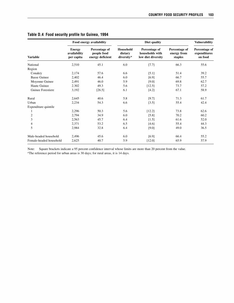
COUNTRY FOOD SECURITY PROFILES 103
Table D.4 Food security profile for Guinea, 1994
Food energy availability Diet quality Vulnerability
Energy Percentage of Household Percentage of Percentage of Percentage ofavailability people food dietary households with energy from expenditures
Variable per capita energy deficient diversitya low diet diversity staples on food
National 2,510 45.1 6.0 [7.7] 66.3 55.6Region
Conakry 2,174 57.6 6.6 [5.1] 51.4 39.2Basse Guinee 2,402 46.4 6.0 [6.9] 66.7 55.7Moyenne Guinee 2,491 46.0 5.9 [9.0] 69.8 62.7Haute Guinee 2.302 49.3 5.6 [12.5] 73.7 57.2Guinee Forestiere 3,192 [26.5] 6.1 [4.2] 67.1 58.9
Rural 2,645 40.6 5.8 [9.7] 71.3 61.7Urban 2,234 54.3 6.6 [3.5] 55.4 42.4Expenditure quintile
1 2,296 50.3 5.6 [12.2] 73.8 62.62 2,794 34.9 6.0 [5.8] 70.2 60.23 2,563 45.7 6.4 [1.5] 61.6 52.04 2,371 53.2 6.5 [4.6] 55.4 44.35 2,984 32.8 6.4 [9.0] 49.0 36.5
Male-headed household 2,496 45.6 6.0 [6.9] 66.4 55.2Female-headed household 2,625 40.7 5.9 [12.0] 65.9 57.9
Note: Square brackets indicate a 95 percent confidence interval whose limits are more than 20 percent from the value.aThe reference period for urban areas is 30 days; for rural areas, it is 14 days.
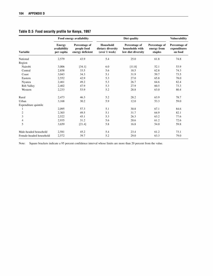
104 APPENDIX D
Table D.5 Food security profile for Kenya, 1997
Food energy availability Diet quality Vulnerability
Energy Percentage of Household Percentage of Percentage of Percentage ofavailability people food dietary diversity households with energy from expenditures
Variable per capita energy deficient (over 1 week) low diet diversity staples on food
National 2,579 43.9 5.4 25.0 61.8 74.8Region
Nairobi 3,006 [34.1] 6.0 [11.8] 52.1 53.9Central 2,858 33.5 5.6 18.5 62.8 74.3Coast 3,043 34.3 5.1 31.9 59.7 73.5Eastern 2,552 42.9 5.3 27.0 65.8 78.0Nyanza 2,461 49.2 5.3 26.7 64.6 82.4Rift Valley 2,402 47.9 5.3 27.9 60.5 73.3Western 2,233 53.9 5.2 28.8 63.0 80.4
Rural 2,473 46.3 5.2 28.2 63.9 78.7Urban 3,168 30.2 5.9 12.0 53.3 59.0Expenditure quintile
1 2,095 57.3 5.1 30.8 67.1 84.62 2,303 49.5 5.1 31.7 64.9 82.13 2,522 45.1 5.3 26.3 63.2 77.64 2,935 31.2 5.6 20.6 61.2 72.65 3,659 [21.4] 5.8 16.8 54.0 59.8
Male-headed household 2,581 45.2 5.4 23.4 61.2 73.1Female-headed household 2,572 39.7 5.2 29.0 63.3 79.0
Note: Square brackets indicate a 95 percent confidence interval whose limits are more than 20 percent from the value.
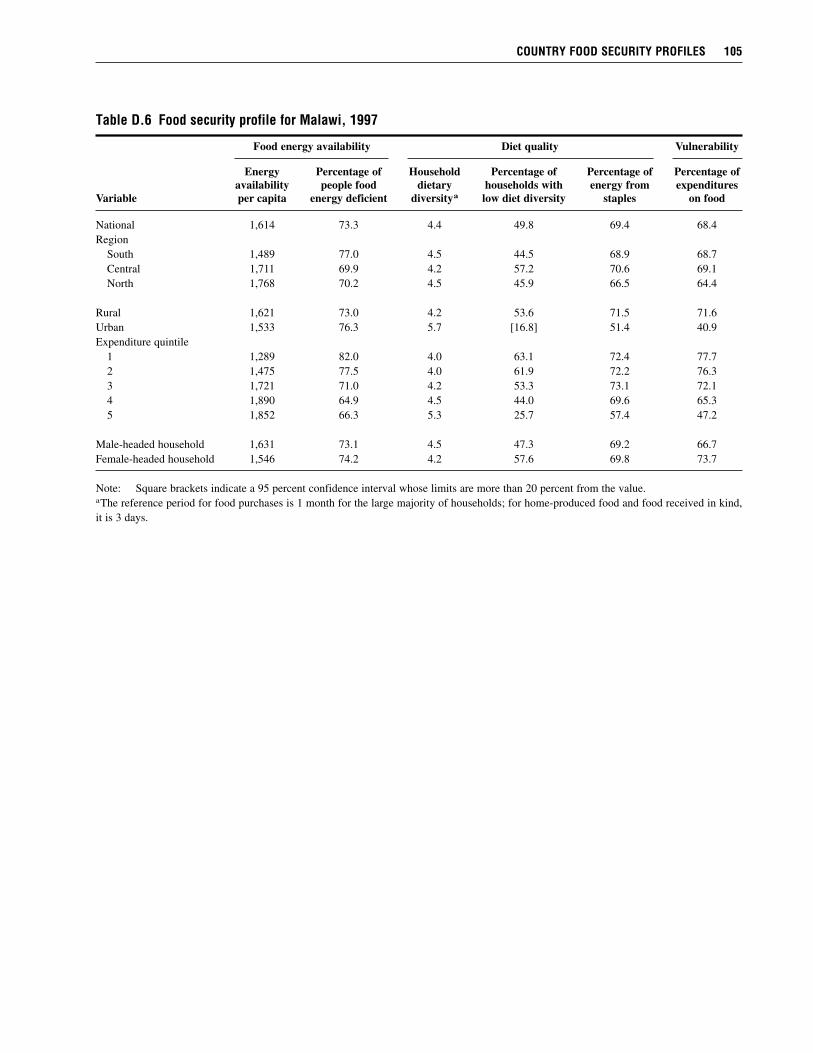
COUNTRY FOOD SECURITY PROFILES 105
Table D.6 Food security profile for Malawi, 1997
Food energy availability Diet quality Vulnerability
Energy Percentage of Household Percentage of Percentage of Percentage ofavailability people food dietary households with energy from expenditures
Variable per capita energy deficient diversitya low diet diversity staples on food
National 1,614 73.3 4.4 49.8 69.4 68.4Region
South 1,489 77.0 4.5 44.5 68.9 68.7Central 1,711 69.9 4.2 57.2 70.6 69.1North 1,768 70.2 4.5 45.9 66.5 64.4
Rural 1,621 73.0 4.2 53.6 71.5 71.6Urban 1,533 76.3 5.7 [16.8] 51.4 40.9Expenditure quintile
1 1,289 82.0 4.0 63.1 72.4 77.72 1,475 77.5 4.0 61.9 72.2 76.33 1,721 71.0 4.2 53.3 73.1 72.14 1,890 64.9 4.5 44.0 69.6 65.35 1,852 66.3 5.3 25.7 57.4 47.2
Male-headed household 1,631 73.1 4.5 47.3 69.2 66.7Female-headed household 1,546 74.2 4.2 57.6 69.8 73.7
Note: Square brackets indicate a 95 percent confidence interval whose limits are more than 20 percent from the value.aThe reference period for food purchases is 1 month for the large majority of households; for home-produced food and food received in kind,it is 3 days.
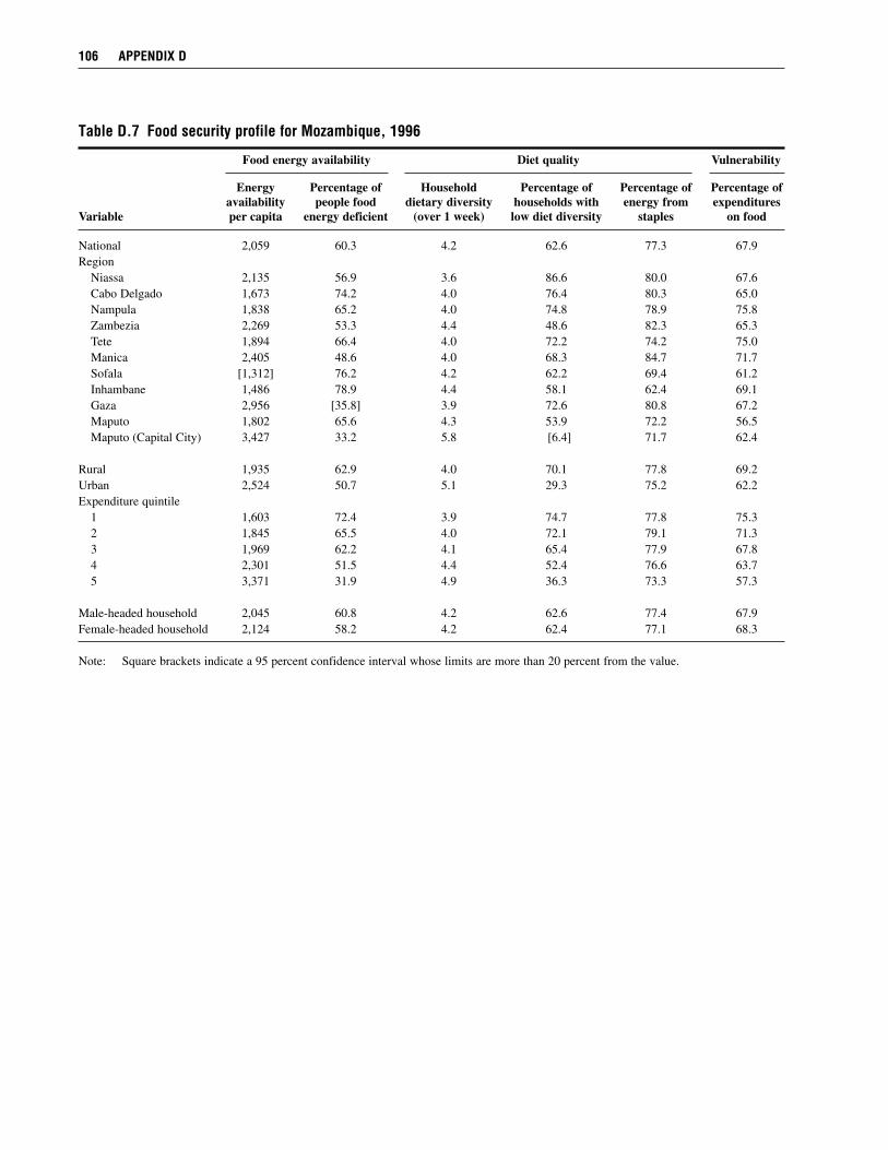
106 APPENDIX D
Table D.7 Food security profile for Mozambique, 1996
Food energy availability Diet quality Vulnerability
Energy Percentage of Household Percentage of Percentage of Percentage ofavailability people food dietary diversity households with energy from expenditures
Variable per capita energy deficient (over 1 week) low diet diversity staples on food
National 2,059 60.3 4.2 62.6 77.3 67.9Region
Niassa 2,135 56.9 3.6 86.6 80.0 67.6Cabo Delgado 1,673 74.2 4.0 76.4 80.3 65.0Nampula 1,838 65.2 4.0 74.8 78.9 75.8Zambezia 2,269 53.3 4.4 48.6 82.3 65.3Tete 1,894 66.4 4.0 72.2 74.2 75.0Manica 2,405 48.6 4.0 68.3 84.7 71.7Sofala [1,312] 76.2 4.2 62.2 69.4 61.2Inhambane 1,486 78.9 4.4 58.1 62.4 69.1Gaza 2,956 [35.8] 3.9 72.6 80.8 67.2Maputo 1,802 65.6 4.3 53.9 72.2 56.5Maputo (Capital City) 3,427 33.2 5.8 [6.4] 71.7 62.4
Rural 1,935 62.9 4.0 70.1 77.8 69.2Urban 2,524 50.7 5.1 29.3 75.2 62.2Expenditure quintile
1 1,603 72.4 3.9 74.7 77.8 75.32 1,845 65.5 4.0 72.1 79.1 71.33 1,969 62.2 4.1 65.4 77.9 67.84 2,301 51.5 4.4 52.4 76.6 63.75 3,371 31.9 4.9 36.3 73.3 57.3
Male-headed household 2,045 60.8 4.2 62.6 77.4 67.9Female-headed household 2,124 58.2 4.2 62.4 77.1 68.3
Note: Square brackets indicate a 95 percent confidence interval whose limits are more than 20 percent from the value.

COUNTRY FOOD SECURITY PROFILES 107
Table D.8 Food security profile for Rwanda, 2000
Food energy availability Diet quality Vulnerability
Energy Percentage of Household Percentage of Percentage of Percentage ofavailability people food dietary households with energy from expenditures
Variable per capita energy deficient diversitya low diet diversity staples on food
National 1,860 65.3 4.5 49.2 62.6 81.6Region
Butare 1,519 78.2 4.7 43.3 60.1 81.6Byumba 1,855 67.7 4.2 60.8 55.1 85.3Cyangugu 1,365 80.7 5.3 [21.2] 56.1 83.7Gikongor 1,721 70.9 3.9 65.5 69.7 85.9Gisenyi 1,742 68.6 4.5 46.9 66.5 82.9Gitarama 2,191 53.2 4.7 42.9 66.2 80.9Kibungo 2,334 48.5 4.7 45.4 65.3 80.8Kibuye 1,583 76.0 4.1 64.3 63.9 89.3Kigali Ngali 2,076 57.6 4.2 60.3 63.9 83.3Ville de Kigali 2,173 56.2 6.4 [3.3] 52.6 57.2Ruhengeri 1,669 70.3 3.9 67.6 65.8 84.7Umutara 1,917 63.3 4.2 61.9 64.1 81.3
Rural 1,824 66.5 4.3 54.1 63.6 84.2Urban 2,159 55.4 6.3 [4.9] 53.4 58.6Expenditure quintile
1 1,378 80.8 4.0 65.3 66.1 87.82 1,612 73.4 4.2 59.4 64.0 86.73 1,944 61.9 4.5 48.2 63.5 83.74 2,161 55.9 4.7 43.8 61.6 79.45 2,634 41.1 5.7 18.6 55.1 64.8
Male-headed household 1,903 64.1 4.7 45.2 62.0 81.0Female-headed household 1,746 68.6 4.3 57.9 63.8 83.1
Note: Square brackets indicate a 95 percent confidence interval whose limits are more than 20 percent from the value.aThe reference period for urban areas is 30 days, and the one for rural areas is 14 days.
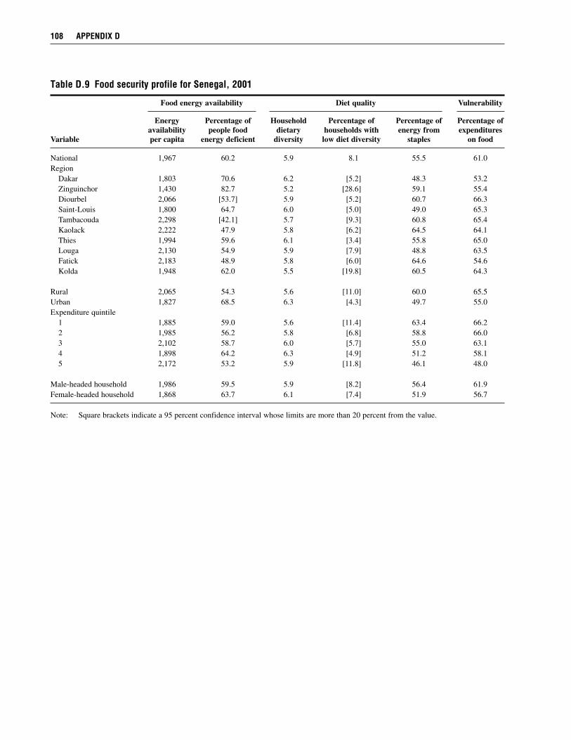
108 APPENDIX D
Table D.9 Food security profile for Senegal, 2001
Food energy availability Diet quality Vulnerability
Energy Percentage of Household Percentage of Percentage of Percentage ofavailability people food dietary households with energy from expenditures
Variable per capita energy deficient diversity low diet diversity staples on food
National 1,967 60.2 5.9 8.1 55.5 61.0Region
Dakar 1,803 70.6 6.2 [5.2] 48.3 53.2Zinguinchor 1,430 82.7 5.2 [28.6] 59.1 55.4Diourbel 2,066 [53.7] 5.9 [5.2] 60.7 66.3Saint-Louis 1,800 64.7 6.0 [5.0] 49.0 65.3Tambacouda 2,298 [42.1] 5.7 [9.3] 60.8 65.4Kaolack 2,222 47.9 5.8 [6.2] 64.5 64.1Thies 1,994 59.6 6.1 [3.4] 55.8 65.0Louga 2,130 54.9 5.9 [7.9] 48.8 63.5Fatick 2,183 48.9 5.8 [6.0] 64.6 54.6Kolda 1,948 62.0 5.5 [19.8] 60.5 64.3
Rural 2,065 54.3 5.6 [11.0] 60.0 65.5Urban 1,827 68.5 6.3 [4.3] 49.7 55.0Expenditure quintile
1 1,885 59.0 5.6 [11.4] 63.4 66.22 1,985 56.2 5.8 [6.8] 58.8 66.03 2,102 58.7 6.0 [5.7] 55.0 63.14 1,898 64.2 6.3 [4.9] 51.2 58.15 2,172 53.2 5.9 [11.8] 46.1 48.0
Male-headed household 1,986 59.5 5.9 [8.2] 56.4 61.9Female-headed household 1,868 63.7 6.1 [7.4] 51.9 56.7
Note: Square brackets indicate a 95 percent confidence interval whose limits are more than 20 percent from the value.

COUNTRY FOOD SECURITY PROFILES 109
Table D.10 Food security profile for Tanzania, 2000
Food energy availability Diet quality Vulnerability
Energy Percentage of Household Percentage of Percentage of Percentage ofavailability people food dietary diversity households with energy from expenditures
Variable per capita energy deficient (over 1 month) low diet diversity staples on food
National 2,454 43.9 5.9 9.7 70.6 72.5Region
Dodoma 2,764 [29.6] 6.0 [5.2] 74.5 73.2Arusha 2,307 [52.3] 6.0 [13.3] 68.6 73.9Kilimanjaro 2,043 61.0 6.3 [3.4] 61.1 79.3Tanga 2,379 [46.6] 5.9 [13.1] 72.5 73.9Morogoro 2,463 [42.1] 6.0 [5.1] 72.1 75.6Pwani 2,339 52.5 5.8 [4.9] 68.6 73.7Dar es Salaam 2,079 61.0 6.1 [8.1] 57.9 60.8Lindi [2,558] [51.5] 5.3 [20.5] 70.4 78.3Mtwara 2,648 [44.0] 5.5 [15.4] 68.1 73.3Ruvuma 2,557 [42.2] 5.3 [18.7] 76.5 68.6Iringa 2,575 [43.8] 5.8 [10.0] 71.4 78.2Mbeya 2,659 [27.1] 6.3 [4.4] 69.5 71.5Singida 2,249 [49.1] 5.6 [18.1] 73.9 77.2Tabora 2,936 [22.3] 6.2 [2.6] 73.2 74.0Rukwa 2,283 [53.9] 5.9 [5.1] 72.6 69.2Kigoma 2,482 47.8 5.9 [2.0] 72.1 70.8Shinyanga 2,776 [30.2] 5.9 [8.0] 77.3 71.7Kagera 2,289 [45.7] 5.9 [12.9] 65.2 73.0Mwanza 2,311 47.2 5.7 [11.1] 76.3 68.6Mara [2,215] [57.1] 5.6 [20.3] 73.2 72.0
Rural 2,487 41.8 5.8 [11.0] 72.8 74.4Urban 2,314 52.7 6.2 [5.1] 62.5 65.5Expenditure quintile
1 2,246 49.3 5.7 [13.1] 76.4 75.72 2,562 39.5 5.9 [10.1] 71.9 74.53 2,613 39.4 6.1 [5.5] 68.6 71.64 2,543 43.2 6.1 [5.5] 64.1 67.65 3,015 35.9 6.0 [9.5] 59.3 64.4
Male-headed household 2,460 44.2 5.9 [9.6] 70.7 72.7Female-headed household 2,427 42.8 5.9 [10.1] 69.9 71.8
Notes: Square brackets indicate a 95 percent confidence interval whose limits are more than 20 percent from the value. The highest differ-ence between the confidence interval limits and the value is 35 percent for the percentage of people food energy deficient in the regionof Lindi.

110 APPENDIX D
Table D.11 Food security profile for Uganda, 1999
Food energy availability Diet quality Vulnerability
Energy Percentage of Household Percentage of Percentage of Percentage ofavailability people food dietary diversity households with energy from expenditures
Variable per capita energy deficient (over 1 weeks) low diet diversity staples on food
National 2,636 36.8 4.4 50.9 69.4 59.3Region
Central 2,632 36.9 4.7 41.9 66.7 54.6Eastern 2,602 32.3 4.6 42.3 72.1 61.5Northern 2,087 58.1 4.1 61.0 64.7 63.0Western 3,089 25.5 4.0 64.5 73.6 60.1
Rural 2,658 36.3 4.2 56.5 71.6 61.3Urban 2,493 40.7 5.3 21.1 57.4 48.7Expenditure quintile
1 2,187 49.8 4.1 61.9 71.3 65.52 2,681 31.8 4.1 58.7 73.2 62.83 2,771 32.1 4.3 53.9 72.4 59.24 3,012 29.9 4.6 44.2 69.1 55.95 2,941 31.6 5.0 30.2 59.3 50.1
Male-headed household 2,687 34.7 4.5 48.6 69.1 59.5Female-headed household 2,460 44.4 4.2 57.2 70.1 58.9

COUNTRY FOOD SECURITY PROFILES 111
Table D.12 Food security profile for Zambia, 1996
Food energy availability Diet quality Vulnerability
Energy Percentage of Household Percentage of Percentage of Percentage ofavailability people food dietary households with energy from expenditures
Variable per capita energy deficient diversitya low diet diversity staples on food
National 1,764 71.1 4.6 43.7 78.0 66.2Region
Central 2,014 60.9 4.6 43.2 80.9 62.9Copperbelt 1,832 70.9 5.4 16.7 72.9 63.8Eastern 1,644 75.5 4.4 52.7 83.6 71.5Luapula 1,604 76.3 4.1 63.1 86.2 65.2Lusaka 1,823 70.5 5.6 13.2 71.2 56.9Northern 1,394 79.7 4.2 57.0 72.4 71.7Northwestern 2,067 60.6 4.0 64.4 82.4 73.6Southern 1,774 70.9 4.4 48.3 79.1 62.0Western 1,869 68.0 3.2 80.8 85.2 76.2
Rural 1,750 71.2 4.1 60.9 82.0 70.3Urban 1,788 70.9 5.6 11.8 70.7 58.7Expenditure quintile
1 1,475 79.9 4.0 64.0 83.4 72.42 1,722 71.6 4.2 54.7 81.8 68.93 1,847 67.9 4.7 40.5 77.4 65.44 1,958 66.8 5.2 24.1 72.8 61.05 2,445 50.7 5.7 14.4 67.4 57.8
Male-headed household 1,762 71.5 4.7 40.8 77.4 65.8Female-headed household 1,774 69.2 4.3 53.1 80.0 67.6
aThe reference period for purchases of maize is 30 days; for other purchased foods and foods from other sources, it is 14 days.

A P P E N D I X E
Methods of Estimating Global and RegionalFood Energy Deficiency Prevalences whenData Are Not Available for All Countries
Let countries be indexed by i = 1, . . . , N. The countries for which household survey dataexist are denoted C1, . . . , Cm. Those for which household survey data do not exist aredenoted Cm + 1, . . . , CN.
Method 1: Extrapolations Based on Cross-Country RegressionThis method draws on the extrapolation technique employed to estimate national poverty ratesby the World Bank’s Global Poverty Monitoring Facility. The estimation relies on individualcountry-specific characteristics for estimating energy deficiency rates of countries for whichsurvey data do not exist.
The extrapolations are undertaken using cross-country Ordinary Least Squares regressionsin which the regressors are variables describing various economic, social, political, and demo-graphic factors related to food insecurity. Candidates for these factors may be:• arable and irrigated land areas• foreign exchange earnings• per capita dietary energy supplies• per capita national incomes• income distribution• life expectancy• mortality rates• school enrollment rates• labor force participation rates• urbanization rates• conflict prevalences• degree of democracy• infrastructure index• population size• age distribution of the population
Where the goal is to estimate a developing-world prevalence, the region of location wouldalso be included as a regressor.
The following is the estimating equation for the extrapolations:
112

Uilog(—–—) =ΣK
k=1βk Xik + ui i = 1, . . . , m.
1 – Ui
The Xk are regressors, the βk are parametersto be estimated, and u is a stochastic errorterm. The logit transformation is used to re-strict the predicted values to lie within thetheoretical bounds (0,1) and to assure thatthe error term is unbounded (Ravallion, Datt,and van de Walle 1991).
Method 2: ExtrapolationsBased on Country-SpecificNonparametric DensityFunctions and Cross-Country RegressionThis method60 relies on the estimation ofempirical household energy availabilityprobability density functions, fi(x), for thecountries for which survey data exist topredict density functions for the remainingN – (m + 1) countries. The method is non-parametric. Rather than requiring an a priorispecification of a particular function form,the nonparametric approach is fully flexi-ble. It allows the data to select the most ap-propriate representation of the distribution(Goodwin and Ker 1998; DiNardo and To-bias 2001). The estimation takes place in twostages.
In the first stage, the populations ofcountries C1 through Cm are divided intoD groups, indexed d = 1, . . . , D, based onequal-sized energy availability intervals.Following, γdi, the proportion of the coun-tries’ populations falling into each group,are estimated from the survey data. D cross-country regressions are then undertaken(corresponding to the D energy availabilitygroups) in which the dependent variableis γdi and the predicting variables used in
Method 1 are the candidate regressors. Theresulting estimating equations are then usedto predict γdi , i = m + 1, . . . , N.
The set of D estimating equations is asfollows:
γ1ilog(———) = ΣK
k=1β1k Xki + u1i i = 1, . . . , m.
1 – γ1i
γ2ilog(———) = ΣK
k=1β2k Xki + u2i i = 1, . . . , m.
1 – γ2i
γDilog(———) = ΣK
k=1βDk Xki + uDi i = 1, . . . , m.
1 – γDi
In the second stage, a nonparametricdensity estimation technique is employed totrace out fi(x) for the N – (m + 1) countriesfor which survey data do not exist usingtheir predicted γdi . The specific techniqueemployed is the kernel method of smooth-ing to build continuous density functions.Here each country’s observations are sur-rounded by a symmetric weighting functionK satisfying the condition,61
∫∞
–∞K(t)dt = 1.
Let xd represent the mean energy avail-ability level of interval d. The kernel esti-mator of the probability density function ofx is given by
1 x – xd—– ΣD
d=1K (—–—–)Dh h
where h is a bandwidth parameter that con-trols the amount of smoothing. The propor-tion of each country’s population acquiringless than z calories can then be estimatednumerically.
ESTIMATING GLOBAL AND REGIONAL FOOD ENERGY DEFICIENCY PREVALENCES 113
60This method is founded on a discussion with Martin Ravallion of the World Bank.
61The weighting function K(t) is normally a symmetric probability density function (Goodwin and Ker 1998).

A P P E N D I X F
Differences in Food Security Measuresacross Total Expenditure Quintiles when Quintiles Are Not Based on Predicted Expenditures
114
Table F.1 Differences in food security measures across total expenditure quintiles when quintiles are not basedon predicted expenditures
Food energy availability Diet quality
Expenditure Energy availability Percentage people Household diet Percentage of householdsquintile per capita food energy deficient quality with low quality diet
Burundi (1998)Quintile 1 688 99.4 3.7 56.9
2 1,396 89.1 4.4 37.13 2,153 53.7 4.8 28.44 3,100 21.4 5.1 18.35 4,055 9.0 6.1 8.4
Ethiopia (1999)Quintile 1 1,190 97.7 4.3 50.8
2 1,637 80.3 4.8 32.63 1,930 60.0 5.0 22.74 2,119 50.4 5.3 14.85 2,146 57.8 5.7 5.4
Ghana (1998)Quintile 1 1,435 81.5 5.3 12.4
2 2,023 59.8 5.7 6.33 2,480 42.3 5.9 7.14 3,011 28.4 6.1 4.85 3,607 18.3 6.1 12.7
Guinea (1994)Quintile 1 1,769 67.3 5.4 16.5
2 2,767 31.8 6.1 4.63 3,095 31.5 6.3 4.34 2,927 36.0 6.6 3.75 3,309 24.9 6.5 13.4

DIFFERENCES IN FOOD SECURITY MEASURES ACROSS TOTAL EXPENDITURE QUINTILES 115
Table F.1—Continued
Food energy availability Diet quality
Expenditure Energy availability Percentage people Household diet Percentage of householdsquintile per capita food energy deficient quality with low quality diet
Kenya (1997)Quintile 1 1,365 86.6 4.3 44.4
2 2,076 52.4 5.1 25.33 2,686 28.1 5.5 21.54 3,389 16.2 5.8 16.85 4,470 10.0 6.0 16.3
Malawi (1997)Quintile 1 1,109 95.4 3.9 80.8
2 1,521 81.6 4.1 73.03 1,864 67.4 4.3 69.04 2,114 61.5 4.5 61.35 2,052 65.5 5.3 34.5
Mozambique (1996)Quintile 1 980 93.8 3.7 92.7
2 1,720 70.2 4.0 91.53 2,270 47.7 4.2 83.54 2,879 31.5 4.4 73.45 4,004 16.7 5.1 47.8
Rwanda (2000)Quintile 1 852 97.9 3.6 70.8
2 1,457 84.9 4.2 51.03 1,965 60.8 4.5 38.94 2,555 36.1 4.9 28.75 3,107 25.4 5.8 15.7
Senegal (2001)Quintile 1 1,437 78.8 5.5 10.4
2 1,908 60.0 5.8 6.03 2,113 55.7 6.1 5.54 2,322 49.4 6.2 3.75 2,660 36.8 6.1 10.5
Tanzania (2000)Quintile 1 1,723 68.8 5.5 31.3
2 2,501 35.5 5.9 18.43 2,928 26.7 6.1 12.54 3,280 20.1 6.2 10.15 4,072 11.6 6.2 8.5
Uganda (1999)Quintile 1 1,732 67.4 3.7 73.9
2 2,497 35.4 4.1 58.03 2,892 23.3 4.5 46.84 3,307 21.1 4.7 42.05 3,505 16.3 5.3 26.3
Zambia (1996)Quintile 1 1,151 89.8 3.6 69.7
2 1,697 73.7 4.3 47.83 1,881 67.7 4.8 33.24 2,228 57.8 5.3 22.45 2,802 36.9 5.7 16.1
Note: All values are corrected for survey sampling designs.

116
References
ACC/SCN (Administrative Committee on Coordination/Subcommittee on Nutrition of the United Na-tions). 2000. Fourth report on the world nutrition situation: Nutrition throughout the life cycle.Geneva: United Nations.
———. 2004. Fifth report on the world nutrition situation: Nutrition for improved development out-comes. Geneva: United Nations.
Aduayom, D., and L. C. Smith. 2003. Estimating undernourishment with household expenditure sur-veys: A comparison of methods using data from three Sub-Saharan African countries. In Mea-surement and assessment of food deprivation and undernutrition, 241–244. Rome: FAO.
Agren, G., and R. Gibson. 1968. Food composition table for use in Ethiopia I. Stockholm: Swedish In-ternational Development Authority, Addis Ababa: Ethiopian Nutrition Institute.
Alderman, H., M. Babita, G. Demombynes, N. Makhatha, and B. Ozler. 2002. How low can you go?Combining census and survey data for mapping poverty in South Africa. Journal of AfricanEconomies 11 (2): 169–200.
Arbia, G. 2003. The effect of sampling design on the reliability of estimates of the variance of distribu-tions derived from household survey data: A simulation study. In Measurement and assessmentof food deprivation and undernutrition, 249–250. Rome: FAO.
Arimond, M., and M. T. Ruel. 2004. Dietary diversity, dietary quality, and child nutritional status: Ev-idence from eleven demographic and health surveys. Report submitted to the Food and Nutri-tion Technical Assistance Project, Academy for Educational Development. Washington, D.C.:International Food Policy Research Institute.
Arndt, C., H. T. Jensen, and F. Tarp. 2000. Stabilization and structural adjustment in Mozambique: Anappraisal. Journal of International Development 12 (3): 299–323.
Becker, W. 2001. Comparability of household and individual food consumption data—evidence fromSweden. Public Health Nutrition 4: 1173–1176.
Behrman, J. R., and J. C. Knowles. 1997. How strongly is schooling associated with household income?PIER Working Paper No. 97-022. Penn Institute for Economic Research. Philadelphia: Univer-sity of Pennsylvania.
Blades, D. W. 1980. What do we know about levels and growth of output in developing countries?A critical analysis with special reference to Africa. In Economic growth and resources, vol. 2:Trends and flows, ed. R. C. Matthews, 60–77. London: Macmillan.
Bouis, H. 1994. The effect of income on demand for food in poor countries: are our food consumptiondatabases giving us reliable estimates? Journal of Development Economics 44: 19–226.
Bouis, H., and L. Haddad. 1992. Are estimates of calorie-income elasticities too high? A recalibrationof the plausible range. Journal of Development Economics 39: 333–364.
Bouis, H., L. Haddad, and E. Kennedy. 1992. Does it matter how we survey demand for food? Evidencefrom Kenya and the Philippines. Food Policy 17 (5): 349–360.
Bouis, H., B. de la Briere, L. Buitierrez, K. Hallman, N. Hassan, O. Hels, W. Quabili, A. Quisumbing,S. Thilsted, Z. Hassan Zihad, and S. Zohir. 1998. Commercial vegetable and polyculture fish

production in Bangladesh: their impacts on income, household resource allocation, and nutrition.Washington, D.C.: International Food Policy Research Institute.
Broca, S. 2003. Discussion group report—FAO method. In Measurement and assessment of food dep-rivation and undernutrition, 53–55. Rome: FAO.
Caldwell, R., M. Seroussi, C. Hagens, J. Huddle, C. Mbizule, and K. Uny. 2003. Malawi baseline sur-vey: Report of findings. Prepared for C-SAFE. Tucson, Ariz., U.S.A.: TANGO International.http://www.c-safe.org/downloads/Mal-baseline%20Fin-Report.doc.
China (People’s Republic of). 1992. Food consumption data from the urban and rural household surveysin China, 1985 and 1990. Prepared by the State Statistical Bureau, People’s Republic of China,in collaboration with the Statistical Analysis Service, Statistics Division, Economic and SocialPolicy Department, FAO. Rome: FAO.
David, I. P. 2003. Discussion opener—FAO method. In Measurement and assessment of food depriva-tion and undernutrition, 43–47. Rome: FAO.
Deaton, A. 1997. The analysis of household surveys: A microeconometric approach to developmentpolicy. Baltimore, Md., U.S.A.: Johns Hopkins University Press for the World Bank.
———. 2003. How to monitor poverty for the millennium development goals. Journal of HumanResources 4 (3): 353–378.
Deaton, A., and M. Grosh. 2000. Consumption. In Designing household survey questionnaires for de-veloping countries: Lessons from 15 years of the Living Standards Measurement Surveys,ed. M. Grosh and P. Glewwe, 91–133. Washington, D.C.: World Bank.
DiNardo, J., and J. L. Tobias. 2001. Nonparametric density and regression estimation. Journal of Eco-nomic Perspectives 15 (4): 11–28.
Dowler, E., and Y. Ok Seo. 1985. Assessment of energy intake: Estimates of food supply vs. measure-ment of food consumption. Food Policy 10 (August): 278–288.
ENI (Ethiopian Nutrition Institute). 1968. Expanded food composition table for use in Ethiopia. AddisAbaba.
Eyeson, K. K., and E. K. Ankrah. 1975. Composition of foods commonly used in Ghana. Food ResearchInstitute (CSIR) and United Nations Development Programme (UNDP) and the Food and Agri-culture Organization of the United Nations (FAO). Accra, Ghana: Food Research Institute.
FAO (Food and Agriculture Organization of the United Nations). 1983. A comparative study of foodconsumption data from food balance sheets and household surveys. Statistics Division, Eco-nomic and Social Development Paper 34. Rome: FAO.
———. 1996. Sixth world food survey. Rome: FAO.
———. 1999. Special report: FAO/WFP Crop and Food Supply Assessment Mission to Tanzania.Rome: FAO.
———. 2001. The state of food insecurity in the world 2001. Rome: FAO.
———. 2003. FAOSTAT database. http://apps.fao.org.
———. 2004a. Improvements in the estimation of the prevalence of undernourishment. Powerpointpresentation given at the Workshop on Measurement of Food Deprivation, October 22, Rome.http://www.fao.org/es/ESS/meetings/mofd_2004.asp.
———. 2004b. Women and food security. Rome: FAO. http://www.fao.org/FOCUS/E/Women/Sustin-e.htm.
———. 2005a. FAOSTAT. Food security statistics: Food needs. http://ww.fao.org/faostat/foodsecurity/Files/MinimumDietaryEnergyRequirement.xls.
———. 2005b. FAOSTAT. Food security statistics: Access to food. http://ww.fao.org/faostat/foodsecurity/Files/AccessToFoodGini.xls.
REFERENCES 117
FAO/WHO/UNU (Food and Agriculture Organization of the United Nations/World Health Organization/United Nations University). 1985. Protein and energy requirements. Rome: FAO.
Ferro-Luzzi, A. 2003. Individual food intake survey methods. In Measurement and assessment of fooddeprivation and undernutrition, 101–126. Rome: FAO.
FEWS NET. 1997. The uneven Ugandan recovery. December 27, 1997. USAID Famine Early WarningSystems Network. http://www.fews.net.
Filmer, D., and L. Pritchett. 1998. Estimating wealth effects without expenditure data—or tears: with anapplication to educational enrollments in states of India. World Bank Policy Research WorkingPaper No. 1994. Washington, D.C.: World Bank.
Frankenberger, T. R., L. Frankel, S. Ross, M. Burke, C. Cardenas, D. Clark, A. Goddard, K. Henry,M. Middleberg, D. O’Brien, C. Perez, R. Robinson, and J. Zielinski. 1997. Household liveli-hood security: A unifying conceptual framework for CARE programs. In Proceedings of theUSAID workshop on performance measurement for food security, Arlington, Va., U.S.A., De-cember 11–12, 1995. Washington, D.C.: U.S. Agency for International Development.
Frankenberger, T., K. Luther, K. Fox, and J. Mazzeo. 2003. Livelihood erosion through time: Macro andmicro factors that influenced livelihood trends in Malawi over the last 30 years. For CARESouthern and Western Africa Regional Management Unit (SWARMU). Tucson, Ariz., U.S.A.:TANGO International.
Friel, S., M. Nelson, K. McCormack, C. Kelleher, and P. L. Thriskos. 2001. Methodological issues usinghousehold budget survey expenditure data for individual food availability estimation: Irish ex-perience in the DAFNE pan-European project. Public Health Nutrition 4 (5B): 1143–1148.
FSANZ (Food Standards Australia New Zealand). 2004. Explanatory notes for use with the on-line nu-trition panel calculator (NPC). Supported by AUSNUT Special Edition (3) (Australian Food andNutrient Database for Nutrition Labelling, Release 3). Commonwealth of Australia and FoodStandards Australia New Zealand. http://www.foodstandards.gov.au/_srcfiles/Explanatory_notes_for_the_NPC_coldfusion_October_2004_final.pdf.
Gabbert, S., and H. P. Weikard. 2001. How widespread is undernourishment? A critique of measurementmethods and new empirical results. Food Policy 26 (3): 209–228.
Garrett, J. 1998. Food and nutrition security in Mozambique: Characteristics, determinants, and strategicinsights. In Understanding poverty and well-being in Mozambique: the first national assessment(1996–97). Chapter 4, pp. 203–267. Washington, D.C.: MPF/UEM/IFPRI.
Gillen, E. D. 2004. Food consumption estimates; data sources, problems, and limitations; improve-ments. Powerpoint presentation given at the Workshop on Measurement of Food Deprivation,October 22, 2004. Rome: FAO. http://www.fao.org/es/ESS/meetings/mofd_2004.asp.
Gladwin, C., and A. Thomson. 2004. Food or cash crops? Which is the key to food security? Preparedfor the University of Florida’s Gender and Soil Fertility in Africa web page (http://www.fred.ifas.ufl.edu/CRSP/food.htm). Gainesville, Fla., U.S.A.: University of Florida.
Goodwin, B. K., and A. P. Ker. 1998. Nonparametric estimation of crop yield distributions: Implicationsfor rating group-risk crop insurance contracts. American Journal of Agricultural Economics 80(1): 139–153.
Government of Tanzania. 2000. Rapid assessment report on crop and food supply situation in Tanzaniafor the 1999/2000 agricultural season. Coordinated by the Disaster Management Department ofthe Office of the Prime Minister and the Food Security Department of the Ministry of Agricul-ture and Cooperatives, Dar es Salaam. July 25, 2000.
Graham, R., R. M. Welch, and H. E. Bouis. 2004. Addressing micronutrient malnutrition through en-hancing the nutritional quality of staple foods: Principles, perspectives and knowledge gaps.Department of Plant Science, University of Adelaide; U.S. Plant, Soil and Nutrition Laboratory,USDA-ARS, Ithaca, N.Y.; International Food Policy Research Institute, Washington, D.C.http://www.css.cornell.edu/FoodSystems/AdvAgron4.html.
118 REFERENCES

Green, W. H. 1997. Econometric Analysis. 3d ed. Upper Saddle River, N.J., U.S.A.: Prentice Hall.
Haddad, L. 2001. DfID-funded technical support facility to FAO’s FIVIMS. Technical Paper 1. Deepen-ing the analysis of the factors behind progress towards WFS targets. Report submitted to Over-seas Development Institute. Washington, D.C.: International Food Policy Research Institute.
Haddad, L., and R. Kanbur. 1990. How serious is the neglect of intrahousehold inequality? EconomicJournal 100 (402): 866–881.
Haddad, L., J. Hoddinott, and H. Alderman, eds. 1997. Intrahousehold resource allocation in develop-ing countries: Models, methods, and policy. Baltimore, Md., U.S.A., and London: Johns Hop-kins University Press for the International Food Policy Research Institute.
Higgins, P. A., and H. Alderman. 1997. Labor and women’s nutrition: The impact of work effort and fer-tility on nutritional status in Ghana. Journal of Human Resources 32 (3): 577–595.
Hoddinott, J., ed. 2001. Food security in practice: Methods for rural development projects. Washington,D.C.: International Food Policy Research Institute.
ICN (International Conference on Nutrition). 1992. Caring for the socioeconomically deprived and nu-tritionally vulnerable. Major Issues for Nutrition Strategies Theme Paper No 3. ICN/92/INF/7.Rome: FAO and World Health Organization.
IFPRI (International Food Policy Research Institute). 1998. 2020 Vision Network for West Africa: Coun-try Note for Senegal. Accra, Ghana: IFPRI.
Kennedy, E. 2003. Qualitative measures of food insecurity and hunger. In Measurement and assessmentof food deprivation and undernutrition, 165–180. Rome: FAO.
Lagiou, P., A. Trichopoulou, and the DAFNE contributors. 2001. The DAFNE initiative: The method-ology for assessing dietary patterns across Europe using household budget survey data. PublicHealth Nutrition 4: 1135–1142.
Landis, J. R., and G. G. Koch. 1977. The measurement of observer agreement for categorical data. Bio-metrics 33 (1): 159–174.
Latham, M. C. 1997. Human nutrition in the developing world. Food and Nutrition Series No. 29.Rome: FAO. http://www.fao.org/DOCREP/W0073e/w0073e00.htm.
Lence, S. 2003. Discussion opener—Household expenditure survey methods. In Measurement and as-sessment of food deprivation and undernutrition. Rome: FAO.
Leung, W.-T. W. 1968. Food composition table for use in Africa. Rome: FAO, and Bethesda, Md.,U.S.A.: U.S. Department of Health, Education, and Welfare.
Mason, J. 2003. Measuring hunger and malnutrition. In Measurement and assessment of food depriva-tion and undernutrition, 197–228. Rome: FAO.
Maxwell, S., and T. R. Frankenberger. 1992. Household food security: Concepts, indicators, measure-ments: A technical review. New York and Rome: United Nations Children’s Fund and Interna-tional Fund for Agricultural Development.
Maxwell, D. G., A. Clement, C. E. Levin, M. Armar-Klemesu, S. Zakariah, and G. M. Lamptey. 1999.Alternative food-security indicators: Revisiting the frequency and severity of “coping strate-gies.” Food Policy 24 (4): 411–429.
Mozambique. 1991. Tabela de Composição de Alimentos. Maputo, Mozambique: Ministry of Health,Nutrition Section.
Naiken, L. 2003. FAO methodology for estimating the prevalence of undernourishment. In Measure-ment and assessment of food deprivation and undernutrition, 7–42. Rome: FAO.
Naska, A., S. Paterakis, H. Eeckman, A. M. Remaut, and K. Trygg. 2001. Methodology for renderinghousehold budget and individual nutrition surveys comparable, at the level of the dietary infor-mation collected. Public Health Nutrition 4: 1153–1158.
REFERENCES 119

Naska, A., V. G. S. Vasdekis, and A. Trichopoulou. 2001. A preliminary assessment of the use of house-hold budget survey data for the prediction of individual food consumption. Public Health Nu-trition 4: 1159–1166.
NBST (National Bureau of Statistics of Tanzania). 2002. Household Budget Survey 2000/01. Dar esSalaam: NBST.
Ndaiye, A. M. 1993. Aliments Africains: Table de composition. Dakar, Senegal: Organisme deRecherches sur l’Alimentation et la Nutrition Africaines (ORANA).
Ndaiye, A. 2003. Child malnutrition in Niger: An investigation of patterns of change. M.A. thesis, De-partment of Agricultural and Resource Economics, University of Arizona, Tucson, Ariz., U.S.A.
Nordeide, M. B. 2003. The composition of Malian foods. Bamako, Mali: CNRST, Programme deRecherche SSE, and Oslo, Norway: Nordic School of Nutrition, University of Oslo.
Nyanteng, V. K., and S. Asuming-Brempong. 2003. The role of agriculture in food security in Ghana.Paper prepared for the Role of Agriculture International Conference, Rome, October 20–22.Rome: FAO.
Oguntona, E. B., and I. O. Akinyele, eds. 1995. Nutrient composition of commonly eaten foods in Nigeria—Raw, processed and prepared. Food Basket Foundation Publication Series. Ibadan, Nigeria: FoodBasket Foundation International.
Pellet, P. L., and S. Shadarevian. 1970. Tables for use in the Middle East, 2d ed. Beirut, Lebanon: Amer-ican University of Beirut.
Platt, B. S. 1962. Tables of representative values of foods commonly used in tropical countries. London:Medical Research Council. (Reprinted 1985 by the London School of Hygiene and TropicalMedicine, Department of Human Nutrition, by permission of the Controller of Her Majesty’sStationery Office.)
Quisumbing, A., L. Haddad, and C. Peña. 2001. Are women overrepresented among the poor? Ananalysis of poverty in ten developing countries. Journal of Development Economics 66 (1):225–269.
Ravallion, M. 2001. Measuring aggregate welfare in developing countries: How well do national ac-counts and surveys agree? Washington, D.C.: World Bank.
Ravallion, M., G. Datt, and D. van de Walle. 1991. Quantifying absolute poverty in the developingworld. Review of Income and Wealth 37 (4): 345–361.
Resnick, D. 2004. Smallholder African agriculture progress and problems in confronting hunger andpoverty. Development Strategy and Governance Division Discussion Paper 9. Washington,D.C.: International Food Policy and Research Institute.
Rimmer, D. J. 2001. An overview of food eaten outside the home in the United Kingdom National FoodSurvey and the new Expenditure and Food Survey. Public Health Nutrition 4: 1173–1176.
Ruel, M. T. 2002. Is dietary diversity an indicator of food security or dietary quality? A review of mea-surement issues and research needs. Food Consumption and Nutrition Division DiscussionPaper 140. Washington, D.C.: International Food Policy Research Institute.
Ruel, M. T. 2003. Operationalizing diet diversity: A review of measurement issues and research priori-ties. Journal of Nutrition 133 (11): 3911S–3926S.
Ruel, M., and J. Garrett. 2004. Features of urban food and nutrition security and considerations for suc-cessful urban programming. Electronic Journal of Agricultural and Development Economics 1(2). http://www.fao.org/es/esa/en/ejade.htm.
Ruel, M. T., L. Haddad, M. Arimond, D. Gilligan, N. Minot, K. Simler, and X. Zhang. 2003. Diet qual-ity and diet changes of the poor: A global research program to improve dietary quality, health,and nutrition. A proposal for a global research program (GRP24). Washington, D.C.: Interna-tional Food Policy Research Institute.
120 REFERENCES
Ruel, M. T., J. M. Graham, S. Murphy, and L. H. Allen. 2004. Simple dietary diversity indicators pre-dict nutrient adequacy in school-age Kenyan children. Report submitted to GL-CRSP. Wash-ington, D.C.: IFPRI.
Sachs, J. 2004. Doing the sums on Africa. Economist May 20, 2004, 19–21.
Sehmi, J. K. 1993. National food composition tables and the planning of satisfactory diets in Kenya.Nairobi: Ministry of Health, Government of Kenya.
Senauer, B. 2003. FAO methodology for estimating the prevalence of undernourishment. Discussionopener. In Measurement and assessment of food deprivation and undernutrition, 49–52. Rome:FAO.
Senauer, B., and M. Sur. 2001. Ending global hunger in the 21st century: Projections of the number offood insecure people. Review of Agricultural Economics 25 (spring/summer): 68–81.
Shapouri, S., and S. Rosen. 1999. Food security assessment: Why countries are at risk. AgriculturalInformation Bulletin No. 754. Washington, D.C.: Economic Research Service, United StatesDepartment of Agriculture.
Shetty, P. 2003. Measures of nutritional status from anthropometric survey data. In Measurement andassessment of food deprivation and undernutrition, 139–154. Rome: FAO.
Smith, L. C. 1998a. Can FAO’s measure of chronic undernourishment be strengthened? Food Policy 23(4): 425–445.
———. 1998b. Can FAO’s measure of undernourishment be strengthened? With a response byL. Naiken. Food Consumption and Nutrition Division Discussion Paper 44. Washington, D.C.:International Food Policy Research Institute.
———. 2003. The use of household expenditure surveys for the assessment of food insecurity. InMeasurement and assessment of food deprivation and undernutrition, 57–88. Rome: FAO.
Smith, L., A. El Obeid, H. Jensen, and S. R. Johnson. 1999. The geography and causes of food insecu-rity in developing countries. Chapter 5 in Food security: New solutions for the 21st century, ed.A. El Obeid, S. R. Johnson, H. Jensen, and L. Smith. Ames, Iowa, U.S.A.: Iowa State Univer-sity Press.
Srivastava, A. K., A. Rai, and V. Ramasubramanian. 2003. On reliability of estimates of inequality indistributions derived from sample survey data. In Measurement and assessment of food depri-vation and undernutrition, 245–248. Rome: FAO.
StataCorp. 2003. Stata 8 Reference Manual. College Station, Tex., U.S.A.: Stata Corporation.
Statsoft. 2005. Nonparametric statistics. Electronic Statistics Textbook. Tulsa, Okla.: Statsoft. http://www.statsoftinc.com/textbook/stnonpar.html.
Svedberg, P. 1999. 841 million undernourished? World Development 27 (12): 2081–2098.
———. 2000. Poverty and undernutrition: Theory, measurement, and policy. Oxford: Oxford Univer-sity Press.
———. 2003. Fallacies in—and ways of improving—the FAO methodology for estimating prevalenceof undernutrition. In Measurement and assessment of food deprivation and undernutrition,235–236. Proceedings of an International Scientific Symposium. Rome: FAO.
Swindale, A., and P. Ohri-Vachaspati. 2004. Measuring household food consumption: A technical guide.Washington, D.C.: Food and Nutrition Technical Assistance (FANTA) Project and Academy forEducational Development (AED).
Tanzania. 2000. Rapid assessment report on crop and food supply situation in Tanzania for the 1999/2000 agricultural season. Coordinated by the Disaster Management Department of the Officeof the Prime Minister and the Food Security Department of the Ministry of Agriculture and Co-operatives, Dar es Salaam.
REFERENCES 121

Trochim, W. M. 2001. The research methods knowledge base, 2nd ed. http://trochim.human.cornell.edu/kb/index.htm (version current as of 2001).
UNDHA (United Nations Department of Humanitarian Affairs). 1996. Great Lakes: IRIN Food Secu-rity Overview Paper. 12/23/96. New York: Integrated Regional Information Network (IRIN),UNDHA.
UNICEF (United Nations Children’s Fund). 1998. The state of the world’s children 1998. New York:Oxford University Press.
USDA (United States Department of Agriculture). 1963. Composition of foods. Washington, D.C.:USDA.
———. 1998. Composition of foods commonly eaten. Data files. Washington, D.C.: USDA.
———. 1999. USDA nutrient database for standard reference, release 13. Washington, D.C.: USDA.
———. 2002. USDA nutrient database for standard reference, release 15. Washington, D.C.: USDA.
——— 2003. Composition of foods, raw, processed, prepared. USDA nutrient database for standardreference, release 15. Beltsville, Md., U.S.A.: USDA Agricultural Research Service.
U.S. Department of State. 2004. Background note Guinea. April. Washington, D.C.: Bureau of AfricanAffairs.
USDHEW/FAO (United States Department of Health, Education, and Welfare/Food and AgricultureOrganization of the United Nations). 1968. Food composition table for use in Africa. Bethesda,Md., U.S.A.: USDA, and Rome: FAO.
Vasdekis, B. G. S., S. Stylianou, and A. Naska. 2001. Estimation of age- and gender-specific food avail-ability from household budget survey data. Public Health Nutrition 4 (5B): 1149–1152.
Welch, R. 2004. Micronutrients, agriculture, and nutrition: Linkages for improved health and well being.USDA-ARS, U.S. Plant, Soil and Nutrition Laboratory, Ithaca, N.Y. http://www.css.cornell.edu/FoodSystems/Micros%26AgriMan1ref.html.
West, C. E., F. Pepping, I. Scholte, W. Jansen, and H. F. F. Albers. 1987. Food composition table for en-ergy and eight important nutrients in foods commonly eaten in East Africa (Poster). Wagenin-gen, The Netherlands: Technical Centre for Agriculture and Rural Cooperation (CTA) of ACP/ECP Convention of Lome, and Food and Nutrition Cooperation (ECSA), Department of HumanNutrition, Wageningen Agricultural University, and Dar es Salaam, Tanzania: Tanzania Foodand Nutrition Centre.
West, C. E., F. Pepping, and C. R. Temalilwa, eds. 1988. The composition of foods commonly eaten inEast Africa. Wageningen, The Netherlands: Wageningen Agricultural University.
WHO (World Health Organization). 2003. WHO Global database on child growth and malnutrition.Geneva: WHO.
Williamson, J. 1975. Useful plants of Malawi, rev. ed. Limbe: Montfrort.
Wobst, P. 2001. Structural adjustment and intersectoral shifts in Tanzania. Research Report 117. Wash-ington, D.C.: International Food Policy Research Institute.
World Bank. 2003. 2003 world development indicators. Washington, D.C.: World Bank.
———. 2004. Country brief, Burundi, history. http://web.worldbank.org/WBSITE/EXTERNAL/COUNTRIES/AFRICAEXT/ BURUNDIEXTN.
Zhang, X., M. Johnson, D. Resnick, and S. Robinson. 2004. Cross-country typologies and developmentstrategies to end hunger in Africa. Development Strategy and Governance Division DiscussionPaper 8. Washington, D.C.: International Food Policy Research Institute.
122 REFERENCES