1

OPEC’s Impact on Oil Price Volatility: The Role of Spare Capacity

Axel Pierru

King Abdullah Petroleum Studies and Research Center

James L. Smith*

Southern Methodist University

Tamim Zamrik

King Abdullah Petroleum Studies and Research Center

Abstract

OPEC claims to hold and use spare production capacity to stabilize the crude oil market. We

study the impact of that buffer on the volatility of oil prices. After estimating the stochastic

process that generates shocks to demand and supply, and OPEC’s limited ability to accurately

measure and offset those shocks, we find that OPEC’s use of spare capacity has reduced

volatility, perhaps by as much as half. We also apply the principle of revealed preference to

infer the loss function that rationalizes OPEC’s investment in spare capacity and compare it

to other estimates of the cost of supply outages.

* Corresponding author. Edwin L. Cox School of Business, Southern Methodist University,

Dallas, TX 75275. Email: jsmith@mail.cox.smu.edu, Phone: 214-768-3158.

Keywords: oil, price volatility, spare capacity, OPEC, revealed preference

JEL Codes: Q41, Q02, L11

2

1. Introduction

Spare production capacity plays a central role in the world oil market, and the spare

capacity held by OPEC members in particular is significant for its potential ability to stabilize

the market price. Indeed, to “ensure the stabilization of oil markets” is part of OPEC’s statutory

mission1. Often, the question has been raised whether OPEC’s spare capacity is large enough—

or too large (Fattouh, 2006; Petroleum Economist, 2008a,b; Saudi Gazette, 2013). Our purpose

in this paper is to shed light on the factors that have influenced OPEC’s calculation of the

volume of spare capacity required to achieve its mission, and to estimate the extent to which

OPEC’s utilization of spare capacity has stabilized the price of crude oil.

Looking beyond OPEC as a whole, we also focus on the spare capacity held by four

OPEC members: Saudi Arabia, Kuwait, Qatar, and the UAE. For lack of a better name, like

Reza (1984) and Alhajji and Huettner (2000) we will refer to these four as the OPEC Core

(Jacoby and Paddock (1983), Karp and Newberry (1991), and Gately (2004) use other

definitions for the Core). They are distinguished by a perception that, unlike many other

members, they have engaged most purposefully in attempts to balance the market by adjusting

their production to offset demand and supply shocks. Although the four Core members do not

necessarily act in unison to develop and manage spare capacity as a homogeneous unit, they

appear individually at least to have taken seriously the responsibility to help stabilize price. In

any event, the volume of spare capacity held by the Core comprises the largest portion of

OPEC’s total, averaging 85% during the period of our study.

The significance of efforts to stabilize the price of oil hardly requires explanation. The

market is exposed to substantial shocks that disrupt both supply and demand. Whether from

war, natural disasters, labor strikes, port closures, political sanctions, or terrorism, the

1 The complete mission statement is available at:

http://www.opec.org/opec_web/en/about_us/23.htm (accessed on July 28, 2015).

3

production and delivery of oil to the market is insecure and subject to frequent and

unpredictable outages. The demand for oil responds fitfully to the vagaries of the global

business cycle and financial markets, and suffers as well from other types of disruptions (e.g.,

the short-term substitution of diesel for nuclear energy after Fukushima, or diesel for coal prior

to the 2008 Summer Olympics). The impact of each disruption is further magnified by

relatively low elasticities of demand and supply, which means sharp price movements may be

required—especially in the short term—to restore equilibrium in the market.

Previous research (Jaffe and Soligo, 2002; Parry and Darmstadter, 2003; Kilian, 2008;

Baumeister and Gertsman, 2013; Brown and Huntington, 2015) has identified various

economic costs associated with oil price volatility. Some of these costs are borne directly by

the consumers and producers of crude oil and related products. They take the form of shocks

to factor prices and revenue streams that make long-term business planning more difficult but

also more important. Many private remedies exist to mitigate these shocks, including

precautionary inventories, hedging, and long-term contracts. Such measures impose costs of

their own, but for many it is the lesser of two evils. Rational consumers and producers are

guided by internal incentives that reflect their particular vulnerabilities, and these private

incentives are reflected in the extensive scope and diverse form of private risk management

programs that target the price of oil. Less direct is the impact of oil price shocks on the business

cycle and overall health of the economy. Viewing macroeconomic stability and national

security as a public good, national governments and various multilateral agencies have

attempted to manage these costs collectively, one example being the International Energy

Agency’s strategic petroleum reserve program that requires member nations to maintain 90

days of net oil import volumes in public storage. The European Union’s program, which is

more stringent, requires all members to maintain in public storage a volume equivalent to 90

days of domestic oil consumption.

4

In light of the various private and public incentives that motivate multiple entities to

manage oil price risks, it is clear that OPEC’s mission to stabilize the oil market is but one part

of a larger picture. OPEC’s role is unique, however, because it aspires to reduce price volatility

directly—by acting as a swing producer that offsets physical shocks to supply and demand—

rather than simply mitigating the cost of price shocks after they have occurred. This strategic

capability to reduce price volatility at its source is lacking in private commercial inventories

and government stockpiles. No privately-owned inventories are large enough to impact the

market price (and if several private entities collaborated in the effort, they could be charged

with illegal efforts at price fixing). Moreover, the public-good aspect of price stabilization

transcends the incentives of individual economic agents. Government stockpiles, although

certainly large enough (if released) to impact the price, are seldom used, perhaps because they

tend to be reserved for use during “emergencies” and because the rules for releasing volumes

to the market (or taking volumes off the market) are vague and controversial2.

Recent suggestions that privately-produced shale oil has taken OPEC’s place as the new

swing producer are misguided. The producers of shale oil do not regulate their output to offset

shocks to demand or supply, nor do individual shale oil producers have the ability or desire to

attempt to “defend” any particular price level. Even though it may represent something like an

expansion of privately owned and production-ready inventory, shale oil is produced subject to

the profit motive where the market price determines the quantity supplied, not vice versa. In

contrast, as we will show below, OPEC’s spare production capacity appears to be managed

2 Enabling legislation for the US Strategic Petroleum Reserve (Public Law 94-163-Dec. 22, 1975) states

its purpose as being to reduce “the impact of severe energy supply interruptions.” Recent press reports

indicate that the Obama administration has suggested the President be given the authority to release

barrels not only in reaction to likely economic harm caused by a supply disruption, but also in

anticipation of such developments. Those same reports indicate, however, that the administration is

very sensitive to suggestions that its focus on energy security amounts to managing markets (Petroleum

Intelligence Weekly, 2015). The International Energy Agency is very clear that the purpose of its

emergency stockholding program is not to manage oil prices. See

http://www.iea.org/topics/energysecurity/subtopics/energy_security_emergency_response/ (accessed

July 29, 2015).

5

actively (albeit not perfectly) to offset short-term fluctuations in demand and supply whether

or not that effort contributes to the profits of its members.

Before proceeding further, it is well to consider whether the purpose of OPEC’s spare

capacity is indeed to stabilize the market price. We find support for this proposition not only

in OPEC’s own mission statement, but also in the obvious and persistent efforts by some OPEC

members to raise or lower production to offset unexpected shocks to global demand and supply.

Many examples can be cited (e.g., production cuts during the global economic downturn in

2001, production increases which accompanied the unusual buildup of global demand in 2003-

2004 and supply disruptions in 2011-2012).

Such examples are typical of a “swing producer” and are indicative of the

organization’s commitment to stabilize the market. Khalid Al-Falih, then Saudi Aramco CEO,

acknowledged as much when reporting (Petroleum Economist, 2013) that “in the past two years

alone, we have swung our production by more than 1.5 million barrels a day (mmb/d) in order

to meet market supply imbalances.” Quite often Saudi Arabia is singled out as the ultimate

swing producer, the supplier of last resort with sufficient wherewithal (physical and financial)

to assume this duty3. Accordingly, in addition to studying the impact of OPEC and its four

Core members, we also perform a separate analysis of Saudi Arabia’s role in stabilizing the

market.

In principle, spare capacity could be used to advance objectives besides price

stabilization. One potential use would be to make opportunistic sales from spare capacity when

the market is tight—cherry picking to enhance sales revenue. We do not believe the evidence

supports this view. If demand for OPEC oil is inelastic, it is true that taking oil off the market

3 See, for example, Fattouh and Mahadeva’s (2013) review of the literature, in which Saudi Arabia is

singled out as the dominant swing producer. Nakov and Nuño (2013) show that both the size of Saudi

Arabia’s spare capacity and the volatility of its monthly output greatly exceed that of other OPEC

members.

6

when prices are low would increase revenue. But raising production when prices are high

would decrease revenue. In other words, opportunistic behavior must be asymmetric. In

reality, OPEC’s behavior appears to be more or less symmetric—not only raising output when

the market is tight but also cutting output when the market is weak. This pattern contradicts

the notion that spare capacity is held for the purpose of making opportunistic sales. If demand

is elastic, then taking oil off the market when prices are low would reduce sales revenue. Given

OPEC’s historic tendency to decrease production when facing surplus, this again contradicts

the hypothesis that OPEC’s spare capacity is managed opportunistically.

Another possibility is that OPEC employs its spare capacity to stabilize its own export

revenues. But then, assuming that demand is elastic, the prescribed course would be to decrease

production when an outage occurs. The logic here is simple: if a shock drives the market price

up (which ceteris paribus would increase OPEC revenue), then production must be decreased

to restore the previous (lower) level of revenue. This is not consistent with observed behavior.

Only if demand is inelastic would revenue stabilization and price stabilization dictate similar

actions. But then, even if the actual motive were to stabilize its own export revenues, by so

doing OPEC would also tend to stabilize the price.

After reviewing some related literature in Section 2, we develop in Section 3 a structural

model of a producer using his spare capacity to stabilize the market price of its output. We

estimate the model’s parameters using observed price and spare capacity data for three groups

of producers: Saudi Arabia, OPEC Core, and OPEC. In section 4, based on our model, we

derive an analytical formula for the marginal value of spare capacity. In Section 5, we adopt

the assumption that OPEC has equated the marginal costs and perceived benefits of its spare

capacity and invoke the principle of revealed preference to calibrate the loss function that

appears to have motivated OPEC’s investment in spare capacity. In section 6, our estimate of

OPEC’s loss function is compared to the estimated size of economic losses due to oil supply

7

disruptions derived from a well-known macroeconomic model of the global economy. The

extent to which each group of producers’ intervention has damped price volatility during the

past fifteen years is examined in Section 7, through both an analytical approach and a

counterfactual reconstruction of “unstabilized” price. Concluding observations are presented

in Section 8.

2. Related Literature

Here we discuss only the few papers that have previously addressed OPEC’s role in

stabilizing the price of oil and leave aside countless others that focus mainly on the level rather

than stability of price. De Santis (2003) attributed price volatility under OPEC’s old production

quota regime specifically to the inelasticity of Saudi Arabian supplies. Any physical

disruption, he argued, would create a short-term price spike that could only be dissipated by

longer term supply adjustments. De Santis assumed the absence of spare capacity which begs

the question of how such a precautionary buffer would be sized and managed—or what would

be its impact on price volatility.

Nakov and Nuño (2013) take the opposite approach, assuming that Saudi Arabia can

and does adjust its output in response to each monthly demand shock in the manner of a

Stackelberg dominant producer. By offsetting positive (negative) shocks with an increase

(decrease) in its own output, Saudi Arabia effectively reduces price volatility, although that

result is a by-product and not the objective of its behavior. The Stackelberg framework is a

very insightful approach that seems appropriate to the structure of the world oil market, but

one that presumes the dominant producer can perfectly anticipate the magnitude of each shock.

Substantial misjudgments in that regard, if acted upon, could in fact lead to an increase in

volatility, and the possibility of mistakes may hold the producer in abeyance.

Fattouh (2006) provided evidence that an increase in volatility and the frequency of

price spikes are in a general way due to reduced spare capacity held by OPEC and other

8

producers, but he did not pursue the argument to the point of a formal model or empirical

estimates. Kilian (2008) argues that large oil price increases were caused by the conjunction of

demand shifts and capacity constraints due to low OPEC and world spare capacity. Baumeister

and Peersman (2013) attribute the observed increase in volatility to substantial reductions in

short-run demand and supply elasticities post-1985. Difiglio (2014) recognizes OPEC’s role in

stabilizing prices via spare capacity and reviews reasons why similar efforts to offset

disruptions using consuming nations’ own strategic petroleum reserves have not been very

successful. However, he provides no model or structural framework by which the effectiveness

of releases from consumer stockpiles can be measured. More generally, the stockpile valuation

literature has applied a mixture of dynamic programming and more heuristic analysis to size

reserves designed to be used in disrupted periods only (see for instance Murphy and Oliveira

(2010) for a survey of the literature). The literature has not so far provided any formal model

of a buffer capacity that is used to continuously stabilize the price of oil, which is the goal of

our paper.

3. A Model of price stabilization using spare capacity

3.1 Model assumptions

Since there is nothing specific to OPEC in the structure of the model, we develop the

framework in the context of a generic oil Producer who elects to develop and deploy spare

capacity to stabilize the market price of his output. Implicit is the notion that Producer has

sufficient production to impact the market price. We assume that demand for Producer’s output

in any period follows a lognormal distribution due to the arrival of shocks that follow a known

autoregressive process. We further assume that Producer wishes to stabilize price around a

certain target level and that he creates a buffer of spare capacity (to be maintained going

forward) to be used in this endeavor, but he is unable to accurately estimate the size of the

shocks. As stressed by Mabro (1999): “In a market that naturally causes prices to collapse or

9

to explode in response to either ill-informed expectations or small physical imbalances between

supply and demand, production policies are unlikely to yield the desired price effect. Exporting

countries, unhappy about a particular price situation, may change production volumes by too

little or too much. The price target will therefore be missed.”

Let 𝑄𝑡(𝑃) represent the demand for Producer’s output given price 𝑃. We assume:

𝑄𝑡(𝑃) = 𝑎𝑡𝑃𝜀𝑒𝑆𝑡 (1)

where 𝑎𝑡 is an exogenous scaling parameter, 𝜀 is the short-run elasticity of residual demand for

Producer’s oil (its calculation will be discussed later in the paper), and 𝑆𝑡 represents random

shocks that affect the demand for Producer’s crude.

The stochastic component 𝑒𝑆𝑡 reflects the size and likelihood of shocks to global

demand and non-Producer supply. For application to monthly data, some shocks are likely to

persist beyond 30 days. Accordingly we consider that the shocks 𝑆𝑡 follow a first-order

autoregressive process:

𝑆𝑡+1 = 𝜅𝑆𝑡 + 𝜎𝑆𝑢𝑡 (2)

where 𝑢𝑡~𝑖. 𝑖. 𝑑. 𝑁(0,1), 𝜎𝑆 represents the standard deviation of innovations on the shock to

the call on Producer’s crude, and 𝜅 is the shock persistence (note that 𝜅 = 1 implies a random

walk). The lower 𝜅, the faster shocks dissipate. This implies that 𝑆𝑡 follows a normal law and

that, for a given market price 𝑃, 𝑄𝑡 follows a log-normal law.

Let 𝑃𝑡∗ represent Producer’s target price for the period 𝑡. It is assumed that the target

price vector is determined exogenously according to many criteria that lie outside the scope of

our analysis. Given the price target, Producer adjusts output each period to mitigate losses

caused by deviations of the market price from 𝑃𝑡∗. In the vernacular of the oil market, 𝑃𝑡

∗ is the

price that Producer chooses to “defend.” And, let 𝑄𝑡∗ be the volume that Producer expects to

have to produce in period t to defend the target price 𝑃𝑡∗ in the absence of shocks (i.e. if 𝑆𝑡 =

0). From (1) we have:

10

𝑄𝑡∗ = 𝑎𝑡(𝑃𝑡

∗)𝜀 (3)

We assume that, in order to absorb shocks, Producer adopts a policy of maintaining a

buffer sized as a fixed proportion of 𝑄𝑡∗. Letting 𝐶𝑡 represent production capacity at period 𝑡,

we have:

𝐶𝑡 = 𝐵𝑄𝑡∗ (4)

Our goal is to identify the value of constructing a buffer and to identify its optimal size.

When estimating the size of the shock, Producer makes the error 𝜎𝑧𝑧𝑡, where 𝑧𝑡 is

uncorrelated with 𝑆𝑡 and 𝑧𝑡~𝑖. 𝑖. 𝑑. 𝑁(0,1). The shock perceived by Producer is therefore 𝑆𝑡 +

𝜎𝑧𝑧𝑡. Given the target price, Producer thus perceives the call on its crude to be:

�̃�𝑡 = 𝑎𝑡(𝑃𝑡∗)𝜀𝑒𝑆𝑡+𝜎𝑧𝑧𝑡. (5)

From (3) and (5) we have:

�̃�𝑡 = 𝑄𝑡∗𝑒𝑆𝑡+𝜎𝑧𝑧𝑡. (6)

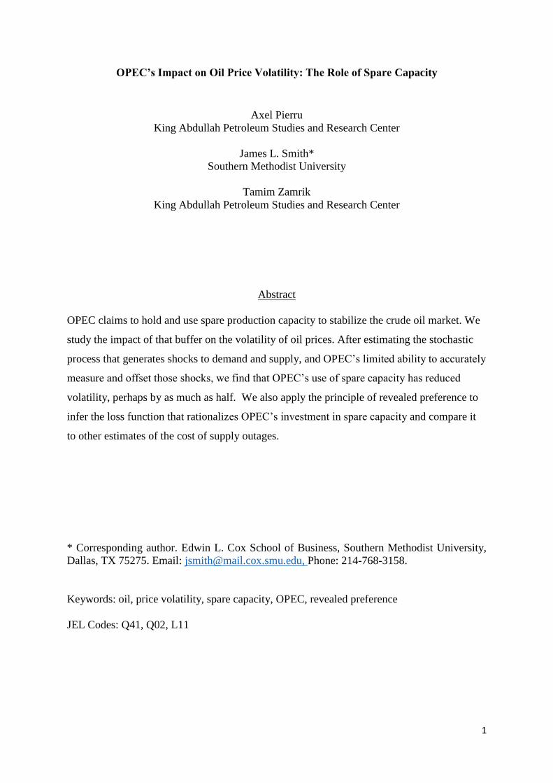
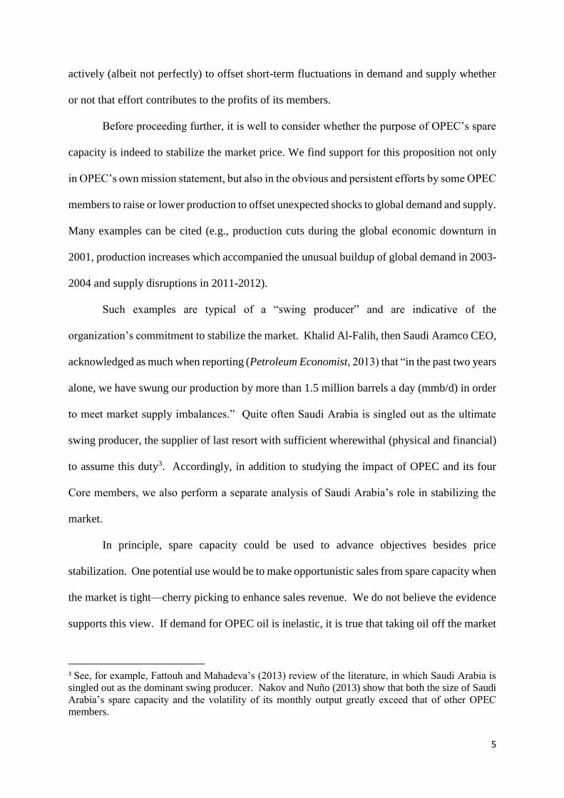
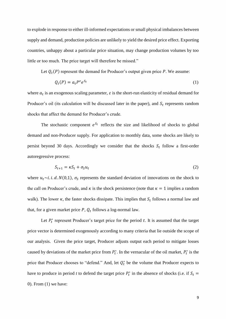
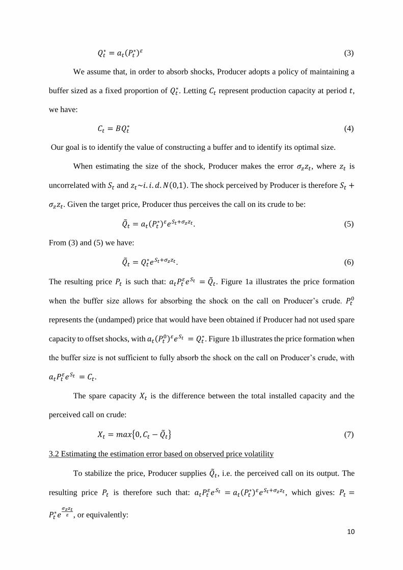
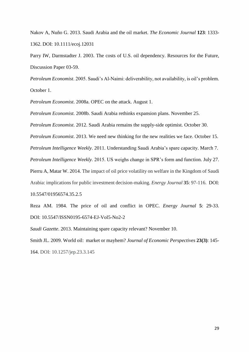
The resulting price 𝑃𝑡 is such that: 𝑎𝑡𝑃𝑡𝜀𝑒𝑆𝑡 = �̃�𝑡. Figure 1a illustrates the price formation

when the buffer size allows for absorbing the shock on the call on Producer’s crude. 𝑃𝑡0

represents the (undamped) price that would have been obtained if Producer had not used spare

capacity to offset shocks, with 𝑎𝑡(𝑃𝑡0)𝜀𝑒𝑆𝑡 = 𝑄𝑡

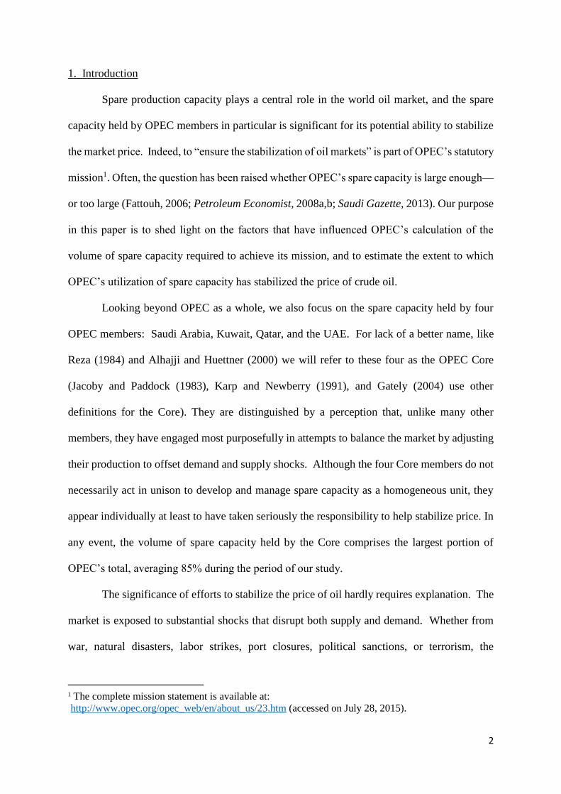
∗. Figure 1b illustrates the price formation when

the buffer size is not sufficient to fully absorb the shock on the call on Producer’s crude, with

𝑎𝑡𝑃𝑡𝜀𝑒𝑆𝑡 = 𝐶𝑡.

The spare capacity 𝑋𝑡 is the difference between the total installed capacity and the

perceived call on crude:

𝑋𝑡 = 𝑚𝑎𝑥{0, 𝐶𝑡 − �̃�𝑡} (7)

3.2 Estimating the estimation error based on observed price volatility

To stabilize the price, Producer supplies �̃�𝑡, i.e. the perceived call on its output. The

resulting price 𝑃𝑡 is therefore such that: 𝑎𝑡𝑃𝑡𝜀𝑒𝑆𝑡 = 𝑎𝑡(𝑃𝑡

∗)𝜀𝑒𝑆𝑡+𝜎𝑧𝑧𝑡, which gives: 𝑃𝑡 =

𝑃𝑡∗𝑒

𝜎𝑧𝑧𝑡𝜀 , or equivalently:

11

𝑙𝑛(𝑃𝑡) = 𝑙𝑛(𝑃𝑡∗) +

𝜎𝑧𝑧𝑡

𝜀 (8)

In other words, in the absence of outages, the deviation of the oil price from the target price is

attributable to the estimation error. We will therefore use the observed price volatility to

estimate the observation error. The conventional measure of volatility, 𝑣𝑜𝑙, is based on the

variance of returns (percentage change in price). From (8) we therefore have:

𝑣𝑜𝑙2 = 𝑣𝑎𝑟 [ln (𝑃𝑡

𝑃𝑡−1)] = 𝜎𝑇𝑃

2 + 2 (𝜎𝑧

𝜀)

2

(9)

The first term in this expression is the variance of the periodic percentage changes in Producer’s

target price: 𝜎𝑇𝑃2 = 𝑣𝑎𝑟 (𝑙𝑛 (

𝑃𝑡∗

𝑃𝑡−1∗ )). Solving (9) for the standard deviation of Producer’s

estimation error gives:

𝜎𝑧 =|𝜀|

√2√𝑣𝑜𝑙2 − 𝜎𝑇𝑃

2 (10)

Assuming that 𝜎𝑇𝑃2 = 0 therefore provides an upper bound on 𝜎𝑧. Of course, the term 𝜎𝑇𝑃

2

would vanish if the target price were increasing by a constant percentage each month. Upon

reviewing the development of the crude oil market during our sample period, it may not be

unreasonable4 to assume 𝜎𝑇𝑃2 ≅ 0. This assumption, along with an estimate of the residual

demand elasticity, allows us to approximate the standard deviation of Producer’s estimation

error:5

�̂�𝑧 = 𝑣𝑜𝑙 ×|𝜀|

√2 (11)

For our purposes, we use the average monthly Brent crude oil spot price series

published by the U.S. Energy Information Administration and estimate 𝑣𝑜𝑙 as the standard

4 After allowing for the disruption caused by the 2008/2009 financial crisis, the change in annual

average oil price shows an underlying trend that suggests that the target price may have been rising

fairly steadily over time. 5 Let 𝜆 measure the portion of observed volatility due to changes in the target price. Thus, 𝜎𝑇𝑃

2 = 𝜆 ×

𝑣𝑜𝑙2, in which case (11) takes the general form: �̂�𝑍 = 𝑣𝑜𝑙 ×|𝜀|

√2× √1 − 𝜆. As we show later, however,

our main results and conclusions are robust with respect to the presumed value of 𝜆.

12

deviation of the log-returns of the average monthly price over our sample period (which goes

from September 2001 to October 2014). This gives 𝑣𝑜𝑙 = 8.58%.

𝜀, the short-run (monthly) elasticity of residual demand for Producer’s oil, is by

construction equal to [𝜀𝐷 − (1 − 𝜌)𝜀𝑆]/𝜌, where 𝜀𝐷 and 𝜀𝑆 represent the short-run elasticity of

global demand and non-Producer supplies, and 𝜌 is the Producer’s market share of global

output.

Our estimation procedure is therefore sensitive to 𝜀𝐷 and 𝜀𝑆, the presumed elasticities

of demand and non-Producer supply. Given the range of estimates found in the literature, our

analysis will be subjected to sensitivity analysis. The literature traditionally sees both global

demand and non-OPEC supply to be highly inelastic in the short-run. Hamilton (2009)

proposed a short-run global demand elasticity of -0.06, but noted that it might be higher or

lower. Based on observed price movements following specific disruptions of the market, Smith

(2009) suggested short-run demand and supply elasticities of 0.05 and 0.05, which together

produce a “ten-times” multiplier that translates physical outages into price spikes. Baumeister

and Peersman (2013) provide corroborating evidence based on a time-varying parameter vector

autocorrelation analysis of global crude oil demand and supply. Their estimates of the quarterly

demand elasticity fall between 0.05 and 0.15 throughout our sample period, and their

estimates of the quarterly supply elasticity are of the same magnitude. Because our data are

monthly, we consider a global demand elasticity ranging from -1% to -5% to be consistent with

this literature (for values within this range we take 𝜀𝑆 = |𝜀𝐷|). Kilian and Murphy (2014) derive

a much higher estimate of the short-run elasticity of demand (0.26) from a structural vector

autoregression that takes into account estimated monthly changes in the global volume of

speculative crude oil inventories. Therefore, we also include a sensitivity case where the

monthly demand elasticity is 0.26 and the monthly supply elasticity is 0, per Kilian and

Murphy.

13

For each group of producers, we compute the average crude oil supply per month and

global market share over the sample period. Our crude oil supply data are from the IEA

Monthly Oil Data Service; production from the Neutral zone is not included in Saudi

production (but included in OPEC Core production); for OPEC, we use the “OPEC Historical

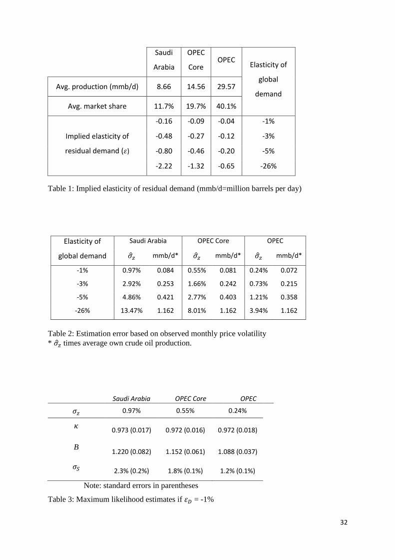
Composition” series. Table 1 provides the implied elasticities of residual demand. Table 2

provides the corresponding standard deviation of the estimation error, in both relative and

absolute terms, calculated from (11). The absolute estimation errors (barrels per day) attributed

to Saudi Arabia, the Core, and OPEC are roughly equal in size. The values range between 0.07

and 1.16 mmb/d, with all values below or equal to 0.4 mmb/d if global demand elasticity does

not exceed -5%, which appears sensible to us. Since Saudi production is smaller than that of

the Core, which in turn is smaller than that of OPEC, the relative size of the error (% of

producer's output) respectively decreases, as shown in Table 2.

The precision of �̂�𝑧 can be estimated using the Chi-Square distribution. A 95%

confidence interval for 𝜎𝑧2 is given by: [

(𝑛−1)�̂�𝑧2

𝐾.975,

(𝑛−1)�̂�𝑧2

𝐾.025], where 𝐾.975 and 𝐾.025 are cutpoints

from the Chi-Square distribution with 𝑛 − 1 degrees of freedom. Based on the 158 monthly

observations in our sample, the 95% confidence interval for 𝜎𝑧 is: [0.901�̂�𝑧 , 1.124�̂�𝑧].

3.3 Estimation of other parameters based on spare capacity

Because 𝐶𝑡 = �̃�𝑡 + 𝑋𝑡, after using (4) and (6) to substitute for 𝐶𝑡, we have:

−𝑙𝑛 (1 +𝑋𝑡

�̃�𝑡) = 𝑆𝑡 + 𝜎𝑧𝑧𝑡 − 𝑙𝑛(𝐵) (12)

The left-hand side of (12) is observable. The right-hand side represents the perceived

autoregressive shocks to Producer’s demand (cf. (2)) with unknown parameters 𝐵 (buffer size),

𝜎𝑆 (volatility of demand shocks), and 𝜅 (shock persistence). Given monthly data on actual

production and spare capacity, along with our previous estimate of 𝜎𝑧, maximum likelihood

estimates of 𝐵, 𝜎𝑆, and 𝜅, along with the covariance matrix, are obtained by the procedure

14

described in Appendix 1. We here ignore the data censoring represented by (7) which occurs

whenever the shock exceeds the size of the buffer capacity (i.e., when there is an outage).

However this should not matter since in our sample only the Saudi data exhibit spare capacity

equal to zero (during three months only). The historical monthly frequency of outage is

therefore very low (1.9% for Saudi Arabia, zero for OPEC and OPEC Core), which simply

reflects the fact that the spare capacity has almost always been sufficient to meet the perceived

call on production. This remark also applies to the previous section where we attribute all the

price volatility to the observation error.

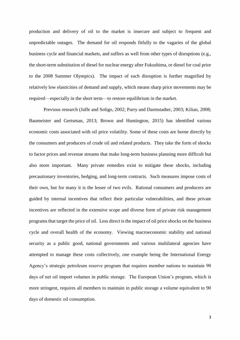
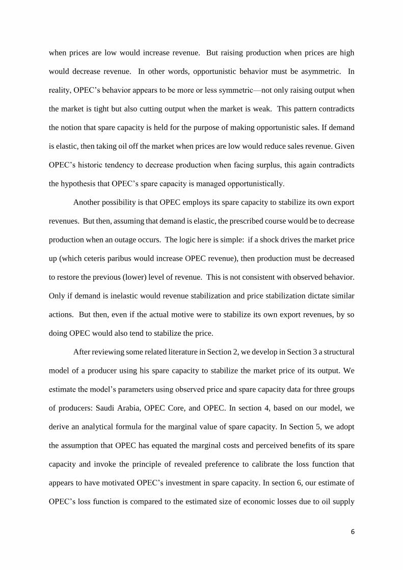
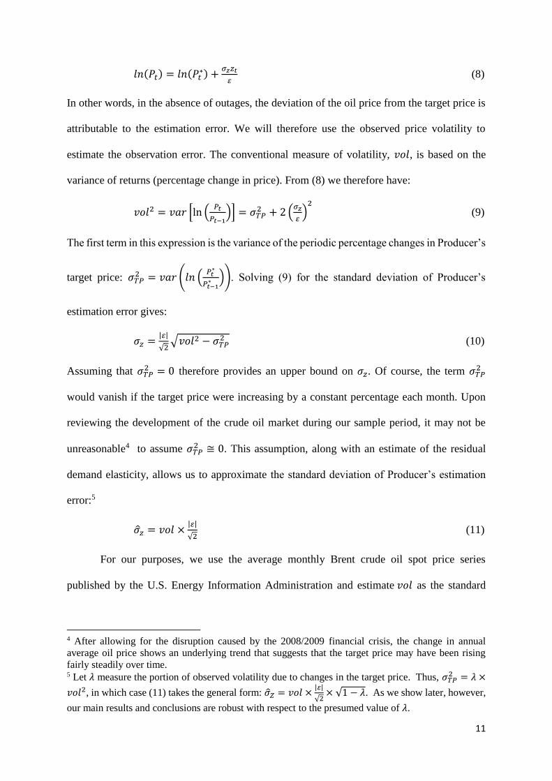
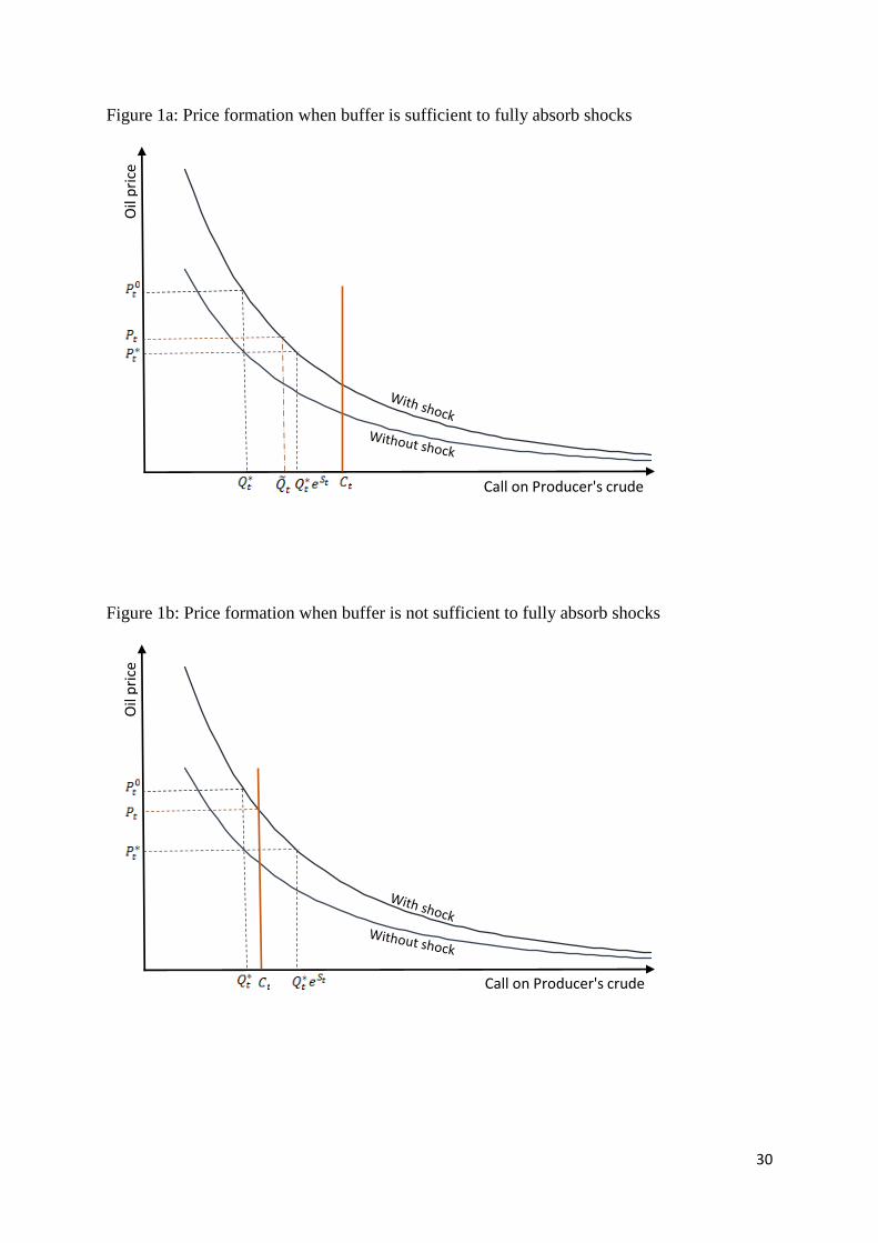
Figure 2 shows the monthly variation in reported spare capacity of OPEC, Saudi Arabia,

and the OPEC Core. Our data come from the International Energy Agency (IEA) and represent

what the IEA calls “effective” spare capacity.6 The monthly spare capacity data for Saudi

Arabia and OPEC were provided directly by IEA in an Excel file7. To build the series for the

OPEC Core, we collected8 the data for Kuwait, UAE and Qatar from monthly issues of IEA’s

Oil Market Report. Because spare capacities are not reported on a regular basis prior to

September 2001, our sample extends from September 2001 to October 2014 (158 observations

for each series). These are the primary data with which we estimate the stochastic process

governing shocks to the call on OPEC production. The estimates and their standard errors are

reported in Table 3 for the case where the global demand elasticity is assumed to be -0.01. The

estimates and standard errors corresponding to the other elasticity cases are nearly identical to

6 According to the IEA, spare capacity is defined as “capacity levels that can be reached within 30 days

and sustained for 90 days.” Effective spare capacity captures the difference between nominal capacity

and the fraction of that capacity actually available to markets (Munro, 2014). 7 Email from Steve Gervais (IEA) on January 7th, 2015. 8 We had five missing data for the non-Saudi members of OPEC Core. We consider that, because of a

typo, the values for November 2002 and 2010 are those reported for October in the December’s Oil

Market Report (as these values differ from those reported for October in the November’s report). The

three other missing data are for June 2002, April 2003 and March 2007. We interpolate the missing

values with the formula: 𝑋𝑐,𝑡 = 𝑋𝑆,𝑡 +𝑋𝑂,𝑡−𝑋𝑆,𝑡

2[

𝑋𝐶,𝑡−1−𝑋𝑆,𝑡−1

𝑋𝑂,𝑡−1−𝑋𝑆,𝑡−1+

𝑋𝐶,𝑡+1−𝑋𝑆,𝑡+1

𝑋𝑂,𝑡+1−𝑋𝑆,𝑡+1] , where 𝑋𝑆,𝑡, 𝑋𝑐,𝑡 and 𝑋𝑂,𝑡

represent the spare capacity of Saudi Arabia, OPEC Core and OPEC, respectively, in month t.

15

these and therefore remanded to the appendix.

The estimates for B, the size of the buffer, and 𝜎𝑆, the magnitude of the innovations on

the shock exhibit a common pattern: the greatest values are obtained for Saudi Arabia, and the

lowest for OPEC. This is consistent with the (traditional) view that Saudi Arabia is the swing

producer and absorbs more shocks than the other OPEC producers (relatively to the size of the

residual demand for its crude). In all cases, the estimated size of the Saudi buffer is about 21%

of the expected call on Saudi Arabia’s output, whereas for the Core (15%) and OPEC as a

whole (9%) it is smaller.

To better understand the absolute size of the estimated buffers, we first determine 𝑄∗,

the average call on Producer’s crude in the absence of shocks. 𝑄∗ is the average of 𝑄𝑡∗ =

�̃�𝑡+𝑋𝑡

𝐵.

For an elasticity of global demand of -1%, this gives 𝑄∗ = 8.82 mmb/d for Saudi Arabia, 14.91

mmb/d for the Core, and 30.02 for OPEC as a whole. The average size of the buffer in absolute

terms is then calculated by multiplying 𝑄∗ by 𝐵 − 1. As one would expect, the larger is the

group of countries, the bigger is the average size of the buffer: 1.94 mmb/d for Saudi Arabia,

2.27 mmb/d for OPEC Core, and 2.64 mmb/d for OPEC. The Saudi figure is consistent with

the various official pronouncements that have emanated from the Kingdom, which says their

intended buffer has ranged between 1.5 and 2 mmb/d (see for instance Petroleum Economist

(2005, 2012) and H.E. Ali Al-Naimi’s address at CERAWeek (2009) and remarks at the 12th

International Energy Forum (2010)). When considering the estimated speed at which shocks

dissipate (Table 3), the estimated half-life is roughly 25 (𝜅 = 0.973) months. Although the

differences in the estimated 𝜅 appear small and are not statistically significant across all the

elasticity cases, the implied half-life is considerably shorter (15 months) for the case of -0.26

demand elasticity (see appendix).

16

4. Incremental value of spare capacity

We assume that Producer incurs costs in any period when the perceived call exceeds

production capacity. Such outages are denoted by 𝑂𝑡 ≝ 𝑚𝑎𝑥{0, �̃�𝑡 − 𝐶𝑡}. The outage equals

the portion of the call that Producer is not able to meet. From (4), (6) and (7), the outage can

be written equivalently as 𝑂𝑡 = 𝑚𝑎𝑥{0, (𝑒𝑆𝑡+𝜎𝑧𝑧𝑡 − 𝐵)𝑄𝑡∗}. An outage occurs whenever the

perceived shock exceeds the size of the buffer.

The probability of an outage depends on the size of the buffer and is given by:

𝜑𝑡(𝐵) ≝ 𝑝𝑟(𝑂𝑡 > 0|𝐵) = ∫ 𝑔𝑡(𝜉)∞

𝑙𝑛(𝐵)𝑑𝜉 (13)

where 𝑔𝑡(. ) represents the marginal density of 𝑆𝑡 + 𝜎𝑧𝑧𝑡 based on the information set at time

𝑡 = 0.

The expected size of the outage is:

𝐸[𝑂𝑡|𝐵] = ∫ (𝑒𝜉 − 𝐵)𝑄𝑡∗𝑔𝑡(𝜉)𝑑𝜉

∞

𝑙𝑛(𝐵) (14)

whereas the conditional expectation, given that an outage occurs, is:

𝐸[𝑂𝑡|𝐵 ∩ 𝑂𝑡 > 0] = 𝐸[𝑂𝑡|𝐵]

𝜑𝑡(𝐵) (15)

We postulate a quadratic loss function that reflects the present value of Producer’s

damages that result from all future outages:

𝐿 = 𝛼 ∑(𝑂𝑡)2

(1+𝑟)𝑡𝑇𝑡=1 (16)

where 𝑟 is the real risk-adjusted periodic discount rate and 𝛼 is a latent preference parameter

that reflects the weight that Producer attaches to outages. The loss function is increasing in the

square of the size of individual outages and additive regarding their occurrence. The planning

horizon is defined by 𝑇. We treat 𝑇 as the service life of a designated production facility kept

for spare. The value of the buffer to Producer is determined by its ability to reduce the expected

loss resulting from outages. As shown in Appendix 3, the incremental value, 𝑣, of spare

capacity is given by:

17

𝑣 = −𝜕𝐸[𝐿|𝐵]

𝜕𝐵= 2𝛼 ∑

𝐸[𝑂𝑡|𝐵]𝑄𝑡∗

(1+𝑟)𝑡𝑇𝑡=1 (17)

Note that the value of expanding the buffer does not depend on the functional form of 𝑔𝑡(. ),

only on 𝐸[𝑂𝑡|𝐵], which is itself the product of 𝜑𝑡(𝐵) (the probability of an outage) and

𝐸[𝑂𝑡|𝐵 ∩ 𝑂𝑡 > 0], as well as the length of the planning horizon, the expected call, and 𝛼. In

the next section, we show how all of these parameters can be estimated from existing data. Of

particular interest is the estimated value of 𝛼 because that will allow us to calibrate Producer’s

loss function and compare the cost of outages as perceived by Producer (whether OPEC, OPEC

Core, or Saudi Arabia) to independent estimates of the global economic cost of outages. That

comparison, in turn, will provide an indication of the extent to which OPEC’s stabilization

policy addresses the interests of the global economy.

As shown in Appendix 3, an immediate implication of (17) is that the expected loss and

the value of incremental spare capacity are both decreasing in the size of the buffer. To evaluate

(17), we shall need to calculate:

𝐸[𝑂𝑡|𝐵] = 𝑄𝑡∗(𝐸[𝑒𝑆𝑡+𝜎𝑧𝑧𝑡|𝑆𝑡 + 𝜎𝑧𝑧𝑡 > 𝑙𝑛(𝐵)] − 𝐵) × 𝜑𝑡(𝐵) (18)

Since we are considering a long-term policy of maintaining a buffer of optimal size, we will

use the covariance-stationary process that satisfies (2) (see Hamilton (1994) p. 53). 𝑆𝑡 + 𝜎𝑧𝑧𝑡

therefore follows a normal law with mean zero and variance 𝜎2 = 𝜎𝑧2 +

𝜎𝑆2

1−𝜅2. We make the

additional assumption that the call on Producer’s crude in the absence of shocks remains stable

and equal to 𝑄∗.

We now use the following fact about the mean of a truncated lognormal distribution

(Johnson et al., 1994, p.241):

𝐸[𝑒𝑆𝑡+𝜎𝑧𝑧𝑡|𝑆𝑡 + 𝜎𝑧𝑧𝑡 > 𝑙𝑛(𝐵)] = 𝑒 𝜎2 2⁄ Φ(σ−𝑙𝑛(𝐵) 𝜎⁄ )

𝜑(𝐵) (19)

where: 𝜑(𝐵) = 1 − Φ(ln(B) σ⁄ ) and where Φ(∙) represents the cumulative distribution of the

standard normal law.

18

From (14) we therefore have:

𝐸[𝑂𝑡|𝐵] = 𝑄∗ (𝑒𝜎2 2⁄ Φ (σ −𝑙𝑛(𝐵)

𝜎) − 𝐵 (1 − Φ (

ln(𝐵)

𝜎))) (20)

Upon substituting (20) into (17), we obtain the parametric form of the incremental value

of spare capacity:

𝑣 = (𝑒𝜎2 2⁄ Φ (σ −𝑙𝑛(𝐵)

𝜎) − 𝐵 (1 − Φ (

ln(𝐵)

𝜎))) ∑

2𝛼(𝑄∗)2

(1+𝑟)𝑡𝑇𝑡=1 (21)

5. Revealed Preference for Spare Capacity

We now show how (21) and the principle of revealed preference can be used to infer

the value of 𝛼, the behavioral parameter that reveals how much importance Producer attaches

to outages.

Denote by ℎ the marginal cost to provide 1 barrel per day of additional spare capacity.

This is the capital expenditure to construct the capacity, plus maintenance cost, less any net

revenue generated when that incremental barrel of spare capacity is used. If it is known that the

cost is 𝐾 to construct a production facility with peak production rate 𝑅, then the capital cost

per daily barrel of spare capacity is given by 𝑘 = 𝐾/𝑅. In addition, for the additional spare

capacity we have to account for the periodic maintenance costs (which are incurred even when

spare capacity is not in use) and net financial gains (which are generated only when barrels are

released from spare capacity). Any release generates marginal revenue that may be either

positive or negative depending on the elasticity of residual demand. The net financial gain from

each release is the marginal revenue minus the operating cost of producing the barrel. Over the

life of the facility, the present value of the periodic maintenance costs is represented by 𝑚,

while the present value of expected net financial gains is represented by 𝑓. Therefore, from

the Producer’s perspective the present value of total outlay for an incremental barrel of spare

capacity is ℎ = 𝑘 + 𝑚 − 𝑓.

19

If, consistent with the principle of revealed preference, we assume the historical size of

the buffer has been optimized, then the marginal cost of the buffer must equal the incremental

benefit. Since 𝑣 is derived for a buffer defined in relative terms, at the optimized buffer size

we must have: ℎ𝑄∗ = 𝑣,9 which implies:

𝑘 + 𝑚 − 𝑓 = (𝑒𝜎2 2⁄ Φ (σ −𝑙𝑛(𝐵)

𝜎) − 𝐵 (1 − Φ (

𝑙𝑛(𝐵)

𝜎))) ∑

2𝛼𝑄∗

(1+𝑟)𝑡𝑇𝑡=1 (22)

A rational agent therefore sizes the buffer based on four factors: the size and frequency

of shocks to demand, the precision with which agent can estimate those shocks, the importance

attached to resulting outages (as represented by the parameter 𝛼 of the loss function), and the

cost of developing, maintaining, and operating spare capacity (including potential financial

gains or losses). Given the estimated size of the buffer, (22) allows us to infer the loss function

that would rationalize OPEC’s investment in spare capacity:

𝛼 =𝑘+𝑚−𝑓

(𝑒𝜎2 2⁄ Φ(σ−𝑙𝑛(𝐵)

𝜎)−𝐵(1−Φ(

ln(𝐵)

𝜎))) ∑

2𝑄∗

(1+𝑟)𝑡𝑇𝑡=1

(23)

To investigate this issue empirically, the call on Producer’s crude in the absence of

shocks (𝑄∗) is estimated using the average values calculated previously in Section 3.3. We

have previously discussed all other parameter estimates that appear in the denominator of (23),

and now turn to the cost parameters in the numerator. The spare capacity that exists within

OPEC can be drawn from many sources, including increased liftings from producing fields as

well as additional production from idle facilities (if any). We assess the costs associated with

incremental production via the simplifying assumption that it all comes from a dedicated buffer

facility that is reserved for that specific purpose. Although this may depart somewhat from

9 ℎ = 𝑘 + 𝑚 − 𝑓 represents the cost of expanding the buffer by one barrel per day, which on average

corresponds to 1/𝑄∗ in percentage terms, whereas 𝑣 represents the benefit from expanding the buffer

by 1 percent.

20

reality, it provides a useful proxy for the more complicated and diffuse costs that may actually

be incurred.

The capital cost of spare capacity (𝑘) can be estimated using data from the most recent

oil field development in Saudi Arabia, the Manifa field that is located in a shallow offshore

setting. According to Henni (2013), the total capital cost to develop Manifa’s production

capacity of 900,000 barrels per day (which corresponds to our parameter 𝑅) is $15.8 billion

(which corresponds to our parameter 𝐾). Therefore, the capital cost per daily barrel of

production capacity is given by 𝑘 = 𝐾 𝑅⁄ =$17,500.

We assume that the maintenance cost remains constant throughout time and take it from

QUE$TOR, IHS’s cost estimating software package that is a petroleum-industry standard. For

an idle facility located in Saudi Arabia with 40 wells and combined production capacity of

200,000 barrels per day, QUE$TOR estimates annual maintenance cost to be $410 per daily

barrel, or $34.167 on a monthly basis. Thus, for an annual real discount rate of 4% in line with

Pierru and Matar’s (2014) findings for Saudi Arabia, the present value of maintenance costs

over the 240-month life of the facility (which corresponds to our parameter 𝑚) would be:

∑34.17

(1.04)𝑡

12

240𝑡=1 , which gives 𝑚 = $5,670 per daily barrel of capacity.

The incremental barrel of buffer capacity would only be used when there is an outage.

For each group of producers, we consider the average price ($45.24 per barrel) observed during

the three Saudi outage months (from August to October 2004) and use that price (along with

the usual formula for marginal revenue) to determine the parameter 𝑓 as the sum of expected

monthly net financial gains over the 240-month life of the facility discounted at 4%, assuming

$2 production cost per barrel10. We thus have:

10 Petroleum Intelligence Weekly (2011) reports Saudi Aramco’s group-wide average production cost

as falling between $2.00 and $3.00 per barrel. Also note that we assume that the marginal revenue is

received for each of thirty days within any month affected by an outage.

21

𝑓 = ∑

𝜑(𝐵)30 ((1 +1𝜀) 45.24 − 2)

(1.04)𝑡

12

240

𝑡=1

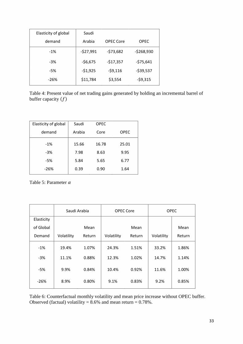
The resulting estimates of the financial gains due to an incremental barrel of buffer are given

by Table 4. 𝑓 is negative when the residual demand is inelastic.

6. Assessment and discussion of the implicit loss function

After substituting the parameter estimates discussed above into (23), we obtain the

estimated values of 𝛼 shown in Table 5. These values represent the inferred weight that

Producer attaches to outage events.

Using the estimated values of 𝛼, it is possible to evaluate the loss function that

rationalizes Producer’s choice of the buffer. Consider, for example, OPEC Core, for whom the

expected size of an outage (when one occurs) is roughly half a million barrels per day.11 By

substituting the estimated values of 𝛼 from Table 5 into the loss function (16), we can calculate

the cost that the Core attaches to an outage of half a million barrels per day that lasts for 6

months. We get a cost of $24.87 billion if the elasticity of global demand is assumed to be

1%, $12.80 billion if elasticity is 3%, $8.38 billion if elasticity is 5%, and $1.34 billion if

elasticity is 26%.

These results mean little when standing alone, but are of considerable interest when

compared to other informed estimates of the economic cost that such an outage would impose

on the global economy. For this purpose, we have applied Oxford Economics Global

Economic Model to simulate the impact on global GDP of outages of varied size and duration.

Appendix 4 provides the information on the model and the procedure we followed, and the

11 From (15) and (20) we derive the expression of the (conditional) expected outage size:

𝐸[𝑂𝑡|𝐵 ∩ 𝑂𝑡 > 0] = 𝑄∗

𝜑(𝐵)(𝑒𝜎2 2⁄ Φ(σ − ln (𝐵) 𝜎⁄ ) − 𝐵𝜑(𝐵)). For OPEC Core this gives a size

ranging between 0.50 and 0.53 mmb/d when global demand elasticity is lower or equal to -5% (0.82

mmb/d when elasticity is -26%).

22

results obtained are given in Table A4. According to the Oxford Economics model, a six-month

outage of 0.5 mmb/d that is assumed to occur at the beginning of 2015 would reduce the present

value of global GDP over the next five years by some $22.36 billion, relative to the reference

scenario. This loss lies near the top of the range of perceived costs that we believe the OPEC

Core may have attributed to such an outage. Similar results hold for Saudi Arabia and for

OPEC as a whole.

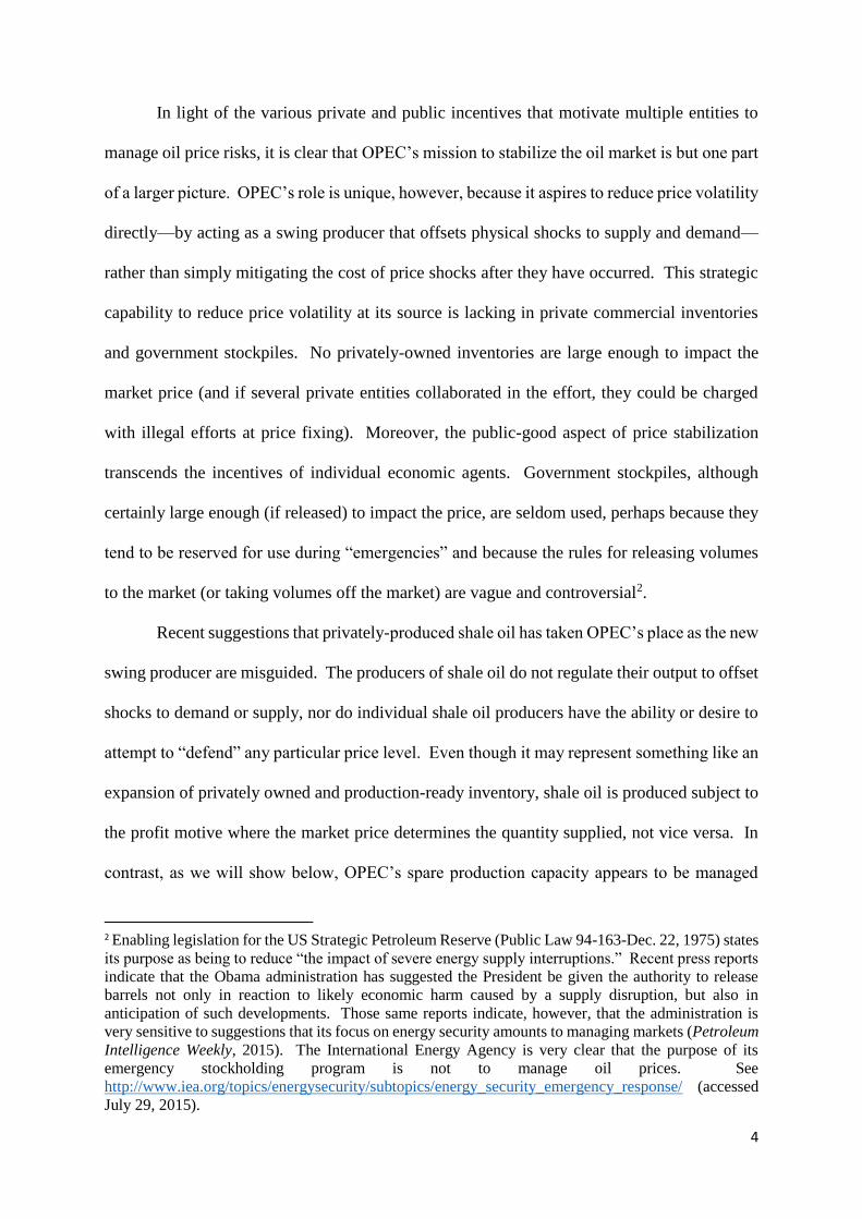
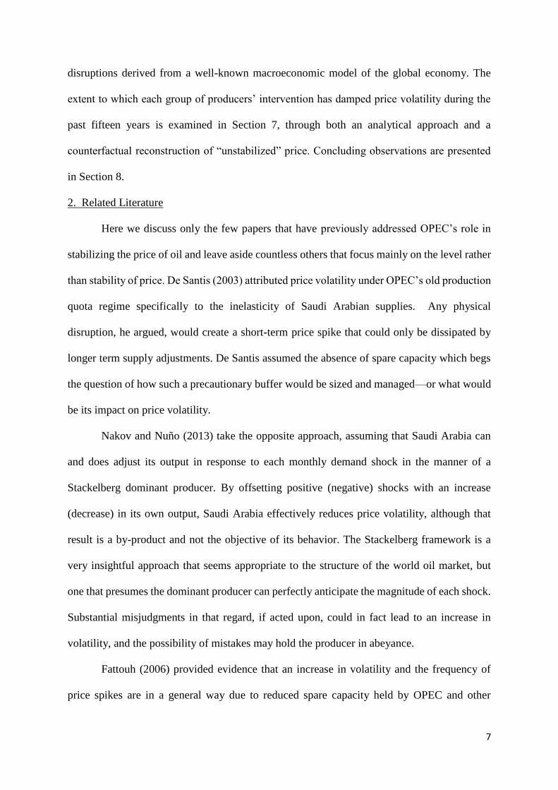
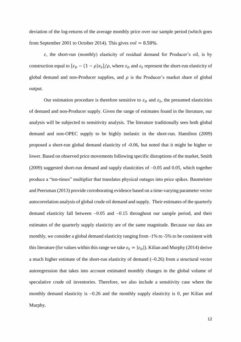
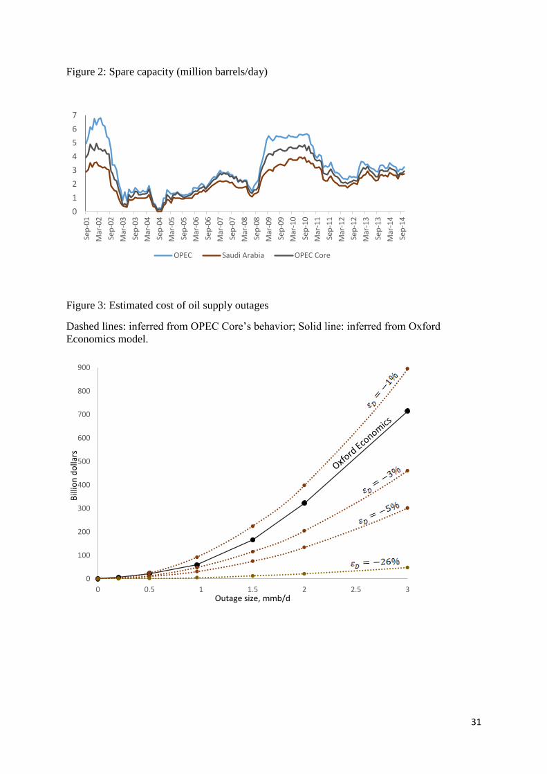
For differently sized six-month outages, Figure 3 compares the global cost inferred

from the Oxford Economics model and the inferred cost that rationalizes OPEC Core’s choice

of buffer (assuming different values for elasticity of global oil demand). Even if global demand

is assumed to be relatively elastic in the short term (-5%), the costs that rationalize OPEC

Core’s buffer comprise 40% of the “global” costs. This does not imply that the buffer is too

small, only that the OPEC Core may for whatever reason be motivated12 to address only a

portion of the damage caused by oil shocks. We repeat an earlier point: the OPEC Core is but

one piece of a much larger picture when it comes to neutralizing the impact of oil shocks.

Whether it is reasonable to believe that 60% of the burden should be left for individual

consumers, producers, government agencies, and multilateral organizations, (not to mention

the other members of OPEC) to deal with, we are unable to say. We leave that debate to others.

However, if global demand is assumed to be highly inelastic in the short term (-1%), the costs

that rationalize the size of the Core’s buffer actually exceed the level of global costs projected

by the Oxford Economics model.

12 Note that whatever motivated OPEC Core’s decision to build its observed buffer, that decision has

sheltered the global economy from potential outages. Let us for instance consider 𝜀𝐷 = −5%.

According to (19) and (20), if there had been no buffer (𝐵 = 1), the outage probability and conditional

expected size would have increased from 3.3% to 50% and from 0.53 mmb/d to 1.09 mmb/d,

respectively.

23

7. The Impact of Spare Capacity on Price Volatility

We evaluate the counterfactual price, 𝑃𝑡0, that would have been obtained if Producer

had produced 𝑄𝑡∗ instead of using spare capacity to offset shocks:

𝑎𝑡(𝑃𝑡0)𝜀𝑒𝑆𝑡 = 𝑎𝑡(𝑃𝑡

∗)𝜀

It follows that:

𝑙𝑛 (𝑃𝑡

0

𝑃𝑡−10 ) = 𝑙𝑛 (

𝑃𝑡∗

𝑃𝑡−1∗ ) +

𝑆𝑡−1−𝑆𝑡

𝜀 ,

which implies:

𝑣𝑎𝑟 (𝑙𝑛 (𝑃𝑡

0

𝑃𝑡−10 )) = 𝜎𝑇𝑃

2 +1

𝜀2 𝑣𝑎𝑟(𝑆𝑡 − 𝑆𝑡−1) (24)

The covariance stationary process satisfying (2) is such that:

𝑣𝑎𝑟(𝑆𝑡) = 𝑣𝑎𝑟(𝑆𝑡−1) =𝜎𝑆

2

1−𝜅2, with 𝑐𝑜𝑣(𝑆𝑡, 𝑆𝑡−1) =𝜅𝜎𝑆

2

1−𝜅2. Eq. (24) therefore gives:

𝑣𝑎𝑟 (𝑙𝑛 (𝑃𝑡

0

𝑃𝑡−10 )) = 𝜎𝑇𝑃

2 +2𝜎𝑆

2

(1+𝜅)𝜀2 (25)

Producer’s action stabilizes the price if 𝑣𝑎𝑟 (𝑙𝑛 (𝑃𝑡

0

𝑃𝑡−10 )) > 𝑣𝑎𝑟 (ln (

𝑃𝑡

𝑃𝑡−1)). According to (9)

and (25), this will occur if and only if:

2𝜎𝑆2

(1 + 𝜅)𝜀2>

2𝜎𝑧2

𝜀2

This requires:

𝜎𝑆2 > (1 + 𝜅)𝜎𝑧

2 (26)

This condition highlights the fact that the Producer’s ability to stabilize the price

depends only on the precision of its estimate relative to the volatility and persistence of shocks;

it does not depend on the elasticity of demand. Our estimate of the precision of Producer’s

estimate, however, is conditioned on the presumed elasticity, as shown in Table 2. Condition

(26) therefore appears to be satisfied under certain of our elasticity scenarios (e.g., Saudi Arabia

24

and OPEC Core when the price elasticity of global demand is presumed to be -1%, and for

OPEC when the elasticity is presumed to be -1% or -3%), but not in others (see Table 3 and

Appendix Tables A1-A3).

We now conduct an independent counterfactual experiment to examine the actual

impact that Producer’s utilization of spare capacity has had on price volatility over our sample

period. This counterfactual experiment does not use any of our previous estimates or results.

If Producer were content to produce only to meet its expected call, 𝑄𝑡∗, then the quantity

�̃�𝑡+𝑋𝑡

𝐵,

instead of �̃�𝑡, would have been put on the market in each period. The counterfactual price must

therefore satisfy:

𝑎𝑡(𝑃𝑡0)𝜀𝑒𝑆𝑡 =

�̃�𝑡 + 𝑋𝑡

𝐵

After substituting for 𝑎𝑡𝑒𝑆𝑡 using 𝑎𝑡𝑃𝑡𝜀𝑡𝑒𝑆𝑡 = �̃�𝑡, this gives:

𝑙𝑛 (𝑃𝑡

0

𝑃𝑡−10 ) = 𝑙𝑛 (

𝑃𝑡

𝑃𝑡−1) +

1

𝜀𝑙𝑛 (1 +

𝑋𝑡

�̃�𝑡) −

1

𝜀𝑙𝑛 (1 +

𝑋𝑡−1

�̃�𝑡−1) (27)

Conditional on the presumed elasticity of demand, which is the only unobservable

variable on the right-hand side, the volatility and trend of the counterfactual price series can be

calculated from (27). The results are given in Table 6.

All the counterfactual volatilities exceed the historical volatility of 8.58%, which is to

say that it appears OPEC’s utilization of spare capacity has damped price movements. This

indicates that condition (26) must be satisfied in practice. It also casts doubt on the presumption

that the short-run elasticity of global demand deviates much from zero, since values that exceed

|𝜀𝑑| = 0.03 produce estimates of 𝜎𝑧 that fail condition (26), which would be a contradiction of

Table 6.13 Our counterfactual experiment does not, of course, reveal the true identity of the

13 Even if we treat the reported values of 𝜎𝑍 as upper bounds on the estimation error and factor out the

contribution due to volatility of the target price, per footnote 5, the adjusted estimates of 𝜎𝑍 would still

violate condition (26) and contradict the results shown in Table 6 unless the elasticity of global demand

is close to zero. We note that Nakov and Nuño (2013) experience similar difficulty simulating historical

price and output volatilities when a high demand elasticity (0.26) is imposed on their model.

25

“Producer” whose actions have succeeded in stabilizing the market, be it Saudi Arabia, the

Core, or OPEC acting all together. Based on other evidence, however, one may doubt that

OPEC as a whole has played this role. Many OPEC members are reported to produce

continuously at full capacity. Whether it has been Saudi Arabia or the OPEC Core acting as

swing producer makes little difference, at least according to the estimates shown in Table 6.

The counterfactual volatilities and trends are similar in both scenarios. Our estimates indicate

that Saudi/Core intervention has damped oil price volatility by some 23% to 30% if the monthly

elasticity of global demand is thought to be -0.03, or by 56% to 65% if the elasticity is thought

to be -0.01.14 Differences in assumptions regarding the elasticity of global demand and non-

OPEC supply translate into big differences regarding the extent to which OPEC appears to

have stabilized the market price. One’s view of the impact of OPEC’s efforts to stabilize the

price clearly runs inversely to one’s opinion about short-run elasticities of demand and supply,

which makes the elasticity a worthy subject of further research.

8. Concluding remarks

We believe the present paper is the first attempt to fit a structural model to the behavior

of OPEC’s spare capacity. Although discussions of oil price dynamics frequently mention the

influence of this factor, as yet there has been no quantitative investigation of the determinants

of the size or impact of spare capacity. To that end, we have constructed a model having three

main components: an autoregressive stochastic process by which the residual demand for

OPEC oil is shocked, a separate stochastic process by which OPEC attempts to estimate the

size of such shocks and offset them by regulating production from its buffer stock, and finally,

a loss function which describes the benefits that rationalize the observed size of OPEC’s chosen

buffer—and which can be compared to independent assessments of the global economic cost

of oil supply disruptions.

14 The 23% reduction in volatility is calculated from Table 6 as (11.1%-8.6%)/11.1%, etc.

26

By estimating the parameters of this model using monthly data, we obtain plausible

results regarding the size and persistence of demand and supply shocks that impact the global

oil market, plausible estimates of the precision (or lack thereof) of OPEC’s ability to estimate

and offset shocks, and plausible estimates of the scope of OPEC’s concern for the economic

costs that oil price shocks impose on the global economy. We also perform a counterfactual

experiment to calculate the apparent impact of OPEC’s use of spare capacity during the past

fifteen years. Depending on one’s particular beliefs regarding the short-run elasticity of global

demand and supply for oil, OPEC’s impact may be viewed as large or small—but in all cases

having at least partially offset shocks and stabilized the price. Under plausible assumptions

regarding the elasticity of demand, OPEC’s stabilizing influence appears to have been very

substantial, with indications that Saudi Arabia may have acted as a supplier of last resort and,

relative to the size of the residual demand for its oil, absorbed more shocks than the other OPEC

members.

In this paper, we are abstracting from the impact of volatility on the formation of

production capacity outside OPEC and on fuel substitution in demand. In addition, our study

has focused on the past. There are many who would argue that OPEC has done little, of late,

to stabilize the price of oil in the short term. We do not deny the many indications of a strategic

change within OPEC in late 2014, following the end of our sample period. What remains to

be seen is whether the market, and OPEC’s role, has changed forever, or whether the market

will gradually adjust to a new equilibrium in which OPEC continues to pursue its goal of market

stabilization, albeit at a lower target price.

27

List of References

Alhajji AF, Huettner D. 2000. OPEC and world crude oil markets from 1973 to 1994: cartel,

oligopoly, or competitive? Energy Journal 21(3): 31-60. DOI: 10.5547/ISSN0195-6574-EJ-

Vol21-No3-2

Baumeister C, Peersman G. 2013. Time varying effects of oil supply shocks on the US

economy. American Economic Journal: Macroeconomics 5(4): 1-28. DOI: 10.1257/mac.5.4.1

Baumeister C, Peersman G. 2013. The role of time-varying price elasticities in accounting for

volatility changes in the crude oil market. Journal of Applied Econometrics 28: 1087-1109.

DOI: 10.1002/jae.2283

Brown S, Huntington HG. 2015. Evaluating U.S. oil security and import reliance. Energy

Policy 79(C): 9-22.

De Santis RA. 2003. Crude oil price fluctuations and Saudi Arabia’s behaviour. Energy

Economics 25: 155-173.

Difiglio C. 2014. Oil, economic growth and strategic petroleum stocks. Energy Strategy

Reviews 5: 48-58. DOI: 10.1016/j.esr.2014.10.004

Fattouh B. 2006. Spare capacity and oil price dynamics. Middle East Economic Survey 49(5).

Fattouh B, Mahadeva L. 2013. OPEC: what difference has it made? Oxford Institute for Energy

Studies, MEP 3.

Gately D. 2004. OPEC’s incentives for faster output growth. Energy Journal 25: 75-96.

DOI: 10.5547/ISSN0195-6574-EJ-Vol25-No2-4

Hamilton JD. 1994. Time Series Analysis. Princeton University Press.

Hamilton JD. 2009. Causes and consequences of the oil shock of 2007-08. Brookings Papers

on Economic Activity.

Henni A. 2013. Huge Saudi field begins production ahead of schedule. Journal of Petroleum

Technology 65(6): 56-59.

28

International Energy Forum (Cancun). 2010. Global energy markets: reducing volatility and

uncertainty. Remarks by H.E. Minister of petroleum Ali Al-Naimi, available at

https://www.ief.org/_resources/files/events/12th-ief-ministerial-cancun-mexico/presentation-

he-ali-l-al-naimi.pdf.

Jacoby H D, Paddock J L. 1983. World oil prices and economic growth in the 1980s. Energy

Journal 4: 31-47. DOI: 10.5547/ISSN0195-6574-EJ-Vol4-No2-4

Jaffe AM, Soligo R. 2002. The role of inventories in oil market stability. Quarterly Review of

Economics and Finance 42: 410-415.

Johnson N, Kotz S, Balakrishnan N. 1995. Continuous Univariate Distributions, Second

edition, Wiley.

Karp L, Newberry D. 1991. OPEC and the U.S. oil import tariff. Economic Journal 101: 303-

313. DOI: 10.2307/2233820

Kilian L. 2008. Exogenous oil supply shocks: how big are they and how much do they matter

for the US economy? Review of Economics and Statistics 90(2): 216-240.

doi:10.1162/rest.90.2.216

Kilian L, Murphy DP. 2014. The role of inventories and speculative trading in the global market

for crude oil. Journal of Applied Econometrics 29(3): 454-478. DOI: 10.1002/jae.2322

Mabro R. 1999. Managing oil prices within a band. Oxford Institute for Energy Studies, Energy

Comment.

Minister of Petroleum Ali Al-Naimi address at CERAWeek. 2009. Available at

http://www.saudiembassy.net/announcement/announcement02100901.aspx.

Munro D. 2014. ‘Effective’ OPEC spare capacity. IEA Journal, 7-13.

Murphy F, Oliveira FS. 2010. Developing a market-based approach to managing the US

strategic petroleum reserve. European Journal of Operational Research 206(2): 488-495. DOI:

10.1016/j.ejor.2010.02.030

29

Nakov A, Nuño G. 2013. Saudi Arabia and the oil market. The Economic Journal 123: 1333-

1362. DOI: 10.1111/ecoj.12031

Parry IW, Darmstadter J. 2003. The costs of U.S. oil dependency. Resources for the Future,

Discussion Paper 03-59.

Petroleum Economist. 2005. Saudi’s Al-Naimi: deliverability, not availability, is oil’s problem.

October 1.

Petroleum Economist. 2008a. OPEC on the attack. August 1.

Petroleum Economist. 2008b. Saudi Arabia rethinks expansion plans. November 25.

Petroleum Economist. 2012. Saudi Arabia remains the supply-side optimist. October 30.

Petroleum Economist. 2013. We need new thinking for the new realities we face. October 15.

Petroleum Intelligence Weekly. 2011. Understanding Saudi Arabia’s spare capacity. March 7.

Petroleum Intelligence Weekly. 2015. US weighs change in SPR’s form and function. July 27.

Pierru A, Matar W. 2014. The impact of oil price volatility on welfare in the Kingdom of Saudi

Arabia: implications for public investment decision-making. Energy Journal 35: 97-116. DOI:

10.5547/01956574.35.2.5

Reza AM. 1984. The price of oil and conflict in OPEC. Energy Journal 5: 29-33.

DOI: 10.5547/ISSN0195-6574-EJ-Vol5-No2-2

Saudi Gazette. 2013. Maintaining spare capacity relevant? November 10.

Smith JL. 2009. World oil: market or mayhem? Journal of Economic Perspectives 23(3): 145-

164. DOI: 10.1257/jep.23.3.145

30

Figure 1a: Price formation when buffer is sufficient to fully absorb shocks

Figure 1b: Price formation when buffer is not sufficient to fully absorb shocks

Oil

pri

ce

Call on Producer's crude

Oil

pri

ce

Call on Producer's crude

31

Figure 2: Spare capacity (million barrels/day)

Figure 3: Estimated cost of oil supply outages

Dashed lines: inferred from OPEC Core’s behavior; Solid line: inferred from Oxford

Economics model.

0

1

2

3

4

5

6

7

Sep

-01

Mar

-02

Sep

-02

Mar

-03

Sep

-03

Mar

-04

Sep

-04

Mar

-05

Sep

-05

Mar

-06

Sep

-06

Mar

-07

Sep

-07

Mar

-08

Sep

-08

Mar

-09

Sep

-09

Mar

-10

Sep

-10

Mar

-11

Sep

-11

Mar

-12

Sep

-12

Mar

-13

Sep

-13

Mar

-14

Sep

-14

OPEC Saudi Arabia OPEC Core

0

100

200

300

400

500

600

700

800

900

0 0.5 1 1.5 2 2.5 3

Bill

ion

do

llars

Outage size, mmb/d

32

Saudi

Arabia

OPEC

Core OPEC

Elasticity of

global

demand Avg. production (mmb/d) 8.66 14.56 29.57

Avg. market share 11.7% 19.7% 40.1%

Implied elasticity of

residual demand (𝜀)

-0.16 -0.09 -0.04 -1%

-0.48 -0.27 -0.12 -3%

-0.80 -0.46 -0.20 -5%

-2.22 -1.32 -0.65 -26%

Table 1: Implied elasticity of residual demand (mmb/d=million barrels per day)

Elasticity of

global demand

Saudi Arabia OPEC Core OPEC

�̂�𝑧 mmb/d* �̂�𝑧 mmb/d* �̂�𝑧 mmb/d*

-1% 0.97% 0.084 0.55% 0.081 0.24% 0.072

-3% 2.92% 0.253 1.66% 0.242 0.73% 0.215

-5% 4.86% 0.421 2.77% 0.403 1.21% 0.358

-26% 13.47% 1.162 8.01% 1.162 3.94% 1.162

Table 2: Estimation error based on observed monthly price volatility

* �̂�𝑧 times average own crude oil production.

Saudi Arabia

OPEC Core

OPEC

𝜎𝑧 0.97% 0.55% 0.24%

𝜅

0.973 (0.017) 0.972 (0.016) 0.972 (0.018)

B

1.220 (0.082) 1.152 (0.061) 1.088 (0.037)

𝜎𝑆

2.3% (0.2%) 1.8% (0.1%) 1.2% (0.1%)

Note: standard errors in parentheses

Table 3: Maximum likelihood estimates if 𝜀𝐷 = -1%

33

Elasticity of global

demand

Saudi

Arabia OPEC Core OPEC

-1% -$27,991 -$73,682 -$268,930

-3% -$6,675 -$17,357 -$75,641

-5% -$1,925 -$9,116 -$39,537

-26% $11,784 $3,554 -$9,315

Table 4: Present value of net trading gains generated by holding an incremental barrel of

buffer capacity (𝑓)

Elasticity of global

demand

Saudi

Arabia

OPEC

Core

OPEC

-1% 15.66 16.78 25.01

-3% 7.98 8.63 9.95

-5% 5.84 5.65 6.77

-26% 0.39 0.90 1.64

Table 5: Parameter 𝛼

Saudi Arabia OPEC Core OPEC

Elasticity

of Global

Demand Volatility

Mean

Return Volatility

Mean

Return Volatility

Mean

Return

-1% 19.4% 1.07% 24.3% 1.51% 33.2% 1.86%

-3% 11.1% 0.88% 12.3% 1.02% 14.7% 1.14%

-5% 9.9% 0.84% 10.4% 0.92% 11.6% 1.00%

-26% 8.9% 0.80% 9.1% 0.83% 9.2% 0.85%

Table 6: Counterfactual monthly volatility and mean price increase without OPEC buffer.

Observed (factual) volatility = 8.6% and mean return = 0.78%.

34

Note: the following appendices are meant to be supplementary material in online-only form

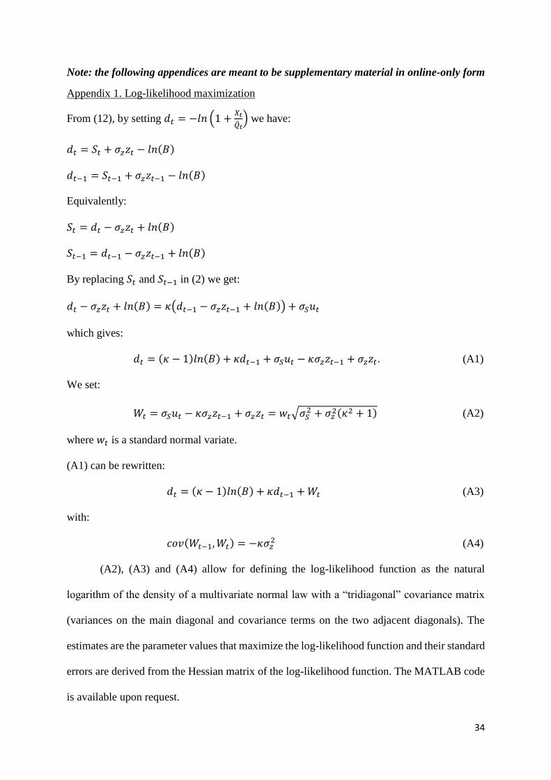
Appendix 1. Log-likelihood maximization

From (12), by setting 𝑑𝑡 = −𝑙𝑛 (1 +𝑋𝑡

�̃�𝑡) we have:

𝑑𝑡 = 𝑆𝑡 + 𝜎𝑧𝑧𝑡 − 𝑙𝑛(𝐵)

𝑑𝑡−1 = 𝑆𝑡−1 + 𝜎𝑧𝑧𝑡−1 − 𝑙𝑛(𝐵)

Equivalently:

𝑆𝑡 = 𝑑𝑡 − 𝜎𝑧𝑧𝑡 + 𝑙𝑛(𝐵)

𝑆𝑡−1 = 𝑑𝑡−1 − 𝜎𝑧𝑧𝑡−1 + 𝑙𝑛(𝐵)

By replacing 𝑆𝑡 and 𝑆𝑡−1 in (2) we get:

𝑑𝑡 − 𝜎𝑧𝑧𝑡 + 𝑙𝑛(𝐵) = 𝜅(𝑑𝑡−1 − 𝜎𝑧𝑧𝑡−1 + 𝑙𝑛(𝐵)) + 𝜎𝑆𝑢𝑡

which gives:

𝑑𝑡 = (𝜅 − 1)𝑙𝑛(𝐵) + 𝜅𝑑𝑡−1 + 𝜎𝑆𝑢𝑡 − 𝜅𝜎𝑧𝑧𝑡−1 + 𝜎𝑧𝑧𝑡. (A1)

We set:

𝑊𝑡 = 𝜎𝑆𝑢𝑡 − 𝜅𝜎𝑧𝑧𝑡−1 + 𝜎𝑧𝑧𝑡 = 𝑤𝑡√𝜎𝑆2 + 𝜎𝑧

2(𝜅2 + 1) (A2)

where 𝑤𝑡 is a standard normal variate.

(A1) can be rewritten:

𝑑𝑡 = (𝜅 − 1)𝑙𝑛(𝐵) + 𝜅𝑑𝑡−1 + 𝑊𝑡 (A3)

with:

𝑐𝑜𝑣(𝑊𝑡−1, 𝑊𝑡) = −𝜅𝜎𝑧2 (A4)

(A2), (A3) and (A4) allow for defining the log-likelihood function as the natural

logarithm of the density of a multivariate normal law with a “tridiagonal” covariance matrix

(variances on the main diagonal and covariance terms on the two adjacent diagonals). The

estimates are the parameter values that maximize the log-likelihood function and their standard

errors are derived from the Hessian matrix of the log-likelihood function. The MATLAB code

is available upon request.

35

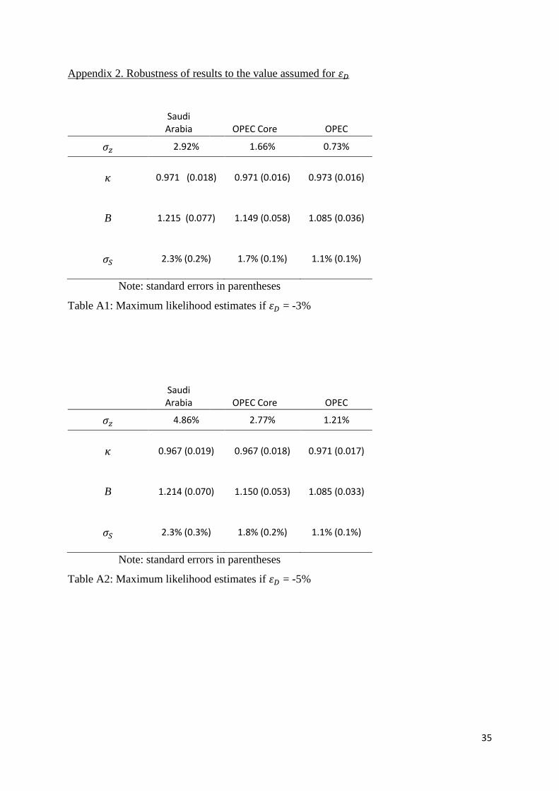
Appendix 2. Robustness of results to the value assumed for 𝜀𝐷

Saudi Arabia

OPEC Core

OPEC

𝜎𝑧 2.92% 1.66% 0.73%

𝜅 0.971 (0.018) 0.971 (0.016) 0.973 (0.016)

B 1.215 (0.077) 1.149 (0.058) 1.085 (0.036)

𝜎𝑆 2.3% (0.2%) 1.7% (0.1%) 1.1% (0.1%)

Note: standard errors in parentheses

Table A1: Maximum likelihood estimates if 𝜀𝐷 = -3%

Saudi Arabia

OPEC Core

OPEC

𝜎𝑧 4.86% 2.77% 1.21%

𝜅 0.967 (0.019) 0.967 (0.018) 0.971 (0.017)

B 1.214 (0.070) 1.150 (0.053) 1.085 (0.033)

𝜎𝑆 2.3% (0.3%) 1.8% (0.2%) 1.1% (0.1%)

Note: standard errors in parentheses

Table A2: Maximum likelihood estimates if 𝜀𝐷 = -5%

36

Saudi Arabia

OPEC Core

OPEC

𝜎𝑧 13.47% 8.01% 3.94%

𝜅 0.953 (0.027) 0.953 (0.023) 0.956 (0.021)

B 1.218 (0.055) 1.154 (0.041) 1.087 (0.026)

𝜎𝑆 2.4% (0.5%) 1.9% (0.3%) 1.2% (0.2%)

Note: standard errors in parentheses

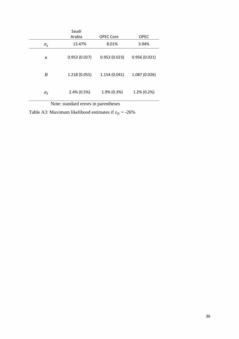
Table A3: Maximum likelihood estimates if 𝜀𝐷 = -26%

37

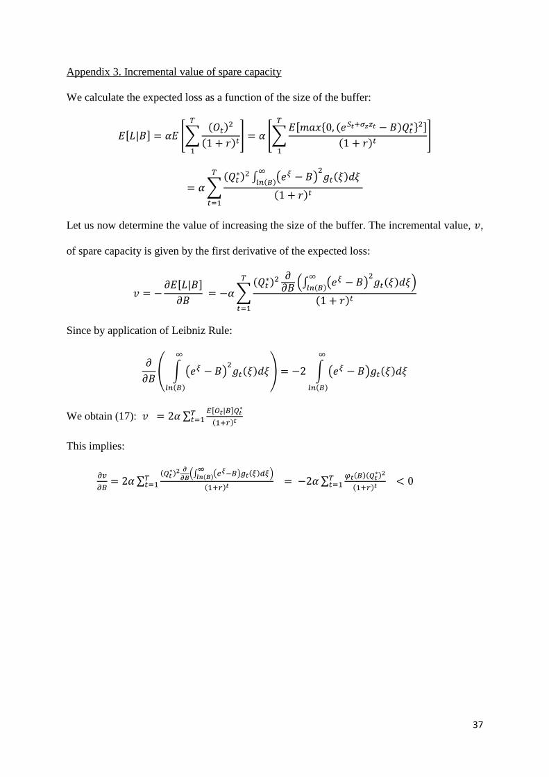
Appendix 3. Incremental value of spare capacity

We calculate the expected loss as a function of the size of the buffer:

𝐸[𝐿|𝐵] = 𝛼𝐸 [∑(𝑂𝑡)2

(1 + 𝑟)𝑡

𝑇

1

] = 𝛼 [∑𝐸[𝑚𝑎𝑥{0, (𝑒𝑆𝑡+𝜎𝑧𝑧𝑡 − 𝐵)𝑄𝑡

∗}2]

(1 + 𝑟)𝑡

𝑇

1

]

= 𝛼 ∑(𝑄𝑡

∗)2 ∫ (𝑒𝜉 − 𝐵)2

𝑔𝑡(𝜉)𝑑𝜉∞

𝑙𝑛(𝐵)

(1 + 𝑟)𝑡

𝑇

𝑡=1

Let us now determine the value of increasing the size of the buffer. The incremental value, 𝑣,

of spare capacity is given by the first derivative of the expected loss:

𝑣 = −𝜕𝐸[𝐿|𝐵]

𝜕𝐵 = −𝛼 ∑

(𝑄𝑡∗)2 𝜕

𝜕𝐵(∫ (𝑒𝜉 − 𝐵)

2𝑔𝑡(𝜉)𝑑𝜉

∞

𝑙𝑛(𝐵))

(1 + 𝑟)𝑡

𝑇

𝑡=1

Since by application of Leibniz Rule:

𝜕

𝜕𝐵( ∫ (𝑒𝜉 − 𝐵)

2𝑔𝑡(𝜉)𝑑𝜉

∞

𝑙𝑛(𝐵)

) = −2 ∫ (𝑒𝜉 − 𝐵)𝑔𝑡(𝜉)𝑑𝜉

∞

𝑙𝑛(𝐵)

We obtain (17): 𝑣 = 2𝛼 ∑𝐸[𝑂𝑡|𝐵]𝑄𝑡

∗

(1+𝑟)𝑡𝑇𝑡=1

This implies:

𝜕𝑣

𝜕𝐵= 2𝛼 ∑

(𝑄𝑡∗)2 𝜕

𝜕𝐵(∫ (𝑒𝜉−𝐵)𝑔𝑡(𝜉)𝑑𝜉

∞𝑙𝑛(𝐵) )

(1+𝑟)𝑡 = −2𝛼 ∑

𝜑𝑡(𝐵)(𝑄𝑡∗)2

(1+𝑟)𝑡𝑇𝑡=1 < 0𝑇

𝑡=1

38

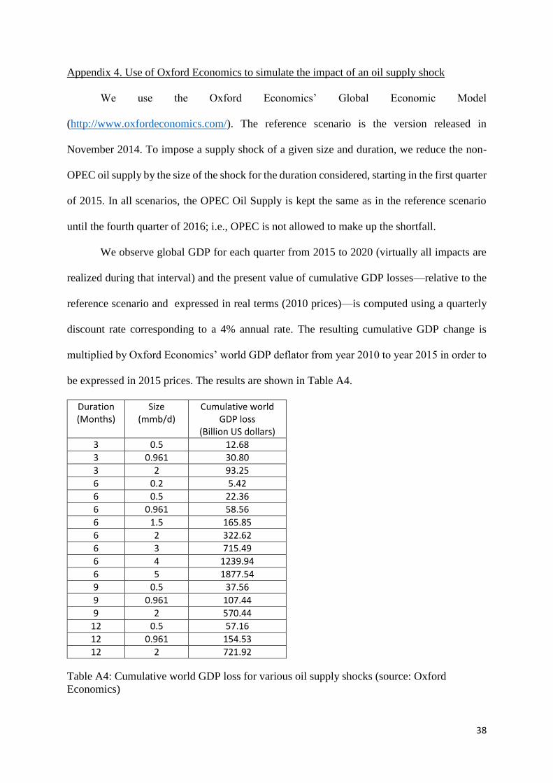
Appendix 4. Use of Oxford Economics to simulate the impact of an oil supply shock

We use the Oxford Economics’ Global Economic Model

(http://www.oxfordeconomics.com/). The reference scenario is the version released in

November 2014. To impose a supply shock of a given size and duration, we reduce the non-

OPEC oil supply by the size of the shock for the duration considered, starting in the first quarter

of 2015. In all scenarios, the OPEC Oil Supply is kept the same as in the reference scenario

until the fourth quarter of 2016; i.e., OPEC is not allowed to make up the shortfall.

We observe global GDP for each quarter from 2015 to 2020 (virtually all impacts are

realized during that interval) and the present value of cumulative GDP losses—relative to the

reference scenario and expressed in real terms (2010 prices)—is computed using a quarterly

discount rate corresponding to a 4% annual rate. The resulting cumulative GDP change is

multiplied by Oxford Economics’ world GDP deflator from year 2010 to year 2015 in order to

be expressed in 2015 prices. The results are shown in Table A4.

Duration (Months)

Size (mmb/d)

Cumulative world GDP loss

(Billion US dollars)

3 0.5 12.68

3 0.961 30.80

3 2 93.25

6 0.2 5.42

6 0.5 22.36

6 0.961 58.56

6 1.5 165.85

6 2 322.62

6 3 715.49

6 4 1239.94

6 5 1877.54

9 0.5 37.56

9 0.961 107.44

9 2 570.44

12 0.5 57.16

12 0.961 154.53

12 2 721.92

Table A4: Cumulative world GDP loss for various oil supply shocks (source: Oxford

Economics)