Advances in Engineering Software 40 (2009) 564–569

Contents lists available at ScienceDirect

Advances in Engineering Software

journal homepage: www.elsevier .com/locate /advengsoft

Open source BEM library

Paweł Wieleba *, Jan SikoraInstitute of Theory of Electrical Engineering, Measurement and Information Systems, Warsaw University of Technology, ul. Koszykowa 75, 00-662 Warszawa, Poland

a r t i c l e i n f o

Article history:Received 4 January 2008Received in revised form 30 April 2008Accepted 21 October 2008Available online 13 December 2008

Keywords:Boundary element methodOpen source BEM libraryDiffusion optical tomography

0965-9978/$ - see front matter � 2008 Elsevier Ltd. Adoi:10.1016/j.advengsoft.2008.10.007

* Corresponding author.E-mail address: p.wieleba@iem.pw.edu.pl (P. Wiel

a b s t r a c t

This article presents the project of the new open source boundary element method library. It discussesmain goals of the project and its characteristics consistent with the ‘good open source project’. It coverslicense conditions, chosen technology, design of the project as well as development process.

� 2008 Elsevier Ltd. All rights reserved.

1. Introduction 2. BEM and diffusion optical tomography

For a few decades rapid development of boundary elementmethod (BEM) can be observed [1–8]. During that time range ofBEM’s application has increased [9–12]. Among other things it isused in electromagnetic, thermal or optical analysis. However itis not easy to find ready to use BEM implementations. The situationbecomes more difficult if it has been tried to find the free opensource software. It is even worse if specialised BEM software appli-cable for example to diffusion optical tomography is needed. Oneof the reasons why this state is maintained, might be the complex-ity of integration (in particular singular integrals) which has to bedone in BEM calculations. However, this is not a problem whichcannot be overcome [13]. The need for the BEM calculations soft-ware exists and is unquestionable, but it has been only insignifi-cantly implemented (Table A.1). It appears that industrial andscientific groups would like to have a well designed platform forBEM calculations. It should be universal but at the same time itsmodularity should easily enable application in very specific tasks.If needed, writing own plugins/modules, extending its functional-ity of solving other boundary integral equations (BIE), usage ofother for example integration algorithms or set of linear equationssolvers, must be simple. Moreover ability of using only selected,single modules in external projects is expected. The needs andexpectations mentioned above caused that the platform for BEMcalculations is being realised. Particular elements of the projectare introduced in the following sections.

ll rights reserved.

eba).

Before beginning work on the project’s model, the method andits example application has to be introduced. Here boundary ele-ment method in diffusion optical tomography (DOT) will be used.Why DOT? There are plenty of excellent papers in which imple-mentation of finite element method is presented (see for examplethe works of Prof. Arridge [14,15]). However only the BEM offered avery simple and effective from patient to patient creation of thegood quality surface meshes of the heads’ layers — also taking intoaccount the cerebrospinal fluid (CSF) layer [16]. Especially in threedimensions, generation of the good quality surface meshes is mucheasier and more effective in BEM than in FEM [17]. Descriptionhere will be limited only to general concepts important to themodel and its implementation.

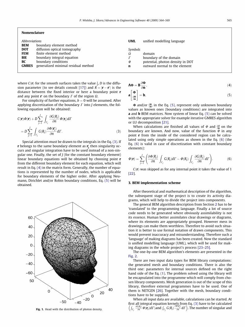
The main purpose of the library is the ability of doing all essen-tial calculations to solve the specific problem. Visualization of thesolution, using input mesh and output data, can be done usingeg. MATLAB. Fig. 1 presents baby’s head with the distribution ofphoton density calculated by this library.

Main interest will be devoted to the diffusion equation as it isthe approximation used in DOT [12,18–20]. The following equationpresents its differential form:

r2UðrÞ � k2UðrÞ ¼ b; ð1Þwhere the potential function U represents the photon density, k isthe wave number and b represents internal sources.

As BEM uses boundary integral equations (BIE) the integralform of Eq. (1) is:

CðrÞUðrÞ þ DZ

C

@GðRÞ@n

Uðr0ÞdCðr0Þ

¼ DZ

CGðRÞ @Uðr

0Þ@n

dCðr0Þ þZ Z

XGðRÞbdXðr0Þ; ð2Þ

Nomenclature

AbbreviationsBEM boundary element methodDOT diffusion optical tomographyFEM finite element methodBIE boundary integral equationBC boundary conditionsGMRES generalized minimal residual method

UML unified modelling language

SymbolsX domainC boundary of the domainU potential, photon density in DOTn outward normal to the element

P. Wieleba, J. Sikora / Advances in Engineering Software 40 (2009) 564–569 565

where CðrÞ for the smooth surfaces takes the value 12, D is the diffu-

sion parameter (to see details consult [17]) and R ¼ jr� r0j is thedistance between the fixed interior or here a boundary point rand any point r0 on the boundary C of the region X.

For simplicity of further equations, b ¼ 0 will be assumed. Afterapplying discretization of the boundary C into J elements, the fol-lowing equation will be obtained:

CðrÞUðrÞ þ DXJ

j¼1

ZCj

@GðRjÞ@n

UðrjÞdC

¼ DXJ

j¼1

ZCj

GðRjÞ@Uðr0jÞ@n

dC: ð3Þ

Special attention must be drawn to the integrals in the Eq. (3). Ifr belongs to the same boundary element as r0j then singularity oc-curs and singular integration have to be used instead of a non-sin-gular one. Finally, the set of J (for the constant boundary element)linear boundary equations will be obtained by choosing point rfrom the different boundary element for each equation, which willresult in Eq. (4) in the matrix form. Generally, the number of equa-tions is represented by the number of nodes, which is applicablefor boundary elements of the higher order. After applying Neu-mann, Dirichlet and/or Robin boundary conditions, Eq. (5) will beobtained.

Fig. 1. Head with the distribution of photon density.

AU ¼ B@U@n

; ð4Þ

aU@U@n

" #¼ b; ð5Þ

U and/or @U@n, in the Eq. (5), represent only unknown boundary

values as known ones (boundary conditions) are integrated intoa and b BEM matrices. Now system of linear Eq. (5) can be solvedwith the appropriate solver for example iterative GMRES algorithmor LU decomposition [21].

When calculations are finished all values of U and @U@n on the

boundary are known. And now, value of the function U in anypoint r from the inside of the considered region can be calcu-lated using only simple operations as shown in the Eq. (6) (theEq. (6) is valid in case of discretization with constant boundaryelements):

UðrÞ ¼XJ

j¼1

@UðRjÞ@n

ZCj

GðRjÞdC�UðRjÞZ

Cj

@GðRjÞ@n

dC

!: ð6Þ

CðrÞ was skipped as for any internal point it takes the value of 1[22].

3. BEM implementation scheme

After theoretical and mathematical description of the algorithm,the subsequent stage of the project is to create its activity dia-grams, which will help to divide the project into components.

The general BEM algorithm description from Section 2 has to be‘translated’ to the programming language. Finally a lot of sourcecode needs to be generated where obviously assimilability is notits essence. Human better assimilates clear drawings or diagrams,where its elements are appropriately grouped. However mess indrawings can make them worthless. Therefore to avoid such situa-tion it is better to use formal notation of drawn components. Thiswould prevent inaccuracy and misunderstanding. Therefore such a‘language’ of making diagrams has been created. Now the standardis unified modelling language (UML), which will be used for mak-ing diagrams in the whole project’s process [23–25].

The one-by-one BEM algorithm’s elements are presented in theFig. 2.

There are two input data types for BEM library computations:the generated mesh and boundary conditions. There is also thethird one: parameters for internal sources defined on the righthand side of the Eq. (1). The problem solved using the library willbe encapsulated into the programme which will comply from cho-sen library components. Mesh generation is out of the scope of thislibrary, therefore external programmes have to be used. One ofthem is NETGEN [26]. Together with the mesh, boundary condi-tions have to be supplied.

When all input data are available, calculations can be started. Atfirst all integral equation kernels from Eq. (3) have to be calculatedR

Cj

@GðRjÞ@n UðrjÞdCÞand

RCj

GðRjÞ@Uðr0

jÞ

@n dC� �

. The number of singular and

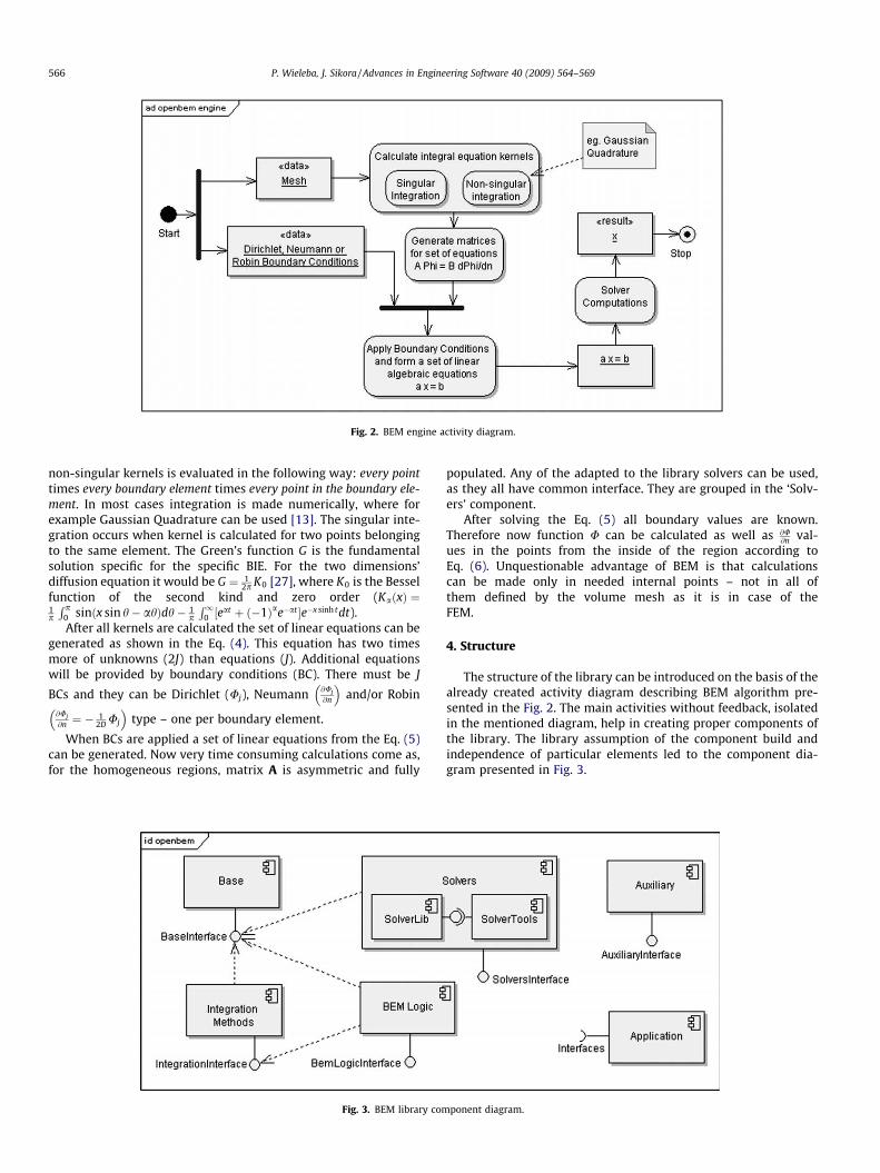
Fig. 2. BEM engine activity diagram.

566 P. Wieleba, J. Sikora / Advances in Engineering Software 40 (2009) 564–569

non-singular kernels is evaluated in the following way: every pointtimes every boundary element times every point in the boundary ele-ment. In most cases integration is made numerically, where forexample Gaussian Quadrature can be used [13]. The singular inte-gration occurs when kernel is calculated for two points belongingto the same element. The Green’s function G is the fundamentalsolution specific for the specific BIE. For the two dimensions’diffusion equation it would be G ¼ 1

2p K0 [27], where K0 is the Besselfunction of the second kind and zero order (KaðxÞ ¼1p

R p0 sinðx sin h� ahÞdh� 1

p

R10 ½eat þ ð�1Þae�at �e�x sinh tdt).

After all kernels are calculated the set of linear equations can begenerated as shown in the Eq. (4). This equation has two timesmore of unknowns (2J) than equations (J). Additional equationswill be provided by boundary conditions (BC). There must be J

BCs and they can be Dirichlet (Uj), Neumann @Uj

@n

� �and/or Robin

@Uj

@n ¼ � 12D Uj

� �type – one per boundary element.

When BCs are applied a set of linear equations from the Eq. (5)can be generated. Now very time consuming calculations come as,for the homogeneous regions, matrix A is asymmetric and fully

Fig. 3. BEM library com

populated. Any of the adapted to the library solvers can be used,as they all have common interface. They are grouped in the ‘Solv-ers’ component.

After solving the Eq. (5) all boundary values are known.Therefore now function U can be calculated as well as @U

@n val-ues in the points from the inside of the region according toEq. (6). Unquestionable advantage of BEM is that calculationscan be made only in needed internal points – not in all ofthem defined by the volume mesh as it is in case of theFEM.

4. Structure

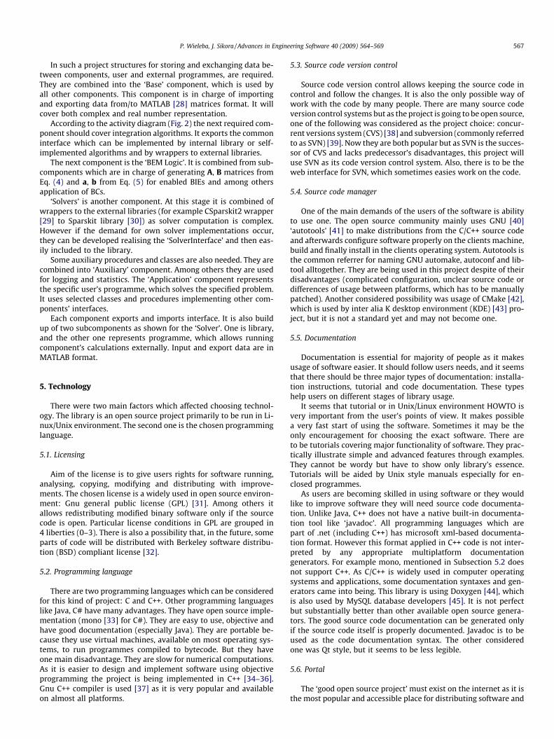
The structure of the library can be introduced on the basis of thealready created activity diagram describing BEM algorithm pre-sented in the Fig. 2. The main activities without feedback, isolatedin the mentioned diagram, help in creating proper components ofthe library. The library assumption of the component build andindependence of particular elements led to the component dia-gram presented in Fig. 3.

ponent diagram.

P. Wieleba, J. Sikora / Advances in Engineering Software 40 (2009) 564–569 567

In such a project structures for storing and exchanging data be-tween components, user and external programmes, are required.They are combined into the ‘Base’ component, which is used byall other components. This component is in charge of importingand exporting data from/to MATLAB [28] matrices format. It willcover both complex and real number representation.

According to the activity diagram (Fig. 2) the next required com-ponent should cover integration algorithms. It exports the commoninterface which can be implemented by internal library or self-implemented algorithms and by wrappers to external libraries.

The next component is the ‘BEM Logic’. It is combined from sub-components which are in charge of generating A, B matrices fromEq. (4) and a, b from Eq. (5) for enabled BIEs and among othersapplication of BCs.

‘Solvers’ is another component. At this stage it is combined ofwrappers to the external libraries (for example CSparskit2 wrapper[29] to Sparskit library [30]) as solver computation is complex.However if the demand for own solver implementations occur,they can be developed realising the ‘SolverInterface’ and then eas-ily included to the library.

Some auxiliary procedures and classes are also needed. They arecombined into ‘Auxiliary’ component. Among others they are usedfor logging and statistics. The ‘Application’ component representsthe specific user’s programme, which solves the specified problem.It uses selected classes and procedures implementing other com-ponents’ interfaces.

Each component exports and imports interface. It is also buildup of two subcomponents as shown for the ‘Solver’. One is library,and the other one represents programme, which allows runningcomponent’s calculations externally. Input and export data are inMATLAB format.

5. Technology

There were two main factors which affected choosing technol-ogy. The library is an open source project primarily to be run in Li-nux/Unix environment. The second one is the chosen programminglanguage.

5.1. Licensing

Aim of the license is to give users rights for software running,analysing, copying, modifying and distributing with improve-ments. The chosen license is a widely used in open source environ-ment: Gnu general public license (GPL) [31]. Among others itallows redistributing modified binary software only if the sourcecode is open. Particular license conditions in GPL are grouped in4 liberties (0–3). There is also a possibility that, in the future, someparts of code will be distributed with Berkeley software distribu-tion (BSD) compliant license [32].

5.2. Programming language

There are two programming languages which can be consideredfor this kind of project: C and C++. Other programming languageslike Java, C# have many advantages. They have open source imple-mentation (mono [33] for C#). They are easy to use, objective andhave good documentation (especially Java). They are portable be-cause they use virtual machines, available on most operating sys-tems, to run programmes compiled to bytecode. But they haveone main disadvantage. They are slow for numerical computations.As it is easier to design and implement software using objectiveprogramming the project is being implemented in C++ [34–36].Gnu C++ compiler is used [37] as it is very popular and availableon almost all platforms.

5.3. Source code version control

Source code version control allows keeping the source code incontrol and follow the changes. It is also the only possible way ofwork with the code by many people. There are many source codeversion control systems but as the project is going to be open source,one of the following was considered as the project choice: concur-rent versions system (CVS) [38] and subversion (commonly referredto as SVN) [39]. Now they are both popular but as SVN is the succes-sor of CVS and lacks predecessor’s disadvantages, this project willuse SVN as its code version control system. Also, there is to be theweb interface for SVN, which sometimes easies work on the code.

5.4. Source code manager

One of the main demands of the users of the software is abilityto use one. The open source community mainly uses GNU [40]‘autotools’ [41] to make distributions from the C/C++ source codeand afterwards configure software properly on the clients machine,build and finally install in the clients operating system. Autotools isthe common referrer for naming GNU automake, autoconf and lib-tool alltogether. They are being used in this project despite of theirdisadvantages (complicated configuration, unclear source code ordifferences of usage between platforms, which has to be manuallypatched). Another considered possibility was usage of CMake [42],which is used by inter alia K desktop environment (KDE) [43] pro-ject, but it is not a standard yet and may not become one.

5.5. Documentation

Documentation is essential for majority of people as it makesusage of software easier. It should follow users needs, and it seemsthat there should be three major types of documentation: installa-tion instructions, tutorial and code documentation. These typeshelp users on different stages of library usage.

It seems that tutorial or in Unix/Linux environment HOWTO isvery important from the user’s points of view. It makes possiblea very fast start of using the software. Sometimes it may be theonly encouragement for choosing the exact software. There areto be tutorials covering major functionality of software. They prac-tically illustrate simple and advanced features through examples.They cannot be wordy but have to show only library’s essence.Tutorials will be aided by Unix style manuals especially for en-closed programmes.

As users are becoming skilled in using software or they wouldlike to improve software they will need source code documenta-tion. Unlike Java, C++ does not have a native built-in documenta-tion tool like ‘javadoc’. All programming languages which arepart of .net (including C++) has microsoft xml-based documenta-tion format. However this format applied in C++ code is not inter-preted by any appropriate multiplatform documentationgenerators. For example mono, mentioned in Subsection 5.2 doesnot support C++. As C/C++ is widely used in computer operatingsystems and applications, some documentation syntaxes and gen-erators came into being. This library is using Doxygen [44], whichis also used by MySQL database developers [45]. It is not perfectbut substantially better than other available open source genera-tors. The good source code documentation can be generated onlyif the source code itself is properly documented. Javadoc is to beused as the code documentation syntax. The other consideredone was Qt style, but it seems to be less legible.

5.6. Portal

The ‘good open source project’ must exist on the internet as it isthe most popular and accessible place for distributing software and

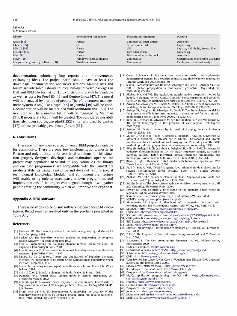
Table A.1BEM library review.

Library Environment (language) Distribution conditions Purpose

ABEM [54] Fortran Commercial, open source AcousticsLibBem [55] C++ Semi commercial Laplace eq.BEMLIB [56] Fortran GPL Laplace, Helmholtz, Stokes flowBIEPACK [57] Fortran Free open source Laplace eq.BEA [58] Fortran Distributed with the book AcousticsBEASY [59] Windows or Unix binaries Commercial Construction engineering, acousticsIntegrated engineering software [60] Windows binaries Commercial Fields, wave, thermal analysis

568 P. Wieleba, J. Sikora / Advances in Engineering Software 40 (2009) 564–569

documentation, submitting bug reports and improvements,exchanging ideas. The project portal should have at least thedownloads, documentation and news sections. Mailing lists andforum are advisable. Library sources, binary software packages inDEB and RPM file format for Linux distributions will be availableas well as ports for FreeBSD [46] and Gentoo Linux [47]. The portalwill be managed by a group of people. Therefore content manage-ment system (CMS) like Drupal [48] or Joomla [49] will be used.Documentation will be maintained with MoinMoin wiki [50]. Thenext step will be a mailing list. It will be managed by Mailman[51]. If necessary a forum will be created. The considered possibil-ities, also open source, are phpBB [52] (inter alia used by gentoo[47]) or less probably, Java based jforum [53].

6. Conclusions

There are not any open source, universal BEM projects availablefor community. There are only few implementations, mostly inFortran and only applicable for restricted problems. In this situa-tion properly designed, developed and maintained open sourceproject may popularise BEM and its application. As the libraryand enclosed programmes’ are compatible with the Linux/Unixproducts style, its usage is intuitive and does not require specialtechnological knowledge. Modular and component architecturewill enable using only selected parts in own programmes andimplementations. If the project will be good enough, it will gatherpeople creating the community, which will improve and expand it.

Appendix A. BEM software

There is no wide choice of any software destined for BEM calcu-lations. Broad searches resulted only in the products presented inTable A.1.

References

[1] Banerjee PK. The boundary element methods in engineering. McGraw-HillBook Company; 1994.

[2] Becker AA. The boundary element method in engineering. A completecourse. McGraw-Hill Book Company; 1992.

[3] Beer G. Programming the boundary element method. An introduction forengineers. John Wiley & Sons; 2001.

[4] Beer G, Watson JO. Introduction to finite and boundary element methods forengineers. John Wiley & Sons; 1992.

[5] Tanaka M, Du Q, editors. Theory and applications of boundary elementsmethods. In: Proceedings of 1st Japan–China symposium on boundary elementmethods, Pergamon, 1987.

[6] Bonnet M. Boundary integral equation methods for solid and fluids. John Wiley& Sons; 1995.

[7] Chen G, Zhou J. Boundary element methods. Academic Press; 1992.[8] Duddeck FME. Fourier BEM. Lecture notes in applied mechanics, vol.

5. Springer-Verlag; 2002.[9] Amaratunga K. A wavelet-based approach for compressing kernel data in

large-scale simulations of 3D integral problems. Comput Sci Eng 2000:34–45.July/August.

[10] Frijns JHM, de Snoo SL, Schoonhoven R. Improving the accuracy of theboundary element method by the use of second-order interpolation functions.IEEE Trans Biomed Eng 2000;47(10):1336–46.

[11] Guven I, Madenci E. Transient heat conducting analysis in a piecewisehomogeneous domain by a coupled boundary and finite element method. IntJ Numer Meth Eng 2003;56:351–80.

[12] Sikora J, Zacharopoulos AD, Douiri A, Schweiger M, Horesh L, Arridge SR, et al.Diffuse photon propagation in multilayered geometries. Phys Med Biol2006;51(3):97–516.

[13] Aliabadi MH, Hall WS. The regularizing transformation integration method forboundary element kernels. Comparison with series expansion and weightedGaussian integration methods. Eng Anal Bound Elements 1989;6(2):66–70.

[14] Arridge SR, Schweiger M, Hiraoka M, Delpy DT. A finite element approach formodeling photon transport in tissue. Med Phys 1993;20(2):299–309.

[15] Arridge SR, Dehghani H, Schweiger M, Okada E. The finite element model forthe propagation of light in scaterring media: a direct method for domains withnonscattering regions. Med Phys 2000;27(1):252–64.

[16] Riley JD, Dehghani H, Schweiger M, Arridge SR, Ripoll J, Nieto-Vesperinas M.3D optical tomography in the presence of void regions. Opt Express2000;7(13).

[17] Arridge SR. Optical tomography in medical imaging. Inverse Problems1999;15(2):R41–93.

[18] Muller G, Chance B, Alfano R, Arridge S, Beuthan J, Gratton E, Kaschke M,Masters B, Svanberg S, van der Zee P, editors. The forward and inverseproblems in time-resolved infrared imaging. In: Proceedings of the SPIE,medical optical tomography: functional imaging and monitoring, 1993.

[19] Riley JD, Arridge SR, Chrysanthou Y, Dehghani H, Hillman EMC, Schweiger M.Radiosity diffusion model in 3D. In: Stefan Andersson-Engels, Michael F.Kaschke, editors. Photon migration, optical coherence tomography, andmicroscopy. Proceedings of SPIE, vols. 18–21. June 2001. p. 153–64.

[20] Ripoll J. Light diffusion in turbid media with biomedical application. PhDThesis, University of Madrid, 2000.

[21] Saad Y, Schultz MH. GMRES: a generalized minimal residual algorithm forsolving nonsymmetric linear systems. SIAM J Sci Statist Comput1986;7(3):856–69. April.

[22] Aliabadi MH. The boundary element method. Applications in solids andstructures, vol. 2. John Wiley & Sons, LTD; 2002.

[23] Ambler Scott W. The object primer agile model-driven development with UML2.0.. Cambridge University Press; 2004.

[24] Fowler M. UML distilled: a brief guide to the standard object modelinglanguage. 3rd ed. Addison-Wesley; 2003.

[25] Sommerville I. Software engineering. 7th ed. Addison-Wesley; 2004.[26] NETGEN. <http://www.hpfem.jku.at/netgen/>.[27] Abramowitz M, Stegun IA. Handbook of mathematical functions with

formulas, graphs and mathematical tables. John Wiley, New York, 1973.[28] MATLAB. <http://www.mathworks.com/products/matlab/>.[29] CSparskit2. <http://bemlab.org/csparskit2/>.[30] Sparskit. <http://www-users.cs.umn.edu/saad/software/SPARSKIT/sparskit.html>.[31] GNU public license. <http://www.gnu.org/copyleft/gpl.html>.[32] BSD license. <http://www.opensource.org/licenses/bsd-license.html>.[33] Mono. <http://www.mono-project.com/>.[34] Eckel B. Thinking in C++, Introduction to standard C++. 2nd ed., vol. 1. Prentice-

Hall, 2000.[35] Eckel B. Thinking in C++. Practical programming, second ed., vol. 2. Prentice-

Hall; 2003.[36] Stroustrup B. The C++ programming language. 3rd ed. Addison-Wesley

Professional; 2000.[37] GNU C++ compiler. <http://gcc.gnu.org/>.[38] Concurrent versions system (CVS). <http://www.nongnu.org/cvs/>.[39] Subversion (SVN). <http://subversion.tigris.org/>.[40] GNU. <http://www.gnu.org/>.[41] Tom Tromey Ian Lance Taylor Gary V. Vaughan, Ben Elliston. GNU autoconf,

automake, and libtool. Sams, 2000.[42] Cmake (cross-platform make). <http://www.cmake.org/>.[43] K desktop environment (kde). <http://www.kde.org/>.[44] Doxygen. <http://www.stack.nl/dimitri/doxygen/>.[45] MySQL application programming interface (API). <http://dev.mysql.com/

sources/doxygen/mysql-5.1/>.[46] FreeBSD. <http://www.freebsd.org/>.[47] Gentoo linux. <http://www.gentoo.org/>.[48] Drupal cms. <http://www.drupal.org/>.[49] Joomla cms. <http://www.joomla.org/>.[50] Moinmoin wiki engine. <http://moinmoin.wikiwikiweb.de/>.[51] Mailman. <http://www.gnu.org/software/mailman/>.

P. Wieleba, J. Sikora / Advances in Engineering Software 40 (2009) 564–569 569

[52] phpBB. <http://www.phpbb.com/>.[53] Jforum. <http://www.jforum.net/>.[54] Abem. <http://www.boundary-element-method.com/>.[55] Libbem. <http://www.mis.mpg.de/scicomp/software/libbem/libbem.html>.[56] Bemlib. <http://dehesa.freeshell.org/BEMLIB/bemlib.shtml>.[57] Biepack. <http://www.math.uiowa.edu/atkinson/bie.html>.

[58] Wu TW. Boundary element acoustics: fundamentals and computercodes. WitPress; 2000.

[59] Beasy. <http://www.beasy.com/>.[60] Integrated engineering software. <http://www.integratedsoft.com/bem.

asp>.