open3dtools tutorial - open3dqsar -...
TRANSCRIPT
Open3DTOOLS
tutorial Starting Open3DALIGN
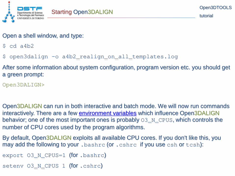
Open a shell window, and type:
$ cd a4b2
$ open3dalign -o a4b2_realign_on_all_templates.log
After some information about system configuration, program version etc. you should get a green prompt:
Open3DALIGN>
Open3DALIGN can run in both interactive and batch mode. We will now run commands interactively. There are a few environment variables which influence Open3DALIGN behavior; one of the most important ones is probably O3_N_CPUS, which controls the number of CPU cores used by the program algorithms.
By default, Open3DALIGN exploits all available CPU cores. If you don't like this, you may add the following to your .bashrc (or .cshrc if you use csh or tcsh):
export O3_N_CPUS=1 (for .bashrc)
setenv O3_N_CPUS 1 (for .cshrc)
Open3DTOOLS
tutorial Setting the number of CPU cores
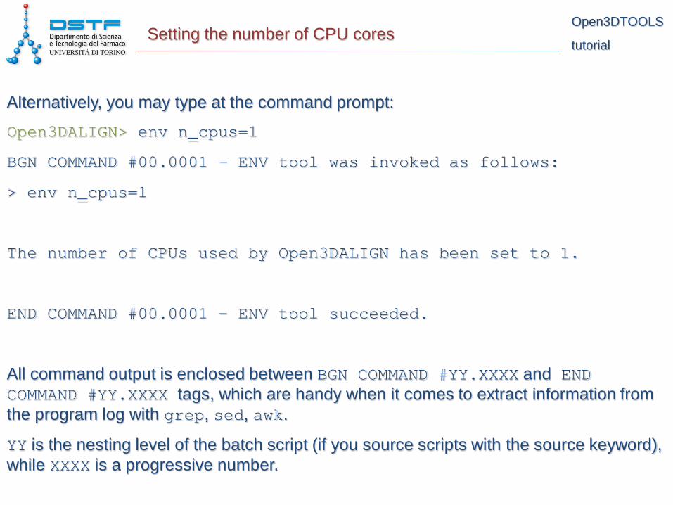
Alternatively, you may type at the command prompt:
Open3DALIGN> env n_cpus=1
BGN COMMAND #00.0001 - ENV tool was invoked as follows:
> env n_cpus=1
The number of CPUs used by Open3DALIGN has been set to 1.
END COMMAND #00.0001 - ENV tool succeeded.
All command output is enclosed between BGN COMMAND #YY.XXXX and END COMMAND #YY.XXXX tags, which are handy when it comes to extract information from the program log with grep, sed, awk.
YY is the nesting level of the batch script (if you source scripts with the source keyword), while XXXX is a progressive number.
Open3DTOOLS
tutorial Importing a SDF dataset
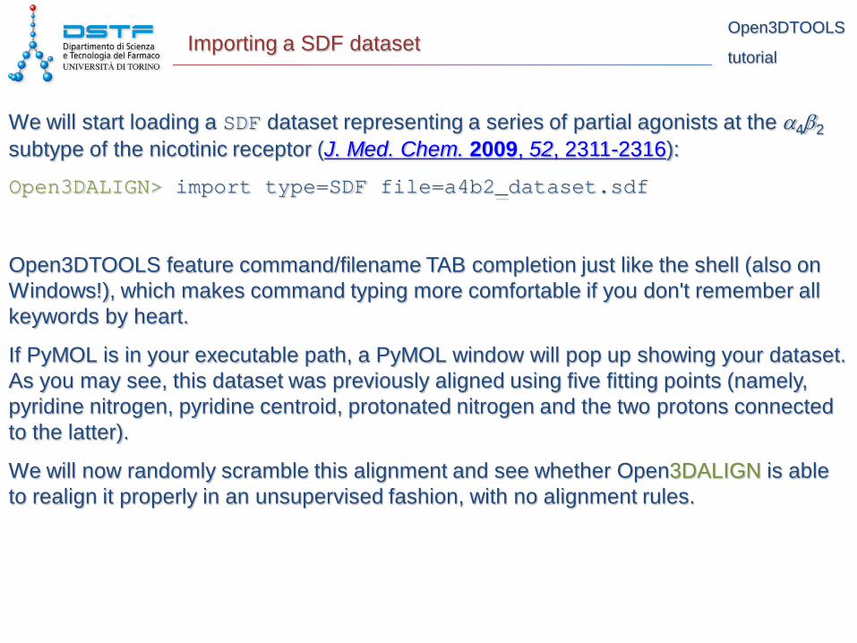
We will start loading a SDF dataset representing a series of partial agonists at the α4β2 subtype of the nicotinic receptor (J. Med. Chem. 2009, 52, 2311-2316):
Open3DALIGN> import type=SDF file=a4b2_dataset.sdf
Open3DTOOLS feature command/filename TAB completion just like the shell (also on Windows!), which makes command typing more comfortable if you don't remember all keywords by heart.
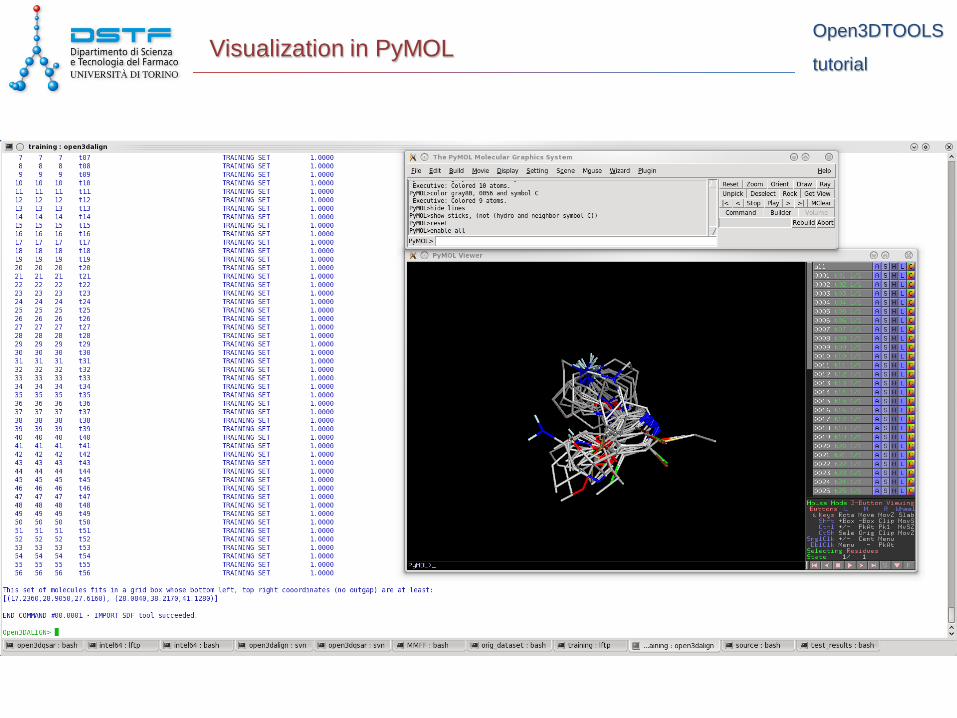
If PyMOL is in your executable path, a PyMOL window will pop up showing your dataset. As you may see, this dataset was previously aligned using five fitting points (namely, pyridine nitrogen, pyridine centroid, protonated nitrogen and the two protons connected to the latter).
We will now randomly scramble this alignment and see whether Open3DALIGN is able to realign it properly in an unsupervised fashion, with no alignment rules.
Open3DTOOLS
tutorial Visualization in PyMOL
Open3DTOOLS
tutorial Random scrambling of a SDF dataset
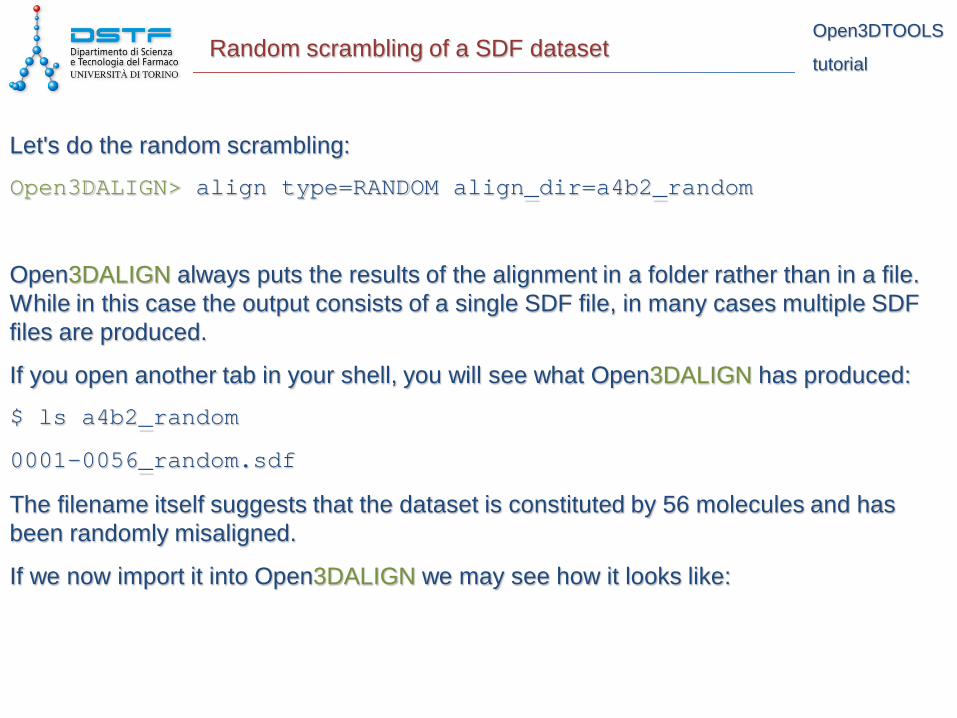
Let's do the random scrambling:
Open3DALIGN> align type=RANDOM align_dir=a4b2_random
Open3DALIGN always puts the results of the alignment in a folder rather than in a file. While in this case the output consists of a single SDF file, in many cases multiple SDF files are produced.
If you open another tab in your shell, you will see what Open3DALIGN has produced:
$ ls a4b2_random
0001-0056_random.sdf
The filename itself suggests that the dataset is constituted by 56 molecules and has been randomly misaligned.
If we now import it into Open3DALIGN we may see how it looks like:

Open3DTOOLS
tutorial Random scrambling of a SDF dataset
Open3DALIGN> import type=SDF file=a4b2_random/0001-0056_random.sdf
Open3DTOOLS
tutorial Realignment of a rigid dataset
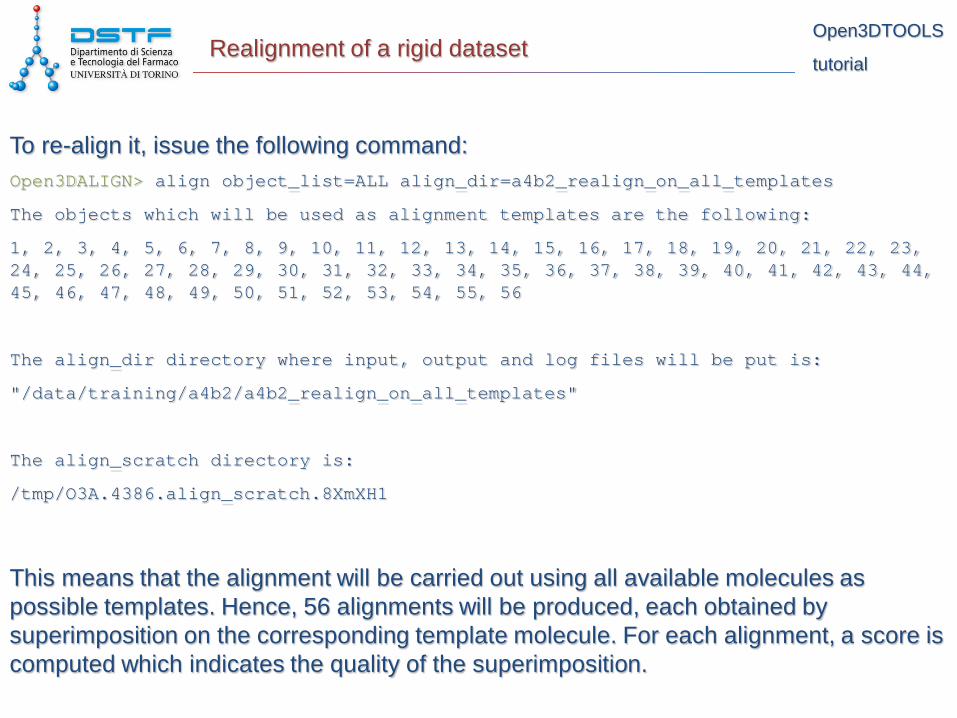
To re-align it, issue the following command: Open3DALIGN> align object_list=ALL align_dir=a4b2_realign_on_all_templates
The objects which will be used as alignment templates are the following:
1, 2, 3, 4, 5, 6, 7, 8, 9, 10, 11, 12, 13, 14, 15, 16, 17, 18, 19, 20, 21, 22, 23, 24, 25, 26, 27, 28, 29, 30, 31, 32, 33, 34, 35, 36, 37, 38, 39, 40, 41, 42, 43, 44, 45, 46, 47, 48, 49, 50, 51, 52, 53, 54, 55, 56
The align_dir directory where input, output and log files will be put is:
"/data/training/a4b2/a4b2_realign_on_all_templates"
The align_scratch directory is:
/tmp/O3A.4386.align_scratch.8XmXH1
This means that the alignment will be carried out using all available molecules as possible templates. Hence, 56 alignments will be produced, each obtained by superimposition on the corresponding template molecule. For each alignment, a score is computed which indicates the quality of the superimposition.
Open3DTOOLS
tutorial Alignment scores
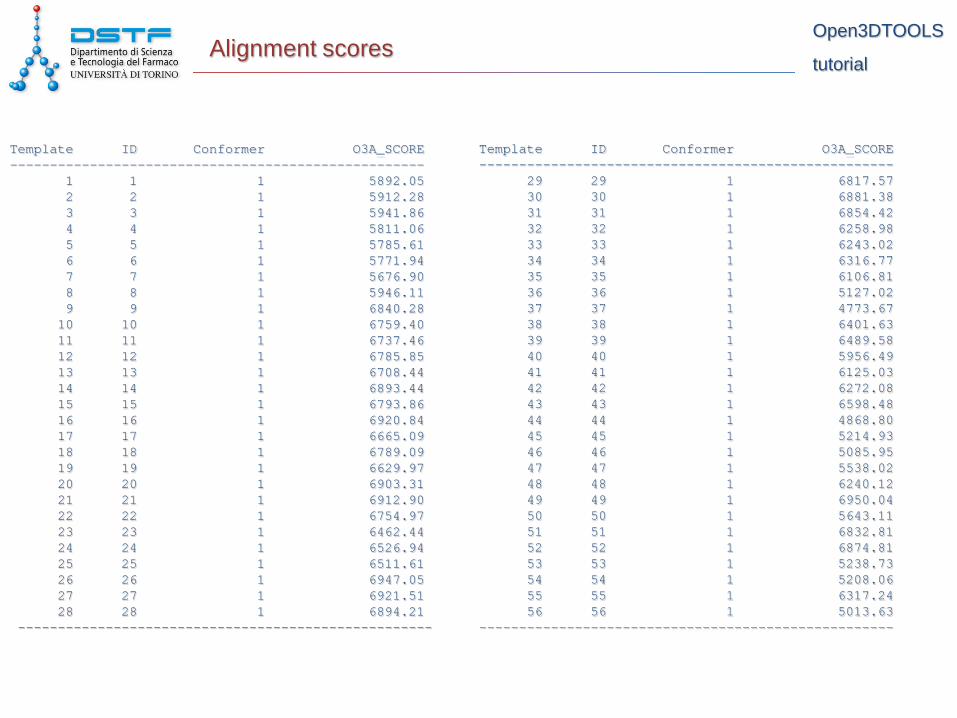
Template ID Conformer O3A_SCORE ---------------------------------------------------- 1 1 1 5892.05 2 2 1 5912.28 3 3 1 5941.86 4 4 1 5811.06 5 5 1 5785.61 6 6 1 5771.94 7 7 1 5676.90 8 8 1 5946.11 9 9 1 6840.28 10 10 1 6759.40 11 11 1 6737.46 12 12 1 6785.85 13 13 1 6708.44 14 14 1 6893.44 15 15 1 6793.86 16 16 1 6920.84 17 17 1 6665.09 18 18 1 6789.09 19 19 1 6629.97 20 20 1 6903.31 21 21 1 6912.90 22 22 1 6754.97 23 23 1 6462.44 24 24 1 6526.94 25 25 1 6511.61 26 26 1 6947.05 27 27 1 6921.51 28 28 1 6894.21 ----------------------------------------------------
Template ID Conformer O3A_SCORE ---------------------------------------------------- 29 29 1 6817.57 30 30 1 6881.38 31 31 1 6854.42 32 32 1 6258.98 33 33 1 6243.02 34 34 1 6316.77 35 35 1 6106.81 36 36 1 5127.02 37 37 1 4773.67 38 38 1 6401.63 39 39 1 6489.58 40 40 1 5956.49 41 41 1 6125.03 42 42 1 6272.08 43 43 1 6598.48 44 44 1 4868.80 45 45 1 5214.93 46 46 1 5085.95 47 47 1 5538.02 48 48 1 6240.12 49 49 1 6950.04 50 50 1 5643.11 51 51 1 6832.81 52 52 1 6874.81 53 53 1 5238.73 54 54 1 5208.06 55 55 1 6317.24 56 56 1 5013.63 ----------------------------------------------------
Open3DTOOLS
tutorial Find the best scoring alignment
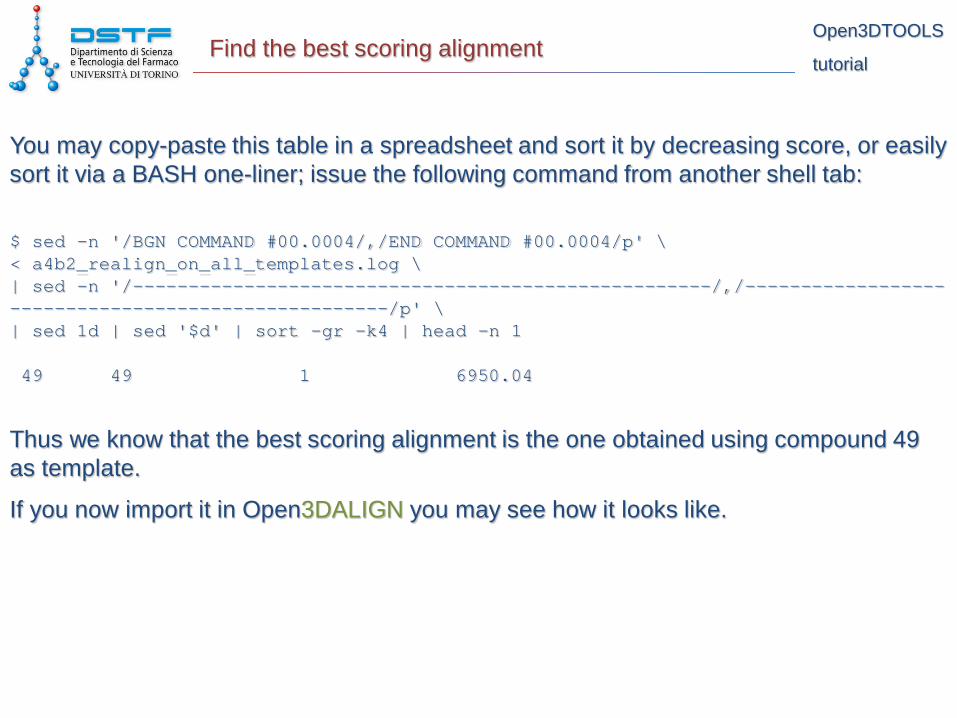
You may copy-paste this table in a spreadsheet and sort it by decreasing score, or easily sort it via a BASH one-liner; issue the following command from another shell tab:
$ sed -n '/BGN COMMAND #00.0004/,/END COMMAND #00.0004/p' \ < a4b2_realign_on_all_templates.log \ | sed -n '/----------------------------------------------------/,/----------------------------------------------------/p' \ | sed 1d | sed '$d' | sort -gr -k4 | head -n 1 49 49 1 6950.04
Thus we know that the best scoring alignment is the one obtained using compound 49 as template.
If you now import it in Open3DALIGN you may see how it looks like.
Open3DTOOLS
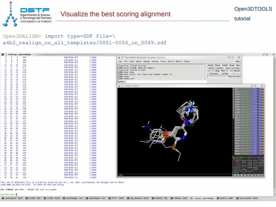
tutorial Visualize the best scoring alignment
Open3DALIGN> import type=SDF file=\ a4b2_realign_on_all_templates/0001-0056_on_0049.sdf

Open3DTOOLS
tutorial Import the aligned dataset in Open3DQSAR
Now you may exit Open3DALIGN:
Open3DALIGN> exit
Since Open3DALIGN strips properties from the aligned SDF, you may wish to restore them with a small script; alternatively you may conveniently import biological activities from a text file.
$ ../sh/copy_property.sh \ < a4b2_realign_on_all_templates/0001-0056_on_0049.sdf \ a4b2_dataset.sdf \ > a4b2_realign_on_all_templates/0001-0056_on_0049_pIC50_pEC50.sdf
then start Open3DQSAR:
$ open3dqsar -o a4b2_VDW-MM_ELE.log
Open3DTOOLS
tutorial Import the aligned dataset in Open3DQSAR
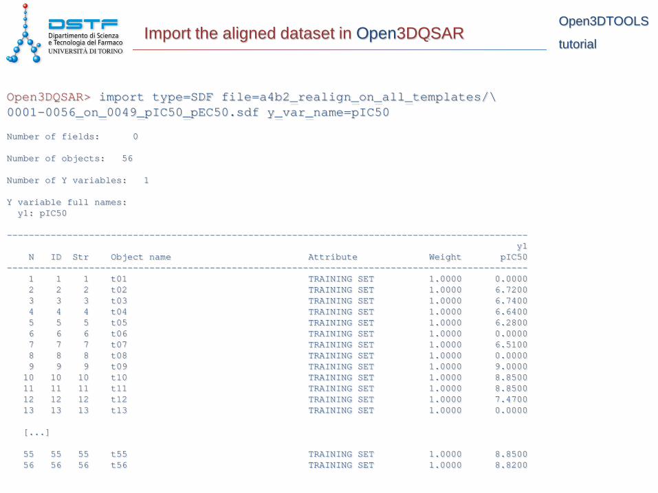
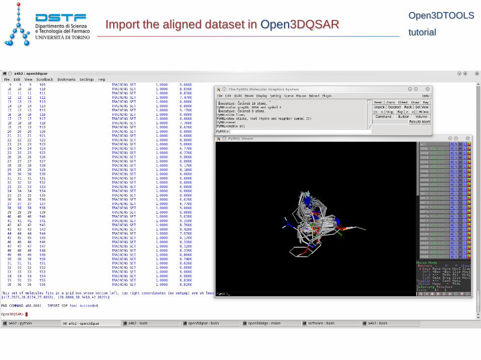
Open3DQSAR> import type=SDF file=a4b2_realign_on_all_templates/\ 0001-0056_on_0049_pIC50_pEC50.sdf y_var_name=pIC50
Number of fields: 0 Number of objects: 56 Number of Y variables: 1 Y variable full names: y1: pIC50 ----------------------------------------------------------------------------------------------- y1 N ID Str Object name Attribute Weight pIC50 ----------------------------------------------------------------------------------------------- 1 1 1 t01 TRAINING SET 1.0000 0.0000 2 2 2 t02 TRAINING SET 1.0000 6.7200 3 3 3 t03 TRAINING SET 1.0000 6.7400 4 4 4 t04 TRAINING SET 1.0000 6.6400 5 5 5 t05 TRAINING SET 1.0000 6.2800 6 6 6 t06 TRAINING SET 1.0000 0.0000 7 7 7 t07 TRAINING SET 1.0000 6.5100 8 8 8 t08 TRAINING SET 1.0000 0.0000 9 9 9 t09 TRAINING SET 1.0000 9.0000 10 10 10 t10 TRAINING SET 1.0000 8.8500 11 11 11 t11 TRAINING SET 1.0000 8.8500 12 12 12 t12 TRAINING SET 1.0000 7.4700 13 13 13 t13 TRAINING SET 1.0000 0.0000 [...] 55 55 55 t55 TRAINING SET 1.0000 8.8500 56 56 56 t56 TRAINING SET 1.0000 8.8200
Open3DTOOLS
tutorial Import the aligned dataset in Open3DQSAR

Open3DTOOLS
tutorial Remove objects for which pIC50 is not available
You may notice that activities are not available for all compounds; thus we ne need to remove from the dataset the compounds which have pIC50 set to 0.00
Open3DQSAR features a remove_object command which may serve this purpose; we only need a comma-separated list of the objects we wish to remove. This can be easily obtained with a BASH one-liner that you may type in another shell tab: $ grep -A1 pIC50 \ < a4b2_realign_on_all_templates/0001-0056_on_0049_pIC50_pEC50.sdf \ | grep -vE 'pIC50|\-\-' | cat -n | grep '0\.00$' \ | awk '{print $1}' | xargs | tr ' ' ','
1,6,8,13,14,16,17,20,21,27,30,31,32,33,34,35,39,52,53,54
And now type at the Open3DQSAR prompt:
Open3DQSAR> remove_object \ object_list=1,6,8,13,14,16,17,20,21,27,30,31,32,33,34,35,39,52,53,54
The PyMOL viewport will be updated to reflect the change.

Open3DTOOLS
tutorial Remove objects for which pIC50 is not available
Open3DTOOLS
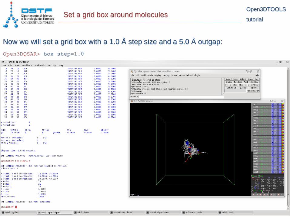
tutorial Set a grid box around molecules
Now we will set a grid box with a 1.0 Å step size and a 5.0 Å outgap: Open3DQSAR> box step=1.0
Open3DTOOLS
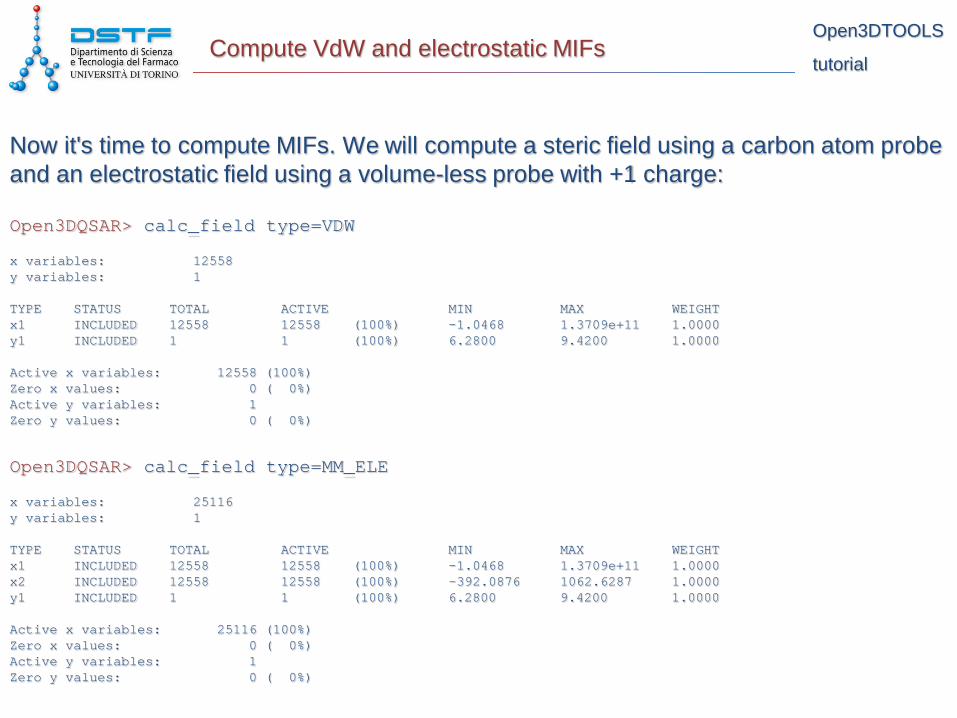
tutorial Compute VdW and electrostatic MIFs
Now it's time to compute MIFs. We will compute a steric field using a carbon atom probe and an electrostatic field using a volume-less probe with +1 charge:
Open3DQSAR> calc_field type=VDW
x variables: 12558 y variables: 1 TYPE STATUS TOTAL ACTIVE MIN MAX WEIGHT x1 INCLUDED 12558 12558 (100%) -1.0468 1.3709e+11 1.0000 y1 INCLUDED 1 1 (100%) 6.2800 9.4200 1.0000 Active x variables: 12558 (100%) Zero x values: 0 ( 0%) Active y variables: 1 Zero y values: 0 ( 0%)
Open3DQSAR> calc_field type=MM_ELE
x variables: 25116 y variables: 1 TYPE STATUS TOTAL ACTIVE MIN MAX WEIGHT x1 INCLUDED 12558 12558 (100%) -1.0468 1.3709e+11 1.0000 x2 INCLUDED 12558 12558 (100%) -392.0876 1062.6287 1.0000 y1 INCLUDED 1 1 (100%) 6.2800 9.4200 1.0000 Active x variables: 25116 (100%) Zero x values: 0 ( 0%) Active y variables: 1 Zero y values: 0 ( 0%)
Open3DTOOLS
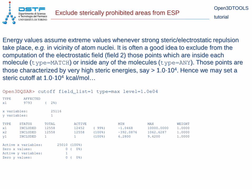
tutorial Exclude sterically prohibited areas from ESP
Energy values assume extreme values whenever strong steric/electrostatic repulsion take place, e.g. in vicinity of atom nuclei. It is often a good idea to exclude from the computation of the electrostatic field (field 2) those points which are inside each molecule (type=MATCH) or inside any of the molecules (type=ANY). Those points are those characterized by very high steric energies, say > 1.0·104. Hence we may set a steric cutoff at 1.0·104 kcal/mol…
Open3DQSAR> cutoff field_list=1 type=max level=1.0e04 TYPE AFFECTED x1 9793 ( 2%) x variables: 25116 y variables: 1 TYPE STATUS TOTAL ACTIVE MIN MAX WEIGHT x1 INCLUDED 12558 12452 ( 99%) -1.0468 10000.0000 1.0000 x2 INCLUDED 12558 12558 (100%) -392.0876 1062.6287 1.0000 y1 INCLUDED 1 1 (100%) 6.2800 9.4200 1.0000 Active x variables: 25010 (100%) Zero x values: 0 ( 0%) Active y variables: 1 Zero y values: 0 ( 0%)
Open3DTOOLS
tutorial Setting cutoffs
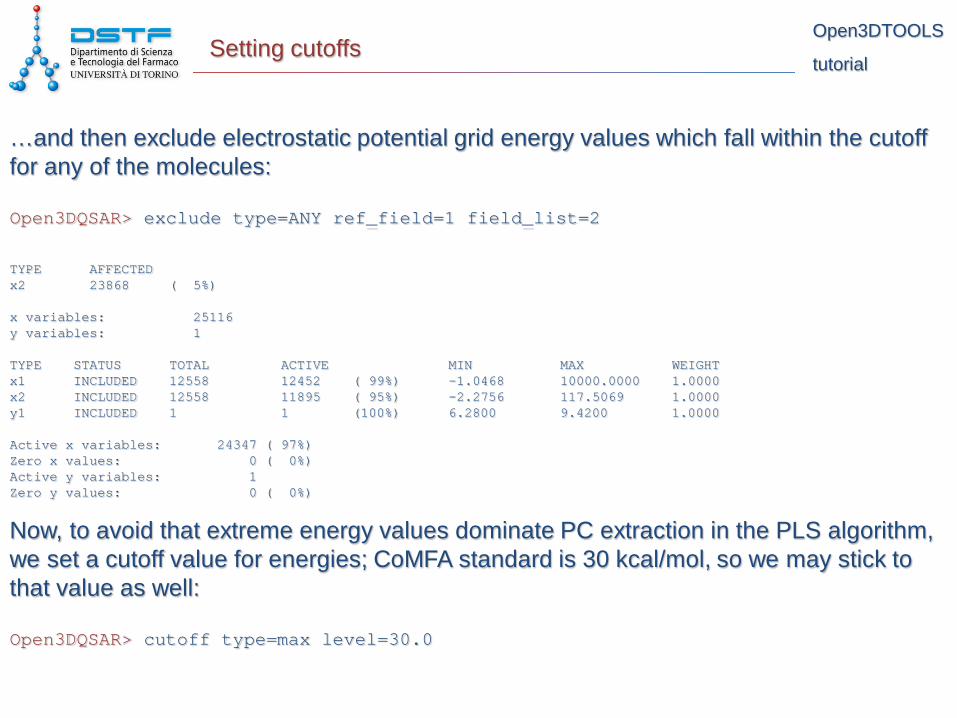
…and then exclude electrostatic potential grid energy values which fall within the cutoff for any of the molecules:
Open3DQSAR> exclude type=ANY ref_field=1 field_list=2
TYPE AFFECTED x2 23868 ( 5%) x variables: 25116 y variables: 1 TYPE STATUS TOTAL ACTIVE MIN MAX WEIGHT x1 INCLUDED 12558 12452 ( 99%) -1.0468 10000.0000 1.0000 x2 INCLUDED 12558 11895 ( 95%) -2.2756 117.5069 1.0000 y1 INCLUDED 1 1 (100%) 6.2800 9.4200 1.0000 Active x variables: 24347 ( 97%) Zero x values: 0 ( 0%) Active y variables: 1 Zero y values: 0 ( 0%)
Now, to avoid that extreme energy values dominate PC extraction in the PLS algorithm, we set a cutoff value for energies; CoMFA standard is 30 kcal/mol, so we may stick to that value as well:
Open3DQSAR> cutoff type=max level=30.0
Open3DTOOLS
tutorial Zeroing low energy values
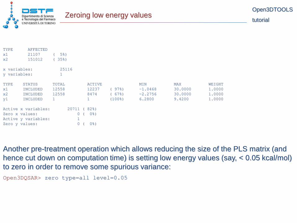
TYPE AFFECTED x1 21107 ( 5%) x2 151012 ( 35%) x variables: 25116 y variables: 1 TYPE STATUS TOTAL ACTIVE MIN MAX WEIGHT x1 INCLUDED 12558 12237 ( 97%) -1.0468 30.0000 1.0000 x2 INCLUDED 12558 8474 ( 67%) -2.2756 30.0000 1.0000 y1 INCLUDED 1 1 (100%) 6.2800 9.4200 1.0000 Active x variables: 20711 ( 82%) Zero x values: 0 ( 0%) Active y variables: 1 Zero y values: 0 ( 0%)
Another pre-treatment operation which allows reducing the size of the PLS matrix (and hence cut down on computation time) is setting low energy values (say, < 0.05 kcal/mol) to zero in order to remove some spurious variance: Open3DQSAR> zero type=all level=0.05

Open3DTOOLS
tutorial Split the dataset into training and test set
TYPE AFFECTED x1 353924 ( 80%) x2 0 ( 0%) x variables: 25116 y variables: 1 TYPE STATUS TOTAL ACTIVE MIN MAX WEIGHT x1 INCLUDED 12558 3893 ( 31%) -1.0468 30.0000 1.0000 x2 INCLUDED 12558 8474 ( 67%) -2.2756 30.0000 1.0000 y1 INCLUDED 1 1 (100%) 6.2800 9.4200 1.0000 Active x variables: 12367 ( 49%) Zero x values: 53540 ( 6%) Active y variables: 1 Zero y values: 0 ( 0%)
Now we need to split the dataset into a training and a test set (25% of the initial dataset size), so that we may assess the predictive power of the 3D-QSAR model on an external set of molecules which is completely independent of the model. What I did here was taking out of the training set one compound for each structural class:
Open3DQSAR> set id_list=7,10,15,25,37,40,42,46,55 attribute=testset
Open3DTOOLS
tutorial Split the dataset into training and test set
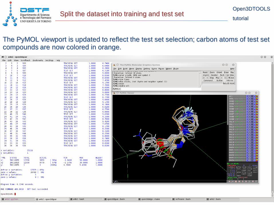
The PyMOL viewport is updated to reflect the test set selection; carbon atoms of test set compounds are now colored in orange.
Open3DTOOLS
tutorial SD cutoff
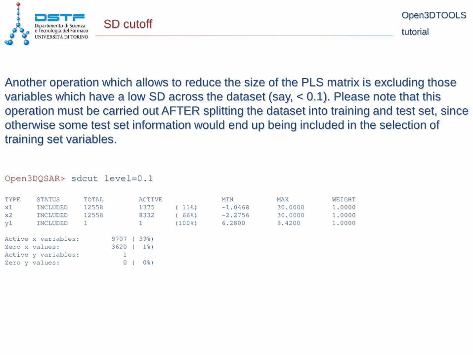
Another operation which allows to reduce the size of the PLS matrix is excluding those variables which have a low SD across the dataset (say, < 0.1). Please note that this operation must be carried out AFTER splitting the dataset into training and test set, since otherwise some test set information would end up being included in the selection of training set variables.
Open3DQSAR> sdcut level=0.1
TYPE STATUS TOTAL ACTIVE MIN MAX WEIGHT x1 INCLUDED 12558 1375 ( 11%) -1.0468 30.0000 1.0000 x2 INCLUDED 12558 8332 ( 66%) -2.2756 30.0000 1.0000 y1 INCLUDED 1 1 (100%) 6.2800 9.4200 1.0000 Active x variables: 9707 ( 39%) Zero x values: 3620 ( 1%) Active y variables: 1 Zero y values: 0 ( 0%)
Open3DTOOLS
tutorial N-level variable identification
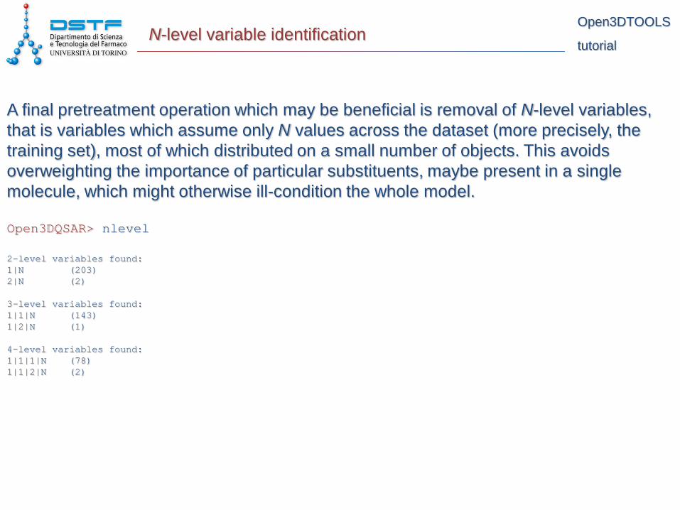
A final pretreatment operation which may be beneficial is removal of N-level variables, that is variables which assume only N values across the dataset (more precisely, the training set), most of which distributed on a small number of objects. This avoids overweighting the importance of particular substituents, maybe present in a single molecule, which might otherwise ill-condition the whole model.
Open3DQSAR> nlevel
2-level variables found: 1|N (203) 2|N (2) 3-level variables found: 1|1|N (143) 1|2|N (1) 4-level variables found: 1|1|1|N (78) 1|1|2|N (2)
Open3DTOOLS
tutorial N-level variable elimination
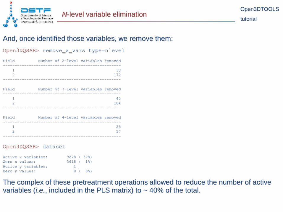
And, once identified those variables, we remove them: Open3DQSAR> remove_x_vars type=nlevel
Field Number of 2-level variables removed -------------------------------------------------- 1 33 2 172 -------------------------------------------------- Field Number of 3-level variables removed -------------------------------------------------- 1 40 2 104 -------------------------------------------------- Field Number of 4-level variables removed -------------------------------------------------- 1 23 2 57 --------------------------------------------------
Open3DQSAR> dataset
Active x variables: 9278 ( 37%) Zero x values: 3618 ( 1%) Active y variables: 1 Zero y values: 0 ( 0%)
The complex of these pretreatment operations allowed to reduce the number of active variables (i.e., included in the PLS matrix) to ~ 40% of the total.
Open3DTOOLS
tutorial Block Unscaled Weighting (BUW)
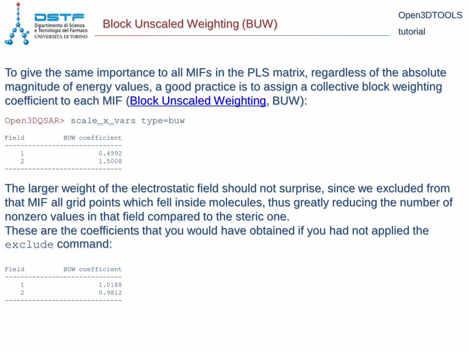
To give the same importance to all MIFs in the PLS matrix, regardless of the absolute magnitude of energy values, a good practice is to assign a collective block weighting coefficient to each MIF (Block Unscaled Weighting, BUW): Open3DQSAR> scale_x_vars type=buw
Field BUW coefficient ------------------------------ 1 0.4992 2 1.5008 ------------------------------
The larger weight of the electrostatic field should not surprise, since we excluded from that MIF all grid points which fell inside molecules, thus greatly reducing the number of nonzero values in that field compared to the steric one. These are the coefficients that you would have obtained if you had not applied the exclude command: Field BUW coefficient ------------------------------ 1 1.0188 2 0.9812 ------------------------------
Open3DTOOLS
tutorial Time for PLS
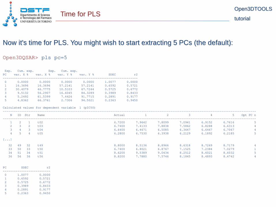
Now it's time for PLS. You might wish to start extracting 5 PCs (the default):
Open3DQSAR> pls pc=5
Exp. Cum. exp. Exp. Cum. exp. PC var. X % var. X % var. Y % var. Y % SDEC r2 -------------------------------------------------------------------------- 0 0.0000 0.0000 0.0000 0.0000 1.0077 0.0000 1 16.3696 16.3696 57.2141 57.2141 0.6592 0.5721 2 30.4079 46.7775 10.5103 67.7244 0.5725 0.6772 3 9.5132 56.2907 16.6045 84.3289 0.3989 0.8433 4 5.2492 61.5399 7.4426 91.7715 0.2891 0.9177 5 4.8362 66.3761 2.7306 94.5021 0.2363 0.9450 Calculated values for dependent variable 1 (pIC50) ------------------------------------------------------------------------------------------------------------------------------------------- N ID Str Name Actual 1 2 3 4 5 Opt PC n ------------------------------------------------------------------------------------------------------------------------------------------- 1 2 1 t02 6.7200 7.9642 7.8099 7.0941 6.9152 6.7616 5 2 3 2 t03 6.7400 7.4133 7.8838 7.5862 6.8288 6.6313 4 3 4 3 t04 6.6400 6.4671 6.5085 6.3647 6.6467 6.7067 4 4 5 4 t05 6.2800 6.7530 6.3938 6.2129 6.1892 6.2185 5
[...]
32 49 32 t49 8.8000 8.5136 8.8966 8.6318 8.7269 8.7179 4 33 50 33 t50 6.7400 6.8021 6.8767 7.1525 7.2384 7.0279 1 34 51 34 t51 8.6200 9.5389 9.0434 8.2512 8.6021 8.6032 5 36 56 36 t56 8.8200 7.7880 7.5746 8.1845 8.4893 8.4742 4 PC SDEC r2 -------------------------- 0 1.0077 0.0000 1 0.6592 0.5721 2 0.5725 0.6772 3 0.3989 0.8433 4 0.2891 0.9177 5 0.2363 0.9450
Open3DTOOLS
tutorial Calculated values output in SDF format
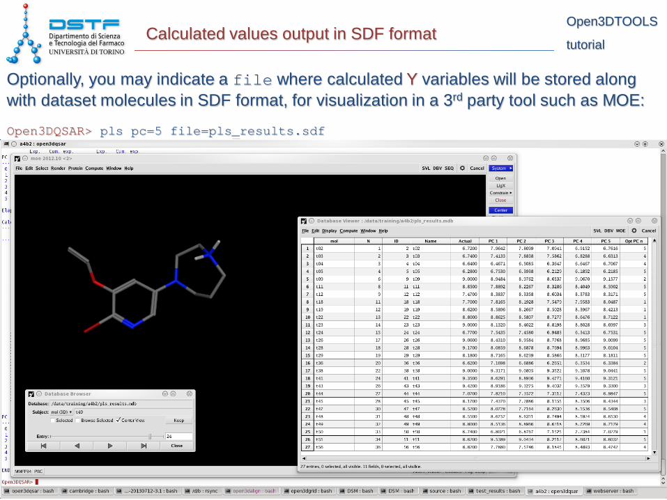
Optionally, you may indicate a file where calculated Y variables will be stored along with dataset molecules in SDF format, for visualization in a 3rd party tool such as MOE:
Open3DQSAR> pls pc=5 file=pls_results.sdf
Open3DTOOLS
tutorial External validation
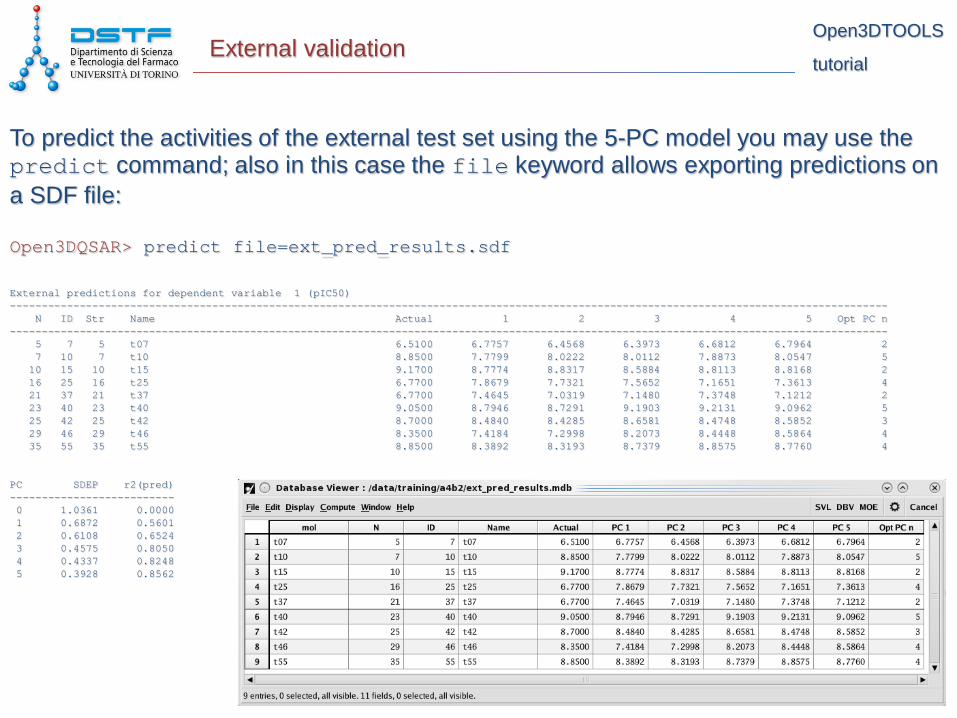
To predict the activities of the external test set using the 5-PC model you may use the predict command; also in this case the file keyword allows exporting predictions on a SDF file:
Open3DQSAR> predict file=ext_pred_results.sdf
External predictions for dependent variable 1 (pIC50) ------------------------------------------------------------------------------------------------------------------------------------------- N ID Str Name Actual 1 2 3 4 5 Opt PC n ------------------------------------------------------------------------------------------------------------------------------------------- 5 7 5 t07 6.5100 6.7757 6.4568 6.3973 6.6812 6.7964 2 7 10 7 t10 8.8500 7.7799 8.0222 8.0112 7.8873 8.0547 5 10 15 10 t15 9.1700 8.7774 8.8317 8.5884 8.8113 8.8168 2 16 25 16 t25 6.7700 7.8679 7.7321 7.5652 7.1651 7.3613 4 21 37 21 t37 6.7700 7.4645 7.0319 7.1480 7.3748 7.1212 2 23 40 23 t40 9.0500 8.7946 8.7291 9.1903 9.2131 9.0962 5 25 42 25 t42 8.7000 8.4840 8.4285 8.6581 8.4748 8.5852 3 29 46 29 t46 8.3500 7.4184 7.2998 8.2073 8.4448 8.5864 4 35 55 35 t55 8.8500 8.3892 8.3193 8.7379 8.8575 8.7760 4 PC SDEP r2(pred) -------------------------- 0 1.0361 0.0000 1 0.6872 0.5601 2 0.6108 0.6524 3 0.4575 0.8050 4 0.4337 0.8248 5 0.3928 0.8562

Open3DTOOLS
tutorial Variable grouping
Before looking at PLS coefficient isocontours, it will be beneficial to carry out a variable selection procedure in order to remove the less influent variables and obtain a more easily interpretable picture. Firstly we'll carry out variable grouping based on their closeness in 3D space with the Smart Region Definition algorithm:
Open3DQSAR> srd pc=5 collapse=yes critical_distance=1.0 \ collapse_distance=2.0 type=weights
Field Groups Vars in group 0 ------------------------------------- 1 727 11027 2 528 11582 Total 1255 22609 -------------------------------------
After grouping variables in the respective fields into Voronoi polyhedra, the latter are merged into larger ones: Collapsing Voronoi polyhedra. Field Initial groups Groups after collapsing ------------------------------------------------------- 1 727 621 2 528 54 Total 1255 675 -------------------------------------------------------

Open3DTOOLS
tutorial Variable selection
After grouping, a number of cross-validated models (using the LOO, LTO or LMO paradigms) are computed leaving in or out groups of variables according to a pattern determined by Fractional Factorial Design (FFD); the decision whether to keep or dismiss certain groups of variables in the final model depends on the change in CV performance connected with those groups:
Open3DQSAR> ffdsel pc=5 type=lmo runs=20 percent_dummies=20 use_srd_groups=yes \ combination_variable_ratio=1.0 fold_over=no Design matrix: 1024 combinations x 844 groups of variables (675 real, 169 dummy) Active variables not in group zero: 2073 Field Excluded Uncertain Fixed ----------------------------------------------------- 1 280 786 165 2 143 289 410 Total 423 1075 575 -----------------------------------------------------
Open3DQSAR> remove_x_vars type=ffdsel Field Number of x variables removed ----------------------------------------- 1 328 2 7300 -----------------------------------------
Open3DTOOLS
tutorial Model predictivity after variable selection
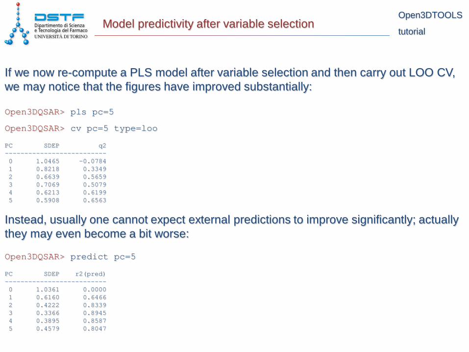
If we now re-compute a PLS model after variable selection and then carry out LOO CV, we may notice that the figures have improved substantially:
Open3DQSAR> pls pc=5
Open3DQSAR> cv pc=5 type=loo PC SDEP q2 -------------------------- 0 1.0465 -0.0784 1 0.8218 0.3349 2 0.6639 0.5659 3 0.7069 0.5079 4 0.6213 0.6199 5 0.5908 0.6563
Instead, usually one cannot expect external predictions to improve significantly; actually they may even become a bit worse: Open3DQSAR> predict pc=5 PC SDEP r2(pred) -------------------------- 0 1.0361 0.0000 1 0.6160 0.6466 2 0.4222 0.8339 3 0.3366 0.8945 4 0.3895 0.8587 5 0.4579 0.8047

Open3DTOOLS
tutorial Export PLS coefficients as grid maps
Finally, we output PLS coefficient grid maps for visualization in MOE, PyMOL or Maestro; the interpolate keyword allows obtaining smoother isocontours:
Open3DQSAR> pls pc=5
Open3DQSAR> export type=coefficients pc=5 file=MM_ffdsel_coefficients \ format=MOE interpolate=3
Open3DQSAR> export type=coefficients pc=5 file=MM_ffdsel_coefficients \ format=INSIGHT interpolate=3
Open3DQSAR> export type=coefficients pc=5 file=MM_ffdsel_coefficients \ format=MAESTRO interpolate=3
To visualize isocontours in MOE, you will need to load a SVL module upfront (included in your Open3DTOOLS installation):
Open3DTOOLS
tutorial Visualization of isocontours in MOE
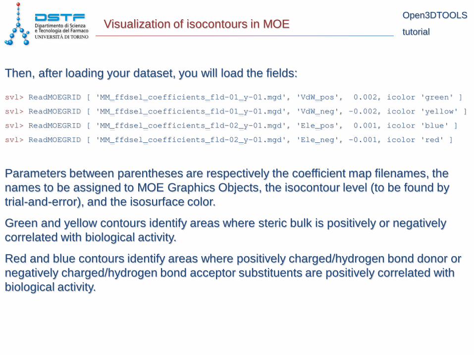
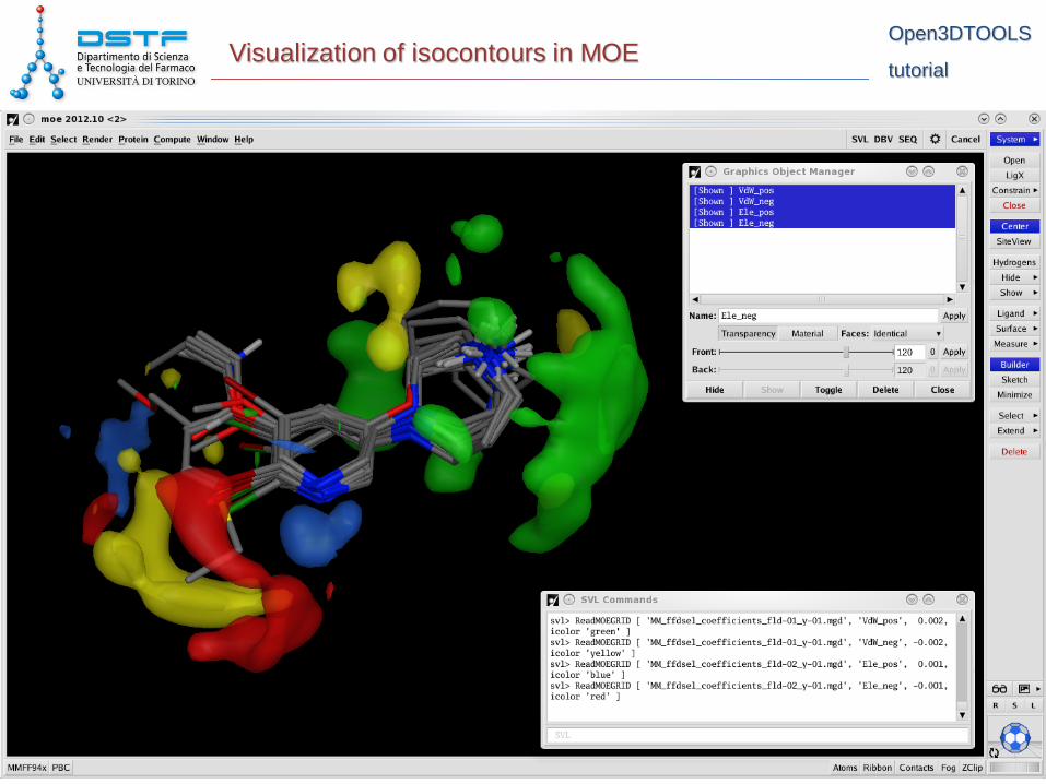
Then, after loading your dataset, you will load the fields:
svl> ReadMOEGRID [ 'MM_ffdsel_coefficients_fld-01_y-01.mgd', 'VdW_pos', 0.002, icolor 'green' ]
svl> ReadMOEGRID [ 'MM_ffdsel_coefficients_fld-01_y-01.mgd', 'VdW_neg', -0.002, icolor 'yellow' ]
svl> ReadMOEGRID [ 'MM_ffdsel_coefficients_fld-02_y-01.mgd', 'Ele_pos', 0.001, icolor 'blue' ]
svl> ReadMOEGRID [ 'MM_ffdsel_coefficients_fld-02_y-01.mgd', 'Ele_neg', -0.001, icolor 'red' ]
Parameters between parentheses are respectively the coefficient map filenames, the names to be assigned to MOE Graphics Objects, the isocontour level (to be found by trial-and-error), and the isosurface color.
Green and yellow contours identify areas where steric bulk is positively or negatively correlated with biological activity.
Red and blue contours identify areas where positively charged/hydrogen bond donor or negatively charged/hydrogen bond acceptor substituents are positively correlated with biological activity.
Open3DTOOLS
tutorial Visualization of isocontours in MOE
Open3DTOOLS
tutorial Visualization of isocontours in PyMOL
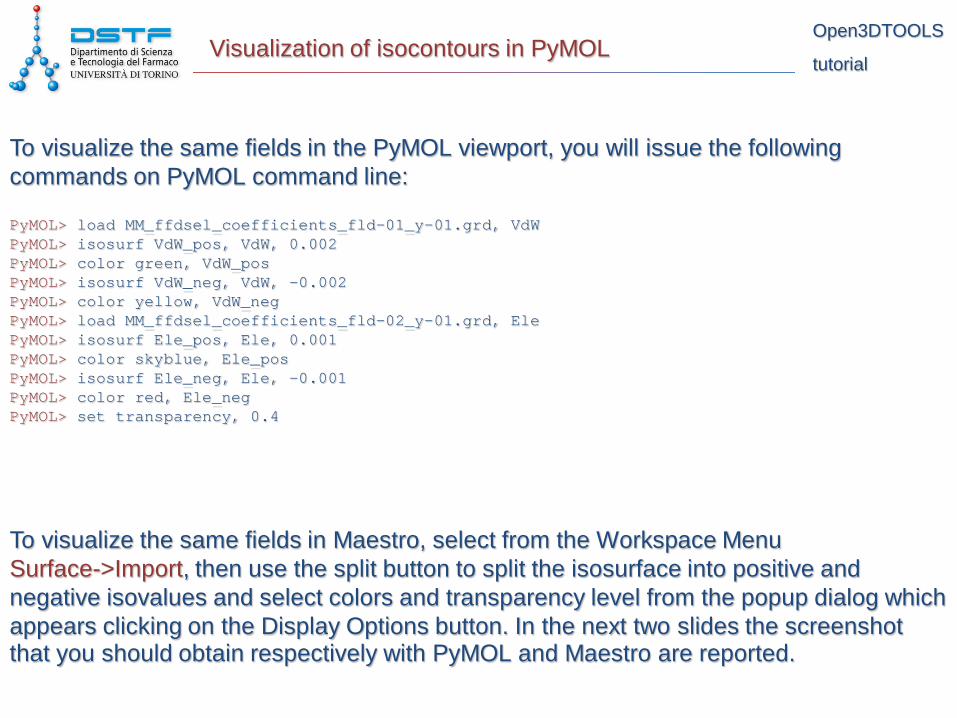
To visualize the same fields in the PyMOL viewport, you will issue the following commands on PyMOL command line:
PyMOL> load MM_ffdsel_coefficients_fld-01_y-01.grd, VdW PyMOL> isosurf VdW_pos, VdW, 0.002 PyMOL> color green, VdW_pos PyMOL> isosurf VdW_neg, VdW, -0.002 PyMOL> color yellow, VdW_neg PyMOL> load MM_ffdsel_coefficients_fld-02_y-01.grd, Ele PyMOL> isosurf Ele_pos, Ele, 0.001 PyMOL> color skyblue, Ele_pos PyMOL> isosurf Ele_neg, Ele, -0.001 PyMOL> color red, Ele_neg PyMOL> set transparency, 0.4
To visualize the same fields in Maestro, select from the Workspace Menu Surface->Import, then use the split button to split the isosurface into positive and negative isovalues and select colors and transparency level from the popup dialog which appears clicking on the Display Options button. In the next two slides the screenshot that you should obtain respectively with PyMOL and Maestro are reported.

Open3DTOOLS
tutorial Visualization of isocontours in PyMOL

Open3DTOOLS
tutorial Visualization of isocontours in Maestro
