opensees soil models and solid- fluid fully coupled elements · 2017-10-02 · opensees soil models...

OpenSees Soil Models and Solid-Fluid Fully Coupled Elements

User’s Manual

2008 ver 1.0

Zhaohui Yang, Jinchi Lu ([email protected]), and

Ahmed Elgamal ([email protected])

University of California, San Diego

Department of Structural Engineering

October 2008

Table of Contents

Introduction ............................................................................................................... 1

PressureDependMultiYield ...................................................................................... 1

PressureDependMultiYield02 .................................................................................. 7

PressureIndependMultiYield .................................................................................... 9

updateMaterialStage ............................................................................................... 13

updateMaterials ...................................................................................................... 14

parameter, addToParameter, and updateParameter ............................................ 15

FluidSolidPorousMaterial ....................................................................................... 17

FourNodeQuadUP ................................................................................................... 17

Nine_Four_Node_QuadUP ..................................................................................... 19

BrickUP .................................................................................................................... 21

Twenty_Eight_Node_BrickUP ................................................................................ 23

References .............................................................................................................. 25

1

This user manual describes the user interfaces for: 1) a number of NDMaterial models developed for simulating nonlinear, drained/undrained soil response under general 3D cyclic loading conditions, and 2) a number of 2D and 3D solid-fluid fully coupled elements for simulating pore water pressure dissipation/redistribution. Please visit http://cyclic.ucsd.edu/opensees for examples.

Notes:

1. To avoid numerical difficulties encountered when using the soil models, the following units are recommended:

SI units – use kilonewtons (kN), meters (m), tons (unit for mass), seconds English units – use pounds force (lbf), inches (in), seconds

2. The default values are in SI units.

Introduction

PressureDependMultiYield

http://cyclic.ucsd.edu/opensees

2

PressureDependMultiYield material is an elastic-plastic material for simulating the essential response characteristics of pressure sensitive soil materials under general loading conditions. Such characteristics include dilatancy (shear-induced volume contraction or dilation) and non-flow liquefaction (cyclic mobility), typically exhibited in sands or silts during monotonic or cyclic loading. Please visit http://cyclic.ucsd.edu/opensees for examples.

When this material is employed in regular solid elements (e.g., FourNodeQuad, Brick), it simulates drained soil response. To simulate soil response under fully undrained condition, this material may be either embedded in a FluidSolidPorousMaterial (see below), or used with one of the solid-fluid fully coupled elements (see below) with very low permeability. To simulate partially drained soil response, this material should be used with a solid-fluid fully coupled element with proper permeability values. During the application of gravity load (and static loads if any), material behavior is linear elastic. In the subsequent dynamic (fast) loading phase(s), the stress-strain response is elastic-plastic (see MATERIAL STAGE UPDATE below). Plasticity is formulated based on the multi-surface (nested surfaces) concept, with a non-associative flow rule to reproduce dilatancy effect. The yield surfaces are of the Drucker-Prager type. OUTPUT INTERFACE: The following information may be extracted for this material at a given integration point, using the OpenSees Element Recorder facility (McKenna and Fenves 2001): "stress", "strain", "backbone", or "tangent".

For 2D problems, the stress output follows this order: xx, yy, zz, xy, r, where r is the ratio between the shear (deviatoric) stress and peak shear strength at the current

confinement (0<=r<=1.0). The strain output follows this order: xx, yy, xy.

For 3D problems, the stress output follows this order: xx, yy, zz, xy, yz, zx, r, and

the strain output follows this order: xx, yy, zz, xy, yz, zx. The "backbone" option records (secant) shear modulus reduction curves at one or

more given confinements. The specific recorder command is as follows:

recorder Element –ele $eleNum -file $fName -dT $deltaT material $GaussNum backbone $p1 <$p2 …>

where p1, p2, … are the confinements at which modulus reduction curves are recorded. In the output file, corresponding to each given confinement there are two columns: shear

strain and secant modulus Gs. The number of rows equals the number of yield surfaces.

nDMaterial PressureDependMultiYield $tag $nd $rho $refShearModul $refBulkModul $frictionAng $peakShearStra $refPress $pressDependCoe $PTAng $contrac $dilat1 $dilat2 $liquefac1 $liquefac2 $liquefac3 <$noYieldSurf=20 <$r1 $Gs1 …> $e=0.6 $cs1=0.9 $cs2=0.02 $cs3=0.7 $pa=101 <$c=0.3>>


3

$Gr

Octahedral

shear stress

$f

Octahedral

shear strain

$max

Shear stress-strain at p'r

$tag A positive integer uniquely identifying the material among all nDMaterials.

$nd Number of dimensions, 2 for plane-strain, and 3 for 3D analysis.

$rho Saturated soil mass density.

$refShearModul (Gr)

Reference low-strain shear modulus, specified at a reference mean effective confining pressure refPress of p’r (see below).

$refBulkModul (Br) Reference bulk modulus, specified at a reference mean effective confining pressure refPress of p’r (see below).

$frictionAng () Friction angle at peak shear strength, in degrees.

$peakShearStra (max)

An octahedral shear strain at which the maximum shear strength is reached, specified at a reference mean effective confining pressure refPress of p’r (see below). Octahedral shear strain is defined as:

2/1222222

6663

2

xzyzxyzzxxzzyyyyxx

$refPress (p’r) Reference mean effective confining pressure at which Gr, Br, and max

are defined.

$pressDependCoe (d)

A positive constant defining variations of G and B as a function of

instantaneous effective confinement p’:

d

r

rp

pGG )(

d

r

rp

pBB )(

$PTAng (PT) Phase transformation angle, in degrees.

$contrac A non-negative constant defining the rate of shear-induced volume decrease (contraction) or pore pressure buildup. A larger value corresponds to faster contraction rate.

$dilat1, $dilat2 Non-negative constants defining the rate of shear-induced volume increase (dilation). Larger values correspond to stronger dilation rate.

4

$liquefac1, $liquefac2, $liquefac3

Parameters controlling the mechanism of liquefaction-induced perfectly plastic shear strain accumulation, i.e., cyclic mobility. Set liquefac1 = 0 to deactivate this mechanism altogether. liquefac1 defines the effective confining pressure (e.g., 10 kPa in SI units or 1.45 psi in English units) below which the mechanism is in effect. Smaller values should be assigned to denser sands. Liquefac2 defines the maximum amount of perfectly plastic shear strain developed at zero effective confinement during each loading phase. Smaller values should be assigned to denser sands. Liquefac3 defines the maximum amount of

biased perfectly plastic shear strain b accumulated at each loading

phase under biased shear loading conditions, as b=liquefac2 x

liquefac3. Typically, liquefac3 takes a value between 0.0 and 3.0. Smaller values should be assigned to denser sands. See the references listed at the end of this chapter for more information.

$noYieldSurf Number of yield surfaces, optional (must be less than 40, default is 20). The surfaces are generated based on the hyperbolic relation defined in Note 2 below.

$r $Gs Instead of automatic surfaces generation (Note 2), you can define yield surfaces directly based on desired shear modulus reduction curve. To do so, add a minus sign in front of noYieldSurf, then provide noYieldSurf pairs of shear strain () and modulus ratio (Gs) values. For example, to define 10 surfaces:

… -10 Gs1 … Gs10 … See Note 3 below for some important notes.

$e Initial void ratio, optional (default is 0.6).

$cs1, $cs2, $cs3, $pa

Parameters defining a straight critical-state line ec in e-p’ space. If cs3=0,

)/log(21 ac ppcscse

else (Li and Wang, JGGE, 124(12)),

3)/(21 csppcscse ac

where pa is atmospheric pressure for normalization (typically 101 kPa in SI units, or 14.65 psi in English units). All four constants are optional (default values: cs1=0.9, cs2=0.02, cs3=0.7, pa =101 kPa).

$c Numerical constant (default value = 0.3 kPa)

NOTE:

1. The friction angle defines the variation of peak (octahedral) shear strength f as a

function of current effective confinement p’:

pf

sin3

sin22

Octahedral shear stress is defined as:

2/1222222

6663

1

xzyzxyzzxxzzyyyyxx

2. (Automatic surface generation) At a constant confinement p’, the shear stress (octahedral) - shear strain (octahedral) nonlinearity is defined by a hyperbolic curve (backbone curve):

5

d

p

p

G

r

r

1

where r satisfies the following equation at p’r:

r

r

rf

Gp

/1sin3

sin22

max

max

3. (User defined surfaces) The user specified friction angle is ignored. Instead, is

defined as follows:

rm

rm

p

p

/36

/33sin

where m is the product of the last modulus and strain pair in the modulus reduction curve. Therefore, it is important to adjust the backbone curve so as to render an appropriate . If the resulting is smaller than the phase transformation angle PT, PT is set equal to .

Also remember that improper modulus reduction curves can result in strain softening response (negative tangent shear modulus), which is not allowed in the current model formulation. Finally, note that the backbone curve varies with confinement, although the variations are small within commonly interested confinement ranges. Backbone curves at different confinements can be obtained using the OpenSees element recorder facility (see OUTPUT INTERFACE above).

4. The last five optional parameters are needed when critical-state response (flow

liquefaction) is anticipated. Upon reaching the critical-state line, material dilatancy is set to zero.

5. SUGGESTED PARAMETER VALUES

6

For user convenience, a table is provided below as a quick reference for selecting parameter values. However, use of this table should be of great caution, and other information should be incorporated wherever possible.

Loose Sand (15%-35%)

Medium Sand (35%-65%)

Medium-dense Sand (65%-85%)

Dense Sand (85%-100%)

rho 1.7 ton/m3 or 1.59x10-4 (lbf)(s2)/in4

1.9 ton/m3 or 1.778x10-4 (lbf)(s2)/in4

2.0 ton/m3 or 1.872x10-4 (lbf)(s2)/in4

2.1 ton/m3 or 1.965x10-4 (lbf)(s2)/in4

refShearModul (at p’r=80 kPa or 11.6 psi)

5.5x104 kPa or 7.977x103 psi

7.5x104 kPa or 1.088x104 psi

1.0x105 kPa or 1.45x104 psi

1.3x105 kPa or 1.885x104 psi

refBulkModu (at p’r=80 kPa or 11.6 psi)

1.5x105 kPa or 2.176x104 psi

2.0x105 kPa or 2.9x104 psi

3.0x105 kPa or 4.351x104 psi

3.9x105 kPa or 5.656x104 psi

frictionAng 29 33 37 40

peakShearStra (at p’r=80 kPa or 11.6 psi)

0.1 0.1 0.1 0.1

refPress (p’r) 80 kPa or

11.6 psi

80 kPa or

11.6 psi

80 kPa or

11.6 psi

80 kPa or

11.6 psi

pressDependCoe 0.5 0.5 0.5 0.5

PTAng 29 27 27 27

contrac 0.21 0.07 0.05 0.03

dilat1 0. 0.4 0.6 0.8

dilat2 0 2 3 5

liquefac1 10 kPa or

1.45 psi

10 kPa or

1.45 psi

5 kPa or

0.725 psi

0

liquefac2 0.02 0.01 0.003 0

liquefac3 1 1 1 0

e 0.85 0.7 0.55 0.45

7

PressureDependMultiYield02 material is modified from PressureDependMultiYield

material, with: 1) additional parameters ($contrac3 and $dilat3) to account for K effect, 2) a parameter to account for the influence of previous dilation history on subsequent contraction phase ($contrac2), and 3) modified logic related to permanent shear strain accumulation ($liquefac1 and $liquefac2). Please visit http://cyclic.ucsd.edu/opensees for examples.

nDMaterial PressureDependMultiYield02 $tag $nd $rho $refShearModul $refBulkModul $frictionAng $peakShearStra $refPress $pressDependCoe $PTAng $contrac1 $contrac3 $dilat1 $dilat3 <$noYieldSurf=20 <$r1 $Gs1 …> $contrac2=5. $dilat2=3. $liquefac1=1. $liquefac2=0. $e=0.6 $cs1=0.9 $cs2=0.02 $cs3=0.7 $pa=101 <$c=0.1>>

$contrac3 A non-negative constant reflecting K effect.

$dilat3 A non-negative constant reflecting K effect.

$contrac2 A non-negative constant reflecting dilation history on contraction tendency.

$liquefac1 Damage parameter to define accumulated permanent shear strain as a function of dilation history. (Redefined and different from PressureDependMultiYield material).

$liquefac2 Damage parameter to define biased accumulation of permanent shear strain as a function of load reversal history. (Redefined and different from PressureDependMultiYield material).

$c Numerical constant (default value = 0.1 kPa)

Others See PressureDependMultiYield material above.

PressureDependMultiYield02


8

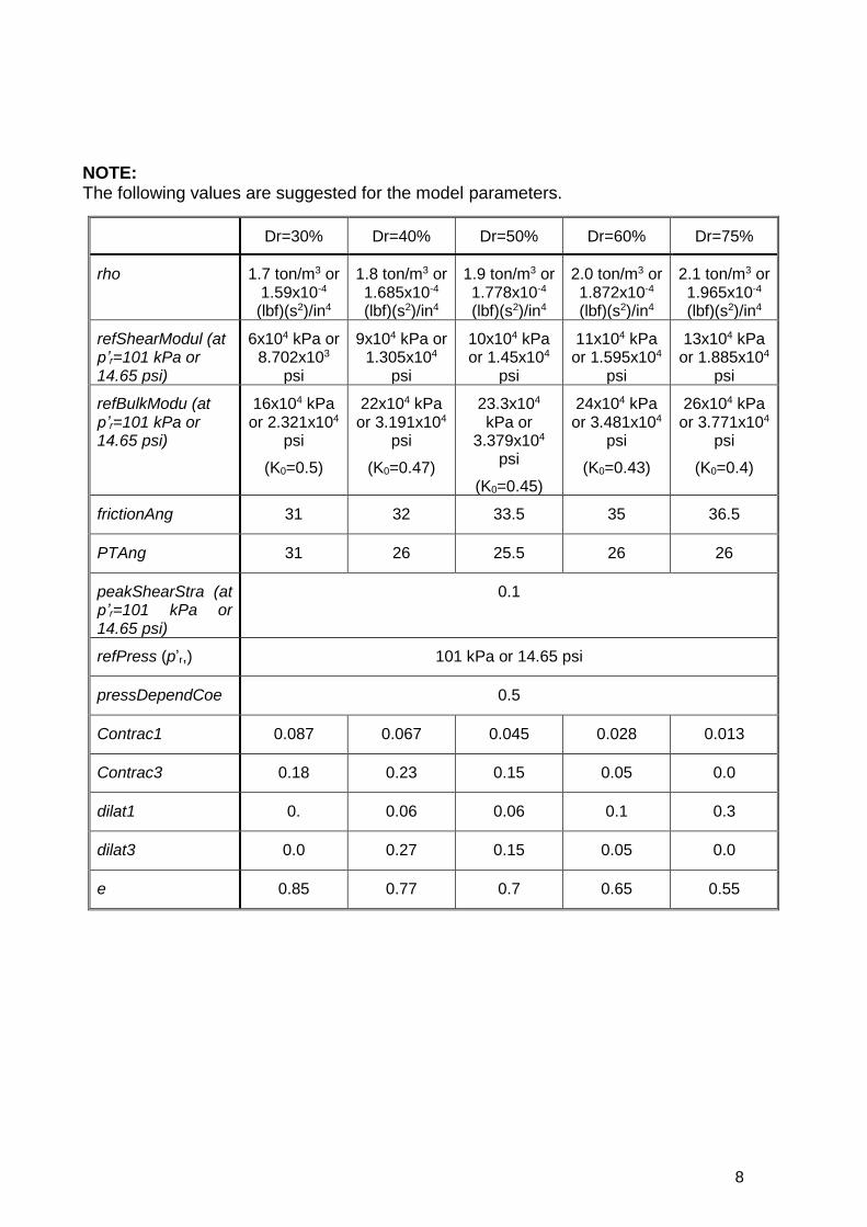
NOTE: The following values are suggested for the model parameters.

Dr=30% Dr=40% Dr=50% Dr=60% Dr=75%


1.8 ton/m3 or 1.685x10-4 (lbf)(s2)/in4

1.9 ton/m3 or 1.778x10-4 (lbf)(s2)/in4

2.0 ton/m3 or 1.872x10-4 (lbf)(s2)/in4

2.1 ton/m3 or 1.965x10-4 (lbf)(s2)/in4

refShearModul (at p’r=101 kPa or 14.65 psi)

6x104 kPa or 8.702x103

psi

9x104 kPa or 1.305x104

psi

10x104 kPa or 1.45x104

psi

11x104 kPa or 1.595x104

psi

13x104 kPa or 1.885x104

psi

refBulkModu (at p’r=101 kPa or 14.65 psi)

16x104 kPa or 2.321x104

psi

(K0=0.5)

22x104 kPa or 3.191x104

psi

(K0=0.47)

23.3x104 kPa or

3.379x104 psi

(K0=0.45)

24x104 kPa or 3.481x104

psi

(K0=0.43)

26x104 kPa or 3.771x104

psi

(K0=0.4)

frictionAng 31 32 33.5 35 36.5

PTAng 31 26 25.5 26 26

peakShearStra (at p’r=101 kPa or 14.65 psi)

0.1

refPress (p’r,) 101 kPa or 14.65 psi

pressDependCoe 0.5

Contrac1 0.087 0.067 0.045 0.028 0.013

Contrac3 0.18 0.23 0.15 0.05 0.0

dilat1 0. 0.06 0.06 0.1 0.3

dilat3 0.0 0.27 0.15 0.05 0.0

e 0.85 0.77 0.7 0.65 0.55

9

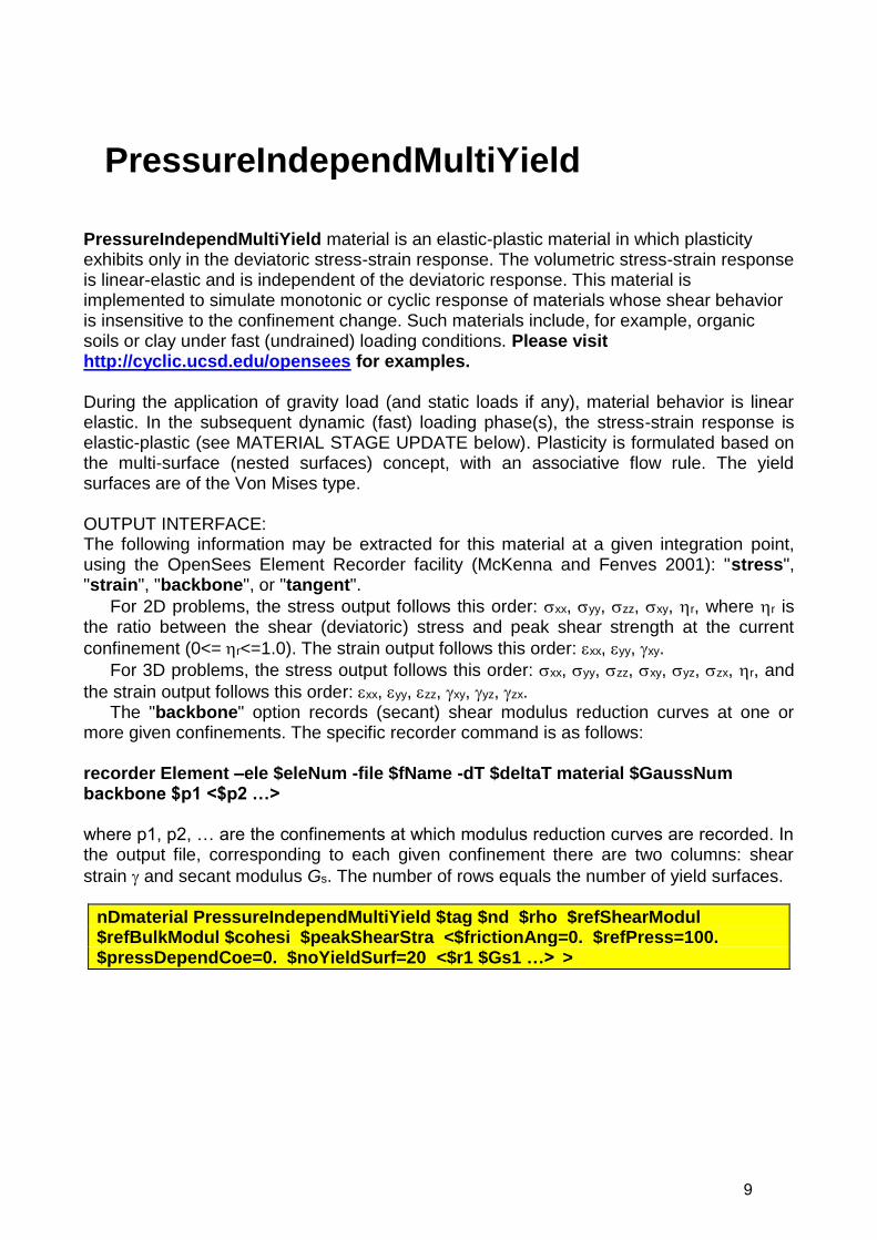
PressureIndependMultiYield material is an elastic-plastic material in which plasticity exhibits only in the deviatoric stress-strain response. The volumetric stress-strain response is linear-elastic and is independent of the deviatoric response. This material is implemented to simulate monotonic or cyclic response of materials whose shear behavior is insensitive to the confinement change. Such materials include, for example, organic soils or clay under fast (undrained) loading conditions. Please visit http://cyclic.ucsd.edu/opensees for examples. During the application of gravity load (and static loads if any), material behavior is linear elastic. In the subsequent dynamic (fast) loading phase(s), the stress-strain response is elastic-plastic (see MATERIAL STAGE UPDATE below). Plasticity is formulated based on the multi-surface (nested surfaces) concept, with an associative flow rule. The yield surfaces are of the Von Mises type. OUTPUT INTERFACE: The following information may be extracted for this material at a given integration point, using the OpenSees Element Recorder facility (McKenna and Fenves 2001): "stress", "strain", "backbone", or "tangent".

For 2D problems, the stress output follows this order: xx, yy, zz, xy, r, where r is the ratio between the shear (deviatoric) stress and peak shear strength at the current

confinement (0<=r<=1.0). The strain output follows this order: xx, yy, xy.

For 3D problems, the stress output follows this order: xx, yy, zz, xy, yz, zx, r, and

the strain output follows this order: xx, yy, zz, xy, yz, zx. The "backbone" option records (secant) shear modulus reduction curves at one or

more given confinements. The specific recorder command is as follows:

recorder Element –ele $eleNum -file $fName -dT $deltaT material $GaussNum backbone $p1 <$p2 …>

where p1, p2, … are the confinements at which modulus reduction curves are recorded. In the output file, corresponding to each given confinement there are two columns: shear

strain and secant modulus Gs. The number of rows equals the number of yield surfaces.

nDmaterial PressureIndependMultiYield $tag $nd $rho $refShearModul $refBulkModul $cohesi $peakShearStra <$frictionAng=0. $refPress=100. $pressDependCoe=0. $noYieldSurf=20 <$r1 $Gs1 …> >

PressureIndependMultiYield


10

$Gr

Octahedral

shear stress

$f

Octahedral

shear strain

$max

Shear stress-strain at p'r

$tag A positive integer uniquely identifying the material among all nDMaterials.

$nd Number of dimensions, 2 for plane-strain, and 3 for 3D analysis

$rho Saturated soil mass density.

$refShearModul (Gr)

Reference low-strain shear modulus, specified at a reference mean effective confining pressure refPress of p’r (see below).

$refBulkModul (Br) Reference bulk modulus, specified at a reference mean effective confining pressure refPress of p’r (see below).

$cohesi (c) Apparent cohesion at zero effective confinement.

$peakShearStra

(max)

An octahedral shear strain at which the maximum shear strength is reached, specified at a reference mean effective confining pressure refPress of p’r (see below).

$frictionAng () Friction angle at peak shear strength in degrees, optional (default is 0.0).

$refPress (p’r) Reference mean effective confining pressure at which Gr, Br, and max are defined, optional (default is 100. kPa).

$pressDependCoe (d)

An optional non-negative constant defining variations of G and B as a function of initial effective confinement p’i (default is 0.0):

d

r

i

rp

pGG )(

d

r

i

rp

pBB )(

If =0, d is reset to 0.0.

$noYieldSurf Number of yield surfaces, optional (must be less than 40, default is 20). The surfaces are generated based on the hyperbolic relation defined in Note 2 below.

$r $Gs Instead of automatic surfaces generation (Note 2), you can define yield surfaces directly based on desired shear modulus reduction curve. To do so, add a minus sign in front of noYieldSurf, then provide

noYieldSurf pairs of shear strain () and modulus ratio (Gs) values. For example, to define 10 surfaces:

… -10 Gs1 … Gs10 … See Note 3 below for some important notes.

NOTE:

1. The friction angle and cohesion c define the variation of peak (octahedral) shear

strength f as a function of initial effective confinement p’i :

11

cpif3

22

sin3

sin22

2. Automatic surface generation: at a constant confinement p’, the shear stress

(octahedral) - shear strain (octahedral) nonlinearity is defined by a hyperbolic curve (backbone curve):

d

p

p

G

r

r

1

where r satisfies the following equation at p’r :

r

r

rf

Gcp

/13

22

sin3

sin22

max

max

3. (User defined surfaces) If the user specifies =0, cohesion c will be ignored.

Instead, c is defined by c=sqrt(3)*m/2, where m is the product of the last modulus and strain pair in the modulus reduction curve. Therefore, it is important to adjust the backbone curve so as to render an appropriate c.

If the user specifies , this will be ignored. Instead, is defined as follows:

rm

rm

pc

pc

/)23(6

/)23(3sin

If the resulting <0, we set =0 and c=sqrt(3)*m/2. Also remember that improper modulus reduction curves can result in strain

softening response (negative tangent shear modulus), which is not allowed in the current model formulation. Finally, note that the backbone curve varies with confinement, although the variation is small within commonly interested confinement ranges. Backbone curves at different confinements can be obtained using the OpenSees element recorder facility (see OUTPUT INTERFACE above).

12

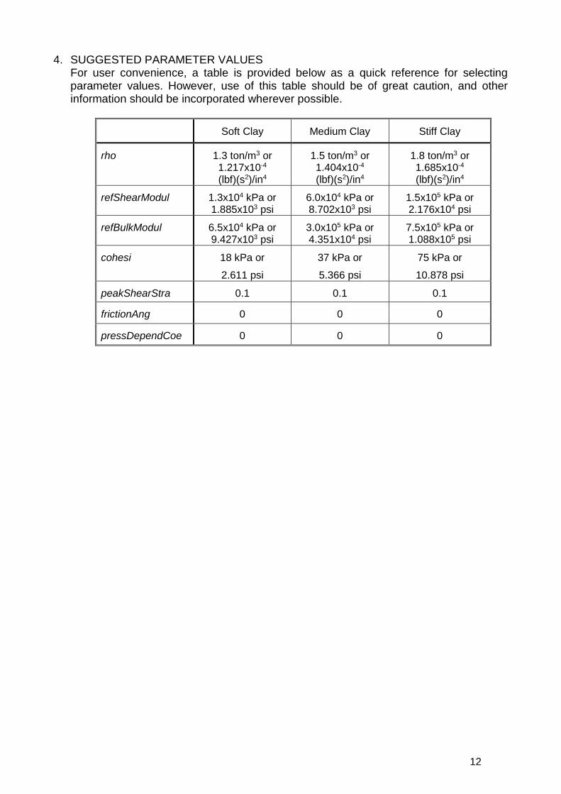
4. SUGGESTED PARAMETER VALUES For user convenience, a table is provided below as a quick reference for selecting parameter values. However, use of this table should be of great caution, and other information should be incorporated wherever possible.

Soft Clay Medium Clay Stiff Clay


1.5 ton/m3 or 1.404x10-4 (lbf)(s2)/in4

1.8 ton/m3 or 1.685x10-4 (lbf)(s2)/in4

refShearModul 1.3x104 kPa or 1.885x103 psi

6.0x104 kPa or 8.702x103 psi

1.5x105 kPa or 2.176x104 psi

refBulkModul 6.5x104 kPa or 9.427x103 psi

3.0x105 kPa or 4.351x104 psi

7.5x105 kPa or 1.088x105 psi

cohesi 18 kPa or

2.611 psi

37 kPa or

5.366 psi

75 kPa or

10.878 psi

peakShearStra 0.1 0.1 0.1

frictionAng 0 0 0

pressDependCoe 0 0 0

13

This command is used to update a PressureDependMultiYield, PressureDependMultiYield02, PressureIndependMultiYield, or FluidSolidPorous material. To conduct a seismic analysis, two stages should be followed. First, during the application of gravity load (and static loads if any), set material stage to 0, and material behavior is linear elastic (with Gr and Br as elastic moduli). A FluidSolidPorous material does not contribute to the material response if its stage is set to 0. After the application of gravity load, set material stage to 1 or 2. In case of stage 2, all the elastic material properties are then internally determined at the current effective confinement, and remain constant thereafter. In the subsequent dynamic (fast) loading phase(s), the deviatoric stress-strain response is elastic-plastic (stage 1) or linear-elastic (stage 2), and the volumetric response remains linear-elastic. Please visit http://cyclic.ucsd.edu/opensees for examples.

updateMaterialStage -material $tag -stage $sNum

$tag Material number.

$sNum desired stage: 0 - linear elastic, 1 – plastic, 2 - Linear elastic, with elasticity constants (shear modulus and bulk modulus) as a function of initial effective confinement.

Notes:

1) The updateMaterialStage command cannot occur until elements have been built.

2) By default, the updateMaterialStage command starts at stage 0.

updateMaterialStage


14

This command is used to update the parameters of PressureDependMultiYield or PressureIndependMultiYield material. Currently, two material parameters, reference low-strain shear modulus Gr and reference bulk modulus Br, can be modified during an analysis.

Please visit http://cyclic.ucsd.edu/opensees for examples.

updateMaterials -material $tag shearModulus $newVal

updateMaterials -material $tag bulkModulus $newVal

$tag Material number.

$newVal New parameter value.

updateMaterials


15

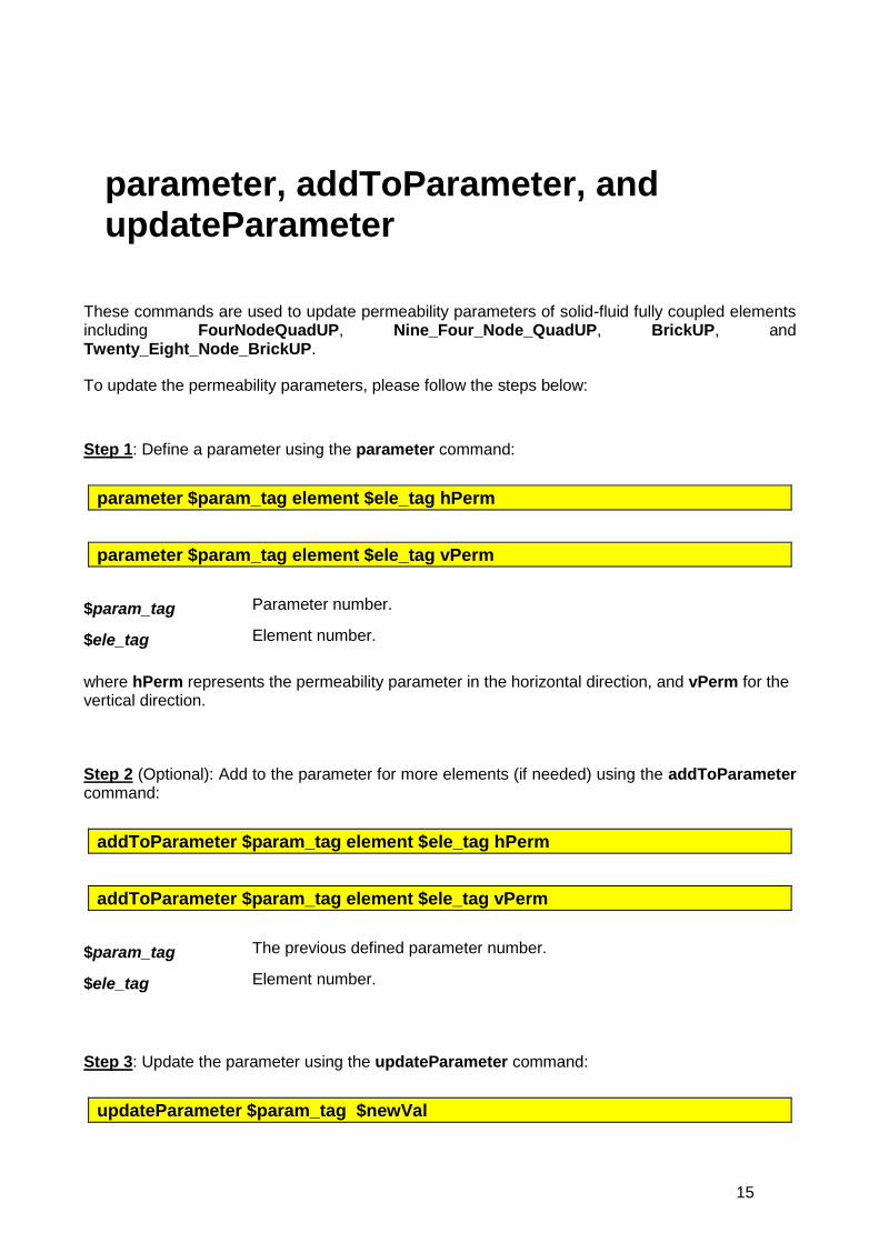
These commands are used to update permeability parameters of solid-fluid fully coupled elements including FourNodeQuadUP, Nine_Four_Node_QuadUP, BrickUP, and Twenty_Eight_Node_BrickUP.

To update the permeability parameters, please follow the steps below:

Step 1: Define a parameter using the parameter command:

parameter $param_tag element $ele_tag hPerm

parameter $param_tag element $ele_tag vPerm

$param_tag Parameter number.

$ele_tag Element number.

where hPerm represents the permeability parameter in the horizontal direction, and vPerm for the vertical direction.

Step 2 (Optional): Add to the parameter for more elements (if needed) using the addToParameter command:

addToParameter $param_tag element $ele_tag hPerm

addToParameter $param_tag element $ele_tag vPerm

$param_tag The previous defined parameter number.

$ele_tag Element number.

Step 3: Update the parameter using the updateParameter command:

updateParameter $param_tag $newVal

parameter, addToParameter, and updateParameter

16

$param_tag The previous defined parameter number.

$newVal New parameter value.

Example: … parameter 1 element 1 hPerm addToParameter 1 element 2 hPerm … updateParameter 1 1e-5 …

17

FluidSolidPorousMaterial couples the responses of two phases: fluid and solid. The fluid phase response is only volumetric and linear elastic. The solid phase can be any NDMaterial. This material is developed to simulate the response of saturated porous media under fully undrained condition. Please visit http://cyclic.ucsd.edu/opensees for examples.

OUTPUT INTERFACE: The following information may be extracted for this material at given integration point, using the OpenSees Element Recorder facility (McKenna and Fenves 2001): "stress", "strain", "tangent", or "pressure". The "pressure" option records excess pore pressure and excess pore pressure ratio at a given material integration point.

nDMaterial FluidSolidPorousMaterial $tag $nd $soilMatTag $combinedBulkModul <$pa=101>

$tag A positive integer uniquely identifying the material among all nDMaterials

$nd Number of dimensions, 2 for plane-strain, and 3 for general 3D analysis.

$soilMatTag The material number for the solid phase material (previously defined).

$combinBulkModul Combined undrained bulk modulus Bc relating changes in pore pressure and volumetric strain, may be approximated by:

nBB fc /

where Bf is the bulk modulus of fluid phase (2.2x106 kPa (or 3.191x105 psi) for water typically), and n the initial porosity.

$pa Optional atmospheric pressure for normalization (typically 101 kPa in SI units, or 14.65 psi in English units)

NOTE:

1. Buoyant unit weight (total unit weight - fluid unit weight) should be used in definition of the finite elements composed of a FluidSolidPorousMaterial.

2. During the application of gravity (elastic) load, the fluid phase does not contribute to the material response.

FluidSolidPorousMaterial

FourNodeQuadUP


18

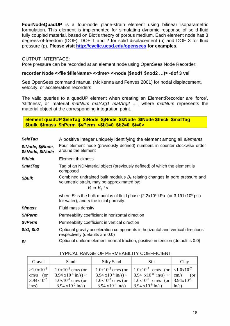
FourNodeQuadUP is a four-node plane-strain element using bilinear isoparametric formulation. This element is implemented for simulating dynamic response of solid-fluid fully coupled material, based on Biot's theory of porous medium. Each element node has 3 degrees-of-freedom (DOF): DOF 1 and 2 for solid displacement (u) and DOF 3 for fluid pressure (p). Please visit http://cyclic.ucsd.edu/opensees for examples.

OUTPUT INTERFACE: Pore pressure can be recorded at an element node using OpenSees Node Recorder:

recorder Node <-file $fileName> <-time> <-node ($nod1 $nod2 …)> -dof 3 vel

See OpenSees command manual (McKenna and Fenves 2001) for nodal displacement, velocity, or acceleration recorders. The valid queries to a quadUP element when creating an ElementRecorder are 'force', 'stiffness', or 'material matNum matArg1 matArg2 ...', where matNum represents the material object at the corresponding integration point.

element quadUP $eleTag $iNode $jNode $kNode $lNode $thick $matTag $bulk $fmass $hPerm $vPerm <$b1=0 $b2=0 $t=0>

$eleTag A positive integer uniquely identifying the element among all elements

$iNode, $jNode, $kNode, $lNode

Four element node (previously defined) numbers in counter-clockwise order around the element

$thick Element thickness

$matTag Tag of an NDMaterial object (previously defined) of which the element is composed

$bulk Combined undrained bulk modulus Bc relating changes in pore pressure and volumetric strain, may be approximated by:

nBB fc /

where Bf is the bulk modulus of fluid phase (2.2x106 kPa (or 3.191x105 psi) for water), and n the initial porosity.

$fmass Fluid mass density

$hPerm Permeability coefficient in horizontal direction

$vPerm Permeability coefficient in vertical direction

$b1, $b2 Optional gravity acceleration components in horizontal and vertical directions respectively (defaults are 0.0)

$t Optional uniform element normal traction, positive in tension (default is 0.0)

TYPICAL RANGE OF PERMEABILITY COEFFICIENT

Gravel Sand Silty Sand Silt Clay

>1.0x10-1

cm/s (or

3.94x10-2

in/s)

1.0x10-3 cm/s (or

3.94 x10-4 in/s) ~

1.0x10-1 cm/s (or

3.94 x10-2 in/s)

1.0x10-5 cm/s (or

3.94 x10-6 in/s) ~

1.0x10-3 cm/s (or

3.94 x10-4 in/s)

1.0x10-7 cm/s (or

3.94 x10-8 in/s) ~

1.0x10-5 cm/s (or

3.94 x10-6 in/s)

<1.0x10-7

cm/s (or

3.94x10-8

in/s)


19

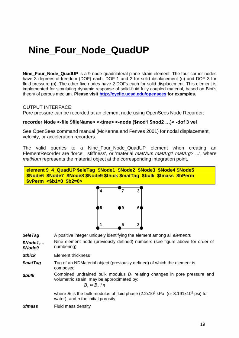
Nine_Four_Node_QuadUP is a 9-node quadrilateral plane-strain element. The four corner nodes have 3 degrees-of-freedom (DOF) each: DOF 1 and 2 for solid displacement (u) and DOF 3 for fluid pressure (p). The other five nodes have 2 DOFs each for solid displacement. This element is implemented for simulating dynamic response of solid-fluid fully coupled material, based on Biot's theory of porous medium. Please visit http://cyclic.ucsd.edu/opensees for examples.



See OpenSees command manual (McKenna and Fenves 2001) for nodal displacement, velocity, or acceleration recorders. The valid queries to a Nine_Four_Node_QuadUP element when creating an ElementRecorder are 'force', 'stiffness', or 'material matNum matArg1 matArg2 ...', where matNum represents the material object at the corresponding integration point.

element 9_4_QuadUP $eleTag $Node1 $Node2 $Node3 $Node4 $Node5 $Node6 $Node7 $Node8 $Node9 $thick $matTag $bulk $fmass $hPerm $vPerm <$b1=0 $b2=0>

21

34

5

6

7

8 9


$Node1,… $Node9

Nine element node (previously defined) numbers (see figure above for order of numbering).

$thick Element thickness



nBB fc /



Nine_Four_Node_QuadUP


20

$hPerm, $vPerm

Permeability coefficient in horizontal and vertical directions respectively.

$b1, $b2 Optional gravity acceleration components in horizontal and vertical directions respectively (defaults are 0.0)

21

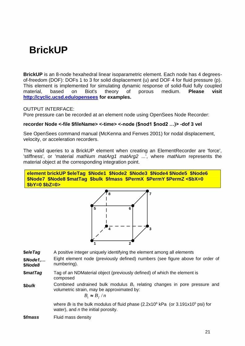
BrickUP is an 8-node hexahedral linear isoparametric element. Each node has 4 degrees-of-freedom (DOF): DOFs 1 to 3 for solid displacement (u) and DOF 4 for fluid pressure (p). This element is implemented for simulating dynamic response of solid-fluid fully coupled material, based on Biot's theory of porous medium. Please visit http://cyclic.ucsd.edu/opensees for examples.



See OpenSees command manual (McKenna and Fenves 2001) for nodal displacement, velocity, or acceleration recorders. The valid queries to a BrickUP element when creating an ElementRecorder are 'force', 'stiffness', or 'material matNum matArg1 matArg2 ...', where matNum represents the material object at the corresponding integration point.

element brickUP $eleTag $Node1 $Node2 $Node3 $Node4 $Node5 $Node6 $Node7 $Node8 $matTag $bulk $fmass $PermX $PermY $PermZ <$bX=0 $bY=0 $bZ=0>

21

34

6

78

5


$Node1,… $Node8

Eight element node (previously defined) numbers (see figure above for order of numbering).



nBB fc /



BrickUP


22

$permX, $permY, $permZ

Permeability coefficients in x, y, and z directions respectively.

$bX, $bY, $bZ

Optional gravity acceleration components in x, y, and z directions directions respectively (defaults are 0.0)

23

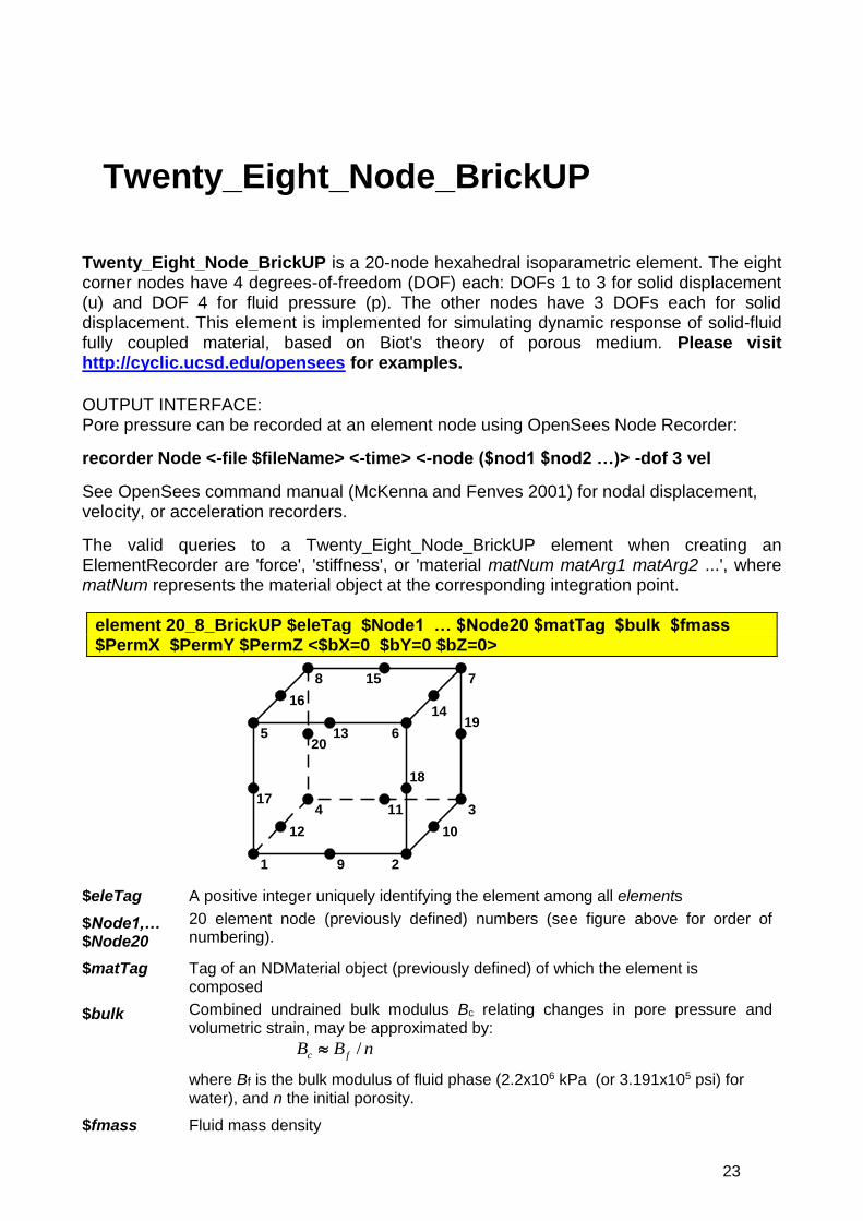
Twenty_Eight_Node_BrickUP is a 20-node hexahedral isoparametric element. The eight corner nodes have 4 degrees-of-freedom (DOF) each: DOFs 1 to 3 for solid displacement (u) and DOF 4 for fluid pressure (p). The other nodes have 3 DOFs each for solid displacement. This element is implemented for simulating dynamic response of solid-fluid fully coupled material, based on Biot's theory of porous medium. Please visit http://cyclic.ucsd.edu/opensees for examples.



See OpenSees command manual (McKenna and Fenves 2001) for nodal displacement, velocity, or acceleration recorders.

The valid queries to a Twenty_Eight_Node_BrickUP element when creating an ElementRecorder are 'force', 'stiffness', or 'material matNum matArg1 matArg2 ...', where matNum represents the material object at the corresponding integration point.

element 20_8_BrickUP $eleTag $Node1 … $Node20 $matTag $bulk $fmass $PermX $PermY $PermZ <$bX=0 $bY=0 $bZ=0>

21

34

6

78

5

9

10

11

12

13

14

15

16

17

18

19

20


$Node1,… $Node20

20 element node (previously defined) numbers (see figure above for order of numbering).



nBB fc /



Twenty_Eight_Node_BrickUP


24

$permX, $permY, $permZ

Permeability coefficients in x, y, and z directions respectively.

$bX, $bY, $bZ

Optional gravity acceleration components in x, y, and z directions directions respectively (defaults are 0.0)

25

Elgamal, A., Lai, T., Yang, Z. and He, L. (2001). "Dynamic Soil Properties, Seismic Downhole Arrays and Applications in Practice," State-of-the-art paper, Proc., 4th Intl. Conf. on Recent Advances in Geote. E.Q. Engrg. Soil Dyn. March 26-31, San Diego, CA, S. Prakash (Ed.).

Elgamal, A., Yang, Z. and Parra, E. (2002). "Computational Modeling of Cyclic Mobility and Post-Liquefaction Site Response," Soil Dyn. Earthquake Engrg., 22(4), 259-271.

Elgamal, A., Yang, Z., Parra, E. and Ragheb, A. (2003). "Modeling of Cyclic Mobility in Saturated Cohesionless Soils," Int. J. Plasticity, 19(6), 883-905.

McKenna, F. and Fenves, G. (2001). "The OpenSees Command Language Manual: version 1.2," Pacific Earthquake Engineering Center, Univ. of Calif., Berkeley. (http://opensees.berkeley.edu).

Parra, E. (1996). "Numerical Modeling of Liquefaction and Lateral Ground Deformation Including Cyclic Mobility and Dilation Response in Soil Systems," Ph.D. Thesis, Dept. of Civil Engineering, Rensselaer Polytechnic Institute, Troy, NY.

Yang, Z. (2000). "Numerical Modeling of Earthquake Site Response Including Dilation and Liquefaction," Ph.D. Thesis, Dept. of Civil Engineering and Engineering Mechanics, Columbia University, NY, New York.

Yang, Z. and Elgamal, A. (2002). "Influence of Permeability on Liquefaction-Induced Shear Deformation," J. Engrg. Mech., ASCE, 128(7), 720-729. Yang, Z., Elgamal, A. and Parra, E. (2003). "A Computational Model for Liquefaction and Associated Shear Deformation," J. Geotechnical and Geoenvironmental Engineering, ASCE, 129(12), 1119-1127.

References

opensees soil models and solid- fluid fully coupled elements · 2017-10-02 · opensees soil models...

Documents