operating systems “memory...

Operating Systems“Memory Management”

Mathieu DelalandreUniversity of Tours, Tours city, France

[email protected] 12, 2019

1


1. Introduction

2. Contiguous memory allocation

2.1. Partitioning and placement algorithms

2.2. Memory fragmentation and compaction

2.3. Process swapping

2.4. Loading, address binding and protection

3. Simple paging and segmentation

3.1. Paging, basic method

3.2. Segmentation

2

Introduction (1)

3

As one goes down in the hierarchy, the following occurs:a. decreasing cost per bit.b. increasing capacity.c. increasing access time.d. decreasing frequency of access to the memory by the

processor.

Memory hierarchy: memory is a major component in any computer. Ideally, memory should be extremely fast (faster than executing an instruction on CPU), abundantly large and dirt chip. No current technology satisfies all these goals, so a different approach is taken. The memory system is constructed as a hierarchy of layers.

Access time(4KB)

Capacity

Registers 0.25 - 0.5 ns < 1 KB

Cache 0.5 - 25 ns > 16 MB

Main memory 80 - 250 ns > 16 GB

Disk storage 30 µs - plus > 100 GB

i.e. from 130.2 Mb.s-1 to 15.6 Gb.s-1

Introduction (2)

4

( ) ( )211 1 TTHTHT +×−+×=

The strategy of using a memory hierarchy works in principle, but only if conditions (a) through (d) in the preceding list apply.

e.g. with a two-level memory hierarchyH is the hit ratio, the faction of all memory accesses that are

found in the faster memory.T1 is the access time to level 1.T2 is the access time to level 2.

is the average access time, computed as:T

T1

T2

T1+T2

0 1

Average access time

Hit ratio (H)

( )T


T1/T2

Access time(4KB)

Capacity


Cache 0.5 - 25 ns > 16 MB



i.e. from 130.2 Mb.s-1 to 15.6 Gb.s-1

Introduction (3)

5

The strategy of using a memory hierarchy works in principle, but only if conditions (a) through (d) in the preceding list apply.

e.g. with a two-level memory hierarchyConsidering 200 ns / 40 µs as access times to the main / disk memory,

For a performance degradation less than 10 percent in main memory,

then, 1 fault access out of 1990.additional constraints must be considered, a typical hard disk has:

( ) 41041200 ××−+×= HHT

( )0,999497

1041200220 4

=××−+×=

H

HH

Latency 3 ms

Seek time 5 ms

Access time 0.05 ms

Total ≈8 ms


Access time(4KB)

Capacity


Cache 0.5 - 25 ns > 16 MB



i.e. from 130.2 Mb.s-1 to 15.6 Gb.s-1

Introduction (4)

6

Memory management: managing the lowest level of cache memory is normally done by hardware, the focus of memory management is on the programmer’s model of main memory and how it can be managed well.

Memory management without memory abstraction: the simplest memory management is without abstraction. Main memory is generally divided in two parts, one part for the operating system and one part for the program currently executed. The model of memory presented to the programmer was physical memory, a set of addresses belonging to the user’s space.

e.g. three simple ways to organize memory with an operating system and user programs:

Operating System in

RAM

User Programs in RAM

0

256 Operating System in

ROM

User Programs in

RAM

0

192

Operating System in

RAM


0

Device drivers in

ROM

When a program executed an instruction like

MOV REGISTER1, 80

the computer just moved the content of physical memory location 80 to REGISTER1.

64 64

192

Introduction (5)

7


Memory management without memory abstraction: the simplest memory management is without abstraction. Main memory is generally divided in two parts, one part for the operating system and one part for the program currently executed. The model of memory presented to the programmer was physical memory, a set of addresses belonging to the user’s space.

e.g.

… …

ADD 28

MOV 24

20

16

12

8

4

JMP 24 0

… …

CMP 28

24

20

16

12

8

4

JMP 28 0

programming version of C,D

Program C Program D

Operating System in

RAM

Main memory

0

64

256… …

ADD 92

MOV 88

84

80

76

72

68

JMP 88 64

… …

CMP 124

120

116

112

108

104

100

JMP 124 96

loadable version of C,D, physical addresses must be directly specified by the programmer in the program itself

Program C Program D

C

D96

128

Introduction (6)

8


Memory management with memory abstraction provides a different view of a memory location depending on the execution context in which the memory access is made. The memory abstractions makes the task of programming much easier, the programmer no longer needs to worry about the memory organization, he can concentrate instead on the problem to be programmed. The memory abstraction covers:

Memory partitioning is interested for managing the available memory into partitions.

Contiguous / noncontiguous allocation

assigns a process to consecutive / separated memory blocks.

Fixed / dynamic partitioning manages the available memory into regions with fixed / deformable boundaries.

complete / partial loading refers to the ability to execute a program that is only fully or partially in memory.

Introduction (7)

9


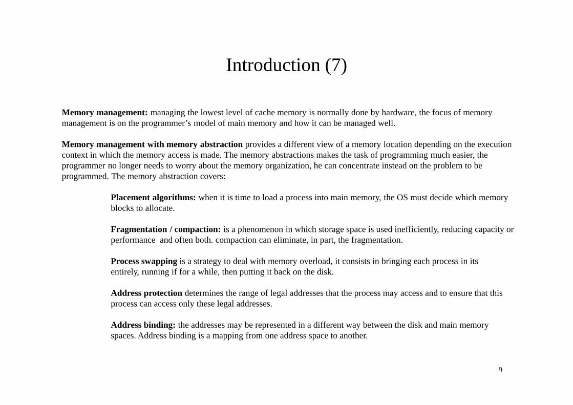
Memory management with memory abstraction provides a different view of a memory location depending on the execution context in which the memory access is made. The memory abstractions makes the task of programming much easier, the programmer no longer needs to worry about the memory organization, he can concentrate instead on the problem to be programmed. The memory abstraction covers:

Placement algorithms: when it is time to load a process into main memory, the OS must decide which memory blocks to allocate.

Fragmentation / compaction: is a phenomenon in which storage space is used inefficiently, reducing capacity or performance and often both. compaction can eliminate, in part, the fragmentation.

Process swapping is a strategy to deal with memory overload, it consists in bringing each process in its entirely, running if for a while, then putting it back on the disk.

Address protection determines the range of legal addresses that the process may access and to ensure that this process can access only these legal addresses.

Address binding: the addresses may be represented in a different way between the disk and main memory spaces. Address binding is a mapping from one address space to another.

10

Methods Partitioning Placement algorithms

Fragmentation / compaction

Swapping Address binding & protection

Layer

Fixed partitioningcontiguous / fixed /

complete

searching algorithms

yes / no

yes

no / yes (MMU) OS kernel

Memory managementwith bitmap

contiguous / dynamic /complete

yes / yesMemory managementwith linked lists

contiguous / dynamic / complete

Buddy memory allocation

contiguous / hybrid / complete

yes / no

Simple paging and segmentation

noncontiguous / dynamic / complete

yes / no yes (TLB)programs / services

Introduction (8)


1. Introduction








3.2. Segmentation

11

12




Layer


complete


yes / no

yes








yes / no




Partitioning and placement algorithms “Fixed partitioning”

13

Fixed partitioning: the simple scheme for managing available memory is to partition into regions with fixed boundaries. There are two alternatives for fixed partitioning, with equal-size or unequal-size partitions.

Size of partitions

Max loading size

Memory fragmentation

Degree of multi-

programming

Placement algorithms

equal-size partitions

M <M High High Single FIFO queue

unequal-size partitions

[M-N] with M<N

<N Medium Medium Single / multiple FIFO queue(s)

new processes

new processes

new processes

equal-size partitions unequal-size partitions, single queue unequal-size partitions, multiple queues

14




Layer


complete


yes / no

yes








yes / no




Partitioning and placement algorithms“Memory management with bitmaps”

15

Memory management with bitmaps: with a bitmap, memory is divided into allocation units as small as a few words and as large as several kilobytes. Corresponding to each allocation units is a bit in the bitmap, which is 0 if the unit is free and 1 if it is occupied (or vice versa).

A B C D E

0 5 8 14 18 20 26 29 32

e.g. a part of memory with five processes and three holes, with the corresponding bitmap.

0-7 1 1 1 1 1 0 0 0

8-15 1 1 1 1 1 1 1 1

16-23 1 1 0 0 1 1 1 1

24-32 1 1 1 1 1 0 0 0

The size of a the allocation unit is an important design issue:

- the smaller the allocation unit, the larger the bitmap. e.g. with an allocation unit of 4 bytes (32 bits), the bitmap will take 1/33 of the memory.

- if the allocation unit is chosen large, the bitmap will be smaller. However, appreciable memory may be wasted in the last unit of process due to the rounding effect.

Another problem is the placement algorithm. When it has been decided to bring k unit process into memory, we must search k consecutive 0 bits in the map, that is a slow operation.

Partitioning and placement algorithms“Memory management with linked lists” (1)

16

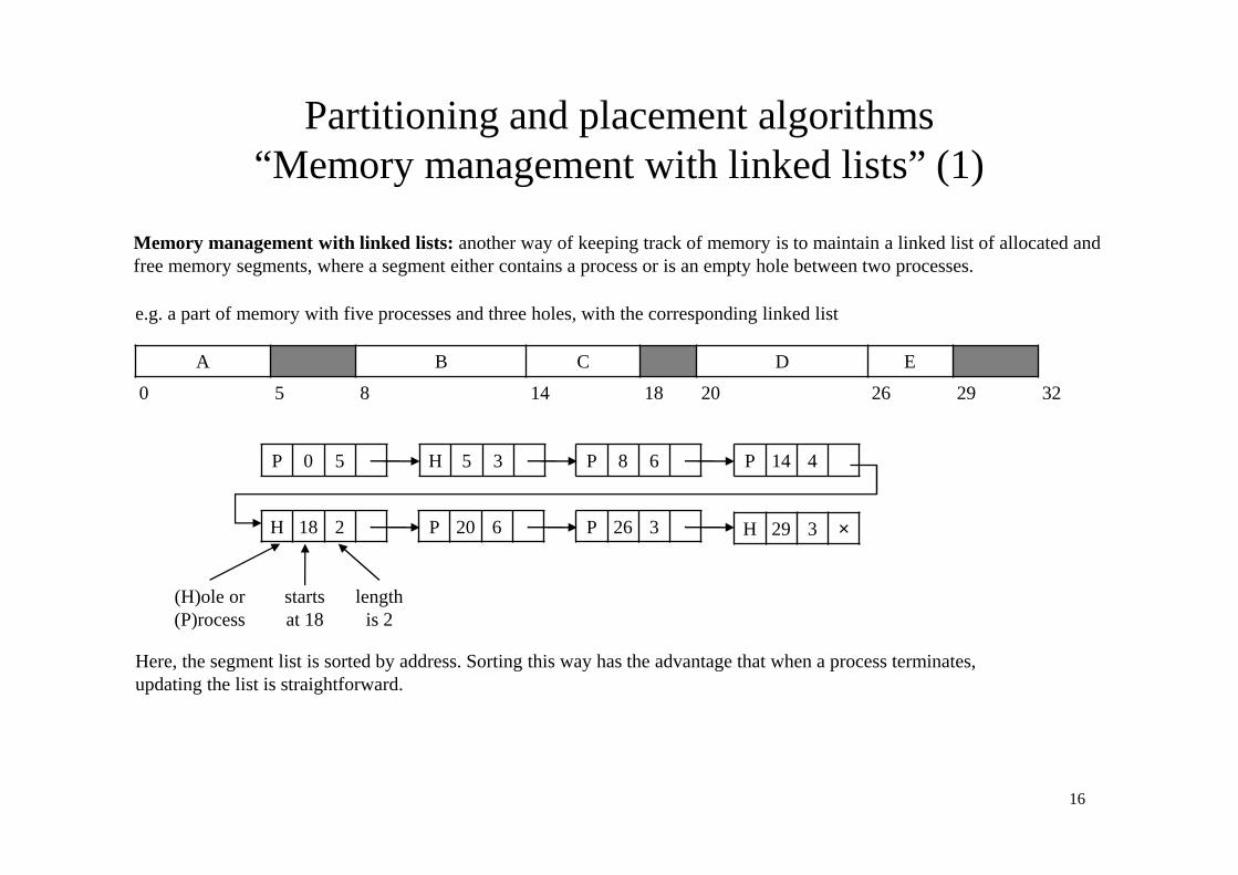
Memory management with linked lists: another way of keeping track of memory is to maintain a linked list of allocated and free memory segments, where a segment either contains a process or is an empty hole between two processes.

A B C D E

0 5 8 14 18 20 26 29 32

e.g. a part of memory with five processes and three holes, with the corresponding linked list

P 0 5 P 8 6H 5 3 P 14 4

H 18 2 P 20 6 P 26 3 H 29 3 ×

(H)ole or (P)rocess

starts at 18

length is 2

Here, the segment list is sorted by address. Sorting this way has the advantage that when a process terminates, updating the list is straightforward.


17


A terminating process has two neighbors (except when it is at the very top or bottom of the memory). These may be either processes or holes, leading to four combinations.

A X B

A X H

H X B

H X H

A H B

A H

H B

H

before X terminates after X terminates

becomes

H are holes, A, B and X processes

Since the process table slot for the terminating process will normally point to the list entry for the process itself, it may be more convenient to have the list as a double-linked list.


18


Several algorithms can be used to allocate memory for a created process.

Statistical analysis reveals that the first-fit algorithm is not only the simplest one but usually the best and fastest as well.

Algorithms Descriptions

first-fit It scans along the list of segments from beginning until it finds a hole that is big enough.

next-fit It works the same way as first fit, except that it keeps track of where it is whenever it finds a suitable hole.

best-fit It searches the entire list, from beginning to end, and takes the smallest hole that is adequate rather than breaking up a big hole that might be needed later.

worst-fit To get around the problem, one could think about worst fit, that is, always take the largest available hole.

quick-fit It maintains separate lists for some of the most common sizes requested, to speed up the best-fist.


19

Type Size (MB)

H 8

P4 …

H 12

P1 …

H 22

P3 …

H 18

P5 …

P2 …

H 8

P7 …

H 6

P6 …

H 14

P8 …

H 36


e.g. a memory with 8 processes (P1 to P8), P2 is the last allocated. What about P9 (16 MB) with the placement algorithms.

the last allocated block

initial state first fit best fitnext fit

Type Size (MB)

H 8

P4 …

H 12

P1 …

P9 16

H 6

P3 …

H 18

P5 …

P2 …

H 8

P7 …

H 6

P6 …

H 14

P8 …

H 36

Type Size (MB)

H 8

P4 …

H 12

P1 …

H 22

P3 …

P9 16

H 2

P5 …

P2 …

H 8

P7 …

H 6

P6 …

H 14

P8 …

H 36

Type Size (MB)

H 8

P4 …

H 12

P1 …

H 22

P3 …

H 18

P5 …

P2 …

H 8

P7 …

H 6

P6 …

H 14

P8 …

P9 16

H 20

20




Layer


complete


yes / no

yes








yes / no




Partitioning and placement algorithms“Buddy memory allocation” (1)

21

The Buddy memory allocation: fixed and dynamic partitioning schemes have drawbacks. A fixed partitioning limits the number of process and may use space inefficiently. The dynamic partitioning is more complex to maintain and includes the overhead of compaction. An interesting compromise is the Buddy memory allocation, employing an hybrid partitioning.

blocks in a buddy system, memory blocks of holes are available of size 2K, with L ≤ K ≤ U (L, U are the smallest and largest sizes blocks respectively).

init to begin, the entire space is treated as a single block hole of size 2K=U.

request at any time, the buddy system maintains a list of holes (unallocated blocks) of each size 2i:(1) a hole may be removed from the i+1 list by splitting it in half to create two buddies of size 2i in the i list. (2) whenever a pair of buddies on the i list becomes unallocated, they are removed from that list and coalesced into a single block on the i+1 list of size 2i+1. (3) presented a request for an allocation of size s such that 2i -1 ≤ s ≤ 2i, the following recursive algorithm applies.

get hole of size iif i equals U+1 or L-1

failureif the list i is empty

get hole of size i+1split hole into buddiesput buddies on the i list

take first hole on the i list

failure case

recursive search

access case


22


e.g. a 1MB memory with L=6 ≤ K ≤ U=10, considered blocks are 64K, 128K, 256K, 512K, 1MB.

1 MB block 1 MB

request A = 100K A=100K 128K 256K 512K

request B = 240 K A=100K 128K B=240K 512K

request C = 64 K A=100K C=64K 64K B=240K 512K

request D = 256K A=100K C=64K 64K B=240K D=256K 256K

release B A=100K C=64K 64K 256K D=256K 256K

release A 128K C=64K 64K 256K D=256K 256K

request E = 75K E=75K C=64K 64K 256K D=256K 256K

release C E=75K 128K 256K D=256K 256K

release E 512K D=256K 256K

release D 1MB


23


e.g. a 1MB memory with L=6 ≤ K ≤ U=10, considered blocks are 64K, 128K, 256K, 512K, 1MB.

release B A=100K C=64K 64K 256K D=256K 256K

1 MB

512 K

256 K

128 K

64 K

non-leaf node

leaf node for unallocated block

leaf node for allocated block


1. Introduction








3.2. Segmentation

24

25




Layer


complete


yes / no

yes








yes / no




Memory fragmentation and compaction (1)

26

External fragmentation: with dynamic partitioning, as processes are loaded and removed from memory, the free memory space could be broken into little pieces. This phenomenon is known as external fragmentation of memory.

e.g. Type Size (MB)

H 56

56

initial state

Type Size (MB)

P1 20

H 36

Total 56

F Rate 0

(a) P1 (20MB) loaded

Type Size (MB)

P1 20

P2 14

H 22

Total 56

F Rate 0

(b) P2 (14MB) loaded

Type Size (MB)

P1 20

P2 14

P3 18

H 4

Total 56

F Rate 0

(c) P3 (18MB) loaded

Type Size (MB)

P1 20

H 14

P3 18

H 4

Total 56

F Rate 0,22

(d) P2 leaves

Type Size (MB)

P1 20

P4 8

H 6

P3 18

H 4

Total 56

F Rate 0,4

(e) P4 (8MB) loaded

Type Size (MB)

H 20

P4 8

H 6

P3 18

H 4

Total 56

F Rate 0,33

(f) P1 leaves

Type Size (MB)

P1 14

H 6

P4 8

H 6

P3 18

H 4

Total 56

F Rate 0,62

(g) P5 (14MB) loaded

( )∑∀

∀−=

ii

ii

H

HRateF

max1

One way to compute fragmentation rate of memory F Rate is


27


50-percent rule: memory fragmentation depends of the exact sequence of incoming processes, the considered system and placement algorithms (e.g. first, next and best fit). Statistical analysis reveals that even with some optimization, given N allocated blocks 0,5N block will be lost to fragmentation. That is, one third of memory may be unusable. This property is known as the 50-percent rule. NN

N

5,01

5,0

+


28


Memory compaction: when internal fragmentation results in multiple holes in memory, it is possible to combine them all into one big one by moving all the processes downward as far as possible. This technique is knows as memory compaction. It requires lot of CPU time.

e.g. on a 1GB machine that can copy 4 bytes in 20 ns, it would take 5 s to compact all memory.


29

Internal fragmentation: memory allocated to a process may be larger than the request memory, two cases occur.

Track overhead: the general approach is to break the physical memory into fixed size blocks and allocate memory in units based on block size. The difference between these two numbers is internal fragmentation of memory.

e.g.

Type Size (bytes)

P1 …

H 16384

P2 …

Type Size (bytes)

P1 …

P3 16382

H 2

P2 …

P3 (16382 bytes)

initial state

Type Size (bytes)

P1 …

P3 16384

P2 …

P3 (16382 bytes)

case without allocation of blocks of fixed-size, a hole of size 2 bytes is

produced

case with allocation of blocks of fixed-size 256 bytes,

64 blocks are allocated to P3internal fragmentation is then

16384-16382 = 2 bytes


30

Internal fragmentation: memory allocated to a process may be larger than the request memory, two cases occur.

Extra memory allocation: when it is expected that the most processes will grow as they run, it is probably a good idea to allocate a little extra memory.

e.g. a process with two growing segments, a data segment to being used as a heap for variables that are dynamically allocated and released, and a stack segment for the local normal variables and return addresses. An arrangement is to place the stack at the top that is growing downward, and the data segment just beyond the program text that is growing upward.

A-Program

A-Data

A-stack

B-Program

B-Data

B-stack

Hole

room for grow

room for grow


1. Introduction








3.2. Segmentation

31

32




Layer


complete


yes / no

yes








yes / no




Process swapping (1)

33

Swapping is a strategy to deal with memory overload, it consists in bringing each process in its entirely, running if for a while, then putting it back on the disk.

e.g. a 88MB memory system, we consider the following events with swapping.

Type Size (MB)

P1 32

H 56

Total 88

(a) P1 (32MB) loaded

Type Size (MB)

P1 32

P2 16

H 40

Total 88

(b) P2 (16MB) loaded

Type Size (MB)

P1 32

P2 16

P3 32

H 8

Total 88

(c) P3 (32MB) loaded

(d) P1 swapped out from disk

(e) P4 (16MB) loaded

Type Size (MB)

H 32

P2 16

P3 32

H 8

Total 88

Type Size (MB)

P4 16

H 16

P2 16

P3 32

H 8

Total 88

(f) P2 (16MB) leaves

Type Size (MB)

P4 16

H 32

P3 32

H 8

Total 88

(g) P1 swapped in at a different

location

Type Size (MB)

P4 16

P1 32

P3 32

H 8

Total 88


34


Operating System in

RAM


swap in

Backing store

swap out

criterionswap out I/O blocked processes, huge memory processes, ready processes

with low-level priorities, etc.

swap in no ready process in the ready queue, processes in the ready suspend queue with priorities higher to the ones in the ready queue, processes for which the blocking event will occur soon, etc.

Mid-term scheduler

Mid-term scheduler removes processes from main memory (if full) and places them on secondary memory (such as a disk drive) and vice versa.

Backing store is a fast disk that must be large enough to accommodate copies of all memory images. The system maintains suspend queues consisting in all processes whose are on the backing store. The context switch time in such a swapping system is fairly high.


35


The context switch time in such a swapping system is fairly high.

e.g. a user process of 10 MB and backing store with a transfer rate of 40 MB.s-1

- The standard swap operation is 10/40 = ¼ s = 250 ms.- Assuming no head seeks are necessary, and a latency of 8 ms, the swap time is 258 ms.

- The total swap time (in and out) is then 516 ms.Operating System in

RAM


swap in

Backing store

swap out

Mid-term scheduler


1. Introduction








3.2. Segmentation

36

37




Layer


complete


yes / no

yes








yes / no




Loading, address binding and protection “Loading and address binding” (1)

38

module 1

module 2

module n

static library

…

linkerload

module

dynamic library

loader program

main memorydisk memory

address binding

Loading: the first step is to load a program into the main memory and to create a process image. Any program consists in compiled modules in an object-code form linked together or to library routines. The library routines can be incorporated into the program or referenced as a shared code to be call at the run time.

Address space is the set of addresses that a process can use to address memory. Each process has its own address space, independent of those belonging to other processes.

Address binding: addresses may be represented in different way between the disk and main memory spaces. Address binding is a mapping from one address space to another.


39

Loading mode Binding time

Absolute loading

At the programming time

At the compile or assembly time

Relocatable loading at the load time

Dynamic loading at the run time

module 1

module 2

module n

static library

…

linkerload

module

dynamic library

loader program

main memorydisk memory

address binding


40

Absolute loading: an absolute loader requires that a given load module always be loaded into the same location in main memory. Thus, in the load module presented to the loader, all address references must be specific to main memory addresses.

Binding time Function

programming time

All actual physical addresses are directly specified by the programmer in the program itself. … …

ADD 92

MOV 88

84

80

76

72

68

JMP 88 64

load module C

Operating System in

RAM

main memory

0

64

256

C96


41

… …

ADD

MOV X

JMP X

Module C at programming

… …

ADD 92

MOV 88

84

80

76

72

68

JMP 88 64

load module C after compilation

Operating System in

RAM

main memory

0

64

256

C96


compile or assembly time

The program contains symbolic address references, and these are converted to actual physical addresses by compiler or assembler.

Absolute loading: an absolute loader requires that a given load module always be loaded into the same location in main memory. Thus, in the load module presented to the loader, all address references must be specific to main memory addresses.


42

Relocatable loading: when many programs share a main memory, it may not desirable to decide ahead of time into which region of memory a particular module should be loaded. It is better to make that decision at load time, thus we need a load module that can be located anywhere in main memory.


load time The compiler or assembler produces relative addresses. The loader translates these to absolute addresses at the time of program loading.

The load module must include information about that tells the loader where the addresses references are. This set of information is prepared by the compiler and referred as the relocation directory.

… …

ADD

MOV Y+X

JMP X+Y X

module before to be loaded

… …

ADD 92

MOV 88

84

80

76

72

68

JMP 88 64

module when loaded with X=128

Operating System in

RAM

Main memory

0

128C

132


43

Dynamic runtime loading: to maximize memory utilization, we would like to be able to swap the process image back into different locations at different times, that involves to update the load module at every swap. The relocatable loaders cannot support this scheme. The alternative is to defer the calculation of the absolute address until it is actually needed at run time.


run time The loaded program retains relative addresses, these are converted dynamically to absolute addresses by processor hardware.

Logical address space is the set of all logical addresses generated by a program, in the range [0,max].

Relocation register: the value R in the relocation register is added to every logical address to obtain the corresponding physical address.

Physical address space: is the set of all physical addresses corresponding to the logical addresses, in the range [R+0,R+max].

Memory Management Unit (MMU): the run time mapping from logical to physical addresses is done by an hardware device called MMU.

CPU

14000main

memory

relocation register

+logical address“346”

physical address“14346”MMU

Loading, address binding and protection “Address protection” (1)

44

Address protection: we need to make sure that every process has a separate memory space. To do this, we need the ability to determine the range of legal addresses that the process may access and to ensure that the process can access only these legal addresses. Protection of memory space is accomplished by having a special CPU hardware.

Non-dynamic address protection (absolute and relocatable loading)

CPU

base register

main memory≥

base + limit registers

<yes

no

yes

no

trap to operating system, addressing error

Base register holds the smallest legal physical memory address.

Limit (or bound) register specifies the size of the range e.g. if the base register holds 300 040 and limit register is 120 900, then the program can legally access all addresses from 300 040 to 420 940.

physicaladdress

Loading, address binding and protection “Address protection” (2)

45

Address protection: we need to make sure that every process has a separate memory space. To do this, we need the ability to determine the range of legal addresses that the process may access and to ensure that the process can access only these legal addresses. Protection of memory space is accomplished by having a special CPU hardware.

Dynamic address protection (dynamic runtime loading)

CPU

limit register

main memory<

logicaladdress

relocation register

+yes

no

trap to operating system, addressing error

physicaladdress

MMU with protection

The protection must be tuned with the relocation register in the case of MMU.


1. Introduction








3.2. Segmentation

46

47




Layer


complete


yes / no

yes








yes / no




Simple paging and segmentation“Paging, basic method” (1)

48

Paging: is a memory-management scheme that permits the physical address space of a process to be noncontiguous. The basic method for implementing paging involves breaking logical memory into fixed-sized blocks called pages and breaking physical memory into blocks of the same size called frame. A page table contains the base address of each page in physical memory. When a process is to be executed, its pages are loaded into any available memory frames from the backing store.

p data

0 page 0

1 page 1

2 page 2

3 page 3

f data

0

1 page 0

2

3 page 2

4 page 1

5

6

7 page 3

logicaladdress space

physicaladdress space

page number

frame number p f

0 1

1 4

2 3

3 7

frame number

page number

page table


49


e.g. 4 processes are loaded in main memory using paging: A, C (4 pages), B (3 pages) and D (5 pages).

0

1

2

3

4

5

6

7

8

9

10

11

12

13

14

(t0) initial state

0 A.0

1 A.1

2 A.2

3 A.3

4

5

6

7

8

9

10

11

12

13

14

(t1) A loaded

0 A.0

1 A.1

2 A.2

3 A.3

4 B.0

5 B.1

6 B.2

7

8

9

10

11

12

13

14

(t2) B loaded

0 A.0

1 A.1

2 A.2

3 A.3

4 B.0

5 B.1

6 B.2

7 C.0

8 C.1

9 C.2

10 C.3

11

12

13

14

(t3) C loaded

0 A.0

1 A.1

2 A.2

3 A.3

4

5

6

7 C.0

8 C.1

9 C.2

10 C.3

11

12

13

14

(t4) B swapped out

0 A.0

1 A.1

2 A.2

3 A.3

4 D.0

5 D.1

6 D.2

7 C.0

8 C.1

9 C.2

10 C.3

11 D.3

12 D.4

13

14

(t5) D loaded

frame number


50


e.g. 4 processes are loaded in main memory using paging with A, C (4 pages), B (3 pages) and D (5 pages).

p f

0 0

1 1

2 2

3 3

page table A

0 A.0

1 A.1

2 A.2

3 A.3

4 D.0

5 D.1

6 D.2

7 C.0

8 C.1

9 C.2

10 C.3

11 D.3

12 D.4

13

14

p f

0 -

1 -

2 -

page table B

p f

0 7

1 8

2 9

3 10

page table C

p f

0 4

1 5

2 6

3 11

4 12

page table D

f

13

14

free frame list

(t5) D loadeddata structure

at t5


51

Shared pages: an advantage of paging is the possibility of sharing common code. This can appear with reentrant code (or pure code) that is a non-self-modifying code i.e. it never changes during execution.

e.g. consider a system that supports three users, each of whom executes a text editor. It the text editor consists of 150 KB ofcode and 50 KB of data space, we need 600 KB to support the three users. If the code is reentrant code, it can be shared as:

0

1 data 1

2 data3

3 editor 1

4 editor 2

5

6 editor 3

7 data 2

8

9 data 4

10

11

loadedp Data

0 editor 1

1 editor 2

2 editor 3

3 data 1

Process 1

page number

p f

0 3

1 4

2 6

3 1

frame number

p Data

0 editor 1

1 editor 2

2 editor 3

3 data 2

Process 2

page number

p f

0 3

1 4

2 6

3 7

frame number

p Data

0 editor 1

1 editor 2

2 editor 3

3 data 3

Process 3

page number

p f

0 3

1 4

2 6

3 2

frame number

p Data

0 editor 1

1 editor 2

2 editor 3

3 data 4

Process 4

page number

p f

0 3

1 4

2 6

3 9

frame number


52

Address binding: every address generated by the CPU is dived in two parts, a page number (p) and a page offset (d). The page number is used as index into the page table, and the page table contains the base address of each page in physical memory. This base address is combined with the page offset (d) to define the physical memory address that is sent to the memory unit.

The size of a page is typically a power of 2 that makes the translation of a logical address into a page number and page offset particularly easy e.g. if the size of logical address space is 2m, and a page size is 2n addressing units, then the high order m-nbits designates the page number. As a result, the addressing scheme is transparent to programmer, assembler and linker.

p d

page number (p) page offset (d)

m-n n

m

m number of bits to encode thelogical address

n number of bit to encode the page offset

m-n number of bits to encode the page number


53


CPU page (p) offset (d)

page table*

frame

page table

logical address

+

page table*

p

page table*+p

frame (f) offset (d)

f*

data page

Main memory

f*+d

d


54


e.g. a memory of 16 bytes with a page size of 4 bytes, consider the logical address 0101.

address p d data

0000

0

0 a

0001 1 b

0010 2 c

0011 3 d

0100

1

0 e

0101 1 f

0110 2 g

0111 3 h

1000

2

0 i

1001 1 j

1010 2 k

1011 3 l

1100

3

0 m

1101 1 n

1110 2 o

1111 3 p

logical address space

p f

0 1

1 3

2 0

3 2

page table address f d data

0000

0

0 i

0001 1 j

0010 2 k

0011 3 l

0100

1

0 a

0101 1 b

0110 2 c

0111 3 d

1000

2

0 m

1001 1 n

1010 2 o

1011 3 p

1100

3

0 e

1101 1 f

1110 2 g

1111 3 h

the logical address 0101 (page 1, offset 1)

corresponds to the physical address 1101 (frame 3, offset 1)

physical address space


55

Address protection: address (or memory) protection in a paged environment is accomplished by protection bits associated to each frame. Normally, these bits are kept in the page table.

r/w bit: defines a page to be read-write or read only; we can easily expand this approach to provide a finer level of protection by considering execute-only sate.


56

Address protection: address (or memory) protection in a paged environment is accomplished by protection bits associated to each frame. Normally, these bits are kept in the page table.

valid bit: when this bit is set to valid, the associated page in the process’s logical address space is thus a valid page. When the bit is set to invalid; the page is not in the process’s logical address space.

e.g. in a system with m=14 bits address space (0 to 16383), using a page size of 2 KB, then n=11, m-n=3 (i.e. 8 pages). We have a process P of size 10438 bytes.

p data

0 page 0

1 page 1

2 page 2

3 page 3

4 page 4

5 page 5

f data

0 page 4

1 page 0

2

3 page 2

4 page 1

5

6

7 page 3

8 page 5

logicaladdress space

physicaladdress space

p f vb

0 1 true

1 4 true

2 3 true

3 7 true

4 0 true

5 8 true

6 × false

7 × false

valid bit

page tableP

Accesses to addresses up to 12287 (6×211) are valid, only the addresses from 12288 to 16383 are not valid.

Because the program extends to the address 10468 only, any reference beyond that address is illegal. This problem results of the 2KB page size and reflects the internal fragmentation of paging.


57

Transaction look-aside buffer (TLB): in principle every binding from logical address space to physical address space using paging causes two physical memory accesses (1) to fetch the appropriate page table entry (2) to fetch the desired data. This will have the effect of doubling the memory access time. To overcome this problem, we use a special high speed cache for page table entries called Transaction look-aside buffer (TLB).

TLB is an associative high speed memory. Each entry in the TLB consists of two parts {key; value}.

When an item (i.e. a page number) is presented, it is compared with all the keyssimultaneously. This technique is referred as associative mapping. If item == key, the corresponding value (i.e. offset) is returned.

The search is fast and hardware, however, is expensive. Typically, the number of entries in a TLB is small e.g. 64 to 1024 entries.

CPU page offset

page frame

frame offset

TLB

page table

TLB hit

TLB miss

main memory

physical address

logical address

add / replacement


58

TLB hit: it occurs when the page number is in the TLB.

TLB miss: if the page number is not in the TLB, we add the page number and frame so that they will be found quickly on the next reference. If the TLB is already full of entries, OS must select one entry for replacement (LRU or FIFO policy, etc).

wired down: some TLBs allow entries to be wired down, meaning that they cannot be removed from the TLB.


CPU page offset

page frame

frame offset

TLB

page table

TLB hit

TLB miss

main memory

physical address

logical address

add / replacement


59

Entry in the TLB

Access page table

Update TLB

Start

CPU generates physical address

yes i.e. TLB hitno i.e. TLB miss

CPU checks the TLB

TLB hit: it occurs when the page number is in the TLB.

TLB miss: if the page number is not in the TLB, we add the page number and frame so that they will be found quickly on the next reference. If the TLB is already full of entries, OS must select one entry for replacement (LRU or FIFO policy, etc).

wired down: some TLBs allow entries to be wired down, meaning that they cannot be removed from the TLB.



1. Introduction








3.2. Segmentation

60

61




Layer


complete


yes / no

yes








yes / no




Simple paging and segmentation“Segmentation” (1)

62

One vs. separated address spaces: logical addressing discussed so far is one-dimensional because the logical addresses go from zero to some maximum. For many problems, having separate logical address space may be much more better.

e.g. a compiler has tables that are built up as compilation proceeds, and each of them grows continuously. In a one dimensional memory, these tables are allocated contiguous chunks of logical addresses. Consider what happens if a program has a much larger than usual number of variables; the chunk of address space allocated for a table may fill up.

Some approaches to deal with are:

(1) the compiler could simply issue a message saying that the compilation cannot continue.

(2) to play “Robin Hood”, tacking space from the tables with an excess of room and giving it to the tables with little room. This is a nuisance at best and a great deal of tedious, unrewarding work, at worst.

Symbol table

Source text

constants

Parse-tree

Call stack

free

Symbol table has bumped into the source text table

free

free


63

Segmentation is a memory management scheme that supports independent address spaces called segment.-Each segment consists in linear sequence of addresses, from 0 to some maximum (usually very large). -The length of each segment may be anything from 0 to the maximum allowed. -Different segments may have different lengths. -Segment lengths may change during execution. -With segments, a logical address consists of a two tuple <segment number, offset>.

e.g. a compiler has tables that are built up as compilation proceeds, and each of them grows continuously. Because each segment constitutes a separate address space, the different segments can grow independently without affecting each other.

symbol table

constants

Source text

Parse tree

Call stackSegment 1 Segment 2

Segment 3 Segment 4

Segment 5

Logical address space


64

Segmentation: is a memory management scheme that supports independent address spaces called segment.-Each segment consists in linear sequence of addresses, from 0 to some maximum (usually very large). -The length of each segment may be anything from 0 to the maximum allowed. -Different segments may have different lengths. -Segment lengths may change during execution. -With segments, a logical address consists of a two tuple <segment number, offset>.

CPU seg (s) offset (d)

seg table*

base

segment table

logical address

+

seg table*

s

seg table*+s

base (b) offset (d)

b*

data segment

Main memory

b*+ d

d


65

Combined paging and segmentation: both paging and segmentation have their strengths. In combined paging / segmentation system, the user’s address space is broken up into a number of segments, at the discretion of the programmer. Each segment is, in turn, broken up into a number of fixed-size page.

-From the programmer’s point of view, a logical address still consists of a segment number and a segment offset.-From the system’s point of view, the segment offset is viewed as a page number and page offset for a page within the specified segment.

CPU s d

seg page table*

page table*

seg page table

logical address

+

seg page table*sseg page table*+s

f d

data

page

Main memory

p

+ frame

page table

page table*

page table*+p

p

operating systems “memory...

Documents