operation and design of diabatic distillation...
TRANSCRIPT
General rights Copyright and moral rights for the publications made accessible in the public portal are retained by the authors and/or other copyright owners and it is a condition of accessing publications that users recognise and abide by the legal requirements associated with these rights.
• Users may download and print one copy of any publication from the public portal for the purpose of private study or research. • You may not further distribute the material or use it for any profit-making activity or commercial gain • You may freely distribute the URL identifying the publication in the public portal
If you believe that this document breaches copyright please contact us providing details, and we will remove access to the work immediately and investigate your claim.
Downloaded from orbit.dtu.dk on: Jul 08, 2018
Operation and Design of Diabatic Distillation Processes
Bisgaard, Thomas; Huusom, Jakob Kjøbsted; Abildskov, Jens; von Solms, Nicolas; Pilegaard, Kim
Publication date:2016
Document VersionPeer reviewed version
Link back to DTU Orbit
Citation (APA):Bisgaard, T., Huusom, J. K., Abildskov, J., von Solms, N., & Pilegaard, K. (2016). Operation and Design ofDiabatic Distillation Processes. Kgs. Lyngby: Technical University of Denmark (DTU).

PhD Thesis
OPERATION AND DESIGN OF
DIABATIC DISTILLATION
PROCESSES
THOMAS BISGAARD
2016-02-28

Technical University of Denmark
Anker Engelundsvej 1
Building 101A
DK-2800, Kgs. Lyngby
Denmark
CVR-nr. 30 06 09 46
Phone: (+45) 45 25 25 25
Email: [email protected]
www.dtu.dk
©2016-02-28 Thomas Bisgaard
Printed by GraphicCo
Preface
This thesis is submitted as a partial fulfilment of the requirements for obtaining a
Doctor of Philosophy (PhD) degree at the Technical University of Denmark. The
thesis presents the main research results obtained during a three year period be-
tween September 2012 to February 2016.
The PhD project was conducted at the Department of Chemical and Biochem-
ical Engineering (CAPEC-PROCESS) under the supervision of Associate Professor
Jakob Kjøbsted Huusom and Associate Professor Jens Abildskov as main super-
visors and Associate Professor Nicolas von Solms and Professor Kim Pilegaard as
co-supervisors. A part of the work was conducted in collaboration with Professor
Sigurd Skogestad at the Department of Chemical Engineering, Norwegian Univer-
sity of Science and Technology (NTNU), Norway.
As the author of this thesis, I sincerely hope that this work will be considered
as a significant contribution to the development of the field of diabatic distilla-
tion. Furthermore, I hope that the obtained results will seed and inspire future
researchers to contribute to the field and that the developed materials and method
will be found useful in the process.
I would like to thank the Technical University of Denmark for funding the
project. A significant influence on the work is the supervision. I would hereby
thank all my supervisors, in particular Jakob and Jens, for their valuable social
and professional support, guidance, motivation, and criticism of the work. Positive
contributions to the motivation by other sources during the PhD has been highly
appreciated. In particular, I would mention Professor Emeritus Sten Bay Jørgensen
for providing feedback and showing interest in the work. Finally, I would like to
thank all the colleagues in CAPEC-PROCESS for providing a friendly, supporting
and attractive working environment. Especially, my "office mates" have made every
day - spent in the office - brighter.
During the three year duration of the PhD, I was granted the opportunity to

ii
spend three of the months in Trondheim (Norway) as an external research stay un-
der the supervision of Professor Sigurd Skogestad. This research stay resulted in a
new approach to the project, which led to significant contributions. I am very grate-
ful for the support from Professor Sigurd Skogestad and the colleagues at NTNU.
I am grateful to have been sharing three months with the friendly and helpful col-
leagues at NTNU and I hope the contact will persist.
Thomas Bisgaard
Kgs. Lyngby, 2016

Summary
Diabatic operation of a distillation column implies that heat is exchanged in one
or more stages in the column. The most common way of realising diabatic opera-
tion is by internal heat integration resulting in a heat-integrated distillation column
(HIDiC). When operating the rectifying section at a higher pressure, a driving force
for transferring heat from the rectifying section to the stripping section is achieved.
As a result, the condenser and reboiler duties can be significantly reduced.
For two-product distillation, the HIDiC is a favourable alternative to the con-
ventional distillation column. Energy savings up to 83% are reported for the HIDiC
compared to the CDiC, while the reported economical savings are as high as 40%.
However, a simpler heat-integrated distillation column configuration exists, which
employs compression in order to obtain a direct heat integration between the top
vapour and the reboiler. This configuration is called the mechanical vapour recom-
pression column (MVRC). Energy and economic savings of similar magnitude as the
HIDiC are reported for the MVRC. Hence, it is important to develop methods and
tools for assisting the selection of the best distillation column configuration.
The contributions of this work can be divided in three parts. The first part in-
volves the identification of the preferred distillation column configuration (CDiC,
MVRC, or HIDiC) for a given mixture to be separated. Correlations between phys-
ical parameters, distillation column design variables, and preliminary feasibility
indicators are investigated through simulations studies. The simulation studies in-
clude case studies, where different mixtures are separated in different distillation
column configurations. The considered mixtures are industrially relevant and their
thermodynamic behaviours vary considerable from one another. The HIDiC was
found to be the preferred configuration in terms of operating expenditures for mix-
tures of normal boiling point differences below 10 K.
The second part involves the investigation of the technological feasibility of the

iv
HIDiC. The impact on the column capacity (required tray area, entrainment flood-
ing, weeping) of different column arrangements of the internal heat transfer is
investigated. Furthermore, the ability to achieve stable operation of a concentric
HIDiC is investigated by systematically designing a regulatory control layer and a
supervisory control layer. Stable operation, in terms of column capacity and set-
point tracking, is demonstrated by simulation.
The final part covers the developed simulation tools and methods. A new dis-
tillation column model is presented in a generic form such that all the considered
distillation column configurations can be described within the same model frame-
work. The following distillation column configurations are considered:
• The conventional distillation column (CDiC)
• The mechanical vapour recompression column (MVRC)
• The heat-integrated distillation column (HIDiC)
• The secondary reflux and vaporisation column (SRVC)
The generic nature of the modelling framework is favourable for benchmarking dis-
tillation column configurations. To further facilitate benchmarking of distillation
column configurations, a conceptual design algorithm was formulated, which sys-
tematically addresses the selection of the design variables. The conceptual design
of the heat-integrated distillation column configurations is challenging as a result
of the increased number of decision variables compared to the CDiC. Finally, the
model is implemented in Matlab and a database of the considered configurations,
case studies, pure component properties, and binary interaction parameters is es-
tablished.
Resumé
Diabatisk drift af en destillationskolonne indebærer, at varme udveksles på en eller
flere bunde i kolonnen. En udbredt metode til at realisere diabatisk operation er
ved brug af indre varmeveksling, hvilket resulterer i den varmeintegrerede destil-
lationskolonne (engelsk forkortelse: HIDiC). Ved at operere forstærkersektionem
ved et højere tryk, kan en temperaturdrivkraft opnås, således at en varmeovergang
fra forstærkersektionen til afdriversektionen kan realiseres. Dette resulterer i, at
den krævede mængde energi, som fjernes fra kondensatoren og tilføres i kedlen,
reduceres betydeligt.
For destillationskolonner med to produkter, anses HIDiC som et favorabelt al-
ternativ til den konventionelle destillationskolonne (engelsk forkortelse: CDiC).
Energibesparelser på op til 83 % er rapporteret for HIDiC’en sammenlignet med
en CDiC , mens de rapporterede økonomiske besparelser er op til 40 %. Imidler-
tid, eksisterer en enklere varmeintegreret destillationskolonnekonfiguration, som
udnytter kompression til at opnå en direkte varmeintegration mellem den øverste
damp og kedlen. Denne konfiguration kaldes den mekaniske dampgenkompres-
sionskolonne (engelsk forkortelse: MVRC). Energimæssige og økonomiske bespar-
elser af lignende størrelsesorden som for HIDiC’en er rapporteret for MVRC’eren.
Derfor er det vigtigt at udvikle værktøjer og metoder til at udvælge den mest favor-
able destillationskolonnekonfiguration.
Bidragene fra dette arbejde kan opdeles i tre dele. Den første del involverer
identificering af den foretrukne destillationskolonnekonfiguration (CDiC, MVRC,
or HIDiC) for en given blanding, der skal separeres. Sammenhænge mellem fy-
siske parametre, designvariable, og simple evalueringsindikatorer undersøges via
simuleringersstudier. Simuleringersstudierne omfatter casestudier, hvor forskellige
blandinger bliver udført i forskellige destillationskolonnekonfigurationer. De be-
tragtede blandinger er industrielt relevante og deres termodynamiske egenskaber

vi
afviger betragteligt fra hinanden. HIDiC’en har vist sig at være den foretrukne kon-
figuration, hvad angår driftsomkostninger, for blandinger med normalkogepunkts-
forskelle under 10 kelvin.
Den anden del omfatter en undersøgelse af den teknologiske gennemførlighed
af en HIDiC. Inflydelsen af valget af måden, hvorpå HIDiC kolonnen arrangeres,
på kolonnenkapaciteten undersøges. Dette dækker over undersøgelser af kravet til
bundareal, samt risiko for væskelækage og -oversvømmelse på bundene. Endvidere
er evnen til at opnå stabil drift undersøgt ved systematisk at designe et stabilis-
erende kontrollag efterfulgt af et tilsynsførende kontrollag. Stabil drift, hvad angår
kolonne kapacitet og setpunktsporing, demonstreres ved simulering.
Den sidste del dækker over de udviklede simuleringsværktøjer og -metoder. En
ny destillationskolonnemodel præsenteres i en generisk form, således at alle de
betragtede destillationskolonnekonfigurationer kan beskrives inden for de samme
modelrammer. De betragtede destillationskolonnekonfigurationer er:
• Den konventionelle destillationskolonne (CDiC)
• Den mekaniske dampgenkompressionskolonne (MVRC)
• Den varmeintegrerede destillationskolonne (HIDiC)
• Sekundær refluks og fordampningskolonne (SRVC)
På grund af den generiske karakter af modelleringsrammen, kan sammenligningsstudier
af destillationskolonnekonfigurationer fortages på systematisk og konsistent vis. For
yderligere at forenkle sammenlingingsstudier af destillationkolonnekonfigurationer
er en konceptuel designalgoritme formuleret, som leder til en systematisk bestem-
melse af designvariablene. Det konceptuelle design af varmeintegrerede destilla-
tionkolonnekonfigurationer er udfordrende som følge af det øgede antal af design-
variable sammenligning med CDiC’en. Endeligt, er en Matlab-implementering af
modellen, samt en database over de betragtede konfigurationer og separationer,
etableret.

Contents
Contents vii
1 Thesis Overview 1
1.1 Motivation . . . . . . . . . . . . . . . . . . . . . . . . . . . . . . . . . 2
1.2 Thesis Objective and Goals . . . . . . . . . . . . . . . . . . . . . . . . 4
1.3 Thesis Outline and Contributions . . . . . . . . . . . . . . . . . . . . 6
1.4 Publications . . . . . . . . . . . . . . . . . . . . . . . . . . . . . . . . 8
1.4.1 Journal Papers . . . . . . . . . . . . . . . . . . . . . . . . . . 8
1.4.2 Reviewed Conference Papers . . . . . . . . . . . . . . . . . . 8
1.4.3 Other Documentation . . . . . . . . . . . . . . . . . . . . . . 9
2 Heat-Integrated Distillation Overview 11
2.1 Introduction . . . . . . . . . . . . . . . . . . . . . . . . . . . . . . . . 12
2.2 Distillation Methods . . . . . . . . . . . . . . . . . . . . . . . . . . . 12
2.2.1 Conventional Distillation Column . . . . . . . . . . . . . . . . 12
2.2.2 Heat Pump-Assisted Distillation . . . . . . . . . . . . . . . . . 14
2.2.3 Diabatic Distillation . . . . . . . . . . . . . . . . . . . . . . . 15
2.2.4 Internal Heat-Integrated Distillation . . . . . . . . . . . . . . 17
2.2.5 Advanced Internal Heat-Integrated Distillation . . . . . . . . 18
2.2.6 Thermally Coupled Distillation Columns . . . . . . . . . . . . 21
2.2.7 Summary of Heat-integrated Distillation Methods . . . . . . . 21
2.3 The Heat-Integrated Distillation Column . . . . . . . . . . . . . . . . 22
2.3.1 Experimental Studies . . . . . . . . . . . . . . . . . . . . . . . 23
2.3.2 Dynamic Modelling . . . . . . . . . . . . . . . . . . . . . . . . 30
2.3.3 Conceptual Design . . . . . . . . . . . . . . . . . . . . . . . . 30
2.3.4 Equipment Design . . . . . . . . . . . . . . . . . . . . . . . . 34
2.3.4.1 Compressor . . . . . . . . . . . . . . . . . . . . . . . 35

viii Contents
2.3.4.2 Internal Heat Exchangers . . . . . . . . . . . . . . . 37
2.3.4.3 Column Internals . . . . . . . . . . . . . . . . . . . . 39
2.3.5 Benchmark Studies . . . . . . . . . . . . . . . . . . . . . . . . 41
2.3.6 Operation . . . . . . . . . . . . . . . . . . . . . . . . . . . . . 46
2.3.6.1 Start-up . . . . . . . . . . . . . . . . . . . . . . . . . 47
2.3.6.2 Dynamics . . . . . . . . . . . . . . . . . . . . . . . . 47
2.3.6.3 Controllability . . . . . . . . . . . . . . . . . . . . . 48
2.4 Research Areas . . . . . . . . . . . . . . . . . . . . . . . . . . . . . . 49
3 Distillation Column Model 53
3.1 Introduction . . . . . . . . . . . . . . . . . . . . . . . . . . . . . . . . 55
3.2 Conservation Equations . . . . . . . . . . . . . . . . . . . . . . . . . 56
3.2.1 Mixing Stage . . . . . . . . . . . . . . . . . . . . . . . . . . . 57
3.2.2 Non-mixing Stage . . . . . . . . . . . . . . . . . . . . . . . . 58
3.3 Constitutive Equations . . . . . . . . . . . . . . . . . . . . . . . . . . 61
3.3.1 Vapour-Liquid Equilibrium . . . . . . . . . . . . . . . . . . . . 61
3.3.2 State Functions . . . . . . . . . . . . . . . . . . . . . . . . . . 62
3.3.3 Miscellaneous Equations . . . . . . . . . . . . . . . . . . . . . 63
3.3.4 Internal Heat Transfer . . . . . . . . . . . . . . . . . . . . . . 64
3.3.5 Non-mixing Stage Relations . . . . . . . . . . . . . . . . . . . 65
3.3.6 Tray Hydraulics . . . . . . . . . . . . . . . . . . . . . . . . . . 66
3.4 Performance Indicators . . . . . . . . . . . . . . . . . . . . . . . . . . 69
3.4.1 Second-law Efficiency . . . . . . . . . . . . . . . . . . . . . . 69
3.4.2 Operating and Capital Expenditures . . . . . . . . . . . . . . 69
3.4.2.1 Column . . . . . . . . . . . . . . . . . . . . . . . . . 71
3.4.2.2 Internal Heat Transfer . . . . . . . . . . . . . . . . . 72
3.4.2.3 Condenser and Side Heat Exchangers . . . . . . . . 72
3.4.2.4 Reboiler and Side Heat Exchangers . . . . . . . . . . 73
3.4.2.5 Compressor . . . . . . . . . . . . . . . . . . . . . . . 74
3.4.3 Hydraulic Feasibility Indicator . . . . . . . . . . . . . . . . . . 74
3.5 Model Implementation . . . . . . . . . . . . . . . . . . . . . . . . . . 76
3.5.1 Configuration Parameters . . . . . . . . . . . . . . . . . . . . 78
3.5.2 Proposed Specifications . . . . . . . . . . . . . . . . . . . . . 78
3.5.3 Implementation . . . . . . . . . . . . . . . . . . . . . . . . . . 81
3.5.4 Static Model Solution Procedure . . . . . . . . . . . . . . . . 82
3.6 Example: Separation of Benzene/toluene . . . . . . . . . . . . . . . 82
3.7 Discussion . . . . . . . . . . . . . . . . . . . . . . . . . . . . . . . . . 84
3.7.1 Model Evaluation . . . . . . . . . . . . . . . . . . . . . . . . . 84

Contents ix
3.7.2 Internals Limitation . . . . . . . . . . . . . . . . . . . . . . . 86
3.7.3 Economic Models . . . . . . . . . . . . . . . . . . . . . . . . . 86
3.8 Conclusion . . . . . . . . . . . . . . . . . . . . . . . . . . . . . . . . 87
4 Conceptual Design 93
4.1 Introduction . . . . . . . . . . . . . . . . . . . . . . . . . . . . . . . . 95
4.1.1 Configuration Generalisation . . . . . . . . . . . . . . . . . . 95
4.1.2 Design Reservations . . . . . . . . . . . . . . . . . . . . . . . 95
4.2 Nomenclature . . . . . . . . . . . . . . . . . . . . . . . . . . . . . . . 98
4.2.1 Design Degrees of Freedom . . . . . . . . . . . . . . . . . . . 98
4.2.2 Pairs – Heat-integrated Stages . . . . . . . . . . . . . . . . . . 98
4.2.3 Indexing . . . . . . . . . . . . . . . . . . . . . . . . . . . . . . 99
4.3 Design Method Overview . . . . . . . . . . . . . . . . . . . . . . . . 99
4.4 Detailed Description of the Design Method . . . . . . . . . . . . . . . 101
4.4.1 Step 1: Problem formulation . . . . . . . . . . . . . . . . . . 102
4.4.2 Step 2: Conceptual CDiC design . . . . . . . . . . . . . . . . . 102
4.4.3 Step 3: Target and configure heat integration type . . . . . . 103
4.4.4 Step 4: Improve design . . . . . . . . . . . . . . . . . . . . . 104
4.4.5 Step 4a: Adjust A . . . . . . . . . . . . . . . . . . . . . . . . . 104
4.4.6 Step 4b: Adjust NT . . . . . . . . . . . . . . . . . . . . . . . . 106
4.4.7 Step 4c: Configure pairing . . . . . . . . . . . . . . . . . . . . 106
4.4.8 Step 5: Converge simulation w.r.t. purity specifications . . . . 106
4.4.9 Step 6: Satisfy minimum temperature driving force and vapour
flow rate specifications . . . . . . . . . . . . . . . . . . . . . . 106
4.4.10 Step 7: Calculate design objective (Fob j) . . . . . . . . . . . . 108
4.4.11 Step 8: ∆Fob j sensitive? . . . . . . . . . . . . . . . . . . . . . 108
4.5 Method Illustration . . . . . . . . . . . . . . . . . . . . . . . . . . . . 109
4.5.1 Separation of Benzene/toluene . . . . . . . . . . . . . . . . . 109
4.5.1.1 CDiC design . . . . . . . . . . . . . . . . . . . . . . 109
4.5.1.2 HIDiC Design . . . . . . . . . . . . . . . . . . . . . . 111
4.5.1.3 MVRC Design . . . . . . . . . . . . . . . . . . . . . . 113
4.5.1.4 SRVC Design . . . . . . . . . . . . . . . . . . . . . . 114
4.5.1.5 No Prior Configuration Specification . . . . . . . . . 114
4.5.2 Multicomponent Aromatic Separation . . . . . . . . . . . . . 115
4.6 Design Considerations and Discussion . . . . . . . . . . . . . . . . . 118
4.6.1 Stripping Section Pressure . . . . . . . . . . . . . . . . . . . . 118
4.6.2 Interplay Between Design Variables . . . . . . . . . . . . . . . 119
4.6.3 Constant Area Versus Constant Heat Duty . . . . . . . . . . . 120

x Contents
4.6.4 Method Benchmarking . . . . . . . . . . . . . . . . . . . . . . 121
4.7 Conclusion . . . . . . . . . . . . . . . . . . . . . . . . . . . . . . . . 122
5 Techno-Economic Feasibility Analysis 123
5.1 Introduction . . . . . . . . . . . . . . . . . . . . . . . . . . . . . . . . 125
5.2 Methods and Tools . . . . . . . . . . . . . . . . . . . . . . . . . . . . 125
5.2.1 Technical Feasibility . . . . . . . . . . . . . . . . . . . . . . . 125
5.2.1.1 Column Capacity . . . . . . . . . . . . . . . . . . . . 126
5.2.1.2 Feasibility of Compression . . . . . . . . . . . . . . . 127
5.2.2 Economic Feasibility . . . . . . . . . . . . . . . . . . . . . . . 128
5.2.3 Uncertainty and Sensitivity Analysis . . . . . . . . . . . . . . 129
5.2.3.1 Monte Carlo Simulation . . . . . . . . . . . . . . . . 129
5.2.3.2 Standardised Regression Coefficients . . . . . . . . . 130
5.2.3.3 Model Reduction . . . . . . . . . . . . . . . . . . . . 130
5.3 Feasibility Indicators – Observations and Expectations . . . . . . . . . 131
5.4 Case Studies . . . . . . . . . . . . . . . . . . . . . . . . . . . . . . . . 133
5.4.1 Benzene/toluene . . . . . . . . . . . . . . . . . . . . . . . . . 133
5.4.1.1 Conceptual Design . . . . . . . . . . . . . . . . . . . 133
5.4.1.2 Technical Feasibility . . . . . . . . . . . . . . . . . . 133
5.4.1.3 Configuration Benchmarking . . . . . . . . . . . . . 136
5.4.2 Propylene/propane . . . . . . . . . . . . . . . . . . . . . . . . 138
5.4.2.1 Conceptual Design . . . . . . . . . . . . . . . . . . . 138
5.4.2.2 Technical Feasibility . . . . . . . . . . . . . . . . . . 139
5.4.2.3 Configuration Benchmarking . . . . . . . . . . . . . 141
5.4.3 Summary . . . . . . . . . . . . . . . . . . . . . . . . . . . . . 143
5.5 Feasibility Analysis . . . . . . . . . . . . . . . . . . . . . . . . . . . . 143
5.5.1 Case Study Formulation . . . . . . . . . . . . . . . . . . . . . 143
5.5.2 Design Trends . . . . . . . . . . . . . . . . . . . . . . . . . . . 144
5.5.3 Quantification of OPEX Uncertainty . . . . . . . . . . . . . . . 150
5.5.4 Benchmarking . . . . . . . . . . . . . . . . . . . . . . . . . . 153
5.6 Conclusion . . . . . . . . . . . . . . . . . . . . . . . . . . . . . . . . 155
6 Stabilising Control 161
6.1 Introduction . . . . . . . . . . . . . . . . . . . . . . . . . . . . . . . . 163
6.1.1 Control Hierarchy . . . . . . . . . . . . . . . . . . . . . . . . 163
6.1.2 Economic Plantwide Control (Part 1) . . . . . . . . . . . . . . 164
6.1.3 Stabilising Control . . . . . . . . . . . . . . . . . . . . . . . . 166
6.1.4 Proportional-Integral Control . . . . . . . . . . . . . . . . . . 166
6.1.5 Case Study . . . . . . . . . . . . . . . . . . . . . . . . . . . . 167

Contents xi
6.2 Operation Analysis . . . . . . . . . . . . . . . . . . . . . . . . . . . . 167
6.2.1 Operational Degrees of Freedom . . . . . . . . . . . . . . . . 168
6.2.2 Identification of Secondary Controlled Variables (CV2) . . . . 170
6.3 Design of Regulatory Layer . . . . . . . . . . . . . . . . . . . . . . . 173
6.3.1 Liquid Holdup Control . . . . . . . . . . . . . . . . . . . . . . 173
6.3.2 Pressure and Temperature Control . . . . . . . . . . . . . . . 174
6.3.3 Liquid Pressure and Internals Hydraulics Control . . . . . . . 177
6.3.4 Recommendations and Discussion . . . . . . . . . . . . . . . 178
6.4 Dynamic Evaluations . . . . . . . . . . . . . . . . . . . . . . . . . . . 179
6.4.1 Tuning . . . . . . . . . . . . . . . . . . . . . . . . . . . . . . . 179
6.4.2 Regulatory Layer Performance . . . . . . . . . . . . . . . . . . 180
6.4.3 Open-loop Responses . . . . . . . . . . . . . . . . . . . . . . . 182
6.5 Conclusions . . . . . . . . . . . . . . . . . . . . . . . . . . . . . . . . 183
7 Optimising Control 187
7.1 Introduction . . . . . . . . . . . . . . . . . . . . . . . . . . . . . . . . 189
7.1.1 Economic Plant-wide Control (Part 2) . . . . . . . . . . . . . 189
7.1.2 Optimising Control . . . . . . . . . . . . . . . . . . . . . . . . 189
7.1.3 Case Study . . . . . . . . . . . . . . . . . . . . . . . . . . . . 190
7.2 Top-down Design . . . . . . . . . . . . . . . . . . . . . . . . . . . . . 190
7.2.1 Definition of Optimal Operation . . . . . . . . . . . . . . . . . 190
7.2.2 Optimal Operation Point . . . . . . . . . . . . . . . . . . . . . 192
7.2.3 Active Constraint Regions . . . . . . . . . . . . . . . . . . . . 194
7.3 Supervisory Control Layer Design . . . . . . . . . . . . . . . . . . . . 195
7.3.1 More Valuable Top Product . . . . . . . . . . . . . . . . . . . 196
7.3.2 More Valuable Bottom Product . . . . . . . . . . . . . . . . . 196
7.4 Dynamic Evaluation . . . . . . . . . . . . . . . . . . . . . . . . . . . 199
7.4.1 Tuning . . . . . . . . . . . . . . . . . . . . . . . . . . . . . . . 199
7.4.2 Evaluation . . . . . . . . . . . . . . . . . . . . . . . . . . . . . 199
7.4.2.1 Single Disturbance Scenarios . . . . . . . . . . . . . 199
7.4.2.2 Mixed Disturbance Scenario . . . . . . . . . . . . . . 203
7.5 Conclusion . . . . . . . . . . . . . . . . . . . . . . . . . . . . . . . . 203
8 Thesis Conclusions 205
9 Future Directions 207
Bibliography 209
A Model Impelementation Documentation 223

xii Contents
A.1 Model Hierarchy . . . . . . . . . . . . . . . . . . . . . . . . . . . . . 223
A.2 Database . . . . . . . . . . . . . . . . . . . . . . . . . . . . . . . . . . 223
A.3 Implementation . . . . . . . . . . . . . . . . . . . . . . . . . . . . . . 223
B Mathematical Derivations 227
B.1 State Functions . . . . . . . . . . . . . . . . . . . . . . . . . . . . . . 227
B.2 Derivatives Chain Rule Algebra . . . . . . . . . . . . . . . . . . . . . 228
B.3 Compressor Feasibility . . . . . . . . . . . . . . . . . . . . . . . . . . 229
B.4 Compression Ratio . . . . . . . . . . . . . . . . . . . . . . . . . . . . 230
C Supplementary Material for Economic Model 233
D Extended BP Method 235
E Design Method Comparison 241
E.1 Nominal Design . . . . . . . . . . . . . . . . . . . . . . . . . . . . . . 242
E.2 Ponchon-Savarit . . . . . . . . . . . . . . . . . . . . . . . . . . . . . 242
E.3 Extended Ponchon-Savarit . . . . . . . . . . . . . . . . . . . . . . . . 246
F Notation 251

Chapter1
Thesis Overview
This chapter contains a general overview of the PhD project with
emphasis on its contributions. A brief introduction outlining the
motivation, challenges and perspectives of diabatic distillation
is presented. The project goals and the overall structure of the
thesis document is provided here as well. Finally, dissemination
activities related to the project and the main achievements are
briefly outlined.

2 Chapter 1. Thesis Overview
1.1 Motivation
Multi-stage distillation has been known since the 16th century. Today, distillation
is the most widely used technique for separating chemical mixtures. In fact, it
is estimated that more than 40,000 columns are currently operating worldwide
[85] accounting for 40% of the energy consumed in the chemical industry. The
energy consumed by distillation in 1978 was estimated to be 1458 PJ distributed
among the different sectors shown in Figure 1.1. In particular, improvements in
the petrochemical sector will lead to significant energy reductions. Many of the
well-established industries have a reputation of being conservative and therefore, it
is believed that the data fairly represents modern distillation energy consumption.
Petro
leum
fuel
fracti
ons
Light
hydr
ocar
bons
Wate
r-oxy
gena
tedhy
droc
arbo
ns
Aromati
cs
Wate
r-ino
rgan
ics
Other
s
Misc
ellan
eous
0
200
400
600
800821
255
10768 55 37
115
Ener
gyco
nsum
ptio
n[ PJ
yr−
1]
Figure 1.1. Estimated total U.S. distillation energy consumption 1978 [105]. Thetotal energy consumption is 1458 PJyr−1.
Distillation offers a large number of advantages; it is usually the most econom-
ical method of separating liquid mixtures [162], it has a wide application range,
and it is a technologically mature process. The key disadvantages are the high en-
ergy input requirement and its low thermodynamic efficiency. Industrial distillation
columns operate at thermodynamic efficiencies in the range of 5-20% [26]. The

1.1. Motivation 3
low thermodynamic efficiency is related to the heat addition at a relative high tem-
perature in the bottom of the distillation column and energy removal at a relative
low temperature in the top of a column. As a consequence, conventional heat inte-
gration within a distillation column is limited to feed preheating using the sensible
heat of the bottoms product stream.
Improvements in distillation have been investigated since its industrial imple-
mentation. Particularly, the oil and energy crises during the 70’s contributed to a
significant interest in improved energy efficiency. In 1978 it was estimated that a
decrease of energy consumption of 10% in distillation would conserve the equiv-
alent of 100,000 barrels of oil per day [105]. To put things in perspective, the
US imported twice the amount of crude oil per month (approx. 200,000 barrels
of crude oil per month) during the same year [3]. The focus on effective energy
management is not only driven by economics. It is widely acknowledged that the
increasing CO2 emissions associated with energy consumption, are correlated with
the global climate change. Predictions foresee an increase in the average global
temperature of up to 6◦C by 2050 if current emission trends persist [65]. With all
industrial processes accounting for 5% of the global CO2 emissions in 2009 [65],
a strong motivation exists to improve current technologies in every sector within
the chemical industry. This includes distillation as it takes up 40% of the energy
consumption in the chemical industry.
Several attempts to save energy have been proposed. These can be divided
into the categories listed in Table 1.1. The improvements either involve changes
with impact on the separation process or changes without impact on the separation
process. These can further be divided in separation and energy efficiency-related
improvements. Examples of each category are listed. This thesis focuses on the en-
ergy related categories. Examples of energy efficiency-related improvements with
impact on the separation are intensified distillation configurations including the
heat-integrated distillation columns [94]. Examples of the efficiency-related im-
provements without impact on the separation are the heat pump assisted distillation
columns [34]. These configurations reflect types of heat integration for stand-alone
distillation columns and cover external and internal heat integration, corresponding
to vapour recompression and diabatic operation [43], respectively. Configurations,
containing either or both types of heat integration, typically require compression.
Electricity is invested in compression in order to reuse the latent heat removed
in the top of a column, which is otherwise discarded in conventional distillation
columns. Significant energy savings are reported for the heat-integrated distillation
configurations. Potentially, this can lead to reductions in operation costs, over-
coming the increased investment costs associated with additional heat exchange

4 Chapter 1. Thesis Overview
Table 1.1. Options and classification of energy conservation methods in distillationinspired by Mix et al. [105].
Without impact on the process With impact on the process
Separation effi-ciency
Energy efficiency Separation effi-ciency
Energy efficiency
• Controlretrofit (ad-just/updatetuning, struc-ture etc.)
• Tray internalsretrofit
• Insulation• Reboiler main-
tenance• Feed/product
heat exchange• heat pump
(vapour com-pression andvapour recom-pression)
• Side draw• Alternate tech-
niques (e.g.extractivedistillation)
• Thermal cou-pling (e.g.dividing wallcolumn)
• Intermediateheat exchang-ers
• Internal heatintegration(diabatisation)
equipment and compression. For example, energy savings up to 90% have been
demonstrated by simulation of the heat-integrated distillation column separating
propylene/propane [158]. An interesting catagory of separations that show a sig-
nificant potential for energy improvements are the close-boiling mixtures, typically
found in the petrochemical industry. This catagory includes the propylene/propane
separation. The separations of close-boiling mixtures are typically very energy de-
manding and requires tall distillation towers with large internal flow rates. Accord-
ing to Figure 1.1, 90% of the 255 PJ energy spent on separating light hydrocarbons
almost corresponds to a quarter of the brutto energy consumption of Denmark [2].
Hence, improvements in distillation in the light hydrocarbon industry appears to
have a potential for large energy savings.
1.2 Thesis Objective and Goals
Employing heat pump in distillation is a relatively old concept but its advantages
appears not to be fully exploited. Several options exist for intensified binary dis-
tillation [85] but the potentials among the different heat pump assisted distilla-
tion configurations are not fully understood. Extensive efforts have been made to
develop the diabatic distillation technology since the late 70’s. Despite demon-
strations of large energy savings and manageable operability of e.g. the internally
heat-integrated distillation column compared to the conventional distillation col-
umn, it has not yet been widely adopted by the industry. It is expected that this
is due to lack of mature methods for designing these more complex configurations

1.2. Thesis Objective and Goals 5
and the investment cost associated with additional equipment (the compressor).
These two factors constitute a significant psychological barrier for choosing such
configurations over the familiar conventional ones [87].
The aim of this PhD project is to shed light on the potential benefits of diabatic
operation and address some of the barriers for industrial application/acceptance of
diabatic distillation columns. There is a need for research and comparative studies
that can help to provide analysis of the pros and cons of novel and intensified dis-
tillation processes compared to conventional columns, while considering a broader
range of separations. These studies must address both static as well as dynamic
analysis. The following topics have been identified to comprise an important con-
tribution:
1. Modelling: Improvements in the modelling is an important task, since the use
of simplistic models can represent limitations. For example, in several pub-
lished models, pressure dynamics or sensible heat effects are often ignored.
Furthermore, it is important that models for conducting benchmark studies
of distillation column configurations are consistent (same level of detail, eco-
nomic parameters etc.).
2. Analysis and benchmarking: Consistent and systematic analysis of the po-
tential benefits of intensified distillation solutions are required. It is observed
that different means of analysis are reported in literature, which can lead
to bias towards certain configurations. Current studies report very differ-
ent figures for potential energy savings, which clearly constitutes a problem
in relations to achieving industrial acceptance. Few authors have addressed
this issue by proposing systematic evaluations. In addition, published case
studies of industrial relevance are limited to a quite narrow range of sepa-
rations. For example, benchmarking results of the separation of benzene/-
toluene are often reported. Furthermore, it is desired (if possible) to link
the desired distillation configurations to the physical properties of the compo-
nents in the mixture to be separated. This is an advantage in computer-aided
design frameworks as e.g. that of Jaksland et al. [72].
3. Conceptual design: The availability of simple, conceptual design methods
of heat-integrated distillation columns is limited compared to conventional
distillation columns. Furthermore, the realisation of the internals in the inter-
nally heat integrated columns still appears to be a challenge.
4. Operation: It is important to model and simulate a heat-integrated distil-
lation column as realistic as possible in order to conclude, whether it has

6 Chapter 1. Thesis Overview
acceptable operability for industrial application. Hence, all actuators must be
considered. Furthermore, it is important to devise a control structure, which
resembles that of the industrial practice.
1.3 Thesis Outline and Contributions
The thesis is divided into the following chapters listed with a short summary:
• Chapter 2 Heat-Integrated Distillation Overview: Literature overview of
heat-integrated distillation column configurations. A more detailed litera-
ture review is provided of the internally heat-integrated distillation column
(HIDiC), with the purpose of collecting, classifying, presenting, and discussing
the literature in order to identify perspectives and challenges of industrial im-
plementation. In contrast to the existing literature, the focus in the HIDiC
review is on the technical feasibility. Hence, the possibilities of physical re-
alisation in terms of achieving the required heat transfer areas, of choosing
appropriate column arrangements, and of obtaining stable operation are dis-
cussed. In particular, attention is paid to the implications of internal heat
transfer in distillation w.r.t. separation performance and heat transfer perfor-
mance is discussed in relation to conventional equipment.
• Chapter 3 Distillation Column Model: This chapter represents the core of
the work, in the sense it provides the modelling basis - the model framework
- which is used throughout the thesis. The implementation and the solution
procedure are presented end exemplified.
• Chapter 4 Conceptual Design: A simulation-based, conceptual design proce-
dure for heat-integrated distillation columns with compressors is presented.
The design method can be used to produce a conceptual design of any distilla-
tion configuration by iteratively, minimising the total annualised cost (TAC).
Depending on the required design, the method can provide a design for a
given configuration or a design of the configuration with the lowest TAC (with
no configurations specifications in advance). The method is explained step by
step and illustrated through examples. The presented method is a generalisa-
tion of the procedure for arriving at an optimal design, based on experience
from numerous rigorous simulations studies covering most possibilities of the
pairing of heat integrated stages.
• Chapter 5 Techno-Economic Feasibility Analysis: An extensive feasibility
study is presented, covering the separation of ten fundamentally different
1.3. Thesis Outline and Contributions 7
mixtures (nine binary and one multicomponent), carried out in four different
distillation column configurations. Links between mixture component physi-
cal properties, simple feasibility measures and the actual economic feasibili-
ties are established. Two case studies involving the separations of benzene/-
toluene and propylene/propane are highlighted. The presentations of the case
studies consist of illustrations of the basic features of the HIDiC, the concep-
tual designs, the technical feasibilities, and elaborate benchmarking studies.
In this regard, uncertainty analysis and sensitivity analysis are used on two
classes of mixtures (low/high normal boiling point differences) in order to
quantify the uncertainty of operating expenditure estimates and to identify
the more significant uncertain variables.
• Chapter 6 Stabilising Control: A regulatory control structure design is pro-
posed. Stable operation, in terms of setpoint tracking and avoiding entrain-
ment flooding and weeping, was achieved in the simulation of a concen-
tric HIDiC separating benzene/toluene. The necessity of including pressure
dynamics in modelling of the heat-integrated distillation columns is illus-
trated by benchmarking dynamic open-loop responses against a constant mo-
lar overflow-model.
• Chapter 7 Optimising Control: A supervisory control structure design is de-
vised based on the systematic, economic plant-wide control method by Lars-
son and Skogested [89]. Optimal operation of HIDiC is defined. The optimal
operating point is determined for a concentric HIDiC, separating a mixture
of benzene/toluene. The combined supervisory and regulatory control struc-
tures are evaluated by simulation and good performance is achieved w.r.t.
setpoint tracking of all controlled variables. Furthermore, good economic
performance is demonstrated for realistic disturbance scenarios.
• Appendices: In Appendix A, the model implementation documentation is
supplied, while mathematical derivations are collected in Appendix B. Ad-
ditional material for the economic model is provided in Appendix C. The
common model solution algorithm, known as the Wang-Henke boiling-point
method, is extended to cover heat-integrated distillation column configura-
tions. This extension is documented in Appendix D. Finally, Appendix E con-
tains the application examples of two existing graphical design methods.
Apart from the text, the thesis contains figures, tables and illustrations. The
illustrations are distinguished from the main text using shaded boxes. These il-
lustrations are used to elaborate on certain aspects in more detail and cover e.g.

8 Chapter 1. Thesis Overview
investigations of assumptions or analytical expressions, with the aim to provide an
order of magnitude perception. A consistent notation throughout the thesis is used
and listed in the very end (page 251).
1.4 Publications
All the scientific publications produced during the PhD work are listed in this section
according to journal articles, peer-reviewed conference publications, and additional
publications. Chapter references in boldface brackets are used to indicate which
material, the corresponding publications are based upon. Hence, this section can
be used as a reference work if more condensed descriptions are preferred. The
contributions are published unless otherwise stated.
1.4.1 Journal Papers
Ordered list of journal papers, starting from the most recent contribution:
• T. Bisgaard, J.K. Huusom, and J. Abildskov. Conceptual design of heat-integrated
distillation columns with compressors. 2016 (Chapter 4) (in preparation)
• T. Bisgaard, J.K. Huusom, and J. Abildskov. Modeling and analysis of conven-
tional and heat-integrated distillation columns. AIChE Journal, 61(12):4251–
4263, 2015 (Chapter 3)
• M. Mauricio-Iglesias, T. Bisgaard, H. Kristensen, K.V. Gernaey, J. Abildskov,
and J.K. Huusom. Pressure control in distillation columns: A model-based
analysis. Ind Eng Chem Res, 53(38):14776–14787, 2014 (Chapter 3)
1.4.2 Reviewed Conference Papers
Ordered list of reviewed conference papers, starting from the most recent contribu-
tion:
• T. Bisgaard, S. Skogestad, J.K. Huusom, and J. Abildskov. Optimal operation
and stabilising control of the concentric heat-integrated distillation column.
11th IFAC International Symposium on Dynamics and Control of Process Systems– Trondheim, Norway, 2016 (Chapter 6 and 7)
• T. Bisgaard, J.K. Huusom, and J. Abildskov. Impact on model uncertainty of
diabatization in distillation columns. Proceedings of Distillation and Absorp-tion, pages 909–914, 2014 (Chapter 5)
1.4. Publications 9
• K. Meyer, L. Ianniciello, J.E. Nielsen, T. Bisgaard, J.K. Huusom, and J. Abild-
skov. Hidic – design, sensitivity and graphical representation. Proceedings ofDistillation and Absorption, pages 727–732, 2014 (Chapter 4)
• T. Bisgaard, J.K. Huusom, and J. Abildskov. A modeling framework for con-
ventional and heat integrated distillation columns. 10th IFAC InternationalSymposium on Dynamics and Control of Process Systems – Mumbai, India, pages
373–378, 2013 (Chapter 3)
• T. Bisgaard, J.K. Huusom, and J. Abildskov. Dynamic effects of diabatization
in distillation columns. Computer-aided Chemical Engineering, 32:1015–1020,
2013 (Chapter 6)
• T. Bisgaard, J.K. Huusom, and J. Abildskov. Dynamic effects of diabatiza-
tion in distillation columns. Proceedings of the 10th European Workshop onAdvanced Control and Diagnostics (ACD 2012), 2012 (Chapter 6)
1.4.3 Other Documentation
An extensive Matlab library has been developed, consisting of databases of physical
parameters, simulation case studies, and models. More details are provided in
Appendix A.

Chapter2
Heat-Integrated Distillation Overview
This chapter contains an overview of different heat-integrated
distillation configurations proposed in literature. During the
overview, the concept of diabatic distillation is introduced.
The following section presents a literature review of the heat-
integrated distillation column. The focus is on its techno-
economic feasibility. Experimental experiences, reported in lit-
erature, are summarised and discussed in relation to the pos-
sibilities and the challenges of equipment for the realisation of
the HIDiC.

12 Chapter 2. Heat-Integrated Distillation Overview
2.1 Introduction
Section 2.2 (below) will provide a step-by-step introduction to the concepts of the
HIDiC. At the end of Section 2.2 some more recent configurations are presented
and discussed.
Elaborate overviews of heat-integrated distillation technologies exist in litera-
ture [111, 37, 73, 86, 100, 85, 87, 126]. The present HIDiC review (Section 2.3)
deviates from the existing reviews in the sense that it aims to combine all aspects
of technological feasibility and economic feasibility.
Here, technological feasibility covers the possibilities of
• obtaining a feasible conceptual design,
• realising the obtained conceptual design in physical equipment, and
• maintaining stable, continuous operation when subject to disturbances.
Economic feasibility is when an economic benefit of a heat-integrated distillation
configuration, compared to conventional distillation, can be reaped. Thus, the eco-
nomic basis for benchmark studies is examined. The economic basis involves design
variables (heat exchange areas), model parameters (overall heat transfer coeffi-
cient), and economic parameters (steam price, cooling water price, and electricity
price). Based on the findings in the HIDiC literature review, Section 2.4 presents
the identified areas of research, which are covered in this thesis.
2.2 Distillation Methods
Distillation is a physical, multiphase separation technique that exploits the differ-
ences in relative volatilities of components and the counter-current movement of
the contacting vapour and liquid phases. The most common industrial distillation
column configuration is the conventional distillation column (CDiC), which are de-
scribed below.
2.2.1 Conventional Distillation Column
A conventional distillation column (CDiC) consists of a vertical column tower, a re-
boiler and a condenser as illustrated in Figure 2.1. The most common configuration
has two product streams and one feed stream. Gravity transports liquid downwards
inside the column because of the vertical orientation of the column, while vapour
moves upwards due to pressure differences between the bottom and the top, ini-
tiated by the reboiler. At each vertical position, a part of the entering vapour is

2.2. Distillation Methods 13
condensed and mixed with the entering liquid and the present liquid (holdup),
while a liquid amount of similar magnitude is vaporised due to the added latent
heat from the condensation. To generate these flows, the CDiC is equipped with a
heat exchanger in the top (the condenser) and in the bottom (the reboiler). The
role of the condenser is to fully or partly condense the vapour leaving the column
in the top. A fraction of the condensed vapour is recycled to the top of the column
(the reflux). The reboiler generates vapour flow (i.e. pressure) in the bottom by
evaporation (boilup). The products of the distillation column (see Figure 2.1) are
typically a distillate in the top (A) that is rich in the most volatile component(s) and
a bottom product (B) that is rich in the least volatile component(s). The column
is divided in two column sections: The rectifying section, which is above the feed
location, and the stripping section, which is below the feed location. The column
itself (excluding the condenser and the reboiler) is thermally insulated from the
surroundings and is therefore considered adiabatic.
AB
A
B
AB
A
B
B
A
AB
AB
A
B
AB
A
B
B
A
AB
B
A
AB
A
B
ABC
A
C
B ABC
A
C
B
A
B
AB
LP
HP
HP
HPLPLP
ABC
A
C
B
AB
BC
LP
HP
MPABC
A
BLP
HP
MP
C
HP
AB
A
B
B
AB
LP
HP
A
A
AB LP
HP
B
A
ABHP
LP
B
Figure 2.1. Conventional distillation column (CDiC).
The internals of a distillation column consists either of trays, structured pack-
ing material or random packing material.The purpose of the internals is to facili-
tate efficient mass transfer between the contacting liquid and vapour phases. For
tray columns, a stage is identical to a tray when assuming equilibrium.For packed
columns, the theoretical stage is often translated into an equivalent column height
(HETP, height equivalent to theoretical plate). In modelling, liquid-vapour equilib-
rium is typically assumed on each stage and is thus also called a theoretical stage

14 Chapter 2. Heat-Integrated Distillation Overview
or an equilibrium stage.
Stand-alone heat integration in a CDiC is limited to feed preheating using the
bottoms stream, where only sensible heat can be recovered. In the following sec-
tions, different distillation column configurations are presented that are able to
overcome this limitation by employing compression. The radical idea of introduc-
ing new equipment in distillation (e.g. a compressor), can potentially revolutionise
the old and well-known unit operation of distillation.
2.2.2 Heat Pump-Assisted Distillation
The heat pump-assisted distillation column, which was introduced in the 1950’s
[34], received renewed interest during the oil and energy crises in the 1970’s as
significant energy savings can be obtained. The heat pump enables the absorption
of heat from a cold source and the rejection of heat at a higher temperature sink,
which can directly translate into the condenser as the cold energy source (due to
condensation) and the reboiler as the hot temperature sink (due to vaporisation).
The simplest distillation configuration employing this principle is called the vapour
compression column (VCC) shown in Figure 2.2(a). In this configuration, an appro-
priate working fluid acts as an energy carrier between the condenser and reboiler.
As shown, compression and throttling is required.
Alternatively, the top vapour can be used as the working fluid thereby resulting
in the configuration illustrated in Figure 2.2(b). This configuration is commonly
known as the mechanical vapour recompression column (MVRC). A review on heat
pump assisted distillation technologies is provided by Jana [74]. The MVRC cir-
cumvents the additional compression cycle by letting the compressor work directly
on the top vapour. As vapour recompression can be obtained by different means
[86], the term "mechanical" is used to differentiate from e.g. the thermal vapour
recompression column (TVRC). In the TVRC, the required work for compression is
provided by a steam ejector thus limiting its application to systems with water pro-
duced as the distillate. The TVRC is not considered in this work. Both the VCC and
the MVRC can be classified as externally heat integrated distillation columns since
the heat exchange takes place outside the conventional distillation equipment. A
significant advantage of both the VCC and the MVRC is that the heat pump has no
impact on the separation. Therefore, such configurations appears to be very desired
in new applications as well as retrofitting, as they constitute a minimal technical risk
[127]. Furthermore, heat pump-assisted distillation has good operability as proven
by both simulation [107, 134, 135, 78] and experimentally [6, 90]. Furthermore,
significant economic and energy savings are reported [44, 127, 128, 30, 8, 32]. In
fact, it has already been successfully applied in the industry in the productions of 1-

2.2. Distillation Methods 15
AB
A
B
AB
A
B
B
A
AB
AB
A
B
AB
A
B
B
A
AB
B
A
AB
A
B
ABC
A
C
B ABC
A
C
B
A
B
AB
LP
HP
HP
HPLPLP
ABC
A
C
B
AB
BC
LP
HP
MPABC
A
BLP
HP
MP
C
HP
AB
A
B
B
AB
LP
HP
A
A
AB LP
HP
B
A
ABHP
LP
B
(a) Vapour Compression Column (VCC).
AB
A
B
AB
A
B
B
A
AB
AB
A
B
AB
A
B
B
A
AB
B
A
AB
A
B
ABC
A
C
B ABC
A
C
B
A
B
AB
LP
HP
HP
HPLPLP
ABC
A
C
B
AB
BC
LP
HP
MPABC
A
BLP
HP
MP
C
HP
AB
A
B
B
AB
LP
HP
A
A
AB LP
HP
B
A
ABHP
LP
B
(b) Mechanical Vapour RecompressionColumn (MVRC).
Figure 2.2. Externally heat-integrated distillation columns.
butene, chlorobenzene, ethanol, isopropanol and more [49]. Table 2.1 summarises
some feasibility studies from the open literature. The table clearly illustrates the
large savings compared to conventional distillation for a range of separations. It
also illustrates the dependency of the conclusions on the economic models. For
instance, separating the benzene/toluene in an MVRC is economically feasible ac-
cording to one study [51] but economically infeasible according to another study
[139]. However, the overall trend suggests that heat pump-assisted distillation is an
attractive alternative to conventional distillation as an economic benefit is achieved
for most reported separations.
2.2.3 Diabatic Distillation
In most cases, the column shell in conventional distillation is thermally insulated
causing adiabatic operation. If, instead, heat transfer is taking place at two or more
locations in the column (e.g. in the column trays), the column is said to be diabatic.
A general representation of a diabatic distillation column is given in Figure 2.3(a).
The distillation column with sequential heat exchangers (DSHE) is an exam-
ple of a diabatic distillation column (Figure 2.3(b)). In this configuration, heat is

16 Chapter 2. Heat-Integrated Distillation Overview
Table 2.1. Reported energy and economic savings of the mechanical vapour recom-pression column. The energy and economic savings are reported with reference to aCDiC performing the same separation; positive savings are in favour of the MVRC.Electrical energy is weighted by a factor of three for estimating the total energyconsumption in the HIDiC.
System Savings Reference
Energy Economy
BinaryAcetic acid/acetic anhydride 48% - [22]Propylene-propane - 21% [125]
- 44.1% [139]Benzene/fluoro-benzene - 54% [51]Benzene/n-heptane 66% 42% [51]Benzene/toluene - 17% [51]
- -24.9% [139]Benzene/chloro-benzene - 0% [51]Ethanol/water 67% 36% [51]Ethylbenzene/styrene 74% 69% [30]Methanol/water 50% 3.1% [141]
MulticomponentStyrene/benzene/toluene/ethylbenzene 79% 39% [51]Ethylbenzene/xylenes blend 62% 56% [30]Xylene blend 24% 47% [8]
removed in the rectifying section by letting a cold stream pass the inside of the col-
umn, thereby acting as an energy sink. As this stream is introduced in the top and
removed at a lower location the temperature can reach a higher value than what
can be obtained from a condenser. The stages in the rectifying sections can thus be
considered as sequential heat exchangers. In the same manner, a heating stream is
introduced in the bottom of the column and is extracted at a higher location.
This configuration has been studied as a means of improving the thermodynamic
efficiency of a distillation column by various authors [43, 77, 144]. Furthermore,
the concept of diabatic distillation has been proven experimentally by de Koeijer
and Rivero [25]. For a diabatic distillation column, a reduction in exergy loss of
39% can be obtained, meaning that the degradation of the energy quality is re-
duced compared to conventional distillation. Reports on economic savings have
not been encountered in the literature. This is likely due to the fact that no direct
benefits (i.e. energy requirement reductions) are achieved. Instead, the streams for
removing/adding energy in the condenser/reboiler become more potent for heat
integration, which can not easily be quantified in terms of economic improvements.

2.2. Distillation Methods 17
AB
A
B
AB
A
B
B
A
AB
AB
A
B
AB
A
B
B
A
AB
B
A
AB
A
B
ABC
A
C
B ABC
A
C
B
A
B
AB
LP
HP
HP
HPLPLP
ABC
A
C
B
AB
BC
LP
HP
MPABC
A
BLP
HP
MP
C
HP
AB
A
B
B
AB
LP
HP
A
A
AB LP
HP
B
A
ABHP
LP
B
(a) General diabatic distilla-tion column.
AB
A
B
AB
A
B
B
A
AB
AB
A
B
AB
A
B
B
A
AB
B
A
AB
A
B
ABC
A
C
B ABC
A
C
B
A
B
AB
LP
HP
HP
HPLPLP
ABC
A
C
B
AB
BC
LP
HP
MPABC
A
BLP
HP
MP
C
HP
AB
A
B
B
AB
LP
HP
A
A
AB LP
HP
B
A
ABHP
LP
B
(b) Distillation column withsequential heat exchangers(DSHE).
Figure 2.3. Diabatic distillation columns.
2.2.4 Internal Heat-Integrated Distillation
The principles of heat pump-assisted distillation can be used for enabling diabatic
operation in such a way that the rectifying section acts as a heat source and the
stripping section acts as a heat sink. Hence, the rectifying section must be operated
at a higher pressure in order to achieve the necessary temperature driving forces
among the heat-integrated stages. The two column sections are physically sepa-
rated (i.e. the rectifying section is not necessarily on top of the stripping section)
and a compressor is connected to the vapour leaving the stripping section, i.e. from
the feed stage. In accordance with the differences in pressures between the column
sections, a throttling valve is connected to the liquid stream leaving the rectifying
section. The obtained configuration is commonly referred to as the heat-integrated
distillation column (HIDiC) but was originally introduced along with the concept of
secondary reflux and vaporisation by Mah et al. [94]. The HIDiC is also referred to
as the internal thermally coupled distillation column by some authors [92] but the
term "thermal coupling" is commonly associated with the principle of the Petluyk
arrangement discussed in Section 2.2.6. In Figure 2.4(a), a conceptual representa-
tion of the HIDiC is presented. The variant of the HIDiC, where feed preheating is
used such that reboiler and condenser duties are avoided, is often called the ideal
18 Chapter 2. Heat-Integrated Distillation Overview
HIDiC (i-HIDiC) [73]. More recently, the term HIDiC is used to describe both in-
ternally heat integrated (diabatic) columns and columns, which have external heat
exchangers for realising heat integration between the column sections.
Additional energy can be recovered by using vapour recompression of the top
vapour in the HIDiC. This column was introduced along with the HIDiC by Mah
and Fitzmorris [31]. As the HIDiC abbreviation is fairly well established, the name
secondary reflux and vaporisation column (SRVC) will be used for a HIDiC hav-
ing condenser/reboiler heat integration using an additional compressor on the top
vapour. The SRVC is illustrated in Figure 2.4(b). Later, Mane et al. [98] considered
a configuration, which is conceptually identical to the SRVC. However, Mane et al.
used the name Intensified HIDiC.
The HIDiC is an intensified distillation column [5], which represent a radical,
stand-alone way of carrying out heat integration. Because of the promising fea-
tures of the HIDiC, extensive efforts have been made to develop this technology
during the past 15 years, both theoretically and experimentally. A more elaborate
description of the HIDiC is provided in Section 2.3.
2.2.5 Advanced Internal Heat-Integrated Distillation
Jana [73] provides an overview of applications of advanced distillation techniques
transferred to the HIDiC. Pressure-swing distillation is an apparent application of in-
ternal heat integration because two different column pressures already exist. How-
ever, two distillation columns are required rather than two column sections. Fol-
lowing the concepts of the HIDiC by choosing a high pressure rectifying section
as heat source and a low pressure stripping section as heat sink, the two config-
urations in Figure 2.5 are obtained for the two cases: (a) for a minimum-boiling
azeotropic mixture and (b) for a maximum-boiling azeotropic mixture [62]. Huang
et al. [62] provides a framework for designing the heat-integrated pressure swing
distillation columns and found for the separation of acetonitrile/water that up to
15% operating cost reductions and 14% capital cost reductions could be achieved
compared to a conventional sequence. However, it was concluded that this rectify-
ing/stripping section type heat integration fails to compete with the condenser/re-
boiler (multi-effect) type heat integration for the considered separation [62]. The
internally heat-integrated pressure-swing distillation columns arrangement is a spe-
cial case of the arrangement, referred to as the heat-integrated double distillation
columns (HIDDiC). The HIDDiC provides an alternative to a multi-effect distilla-
tion sequence for separations with more than two product splits (conceptually in-
cludes water/ethanol/azeotropic ethanol). The HIDDiC has been studied with the
heat integration of entire column sections [82] and with few heat-integrated stages

2.2. Distillation Methods 19
AB
A
B
AB
A
B
B
A
AB
AB
A
B
AB
A
B
B
A
AB
B
A
AB
A
B
ABC
A
C
B ABC
A
C
B
A
B
AB
LP
HP
HP
HPLPLP
ABC
A
C
B
AB
BC
LP
HP
MPABC
A
BLP
HP
MP
C
HP
AB
A
B
B
AB
LP
HP
A
A
AB LP
HP
B
A
ABHP
LP
B
(a) The Heat-Integrated DistillationColumn (HIDiC).
AB
A
B
AB
A
B
B
A
AB
AB
A
B
AB
A
B
B
A
AB
B
A
AB
A
B
ABC
A
C
B ABC
A
C
B
A
B
AB
LP
HP
HP
HPLPLP
ABC
A
C
B
AB
BC
LP
HP
MPABC
A
BLP
HP
MP
C
HP
AB
A
B
B
AB
LP
HP
A
A
AB LP
HP
B
A
ABHP
LP
B
(b) Secondary reflux and vaporisation Col-umn (SRVC).
Figure 2.4. Internally heat-integrated distillation columns. LP is the low-pressuresection and HP is the high-pressure section.
[167, 172, 59]. However, the benefit over a conventional multi-effect distillation
column arrangement has not been fully demonstrated. Furthermore, it is important
to note that the HIDDiC can potentially be operated without a compressor [82],
which is also the case for a multi-effect distillation sequence. Multi-effect distil-
lation denotes a distillation sequence, in which the columns operate at different
pressure such that e.g. condenser/reboiler type heat integration can be realised.
A more unconventional approach was adopted by Mulia-Soto et al. [108] and
Ponce et al. [131], where the entire distillation columns in a pressure-swing se-
quence were heat integrated. For the ethanol/water separation this leads to the
arrangement illustrated in Figure 2.5(c), which is referred to as an internally heat-
integrated pressure swing distillation process (IHIPSD). It was shown that by in-

20 Chapter 2. Heat-Integrated Distillation Overview
vesting 0.28 MW, the total reboiler duty could be reduced from 6.33 MW from a
conventional sequence to 4.30 MW for the IHIPSD. Condenser/reboiler type heat
integration was not considered in the mentioned studies [108, 131]. The study by
Mulia-Soto was later questioned [143], as reproducing the ethanol/water separa-
tion in conventional equipment was deemed extremely difficult. The separation of
ethanol/water, in particular, suffers from relatively low sensitivity of the azeotropic
composition to pressure. In the case of low pressure sensitivity, pressure swing dis-
tillation becomes practically impossible as the internal flow rates varies significantly
with small changes in product purities.
AB
A
B
AB
A
B
B
A
AB
AB
A
B
AB
A
B
B
A
AB
B
A
AB
A
B
ABC
A
C
B ABC
A
C
B
A
B
AB
LP
HP
HP
HPLPLP
ABC
A
C
B
AB
BC
LP
HP
MPABC
A
BLP
HP
MP
C
HP
AB
A
B
B
AB
LP
HP
A
A
AB LP
HP
B
A
ABHP
LP
B
(a) Internally Heat-Integrated Pressure-swing Distillation Column separatingminimum-boiling azeotrope [62].
AB
A
B
AB
A
B
B
A
AB
AB
A
B
AB
A
B
B
A
AB
B
A
AB
A
B
ABC
A
C
B ABC
A
C
B
A
B
AB
LP
HP
HP
HPLPLP
ABC
A
C
B
AB
BC
LP
HP
MPABC
A
BLP
HP
MP
C
HP
AB
A
B
B
AB
LP
HP
A
A
AB LP
HP
B
A
ABHP
LP
B
(b) Internally Heat-Integrated Pressure-swing Distillation Column separatingmaximum-boiling azeotrope [62].
AB
A
B
AB
A
B
B
A
AB
AB
A
B
AB
A
B
B
A
AB
B
A
AB
A
B
ABC
A
C
B ABC
A
C
B
A
B
AB
LP
HP
HP
HPLPLP
ABC
A
C
B
AB
BC
LP
HP
MPABC
A
BLP
HP
MP
C
HP
AB
A
B
B
AB
LP
HP
A
A
AB LP
HP
B
A
ABHP
LP
B(c) Internally Heat-IntegratedPressure-swing Distillation Col-umn (IHIPSDC) for separatingethanol/water [108].
Figure 2.5. Advanced internally heat-integrated distillation columns. LP is thelow-pressure section/column and HP is the high-pressure section/column.

2.2. Distillation Methods 21
2.2.6 Thermally Coupled Distillation Columns
Based on the patent by Brugma [18], Petlyuk et al. [129] introduced thermal cou-
pling in a distillation with a prefractionation column as illustrated in Figure 2.6(a).
By supplying the reflux and boil-up flows in the prefractionation column by directly
taking fractions of the internal vapour and liquid flows from the main column,
significant energy savings can be obtained for multicomponent separations. As a
result, an intensified arrangement was achieved called the Petlyuk arrangement. A
ternary distillation process is illustrated in Figure 2.6. A thermodynamically equiv-
alent configuration was filed as a patent [169] in 1949, in which both prefraction-
ation and distillation takes place in the same column shell (Figure 2.6(b)). This
configuration is known as the dividing wall column (DWC). In 1985 (35 years af-
ter its introduction [169]), the DWC was introduced in an industrial application by
BASF [126]. Since then, it has been industrially recognised as a common separation
technique of multicomponent mixtures.
AB
A
B
AB
A
B
B
A
AB
AB
A
B
AB
A
B
B
A
AB
B
A
AB
A
B
ABC
A
C
B ABC
A
C
B
A
B
AB
LP
HP
HP
HPLPLP
ABC
A
C
B
AB
BC
LP
HP
MPABC
A
BLP
HP
MP
C
HP
AB
A
B
B
AB
LP
HP
A
A
AB LP
HP
B
A
ABHP
LP
B
(a) Petlyuk configuration.
AB
A
B
AB
A
B
B
A
AB
AB
A
B
AB
A
B
B
A
AB
B
A
AB
A
B
ABC
A
C
B ABC
A
C
B
A
B
AB
LP
HP
HP
HPLPLP
ABC
A
C
B
AB
BC
LP
HP
MPABC
A
BLP
HP
MP
C
HP
AB
A
B
B
AB
LP
HP
A
A
AB LP
HP
B
A
ABHP
LP
B
(b) Dividing Wall Column (DWC).
Figure 2.6. Thermally coupled distillation columns.
2.2.7 Summary of Heat-integrated Distillation Methods
The previous sections only illustrate a handful of the many possibilities for intensi-
fying distillation. It is important, as a chemical plant design engineer, to be able to
identify the best distillation column configuration among the alternatives. Hence,
22 Chapter 2. Heat-Integrated Distillation Overview
it is important to investigate the feasibility of all alternatives when designing dis-
tillation units for chemical and biochemical plants. Kiss et al. [86] systematically
addressed this investigation for a wider range of configurations and proposed a
flow chart for selecting an appropriate distillation configuration for a given class
of separation. In the case of binary distillation, four distinct configurations were
covered in this chapter; the CDiC, the MVRC, the HIDiC, and the SRVC. According
to Kiss et al. [86], the HIDiC or the MVRC are among the preferred choices if (i) it
is a binary distillation, (ii) water is not a top product (distillate), and (iii) separa-
tion is above atmospheric pressure. In terms of separation involving more than two
product splits, i.e. multicomponent separations, the DWC or multi-effect distillation
sequences are typically the preferred option [86].
This issue of linking the feed mixture to the preferred distillation column con-
figuration has been the topic of various studies [51, 142, 155, 47]. These studies
conclude that the economic advantage of either configuration is a complex function
of mixture identity, whereas correlations between optimality and relative volatil-
ity have been shown for ideal mixtures. In particular, the study by Shenvi et al.
[142] concluded that the efficacy of the HIDiC can not be solely decided, based on
the feed and product specification, and pointed out that the shape of the column
temperature profile is the dominant factor. However, no direct and simple guide-
lines of selecting a configuration among the binary distillation techniques (e.g. the
MVRC and the HIDiC) have been encountered in literature. Hence, there is still a
need for systematically mapping the choice of superior configuration w.r.t. selected
performance criteria.
2.3 The Heat-Integrated Distillation Column
The heat-integrated distillation column (HIDiC) has a great potential as a stand-
alone distillation solution, due to following benefits:
• It provides reuse of otherwise wasted latent heat in the CDiC (like the MVRC)
but requires a lower compression ratio than that of the MVRC [94].
• The equipment size can potentially be reduced as one of the column sections
contains a denser, high-pressure vapour. Furthermore, a concentric arrange-
ment [45] can realise the HIDiC within one column shell.
• A compressor is a more reliable energy source/sink than steam/cooling water
due to elimination of temperature and pressure disturbances [49].

2.3. The Heat-Integrated Distillation Column 23
• The usage of electricity instead of steam can potentially result in lower harm-
ful emissions provided that electricity can be generated from renewable sources.
In addition, this might also affect the energy prices through regulations.
Kim [82] pointed out the limitations of the HIDiC based on a claimed long history
on development of an industrially applicable HIDiC:
• The required compressor (turbo-blower) is big and expensive
• The HIDiC is legally classified as a pressure vessel subject to safety regulation
• The HIDiC cannot be applied for feeds containing dirty, sticky, corrosive, and
heat-sensitive compounds
• Startup and shutdown as well as normal operation are not easy
Due to the listed, potential benefits and limitations, the HIDiC has received in-
creased attention the past decades with the leading research groups located in
The Netherlands (TU Delft) and Japan (AIST). In Japan, a collaboration between
academia and industry takes place and there is currently an ongoing project about
industrial implementation of the HIDiC 1. This particular HIDiC configuration is
termed the Super HIDiC [87].
A broad overview of the HIDiC literature is summarised and classified in Table
2.2. The purpose of this table is to provide a reference work of the literature that
is cited in the following subsections. Hence, if the reader has identified a research
topic related to the HIDiC, Table 2.2 will provide the references to consult.
When consulting the references in Table 2.2, it shows that the HIDiC literature
dates back to more than 35 years ago with the introduction of the secondary re-
flux and vaporisation concept. Considering the history of the DWC (Section 2.2.6),
a time span of roughly 35 years was required to industrialise the DWC concept.
According to this observation, the HIDiC should be in a stage for industrial imple-
mentation – but is this the case? In the following sections, the published state-of-
the-art research will be presented and discussed within the topics of experimental
verification, conceptual design and equipment design, benchmarking, and opera-
tion. Conclusions of the findings are reported in the end of this chapter in order to
answer the above stated question.
2.3.1 Experimental Studies
The first section is dedicated to the experimental studies related to the HIDiC since
such studies report valuable experience and insights in design and operation. Table1Personal communication with Toshihiro Wakabayashi during Distillation & Absorption 2014,
Friedrichshafen, Germany

24 Chapter 2. Heat-Integrated Distillation Overview
Table 2.2. Reference work of the HIDiC classified according to research topics.
Publication type Research topic(s) References
Reviews Configurations [73]Simulation [100, 111]Design [37]Applications [95]Benchmarking [86]HIDiC realisation [87]Distillation equipment [126]
Experiment CFD [132]Proof-of-concept [109, 28, 27, 66, 81, 58,
170, 19, 118, 121, 122]Start-up [123]
Dynamic modelling Simple model [60, 92]Stage-based model [55, 14]Rate-based model [99, 66]
Benchmarking Energy and economics [94, 136, 158, 125, 31,20, 139, 141, 50]
Exergy [114, 115]Intensified HIDiC [98, 84, 83, 97]Pressure swing HIDiC [62, 108, 131]Vacuum separation [22]
Design Graphical methods [156, 56, 159, 118]Simulation-based meth-ods
[23, 38, 41, 39, 40, 38]
Mathematical Program-ming
[51, 140, 47, 91]
Sensitivity analysis [112, 142, 154, 67, 155,68, 171]
Sequence [61]Dynamics and control Control strategy [116, 110, 113, 174, 93,
36]Steady state multiplicity [96, 164, 165, 80, 79]Temperature control [63]Controllability [106]Intenfied HIDiC [113]High purity control [173]Start-up [166]
2.3 contains a summary of the experimental studies obtained in the literature. Fur-
ther details on the reported experience from the experimental studies are discussed
in the following sections, and in particular, w.r.t. equipment in Section 2.3.4 and
operation in Section 2.3.6.
The primary focus of the experimental studies is on determining the overall

2.3. The Heat-Integrated Distillation Column 25
heat transfer coefficient for such devices in addition to delivering proof-of-concept.
In Table 2.3, several means of quantifying the performance of the reported HIDiC
studies w.r.t. mass transfer and heat transfer are reported. The table lists the height
equivalent theoretical plates (HETP), the specific heat transfer area (Φ, area avail-
able for heat transfer per column volume), and the overall heat transfer coefficient
(Uihx). These values have either been directly reported in the studies or calculated
using relevant information if possible. The HETP is a measure of the separation
performance, which is useful to compare similar equipment (with or without inter-
nal heat transfer). The specific heat transfer area is a measure of feasibility in the
sense that maximal achievable values are dictated by conventional heat exchange
equipment. Finally, the overall heat transfer coefficient quantifies the relation be-
tween the required heat exchange area and the required internal heat transfer rate.
Thus, the overall heat transfer coefficient is an essential parameter, which must be
reported along with the heat exchange area. In addition, the experimental studies
are classified in tray columns and packed columns with more geometric data pro-
vided in the table. The majority of the experimental efforts are directed towards
packed columns in the shell-and-tube arrangement or the concentric arrangement
with only one tube. But also a concentric tray HIDiC has been considered.
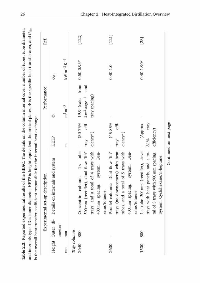
26 Chapter 2. Heat-Integrated Distillation Overview
Tabl
e2.
3.R
epor
ted
expe
rim
enta
lres
ults
ofth
eH
IDiC
.The
deta
ilson
the
colu
mn
inte
rnal
cove
rnu
mbe
rof
tube
s,tu
bedi
amet
er,
and
inte
rnal
sty
pe.
IDis
inne
rdi
amet
er,H
ETP
ishe
ight
-equ
ival
entt
heor
etic
alpl
ates
,Φis
the
spec
ific
heat
tran
sfer
area
,and
Uih
x
isth
eov
eral
lhea
ttr
ansf
erco
effic
ient
resp
onsi
ble
for
the
inte
rnal
heat
exch
ange
.
Expe
rim
enta
lset
-up
desc
ript
ion
Perf
orm
ance
Ref
.
Hei
ght
Out
erdi
-
amet
er
Det
ails
onin
tern
als
and
syst
emH
ETP
ΦU
ihx
mm
mm
mm
2m−
3kW
m−
2K−
1
Tray
colu
mns
2640
800
Con
cent
ric
colu
mn:
1×tu
be
500
mm
(rec
tifie
r),
dual
flow
"lif
t"
tray
s,an
da
tota
lof
4tr
ays
wit
h
400
mm
spac
ing.
syst
em:
Ben
-
zene
/tol
uene
.
-(5
0-75
%
tray
effi-
cien
cy*)
19.9
(cal
c.fr
om
4m
2st
age−
1an
d
tray
spac
ing)
0.50
-0.9
5*[1
22]
2600
-Pa
ralle
lco
lum
ns:
Dua
lflo
w"l
ift"
tray
s(n
odo
wnc
omer
s)w
ith
heat
tube
s,an
da
tota
lof
5tr
ays
wit
h
400
mm
spac
ing.
syst
em:
Ben
-
zene
/tol
uene
.
-(4
5-85
%
tray
effi-
cien
cy*)
-0.
40-1
.0[1
21]
1500
800
1×tu
be30
0m
m(r
ecti
fier)
,si
eve
tray
sw
ith
heat
pane
ls,
and
ato
-
talo
f3
tray
sw
ith
500
mm
spac
ing.
Syst
em:
Cyc
lohe
xane
/n-h
epta
ne.
-(A
ppro
x.
81%
tray
effic
ienc
y)
-0.
40-1
.90*
[28]
Con
tinu
edon
next
page

2.3. The Heat-Integrated Distillation Column 27
Tabl
e2.
3–
cont
inue
dfr
ompr
evio
uspa
ge
Expe
rim
enta
lset
-up
desc
ript
ion
Perf
orm
ance
Ref
.
Hei
ght
Out
erdi
-
amet
er
Det
ails
onin
tern
als
and
syst
emH
ETP
ΦU
ihx
mm
mm
mm
2m−
3kW
m−
2K−
1
Pack
edco
lum
ns19
00-
Shel
l-an
d-tu
be:
21×
300
mm
tube
s.
Syst
em:
Ben
zene
/tol
uene
.
0.42
0(t
ube)
and
0.33
0
(she
ll)
-0.
60-1
.0*
[118
]
16,0
0025
4C
once
ntri
c:1×
tube
wit
hva
ry-
ing
diam
eter
:14
0,16
5,an
d
190
mm
(rec
tifie
r)co
ntai
ning
MC
PAC
Kst
ruct
ured
pack
ing
(wid
est
inbo
ttom
).Sy
stem
:B
enze
ne/-
tolu
ene.
--
-[1
09,
66]
20,0
0031
8.5
Shel
l-an
d-tu
be:
3×10
1.6
mm
tube
s
(rec
tifie
r).
Syst
em:
Ben
zene
/-
tolu
ene.
0.29
*-
0.45
0-0.
600*
[123
]
20,0
0031
8.5
Con
cent
ric:
1×tu
be13
9.8
mm
(rec
tifie
r).
Syst
em:
Ben
zene
/-
tolu
ene.
0.26
*-
0.50
0-0.
810*
[123
]
Con
tinu
edon
next
page

28 Chapter 2. Heat-Integrated Distillation Overview
Tabl
e2.
3–
cont
inue
dfr
ompr
evio
uspa
ge
Expe
rim
enta
lset
-up
desc
ript
ion
Perf
orm
ance
Ref
.
Hei
ght
Out
erdi
-
amet
er
Det
ails
onin
tern
als
and
syst
emH
ETP
ΦU
ihx
mm
mm
mm
2m−
3kW
m−
2K−
1
20,0
0031
8.5
Con
cent
ric:
1×tu
be19
8m
m(r
ec-
tifie
r).
Syst
em:
Ben
zene
/tol
uene
.
0.27
*-
0.53
0-0.
810*
[123
]
27,0
001,
400
Shel
l-an
d-tu
be:
7×do
uble
-tub
e
(rec
tifie
r)pa
cked
colu
mn
in2x
35
theo
reti
cal
stag
es.
Syst
em:
C4-
C6
hydr
ocar
bon
mix
ture
.
0.77
(cal
c.
from
colu
mn
heig
ht)
1.9
(cal
c.
from
colu
mn
heig
htan
d
2.25
m2
stag
e−1 )
0.67
[58]
1,00
020
0
(wid
th)
Stru
ctur
edpl
ate-
fin:
40pa
r-
alle
lch
anne
ls(p
hase
con-
tact
528
m2
m−
3 ).
Syst
em:
Cyc
lohe
xane
/n-h
epta
ne.
1.20
-1.4
452
.70.
214-
0.32
1[1
9]
1,00
020
0
(wid
th)
Stru
ctur
edpl
ate-
pack
ing:
Cor
ru-
gati
ons
incl
ined
inop
posi
tes
dire
c-
tion
(pha
seco
ntac
t60
0m
2m−
3 ).
Syst
em:
Cyc
lohe
xane
/n-h
epta
ne.
0.22
-0.4
052
.70.
373-
0.55
0[1
9]
Con
tinu
edon
next
page

2.3. The Heat-Integrated Distillation Column 29
Tabl
e2.
3–
cont
inue
dfr
ompr
evio
uspa
ge
Expe
rim
enta
lset
-up
desc
ript
ion
Perf
orm
ance
Ref
.
Hei
ght
Out
erdi
-
amet
er
Det
ails
onin
tern
als
and
syst
emH
ETP
ΦU
ihx
mm
mm
mm
2m−
3kW
m−
2K−
1
1,00
015
0C
once
ntri
c:1×
inne
rtu
bew
ith
vary
ing
diam
eter
88-1
08m
m(I
D,
wid
esti
nbo
ttom
)w
ith
Dix
onpa
ck-
ing
and
150
mm
0.12
-0.1
5
(inn
er)
and
0.35
-0.5
9
(out
er)*
-0.
780-
1.00
(Eq
(2.5
))
[170
]
Com
bine
dtr
ayan
dpa
cked
colu
mns
6,80
025
0m
m(I
D)
Con
cent
ric:
Stri
pper
=O
uter
shel
l
wit
hpa
ckin
g(2
50m
m(I
D),
5.2
mhe
ight
).R
ecti
fier=
25tr
ays
inin
-
ner
tube
(150
mm
ID,6
.8m
heig
ht).
Syst
em:
Etha
nol/
wat
er.
-9.
6(c
alc.
from
0.09
426
m2
stag
e−1 )
0.32
49[8
1]
*Obt
aine
dfr
omfig
ure
inre
fere
nce

30 Chapter 2. Heat-Integrated Distillation Overview
2.3.2 Dynamic Modelling
In dynamic distillation column simulations, the "constant molar overflow" assump-
tion is widely applied. As a consequence, the energy holdup derivatives are con-
verted into algebraic equations [146]. This assumption has been adopted in a HIDiC
model by Huang et al. [60] and Liu et al. [92], which has been applied for both
static and dynamic applications. The models of Huang et al. and Liu et al. require
constant pressures in the two column sections and ideal mixtures, but these models
have proven useful in dynamic simulations and optimisation due to the low com-
putational efforts required. However, the models of Huang et al. [60] and Liu et
al. [92] do not take liquid and vapour hydraulics into account. In conventional
distillation columns, vapour dynamics are usually fast and have a minor impact on
the overall distillation column performance. However, the liquid hydraulics are im-
portant, as propagations of changes in the top of a real distillation column do not
affect the bottom immediately [147]. Because internal heat transfer causes local
pressure changes, it can be argued that both liquid and vapour hydraulics should
be accounted for in the dynamic modelling of the HIDiC. The expression for lin-
earised tray liquid hydraulics [151] was adopted by Zheng et al. [172] for a HIDiC,
while the Franscis weir formula is more common (used by e.g. Ho et al. [55]). Ho
et al. [55] included pressure hydraulics in their HIDiC simulation study by mod-
elling the propagation of pressures through each stage in the rectifying section as
having first-order dynamics. However, the impact of the propagation of pressure
changes in the stripping section was neglected in the study of Ho et al. [55]. The
concept of first-order dynamics in the pressure dynamics is similar to that of the
linearised tray liquid dynamics, but the pressure dynamics are occuring in a smaller
time scale. For conventional distillation columns, the first-order dynamic approx-
imation is typically adequate for describing the vapour dynamic responses [151].
Alternatively, the propagation of pressure in a HIDiC can be accounted for by cor-
relating vapour flow rates through pressure gradients between column stages as
Wang et al. [166]. For conventional distillation columns, a detailed dynamic model
is presented by e.g. Gani, Cameron and Ruiz [42, 21, 133], and Gross et al. [46].
2.3.3 Conceptual Design
The transition from conventional to the heat-integrated distillation configurations
result in a significantly higher number of design degrees of freedom. This leads to
complicated design problems. The methods for their solution often require models
for simulation. However, for binary mixtures, graphical design methods have been
described. In order for heat-integrated distillation configurations to become in-

2.3. The Heat-Integrated Distillation Column 31
creasingly recognised as a feasible alternative to conventional configurations, find-
ing a compromise between investment cost, operating cost and operability is essen-
tial.
Simulations of conventional distillation columns require specification of five
variables:
• Operating pressure
• Total number of stages
• Feed location
• Reflux ratio
• Vapour boil-up ratio
A common way of selecting these variables is using the McCabe-Thiele or Ponchon-
Savarit methods [54] for (pseudo)binary mixtures. The Fenske-Underwood-Gilliland
method applies to both binary and multicomponent mixtures but is limited to ideal
behaviours. These methods require specifications of the feed, the operating pres-
sure, and typically two product purities.
Assuming internal heat integration takes place between pairs of stages, the
HIDiC has additional degrees of freedom: The pressure ratio between the sec-
tions, the heat exchange area per pair, and the variables characterising the arrange-
ment of heat integration between the stages. In equilibrium stage-based distillation
column models, the assignment of heat-integrated stages contribute as additional
discrete variables to the existing discrete design variables, namely the number of
stages and the feed stage location. A complex combinatorial problem is resulted,
which has many alternative designs. It has been demonstrated that the pairing of
heat-integrated stages is crucial in obtaining an economically feasible HIDiC design
[158, 154]. This comprises a significant challenge to the HIDiC design because it is
not always recommended to pair all possible stages [23, 142, 51].
Approaches that do not rely on mathematical optimisation, commonly assume
uniform heat exchange areas or uniform heat duties throughout the heat-integrated
stages. However, optimal arrangements often involve non-uniform heat exchange
areas as well as non-uniform internal heat duties [155]. The optimum pressure
ratio differs little from the one required to obtain a minimum temperature driving
force between the paired stages [155].
Graphical design approaches for the HIDiC has been the focus of several works.
Takamatsu et al. [156] developed a stepping procedure resembling McCabe-Thiele
32 Chapter 2. Heat-Integrated Distillation Overview
constructions. Nakanishi et al. [118] proposed a relation between the minimum re-
flux ratio and the total heat exchange area for evaluation of the separation feasibil-
ity. Ho et al. [56] extended the Ponchon-Savarit graphical method to demonstrate
binary HIDiC design by the use of enthalpy-composition-diagrams (hxy-diagram).
By specifying the column section pressures and the amount of internal heat trans-
fer, constructions can be established in a fashion resembling that of a conventional
column design, leading to the required number of stages and feed stage location.
From these, the compressor duty and reboiler duty can be estimated, and the re-
quired heat exchange area can be calculated. Due to the simplicity of this method, a
constant heat duty on every pair (decision variable) is assumed and no suggestions
for the pairing of the stages for internal heat integration are provided. Later, the
Ponchon-Savarit method was slightly adjusted and a graphical tool was introduced
[159], called reversible distillation curves (RDCs). The RDCs were incorporated in
the hxy-diagram to guide the identification of thermodynamically preferred heat-
integrated stages. The extended Ponchon-Savarit method requires specifications of
the total number of stages, reboiler duty, the compressor duty, and the number of
heat-integrated stages, inspired by a corresponding design of a conventional col-
umn.
The discrete nature of the design problem has been tackled by reducing the
mixed integer non-linear mathematical programming (MINLP) problem into a con-
tinuous formulation by Harwardt and Marquardt [51]. The solution strategy for
this NLP is based on a superstructure optimisation approach to determine the op-
timal number of stages and the position and the heat transfer areas of internal
heat exchangers for both column sections. Solutions with the total annualised cost
(TAC) and the total energy consumption as objective functions were presented. The
advantage of using a mathematical formulation of the problem is the flexibility of
being able to impose e.g. physical constraints on the optimisation variables. The
MINLP was solved by Shahandeh et al. [140] by using a genetic algorithm and
innovative decision variables called "the layout numbers". Furthermore, a method
with an integrated Boltzmann Estimation of Distribution Algorithm was adopted
by Gutierrez-Guerra et al. [47] in order to solve the design problem as an optimi-
sation problem. Provided the simulation tools are accessible, these mathematical
programming-based methods can give relatively fast optimal CDiC, HIDiC, SRVC or
MVRC design solutions. However, due to the high degree of non-linearity imposed
by e.g. thermodynamic relations, the extensive number of discrete variables, and
the overall magnitude of the design problem of HIDiC configurations, advanced
and robust solution procedures are required. Optimal solutions in simulation stud-
ies agree that the internal heat exchange areas should be focused in the top of the

2.3. The Heat-Integrated Distillation Column 33
rectifying section (near conventional cold utility) and in the bottom of the stripping
section (near conventional hot utility) [51, 140, 47].
After specifying the heat-integrated stages, it has been proposed by Chen et al.
[23] and Gadalla [41] to reduce the number of heat-integrated stages taking the
ideal HIDiC as a reference. The design of the ideal HIDiC is in both cases based on
iterative algorithms requiring experience-based decisions on e.g. compression ratio
and pairing. Chen et al. [23] proposed an iterative algorithm requiring the designer
to specify the desired number of heat-integrated pairs (three by default) and then
modifying their locations by sensitivity analysis of a specified objective function.
Gadalla [41], on the other hand, propose to eliminate the pairs having the lowest
temperature driving forces, i.e. the pinched stages considering the impact on a
specified objective function. In addition, the method of Gadalla includes a hydraulic
feasibility analysis step, which provides a means of quantifying the feasibility of
different internal heat exchanger/column shell arrangements based on geometrical
considerations.
For the simpler configuration with only external heat integration between the
condenser and the reboiler as e.g. in the MVRC, a design procedure is proposed
by e.g. Omideyi et al. [127]. The SRVC is a combination of internal heat inte-
gration from the HIDiC and external heat integration from the MVRC. Hence, the
SRVC has two compressors and two throttling valves as indicated in Figure 2.4(b).
Simulations indicated that larger energy and cost savings can be obtained for some
separations in the SRVC compared to the HIDiC [31] and this type of heat inte-
gration was superior to a HIDiC with heat integration between reboiler and the
condenser realised only by increased compression ratio [98].
As shown, the topic of design of heat-integrated distillation columns, particu-
lar HIDiC, has been addressed by various methods. The methods can be resolved
into three classes, as reported in Table 2.4 together with literature examples and
pros and cons. Due to the significantly increased degrees of freedom, most meth-
ods have design decisions that require insights in the performance of the considered
configuration. In the graphical design methods, most design decisions are extensive
variables (duties or flows), which might lead to infeasible designs. For example, the
compressor duty in the extended Ponchon-Savarit method must be specified prior to
knowing the actual feasible temperature gradients for internal heat transfer. In the
simulation-based approaches, column profiles are available at each iteration step,
and thus decisions can be taken as the design gradually arises. Also the mathemati-
cal programming methods can cope with this. However, the solution algorithms are
tailored to the considered systems and the associated assumptions/simplifications.

34 Chapter 2. Heat-Integrated Distillation Overview
Table 2.4. Design methods overview with their pros and cons.
Class Method and, ref-erence
Pros Cons
Graphical • McCabe-Thiele[156]
• Ponchon-Savarit [56]
• ExtendedPonchon-Savarit [159]
• Intuitive• Balance equa-
tions aresolved graphi-cally
• Limited to(pseudo)binarymixtures (2D repre-sentations)
• Risk of infeasible de-sign
• Decision variablesdirectly related toenergy or massbalances (flows orduties)
MathematicalProgram-ming
• Superstructureoptimisation[51]
• Genetic Algo-rithm [140]
• BUMDA Algo-rithm [47]
• Generic andflexible costfunction andconstraints
•Multicomponentmixtures
• Requires full modelimplementation
• Convergence of non-linear problem
• Appearance of flatand/or local minima
Simulation-based
• SimplifiedHIDiC [23]
• Thermo-hydraulicApproach [41]
• Incrementaldesign
•Multicomponentmixtures
• Requires full modelimplementation
• Convergence (with-out optimiser)
2.3.4 Equipment Design
The distillation equipment, which is affected by the introduction of internal heat
integration in the HIDiC is discussed in this section. This covers the column in-
ternals and the possibilities for realising internal heat transfer inside the internals.
Moreover, new equipment is introduced compared to conventional distillation. A
compressor is required to realise internal heat transfer and a throttling valve is re-
quired to reduce the pressure of the liquid entering the low-pressure section from
the high-pressure section. Details about the choice of e.g. compressor is rarely
mentioned in the HIDiC literature. However, it has a consequence for the economic
models. Therefore this subsection provide suggestions for suitable equipment for
the HIDiC application.

2.3. The Heat-Integrated Distillation Column 35
2.3.4.1 Compressor
Two different groups of commercially available compressors are existing: Rotody-
namic compressors and positive displacement compressors. The rotodynamic com-
pressors have rotating parts, which translates motion into momentum in the gas
particles and ultimately into pressure. As a result, the gas flow is continuous. The
positive displacement compressors work, as the name implies, by directly increas-
ing pressure by displacing gas volumes. Such compressors operate at fixed gas flow
rate but high pressure differentials can be achieved. The two groups of compressors
can further be divided into the following types [162]:
• Rotodynamic types:
– Centrifugal compressor, producing radial discharge flow at a high flow
rate and a compression ratio of up to 4.5.
– Axial flow compressor, which can handle large flow rates and small com-
pression ratios in the range of 1.2-1.5 (or up to 5-6.5 per machine con-
sisting of several stages). Axial flow compressors have higher efficiencies
than centrifugal compressors but their stable operation ranges are rela-
tively narrow.
• Positive displacement types:
– Reciprocating piston compressors operate at low gas flow rates and rela-
tive large compression ratios (up to 10).
– Rotary compressors (screws, blades, lobes etc.), can boost the discharge
pressures by up to 690 kPa thereby providing very large compression ra-
tios for smaller throughput. Such compressors are typically used for
vacuum services operating at high efficiencies around 80-95%.
The centrifugal/motor type compressor appears to be most suited type in distilla-
tion processes due to the high vapour capacity and the robustness under varying
flow rates. A compression ratio limit of up to five should be sufficient for the HIDiC.
Compression ratios above five are expected to become economically infeasible due
to both high operation cost and high investment cost. Sulzer [49] reports that
the compressor types turboblowers, radial turbo compressors, screw-type or axial
compressors are used for heat pump-assisted distillation (e.g. MVRC and VCC ap-
plications). These are mainly rotodynamic type compressors.
The relevant models for the HIDiC application is the temperature change for a
giving compression ratio and the required compressor duty. These can be modelled

36 Chapter 2. Heat-Integrated Distillation Overview
by considering an ideal gas and by introducing an isentropic efficiency [162]. From
thermodynamic analysis, the discharge temperature and the compression duty are:
Tout = Tin
(1+
1ηis
[(Pout
Pin
)(k−1)/k
−1
])(2.1)
E =1
ηis
(k
k−1
)RTin
[(Pout
Pin
)(k−1)/k
−1
](2.2)
k =CV
P
CVV=
CVP
R−CVP
(2.3)
where
Tout = outlet (discharge) temperature [K]
Tin = inlet temperature [K]
E = work of compression [kW]
ηis = isentropic effeciency (isentropic work divided by actual work) [-]
Pout = outlet (discharge) pressure [kPa]
Pin = inlet pressure [kPa]
CVP = constant pressure heat capacity [kJmol−1 K−1]
CVV = constant volume heat capacity [kJmol−1 K−1]
R = universal gas constant [kJmol−1 K−1]
Equations (2.1)-(2.2) are based on isentropic efficiencies and these equations typ-
ically appear in the HIDiC literature [112, 51]. However, the efficiency of a com-
pressor is an empirically derived quantity and thus depends on the compressor lay-
out/type. It is therefore believed that the precision loss related to the selection of a
constant efficiency makes it unnecessary to account for vapour phase non-ideality.
In modelling, Eq. (2.2) is therefore found sufficient.
When it comes to operation of a compressor, Muhrer et al. [107] considered
different operation modes of the compressor in an MVRC. They showed that a com-
pressor variables speed mode and a mode, where the integrated heat exchange area
was adjusted, were the best operation mode alternatives of the MVRC to compen-
sate for disturbances. Hence, in dynamic modelling of a compressor, it is important
to incorporate the compressor duty as a possible actuator variable, as it closely re-
sembles the variable speed mode. A detailed dynamic model of a compressor is
formulated by Jiang et al. [76]. They show that the compressor time constants are
in the order of fractions of a second. Therefore, it is expected that the dynamics
of a compressor, as an actuator, are unimportant in the dynamic simulations of e.g.
the HIDiC.

2.3. The Heat-Integrated Distillation Column 37
2.3.4.2 Internal Heat Exchangers
Introducing heat transfer inside equipment, which conventionally is designed to
provide mass transfer (separation) using phase contact, involves a risk of arriving
at a trade-off between mass transfer and heat transfer efficiencies. In conventional
heat exchangers, compact plate-and-fin heat exchangers can achieve specific heat
exchange areas up to 1200 m2 m−3 while shell-and-tube heat exchangers can achieve
up to 300 m2 m−3 [162]. When heat transfer is combined with mass transfer, approx-
imate specific heat exchange areas from 1.9 m2 m−3[58] and up to 52.7 m2 m−3[19]
have been reported (Table 2.3). Higher numbers are in practice difficult to achieve
in distillation, since the liquid flow pattern is difficult to alter because gravity is the
only driving force for the liquid flow. In conventional heat exchangers, baffles are
being used in the shell side in order to effectively increase the possible contact area
with the tube side. Note that the specific area is reported in heat exchange area
per column volume. Alternatively this number could be reported per column area.
However, in order to compare structured columns with tray columns, the third di-
mension (height) is important due to physical limitations in the different internals
layout.
Table 2.5 reports the encountered arrangement suggestions for realising internal
heat integration in distillation. The arrangements can be classified in dividing wall
arrangement, which is suited for both tray columns and packed columns, and the
partitioning wall arrangement, which can only be employed with packed columns.
However, as the Table 2.5 clearly shows, most attention has been paid to the concen-
tric column and the shell-and-tube arrangements, both inspired by the conventional
shell-and-tube heat exchangers. As heat exchange takes place in the height of the
column, gradual condensation and vaporisation occurs inside the column. Hence,
the ideal diameter varies along the column height. For the concentric arrangement,
this corresponds e.g. to an inner rectifying section with a diameter, which is small
in the top and increases towards the bottom. In practice, the construction of such
tubes is particularly challenging [109], but this challenge has been overcome more
recently [170]. A simpler arrangement, yet effective, is the structured plate column
arrangement proposed by Bruinsma et al. [19]. This arrangement has the highest
reported specific heat transfer area among the experimental columns.
If the tube walls do not provide sufficient heat transfer area, heat panels can be
installed inside the trays [27, 28]. Gadalla et al. [37] used geometrical considera-
tions to propose relations of maximum achievable internal heat transfer area when
including heat panels for a concentric arrangement based on the column dimen-
sions. These relations are described in detail in Section 3.4.3, as they are used to
evaluate the feasibility of conceptual HIDiC designs.

38 Chapter 2. Heat-Integrated Distillation Overview
The challenge in achieving a sufficient heat exchanger area can be overcome in
the separate columns type (Table 2.5). One way of realising this arrangement is
to withdraw liquid from the holdup of one tray in the high-pressure column and
let it exchange heat with the holdup of a tray in the low-pressure column. This
can be done using a conventional heat exchanger located outside both columns or
inside in either of the columns. The latter option has been patented by Wakabayashi
and Nakao [161], in which stabbed-in type heat exchangers were inserted in the
trays of the high-pressure section. However, the application of stabbed-in type heat
exchangers is limited to cases, where only a few trays are heat integrated. De Koijer
et al. [25] presented an alternative to the stabbed-in type heat exchanger, which is
suitable for sieve trays. This alternative consisted of coils, hanging slightly above
the tray, containing a cooling media. This configurations corresponds to the DSHE
but the principle can also be transferred to the HIDiC configuration.
A trend in the layout of the experimental HIDiC studies is the small employed
diameter-to-height ratios (heights and diameters are reported individually in Ta-
ble 2.3). Consider for example the tallest reported packed HIDiC with a height
of 27.000 mm and a diameter of 1.400 mm resulting in a diameter-to-height ratio
of 0.05. None of the reported experimental experiences concern industrial-scale
equipment, in which only the dividing wall constitutes the heat exchange area (Ta-
ble 2.3). This comprises an issue when evaluating the technical feasibility of the
HIDiC, as the achievable heat transfer area, in many cases, decreases with increas-
ing column diameter. The specific heat exchange area for example a shell-and-tube
arrangement is given by:
Φ =NtubesπdiH
πd2oH/4
=4Ntubesdi
d2o
(2.4)
where
Φ = specific heat transfer area (heat exchange area per column volume)
[m2 m−3]
Ntubes = number of tubers inside the column shell [-]
di = inner (tube) diameter [m]
do = outer (shell) diameter [m]
H = height of control volume [m]
In a conventional distillation column, the required tray cross sectional area typically
scales linearly with the internal vapour flow rate, which scales linearly with the feed
flow rate (throughput). In order to maintain the same internal heat transfer rate
during scale-up, provided that the temperature driving force remain constant, the
specific heat exchange area must remain constant. This means that the heat ex-
change area must be proportional to the feed flow rate. In the simple case of a

2.3. The Heat-Integrated Distillation Column 39
concentric arrangement (Ntubes = 1), the specific heat exchange area in Eq. (2.4)
does not satisfy this requirement as argued in Illustration 2.1. By designing a dis-
tillation column with small diameter, the specific heat exchange area can be large.
But in the bulk chemical industry, the conventional column areas can exceed 14 min diameter and 100 m in elevation [153]. As heat panels inside a distillation col-
umn has proven efficient [28] for tray columns, such installations has not been
encountered for packed columns.
A correlation between the overall heat transfer coefficient (Uihx) and the com-
pression ratio (CR) has proposed by Xu et al. [170]:
Uihx = 4.139−4.154CR+1.290CR2 kWK−1 (2.5)
CR = compression ratio [-]
Despite the fact that it is based on an ethanol/water mixture in a concentric packed
column, the tendency of decreasing overall heat transfer coefficient with increasing
compression ratio (or increasing temperature driving force) has been confirmed for
tray columns elsewhere [27]. The appearing of dry spots on the heat exchange sur-
face was believed to cause this decreasing trend, which might represent a significant
challenge in industrial set-ups.
2.3.4.3 Column Internals
In conventional distillation columns, the phase contact between the liquid and the
vapour is crucial for the separation performance. Different means of creating phase
contact are:
• Tray/plate columns (sieve, valve or bubble-cap): The column is vertically di-
vided in sub volumes called the trays, which makes accessibility and, thus,
maintainance easy. The most common types are: Sieve trays, valve and
bubble-cap trays. Some typical dimensions are [162]: Weir heights are 50.8 mm,
weir lengths about 75% of tray diameter. Pressure drop per tray is of the or-
der of 0.70 kPa. Sieve tray perforations are 6.35-12.7 mm diameter with hole
area being 10% of the active cross section. Single-pass sieve and valve trays
with crossflow are the most widely used trays [57].
• Packing (random or structured): These type of columns often has a high spe-
cific area for separation (contact area per column volume). They have low
pressure drops and low holdups, and they are typically used for low column
diameters, low pressures, or when proof materials are required. However,
liquid maldistribution can be a limitation and the prices are typically higher
than tray columns [162].

40 Chapter 2. Heat-Integrated Distillation Overview
Table 2.5. Suggestions for realisation of internal heat exchangers. The table col-umn "origin" refers to the literature, in which the arrangement was proposed.
Class Cross section Type References
Origin Experimental
Dividingwall
Separate columns [52,117,161]
[25, 121]
Partitioning wallcolumn
[138,75]
Concentric col-umn
[45,24]
[28, 66,81, 170,81, 122][132]*
Partitioningwall
Multiconcentriccolumn
[124]
Shell-and-tubecolumn
[7] [109, 123,66, 58]
Structured platecolumn
[4] [19]
Singletower
Alternating trays [71]
* Simulated experiments using computational fluid dynamics
The question remains, how does the introduction of internal heat exchangers affect
the separation and what is possible in conventional equipment? The answers de-
pend on many factors such as how much heat transfer area is required and what
is the column cross sectional area etc. It has been found that heat panels lead to
a slightly increased tray separation efficiency (10%), which could be due to the
hindrance of backmixing of the froth [28]. Furthermore, the pressure drops in the
concentric sieve trays are independent of the presence of heat panels [27].
For packed columns, a decrease in the separation efficiency in the outer column
(concentric arrangement) is observed [170]. This decrease is separation efficiency
is believed to be caused by liquid accumulation (maldistribution) near the inner col-
2.3. The Heat-Integrated Distillation Column 41
umn wall due to its increasing diameter towards the bottom. In the structured plate
arrangement, also no significant impact on the separation efficiency was observed
for neither stripping nor rectifying operations [19].
2.3.5 Benchmark Studies
Various studies concern benchmarking of the HIDiC but the overall conclusion are
often contradictory due to numerical dissimilarities (in e.g. overall heat transfer co-
efficients and utility prices) and different basis of comparisons.This was for example
discussed in relation to the achievable heat exchange area in section 2.3.4.2.
The steady state performances of simulation and experimental studies of the
HIDiC compared to the CDiC are summarised in Table 2.6 based on a variety of
literature sources. Since the internal heat transfer is a key element in such studies,
the parameters related to this, namely the internal heat exchange area(s) and the
overall heat transfer coefficient(s), are reported along with the simulation results
(if stated).

42 Chapter 2. Heat-Integrated Distillation Overview
Illustration 2.1. Dependence of specific area on column diameter in the con-
centric arrangements.
Consider a larger and a smaller concentric HIDiC with trays of the dimensions
given in the below:
Di Do di doAi ai
Ao ao
Assume that the required active area of a tray is proportional to the vapour flow,
that the molar vapour flows are identical in each of the sections (inner and outer
tube) and that the temperatures are similar (applies to close-boiling component
separations). If the HIDiC is operated at a compression ratio of two, which is a
common value, then the density of the vapour in the inner tube is twice of that
in the outer tube when considering ideal vapour phases. The ratio between the
temperatures in the inner section and the outer section is approximately unity
since small temperature driving forces are preferred for internal heat integra-
tion. Therefore the volumetric vapour flow in the outer tube is twice that of in
the inner tube, and similarly the tray area of the outer tube is twice of that of
the inner tube. This translates into
Ao = 2Ai, ao = 2ai⇒Do =
√2Di, do =
√2di,
which, when combining with Eq. (2.4), gives
Φ|Do=5m = 2/Do = 0.4m2 m−3
Φ|do=0.5m = 2/do = 4m2 m−3
Hence, the smaller column has a larger available, specific heat exchange area.
Provided the given assumptions apply, the ratio of the specific heat transfer areas
scales linearly with the ratios of the outer column diameters.

2.3. The Heat-Integrated Distillation Column 43
Tabl
e2.
6.B
ench
mar
king
ofth
eH
IDiC
.Sy
mbo
ls:
Aih
xis
the
heat
exch
ange
area
per
stag
e,U
ihx
isth
eov
eral
lhe
attr
ansf
er
coef
ficie
nt.
Inso
me
case
s,on
lyth
epr
oduc
tU
ihxA
issu
pplie
d.Th
een
ergy
and
econ
omic
savi
ngs
are
repo
rted
wit
hre
fere
nce
to
aC
DiC
perf
orm
ing
the
sam
ese
para
tion
;po
siti
vesa
ving
sar
ein
favo
urof
the
HID
iC.E
lect
rica
lene
rgy
isw
eigh
ted
bya
fact
orof
thre
efo
res
tim
atin
gth
eto
tale
nerg
yco
nsum
ptio
nin
the
HID
iC.
Syst
emPa
ram
eter
sSa
ving
sR
ef.
Des
ign
para
met
ers
Uih
x
[kW
m2
K−
1 ]
Ener
gyEc
onom
y
Bina
rym
ixtu
res
Ben
zene
/tol
uene
UA=
10.0−
23.0
kWK−
140
%-
[114
]
--
40%
-[1
09]
A=
20m
2>
0.80
035
%-
[118
]
*-
-40
%-
[66]
∑A=
229.
7m
2-
--4
5%[1
39]
Opt
imal
desi
gn-
--1
1%[5
1]
Ace
tic
acid
/ace
tic
anhy
drid
eA=
270−
1000
m2
/A=
50−
420
m2
0.6
4%-
[22]
Prop
ylen
e/pr
opan
eA=
399
m2
/A=
779
m2
1.0
-35
%[1
25]
A=
400
m2
1.0
25%
vs
MV
RC
20%
vs
MV
RC
[158
]
∑A=
46.2
77m
2-
-35
.6%
[139
]
A=
18.5
8m
20.
5678
13%
-[9
4]
Ben
zene
/flu
orob
enze
neO
ptim
alde
sign
--
44%
[51]
Con
tinu
edon
next
page

44 Chapter 2. Heat-Integrated Distillation Overview
Tabl
e2.
6–
cont
inue
dfr
ompr
evio
uspa
ge
Syst
emPa
ram
eter
sSa
ving
sR
ef.
Des
ign
para
met
ers
Uih
x
[kW
m2
K−
1 ]
Ener
gyEc
onom
y
Ben
zene
/ch
loro
benz
ene
Opt
imal
desi
gn-
--1
7%[5
1]
Ben
zene
/n-h
epta
neO
ptim
alde
sign
--
46%
[51]
Cyc
lohe
xane
/n-h
epta
ne*
A=
21m
2(g
iven
53m
2m−
3an
d
HET
P)
0.3-
0.5
65%
40%
[19]
Ethy
lene
/eth
ane
A=
18.5
8m
20.
5678
-22%
-[9
4]
Tran
s-2-
bute
ne/
cis-
2-bu
tene
A=
18.5
8m
20.
5678
6%[9
4]
Met
hano
l/w
ater
A=
5499
1.4
m2
(1in
tern
alH
EX)
0.8
56%
27.2
%[1
41]
Etha
nol/
wat
erO
ptim
alde
sign
-38
%6%
[51]
*0.
0942
60.
3249
--
[81]
Mul
tico
mpo
nent
mix
ture
sB
enze
ne/t
olue
ne/p
-xyl
ene
Uih
xA=
0.5
kWK−
1-
34%
-[6
7]
n-pe
ntan
e/cy
clop
enta
ne/
2-
met
hylp
enta
ne
UA=
0.9
kWK−
1-
51%
-[6
8]
Prop
ane/
n-bu
tane
/n-p
enta
neU
ihxA
=6.
33kW
K−
1-
39%
2%[8
4]
12hy
droc
arbo
ns*
--
52%
[67]
Styr
ene/
benz
ene/
tolu
ene/
ethy
l-
benz
ene
Opt
imal
desi
gn-
74%
37%
[51]

2.3. The Heat-Integrated Distillation Column 45
The utility prices comprise the basis of economic benchmarking. Utility prices
vary with time and location because they depend on various factors such as avail-
ability, feedstock source, tax regulations, inflation and more. In fact, large instal-
lations often negotiate electricity price levels. Especially steam, produced in excess
locally, will reduce the price significantly. The benchmark studies report different
utility prices, which is illustrated in Table 2.7. In estimations of the operating costs
of distillation column configurations with compressors, the ratio of electricity cost
to steam cost is of utmost importance as the electricity usually is several times more
expensive than steam. This ratio can bias a conclusion towards a particular con-
figuration. For example, a high ratio favours a CDiC, while a low ratio potentially
favours heat pump-assisted configurations (MVRC, HIDiC etc.). This ratio is pro-
vided in Table 2.7 along with utility prices and the references. It can be seen that
the ratio varies from 1.8 and up to 23.3. Furthermore, this ratio is also commonly
used to scale the relative contributions of the duties (reboiler duty and compressor
duty) when reporting energy savings (Table 2.6). Hence, a consistent treatment
of this ratio is essential in the benchmarking of distillation column configurations.
Even in benchmarking studies, electrical energy weight factors from one to three
are observed, which complicates direct comparisons of the reported energy savings.
In Table 2.6, all duties were identified and converted into unified energy saving
measures using a factor of three.
Ulrich and Vasudevan [157] provide correlations for estimating electricity, steam
and cooling water prices based on the following expressions:
Selectricity = 1.3 ·10−1(CR PCI)+0.010(Ss, f ) (2.6)
Ssteam = 2.7 ·10−5m−0.9steam(CR PCI)+(0.0034P0.05
steam)(Ss, f ), (2.7)
1 < Psteam < 46barg, 0.06 < msteam < 40kgs−1
Scw = (0.0001+3.0 ·10−5v−1cw )(CR PCI)+0.003(Ss, f ), (2.8)
0.01 < vcw < 10m3 s−1
Where
Selectricity = electricity price [$kWh−1]
CR PCI= historical inflation parameter for projects in the U.S. [-]
Ss, f = fuel price [$GJ−1]
Ssteam = steam price [$kg−1]
msteam = nominal steam production rate [kgs−1]
Psteam = steam pressure [barg]
Scw = cooling water price [$m−3]
vcw = nominal cooling water production rate [m3 s−1]
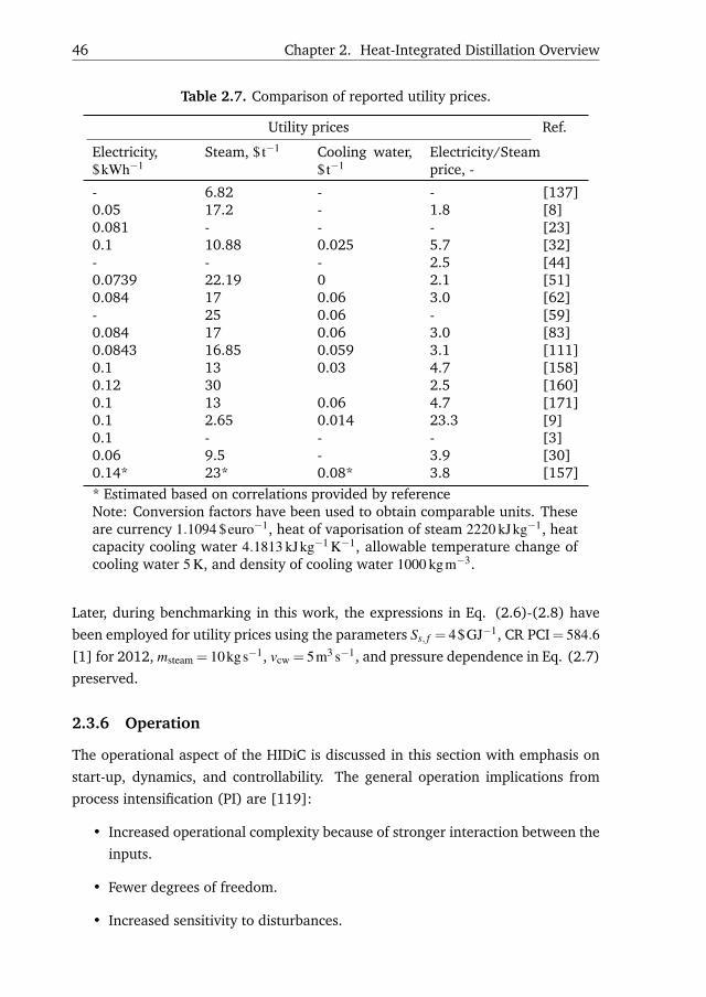
46 Chapter 2. Heat-Integrated Distillation Overview
Table 2.7. Comparison of reported utility prices.
Utility prices Ref.
Electricity,$kWh−1
Steam, $t−1 Cooling water,$t−1
Electricity/Steamprice, -
- 6.82 - - [137]0.05 17.2 - 1.8 [8]0.081 - - - [23]0.1 10.88 0.025 5.7 [32]- - - 2.5 [44]0.0739 22.19 0 2.1 [51]0.084 17 0.06 3.0 [62]- 25 0.06 - [59]0.084 17 0.06 3.0 [83]0.0843 16.85 0.059 3.1 [111]0.1 13 0.03 4.7 [158]0.12 30 2.5 [160]0.1 13 0.06 4.7 [171]0.1 2.65 0.014 23.3 [9]0.1 - - - [3]0.06 9.5 - 3.9 [30]0.14* 23* 0.08* 3.8 [157]* Estimated based on correlations provided by referenceNote: Conversion factors have been used to obtain comparable units. Theseare currency 1.1094 $euro−1, heat of vaporisation of steam 2220 kJkg−1, heatcapacity cooling water 4.1813 kJkg−1 K−1, allowable temperature change ofcooling water 5 K, and density of cooling water 1000 kgm−3.
Later, during benchmarking in this work, the expressions in Eq. (2.6)-(2.8) have
been employed for utility prices using the parameters Ss, f = 4$GJ−1, CR PCI= 584.6[1] for 2012, msteam = 10kgs−1, vcw = 5m3 s−1, and pressure dependence in Eq. (2.7)
preserved.
2.3.6 Operation
The operational aspect of the HIDiC is discussed in this section with emphasis on
start-up, dynamics, and controllability. The general operation implications from
process intensification (PI) are [119]:
• Increased operational complexity because of stronger interaction between the
inputs.
• Fewer degrees of freedom.
• Increased sensitivity to disturbances.
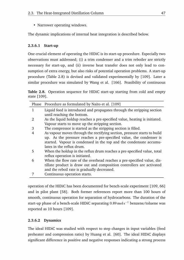
2.3. The Heat-Integrated Distillation Column 47
• Narrower operating windows.
The dynamic implications of internal heat integration is described below.
2.3.6.1 Start-up
One crucial element of operating the HIDiC is its start-up procedure. Especially two
observations must addressed; (i) a trim condenser and a trim reboiler are strictly
necessary for start-up, and (ii) inverse heat transfer does not only lead to con-
sumption of extra energy, but also risks of potential operation problems. A start-up
procedure (Table 2.8) is devised and validated experimentally by [109]. Later a
similar procedure was simulated by Wang et al. [166]. Feasibility of continuous
Table 2.8. Operation sequence for HIDiC start-up starting from cold and emptystate [109].
Phase Procedure as formulated by Naito et al. [109]
1 Liquid feed is introduced and propagates through the stripping sectionuntil reaching the bottom.
2 As the liquid holdup reaches a pre-specified value, heating is initiated.Vapour starts to move up the stripping section.
3 The compressor is started as the stripping section is filled.4 As vapour moves through the rectifying section, pressure starts to build
up. As the pressure reaches a pre-specified value, the condenser isstarted. Vapour is condensed in the top and the condensate accumu-lates in the reflux drum.
5 When the holdup in the reflux drum reaches a pre-specified value, totalreflux operation is initiated.
6 When the flow rate of the overhead reaches a pre-specified value, dis-tillate product is draw out and composition controllers are activatedand the reboil rate is gradually decreased.
7 Continuous operation starts.
operation of the HIDiC has been documented for bench-scale experiment [109, 66]
and in pilot plant [58]. Both former references report more than 100 hours of
smooth, continuous operation for separation of hydrocarbons. The duration of the
start-up phase of a bench-scale HIDiC separating 0.89 mols−1 benzene/toluene was
reported as 10 hours [109].
2.3.6.2 Dynamics
The ideal HIDiC was studied with respect to step changes in input variables (feed
preheater and compression ratio) by Huang et al. [60]. The ideal HIDiC displays
significant difference in positive and negative responses indicating a strong process
48 Chapter 2. Heat-Integrated Distillation Overview
non-linearity. Furthermore, strong input-output interactions were found. The anal-
ysis was extended to cover dynamic responses of all feed flow rates, feed composi-
tion, feed thermal condition, section pressures, and heat exchange area per stage
resulting in the same conclusion, i.e. strong non-linearity is present [92]. How-
ever, it was noticed that the ideal HIDiC is a self-balancing process. The process
is self-balancing in the sense that effects of disturbances in the feed are reduced
compared to conventional distillation columns. This can be illustrated by the exam-
ple of increased feed flow rate. If the feed is composed of both liquid and vapour,
the concentration of the heavy component increases in the rectifying section and
decreases in the stripping section. This leads to increased internal heat transfer,
which has the opposite effect of the composition responses.
Simulations showed that high purity HIDiC has slower responses and stronger
non-linearity [173] leading to e.g. asymmetric and inverse composition responses.
The inverse responses were concluded to be severe for responses in the top com-
position subject to changes in the feed thermal condition and thus, using the feed
duty is manipulated variable is not recommended for feedback control [173]. A
similar significant increase in the process non-linearity is also observed for conven-
tional distillation [35]. Usually fast control action can reduce model mismatch by
keeping the process operated close to the nominal operating point, where the effect
of non-linearity is least.
Steady state multiplicity is well documented for the CDiC (e.g. Jacobsen and
Skogestad [69]). Doherty and Perkins [29] report that no steady state multiplicity
occurs for binary distillation in the case of constant molar overflow (CMO) assump-
tion or in a ternary flash unit but only occur in ternary distillation. Multiple steady
states are also reported for e.g. the VCC [90]. Furthermore, simulation results
suggest that steady state multiplicity also occurs for the HIDiC [79]. The pres-
ence of steady state multiplicity depends on the HIDiC control structure and the
operation policy and, in particular, strongly depends on the compressor operating
policy. Hence, it is recommended to operate the compressor at a fixed duty or rota-
tion speed rather than a fixed compression ratio [79, 96]. Alternatively, DV or LB
control structures for composition control can be adopted for avoiding steady state
multiplicity [165]. Later, Kano et al. [80] developed a graphical instability criteria
for the HIDiC.
2.3.6.3 Controllability
Nakaiwa et al. [110] considered the general HIDiC with four variables controlled,
namely the distillation composition, the bottoms composition, the reflux drum
holdup and the reboiler holdup using single input-single-output (SISO) controllers

2.4. Research Areas 49
paired with four of the candidates u = [D,B,Lcnd ,Vrbl ,Lcnd/D,Vrbl/B,∆P, fF ]. The
reboil flow rate (Vrbl) is used instead of the reboiler duty (Qrbl), the pressure el-
evation (∆P) is used instead of the compressor duty (E), and the feed thermal
condition ( fF) is used instead of feed preheater (QF). All stabilising control loops
were assumed perfectly controlled and no further attention was paid to these. The
present control problem has 70 possible solutions and it was solved by evaluating
steady state control performance indices including the condition number (CN) and
the relative gain array (RGA). The study showed that the feed preheater and the
compressor are feasible candidates as manipulated variables for dual composition
control. In addition, a conventional control scheme such as dual ratio control is
feasible in the HIDiC. Closed-loop simulation showed that control schemes utilising
fF or ∆P have oscillatory servo and regulatory responses. This is not surprising as
fF has a direct impact on the overall mass balance on the column affecting both
composition while ∆P also affects both compositions by only affecting the internal
flows. Especially, the control schemes including fF as a manipulated variable show
strong interactive behaviour, as changes in external flows have significantly larger
impact on compositions than internal flows [151]. It was shown that the operability
of the HIDiC was more complicated than that of a CDiC due to diabatisation, while
closed-loop simulations confirmed this analysis [36].
Various authors have investigated PI-controllers for composition control in the
HIDiC and demonstrated stable operation by simulation of simple models [92, 173,
116, 174]. Huang et al. [63] used temperature to infer compositions and concluded
that simple temperature control (STC) can not work as effectively as in conventional
distillation columns. A similar temperature control scheme was adopted by Ho et al.
[55] using a more rigorous model accounting for pressure dynamics with acceptable
control performance.
2.4 Research Areas
Based on the presented literature review, the following topical conclusions related
to the state-of-the-art research can be made:
• Equipment design: Centrifugal compressors are suitable for heat pump ap-
plications due to moderate compression ratios and high allowable throughput.
Based on the required heat exchange areas, it appears that relatively large in-
ternal heat transfer areas are required. Therefore, focus should be directed
towards experimental set-ups with more industrially relevant dimensions. In
particular, the specific heat transfer area is relatively small for the majority of
the experimental set-ups, which indicates that one tube in a concentric dis-

50 Chapter 2. Heat-Integrated Distillation Overview
tillation column does not provide sufficient heat transfer area. Adding heat
panels inside the column can significantly improve the specific heat transfer
area without affecting the separation, but it has only been investigated in tray
columns. In packed columns, the structured plate HIDiC can provide excep-
tional high specific heat exchange areas. This topic of equipment design not
covered further in this work.
• Modelling and parameters: It appears that there is a mismatch in the re-
ported dynamic simulation results. The literature related to dynamic mod-
elling spans from simple models ignoring pressure dynamics and employ the
"constant molal overflow" assumption, whereas other models address these
simplifications to some extent. This leads to different conclusions when it
comes to the controllability and the development of control structures for
the HIDiC. One physical parameter of particular significance is the overall
heat transfer coefficient. This has been found to depend on operation condi-
tions and column arrangement. Based on reported literature values in Section
2.3.1, a value of 0.60 kWm−2 K−1 appears to be a representative value.
• Conceptual design: Many alternative design approaches exist. The differ-
ent approaches are classified in graphical methods, simulation-based methods
and mathematical programming-based methods. Different classes are suited
for different applications depending on the modelling and simulation efforts.
However, a common denominator of the described methods is that they all re-
quire expert decisions due to the large number of design degrees of freedom.
• Controller design: Followed by the conceptual design, a design of instrumen-
tation and controllers is often followed. A formulation of the control structure
and philosophy must be conducted and evaluated for models accounting for
pressure dynamics, in particular. No literature has been encountered, which
addresses the root of this problem, i.e. how to obtain a stabilising control
structure in a systematic manner. After stable operation is ensured, addi-
tional control objectives can be investigated (purity control etc.). In addition,
the stabilising control structure is of utmost importance in industrial context
due to operational and safety concerns.
• The HIDiC among alternatives: It is clear that the HIDiC, in many appli-
cations, is an energy-wise and economically preferred alternative to conven-
tional distillation. However, many authors includes only the conventional
distillation column when benchmarking the HIDiC instead of including the
simpler MVRC, which is already used in the industry. It has also been found,

2.4. Research Areas 51
that comparing results across references is essentially impossible, since the
benchmark study conclusions are very case specific due to the significant vari-
ations in the economic parameters.
The present conclusions can be considered as a more detailed motivation for the
research targeted in this thesis. The order of the presented conclusions, closely
resembles the structure of the thesis in terms of the covered topics. However, the
first topic of experimental validation is not covered in this thesis, as relevant set-ups
have not been available.


Chapter3
Distillation ColumnModel
A generic model of the conventional, the heat-integrated, the
mechanical vapour recompression distillation columns, and re-
lated configurations, is presented. The solution procedure of
the model is outlined and illustrated using examples.
The model is different from the existing literature for four
reasons. The first reason relates to the way the compressor
model is incorporated in relation to the dynamic energy bal-
ances. Second, the way pressure dynamics are accounted for,
which is because of the former reason and the incorporation
of a well-known expression for vapour flow through perfora-
tions. Third, the high degree of detail in the description of the
trays, which enables investigation of entrainment flooding and
weeping. And finally, the fact that the model is formulated in
a generic framework, which is tailor-made for benchmarking of
heat-integrated distillation column configurations. Thus, while
many of the phenomena accounted for within the modelling
framework have appeared before in other contexts, they have
not been combined together in a consistent framework that puts
things on suitable form for maximum utility. The BP method of
Wang and Henke [163] for conventional distillation columns
is extended here such that it can cover the considered heat-
integrated distillation columns. An effective tear variable ini-
tialisation procedure was developed and provided along with
the method documentation. Experience using an extended ver-
sion of the BP method has been reported by Mah et al. [94].
54 Chapter 3. Distillation Column Model
However, it does not seem to have been documented in the open
literature.
The main contribution of this chapter is published in an article
[T. Bisgaard, J.K. Huusom, and J. Abildskov. Modeling and anal-
ysis of conventional and heat-integrated distillation columns.
AIChE Journal, 61(12):4251–4263, 2015]. An early state of the
model was published for the DYCOPS 2013 proceedings [T. Bis-
gaard, J.K. Huusom, and J. Abildskov. A modeling framework
for conventional and heat integrated distillation columns. 10thIFAC International Symposium on Dynamics and Control of Pro-cess Systems – Mumbai, India, pages 373–378, 2013].

3.1. Introduction 55
3.1 Introduction
Three heat pump-assisted distillation column configurations has been targeted along
with the conventional distillation column for modelling with the aim of providing
a consistent basis for comparison. All four configurations are illustrated in Figure
3.1. One purpose of the model is to compare the performances of e.g. the HIDiC,
AB
A
B
AB
A
B
B
A
AB
AB
A
B
AB
A
B
B
A
AB
B
A
AB
A
B
ABC
A
C
B ABC
A
C
B
A
B
AB
LP
HP
HP
HPLPLP
ABC
A
C
B
AB
BC
LP
HP
MPABC
A
BLP
HP
MP
C
HP
AB
A
B
B
AB
LP
HP
A
A
AB LP
HP
B
A
ABHP
LP
B
(a) Conven-tional distillationcolumn (CDiC).
AB
A
B
AB
A
B
B
A
AB
AB
A
B
AB
A
B
B
A
AB
B
A
AB
A
B
ABC
A
C
B ABC
A
C
B
A
B
AB
LP
HP
HP
HPLPLP
ABC
A
C
B
AB
BC
LP
HP
MPABC
A
BLP
HP
MP
C
HP
AB
A
B
B
AB
LP
HP
A
A
AB LP
HP
B
A
ABHP
LP
B
(b) Mechanicalvapour recom-pression column(MVRC).
AB
A
B
AB
A
B
B
A
AB
AB
A
B
AB
A
B
B
A
AB
B
A
AB
A
B
ABC
A
C
B ABC
A
C
B
A
B
AB
LP
HP
HP
HPLPLP
ABC
A
C
B
AB
BC
LP
HP
MPABC
A
BLP
HP
MP
C
HP
AB
A
B
B
AB
LP
HP
A
A
AB LP
HP
B
A
ABHP
LP
B
(c) The heat-integrateddistillationcolumn (HIDiC).
AB
A
B
AB
A
B
B
A
AB
AB
A
B
AB
A
B
B
A
AB
B
A
AB
A
B
ABC
A
C
B ABC
A
C
B
A
B
AB
LP
HP
HP
HPLPLP
ABC
A
C
B
AB
BC
LP
HP
MPABC
A
BLP
HP
MP
C
HP
AB
A
B
B
AB
LP
HP
A
A
AB LP
HP
B
A
ABHP
LP
B
(d) Secondaryreflux and vapor-isation column(SRVC).
Figure 3.1. Conceptual illustrations of four configurations indicating conceptualsimilarities.
the MVRC, and the SRVC for the purpose of benchmarking. This is addressed in
Chapter 5 based on static simulations and in Chapters 6 and 7 based on dynamic
simulations.
The model is organised in such way that it can be used for both static and dy-
namic simulations while covering several heat-integrated distillation column con-
figurations. Furthermore, the incorporation of pressure dynamics using dynamic
energy balances comprises an additional improvement compared to previous dy-
namic HIDiC models (Section 2.3.2). The key features of the model are:
• Dynamic mass and energy balances.
• Temperature dependence of physical properties.
• Liquid phase non-ideality by activity coefficient models in static and dynamic
formulations (possibility of liquid and vapour phase non-ideality for static
formulation by incorporating equation of state models).

56 Chapter 3. Distillation Column Model
• Accounts for tray geometry.
• Dynamic tray pressures.
• Liquid and vapour hydraulics.
• Generic in the sense that it can cover various different heat-integrated distil-
lation configurations (including the MVRC, the HIDiC, and the SRVC).
The presentation of the model is divided in conservation equations and constitutive
equations. A section describing the proposed performance indicators is followed
by the model equations. The implementation strategy of the model equations is
presented in the final part of the chapter, where also the solution procedure and
the simulation workflow are outlined. A model application example, followed by a
discussion, concludes the chapter.
3.2 Conservation Equations
A supplementary list of symbols and abbreviations is located in the notation section
in the very end of the thesis (page 251). The conservation equations are derived
using the control volumes indicated in Figure 3.2 and cover both mass and energy
balances. Individual mass and energy balances are presented for the two stage
classifications: A mixing stage and a non-mixing stage.
The mixing stage is defined as a stage in which both a liquid phase and a vapour
phase constitute the control volume. A mixing stage allows withdrawal of both
phases and mixing of two entering counter-current flows (liquid and vapour flows).
A tray, a condenser, and a reboiler are mixing stages, which are conventionally used
in distillation column modelling. Equilibrium between the phases is assumed in a
mixing stage. The condenser and the reboiler are special cases of mixing stages, as
in most cases, no liquid enters the condenser and no vapour enters the reboiler.
In a non-mixing stage, the liquid and vapour phases are not mixed. In this
context, a pseudo steady state is assumed for the liquid meaning that it is passed
unchanged through the non-mixing stage. Hence, the control volume only covers
the vapour holdup, which is present inside the compressor. A non-mixing stage is
not at equilibrium.
Molar holdups are used as the state variables in the mass balances. The energy
holdup derivatives in the energy balances are converted into temperature deriva-
tives using chain rule algebra (Appendix B.2). In order to maintain a simple repre-
sentation of the energy balances, these are presented as energy holdup derivatives.

3.2. Conservation Equations 57
Li-1, xi-1, hLi-1 Vi, yi, hV
i
Li, xi, hLi Vi+1, yi+1, hV
i+1
Fi
zi hF,i ML
i, Ti, PiQi+qi
Wi yi
hVi
Ui xi hL
i
Lk-1, xk-1, hLk-1 Vk, yk, hV
k
Lk, xk, hLk Vk+1, yk+1, hV
k+1
Ek
Mixing stage, i Non-mixing stage, k
0MVk, Tk, Pk
Figure 3.2. General representation of mixing and non-mixing distillation columnstages with nomenclature. Mass transport is represented by solid lines and energytransport is represented by dashed lines. The gray contours represent control vol-umes.
3.2.1 Mixing Stage
Let j = 1,2, . . . ,NC denote a component in an NC-component mixture. As no compo-
nent specific relations are presented, the index j implicitly covers all components
in an equation unless otherwise stated. Furthermore, let i = 1,2, . . . ,NS denote a
column stage counted from the top including mixing stages (trays, condenser, re-
boiler) and non-mixing stages (compressor/valve) as indicated in Figure 3.2. Con-
sider the subset ncpr = [k(1),k(2), . . . ,k(Ncpr)], where Ncpr is the number of compres-
sors. Conservation of the mass of a mixing stage is expressed in moles for each
component j:
ddt
(Mi, j) =Li−1xi−1, j +Vi+1yi+1, j +Fizi, j
− (Li +Ui)xi, j− (Vi +Wi)yi, j, i = {1,2, ...,NS} /∈ ncpr (3.1)
where
Mi, j = liquid the molar holdup [mol]Li = liquid flow rate [mols−1]
Ui = liquid draw flow rate [mols−1]
xi, j = liquid composition [-]
Vi = vapour flow rate [mols−1]
Wi = vapour draw flow rate [mols−1]
58 Chapter 3. Distillation Column Model
yi, j = vapour composition [-]
Fi = feed flow rate [mols−1]
zi, j = feed composition [-]
Conservation of energy is expressed:
ddt
(MT,ihL
i)=Li−1hL
i−1 +Vi+1hVi+1 +FihF,i +Qi +qi
− (Li +Ui)hLi − (Vi +Wi)hV
i , i = {1,2, ...,NS} /∈ ncpr (3.2)
where
MT,i = total molar holdup [mol]hL
i = liquid phase enthalpy [kJmol−1]
hVi = vapour phase enthalpy [kJmol−1]
Qi = external heat transfer rate [kW]
qi = internal heat transfer rate [kW]
The left-hand side of Eq. (3.2) is a simplification of the total energy holdup by
neglecting the vapour holdup and assuming incompressible liquid [146]:
ddt
(ML
T,iuLi +MV
T,iuVi)≈ d
dt
(ML
T,ihLi), MV
T,i ≈ 0, uLi ≈ hL
i (3.3)
where
ui = internal energy [kJmol−1]
This assumption is reasonable to the same extent as the ideal gas assumption. A
numerical example is provided in Illustration 3.1 as motivation for this statement.
3.2.2 Non-mixing Stage
The assignment of ncpr with k ∈ ncpr depends upon the distillation configuration to
be considered. An example of the assignment of ncpr is given in Illustration 3.2.
This variable allows the consideration of heat pump-assisted distillation columns
with one or more compressors. A description of the assignment of ncpr is provided
in Section 3.5.
For a non-mixing stage, k, the total holdup dynamics are neglected. This applies
to the valve and the compressor, where the total molar holdup is assumed constant,
leading to the mass balances:
ddt
(yk, j)=
Vk
MT,k(yk+1, j− yk, j), k ∈ ncpr (3.4)
Vk =Vk+1

3.2. Conservation Equations 59
Illustration 3.1. Analysis of assumption related to negligible vapour holdup
Consider a distillation column tray with a weir height of 50 mm and tray spacing
of 609.6 mm. Assuming that the total liquid height including the liquid over the
weir is 1.2 times the weir height, the volume fraction of the liquid of a tray is
1.2 ·50mm/609.6mm = 0.10 corresponding to 10% of the tray volume. If the tray
contains just one component (water and benzene considered), the molar fraction
becomes:
x =0.10ρL/MW
0.10ρL/MW +(1−0.10) PRT sat (P)
Where ρL is the liquid density, MW is the molar mass, P is the pressure, R is the
universal gas constant, and T sat(T ) is the saturation temperature given by the
Antoine equation.
The liquid molar fraction of water can thus be estimated for different values of
the pressure (P):
Liquid molar fraction, x
P Water Benzene
kPa -
10 0.999 0.997
100 0.995 0.973
500 0.978 0.896
1000 0.959 0.823
1500 0.942 0.764
Since the application range of the ideal gas equation typically is 50-1000 kPa,
it has been illustrated that the vapour molar holdup roughly contributes to
less then 10% of the total holdup for P ≤ 500kPa and hence it is reasonable to
neglect it. The employed parameters are provided below.
Water: ρL = 1000kgm−3, MW =0.018kgmol−1 and T sat(P) = 1810.94/(8.14019−log10 P)−244.485 expressed in Torr and ◦C.
Benzene: ρL = 877kgm−3, MW = 0.078kgmol−1, and T sat(P) =
1660.652/(4.72583− log10 P)+1.461 expressed in Torr and ◦C.
Note that Eq. (3.4) only applies to the compressor whereas the valve is at steady
state:
xk, j = xk−1, j, k ∈ ncpr (3.5)
Lk = Lk−1
As a result of assuming constant holdup, the fast dynamics associated with transient

60 Chapter 3. Distillation Column Model
Illustration 3.2. Indexing for non-mixing stages.
Consider an SRVC with seven stages (i.e. NS = 7) illustrated below.
#1
#2
#3
#5
#4
#7
#6
M
NM
M
M
NM
M
M
Condenser
Comp./valve
Tray
Feed tray
Comp./valve
Reboiler
Tray
Physical representation Model representation
The condenser is stage #1, which is a mixing stage (M). Stage #2 is a non-
mixing stage (NM) as it represent a compressor/valve. Stage #3 is a tray in the
rectifying section. Stage #4 is also a non-mixing stage, while stage #5 is the
feed tray and stage #6 is a tray, both in the stripping section. Stage #7 is the
reboiler. This can be represented as ncpr = [2,4]T with Ncpr = 2.
vapour densities of the inlet and outlet flow rates are ignored. Dynamic simulations
of a centrifugal compressor [76] support this assumption.
Conservation of energy gives:
ddt(uV
k ) =Vk
MT,k
[hV
k+1−hVk +
Ek
Vk
], k ∈ ncpr (3.6)
hLk = hL
k−1
where
Ek = power input to the compressor [kW]
Throttling is assumed isenthalpic and the compression is assumed dry, i.e. no con-
densation occurs. For the vapour phase holdup, the internal energy must be ap-
plied, which is related to the enthalpy through the definition, u = h−Pv, where v
is the molar volume.Note that the internal energy is given in Eq. (3.6) since the

3.3. Constitutive Equations 61
vapour phase is considered. Hence, this must be accounted for when expressing
the equation in terms of temperature derivatives (see derivation in Appendix B).
3.3 Constitutive Equations
This section presents a default set of constitutive equations that can be replaced
according to application as various pure component (heat capacity, vapour pressure
etc.) and mixture (activity coefficient models, fugacity coefficient models) relations
are available.
3.3.1 Vapour-Liquid Equilibrium
The vapour-liquid equilibrium (VLE) is modelled using two approaches, the (γ−φ)-
approach and the (φ −φ)-approach. In the (γ −φ)-approach, non-ideal liquid and
ideal vapour phases are considered, leading to the modified Raoult’s law. For the
(φ −φ)-approach, non-ideal liquid and vapour phases are considered. In both ap-
proaches, a negligible contribution from the Poynting correction is assumed result-
ing in the following VLE condition:
yi, j =
γi, jPsat
i, j
Pixi, j (γ−φ)−approach
φVi, j
φ Li, j
xi, j (φ −φ)−approach(3.7)
where
γi, j = liquid phase activity coefficient of component j at stage i [-]
Psati, j liquid phase component saturation pressure [kPa]
Pi = stage pressure [kPa]
φVi, j = vapour phase fugacity coefficient [-]
φ Li, j = liquid phase fugacity coefficient [-]
The employed thermodynamic model(s) should be chosen carefully depending on
the system, and its prediction of the liquid phase stability should be tested if rele-
vant [152].
The vapour pressure of component j in the liquid on stage i is in this work
calculated by the DIPPR 101 correlation:
Psati, j = exp
[A j +B jT−1
i +C j ln(Ti)+D jTE j
i
](3.8)
where
A j,B j,C j,D j,E j = pure component parameters
Ti = stage i temperature [K]

62 Chapter 3. Distillation Column Model
Finally, in the case of an ideal vapour phase, the pressure can be calculated by a
bubble pressure calculation, derived from Eq. (3.7):
Pi =NC
∑j=1
xi, jγi, jPsati, j (3.9)
For non-ideal vapour phases, the pressure can not be expressed explicitly.
3.3.2 State Functions
The calculations of the state functions are based on a pure gas reference state at
298.15 K and 101.325 kPa. An illustration of the path is provided in Table 3.1. The
ideal gas heat capacity form has been adopted from the DIPPR 107 correlation:
cVP,i, j = A j +B j
(C j
Ti sinh(C j/Ti)
)2
+D j
(E j
Ti cosh(E j/Ti)
)2
(3.10)
cLP,i, j = cV
P,i, j−d
dT(∆hvap,i, j) (3.11)
where
cLP,i, j = constant pressure heat capacity of liquid [kJmol−1 K−1]
cVP,i, j = constant pressure heat capacity of vapour [kJmol−1 K−1]
∆hvap,i, j = heat of vaporisation [kJmol−1]
The ideal gas vapour enthalpy is expressed relative to its value at a reference, Tre f :
hVi, j = h◦re f , j +
∫ Ti
T=Tre f
cVP,i, jdT (3.12)
hVi =
NC
∑j=1
yi, jhVi, j (3.13)
where
A j,B j,C j,D j,E j = pure component parameters
The heat of vaporisation of component j is given by the DIPPR 106 correlation:
∆hvap,i, j = A j(1−Tr,i, j)B j+C jTr,i, j+D jT 2
r,i, j (3.14)
Tr,i, j = Ti/Tc, j (3.15)
where
A j,B j,C j,D j = pure component parameters
Tc, j = critical temperature of a component [K]
Tr,i, j = reduced temperature [-]
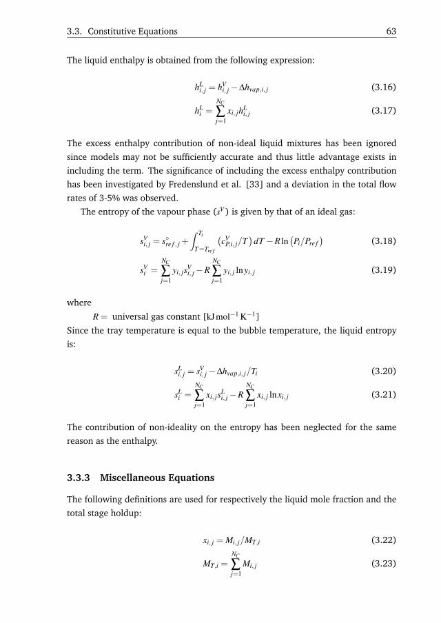
3.3. Constitutive Equations 63
The liquid enthalpy is obtained from the following expression:
hLi, j = hV
i, j−∆hvap,i, j (3.16)
hLi =
NC
∑j=1
xi, jhLi, j (3.17)
The excess enthalpy contribution of non-ideal liquid mixtures has been ignored
since models may not be sufficiently accurate and thus little advantage exists in
including the term. The significance of including the excess enthalpy contribution
has been investigated by Fredenslund et al. [33] and a deviation in the total flow
rates of 3-5% was observed.
The entropy of the vapour phase (sV ) is given by that of an ideal gas:
sVi, j = s◦re f , j +
∫ Ti
T=Tre f
(cV
P,i, j/T)
dT −R ln(Pi/Pre f
)(3.18)
sVi =
NC
∑j=1
yi, jsVi, j−R
NC
∑j=1
yi, j lnyi, j (3.19)
where
R = universal gas constant [kJmol−1 K−1]
Since the tray temperature is equal to the bubble temperature, the liquid entropy
is:
sLi, j = sV
i, j−∆hvap,i, j/Ti (3.20)
sLi =
NC
∑j=1
xi, jsLi, j−R
NC
∑j=1
xi, j lnxi, j (3.21)
The contribution of non-ideality on the entropy has been neglected for the same
reason as the enthalpy.
3.3.3 Miscellaneous Equations
The following definitions are used for respectively the liquid mole fraction and the
total stage holdup:
xi, j = Mi, j/MT,i (3.22)
MT,i =NC
∑j=1
Mi, j (3.23)

64 Chapter 3. Distillation Column Model
Table 3.1. Paths for state functions starting from reference condition (Tre f ,Pre f ) ofpure substances x0. The mixtures are considered ideal.
Path State Conditions Enthalpy Entropy
Start Gas, elements Tre f ,Pre f , x0 h0re f s0
re f
Isobaric change Gas, pure T,Pre f ,x0 ∫ Tt=Tre f
cVP, jdt
∫ Tt=Tre f
cVP, jt dt
Isothermalchange P
Gas, pure T,P,x0 0 −R ln PPre f
Optional: Con-dense at T,P
Liquid, pure T,P,x0 ∆hvap −∆hvapT
Isothermal andisobaric mixing
Liquid orvapour mix-ture
T,P,x 0 −R∑ j x j lnx j
Average molecular weights (MWi) of the liquid and vapour phases can be calculated
from those of the pure components, as follows:
MW Li =
NC
∑j=1
xi, jMW j (3.24)
MWVi =
NC
∑j=1
yi, jMW j (3.25)
The pure component liquid density is calculated from the DIPPR 105 correlation:
ρLi, j =
MW jA j
B1+(1−Ti/C j)
D j
j
(3.26)
The liquid mixture density (ρLi ) is approximated by the ideal expression by assum-
ing no excess volume:
ρLi = MW i
(NC
∑j=1
xi, jMW i, j/ρLi, j
)−1
(3.27)
Vapour density can be calculated based on the ideal gas expression:
ρVi =
MWVi Pi
ZVi RTi
(3.28)
where
ZVi = compressibility factor [-]
According to its definition, ZVi = 1 for ideal gases.
3.3.4 Internal Heat Transfer
A pair of heat-integrated stages describes the link, which enables heat transfer be-
tween two stages in a column.Consider a column with a total of Nihx internally

3.3. Constitutive Equations 65
heat-integrated pairs, corresponding to 2Nihx heat-integrated stages in the column.
A pair of heat-integrated stages, n, can be represented mathematically as a heat
source stage (r(n)) being paired with a heat sink stage (s(n)). This representation
of the pairing enables a description of complex heat integration arrangements, in-
cluding e.g. a heat source stage being paired with multiple heat sink stages [160]
or a few stages being paired, which are not in the same vertical height [23, 51].
The application of the pair description is shown in Illustration 3.3.
Let n = 1,2, . . . ,Nihx, denote the n’th pair of heat-integrated stages r(n) and s(n).
The heat transfer rate due to heat integration is given by Eq. (3.29):
qs(n) =UihxAihx,n(Tr(n)−Ts(n)), n = 1,2, . . .Nihx
qr(n) =−qs(n) (3.29)
qi = 0, i 6= n
where
Uihx = overall heat transfer coefficient [kWm−2 K−1]
Aihx,n = internal heat transfer area [m2]
The relations between r(n) and s(n) and n can be specified as a matrix on the form
nihx ∈ ZNihx×2 where r(n) is the first column element in row nihx, s(n) is the second
column element in row nihx, and Z denote the natural numbers (positive integers).
An illustration of the indices is provided in Illustration 3.3.
3.3.5 Non-mixing Stage Relations
The non-mixing stage accounts for the compressor/valve stage. The mass and en-
ergy dynamics for the compressor are described in Eq. (3.4)-(3.6), whereas the
throttling is assumed adiabatic and at steady state. The throttled liquid is consid-
ered as superheated until it reaches the stage below. Hence, the following applies
to the liquid phase of the non-mixing stage:
cLk = cL
k−1 (3.30)
MW Lk = MW L
k−1 (3.31)
ρLk = ρ
Lk−1 (3.32)
The pressure of the compressor outlet is related to that of the inlet, by the follow-
ing simplified expression resulting from an isentropic balance for ideal gases (Eq.
(2.1)):
Pk = Pk+1
[ηis
(Tk
Tk+1−1)+1]κk/(κk−1)
(3.33)
where

66 Chapter 3. Distillation Column Model
Illustration 3.3. Indexing for internal heat transfer.
Consider the HIDiC with four heat-integrated stages realised by installing
stabbed-in type heat exchangers into the stripping section by Wakabayashi and
Hasebe [160]. The column separates a multicomponent mixture of mainly C8
and C9 aromatics. This design has 30 stages in the rectifying section and 25
stages in the stripping section. In this work, the condenser in the top, the com-
pressor above the feed stage, and the reboiler in the bottom are counted as
stages and therefore 58 stages constitutes the HIDiC. According to the notation
in this work, the heat integration takes place between stages #2-#37, #2-#47,
#7-#54, and #23-#57 corresponding to R1-S5, R1-S15, R6-S22, and R22-S25
where the R refers to a tray in the rectifying section and S refer to the tray in
the stripping section. According to the suggested notation the paring can be
described by
nihx =
r(1) s(1)r(2) s(2)r(3) s(3)r(4) s(4)
=
2 372 477 54
23 57
.By adopting this representation, the model offers a great flexibility of covering
many types of heat integration such as internal as well as external, and even
condenser/reboiler type integration as these are counted as stages as well.
ηis = isentropic efficiency of compression [-]
κk = isentropic expansion factor, which is given by the ratio of constant pres-
sure and constant volume heat capacities [-]
For ideal gasses, the isentropic expansion factor is:
κk =cV
P,k
cVV,k
=cV
P,k
cVP,k−R
(3.34)
Despite the fact that the constant pressure heat capacity is assumed constant in
the derivation of Eq. (3.33)-(3.34), the temperature dependency is still considered
according to Eq. (3.10).
3.3.6 Tray Hydraulics
The liquid and vapour flow rates must be expressed as functions of the state vari-
ables. In a tray column, liquid is entering a tray from the downcomer and leaving
by flowing over the weir. The liquid flow rate can be described by the Francis weir

3.3. Constitutive Equations 67
formula, which states [168]:
Li =
CL
i ρLi H3/2
oW,i
MW Li
, HoW,i > 0
0, HoW,i ≤ 0
(3.35)
HoW,i = Hcl,i−HW (3.36)
hcl,i =MT,iMW L
i
ρLi Aa,i
(3.37)
where
CLi = a constant depending on the liquid loading of the individual trays
[m1.5 s−1]
Aa,i = active area of tray covered by the liquid phase [m2]
HW = weir height [m]
Hcl = clear liquid height (froth ignored) [m]
HoW = liquid height above the weir [m]
Both Aa,i, HW , and CLi are dimensional parameters of the column internals. The
value of CLi is obtained from steady state simulations. A general representation of
a tray in a column with notation is given in Figure 3.3. The different areas of a
tray are listed in Table 3.2. In addition, the table reports typical tray dimensions,
including the relevant tray parameters appearing in Eq. (3.35).
Perforations
Total
Active area
DowncomerPerforations
Weir
Ht
Vapour flow
Liquid flowHW
HL+Ho+Hdc
HgHoW
HS
Dcln
Inlet weir
Outlet weir
Perforations
dh
Liquid flow
Downcomer
Tray
(a) Cross section of a sieve tray.
Perforations
Total
Active area
DowncomerPerforations
Weir
Ht
Vapour flow
Liquid flowHW
HL+Ho+Hdc
HgHoW
HS
Dcln
Inlet weir
Outlet weir
Perforations
dh
Liquid flow
Downcomer
Tray
(b) Notation illustrated on tray.
Figure 3.3. Conventional tray layout.
From the vapour phase, a flow, caused by a pressure gradient, leaves the tray
into the above tray. The vapour flow through perforated trays can be described as

68 Chapter 3. Distillation Column Model
Table 3.2. Definition of regions in a column tray.
Illustration Name Area symbol Comments and sieve traytypical dimensions
Perforations
Total
Active area
DowncomerPerforations
Weir
Ht
Vapour flow
Liquid flowHW
HL+Ho+Hdc
HgHoW
HS
Dcln
Inlet weir
Outlet weir
Perforations
dh
Liquid flow
Downcomer
Tray
Total area AT Column cross sectionalarea. Given by conven-tional sizing methods.
Perforations
Total
Active area
DowncomerPerforations
Weir
Ht
Vapour flow
Liquid flowHW
HL+Ho+Hdc
HgHoW
HS
Dcln
Inlet weir
Outlet weir
Perforations
dh
Liquid flow
Downcomer
Tray
Downcomer are Ad Ad = θdT AT . RoughlyθdT = Ad/AT is in therange 0.1-0.2 [37].
Perforations
Total
Active area
DowncomerPerforations
Weir
Ht
Vapour flow
Liquid flowHW
HL+Ho+Hdc
HgHoW
HS
Dcln
Inlet weir
Outlet weir
Perforations
dh
Liquid flow
Downcomer
Tray
Tray area At At = (1−θdT )AT
Perforations
Total
Active area
DowncomerPerforations
Weir
Ht
Vapour flow
Liquid flowHW
HL+Ho+Hdc
HgHoW
HS
Dcln
Inlet weir
Outlet weir
Perforations
dh
Liquid flow
Downcomer
TrayActive area Aa Aa = (1−2θdT )AT
Perforations
Total
Active area
DowncomerPerforations
Weir
Ht
Vapour flow
Liquid flowHW
HL+Ho+Hdc
HgHoW
HS
Dcln
Inlet weir
Outlet weir
Perforations
dh
Liquid flow
Downcomer
Tray
Perforations area Ap Holes 6.35-12.7 mm di-ameter, θpa = Ap/Aa =0.1 [57]
done by Kolodzie and van Winkle [88]. In this work, the volumetric flow rate is
simplified to be proportional to the square root of the pressure gradient in terms of
liquid height:
Vi = sgn(∆Pi)10−3/2CV
i (ρVi )
0.5
MWVi
|∆Pi|0.5 (3.38)
∆Pi = Pi−Pi−1
where
CVi = a constant depending on the vapour loading (Note that the conversion
factor 10−3/2 appears when kPa is used for pressure) [m2]
g = gravitational acceleration [ms−2]
The operator sgn returns the sign of the pressure driving force, thereby providing
the direction of the vapour flow. In addition, the change in density was neglected
such that a mean density is obtained in Eq. 3.38. This mean density is assumed to
be the density of the vapour in stage i.

3.4. Performance Indicators 69
3.4 Performance Indicators
In this section a set of performance indicators with expressions for evaluating dis-
tillation columns are provided. Suitable expressions for conventional equipment
have been carefully identified and employed for estimation of investment cost of
the new equipment present in e.g. the HIDiC (internal heat transfer equipment).
Note that the models of the performance indicators are independent of the physical
model given in the previous sections. The simulation results obtained by the phys-
ical model are input to the performance indicator models. Therefore, there will be
distinguished between model parameters and economic parameters.
3.4.1 Second-law Efficiency
The second-law efficiency, η2nd , provides insights into the column energy efficiency
and is given by [31]:
η2nd =Wmin
Wlost +Wmin(3.39)
Wmin =NS
∑i=1
(UibL
i |T=Tσ+WibV
i |T=Tσ−FibF,i|T=Tσ
)Wlost =
NS
∑i=1
(UibL
i +WibVi −FibF,i +Qi(1−Tσ/Ts,i)+Ei
)bL
i = hLi −Tσ sL
i
bVi = hV
i −Tσ sVi
bF,i = hF,i−Tσ sF,i
where
Wmin = minimum, isothermal work [kW]
Wlost = lost work [kW]
bi = availability function [kJmol−1]
Tσ = temperature of the surroundings [K]
Ts,i = temperature of the energy sink or source [K]
The internal heat transfer (qi) does not appear in Eq. (3.39) and hence it is distin-
guished from the external heat transfer rate (Qi).
3.4.2 Operating and Capital Expenditures
One method to estimate the capital expenditures (CAPEX) is Guthrie’s Modular
Method as described by e.g. Biegler et al. [9]. This method reflects the me-
dian of equipment cost data, which have deviations of up to 20% for some units.

70 Chapter 3. Distillation Column Model
The CAPEX calculation consists of a summation of the updated bare module costs
(UBMC) corresponding to vessels, trays, heat exchangers, and compressors (see
following sections):
CAPEX = ∑i modules
UBMCi (3.40)
The updated bare module cost (UBMC) is given by the expression:
UBMC = (UF)(BC)(MPF+MF−1) (3.41)
where
UF = update factor (UF=(CE PCI)/115) [-]
BC = base cost [$]
MPF = material and pressure factor [-]
MF = module factor [-]
The estimation of the updated bare module cost is based on empirical correlations
of direct cost of equipment taking historical data into account. The annual index of
the chemical engineering plant cost index is taken from Chemical Engineering Plant
Cost Index (CE PCI) [1] and the value from 2012 is 584.6. The MPF is the material
and pressure factor, which accounts for operating conditions and construction ma-
terial of the individual equipment. The module factor (MF) accounts for direct and
indirect costs (equipment cost, installation, shipping, taxes, and supervision) in a
simple manner. It depends on the bare module cost:
MF =
MF2, BC < 200,000MF4, 200,000≤ BC < 400,000MF6, 400,000≤ BC < 600,000MF8, 600,000≤ BC < 800,000
MF10, 800,000≤ BC < 1,000,000
(3.42)
The values for MF2, MF4, MF6, MF8, and MF10 for the different types of equipment
are reported by Biegler et al. [9].
The operating expenditures (OPEX) is estimated based on the contributions of
the individual equipment:
OPEX = ∑i modules
OCi (3.43)
where
OC= operating cost [$s−1]
The estimation of the contributions on CAPEX and OPEX in terms of UBMC and OC,
respectively, are described in the following sections.

3.4. Performance Indicators 71
3.4.2.1 Column
The distillation column itself consists of a vessel module and a tray stack module.
Only tray columns are considered. Given a steady state column simulation, the
algorithm for sizing and costing is as follows:
1. Provide vapour flow profile Vi and liquid flow profile Li for all trays i
2. Retrieve physical properties MW Li , MWV
i , ρLi , ρV
i , and σLi for all trays i
3. Select tray spacing (HS), downcomer area per total tray area (θdT ), and
flooding factor (FF). Typical values for sieve trays: θdt = 0.10 (Table 3.2),
FF = 0.80, and HS = 609.6mm (24") [9].
4. Determine column diameter
a) Calculate Flv,i =LiMW L
i
ViMWVi
(ρV
i
ρLi
)0.5
b) Read Souders and Brown factor (Csb) from Figure C.1 in Appendix C
c) Calculate the linear vapour velocity un f ,i = Csb
(ρL
i −ρVi
ρVi
)0.5(σL
iσref
)0.2
with σref = 0.020Ns.
d) Calculate the total tray area AT,i =ViMWV
i
εun f FFρVi
, where ε = 0.75 is the area
available for vapour flow. Any correction factor [57] to the vapour ve-
locity is neglected
e) Calculate the column diameter di = (4AT,i/π)0.5
f) Select largest diameter for cost estimation dmax = maxi
di for i trays
5. Calculate UBMC for tray stack
a) Calculate the number of trays NT =NS−Ncpr−Ncnd−Nrbl , where Ncnd = 1is the number of condensers, Nrbl = 1 is the number of reboilers, and Nrbl
is the number of compressors.
b) The tray stack height is calculated based on the tray spacing according
to Htray stack =NT HS
ηtraywhere NT is the number of trays and ηtray is the tray
efficiency.
c) Calculate BCtray stack = 125H0.97tray stackd1.45
max
d) Calculate UBMC using Eq. (3.41) and appropriate MF and MPF
6. Calculate UBMC for column
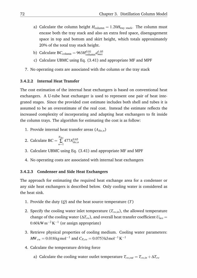
72 Chapter 3. Distillation Column Model
a) Calculate the column height Hcolumn = 1.20Htray stack. The column must
encase both the tray stack and also an extra feed space, disengagement
space in top and bottom and skirt height, which totals approximately
20% of the total tray stack height.
b) Calculate BCcolumn = 963H0.81columnd1.05
max
c) Calculate UBMC using Eq. (3.41) and appropriate MF and MPF
7. No operating costs are associated with the column or the tray stack
3.4.2.2 Internal Heat Transfer
The cost estimation of the internal heat exchangers is based on conventional heat
exchangers. A U-tube heat exchanger is used to represent one pair of heat inte-
grated stages. Since the provided cost estimate includes both shell and tubes it is
assumed to be an overestimate of the real cost. Instead the estimate reflects the
increased complexity of incorporating and adapting heat exchangers to fit inside
the column trays. The algorithm for estimating the cost is as follow:
1. Provide internal heat transfer areas (Aihx,n)
2. Calculate BC =Nihx∑
n=1477A0.65
ihx,n
3. Calculate UBMC using Eq. (3.41) and appropriate MF and MPF
4. No operating costs are associated with internal heat exchangers
3.4.2.3 Condenser and Side Heat Exchangers
The approach for estimating the required heat exchange area for a condenser or
any side heat exchangers is described below. Only cooling water is considered as
the heat sink.
1. Provide the duty (Q) and the heat source temperature (T )
2. Specify the cooling water inlet temperature (Tcw,in), the allowed temperature
change of the cooling water (∆Tcw), and overall heat transfer coefficient Uhex =
0.60kWm−2 K−1 (or assign appropriate)
3. Retrieve physical properties of cooling medium. Cooling water parameters:
MW cw = 0.018kgmol−1 and CP,cw = 0.0753kJmol−1 K−1
4. Calculate the temperature driving force
a) Calculate the cooling water outlet temperature Tcw,out = Tcw,in +∆Tcw

3.4. Performance Indicators 73
b) Assume that the heat source temperature is constant. Check that Tcw,out ≤T (or reasonable lower than T ) is satisfied, otherwise cooling water can
not be used at the specified Tcw,in
c) Calculate the logarithmic mean temperature difference
∆Tlm =(T −Tcw,out)− (T −Tcw,in)
log(T −Tcw,out)− log(T −Tcw,in)
5. Calculate UBMC
a) The area is thus A =Q
Uhex∆Tlm
b) Calculate BC = 477A0.65
c) Calculate UBMC using Eq. (3.41) and appropriate MF and MPF
6. Calculate operating cost
a) Calculate mass flow rate fcw = MWcwQ
∆TcwCP,cw
b) Calculate operating cost OC = Scw fcw. The cost of cooling water can be
obtained using Eq. (2.8)
3.4.2.4 Reboiler and Side Heat Exchangers
The approach for estimating the required heat exchange area for every condenser or
side heat exchanger using is as follows. Only steam is considered as a heat source.
1. Provide the duty (Q) and the heat sink temperature (T )
2. Specify the minimum temperature driving force ∆T = 10K and overall heat
transfer coefficient U = 1.420kWm−2 K−1 for a reboiler or Uhex = 0.60kWm−2 K−1
for heat exchangers (or assign appropriately)
3. Retrieve physical parameters of steam: Molecular weight MW steam = 0.018kgmol−1
4. Calculate steam condition
a) Calculate the required steam temperature Tsteam = T +∆T
b) Calculate steam saturation pressure from Eq. (3.8)
c) Calculate steam heat of vaporisation from Eq. (3.14)
5. Calculate UBMC
a) The area is thus A =Q
Uhex∆T
b) Calculate BC = 477A0.65

74 Chapter 3. Distillation Column Model
c) Calculate UBMC using Eq. (3.41) and appropriate MF and MPF
6. Calculate operating cost
a) Calculate mass flow rate fsteam = MW steamQ
∆hvap,steam[kgs−1]
b) Calculate operating cost OC = Ssteam fsteam. The cost of steam can be ob-
tained using Eq. (2.7).
3.4.2.5 Compressor
Since the duty of the compressor is given from simulation, no further calculations
are required for sizing. The compressor is assumed to be of centrifugal/motor type.
The investment and operating costs for each compressor are:
1. Provide the duty (E)
2. Specify motor efficiency ηcpr
3. Calculate actual compressor power Eactual = E/ηcpr
4. Calculate UBMC
a) Calculate BC = 831E0.77actual
b) Calculate UBMC using Eq. (3.41) and appropriate MF and MPF
5. Calculate operating cost OC = SelectricityEactual . The cost of electricity can be
obtained using Eq. (2.6).
3.4.3 Hydraulic Feasibility Indicator
The hydraulic feasibility indicator (HFI) is a simple indicator for a concentric col-
umn arrangement that describes whether a specified heat exchange area is feasible
or not. The derivation is based on relatively simple geometric considerations, which
are provided by Gadalla et al. [37]. A numerical example is provided in Illustration
3.4 in order to give an order of magnitude of the potential available heat exchange
area in a tray. The definition of HFI is:
HFI = minn
Aihx,n
AHP,n(3.44)
where
Aihx,n = required/specified heat exchange area of pair n [m2]
AHP,n = available heat exchange area of pair n [m2]
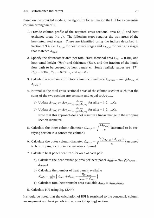
3.4. Performance Indicators 75
Based on the provided models, the algorithm for estimation the HFI for a concentric
column arrangement is:
1. Provide column profile of the required cross sectional area (AT,i) and heat
exchange areas (Aihx,n). The following steps requires the tray areas of the
heat-integrated stages. These are identified using the indices described in
Section 3.3.4, i.e. AT,r(n) for heat source stages and AT,s(n) for heat sink stages
that matches Aihx,n.
2. Specify the downcomer area per total cross sectional area (θdT = 0.10), and
heat panel height (HHP) and thickness (THP), and the fraction of the liquid
flow path to be covered by heat panels ψ. Some realistic values are [37]:
HHP = 0.30m, THP = 0.030m, and ψ = 0.8.
3. Calculate a new concentric total cross sectional area ACT,max = maxn(AT,r(n)+
AT,s(n))
4. Normalise the total cross sectional areas of the column sections such that the
sums of the two sections are constant and equal to ACT,max.
a) Update AT,r(n) := ACT,maxAT,r(n)
AT,r(n)+AT,s(n)for all n = 1,2, . . .Nihx
b) Update AT,s(n) := ACT,maxAT,s(n)
AT,r(n)+AT,s(n)for all n = 1,2, . . .Nihx
Note that this approach does not result in a linear change in the stripping
section diameter.
5. Calculate the inner column diameter dinner,n =
√4AT,r(n)
π(assumed to be rec-
tifying section in a concentric column)
6. Calculate the outer column diameter douter,n =
√4(AT,r(n)+AT,s(n))
π(assumed
to be stripping section in a concentric column)
7. Calculate heat panel heat transfer area of each pair
a) Calculate the heat exchange area per heat panel A1HP = HHPψ(douter,n−dinner,n)
b) Calculate the number of heat panels available
NHP,n =π
2THP
(douter +dinner−
θdtd2outer
douter−dinner
)c) Calculate total heat transfer area available AHP,n = A1HP,nNHP,n
8. Calculate HFI using Eq. (3.44)
It should be noted that the calculation of HFI is restricted to the concentric column
arrangement and heat panels in the outer (stripping) section.

76 Chapter 3. Distillation Column Model
3.5 Model Implementation
The model work flow is summarised in Figure 3.4. Steps 1-9 concern steady state
simulations and Steps 10-12 concern dynamic simulations. The figure illustrates
the progress of the steps for implementation depending on the simulation task pur-
pose, i.e. whether it is static or dynamic. Steps 1–2 are conventional steps for
separation by distillation where Step 3 requires user input for specifying the par-
ticular configuration of interest. This is addressed in more details in Section 3.5.1.
In Step 4, a column design must be selected. A suitable design method is proposed
in Chapter 4. Step 5 serves as an evaluation of the choice of thermodynamic mod-
els based on the selected operating pressures. Steps 6–7 result in a steady state
solution. The purpose of Step 6 is to significantly improve the convergence rate
by providing an initial guess for the solver in Step 7. An extension of the Wang-
Henke Boiling-point (BP) method is used in Step 6. The fsolve function in Matlab
was adopted to simultaneously solve all model equations, design specifications and
separation specifications. Section 3.4 provides a basis for evaluating a distillation
column design for Step 8, where graphical representations such as an xy-diagram
and/or xy-enthalpy diagram can be useful for evaluating the simulation results. If
dynamic simulations are required, one has to proceed to Steps 10–12, beginning
in Step 10 with fixing hydraulic parameters appearing in Eqs. (3.35) and (3.38).
The required dynamic parameters cover for example the active tray area(s) and the
weir height. These parameters are converted to the proportionality constants in the
mentioned equations in Step 10 such that dynamic simulations can be carried out
in Step 11. Detailed considerations on the model parameters, the model implemen-
tation and the model solution procedure are outlined in the following subsections.

3.5. Model Implementation 77
1. Separationformulation Database
2. Select VLE modelsand initialise database
3. Select configuration
4. Select/specifydesign variables
5. VLE assumption ok?
6. Steady state startingguess by ext. BP Method
7. Rigorous simula-tion by simultaneous
correction method
8. Design evaluation
Graphical representation
Performance indicators9. Reasonable design?
10. Design col-umn internals
11. Compute dy-namic parametersfrom steady state
12. Dynamic simulation
Open-loop analysis
Closed-loop analysis
yes
no
yes
no
Figure 3.4. Overview of the workflow required in different simulation studies.

78 Chapter 3. Distillation Column Model
3.5.1 Configuration Parameters
The proposed model framework offers a great flexibility with respect to the selection
of distillation configurations, and ultimately a generalised foundation for compar-
isons. The four configurations introduced in Figure 3.1 can be represented using
the guidelines of parameter selection in Table 3.3. Take for example the MVRC
for which the position of the compressor/valve stage must be at stage 2, whereas
for the HIDiC, the compressor must located above the feed stage. Other positions
of the compressor can also be modelled for the exploration of new configurations.
Furthermore, the framework enables studies, which incorporate for example addi-
tional compressors to cope with separations having complex column temperature
profiles or for higher energy utilisation. For example, the SRVC is conceptually a
combination of the MVRC and the HIDiC. A more detailed example on choosing the
configurations parameters is given in Illustration 3.5.
Table 3.3. Characterisation of the three heat-integrated configurations.
PositionSet Index
Index range
size name MVRC HIDiC SRVC
Compressor/valve Ncpr k 2 k = NF −1 CombinedHeat integratedstages in rectify-ing section
Nihx r 1 1≤ r ≤ NF −1, r 6= k HIDiCandMVRC
Heat integratedstages in strip-ping section
Nihx s NS NF ≤ s≤ NS, s 6= k
3.5.2 Proposed Specifications
The type and the number of the required specifications (i.e. degrees of freedom)
depends on the purpose of the study to be carried out. In the general case (con-
sidering the control volumes in Figure 3.2), a distillation column is fully specified
when the variables listed in Table 3.4 are supplied. However, various combina-
tions of specifications can by supplied in order to eliminate the degrees of freedom.
The link between these, i.e. between the proposed specifications and the degrees
of freedom, is provided in the table. Furthermore, remarks on the link between
the degrees of freedom associated with conventional distillation columns and the
considered heat-integrated distillation configurations are provided.
The dynamic model contains additional parameters compared to simpler ap-
proaches [60]. This is a result of maintaining the energy balances in a dynamic

3.5. Model Implementation 79
Table 3.4. Degrees of freedom analysis for the general distillation column repre-sentation constituted by the stages in Figure 3.2. The mentioned steps refer to themodel workflow in Figure 3.4.
Degree of freedom Remark
Number of stages(NS)
This variable is essential as it influences the total num-ber of degrees of freedom. It is specified in Step 4.
Feed flow rate (Fi) The feed flow rate is specified in Step 1. The in-teger variable NF is introduced to impose constraintsFi = 0, i 6= NF . NF is specified in Step 4. Conceptually, itis possible to increase the number of feed stages but itis not considered in this work.
Feed composition(zi, j)
The same as the feed flow rate applies to the feed com-position. However, the number of degrees of freedom isNS(NC−1) before introducing NF .
Feed Pressure (PF) The same as the feed flow rate applies to the feed pres-sure.
Feed enthalpy (hF) The same as the feed flow rate applies to the feed en-thalpy.
Liquid side drawflow rate (Ui)
In this work, no liquid side draws on the trays are con-sidered. However, the distillate and the bottom productstreams are considered as liquid side draws. This im-plies that Ui = 0, i 6= {1,NS}. It is common to imposepurity constraints, thereby eliminating the degrees offreedom U1 and UNS . As a result, all Ui is typically fixedin Step 1.
Vapour side drawflow rate (Wi)
No vapour side draws are considered in this work. How-ever, this variable is relevant if, for example, a partialcondenser is employed.
Pressure (Pi) In order to consume the thermodynamic degrees of free-dom, the pressure must be specified. The specificationof pressure is a design decision covered in Step 4. Animportant remark, is that the specification of the columnpressure profile also consumes the degrees of freedomassociated of the non-mixing stages (i.e. the compres-sor duty Ek). This is because the constraint of isentropiccompression is imposed in Eq. (3.33).
Internal heat trans-fer rate (qi)
The matrix nihx is obtained through Steps 3-4. Thenqi can either be specified directly or obtained by Eq.(3.29).
form, i.e. expressed in terms of time derivatives rather than using a pseudo-steady
state approximation. The reason for this is to maintain a system of ordinary dif-
ferential equations (ODE) rather than a system of differential-algebraic equations
(DAE), which is computationally more complex to solve.

80 Chapter 3. Distillation Column Model
An advantage of the model is that it accounts for the liquid holdup present both
below and over the weir in a tray. Furthermore, the model accounts for dynamic
tray pressure drops. As a result of these two considerations, the model enables stud-
ies of entrainment flooding and weeping. This is of particular interest in relation
to heat-integrated trays because the liquid and vapour loadings vary significantly
throughout a heat-integrated distillation column. However, for more general dy-
namic studies, the additional model parameters can also represent a disadvantage
in the sense that the model contains more parameters with physical meaning (e.g.
weir height and active tray area). Such parameters are bound within reasonable/re-
alistic limits, which has to be taken into account.
A list of recommendations for fixing these parameters is compiled in Table 3.5.
For liquid and vapour hydraulics, it is suggested to specify the driving forces. Note
that the specification of the dynamic parameters relies on the steady state solution.
Furthermore, note that dynamic simulations can only be performed if tray pressure
drops are non-zero.
Table 3.5. Recommendation for selection of the dynamic column design parametersbased on a steady state simulation. Ncnd is the number of condensers (0 or 1), andNrbl is the number of reboilers (0 or 1).
Variable Appearingin Eq.
Number of Appearance Recommended constraint
CLi (3.35) NS−Ncnd−Nrbl−Ncpr Fix height over weir (HoW,i)
as e.g. 20% of weir height,i.e. HoW,i = 0.2HW
CVi (3.38) NS−Ncnd−Ncpr Fix tray pressure drop ∆Pi as
e.g. 0.70 kPaAa,i (3.35) NS−Ncnd−Nrbl−Ncpr Use conventional column
sizing method (Section3.4.2.1) for AT,i, and cal-culate Aa,i = (1 − 2θdT )AT,iusing e.g. θdT = 0.10
MT,cnd andMT,rbl
(3.1)-(3.2)
Ncnd +Nrbl Fix time constant definedas total holdup divided bysteady state throughput, e.g.5 min
MT,k (com-pressor/-valve)
(3.4)-(3.6)
Ncpr Fix time constant definedas total holdup divided bysteady state throughput, e.g.10 s

3.5. Model Implementation 81
3.5.3 Implementation
The calculation sequence of the model equations is based on the framework pro-
vided by Gani et al. [42]. The set of model equations is decomposed into smaller
subsets that can be solved sequentially and independently of one another as illus-
trated in Figure 3.5. As a result, the dynamic model can be solved as a system of
Subset 1: Thermodynamics1. Obtain states M and T2. x = f (M) [Eq. (3.22)]3. P = f (T,x) [Eq. (3.9), (3.33)]4. y = f (T,P,x) [Eq. (3.7)]
Pure compo-nent and binary
interactionparameters
Subset 2: Physical properties1. ρL = f (T,x) and ρV = f (T,P) [Eq. (3.27)-(3.28)]2. hL = f (T,x) and hV = f (T,y) [Eq. (3.17),(3.13)]3. MW L = f (x) and MWV = f (y) [Eq. (3.24)-(3.25)]
Subset 3: Hydraulics1. L = f (M,ρL,MW L) [Eq. (3.35)]2. V = f (M,ρV ,MWV ,∆P) [Eq. (3.38)]
Subset 4: Couplings1. q = f (T ) [Eq. (3.29)]2. Others, e.g. control loops
Subset 5: Conservation equations1. dM
dt = f (L,x,V,y,F,z) [Eq. (3.1),(3.4)]2. dT
dt = f (L,x,V,y,F,z,Q,q,E,hL,hV ) [Eq. (3.2),(3.6)]
Columndinemsionalparameters
Figure 3.5. Implementation sequence to obtain a system of ordinary differentialequations in the case of ideal vapour phases.
coupled, ordinary differential equations if vapours are considered ideal and when
deviation from non-ideality of the liquid phase is described as a function of liq-
uid phase state variables temperature and composition. When non-ideality of the
vapour phase is the case, a differential-algebraic equation solver (DAE) must be
used, which increases the complexity of the solution procedure. One might argue
that the HIDiC has a main application in the low-to-medium pressure range since
the pressure elevation is often minimised to reduce both the OPEX and the CAPEX
associated with the compressor. The full model is implemented in Matlab and will
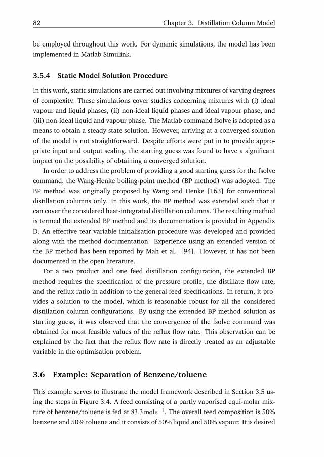
82 Chapter 3. Distillation Column Model
be employed throughout this work. For dynamic simulations, the model has been
implemented in Matlab Simulink.
3.5.4 Static Model Solution Procedure
In this work, static simulations are carried out involving mixtures of varying degrees
of complexity. These simulations cover studies concerning mixtures with (i) ideal
vapour and liquid phases, (ii) non-ideal liquid phases and ideal vapour phase, and
(iii) non-ideal liquid and vapour phase. The Matlab command fsolve is adopted as a
means to obtain a steady state solution. However, arriving at a converged solution
of the model is not straightforward. Despite efforts were put in to provide appro-
priate input and output scaling, the starting guess was found to have a significant
impact on the possibility of obtaining a converged solution.
In order to address the problem of providing a good starting guess for the fsolve
command, the Wang-Henke boiling-point method (BP method) was adopted. The
BP method was originally proposed by Wang and Henke [163] for conventional
distillation columns only. In this work, the BP method was extended such that it
can cover the considered heat-integrated distillation columns. The resulting method
is termed the extended BP method and its documentation is provided in Appendix
D. An effective tear variable initialisation procedure was developed and provided
along with the method documentation. Experience using an extended version of
the BP method has been reported by Mah et al. [94]. However, it has not been
documented in the open literature.
For a two product and one feed distillation configuration, the extended BP
method requires the specification of the pressure profile, the distillate flow rate,
and the reflux ratio in addition to the general feed specifications. In return, it pro-
vides a solution to the model, which is reasonable robust for all the considered
distillation column configurations. By using the extended BP method solution as
starting guess, it was observed that the convergence of the fsolve command was
obtained for most feasible values of the reflux flow rate. This observation can be
explained by the fact that the reflux flow rate is directly treated as an adjustable
variable in the optimisation problem.
3.6 Example: Separation of Benzene/toluene
This example serves to illustrate the model framework described in Section 3.5 us-
ing the steps in Figure 3.4. A feed consisting of a partly vaporised equi-molar mix-
ture of benzene/toluene is fed at 83.3 mols−1. The overall feed composition is 50%
benzene and 50% toluene and it consists of 50% liquid and 50% vapour. It is desired

3.6. Example: Separation of Benzene/toluene 83
to produce 99.5% pure benzene in the top and 99.5% pure toluene in the bottom.
These specifications complete Step 1 (Figure 3.4) and thus the database must be
accessed for pure component and mixture properties. The benzene/toluene mix-
ture can be described satisfactorily using the assumption of ideal liquid and vapour
phases in Step 2, and the HIDiC is chosen as the considered configuration in Step
3. In Step 4, the design is provided by Nakaiwa et al. [111]: An operating pressure
in the feed stage of 101.3 kPa, a compression ratio of 2.553, an overall heat transfer
coefficient of 0.60 kWm−2 K−1, a heat exchange area 5.0 m2 stage−1, 40 trays in the
rectifying section, and 40 trays in the stripping section. All 40 trays are heat inte-
grated from top to bottom in each section. In terms of stages, the HIDiC consists of
83 stages including all trays and the condenser, reboiler and the compressor/valve.
In this example, an additional tray pressure drop of 0.70 kPa is assumed. The ther-
modynamic models are reasonable in Step 5 for the selected operating conditions.
The resulting model has 249 states and 421 equations to be solved simultaneously.
The following additional input were provided for the extended BP method: The dis-
tillate flow rate, which can be calculated from overall mass balance D = 41.7mols−1
and a reflux ratio initial estimate RR = 0.5. Convergence of a steady state solution
is obtained after 47 iterations and it proceeds according to Figure 3.6. As the tem-
perature profile is among the tear variables its convergence is also shown in Figure
3.6.
0 20 4010−9
10−7
10−5
10−3
10−1
101
103
TOL=10−8
Iteration
Erro
r
0 20 40384
386
388
390
392
394
396
398
TOL=10−8
Iteration
Tem
pera
ture
[K]
T2TNcpr
TNS−1
Figure 3.6. Convergence plot of error and selected tear variables.
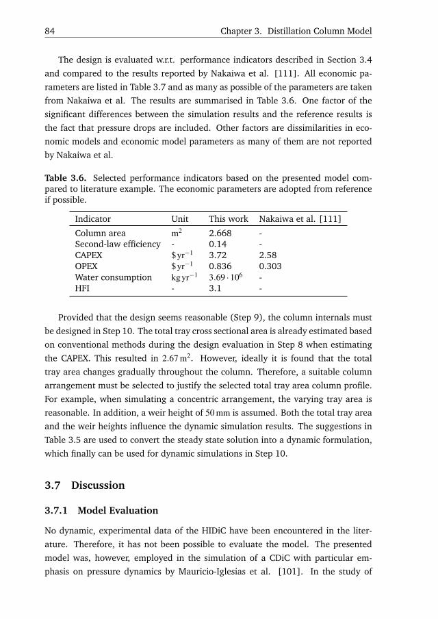
84 Chapter 3. Distillation Column Model
The design is evaluated w.r.t. performance indicators described in Section 3.4
and compared to the results reported by Nakaiwa et al. [111]. All economic pa-
rameters are listed in Table 3.7 and as many as possible of the parameters are taken
from Nakaiwa et al. The results are summarised in Table 3.6. One factor of the
significant differences between the simulation results and the reference results is
the fact that pressure drops are included. Other factors are dissimilarities in eco-
nomic models and economic model parameters as many of them are not reported
by Nakaiwa et al.
Table 3.6. Selected performance indicators based on the presented model com-pared to literature example. The economic parameters are adopted from referenceif possible.
Indicator Unit This work Nakaiwa et al. [111]
Column area m2 2.668 -Second-law efficiency - 0.14 -CAPEX $yr−1 3.72 2.58OPEX $yr−1 0.836 0.303Water consumption kgyr−1 3.69 ·106 -HFI - 3.1 -
Provided that the design seems reasonable (Step 9), the column internals must
be designed in Step 10. The total tray cross sectional area is already estimated based
on conventional methods during the design evaluation in Step 8 when estimating
the CAPEX. This resulted in 2.67 m2. However, ideally it is found that the total
tray area changes gradually throughout the column. Therefore, a suitable column
arrangement must be selected to justify the selected total tray area column profile.
For example, when simulating a concentric arrangement, the varying tray area is
reasonable. In addition, a weir height of 50 mm is assumed. Both the total tray area
and the weir heights influence the dynamic simulation results. The suggestions in
Table 3.5 are used to convert the steady state solution into a dynamic formulation,
which finally can be used for dynamic simulations in Step 10.
3.7 Discussion
3.7.1 Model Evaluation
No dynamic, experimental data of the HIDiC have been encountered in the liter-
ature. Therefore, it has not been possible to evaluate the model. The presented
model was, however, employed in the simulation of a CDiC with particular em-
phasis on pressure dynamics by Mauricio-Iglesias et al. [101]. In the study of

3.7. Discussion 85
Table 3.7. Economic parameters for performance indicators. The parameters aregrouped in column parameters, which has impact on the model itself, and economicparameters, which has only impact on the performance indicators (see Section 3.4).
Class Parameter Unit Value
Column parametersInternal heatexchanger
Heat transfer coefficient kWm−2 K−1 0.60
Heat exchange area m2 5Tray Active area per tray area - 0.70
Weir height m 0.05Weir overfill fraction - 0.20Pressure drop kPa 0.70
Condenser Time constant min 5Reboiler Time constant min 5Compressor Isentropic efficiency - 0.80
Time constant s 10
Economic parametersGeneral Electricity price $kWh−1 0.0843
Steam $t−1 16.8634Cooling water (at 300 K) $t−1 0.0590Year - 2012Project life time yr 5Service factor - 1Materials - Carbon steel
Tray Efficiency - 1Flooding factor - 0.80Void fraction - 0.75Type - SieveSpacing mm 609.60 (24")
Condenser Water temperature in-crease
K 5.0
Heat transfer coefficient kWm−2 K−1 0.60Type - Floating head
Reboiler Heat transfer coefficient kWm−2 K−1 1.420Type - Kettle reboiler
Compressor Motor efficiency - 0.90Type - Centrifugal/ mo-
tor
Mauricio-Iglesias et al., the implications of different control structures for control-
ling the column pressure were assessed by simulations. The simulation results were
benchmarked against experimental results of an industrial distillation column sep-
arating a mixture of 2-propanol/water azeotrope. Mauricio-Iglesias et al. [101]
concluded, that the model could satisfactorily account for the pressure dynamics

86 Chapter 3. Distillation Column Model
in relation to the considered separation. Based on this experience, it is assumed
that the presented model provides a reasonable representation of a heat-integrated
distillation column. However, it is expected that the pressure dynamics play a more
important role in the HIDiC due to the strong interactions with the internal heat
transfer.
3.7.2 Internals Limitation
One significant limitation of the presented model is that it is based on equilibrium-
stages, resembling those in tray columns. In certain separations, packed column
internals are preferred, e.g. in the structured plate HIDiC [19]. Modelling of these
configurations requires alternative, rate-based approaches. However, for bench-
marking studies without further detailed information on the layout of the column
internals, it is reasonable to consider tray columns. In addition, equilibrium-based
models are typically preferred because of fewer required model parameters.
3.7.3 Economic Models
As mentioned in the benchmarking case study, the evaluation of the techno-economic
feasibility of the HIDiC is not a straightforward task. In fact, great uncertainty is
associated with this task. Since the HIDiC was introduced in 1977 [94] a major con-
cern has been to demonstrate the benefit w.r.t. energy consumption compared to
conventional distillation by either comparing utility consumptions or second-law ef-
ficiencies. A more direct measure of the economic feasibility is total annualised cost
(TAC). TAC calculation, however, relies heavily on the selected economic model.
Typically the installation of internal heat exchangers and a compressor appear to
be the major expenses in the HIDiC. Hence, the costing procedures of these units,
e.g. selection of types of internal heat exchangers will have a significant impact
on the TAC. Some authors [111, 158] add an additional penalty in the magnitude
of 20-50% on the HIDiC capital expenditures to account for increased complexity
of the column layout. It is thus vital, that more research is carried out in order to
improve the accuracy of the costing procedure of the HIDiC. Furthermore, the es-
timation of operation expenditures depends upon the utility prices and availability.
For example, steam prices might be significantly lower if steam is present in excess
in the process or at neighbouring facilities. Hence, it is essential to employ identical
costing scenarios in benchmark studies, which is made possible within the provided
framework. It should be noted, that the installation of internal heat transfer does
not only affect the economic feasibility but also the technical feasibility since these
might reduce the separation performance. Many of the economic and technical
3.8. Conclusion 87
feasibility aspects are covered in Chapter 5.
Two distinct uncertainties are expected in the economic models presented in
Section 3.4: Estimation of the bare module cost of (i) an internal heat exchanger
and (ii) the column. A conventional shell-and-tube heat exchanger economic model
is used for (i), which means that the module cost accounts for both the shell and the
tubes. To realise internal heat transfer in a real HIDiC, it is unlikely that the heat
exchanger shell is required. Furthermore, simpler layouts of the internal heat ex-
changers (e.g. heat panels) are proposed in the literature. Both arguments suggest
that the presented economic model gives rise to conservative estimates (overes-
timates) of the internal heat exchanger bare module costs. For the column bare
module cost (including the tray stack), one single tower having the widest diame-
ter and the maximum pressure among all the trays is assumed. This approach does
not restrict the bare module cost estimation to certain column arrangements, since
a wide selection of arrangements is proposed in literature (see Table 2.5). This
assumption might lead to a bare module cost estimate, which is smaller than the
case where the column is physically divided in the two column sections. But as
the required column diameter is gradually changing in e.g. the concentric HIDiC,
using the maximum column diameter is assumed to compensate for the above cost
underestimate.
3.8 Conclusion
A generic distillation column model is presented and demonstrated. It can describe
both adiabatic and diabatic distillation columns covering among others the conven-
tional, the heat-integrated, and the mechanical vapour recompression distillation
column. In addition, the framework offers the flexibility of expanding the current
existing configuration library due to the generic structure. The model is embed-
ded in a framework enabling studies to gain insights into e.g. static properties and
the dynamic behaviours in a consistent manner. A Matlab simulation platform was
developed containing a full implementation of the model and a database of the
different configurations and pure component and mixture properties. A solution
algorithm was developed in order to obtain robust convergence of the model.

88 Chapter 3. Distillation Column Model
Illustration 3.4. Derivation and estimation of the available tray heat transfer
area given the tray dimensions [37].
The heat panels are assumed to be placed on the outside of the wall of the inner
tube in the concentric arrangement according to the figure below:
σ
σ
dinner douter
Lδ
T
The area of one heat panel is
A1HP = 2LHHP,
where HHP is the height. The areas associated with the thickness of the panels
are ignored. In this work, an additional parameter ψ is introduced that is defined
as the fraction of liquid flow to be covered by heat panels, i.e. ψ = L/σ . The
number of heat panels
NHP =Linner
T+
Louter−Linner
2T,
where Linner = πdinner − δ is the circumference of the inner tube minus δ and
Louter = πdouter− δ is the circumference of the outer tube minus δ . The down-
comer width is given by δ = Ad/σ = θdT Aouter/σ . The curvatures are ignored
such that the downcomer can be approximated by a rectangle. It is assumed
that no gaps between the heat panels are required on the outer wall of the inner
tube.
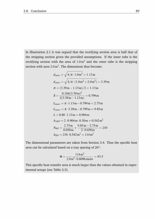
3.8. Conclusion 89
In Illustration 2.1 it was argued that the rectifying section area is half that of
the stripping section given the provided assumptions. If the inner tube is the
rectifying section with the area of 1.0 m2 and the outer tube is the stripping
section with area 2.0 m2. The dimensions thus become:
dinner =
√4/π ·1.0m2 = 1.13m
douter =
√4/π · (1.0m2 +2.0m2) = 3.39m
σ = (3.39m−1.13m)/2 = 1.13m
δ =0.10π(3.39m)2
2(3.39m−1.13m)= 0.799m
Linner = π ·1.13m−0.799m = 2.75m
Louter = π ·3.39m−0.799m = 9.85m
L = 0.80 ·1.13m = 0.904m
A1HP = 2 ·0.904m ·0.30m = 0.542m2
NHP =2.75m
0.030m+
9.85m−2.75m2 ·0.030m
= 210
AHP = 210 ·0.542m2 = 114m2
The dimensional parameters are taken from Section 3.4. Thus the specific heat
area can be calculated based on a tray spacing of 24":
Φ =114m2
2.0m2 ·0.6096metre= 93.5
This specific heat transfer area is much larger than the values obtained in exper-
imental setups (see Table 2.3).

90 Chapter 3. Distillation Column Model
Illustration 3.5. Obtaining an MVRC, a HIDiC, and an SRVC by adjusting
configurations parameters.
Provided a distillation column with nine stages where stage #6 is the feed stage.
The first #1 and the last #9 are respectively condenser and reboiler. According
to Table 3.3, selecting the compressor/valve stage k = 2 and heat integrated
stage in the rectifying section as r = 1 and in the stripping section s = NS = 9the resulting configurations is the MVRC. In order to obtain a HIDiC, the
compressor/valve stage is set to k = NF −1 = 5 and as many trays as possible are
heat integrated, i.e. r = [2,3,4] and s = [6,7,8]. Finally, the SRVC is obtained by
using a combination of the MVRC and the HIDiC although one additional stage
is used as compressor/valve and thus only two stages can be heat-integrated in
each section. The illustration below summarises this example.
#1
#2
#3
#4
#5
#6
#7
#8
#9
#1
#2
#3
#4
#5
#6
#7
#8
#9
#1
#2
#3
#4
#5
#6
#7
#8
#9
#1
#2
#3
#4
#5
#6
#7
#8
#9
Heat source Heat sink
Compressor/valve stage Stage
CDiC MVRC HIDiC SRVC
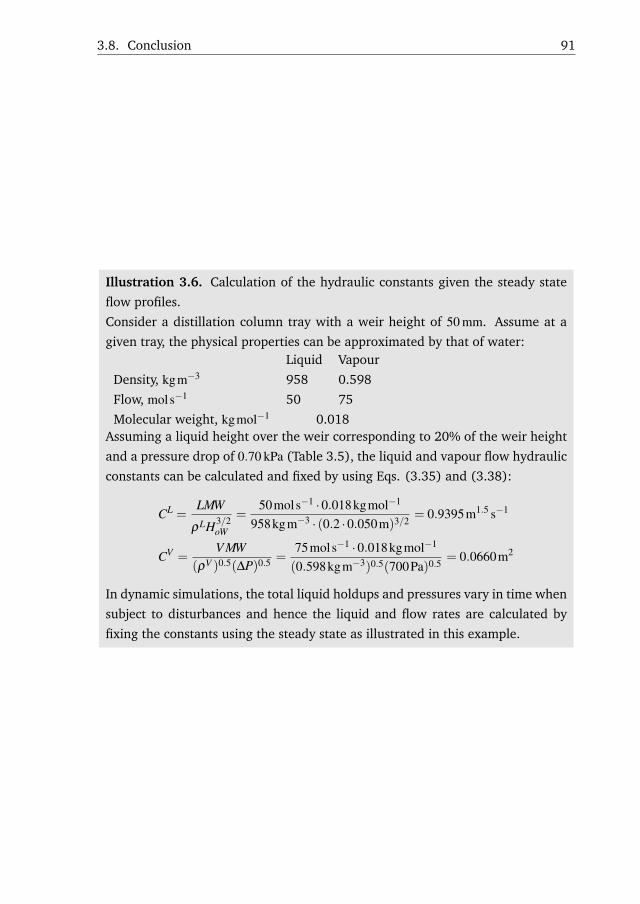
3.8. Conclusion 91
Illustration 3.6. Calculation of the hydraulic constants given the steady state
flow profiles.
Consider a distillation column tray with a weir height of 50 mm. Assume at a
given tray, the physical properties can be approximated by that of water:Liquid Vapour
Density, kgm−3 958 0.598
Flow, mols−1 50 75
Molecular weight, kgmol−1 0.018Assuming a liquid height over the weir corresponding to 20% of the weir height
and a pressure drop of 0.70 kPa (Table 3.5), the liquid and vapour flow hydraulic
constants can be calculated and fixed by using Eqs. (3.35) and (3.38):
CL =LMW
ρLH3/2oW
=50mols−1 ·0.018kgmol−1
958kgm−3 · (0.2 ·0.050m)3/2= 0.9395m1.5 s−1
CV =V MW
(ρV )0.5(∆P)0.5 =75mols−1 ·0.018kgmol−1
(0.598kgm−3)0.5(700Pa)0.5= 0.0660m2
In dynamic simulations, the total liquid holdups and pressures vary in time when
subject to disturbances and hence the liquid and flow rates are calculated by
fixing the constants using the steady state as illustrated in this example.


Chapter4
Conceptual Design
An iterative design method for the conceptual design of the
mechanical vapour recompression column (MVRC), the heat-
integrated distillation column (HIDiC), and the secondary re-
flux and vaporisation column (SRVC), is presented. The method
is tailor-made for the developed model framework and allows
relatively fast conceptual design of considered configurations
for a given separation (binary or a multicomponent mixture).
An economic objective function is used to direct the progress
of the design towards optimality and a generic distillation col-
umn configuration is used to represent the considered con-
figurations. The method is more intuitive and takes a more
stepwise approach to the design problem, compared to other
superstructure-based MINLP approaches relying on mathemat-
ical programming. However, on present form, a fully optimal
design is not guaranteed.
The application of the design method on the MVRC, the HIDiC,
and the SRVC is outlined. Finally, the method is discussed and
exemplified for a binary mixture of benzene/toluene and a mul-
ticomponent mixture of aromatic compounds.
The design method was presented at the AIChE Annual Meet-
ing 2015 in Salt Lake City, Utah, in a presentation entitled
"Design Methods for the Heat-Integrated Distillation Column
(HIDiC)". Furthermore, an early stage of the design method
was presented at the Distillation and Absorption conference

94 Chapter 4. Conceptual Design
[K. Meyer, L. Ianniciello, J.E. Nielsen, T. Bisgaard, J.K. Huu-
som, and J. Abildskov. Hidic – design, sensitivity and graphical
representation. Proceedings of Distillation and Absorption, pages
727–732, 2014].

4.1. Introduction 95
4.1 Introduction
As a basis for the benchmarking of distillation column configuration alternatives,
a satisfactory design method is required. Furthermore, such a method is essential
for obtaining economically feasible designs for investigating dynamics and control.
Based on the model presented in Chapter 3, a simulation-based design method for
exploring various distillation column configuration alternatives by allowing gradual
conversion between the configurations would be useful. However, existing design
methods can not directly be extended to all the configurations, studied in this the-
sis. Thus, the need for developing the present design algorithm was identified. The
presented design algorithm is a generalisation of the experience gained in simu-
lations of a variety of mixtures taking into account a relative large design space.
Hence, common trends in the resulting optimum designs w.r.t. TAC have been iden-
tified and systematised. Furthermore, the experiences are verified by qualitative
considerations (see Section 4.6).
4.1.1 Configuration Generalisation
The mechanical vapour recompression column (MVRC), the heat-integrated distil-
lation column (HIDiC), and the secondary recompression column (SRVC) are tar-
geted as potential candidates for improvements as alternatives to the conventional
distillation column (CDiC). In the scope of this work, economic improvements are
essential, while reductions in e.g. energy consumption are optional. However,
energy reductions are closely related to economic improvements. A generalised
distillation column structure has been defined, which is capable of describing the
targeted potential candidates (HIDiC, MVRC, and SRVC) and the CDiC. This gen-
eralised distillation column structure is illustrated in Figure 4.1. The considered
configurations in this work are limited to one feed and two product stream separa-
tions, which is reflected in the figure.
4.1.2 Design Reservations
All obtainable designs by the design algorithm are restricted to the four configura-
tions: CDiC, MVRC, HIDiC and SRVC. Additional design reservations are made in
order to reduce the complexity of the design problem. These are listed and moti-
vated below:
• Sequenced heat-integrated trays: It was previously concluded that the con-
centric HIDiC, in particular, is a potential arrangement of the HIDiC for tray
columns. This arrangement limits the pairing to stages of the same vertical

96 Chapter 4. Conceptual Design
CRextCRint
Qcnd
Qrbl
Aint,n
Aint,Nint
Aint,11
D
B
L
V
Aext
ˆ(1)s
ˆ( )ˆs n
intˆ( )s N
ˆ(1)r
ˆ( )ˆr n
intˆ( )r N
NT
ˆF
N
ˆ 1F
N
ˆFN
P
Qvlv,extQvlv,int
Figure 4.1. A generalised distillation column structure indicating the design de-grees of freedom with symbols.
height. Furthermore, no significant additional complexity/investment cost
associated with the installation of heat panels gradually along the height in
the concentric HIDiC is expected. Various authors [23, 142, 51] claim that
the optimal design only contain few pairings with large heat exchange areas.
However, such conclusions are often favoured because of the high CAPEX of
the required heat exchangers when conventional economic models are used.
The economic model of a conventional heat exchanger is typically valid for
a shell-and-tube heat exchange. Clearly, such a model can not accurately de-
scribe the cost of simple heat panels inside a distillation column tray.
• Uniform heat exchange area approach: This approach implies a constant

4.1. Introduction 97
heat exchange area between every pair of heat-integrated trays. An alterna-
tive approach represented in the design literature is the uniform heat transfer
rate approach [41, 154]. However, an optimal approach w.r.t. economy lies
between the two approaches [155]. This conclusion relies again on the eco-
nomic models for the heat exchangers and the column, although no experi-
mental data have confirmed such models. It was previously concluded that
heat panels must be installed in order to achieve sufficient heat transfer area.
Hence, it is argued that the uniform heat exchange area approach reflects a
solution, which is most likely to be realised when using heat panels. In par-
ticular in relation to the reservation of using sequenced heat-integrated trays,
it is presumed that the costs of construction of trays with e.g. heat panels can
be reduced; uniform trays that can be massproduced in modules thus favours
the uniform heat exchange area approach.
• Compression ratio(s): The compression ratio is not considered as a means
to improve the economic performance of a design. The compression ratio is
solely used for achieving the specified minimum temperature driving force(s)
among the paired stages. This is reasonable, as the compressor duty has a
relatively small impact on the total annualised cost [155].
• Economic design approach: Despite the fact that the available economic
models are not properly validated, the total annualised cost (TAC) is em-
ployed as the design objective function. It is important to account for the
existing trade-off between operating costs and investment costs, which the
TAC provides.
• Only tray/tray and condenser/reboiler type heat integration: The allow-
able pairings are restricted to only tray/tray and condenser/reboiler type
heat integration. The argument for this reservation is that tray/condenser or
tray/reboiler type heat integration can be approximated by involving the tray
just below the condenser or above the reboiler rather that the condenser or
reboiler. Condenser/tray type heat integration is encountered in the graphical
design method by Wakabayashi and Hasebe [159].
• Reboiler duty rather than feed preheat duty: The ideal HIDiC has neither a
condenser nor a reboiler duties. However, in order to realise such a configura-
tion, the feed has to be partly vaporised. To obtain this, the feed can either be
preheated or exist on this form prior to the distillation column. Since only the
separations of liquid saturated mixtures are considered in work, a feed pre-
heater or a reboiler is required. During this work, it has been found that the

98 Chapter 4. Conceptual Design
heat input is utilised more efficiently when it is added in the reboiler rather
than to the feed. Therefore, feed preheating is not considered in the method.
4.2 Nomenclature
The design degrees of freedom associated with the generalised column representa-
tion are provided in Figure 3.1. Adopted definitions in this chapter are explained
in the following subsections.
4.2.1 Design Degrees of Freedom
Consider the general two-product distillation column illustrated in Figure 4.1 with
NT trays (i.e. excluding condenser and reboiler) and one feed introduced at stage
NF counted from the top. A bottom product is removed from the reboiler, located
below stage NT at a rate B, while a fraction is vaporised at a rate V and returned
to the bottom stage, denoted by the boil-up ratio (V/B). The external heat duty, re-
quired for vaporising the returned stream, is termed the reboiler duty and denoted
Qrbl . The column section spanning the feed tray to the bottom tray is the stripping
section (abbreviated "str"). The pressure of the feed tray is denoted PNF. The top
vapour of the stripping section is compressed at a compression ratio CRint before it
enters the bottom of the rectifying section (abbreviated "rct"). The pressure in the
bottom tray of the rectifying section is thus CRintPNF. The liquid from the rectifying
section is throttled by a valve before entering the feed stage. The top vapour of
the rectifying section is compressed at a compression ratio CRext before it is con-
densed using an external energy sink with the condenser duty (Qcnd). The distillate
is removed at a rate D from the condenser while the rest of the overhead vapour
stream L is returned to the column top stage consistent with the value of the reflux
ratio (RR = L/D). The possibility of considering valve cooling for the two throttling
valves is addressed by the duties Qvlv,int and Qvlv,ext .
4.2.2 Pairs – Heat-integrated Stages
In order to simplify the nomenclature, there will be distinguished between internal
heat integration and external heat integration. Internal heat integration takes place
between the column trays and external heat integration takes place between the
condenser and the reboiler. Both types of heat integration are described by Eq.
(3.29) but subscripts ("int" and "ext") are used to distinguish between the types
when needed. The influence on the selection of the variables indicated in Figure
4.1 are summarised in Table 4.1. As indicated in the table, a compression ratio of

4.3. Design Method Overview 99
unity is a mathematical indication of the absence of a compression stage. The same
applies to a heat exchanger; a heat exchange area of zero corresponds to absence
of a heat exchanger. Using this representation, the four configurations of Figure 4.1
can be represented.
Table 4.1. Characterisation of different heat-integrated distillation column config-urations.
Configuration Internal heat integration External heat integration
CRint Aint,n CRext Aext
CDiC 1 0 (all) 1 0MVRC 1 0 (all) >1 >0HIDiC >1 >0 0 0SRVC >1 >0 >1 >0
4.2.3 Indexing
It is more convenient to refer to tray numbers instead of stage numbers because
stages describe trays, compressors, condensers and reboilers. The tray basis is there-
fore more intuitive in this context. When a compressor is added/removed during
the design procedure, the stage numbers of certain trays are altered, whereas the
tray numbers remain unchanged. A new set of indices are introduced by adding a
circumflex on the indices introduced in Chapter 3. Hence, the tray number (i) spans
i = 1,2, . . . ,NT . The feed tray is i = NF . Furthermore, the number of heat-integrated
pairs (Nihx) can be partitioned in Nint internal pairings and one external pairing. A
pair of heat-integrated trays, n, can be represented mathematically as a heat source
tray, r(n), being paired with a heat sink tray, s(n). Thus, let n = 1,2, . . . ,Nint , denote
the n’th pair of heat-integrated stages r(n) and s(n). The index n does not cover
the condenser/reboiler type heat integration. The usage of the tray based indices is
illustrated on an SRVC configuration in Illustration 3.3.
4.3 Design Method Overview
The conceptual design algorithm is illustrated in Figure 4.2. An overview is pre-
sented below and the steps are further elaborated in the following section. Step 1
requires the following input: (i) what is to be separated, (ii) the purity demands
of the product stream(s), (iii) a formulation of the objective function that should
direct the design to an optimal solution, and (iv) a minimum temperature driving
force for heat integration. In Step 2, a conceptual design of the CDiC must be es-
tablished by minimising/maximising the specified objective function in Step 1, item

100 Chapter 4. Conceptual Design
Illustration 4.1. Introducing the tray basis notation for the CDiC and the SRVC
from Illustration 3.3.
The tray basis indexing for the simple case of a CDiC and the SRVC is illustrated
below:
Heat source Heat sink
Compressor/valve stage Stage
i
Stage Tray
1
2
3
4
5
6
7
8
9
Basis
i
1
2
3
4
5
6
7
-
-
CDiC
i
Stage Tray
1
2
3
4
5
6
7
8
9
Basis
i
-
1
2
-
3
4
5
-
-
SRVC
As illustrated, the adopted tray basis is visual. When conducting the simulation
required for this method, simple relation are used to convert the tray basis to
stage basis. For example, the total number of stages is NS = NT +Ncnd + 1+ 1,
i.e. the sum of the total number of trays, the number of condensers, and the
number of reboilers. In addition, the feed location NF in stage basis is simply
NF = NF +Ncpr + 1, i.e. the sum of compressors plus one condenser provided
that the compressors are only located above the feed stage.
(iii). In Step 3, the CDiC is converted into one of the considered configurations (Fig-
ure 3.1) by including either or both internal and external heat integration. In the
following step, the remaining design degrees of freedom being the heat exchange
area for each pairing (Step 4a), the total number of trays (Step 4b), and the pairing
arrangement (Step 4c) are adjusted by iteration. In Step 5, column simulations
are repeated as the compression ratio (CR) is adjusted (in Step 6) until a specified

4.4. Detailed Description of the Design Method 101
minimum temperature gradient among the heat-integrated stage(s) is obtained by
iteration. A column simulation means obtaining a converged simulation satisfying
mass and energy balances and specified product purity constraints formulated in
Step 1. In Step 7, the design objective function (specified in Step 1) is calculated
and evaluated in Step 8, if further iterations must be carried out.
1. Problem formulation
2. ConceptualCDiC design
3. Target and configureheat integration type
4. Improve design4a. Adjust A
4b. Adjust NT4c. Configure pairing
5. Converge simulationw.r.t. purity specifications
6. ∆Tmin = ∆Tspec?∆V = 0?
Adjust CRAdjust Qvlv,ext
7. Calculate the de-sign objective, F(k)
ob j
8. ∆F(k)ob j sensitive? Finish
k = 0
yes
no
noyes
k := k+1
Figure 4.2. Conceptual design of a heat-integrated distillation column.
4.4 Detailed Description of the Design Method
This section provides a detailed description of the design method by describing all
the required actions and the tools needed to use the method.
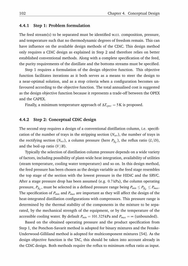
102 Chapter 4. Conceptual Design
4.4.1 Step 1: Problem formulation
The feed stream(s) to be separated must be identified w.r.t. composition, pressure,
and temperature such that no thermodynamic degrees of freedom remain. This can
have influence on the available design methods of the CDiC. This design method
only requires a CDiC design as explained in Step 2 and therefore relies on better
established conventional methods. Along with a complete specification of the feed,
the purity requirements of the distillate and the bottoms streams must be specified.
Step 1 requires a formulation of the design objective function. This objective
function facilitates iterations as it both serves as a means to steer the design to
a near-optimal solution, and as a stop criteria when a configuration becomes un-
favoured according to the objective function. The total annualised cost is suggested
as the design objective function because it represents a trade-off between the OPEX
and the CAPEX.
Finally, a minimum temperature approach of ∆Tspec = 5K is proposed.
4.4.2 Step 2: Conceptual CDiC design
The second step requires a design of a conventional distillation column, i.e. specifi-
cation of the number of trays in the stripping section (Nstr), the number of trays in
the rectifying section (Nrct), a column pressure (here PNF), the reflux ratio (L/D),
and the boil-up ratio (V/B).
Typically the selection of distillation column pressure depends on a wide variety
of factors, including possibility of plant-wide heat integration, availability of utilities
(steam temperature, cooling water temperature) and so on. In this design method,
the feed pressure has been chosen as the design variable as the feed stage resembles
the top stage of the section with the lowest pressure in the HIDiC and the SRVC.
After a stage pressure drop has been assumed (e.g. 0.7 kPa), the column operating
pressure, PNF, must be selected in a defined pressure range being Pmin ≤ PNF
≤ Pmax.
The specification of Pmin and Pmax are important as they will affect the design of the
heat-integrated distillation configurations with compressors. This pressure range is
determined by the thermal stability of the components in the mixture to be sepa-
rated, by the mechanical strength of the equipment, or by the temperature of the
accessible cooling water. By default Pmin = 101.325kPa and Pmax = ∞ (unbounded).
Based on the obtained operating pressure and the product specification from
Step 1, the Ponchon-Savarit method is adopted for binary mixtures and the Fenske-
Underwood-Gilliland method is adopted for multicomponent mixtures [54]. As the
design objective function is the TAC, this should be taken into account already in
the CDiC design. Both methods require the reflux to minimum reflux ratio as input.

4.4. Detailed Description of the Design Method 103
Thus the design is carried out as a one-dimensional optimisation procedure, where
this ratio is manually adjusted until a minimum TAC is obtained. A minimum TAC
is often resulted as CAPEX increases with an increasing number of stages, while the
OPEX decreases as external utility requirements are reduced. In the end of Step 2,
the iteration variable k is initialised as k = 0.
4.4.3 Step 3: Target and configure heat integration type
Two types of heat integration are possible; internal heat integration and external
heat integration. Only one type can be targeted when Step 3 is considered. The
following actions are required, depending on the targeted heat integration type:
• Internal heat integration: This results in the splitting of the two column sec-
tions. A compressor is added to the vapour exiting the stripping section, and
a throttling valve is added to the liquid exiting the rectifying section. By
doing this, additional design degrees of freedom are obtained: (i) the com-
pression ratio (CRint = PNF−1/PNF), (ii) how the stages are paired, (iii) the
heat exchange areas for heat-integrated stage pairs, and (iv) the possibility
for valve cooling. When targeting the internal heat integration, the variables
CR, A, and Qvlv of Figure 4.2 refer to the compressor (CRint), the area (Aint,n),
and the valve cooling (Qvlv,int), responsible for the internal heat integration re-
spectively. These variable are initialised (k = 0) as CRint = 1, and the pairing as
in Table 4.2 with Aint,n = 0m2, n = 1,2, . . . ,Nint and Qint,vlv = 0kW. In this way,
a CDiC is maintained from a simulation perspective. The argument behind
the initial pairing in Table 4.2 is based on the fact that the integration should
be located as close as possible to the conventional utilities (condenser and re-
boiler). A numerical example of the initial pairing is provided in Illustration
4.2.
• External heat integration: The compressor and throttling valve are installed in
the overhead vapour, exiting the top of the rectifying section, and the liquid
reflux, respectively. By definition, the condenser is paired with the reboiler
(according to Figure 4.1). Initialisation (k = 0) is carried out using CRext = 1,
Aext = 0m2, and Qvlv,ext = 0kW. When targeting the external heat integration,
the variables CR, A, and Qvlv refer respectively to the compression ratio (CRext),
heat exchange area (Aext), and the valve cooling (Qvlv,ext) responsible for the
external heat integration.

104 Chapter 4. Conceptual Design
Table 4.2. Initialisation of the paired trays. Trays are counted from top.
Case Nint Energy source Energy sink
Nrct = Nstr NrctNrct ≥ Nstr Nstr r = [1,2, . . . ,Nint ]
T s = [NT + 1 − Nint ,NT + 2 −Nint , . . . ,NT ]
T
Nrct ≤ Nstr Nrct
Illustration 4.2. Initial pairing in an HIDiC.
Consider a HIDiC with NT = 10 with NF = 4. Hence, the HIDiC has three trays
in the rectifying section Nrct = 3 and six trays in the stripping section Nstr = 6.
According to Table 4.2, the number of heat-integrated stages becomes Nint =
Nrct = 3 as Nrct ≤ Nstr. As a result, the pairing becomes
r = [1,2, . . . ,Nint ]T = [1,2,3]
and
s = [NT +1−Nint ,NT +2−Nint , . . . ,NT ]T = [8,9,10]T .
4.4.4 Step 4: Improve design
Here, the design is improved with respect to the defined objective function in Step
1. Three options for improving the design are proposed. The options are (a) adjust
A, (b) adjust NT , and (c) configure pairing. The options are ranked in decreasing
priority. Only one option should be chosen per iteration loop. Furthermore, it is
suggested to change a variable gradually in order to investigate the sensitivity in the
objective function. The iterations are carried out manually. In the first encounter of
Step 4 (k = 0), no improvements should be made, as the objective function must be
evaluated in Step 7 for the current design.
4.4.5 Step 4a: Adjust A
The uniform heat transfer area approach is adopted, meaning Aint,n = Aint , n =
1,2, . . . ,Nint . The magnitude of Aint is bound between zero and a maximum value,
which leads a value of zero in one of the internal flow rates or the external du-
ties. The magnitude of the changes in A in this step depends on the separation and
the distillation column configuration. Assume that the maximum achievable heat
exchange area Amax is given (estimation provided below), then the procedure for
adjusting A is:

4.4. Detailed Description of the Design Method 105
(i) Initialise β = 0.30
(ii) For k = 1, set A(k) = A(k−1)+βAmax
(iii) For k > 1, evaluate δ =∆F(k−1)
ob j
A(k−1)−A(k−2) for ∆F(k−1)ob j = F(k−1)
ob j −F(k−2)ob j
a. If δ < 0, set A(k) = A(k−1)+βAmax (TAC reduced from previous iteration)
b. If δ > 0, restore A(k) = A(k−1) (TAC increased from previous iteration)
(iv) If an infeasible design is encountered (A(k) becomes too large)
a. Restore A(k) = A(k−1)
b. Set β := 0.8β
c. Repeat from (ii).
Here, ∆F(k−1)ob j is the change in the objective function, caused by the previous it-
eration. This value can be obtained after the initialisation and one iteration (i.e.
k > 1). The initial value and the factor in Step (iv)b can be chosen differently
according to experience. Note that the maximum achievable heat exchange area
(Amax) is used to express the step size and it does not directly impose a constraint
on A. This is because the estimate of Amax does not necessarily reflect the real value.
This approximation depends upon the type of targeted heat integration. In internal
heat integration, the latent heat of the reflux flow or the boil-up flow dictate the
maximum required area. For external heat integration, the external duties directly
provides the estimate. These results can be summarised as:
Aint,max =min(∆hvap,cndL,∆hvap,rblV )
NintUihx∆Tspec(4.1)
Aext,max =min(|Qcnd |, |Qrbl |)
Uihx∆Tspec(4.2)
where
∆Tspec = the minimum specified temperature gradient as defined in Step 1
[K].
The maximum Aint,max estimate in Eq. (4.1) is inspired by the minimum reflux ratio
provided by Nakanishi et al. [118], while Eq. (4.2) reflects the fact that Aext,max is
limited by external duties.
If needed, the uniform heat transfer rate approach can be used as iteration
variable instead of Aint . However, this has not been adopted in this work.

106 Chapter 4. Conceptual Design
4.4.6 Step 4b: Adjust NT
Similar to varying the total number of stages for obtaining a trade-off between
OPEX and CAPEX by minimising the TAC for a CDiC (Step 2), it is proposed to
increase the number of heat-integrated stages by one in each column section in
the same vertical height. These must be paired in order to reduce the required heat
exchange area in the remaining stages. As for a CDiC, the column dimension should
not exceed a certain height (typically a maximum of 100 m). Experience show that
the optimal number of trays is usually 10-20% higher than that of a CDiC.
4.4.7 Step 4c: Configure pairing
The algorithm of Chen et al. [23] for reducing the number of internal heat ex-
changers can be directly incorporated in this design algorithm. Configuring the
pairing should only be done if the cost of internal heat integration is significant
(e.g. comprises more than 50% of the CAPEX).
4.4.8 Step 5: Converge simulation w.r.t. purity specifications
For fixed Aint,n, Aext , CRint and CRext , Step 5 requires a column simulation similar to a
CDiC simulation by simultaneously adjusting the reflux ratio, L/D, and the boil-up
ratio, V/B, by iteration until the two purity specifications are satisfied.
4.4.9 Step 6: Satisfy minimum temperature driving force and vapour
flow rate specifications
Increased pressure is used to elevate the temperature in the heat sources, i.e. the
condenser and/or the rectifying section. The increase in temperature depends upon
the employed compression ratio, CR, which is essential for obtaining the desired,
positive temperature driving forces (∆Tn ≥ 0) in Eq. (3.29). Given the Nint internally
heat-integrated pairs or the externally heat-integrated condenser/reboiler pair, a
minimum temperature driving force must be defined as:
∆Tmin =
min1≤n≤Nint
(Tr(n)−Ts(n)
)(internal heat integration)
Tcnd−Trbl (external heat integration)(4.3)
The CR must be adjusted until following condition is satisfied:
∆Tmin = ∆Tspec (4.4)
where
∆Tspec = the minimum temperature driving force approach [K]

4.4. Detailed Description of the Design Method 107
The initial guess of CR is based on an order of magnitude estimate, which applies to
a binary mixture separated into pure components by distillation assuming similar
heats of vaporisation. This order of magnitude estimate is:
CR = α12 (4.5)
where
α12 = the relative volatility [-]
For multicomponent mixtures, the relative volatility of the key components in top
to the key component in the bottom can be employed when applying Eq. (4.5). The
derivation is given in Appendix B.4.
The following rules apply for the adjustment of CR = Pout/Pin in order to adjust
∆Tmin in Eq. (4.4) based on the initial design pressures of the CDiC, and the pressure
range specified in Step 2. The rules - in prioritised order - are:
(i) Reduce Pin while Pin ≥ Pmin
(ii) Increase Pout while Pout ≤ Pmax
Note the possibility of reducing the stripping pressure. This is beneficial in the
HIDiC, as the CDiC operating pressure has been selected for enabling the use of
cooling water.
The product of the internal and external compression ratios for any given config-
uration approximately satisfies Eq. (4.6). This relation can be useful in estimating
the remaining compression ratio for the SRVC if one is provided.
CRintCRext = α12 (4.6)
where
CRint = the compression ratio responsible for internal heat integration [−]CRext = the compression ratio responsible for the external heat integration
[−]As a part of Step 6, the required valve cooling for the external heat integration
must obtained by adjusting Qvlv,ext until the flow rates of the vapour leaving and the
vapour entering the tray below the compressor are equal:
V1−V2 = 0 (4.7)
When isenthalpic throttling of a liquid takes place, it flashes upon reaching a tray
at a lower pressure condition (see Figure 4.3). This can have a significant impact
on the economics as this formed vapour passes directly through the following tray
and into the compressor. Therefore, cooling in external heat integration (e.g. the

108 Chapter 4. Conceptual Design
MVRC) must be performed upon throttling the liquid by using Qvlv,ext . Qvlv,ext has a
similar magnitude of the compressor duty. The iterations of CR and Qvlv,ext can be
combined in one step because they do not affect each other.
Qvlv,int
vapourliquid
qext
Qcnd
Distillate
V2
V1
Figure 4.3. The fate of a throttled liquid in the MVRC. The amount of vapour fromthe throttled stream that joins the internal vapour flow in the tray depends on theamount of valve cooling.
4.4.10 Step 7: Calculate design objective (Fob j)
This step contains an evaluation of the resulting design. The TAC is estimated based
on the approach outlined in Section 3.4. One iteration loop is defined as the loop
composed of Step 3 through Step 8 (Figure 4.2). The objective function sensitivity
(∆F(k)ob j) of iteration k, is defined as:
(∆Fob j)(k) = (Fob j)
(k)− (Fob j)(k−1) (4.8)
4.4.11 Step 8: ∆Fob j sensitive?
The stop criteria for any of the considered improvements in Step 4, is evaluated and
additional iterations are required if the sensitivity of the objective function to the
current design adjustment is sufficient. For Fob j =TAC, design improvements are
obtained when (∆Fob j)(k) < 0, i.e. TAC is reduced. The stop criteria for the targeted
improvement strategy becomes:∣∣∣∣∣ (∆Fob j)(k)
(Fob j)(k−1)
∣∣∣∣∣≤ 0.01 (4.9)

4.5. Method Illustration 109
Table 4.3. Specifications for the separation of benzene/toluene.
Variable Unit Value
Components - Benzene/tolueneVLE Models (liquid/vapour) - Ideal/idealFeed flow rate mols−1 83.3Composition - 0.50Feed pressure kPa 101.3Feed temperature K 365.3Distillate benzene composition - 0.995Bottoms benzene composition - 0.005
Hence, if the relative change in the objective function caused by all investigated
improvements is less than 1%, the final design is obtained.
4.5 Method Illustration
The method is exemplified on two case studies below. The case studies are a separa-
tion of benzene/toluene and a separation of a multicomponent mixture of aromatic
compounds.
4.5.1 Separation of Benzene/toluene
A binary mixture of benzene/toluene is a candidate mixture for separation using a
heat-integrated distillation column configuration. This time, the feed specifications
from the example in Section 3.6 are employed and a design should be obtained with
the proposed method. The design specifications are listed in Table 4.3. Initially
the cases are illustrated, where a considered configuration is specified in advance.
Hence, the resulting HIDiC, MVRC, and SRVC designs are presented. In the last
example, a general approach is illustrated, where no specification on the desired
configurations is made in advance. The objective function is Fob j =TAC and a mini-
mum temperature approach of ∆Tspec = 5.0K is used. The economic parameters are
listed in Table 4.4 and no constraints are imposed on the objective function.
4.5.1.1 CDiC design
To select the column operating pressure, PNF, the bubble-point pressure of the distil-
late is calculated giving 35 kPa. This suggests a total condenser is sufficient and an
atmospheric column is preferred, i.e. PNF= 101.3kPa. In addition, the bubble point
temperature of the bottom of the column (395.6 K) is below the pure component

110 Chapter 4. Conceptual Design
Table 4.4. Model parameters.
Class Parameter Unit Value
Internal heatexchanger
Heat transfer coefficient kWm−2 K−1 0.60
General Electricity price $kWh−1 0.14Steam (Psteam > 200kPa) $t−1 1.99 + 16.2(Psteam −
101.3kPa)0.05
Cooling water (at300 K)
$t−1 0.080
Year - 2012Project life time yr 5Service factor - 0.904Materials - Carbon steel
Tray Pressure drop kPa 0.70Efficiency - 0.80Flooding factor - 0.80Void fraction - 0.75Type - SieveSpacing mm 609.60 (24")
Condenser Water temperature in-crease
K 5.0
Heat transfer coefficient kWm−2 K−1 0.60Type - Floating head
Reboiler Heat transfer coefficient kWm−2 K−1 1.420Difference betweensteam and reboilertemperature
K 10
Type - Kettle reboilerCompressor Isentropic efficiency - 0.80
Motor efficiency - 0.90Type - Centrifugal/motor
critical temperatures. The column pressure limits are assumed as Pmin = 101.3kPaand Pmax = 1000kPa. Furthermore, a tray pressure drop of 0.70 kPa is assumed.
The required total number of stages and the feed location are estimated using
the Ponchon-Savarit method for a given reflux ratio. The reflux ratio is adjusted
until a minimum TAC was obtained, resulting in TAC=1.50 M$yr−1 with 19 equi-
librium stages in the rectifying section (excluding condenser), and 18 equilibrium
stages in the stripping section (including reboiler). The one-dimensional optimi-
sation problem is illustrated in Figure 4.4. A tray column is adopted resulting in
19 trays in rectifying section and 17 trays in stripping section as the reboiler is
an equilibrium stage. Simulation gives a reflux ratio of 1.45, a condenser duty of
Qcnd =−3170kW and Qrbl = 3240kW.
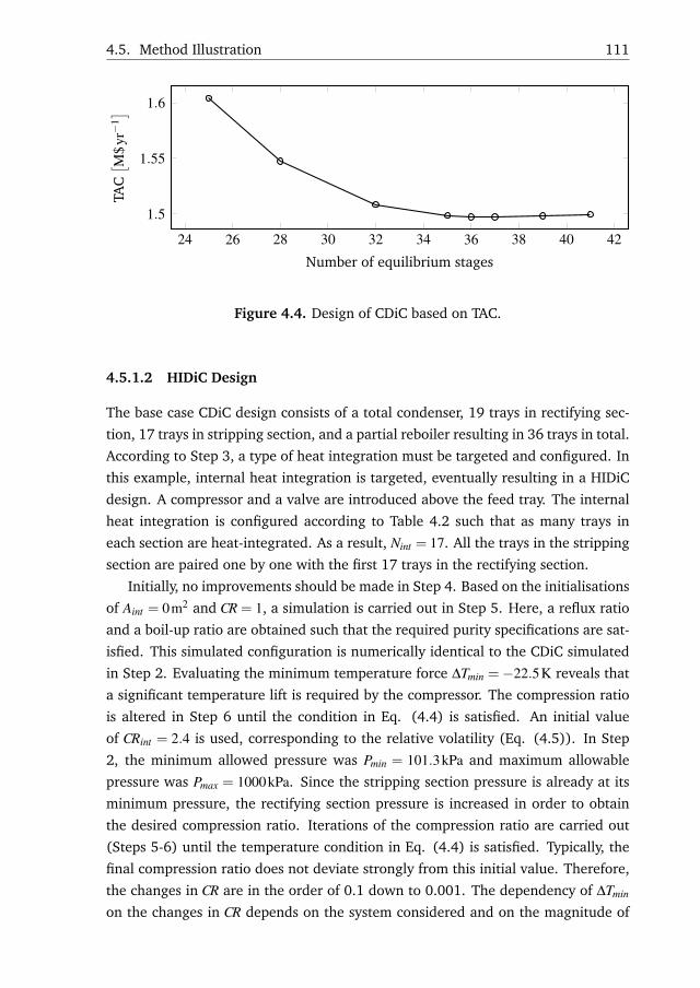
4.5. Method Illustration 111
24 26 28 30 32 34 36 38 40 42
1.5
1.55
1.6
Number of equilibrium stages
TAC[ M
$yr−
1]
Figure 4.4. Design of CDiC based on TAC.
4.5.1.2 HIDiC Design
The base case CDiC design consists of a total condenser, 19 trays in rectifying sec-
tion, 17 trays in stripping section, and a partial reboiler resulting in 36 trays in total.
According to Step 3, a type of heat integration must be targeted and configured. In
this example, internal heat integration is targeted, eventually resulting in a HIDiC
design. A compressor and a valve are introduced above the feed tray. The internal
heat integration is configured according to Table 4.2 such that as many trays in
each section are heat-integrated. As a result, Nint = 17. All the trays in the stripping
section are paired one by one with the first 17 trays in the rectifying section.
Initially, no improvements should be made in Step 4. Based on the initialisations
of Aint = 0m2 and CR = 1, a simulation is carried out in Step 5. Here, a reflux ratio
and a boil-up ratio are obtained such that the required purity specifications are sat-
isfied. This simulated configuration is numerically identical to the CDiC simulated
in Step 2. Evaluating the minimum temperature force ∆Tmin =−22.5K reveals that
a significant temperature lift is required by the compressor. The compression ratio
is altered in Step 6 until the condition in Eq. (4.4) is satisfied. An initial value
of CRint = 2.4 is used, corresponding to the relative volatility (Eq. (4.5)). In Step
2, the minimum allowed pressure was Pmin = 101.3kPa and maximum allowable
pressure was Pmax = 1000kPa. Since the stripping section pressure is already at its
minimum pressure, the rectifying section pressure is increased in order to obtain
the desired compression ratio. Iterations of the compression ratio are carried out
(Steps 5-6) until the temperature condition in Eq. (4.4) is satisfied. Typically, the
final compression ratio does not deviate strongly from this initial value. Therefore,
the changes in CR are in the order of 0.1 down to 0.001. The dependency of ∆Tmin
on the changes in CR depends on the system considered and on the magnitude of

112 Chapter 4. Conceptual Design
A. When A > 0, the pair location of ∆Tmin (pinch) can move during iterations. This
is the case for the separation of benzene/toluene. This observation is believed to
be the reason for the failed attempt in automating this algorithm. For A = 0m2, a
compression ratio of 2.13 results. The key design variables and the resulting TAC
from the mentioned designs are listed in Table 4.5.
The maximum expected heat exchange area can be calculated using Uihx =
0.60kWm−2 K−1 using Eq. (4.1):
Amax =31kJmol−1 ·60.4mols−1
17 ·0.60kWm−2 K−1 ·5K= 36.7m2
The procedure for improving the design by changing the heat exchange area through
Step 4a is as follows: Based on Aint,max the first improvement is A(1) = 0+ 0.30 ·36.7m2 = 11.0m2. Simulation in Step 5 and adjustments in CR are followed in Step
6 until ∆Tmin = 5.0K. A reduction in TAC of 6% is achieved so more iteration should
be followed. In the following iteration A(2) = 11.0m2 + 0.30 · 36.7m2 = 22.0m2 and
a new compression ratio is obtained. These iterations are listed in Table 4.5. An
infeasible design is encountered for A(3) = 33.0m2, the change in A is reduced and
the iterations are repeated. A maximum limit of A was achieved giving A = 30.1m2
and CRint = 2.49. In this design, no reflux is required and thus L/D becomes zero.
Furthermore, TAC=1.76 M$yr−1.
Proceeding, the number of trays (NT ) is incrementally increased by two in each
section. These trays are added in the same vertical height and are heat-integrated
with each other. The total number of stages is increased until a minimum TAC is
obtained similar to the CDiC design. Each time the number of stages is increased,
the pair and the determination of heat exchange area and compression ratio must
be repeated. Only the cases, where A is maximised are shown in Table 4.5 (referred
to as no reflux). These were found to give the lowest TAC.
The design with a minimum TAC (1.72 M$yr−1) has 48 trays in total and 23
pairings. At this point, a design of the HIDiC has been obtained with the simulation
results of the procedure illustrated in Table 4.5. The duties in the final HIDiC design
are Qcnd =−1213kW, Qrbl = 1124kW and E = 402kW, corresponding to a reduction
in the reboiler duty of 65%. Note however, that the TAC is increased compared to
the CDiC.
As can be seen, the TAC is minimum when the heat exchange area is maximised
leading to no external reflux condition (L/D = 0). An important observation is that
when the total number of stages is increased, the HIDiC design becomes infeasible
for unchanged A and CR. This is due to the fact that the total heat exchange area
(NintA) increases since Nint increases.

4.5. Method Illustration 113
Table 4.5. Design Progress of the HIDiC.
A CR Nrct Nstr ∆Tmin OPEX CAPEX TAC Notem2 - - - K M$yr−1 M$ M$yr−1
0 1 19 17 -22.5 1.33 0.840 1.50 Step 20 2.13 19 17 5.0 1.69 2.12 2.12 Step 3-611 2.13 19 17 4.27 1.42 2.79 1.98 Step 4a11 2.188 19 17 5.0 1.41 2.83 1.98 Step 4a-622 2.188 19 17 3.55 1.24 3.24 1.89 Step 4a-622 2.369 19 17 5.0 1.17 3.38 1.84 Step 4a-633 2.369 19 17 3.79 1.03 3.75 1.78 Step 4a-630.1 2.46 19 17 4.7 1.02 3.73 1.77 Step 4a30.1 2.49 19 17 5.0 1.01 3.76 1.76 Step 5-8
(no reflux)24.8 2.48 21 19 5.0 1.00 3.71 1.74 Step 4b-8
(no reflux)21.5 2.47 23 21 5.0 0.98 3.70 1.72 Step 4b-8
(no reflux)19.3 2.46 25 23 5.0 0.97 3.73 1.72 Step 4b-8
(no reflux)17.5 2.45 27 25 5.0 0.96 3.77 1.72 Step 4b-8
(no reflux)
4.5.1.3 MVRC Design
Starting from the CDiC in Step 2, the external heat integration is targeted in Step
3. The same procedure as for the HIDiC is followed, where A and CR now refer to
external heat exchange area and compression ratio. The maximum heat exchange
area is estimated using Eq. (4.2):
Amax =min([3170,3240])kW0.60kWm−2 K−1 ·5K
= 1057m2 (4.10)
The development of the MVRC is illustrated in Table 4.6. Rather than using an
increase in A of 0.3Amax, a value of 0.5Amax is used for illustration as to reduce
the number of rows in Table 4.6. Note that ∆Tmin does not change with the heat
exchange area, thereby simplifying the iteration steps.
In Step 5-6, a valve cooling for the MVRC of Qvlv =−450kW has been obtained.
Without valve cooling, simulation shows that the vapour flow rate is raised from
102 mols−1 to 121 mols−1. Adiabatic throttling is assumed, which leads to a signif-
icant increase in the compressor duty without valve cooling, compared to the case
with valve cooling (from 435 kW to 515 kW). This difference becomes zero using
valve cooling with the provided duty.
Step 4b is investigated by adjusting the total number of trays but the optimal
CDiC appears to result in the optimal MVRC.
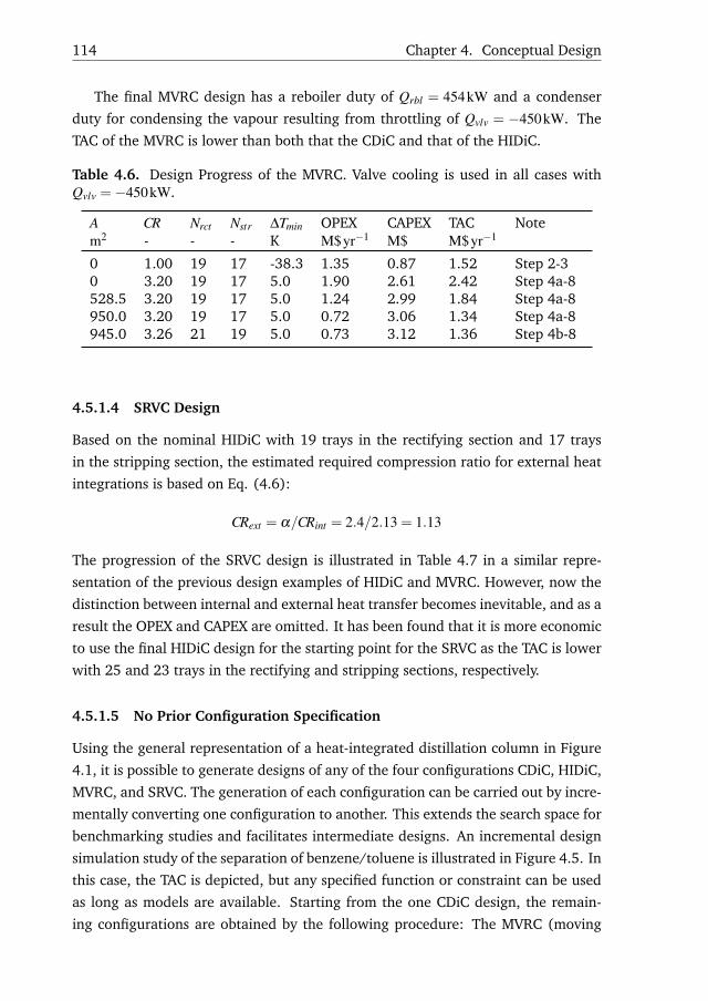
114 Chapter 4. Conceptual Design
The final MVRC design has a reboiler duty of Qrbl = 454kW and a condenser
duty for condensing the vapour resulting from throttling of Qvlv = −450kW. The
TAC of the MVRC is lower than both that the CDiC and that of the HIDiC.
Table 4.6. Design Progress of the MVRC. Valve cooling is used in all cases withQvlv =−450kW.
A CR Nrct Nstr ∆Tmin OPEX CAPEX TAC Notem2 - - - K M$yr−1 M$ M$yr−1
0 1.00 19 17 -38.3 1.35 0.87 1.52 Step 2-30 3.20 19 17 5.0 1.90 2.61 2.42 Step 4a-8528.5 3.20 19 17 5.0 1.24 2.99 1.84 Step 4a-8950.0 3.20 19 17 5.0 0.72 3.06 1.34 Step 4a-8945.0 3.26 21 19 5.0 0.73 3.12 1.36 Step 4b-8
4.5.1.4 SRVC Design
Based on the nominal HIDiC with 19 trays in the rectifying section and 17 trays
in the stripping section, the estimated required compression ratio for external heat
integrations is based on Eq. (4.6):
CRext = α/CRint = 2.4/2.13 = 1.13
The progression of the SRVC design is illustrated in Table 4.7 in a similar repre-
sentation of the previous design examples of HIDiC and MVRC. However, now the
distinction between internal and external heat transfer becomes inevitable, and as a
result the OPEX and CAPEX are omitted. It has been found that it is more economic
to use the final HIDiC design for the starting point for the SRVC as the TAC is lower
with 25 and 23 trays in the rectifying and stripping sections, respectively.
4.5.1.5 No Prior Configuration Specification
Using the general representation of a heat-integrated distillation column in Figure
4.1, it is possible to generate designs of any of the four configurations CDiC, HIDiC,
MVRC, and SRVC. The generation of each configuration can be carried out by incre-
mentally converting one configuration to another. This extends the search space for
benchmarking studies and facilitates intermediate designs. An incremental design
simulation study of the separation of benzene/toluene is illustrated in Figure 4.5. In
this case, the TAC is depicted, but any specified function or constraint can be used
as long as models are available. Starting from the one CDiC design, the remain-
ing configurations are obtained by the following procedure: The MVRC (moving

4.5. Method Illustration 115
Table 4.7. Design Progress of the SRVC.
Aint CRint Aext CRext Nrct Nstr ∆Tmin,int ∆Tmin,ext TAC Notem2 - m2 - - - K K M$yr−1
30.1 2.49 0 1 19 17 5 -3.4 1.76 HIDiCdesign
30.1 2.49 0 1.13 19 17 5 3.8 1.80 CRext es-timate
30.1 2.49 0 1.23 19 17 5 5 1.85 Step 5-830.1 2.49 356 1.23 19 17 5 5 1.45 4a-8
(noreboilerduty)
19.3 2.46 374 1.31 25 23 5 5 1.41 4b-8(noreboilerduty)
left from the CDiC) is obtained by using the maximum possible external heat ex-
change area from Eq. (4.2) such that Tmin = Tcnd −Trbl = 5K. When moving right
from the CDiC in Figure 4.5, internal heat integration is considered and the internal
heat exchange area is gradually increased until no reflux condition is achieved. In
the transition from the HIDiC to the SRVC, external heat integration is considered,
while maintaining Aint and CRint . The external heat transfer area is gradually in-
creased until its maximum. In the SRVC designs to the far right in Figure 4.5, the
internal heat transfer areas are gradually decreased. Note that the conversion of
the HIDiC into an SRVC could similarly be carried out using a smaller internal heat
exchange area. In this example, the influence of changing the total number of trays
has not been investigated.
4.5.2 Multicomponent Aromatic Separation
This example serves as a demonstration of the proposed algorithm on a multicom-
ponent system. Provided the specifications in Table 4.8, the distillate and bottom
product compositions can be estimated when assuming all toluene will leave the
column in the distillate. The conventional distillation column design is provided
by Wakabayashi and Hasebe [160], so the proposed design procedure can be ap-
plied directly. Atmospheric pressure is found to be suitable for the separation. The
CDiC has 30 plates in the rectifying section and 25 plates in the stripping section.
Hence, following the recommendations for pairing for internal heat integration in
Table 4.2, 25 plates in each section should be paired. All the plates in the stripping
116 Chapter 4. Conceptual Design
11.5
22.5
CRin
t[−
]
0200400
Nin
tAin
t[ m
2]
123
CRex
t[−
]
0
500
1,000
Aex
t[ m
2]
MVRC
CDiCHIDiC
HIDiCHIDiC
SRVCSRVC
SRVCSRVC
1.41.61.8
22.2
TAC[ M
$yr−
1]
Figure 4.5. Continuous transition between configurations determined by compres-sion ratios and heat exchange areas. CR denotes the compression ratio while NintAintis the total area of heat exchangers for internal heat integration and Aext is the ex-ternal heat transfer area. The horisontal axes represent distillation column config-urations.
section are paired with the first 25 plates of the rectifying section (counting from
the top) such that they are in the same vertical height, resulting in the HIDiC.
The obtained configurations are summarised in Figure 4.6, in which the capital
expenditures (CAPEX) is illustrated along with the operating expenditures (OPEX).
The obtained results are compared to the novel HIDiC configuration called the 4-
HIDiC, which is based on the Extended Ponchon-Savarit method [159] and has
only four internally heat-integrated pairs. The 4-HIDiC outperforms the HIDiC as

4.5. Method Illustration 117
Table 4.8. Feed specification of the separation of a multicomponent aromatic mix-ture.
Specification Property Unit Value
Feed flow rate kmol s-1 55.6Feed composition Toluene (C7) - 0.005
Ethylbenzene (C8) - 0.1p-Xylene (C8) - 0.11m-Xylene (C8) - 0.25o-Xylene (C8) - 0.145Cumene (C9) - 0.01n-Propylbenzene (C9) - 0.022m-Ethyltoluene (C9) - 0.1581,2,3-Trymethylbenzene(C9)
- 0.2
Liquid fraction - 1Feed pressure kPa 101.3Feed temperature K 421.3Stage pressure drop kPa 0.70Top purity specifica-tion
C9 - 0.007
Bottom purity speci-fication
C8 - 0.015
a result of decreased CAPEX by using fewer, but larger, heat exchangers and lower
duty of the compressor. At the same time the MVRC outperforms the HIDiC as well
as the 4-HIDiC . The lowest OPEX but the highest CAPEX is obtained in the SRVC.
Thus, in order to fully benefit from heat integration among stages one would prefer
the SRVC, or alternatively stay with the MVRC. This suggests that tools for design
decisions must be broadly applicable and be able to consider various alternatives
in order to be versatile. It is not enough to merely compare HIDiC to CDIC. A
framework, which is flexible and on a general form, is useful for such studies.
1 2 3 4 5
1
1.5
CDiC
MVRC
HIDiC
SRVC
4-HIDiC
CAPEX [M$]
OPE
X[ M
$yr−
1]
Figure 4.6. Illustration of the trade-off between OPEX and CAPEX for five configu-rations performing a separation of a multicomponent aromatic mixture.

118 Chapter 4. Conceptual Design
4.6 Design Considerations and Discussion
A discussion of the design method is presented in this section. The discussion is
based on qualitative considerations, simple models and the case study of benzene/-
toluene, provided in section 4.5.1. The base case HIDiC design, resulting directly
from the CDiC design, is employed.
4.6.1 Stripping Section Pressure
The selection of stripping section pressure, which is referred to as the feed stage
pressure (PNF), has been given little attention in the HIDiC design literature. The
optimal design value of PNFis assumed to be a trade-off between operating and
capital costs. The contributions to the operating costs are the addition of external
utility (condenser and reboiler duties) and the cost of electricity for compression.
A low pressure is favoured in terms of minimising the quality of the heat supplied
as reboiler duty (e.g. reduced steam pressure). However, the compressor duty is
a dominant factor in both OPEX and CAPEX in many cases. For example in the
separation of benzene/toluene, the compressor accounts for 53% OPEX and 45%
CAPEX. The compressor duty in Eq. (2.2) can be written for an as:
E =1
ηisVinTinCV
P
(CRR/CV
P −1)
(4.11)
where
Vin = vapour flow through compressor [mole/s]Tin = temperature at compressor inlet [K]
CVP = constant pressure heat capacity of vapour [kJmol−1 K−1].
As it appears in Eq. (4.11), the compressor duty is proportional to the inlet tem-
perature, which is determined by the operating pressure (PNF). Furthermore, the
compressor duty increases with the compression ratio to the power of R/CVP . This
exponent is relatively small for larger molecules (e.g. monoatomic gas R/CVP = 2/3,
diatomic R/CVP = 2/5 etc.). Hence, based on the inlet temperature, a low operating
pressure is preferred in order to minimise the compressor duty. When the mini-
mum temperature driving force (∆Tspec) is infinitesimally small, the compression
ratio can be approximated by the relative volatility for the MVRC (Eq. (4.5)). The
temperature dependency of the relative volatility is typically small. Therefore, the
influence of the operating pressure on the relative volatility, and hence the com-
pression ratio in Eq. (4.11), can be neglected. It can be concluded, that the impact
of the operating pressure on the inlet temperature (Tin) is more significant than the
impact on the compression ratio.

4.6. Design Considerations and Discussion 119
It is found that indeed the compressor duty increases with the feed stage pres-
sure, when investigating its impacts on the compressor duty, the CAPEX, and the
OPEX by carrying out simulations for benzene/toluene (see Table 4.9). In addition,
it is found in agreement with the analysis that the CAPEX increases with feed stage
pressure as well. However, the opposite effect is observed for the OPEX. This is due
to the fact that the required compression ratio increases as the fixed stage pressure
drop becomes more significant when the operating pressure is lowered. As a result
of this analysis, a low operating pressure in the low pressure section is desired. For
this reason, it is proposed to reduce the pressure of the low pressure side of a com-
pressor as first priority in step 6 (Figure 4.2). Furthermore, these results illustrate
the importance of considering stage pressure drops when evaluating the economic
performance of a heat-integrated configuration.
Table 4.9. Sensitivity on compressor duty, CAPEX and OPEX of column operatingpressure when applying the design method on the separation of benzene/toluene.
PNFCRint Tin E CAPEX OPEX
kPa - K kW M$ M$yr−1
75 2.59 357 388 3.87 1.03101 2.45 367 394 3.92 1.02125 2.37 374 401 4.00 1.02
4.6.2 Interplay Between Design Variables
When thermodynamic feasibility is realised (i.e. the minimum temperature driving
force is positive), the expression for the internal heat transfer rate (Eq. (3.29))
states that an increase in ∆T by 1 unit corresponds to an increase in A by 1 unit.
Increases in both OPEX and CAPEX result when ∆T is increased by compression.
However, the increase in ∆T happens for all the pairs simultaneously. On the con-
trary, A must be increased for all pairings, which might result in a significant in-
crease in CAPEX for a large number of heat-integrated stages. Thus, a trade-off
between CAPEX and OPEX is not only reflected in choosing number of stages vs. re-
flux ratio as in CDiC but also generating a temperature driving force by increasing
CR without increasing it excessively.
The relation between compression ratio and heat exchanger areas is investigated
by carrying out HIDiC designs for obtaining reflux free operation of the separation
of benzene/toluene. The result is illustrated in Figure 4.7. As expected, (Eq. (4.5)),
compression ratios below the relative volatility have significant impact on the re-
quired total heat exchange area, since certain pairings have low heat transfer rates
due to small temperature gradients. On the other hand, when the heat exchange

120 Chapter 4. Conceptual Design
area is small, the compressor must compensate and provide large temperature gra-
dients and thus a large compression ratio is required.
The optimal solution has both a low CR and a low A in figure 4.7. Hence, it is
reasonable to base a the design on the minimum temperature driving force. If this
is set reasonably low, the optimal trade-off of CR and A is expected to be achieved.
Based on this analysis, it has been found useful to use the heat exchange area and
the temperature driving force as design variables.
5 10 15 20 25 30 35 40 45 50
2
2.5
3
3.5
4
4.5
∆Tmin = 5K
α12 = 2.34
Aint[m2]
CRin
t[−
]
Figure 4.7. Relation between compression ratio and heat exchange area for theseparation of benzene/toluene.
4.6.3 Constant Area Versus Constant Heat Duty
As indicated in Figure 4.1, the heat exchange area must be specified for each in-
ternal heat exchanger corresponding to every pair. Since the temperature driving
forces vary along the column, constant heat transfer duties can lead to an uneven
distribution of heat transfer area as illustrated in Figure 4.8. An alternative strategy
is to design a constant heat transfer area for all stages. The total required heat

4.6. Design Considerations and Discussion 121
exchange areas are obtained is section 4.5.1 as 438 m2 and 427 m2 for respectively
the constant heat transfer area (Aint,n = 30.1m2, n = 1,2, . . . ,Nint) and for the con-
stant internal heat transfer rates (qn = 89.6kW, n = 1,2, . . . ,Nint with Aint,n from Eq.
(3.29)). The contribution of the internal heat exchangers for the constant heat ex-
change area approach on the CAPEX is 1.41 M$, while for the constant heat duty
it is 1.35 M$. However, when considering the compressor duty, the constant heat
duty design has a 7% higher compressor duty (from 394 to 421 kW) leading to a
higher OPEX. The comparison between these strategies shows that (i) the total heat
exchange area (3%) and the CAPEX (5%) is slightly larger for the constant heat
exchange area approach, (ii) a strong coupling exists between the required heat
exchange areas and the column temperature profile for the case of constant heat
duties, (iii) from a practical view, however, it is simpler and most likely cheaper
when only small variations in the heat exchange areas occur, and (iv) it appears
more economically favoured to adopt a constant heat exchange area approach in
terms of OPEX. It has been confirmed by others [154] that the constant heat ex-
change area approach for the separation of benzene/toluene results in the best
economic performance.
1 2 3
0
0.5
1
Column area[m2]R
elat
ive
colu
mn
heig
ht[-
]
10 20 300
10
20
Aint,n[m2]
Pair
num
ber,
n[-
]
Figure 4.8. Estimated column area and the required heat exchange area for noreflux operation for two cases: Constant heat exchange area vs. constant heat dutyfor each pair. Legends: Constant Aint ( ), Constant qint ( ).
4.6.4 Method Benchmarking
A summary of the resulting HIDiC designs, based on different methods for a sepa-
ration of methanol/water into 90% top and 10% bottom purities, is given in Table
4.10. The methods have different purposes, which is reflected in the results. A
remarkable difference among the illustrated design results are the obtained com-

122 Chapter 4. Conceptual Design
pressor duties (E). The reason for this is that the considered methods do not adopt
the minimum temperature approach. This approach can not be used in graphi-
cal methods due to the strong coupling with the mass and energy balances of the
complete design. If the model framework developed in this work is available, it is
claimed that proposed method can be conducted with less efforts than the consid-
ered graphical methods.
Table 4.10. Comparison of HIDiC designs using proposed method and literaturemethods.
Method Design variablesNrct Nstr E Qrbl ∑qn Nihx An
- - kW kW kW - m2
Proposed method 6 5 109.3 1428 662 4 26.7, 26.7,26.7, 26.7
Ponchon-Savaritmethod [56]
5 4 261.2 1317 600 4 18.2, 10.8,9.0, 8.4
Extended Ponchon-Savarit method[159]
3 6 250 1232 888 3 18.3, 19.5,14.4
4.7 Conclusion
A design method that can cover the three heat-integrated distillation configura-
tions is proposed; the mechanical-vapour recompression column (MVRC), the heat-
integrated distillation column (HIDiC), and the secondary reflux and vaporisation
column (SRVC). Following advantages of the design algorithm are claimed:
• It provides a systematic means of selecting the additional design variables of
the MVRC, the HIDiC, and the SRVC
• It provides a systematic means of evaluating the most economically preferred
configuration among the MVRC, the HIDiC, and the SRVC
• It is simple and intuitive
• It can explicitly cover multicomponent mixtures
However, on present form, an fully optimal design is not guaranteed.
In this chapter, the presented method has been successfully applied on the sep-
aration of two binary separations (benzene/toluene and methanol/water) and a
multicomponent separation.

Chapter5
Techno-Economic Feasibility Analysis
Techno-economic feasibility analyses are carried out for the
heat-integrated distillation columns (HIDiC) separating ben-
zene/toluene and propylene/propane. The techno-economic
feasibility analysis address the physical realisation of heat trans-
fer equipment, the possibility of entrainment flooding and
weeping in different column arrangements, and benchmark-
ing of alternative distillation configurations w.r.t. economy. A
simple relation for evaluating the requirement for compressor
vapour inlet super-heating is derived. Furthermore, an exten-
sive economic feasibility analysis is presented covering ten in-
dustrial mixtures with different physical properties, to be sep-
arated in the conventional distillation column, the HIDiC, the
mechanical vapour recompression column (MVRC), and the sec-
ondary reflux and vaporisation column (SRVC). It was found
that the normal boiling point difference was correlated with the
major design variables and performance indicators. In terms
of the total annualised cost (TAC), the MVRC is the preferred
configuration for the majority of the considered configurations.
However, the HIDiC is the preferred configuration with respect
to operating expenditures (OPEX) when the normal boiling
point difference is below 10 K. The uncertainties in the OPEX
for an MVRC and an HIDiC were quantified by the means of un-
certainty analysis, and the most significant parameters on the
OPEX uncertainty were identified for the two configurations.

124 Chapter 5. Techno-Economic Feasibility Analysis
The uncertainty and sensitivity analysis results were presented
at the Distillation and Absorption conference [T. Bisgaard, J.K.
Huusom, and J. Abildskov. Impact on model uncertainty of dia-
batization in distillation columns. Proceedings of Distillation andAbsorption, pages 909–914, 2014].
5.1. Introduction 125
5.1 Introduction
The conventional distillation column (CDiC), the mechanical vapour recompres-
sion column (MVRC), the heat-integrated distillation column (HIDiC), and the sec-
ondary reflux and vaporisation column (SRVC) are studied in this chapter. The
economic feasibilities of the considered configurations are often linked to either the
relative volatility [51, 48], the normal boiling point difference [86], or the resulting
temperature profiles of the columns [142]. It is the aim of this chapter, to identify
the links between the mixture properties, the design variables, and the economic
feasibilities for the considered configurations. If such links exist, it is desired to use
the physical properties of the mixtures to be separated as a means of determining
the economically preferred distillation column configuration. Such an approach is
similar to the framework proposed by Jaksland et al. [72] for conventional unit
operations. The present analysis has been restricted to cover mainly binary mix-
tures; one multicomponent mixture is covered. However, the mixtures are carefully
selected in order to cover a variety of the following physical properties:
• Difference in normal boiling points.
• Mean heat of vaporisation.
• Phase equilibrium behaviour (ideal, non-ideal, azeotropic etc.)
The phase equilibrium behaviour is used as a means to cover different resulting col-
umn temperature profiles rather than adjusting the product purities. Furthermore,
the economic feasibility of a configuration is based on both the total annualised cost
(TAC) and the operating expenditures (OPEX).
5.2 Methods and Tools
The considered case studies and the methods, used throughout this chapter, are
briefly explained in this section. The terms technical feasibility and economic feasi-
bility are defined.
5.2.1 Technical Feasibility
The following criteria must be satisfied in order to achieve technical feasibility of a
given heat-integrated distillation configuration:
• Feasible solution: The first criteria for technical feasibility requires that a fea-
sible solution to the distillation column model exists, given the feed and the
product specifications.

126 Chapter 5. Techno-Economic Feasibility Analysis
• Realisation of internal heat transfer: The distillation column internals must
have sufficient space for the installation of internal heat panels. The hy-
draulic feasibility indicator (HFI; Section 3.4) is suitable for this purpose.
When HFI>1, the column can accommodate the specified heat exchange area
by installing heat panels in the stripping section.
• Column capacity: Based on an estimated column cross sectional area, the
possibility of using conventional sieve trays is investigated. Hence, no en-
trainment flooding or weeping must occur. In addition, the various column
profiles of flows, heat transfer rates, temperatures and so on, provides valu-
able insights in the technical feasibility.
• Feasibility of compression: Condensation must not occur inside a compres-
sor. Hence, the possibility of condensation of the compressed vapour must
be investigated, and appropriate actions must be taken if it is the case. One
action that can prevent condensation in the compressor is to superheat the
compressor inlet vapour.
The above criteria are explained in detail in the following subsections.
5.2.1.1 Column Capacity
Based on conventional methods for investigating column tray capacities [57], the
impact of introducing internal heat transfer is investigated w.r.t. entrainment flood-
ing or weeping. Below the weeping point, at which the vapour flow rate is too
low compared to the design flow rate, the required vapour dispersion can not be
achieved. Furthermore, the vapour flow is not sufficient to prevent the liquid from
passing through the perforations. The latter can be avoided by using bubble cap
or valve trays. Entrainment flooding occurs when the vapour flow rate is too high.
With increasing vapour flow rate, an increasing amount of liquid is entrained until a
point where flooding occurs. As a result, the downcomers are filled and the column
feed will be carried up through the column with the vapour. A large increase of
pressure drop across the column is observed. Mathematically, flooding is avoided
when 0 ≤ ucrit,i− ui, i.e. when the vapour velocity is below the flooding velocity
(ucrit). Weeping is avoided when 0≤ (Hσ +H0)− (Hσ +H0)crit , corresponding to the
fact that the liquid head must not exceed the pressure drop from vapour passing
through the perforations (H0) and through the liquid due to surface tension (Hσ ).
The critical pressure drop (Hσ +H0)crit depends on the liquid head, which is the
sum of hoW +hW [57].
The column sizing methods are usually based on the idea of avoiding flooding
at nominal operation, but due to constructional implications of introducing inter-

5.2. Methods and Tools 127
nal heat transfer this might influence the tray capacities. One constructional im-
plication is the gradually decreasing stripping section cross sectional area and the
gradually increasing rectifying section cross sectional area from the column top to
the bottom. As a result, the impacts of different design decisions (e.g. constant tray
area vs. gradually changing tray area) on the technical feasibility are investigated.
Three concentric arrangements are considered (Table 2.3):
• An arrangement, where the cross sectional area is constant throughout the
column.
• A concentric arrangement with gradually changing cross sectional areas of the
rectifying and stripping sections. The rectifying section constitutes the inner
(tube) column and the stripping section constitutes the outer (shell) column.
• A 3-partition concentric arrangement, which is divided in three different par-
titions of equal height. The cross sectional areas of the inner rectifying section
are different in each partition as a means to simplify the concentric arrange-
ment. In this work, the cross sectional area of a partition is given by the mean
value of the obtained cross sectional areas of the trays within the partition.
Table 5.1. Sieve tray dimensional parameters provided total cross sectional area.
Parameter Unit Value
Hole diameter mm 6.35Weir height mm 50Downcomer area per total area - 0.1Perforations area per active tray area - 0.1Tray thickness per hole diameter - 0.72
5.2.1.2 Feasibility of Compression
The feasibility of compression (FOC) is defined by:
FOC =ηisλ
CVP Tnb
−1 (5.1)
The FOB is derived by evaluating the change in the saturated temperature rela-
tive to the temperature change caused by isentropic compression. Condensation,
due to compression, is undesired. Thus, the temperature increase, caused by com-
pression, should be larger than the increase in the dew point temperature. This
translates into a condition that states that FOC should be greater than zero. If the
FOC is below zero, condensation might occur. This issue is not widely considered
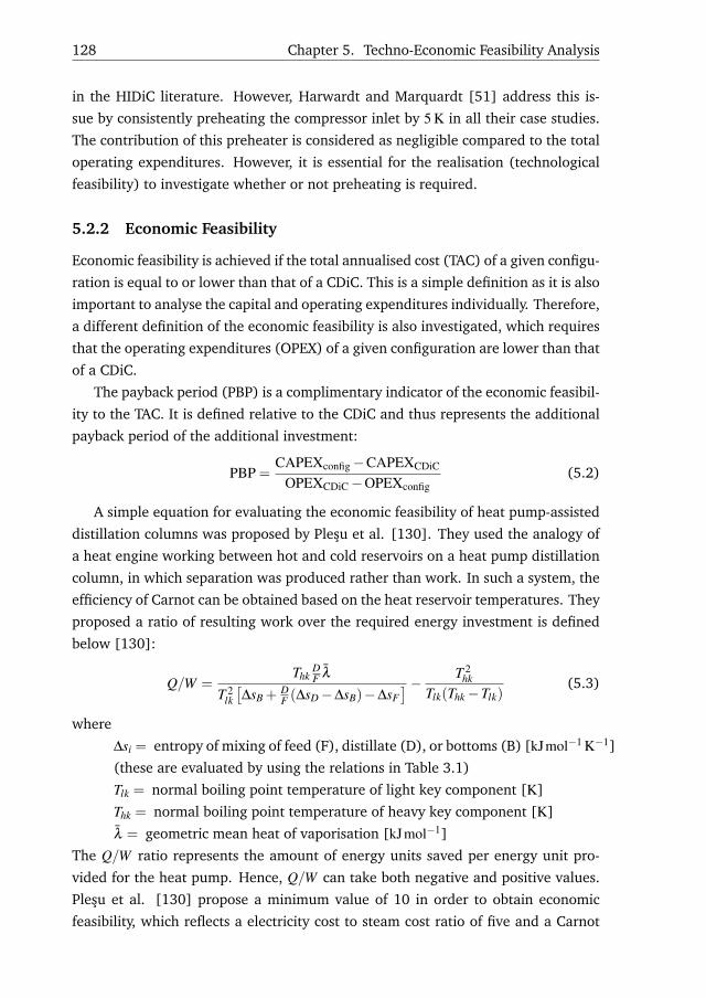
128 Chapter 5. Techno-Economic Feasibility Analysis
in the HIDiC literature. However, Harwardt and Marquardt [51] address this is-
sue by consistently preheating the compressor inlet by 5 K in all their case studies.
The contribution of this preheater is considered as negligible compared to the total
operating expenditures. However, it is essential for the realisation (technological
feasibility) to investigate whether or not preheating is required.
5.2.2 Economic Feasibility
Economic feasibility is achieved if the total annualised cost (TAC) of a given configu-
ration is equal to or lower than that of a CDiC. This is a simple definition as it is also
important to analyse the capital and operating expenditures individually. Therefore,
a different definition of the economic feasibility is also investigated, which requires
that the operating expenditures (OPEX) of a given configuration are lower than that
of a CDiC.
The payback period (PBP) is a complimentary indicator of the economic feasibil-
ity to the TAC. It is defined relative to the CDiC and thus represents the additional
payback period of the additional investment:
PBP =CAPEXconfig−CAPEXCDiC
OPEXCDiC−OPEXconfig(5.2)
A simple equation for evaluating the economic feasibility of heat pump-assisted
distillation columns was proposed by Plesu et al. [130]. They used the analogy of
a heat engine working between hot and cold reservoirs on a heat pump distillation
column, in which separation was produced rather than work. In such a system, the
efficiency of Carnot can be obtained based on the heat reservoir temperatures. They
proposed a ratio of resulting work over the required energy investment is defined
below [130]:
Q/W =Thk
DF λ
T 2lk
[∆sB +
DF (∆sD−∆sB)−∆sF
] − T 2hk
Tlk(Thk−Tlk)(5.3)
where
∆si = entropy of mixing of feed (F), distillate (D), or bottoms (B) [kJmol−1 K−1]
(these are evaluated by using the relations in Table 3.1)
Tlk = normal boiling point temperature of light key component [K]
Thk = normal boiling point temperature of heavy key component [K]
λ = geometric mean heat of vaporisation [kJmol−1]
The Q/W ratio represents the amount of energy units saved per energy unit pro-
vided for the heat pump. Hence, Q/W can take both negative and positive values.
Plesu et al. [130] propose a minimum value of 10 in order to obtain economic
feasibility, which reflects a electricity cost to steam cost ratio of five and a Carnot

5.2. Methods and Tools 129
efficiency of two. Note that the geometric mean heat of vaporisation has been
used rather than the distillate heat of vaporisation. It is assumed that this exten-
sion can describe the HIDiC as well as the heat pump-assisted distillation column,
for which the expression was originally developed [130]. For a binary separation
D/F = (xD− z)/(xD− xB).
5.2.3 Uncertainty and Sensitivity Analysis
An uncertainty analysis is carried out in order to quantify the uncertainty in the op-
erating expenditures (OPEX) of a given configuration when the model parameters
and the economic parameters are uncertain. Furthermore, a sensitivity analysis
is employed in order to identify the parameters that cause the uncertainty in the
OPEX. These are essential considerations when the economic feasibility of config-
urations is evaluated. The underlying theories for the uncertainty and sensitivity
analysis are briefly stated in this section.
5.2.3.1 Monte Carlo Simulation
Any model can be represented in the general form:
x = f(x,u,θθθ) (5.4)
0 = h(x,u,θθθ) (5.5)
y = g(x,u,θθθ) (5.6)
where
x = the state derivative of length Nx
x = the state variable vector of length Nx
u = the input vector with length Nu
θθθ = the model parameter vector with length Nθθθ
y = output vector with length Ny
The model parameter vector can be divided in two θθθ = [θθθ ∗,θθθ ∗]T , where θθθ ∗ rep-
resents the uncertain parameters of the parameter vector, while θθθ∗ represents the
certain parameters.
Let i = 1,2, . . . ,Ny denote the index of the model output, let j = 1,2, . . . ,Nθθθ∗
denote the index of the uncertain parameter, and let p = 1,2, . . . ,Np denote the
Monte Carlo discretisation point. Hence, the model uncertainty can be evaluated
by the Monte Carlo Method [102], in which the expectation and variance of the
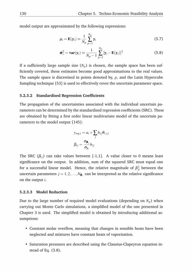
130 Chapter 5. Techno-Economic Feasibility Analysis
model output are approximated by the following expressions:
µi = E(yi)≈1
Np
Np
∑p=1
yi (5.7)
σσσ2i = var(yi)≈
1Np−1
Np
∑p=1
[yi−E(yi)]2 (5.8)
If a sufficiently large sample size (Np) is chosen, the sample space has been suf-
ficiently covered, these estimates become good approximations to the real values.
The sample space is discretised in points denoted by, p, and the Latin Hypercube
Sampling technique [53] is used to effectively cover the uncertain parameter space.
5.2.3.2 Standardised Regression Coefficients
The propagation of the uncertainties associated with the individual uncertain pa-
rameters can be determined by the standardised regression coefficients (SRC). These
are obtained by fitting a first order linear multivariate model of the uncertain pa-
rameters to the model output [145]:
yreg,i = ai +∑j
bi jθ∗,i j
βi j =σθθθ j
σyi
bi j
The SRC (βi j) can take values between [-1,1]. A value closer to 0 means least
significance on the output. In addition, sum of the squared SRC must equal one
for a successful linear model. Hence, the relative magnitude of β 2ji between the
uncertain parameters j = 1,2, . . . ,Nθθθ∗ can be interpreted as the relative significance
on the output i.
5.2.3.3 Model Reduction
Due to the large number of required model evaluations (depending on Np) when
carrying out Monte Carlo simulations, a simplified model of the one presented in
Chapter 3 is used. The simplified model is obtained by introducing additional as-
sumptions:
• Constant molar overflow, meaning that changes in sensible heats have been
neglected and mixtures have constant heats of vaporisation.
• Saturation pressures are described using the Clausius-Clapeyron equation in-
stead of Eq. (3.8).

5.3. Feasibility Indicators – Observations and Expectations 131
• Physical properties are no longer dependant on temperature, pressure and
composition. This also implies a constant relative volatility.
• Ideal, binary mixtures.
The model variables are classified according to Eqs. (5.4)-(5.6):
x = (x1, ...,xNS)T (5.9)
u = (PF ,CR,Lcnd ,Vrbl ,F,z)T (5.10)
θθθ = (λ ,Tnb,1,∆Tnb,∆P,Uihx,A,CVP ,Swater,Ssteam,Selectricity,Nrct ,Nstr)
T (5.11)
y = (OPEX) (5.12)
where
Tnb,1 = normal boiling point temperature of light component [K]
∆Tnb = normal boiling point temperature difference of components [K]
∆P = Tray pressure drop [kPa]
The obtained model is similar to the one proposed by Huang et al. [60] if pres-
sure drops were included, if the Antoine correlation was replaced by the Clausius-
Clapeyron equation, and if column sections of different sizes were allowed.
5.3 Feasibility Indicators – Observations and Expectations
The selection of industrial binary separations are listed in Table 5.2. Both the Q/W
ratio in Eq. (5.3) and the feasibility of compression in Eq. (5.1) are estimated and
listed in the table. Some clear trends are observed: (i) The high Q/W ratios are
observed for the mixtures with low relative volatilities meaning potential economic
feasibilities, (ii) the FOC is negative for the mixtures comprised of large molecules
as the heat capacities are high, which means that condensation due to compression
might be a risk, and (iii) no significant relation between heats of vaporisation, Q/W
and FOC are present. According to the Q/W estimates, mixtures with a relative
volatility below 1.83 are expected to be economically feasible.

132 Chapter 5. Techno-Economic Feasibility Analysis
Tabl
e5.
2.Fe
asib
ility
indi
cato
rsof
indu
stri
ally
rele
vant
,bi
nary
mix
ture
s.Th
elis
tof
mix
ture
san
dth
eir
rela
tive
vola
tilit
ies
are
obta
ined
from
Sead
eret
al.
[137
].Th
em
ixtu
res
are
sort
edac
cord
ing
toin
crea
sing
rela
tive
vola
tilit
y.Th
eph
ysic
alpr
oper
ties
are
take
nfr
omN
IST
[120
].Th
ees
tim
atio
nof
Q/W
isba
sed
onfo
llow
ing
sepa
rati
on:
x D=
1−
x B=
0.99
5an
dz=
0.5,
whi
leη
is=
0.80
inth
eFO
C.T
hem
ean
phys
ical
prop
erti
esar
ere
pres
ente
dby
geom
etri
cm
ean
valu
es.
Mix
ture
com
pone
nts
α∆T
nbT n
bλ
CV P
Q/W
FOC
Ligh
t/H
eavy
-K
KkJ
mol−
1kJ
mol−
1K−
1-
-
1,3-
But
adie
ne/v
inyl
acet
ylen
e1.
167.
527
2.3
23.6
0.00
764
28-0
.1Vi
nyla
ceta
te/e
thyl
acet
ate
1.16
4.5
347.
936
.10.
1061
66-0
.2m
-Xyl
ene/
o-xy
lene
1.17
4.7
414.
641
.50.
1291
78-0
.4Is
open
tane
/n-p
enta
ne1.
308.
130
5.1
25.6
0.11
9529
-0.4
Isob
utan
e/n-
buta
ne1.
3511
.026
7.4
21.2
0.09
757
16-0
.4Et
hylb
enze
ne/s
tyre
ne1.
389.
741
4.1
42.4
0.12
3733
-0.3
Prop
ylen
e/pr
opan
e1.
405.
522
8.3
16.1
0.06
880
34-0
.2M
etha
nol/
etha
nol
1.44
13.7
344.
640
.20.
0536
014
0.7
Wat
er/a
ceti
cac
id1.
8318
.038
2.1
45.4
0.04
876
111.
0Et
hyle
ne/e
than
e1.
8715
.617
6.6
14.6
0.47
454
0.4
Ace
tic
acid
/ace
tic
anhy
drid
e2.
0220
.840
1.5
46.7
0.07
945
70.
2To
luen
e/et
hylb
enze
ne2.
1525
.539
6.3
38.9
0.11
496
-0.3
Prop
ane/
1,3-
buta
dien
e2.
1837
.524
9.1
18.7
0.07
664
1-0
.2Et
hano
laze
otro
pe/w
ater
2.21
21.7
362.
241
.40.
0494
35
0.9
Isop
ropa
nol/
wat
er2.
2317
.736
4.2
42.4
0.05
785
90.
6B
enze
ne/t
olue
ne3.
0930
.536
8.2
35.4
0.09
246
3-0
.2M
etha
nol/
wat
er3.
2735
.435
5.0
38.8
0.04
063
01.
2C
umen
e/ph
enol
3.76
30.0
439.
750
.90.
1242
5-0
.3B
enze
ne/e
thyl
benz
ene
6.79
56.0
380.
337
.30.
1025
-1-0
.2H
ydro
genc
yani
de/w
ater
11.2
74.2
334.
031
.80.
0515
8-2
0.5
Ethy
lene
oxid
e/w
ater
12.6
888
.232
6.1
32.2
0.04
197
-20.
9Fo
rmal
dehy
de/m
etha
nol
16.7
83.8
292.
930
.20.
0394
9-3
1.1
Wat
er/e
thyl
ene
glyc
ol81
.297
.341
9.0
51.0
0.05
406
-30.
8

5.4. Case Studies 133
5.4 Case Studies
Two case studies representing two classes of mixtures are presented: A wide-boiling
mixture of benzene/toluene and a close-boiling mixture of propylene/propane.
5.4.1 Benzene/toluene
The separation of benzene/toluene is commonly considered a representative sepa-
ration for illustrating the concepts of e.g. the HIDiC. The boiling point difference
between the two components is 30.5 K as listed in Table 5.2. Therefore, the mix-
ture is considered as a wide-boiling mixture. This mixture has a large difference
in normal boiling points, which is reflected in the low Q/W = 3. According to the
preliminary feasibility analysis, the separation of benzene/toluene is not expected
to be economically feasible.
5.4.1.1 Conceptual Design
The designs of the four configurations (CDiC, MVRC, HIDiC, and SRVC) are already
provided in Section 4.5.1. This section presents a detailed analysis of the technolog-
ical and economic aspects of the internal heat integration. Therefore, this section
mainly concerns the HIDiC, but a complete benchmark study is carried out for all
the four configurations.
5.4.1.2 Technical Feasibility
The tray mole fractions, tray temperatures, and internal flow rates are shown in
Figure 5.1 of an HIDiC along with the ones of a CDiC. As expected, the liquid and
vapour flow rates are almost constant for the CDiC throughout the column, except
at the feed location. In the HIDiC, the liquid and vapour flows gradually increases
until a maximum is reached in the transition between the column sections. The
mole fraction profile is significantly different in the HIDiC than in the CDiC. The
shape of the CDiC mole fraction profile is caused by a pinch point as the operat-
ing point is close to the minimum reflux condition. The HIDiC has a more even
composition profile due to internal heat integration [43]. The difference in the
composition profiles are reflected in the temperature profiles. Furthermore, a tem-
perature lift of 29 K, provided by the compressor, is illustrated in the temperature
profile.
The estimated total tray cross sectional areas for each tray in a CDiC is approxi-
mately constant (Figure 5.2). In contrast, the variations of the internal flows in the
HIDiC (Figure 5.1) causes significant variation in the total tray cross sectional area

134 Chapter 5. Techno-Economic Feasibility Analysis
0 50 100 150
0
0.5
1
Flow rate[mols−1
]
Rel
ativ
eco
lum
nhe
ight
0 0.5 1
0
0.5
1
Mole fraction [−]360 380 400
0
0.5
1
Temperature [K]
Figure 5.1. Tray internal flow rates, benzene mole fractions, and tempearturesof the HIDiC and the CDiC separating benzene/toluene. Legend: HIDiC: Molefraction and temperature ( ), liquid flow rate ( ), vapour flow rate ( ),temperature outlet of compressor ( ). CDiC: Mole fraction and temperature ( ),liquid flow rate ( ), vapour flow rate ( ).
profile in Figure 5.2. When combining the total tray cross sectional area of the trays
that are heat-integrated, an approximately uniform combined total tray cross sec-
tional area is achieved. This observation favours the concentric arrangement. The
HFI is calculated and plotted in Figure 5.3. Based on the HFI profile, it can be con-
cluded that the specified heat exchange areas (19.3 m2 for each pair) can be realised
as HFI>1 for almost every pair. In addition, the temperature driving forces seem
reasonable compared to typical specifications in conventional heat exchangers.
0.5 1 1.5 2 2.5 3 3.5
0
0.5
1
Areas[m2]
Rel
ativ
eco
lum
nhe
ight
HIDiCCDiC
Figure 5.2. Required total tray areas for a HIDiC and a CDiC for the separation ofbenzene/toluene.

5.4. Case Studies 135
5 10 15
0
10
20
Pinch, n = 15
Temperature driving force [K]
Hea
tin
tegr
ated
pair,
n
1 1.5 2 2.5
0
10
20
HFI [−]
Figure 5.3. The temperature driving forces among heat-integrated pairs and thecorresponding hydraulic feasibility indicator (HFI) for the separation of benzene/-toluene. Physical realisation of the specified heat exchange area (Aint = 19.3m2) ispossible for HFI>1.
Ideally the column area profiles would follow that of Figure 5.2 for both the
CDiC and the HIDiC. A column with a uniform cross sectional area is commonly
used for the CDiC. An investigation of the possibility of simplifying the HIDiC struc-
ture is conducted. Figure 5.4 illustrates the implications of the three different ar-
rangements (concentric, 3-partition concentric, uniform area) on the column capac-
ity w.r.t. entrainment flooding and weeping. The results show that the concentric
and the 3-partition concentric column arrangements are feasible. The uniform area
column is not feasible because weeping is predicted in the top of the column. Weep-
ing can be avoided by using other tray specifications or by using valve or bubble-
cap trays. However, valve or bubble-cap trays take up more space inside a tray, and
therefore reduce the available space for the required heat panels.
The feasibility of compression was reported for benzene/toluene in Table 5.2.
Based on geometric mean pure component parameters the value is FOB=-0.2. By
retrieving the properties of the inlet vapour stream from the simulation results and
using these in Eq. (5.1), the FOB becomes:
FOB =0.80 ·29.62kJmol−1
0.1218kJmol−1 K−1366.7K−1 =−0.4695
Hence, the same conclusion is resulted as the calculation based on the pure compo-
nent properties. Because FOB is negative, it is expected that increasing the pressure
of the saturated vapour, by means of isentropic compression, will result in a sub-
cooled vapour. The obtained compressor outlet temperature from simulation agrees
with the result; the temperature of the vapour outlet of the compressor is 396 K as
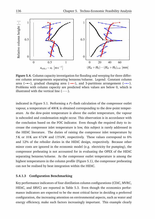
136 Chapter 5. Techno-Economic Feasibility Analysis
0 0.5 1
0
0.5
1
ucrit,i−ui[ms−1
]
Rel
ativ
eco
lum
nhe
ight
[−]
0 20 40 60
0
0.5
1
(Hσ +H0)− (Hσ +H0)crit [mm]
Figure 5.4. Column capacity investigation for flooding and weeping for three differ-ent column arrangements separating benzene/toluene. Legend: Constant columnarea ( ), gradual changing area ( ), and 3-partitions arrangement ( ).Problems with column capacity are predicted when values are below 0, which isillustrated with the vertical line ( ).
indicated in Figure 5.1. Performing a Py-flash calculation of the compressor outlet
vapour, a temperature of 400 K is obtained corresponding to the dew-point temper-
ature. As the dew-point temperature is above the outlet temperature, the vapour
is subcooled and condensation might occur. This observation is in accordance with
the conclusion based on the FOC indicator. Even though the required duty to in-
crease the compressor inlet temperature is low, this subject is rarely addressed in
the HIDiC literature. The duties of raising the compressor inlet temperature by
5 K or 10 K are 67 kW and 135 kW, respectively. These values correspond to 6%
and 12% of the reboiler duties in the HIDiC design, respectively. Because other
minor costs are ignored in the economic model (e.g. electricity for pumping), the
compressor preheating is not accounted for in evaluating the OPEX of the HIDiC
separating benzene/toluene. As the compressor outlet temperature is among the
highest temperatures in the column profile (Figure 5.1), the compressor preheating
can not be realised by heat integration within the HIDiC.
5.4.1.3 Configuration Benchmarking
Key performance indicators of four distillation column configurations (CDiC, MVRC,
HIDiC, and SRVC) are reported in Table 5.3. Even though the economics perfor-
mance indicators are expected to be the most critical factor in deciding a preferred
configuration, the increasing attention on environmental aspects, such as water and
energy efficiency, make such factors increasingly important. This example clearly

5.4. Case Studies 137
illustrates the complexity and the necessity of proper benchmarking of the distilla-
tion configurations alternatives. For the separation of benzene/toluene, it is found
that the MVRC is the preferred configurations w.r.t. TAC. However, a higher ther-
modynamic efficiency is obtained in the SRVC, while the water consumption is also
the lowest. All the heat-integrated configurations suffer from a significant increase
in CAPEX compared to the CDiC. An interesting observation is that the compressor
duty is lowest for the HIDiC among the configurations employing compressors. The
observation that the MVRC is the economically preferred configuration in terms of
TAC is in agreement with the conclusions from similar studies [51]. However, not
all literature agree on this fact (Table 2.6). Furthermore, this example illustrates
the importance of considering multiple alternative configurations rather than only
benchmarking e.g. the HIDiC against the CDiC.
Table 5.3. Performance indicators for the separation of benzene/toluene.
Performance indicatorUnit Configuration
CDiC MVRC HIDiC SRVC
Total trays - 36 36 48 48Second-law efficiency - 0.153 0.356 0.296 0.416CAPEX M$ 0.840 3.06 3.73 4.27OPEX M$yr−1 1.33 0.723 0.969 0.557TAC M$yr−1 1.50 1.34 1.72 1.41PBP yr - 3.7 8.0 4.4Water consumption Mgyr−1 4367 623 1668 74HFI - - 0.92 0.92Hot utility kW 3239 454 1124 0Cold utility kW 3172 -453 -1213 -54Electricity kW 0 435 402 447Total integrated area m2 0 950 444 818
The equipment costing method provides additional information on the cost con-
tribution of each of the equipment types for the distillation columns, i.e. columns,
tray stacks, heat exchangers, and compressors. These contributions of the individ-
ual equipment are illustrated in Figure 5.5. It is clear that the dominating expense
in the MVRC, the HIDiC, and the SRVC is the compressor, whereas the installation
of 23 internal heat exchangers is of similar magnitude as the compressor cost in the
HIDiC. In all the heat-integrated configurations, the gain from investing electrical
energy is larger than the economic associated with the more expensive electric-
ity. All heat-integrated distillation configurations reduce the energy consumption
significantly.

138 Chapter 5. Techno-Economic Feasibility Analysis
CDiC MVRC HIDiC SRVC0
2
4
Upd
ated
bare
mod
ule
cost
[M$]
Tower TraysIntegrated HEX Condenser
Reboiler Side HEXCompressor(s)
CDiC MVRC HIDiC SRVC0
0.5
1
Ope
rati
ngco
st[ M
$yr−
1]Cooling water Steam
Electricity
Figure 5.5. Breakdown of CAPEX and OPEX of different configurations separatingbenzene/toluene.
5.4.2 Propylene/propane
The temperature difference of the propylene/propane mixture is 5.5 K and the pre-
dicted Q/W = 34. This separation is considered relatively difficult due to its low
relative volatility (approximately 1.40), but it is an important industrial separation.
5.4.2.1 Conceptual Design
The normal boiling points of propylene and propane are 225.46 K and 231.11 K,
respectively, and hence the column operating pressure must be above atmospheric
pressure. The bubble-point pressure of the distillate consisting of 99.5% propylene
at 320 K is 2000 kPa. The temperature is selected such that cooling water can be
used rather than a refrigerant. Therefore, it is assumed that the feed pressure is
200 kPa while the remaining feed specifications are the same as the ones reported
in Table 5.7. Based on the Ponchon-Savarit method, a CDiC design was obtained
with TAC=5.00 M$yr−1, carried out in a distillation column with 94 trays in the
rectifying and 96 trays in the stripping section. A column this large is not realistic
to construct in one tower. Therefore, two separate columns must be constructed,
i.e. a rectifying column and a stripping column, leading to a significant impact on
the CAPEX. A reflux ratio of 18.4 is required and therefore the internal flow rates
are large.
A remark on the simulation perspective is that due to the large number of stages,

5.4. Case Studies 139
and the fact that this system is modelled using an equation of state for both liquid
and vapour phases (SRK), the convergence is time consuming. This application
clearly illustrates the usefulness of using the BP Boiling method for generation of
an initial guess (Step 6 in the model framework in Figure 3.4). In Matlab, 1541
equations are solved simultaneously in order to obtain a column simulation.
The design procedure described in Chapter 4 is followed and the designs of the
CDiC, the MVRC, and the HIDiC are listed in Table 5.4. The number of trays was
not altered as the CDiC design already contains an unreasonably large number of
trays. Note that the feed stage pressure was reduced as a means to increase CR in
the HIDiC, while the rectifying section pressure almost remained constant. There-
fore, cooling water can still be used in the condenser. The SRVC is not included
as a reboiler duty of zero was obtained in the HIDiC and hence no further heat
integration is possible.
Table 5.4. Design specifications for the separation of propylene/propane.
Configuration Aint CRint Aext CRext PNF Nrct Nstr TACm2 - m2 - kPa - - M$yr−1
CDiC 0 1 0 1 2000 94 96 5.01MVRC 0 1 2710 1.41 2000 94 96 3.87HIDiC 40.1 1.37 0 1 1500 94 96 5.60
5.4.2.2 Technical Feasibility
The flow rate, mole fraction, and temperature profiles of the HIDiC separating
propylene/propane are shown in Figure 5.6. The trends in the column profiles
for the separation of propylene/propane are similar to those of the separation of
benzene/toluene. As mentioned in the conceptual design of the CDiC, a large re-
flux ratio is required, hence the large molar flow rates, which exceed 1000 mols−1
(around 50 kgs−1). The mole fraction profiles of the CDiC and HIDiC are similar as
the ratio between liquid to vapour flow rates are similar in both configurations.
The temperature driving forces and the HFI are plotted for all the heat inte-
grated pairs in Figure 5.7. The HFI becomes negative for the HIDiC because the
assumptions behind the derivation of the HFI do not hold. The main assumption
that causes the negative HFI relates to the downcomer. The required area of the
stripping section is near zero due to the low required vapour flow. As the down-
comer is assumed to take up 10% of the stripping section area, the estimation of its
area can no longer be done using a rectangle, which is the underlying assumption.
If the lower pairs are disregarded, placing heat fins inside the trays can provide
sufficient heat change area. For the lower pairs, heat fins could be installed in

140 Chapter 5. Techno-Economic Feasibility Analysis
0 500 1,000
0
0.5
1
Flow rate[mols−1
]
Rel
ativ
eco
lum
nhe
ight
0 0.5 1
0
0.5
1
Mole fraction [−]320 330
0
0.5
1
Temperature [K]
Figure 5.6. Tray internal flow rates, propylene mole fractions, and tempearturesof the HIDiC and the CDiC separating propylene/propane. Legend: HIDiC: Molefraction and temperature ( ), liquid flow rate ( ), vapour flow rate ( ),temperature outlet of compressor ( ). CDiC: Mole fraction and temperature ( ),liquid flow rate ( ), vapour flow rate ( ).
the rectifying section as this is not considered in the expression for HFI. But the
overall conclusion from the HFI considerations is that the specified heat exchange
area is not unreasonably large. Thus, realising the specified internal heat transfer
is considered as being technically feasible.
5 6 7 8
0
50
100
Pinch, n = 48
Temperature driving force [K]
Hea
tin
tegr
ated
pair
0 2 4
0
50
100
HFI [−]
Figure 5.7. The temperature driving forces among heat integrated pairs and thecorresponding hydraulic feasibility indicator (HFI) for the separation of propy-lene/propane. Physical realisation of the specified heat exchange area (Aint =40.1m2) is possible for HFI>1.
The concentric arrangement is feasible, since neither entrainment flooding nor

5.4. Case Studies 141
weeping was predicted. The uniform area and the 3-partition concentric arrange-
ments are infeasible (not illustrated). However, a concentric column with single-
pass trays operates close to weeping condition. Olujic et al. [158] employed four-
pass trays in a similar column, which might enhance the performance of the trays.
The predicted compressor outlet temperature is 326.4 K and the predicted dew point
temperature of the compressor outlet is 326.6 K. Therefore, compression is not fea-
sible without preheating of the inlet vapour, which agrees with the observation
using the FOB (FOB=-0.2). In this case, the required duty for increasing the com-
pressor inlet temperature by 5 K is in the order of 500 kW. Again, the temperature
of the distillate(321.9 K) and the bottoms (318.4 K) are below the compressor outlet
temperature, and it not possible to obtain this duty by heat-integration.
5.4.2.3 Configuration Benchmarking
With respect to TAC (Table 5.5), the MVRC is the most favourable configuration, but
when considering only the OPEX, a large potential exists for the HIDiC. The CAPEX
is significantly larger in the HIDiC than those of the remaining configurations as
a result of the 92 installed heat exchangers (see Figure 5.8). However, the OPEX
is actually lower for the HIDiC as reboiler duty can be completely avoided. Yet,
the compressor duty is higher in the HIDiC. This is caused by the higher vapour
throughput in the compressor. The payback periods of both the MVRC and the
HIDiC seem within reasonable limits. Furthermore, an additional configuration,
the SIHIDiC, is introduced. The SIHIDiC is described below.
Table 5.5. Performance indicators for the separation of propylene/propane. TheSIHIDiC is resulted by configuring pairing by using the approach of Chen et al. [23].
Performance indicatorUnit Configuration
CDiC MVRC HIDiC SIHIDiC
Second-law efficiency - 0.0534 0.0876 0.0781 0.0730CAPEX M$ 4.82 9.36 19.2 11.6OPEX M$yr−1 4.04 2.00 1.76 1.88TAC M$yr−1 5.01 3.87 5.60 4.20PBP yr - 2.2 6.3 3.1Water consumption Mgyr−1 13474 4260 1701 1852HFI - - -0.54 0.022Hot utility kW 9793 1796 0 0Cold utility kW -9787 -2584 -1247 -1357Electricity kW 0 952 1306 1392Total integrated area m2 0 2515 3765 3450
It is clear that a distillation column performing the separation of propylene/propane
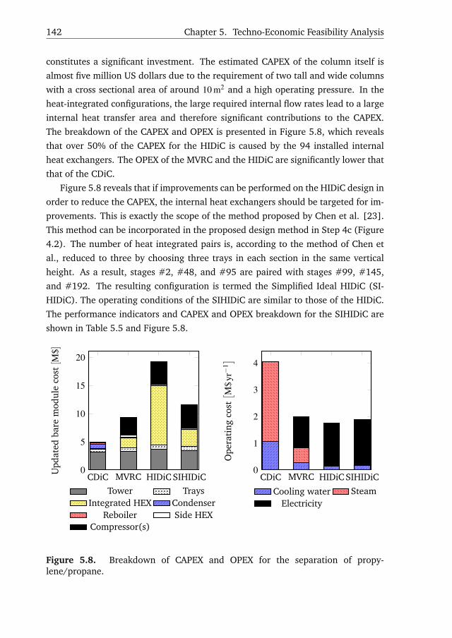
142 Chapter 5. Techno-Economic Feasibility Analysis
constitutes a significant investment. The estimated CAPEX of the column itself is
almost five million US dollars due to the requirement of two tall and wide columns
with a cross sectional area of around 10 m2 and a high operating pressure. In the
heat-integrated configurations, the large required internal flow rates lead to a large
internal heat transfer area and therefore significant contributions to the CAPEX.
The breakdown of the CAPEX and OPEX is presented in Figure 5.8, which reveals
that over 50% of the CAPEX for the HIDiC is caused by the 94 installed internal
heat exchangers. The OPEX of the MVRC and the HIDiC are significantly lower that
that of the CDiC.
Figure 5.8 reveals that if improvements can be performed on the HIDiC design in
order to reduce the CAPEX, the internal heat exchangers should be targeted for im-
provements. This is exactly the scope of the method proposed by Chen et al. [23].
This method can be incorporated in the proposed design method in Step 4c (Figure
4.2). The number of heat integrated pairs is, according to the method of Chen et
al., reduced to three by choosing three trays in each section in the same vertical
height. As a result, stages #2, #48, and #95 are paired with stages #99, #145,
and #192. The resulting configuration is termed the Simplified Ideal HIDiC (SI-
HIDiC). The operating conditions of the SIHIDiC are similar to those of the HIDiC.
The performance indicators and CAPEX and OPEX breakdown for the SIHIDiC are
shown in Table 5.5 and Figure 5.8.
CDiC MVRC HIDiC SIHIDiC0
5
10
15
20
Upd
ated
bare
mod
ule
cost
[M$]
Tower TraysIntegrated HEX Condenser
Reboiler Side HEXCompressor(s)
CDiC MVRC HIDiC SIHIDiC0
1
2
3
4
Ope
rati
ngco
st[ M
$yr−
1]
Cooling water SteamElectricity
Figure 5.8. Breakdown of CAPEX and OPEX for the separation of propy-lene/propane.
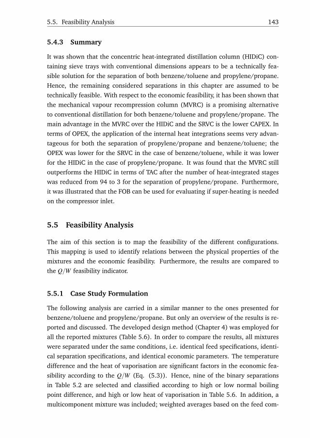
5.5. Feasibility Analysis 143
5.4.3 Summary
It was shown that the concentric heat-integrated distillation column (HIDiC) con-
taining sieve trays with conventional dimensions appears to be a technically fea-
sible solution for the separation of both benzene/toluene and propylene/propane.
Hence, the remaining considered separations in this chapter are assumed to be
technically feasible. With respect to the economic feasibility, it has been shown that
the mechanical vapour recompression column (MVRC) is a promising alternative
to conventional distillation for both benzene/toluene and propylene/propane. The
main advantage in the MVRC over the HIDiC and the SRVC is the lower CAPEX. In
terms of OPEX, the application of the internal heat integrations seems very advan-
tageous for both the separation of propylene/propane and benzene/toluene; the
OPEX was lower for the SRVC in the case of benzene/toluene, while it was lower
for the HIDiC in the case of propylene/propane. It was found that the MVRC still
outperforms the HIDiC in terms of TAC after the number of heat-integrated stages
was reduced from 94 to 3 for the separation of propylene/propane. Furthermore,
it was illustrated that the FOB can be used for evaluating if super-heating is needed
on the compressor inlet.
5.5 Feasibility Analysis
The aim of this section is to map the feasibility of the different configurations.
This mapping is used to identify relations between the physical properties of the
mixtures and the economic feasibility. Furthermore, the results are compared to
the Q/W feasibility indicator.
5.5.1 Case Study Formulation
The following analysis are carried in a similar manner to the ones presented for
benzene/toluene and propylene/propane. But only an overview of the results is re-
ported and discussed. The developed design method (Chapter 4) was employed for
all the reported mixtures (Table 5.6). In order to compare the results, all mixtures
were separated under the same conditions, i.e. identical feed specifications, identi-
cal separation specifications, and identical economic parameters. The temperature
difference and the heat of vaporisation are significant factors in the economic fea-
sibility according to the Q/W (Eq. (5.3)). Hence, nine of the binary separations
in Table 5.2 are selected and classified according to high or low normal boiling
point difference, and high or low heat of vaporisation in Table 5.6. In addition, a
multicomponent mixture was included; weighted averages based on the feed com-

144 Chapter 5. Techno-Economic Feasibility Analysis
position were used to estimate the physical properties of the mixture (α = 1.72,
λ = 44.43kJmol−1, and ∆Tnb = 22.75K, CVP = 0.1402kJmol−1 K−1). This is a simple
consideration, as the classification parameters are not dimensionless and because
they are correlated. However, these parameters are still found useful as classifica-
tion parameters since they are readily available. A common set of feed specifica-
Table 5.6. Considered mixtures for separation. Normal boiling point differ-ence: High when ∆Tnb ≥ 10K, otherwise low. Heat of vaporisation: High whenλ ≥ 33kJmol−1, otherwise low.
Mixture VLE model Classification
Liquid Vapour ∆Tnb λ
m-Xylene/o-xylene Ideal Ideal Low HighIsopentane/n-pentane Ideal Ideal Low LowPropylene/propane SRK SRK Low LowMethanol/ethanol Ideal Ideal High HighAcetic acid/acetic acid anhydride UNIQUAC Ideal High HighEthanol azeotrope/water* UNIFAC Ideal High HighBenzene/toluene Ideal Ideal High HighMethanol/water UNIFAC Ideal High HighBenzene/ethylbenzene Ideal Ideal High High9-Aromatics† Ideal Ideal High High* mole fraction specifications were normalised by 0.87 (azeotropic point)† 9-component mixture from Table 4.8, the feed composition was chosenas z1 = 0.005, zi = 0.1244 for i = 2,3, . . . ,9 with i = 2,3,4,5 representing theC8 fraction and i = 6,7,8,9 representing the heavy fraction.
tions, separation specifications and model parameters is summarised in Table 5.7.
In the case of the azeotropic ethanol/water system, the feed composition and the
product specifications were normalised by 0.87, which is the composition of the
ethanol/water azeotrope. Furthermore, for the mixture of 9 aromatic components,
the product purity specifications applied to the light C8 fraction and the heavy C9
fraction. The fact that all separations have common economic parameters enables
fair comparative studies of the feasibilities among the configurations. In addition,
by maintaining the feed and product specifications identical, the effect of the phys-
ical behaviours of the mixtures on the feasibility is isolated. All the configurations
of Figure 3.1 are considered, namely the CDiC, the MVRC, the HIDiC, and SRVC.
5.5.2 Design Trends
All the obtained designs are presented in Table 5.8. In Figure 5.9, the correlations
between the major design variables and the corresponding physical parameters of

5.5. Feasibility Analysis 145
the mixtures are presented, i.e. the relative volatility (α), the normal boiling point
difference (∆Tnb), and the mean heat of vaporisation (λ).
It appears in Figure 5.9 that all the design variables except CRext,SRVC are corre-
lated with the normal boiling point difference. The propylene/propane separation
is an outlier due to the non-ideal vapour phase. No significant correlations between
the heat of vaporisation and any of the design variables is observed. The correla-
tions between the relative volatilities and the design variables are not as significant
as the normal boiling point differences.
A noticeable observation is the following. The azeotropic ethanol/water mixture
HIDiC design was sensitive to the selection of the compression ratio in the sense that
the minimum temperature driving force was sensitive to the compression ratio. This
observation might indicate challenges w.r.t. operation of such HIDiC. The reason for
this particular sensitivity is because the top product is an azeotrope. Thus, when
the rectifying section pressure is increased by increasing the compression ratio, the
azeotropic point is slightly affected. Hence, low-boiling azeotrope mixtures might
be challenging to realise in an HIDiC.
Based on the observed correlations in Figure 5.9, simple expressions for the
required total heat exchange areas and compression ratios for the HIDiC and the
MVRC can be formulated as:
CRint = 0.0381∆Tnb +1.5936 (R2 = 0.6768) (5.13)
CRext = 0.0642∆Tnb +1.7236 (R2 = 0.7778) (5.14)
∑n
Aint,n = 128,043∆Tnb−1.75 (R2 = 0.9455) (5.15)
Aext = 17,029∆Tnb−0.838 (R2 = 0.9336) (5.16)
The applications of these simple relations cover separations by an HIDiC or an
MVRC of a pseudo-binary mixture into two pure components. These expressions
can be useful in order to carry out preliminary evaluation of a given configuration.
Furthermore, an important observation is that there is no significant relation be-
tween the shape of the temperature profiles and the design variables. Illustrations
of all the temperature profiles are not provided. But for the separation of ethanol
azeorope/water, a temperature pinch is observed for the lowest heat-integrated pair
rather than in the middle of the heat-integrated part of the column, which is the case
of benzene/toluene (Figure 5.3). A similar temperature pinch location is observed
in the separation of methanol/water. Note in Table 5.8 that the presented case
studies cover cases with equally large column sections (e.g. isopentane/n-pentane)
and column sections of different sizes (e.g. ethanol azeotrope/water). Hence, it
is assumed that this present analysis covers the cases of the analysis related to the

146 Chapter 5. Techno-Economic Feasibility Analysis
temperature profiles by Shenvi et al. [142].

5.5. Feasibility Analysis 147
Table 5.7. Feed specifications, purity specifications, and model parameters em-ployed for the feasibility analysis (unless otherwise stated).
Class Parameter Unit Value
Feed and separation specificationsFeed Flow rate mols−1 83.3
Light component molefraction
- 0.50
Pressure kPa 101.3Temperature Saturated
Distillate Light component molefraction
- 0.995
Bottoms Heavy component molefraction
- 0.995
Model parametersInternal heatexchanger
Heat transfer coefficient kWm−2 K−1 0.60
General Electricity price $kWh−1 0.14Steam (Psteam > 200kPa) $t−1 1.99 + 16.2(Psteam −
101.3kPa)0.05
Cooling water (at300 K)
$t−1 0.080
Year - 2012Project life time yr 5Service factor - 0.904Materials - Carbon steel
Tray Pressure drop kPa 0.70Efficiency - 0.80Flooding factor - 0.80Void fraction - 0.75Type - SieveSpacing mm 609.60 (24")
Condenser Water temperature in-crease
K 5.0
Heat transfer coefficient kWm−2 K−1 0.60Type - Floating head
Reboiler Heat transfer coefficient kWm−2 K−1 1.420Difference betweensteam and reboilertemperature
K 10
Type - Kettle reboilerCompressor Isentropic efficiency - 0.80
Motor efficiency - 0.90Type - Centrifugal/motor

148 Chapter 5. Techno-Economic Feasibility Analysis
Table 5.8. Design specifications for the ten considered separations (Table 5.6).
Separation Config. Aint CRint Aext CRext Nrct Nstrm2 - m2 - - -
m-Xylene/o-xylene CDiC 0 1 0 1 101 100MVRC 0 1 6325 3.01 100 101HIDiC 93.7 2.07 0 1 100 101
Isopentane/n-pentane
CDiC 0 1 0 1 59 59
MVRC 0 1 2441 2.01 59 59HIDiC 50.75 1.78 0 1 59 59MVRC 45.5 1.80 53.5 1.25 63 63
Propylene/propane See Table 5.4
Methanol/ethanol CDiC 0 1 0 1 32 32MVRC 0 1 1953 2.773 32 32HIDiC 37.1 2.23 0 1 38 38SRVC 37.1 2.23 326 1.25 38 38
Acetic acid/acetic CDiC 0 1 0 1 23 30acid anhydride MVRC 0 1 1389 2.81 23 30
HIDiC 30.6 2.36 0 1 29 36SRVC 30.6 2.36 216 1.20 29 36
Ethanol CDiC 0 1 0 1 47 8azeotrope/water MVRC 0 1 1771 3.42 47 8
HIDiC 88.2 2.48 0 1 47 8SRVC 88.2 2.48 353.5 1.24 47 8
Benzene/toluene CDiC 0 1 0 1 19 17MVRC 945 3.26 0 1 19 17HIDiC 19.3 2.46 0 1 25 23SRVC 19.3 2.46 374 1.31 25 23
Methanol/water CDiC 0 1 0 1 30 6MVRC 0 1 902 4.78 30 6HIDiC 24.8 3.90 0 1 30 6SRVC 24.8 3.90 397.5 1.11 30 6
Benzene/ethylbenzene CDiC 0 1 0 1 10 10MRVC 0 1 553 5.21 10 10HIDiC 8.02 3.32 0 1 12 12SRVC 8.02 3.32 365 1.55 12 12
Aromatics CDiC 0 1 0 1 38 38MRVC 0 1 2424 2.897 38 38HIDiC 47.2 2.20 0 1 50 50SRVC 47.2 2.202 208 1.40 50 50
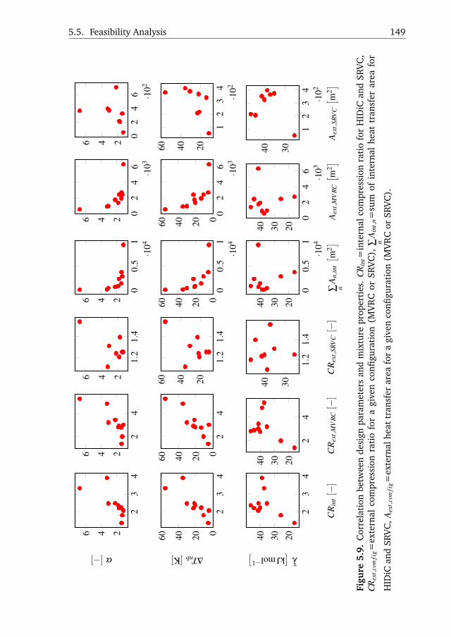
5.5. Feasibility Analysis 149
23
4
246α[−]
24
246
1.2
1.4
246
00.
51
·104
246
02
46 ·103
246
02
46 ·1
02
246
23
40204060
∆Tnb[K]
24
0204060
1.2
1.4
204060
00.
51
·104
0204060
02
46 ·103
0204060
12
34
·102
204060
23
4
203040
CR
int[−
]
λ[kJmol−1]
24
203040
CR
ext,
MV
RC[−
]
1.2
1.4
3040
CR
ext,
SRV
C[−
]
00.
51
·104
203040
∑ nA
n,in
t[ m
2]0
24
6 ·103
203040
Aex
t,M
VRC[ m
2]1
23
4·1
02
3040
Aex
t,SR
VC[ m
2]Fi
gure
5.9.
Cor
rela
tion
betw
een
desi
gnpa
ram
eter
san
dm
ixtu
repr
oper
ties
.CR
int=
inte
rnal
com
pres
sion
rati
ofo
rH
IDiC
and
SRV
C,
CRex
t,co
nfi
g=ex
tern
alco
mpr
essi
onra
tio
for
agi
ven
confi
gura
tion
(MV
RC
orSR
VC
),∑ n
Ain
t,n=
sum
ofin
tern
alhe
attr
ansf
erar
eafo
r
HID
iCan
dSR
VC
,Aex
t,co
nfi
g=ex
tern
alhe
attr
ansf
erar
eafo
ra
give
nco
nfigu
rati
on(M
VR
Cor
SRV
C).
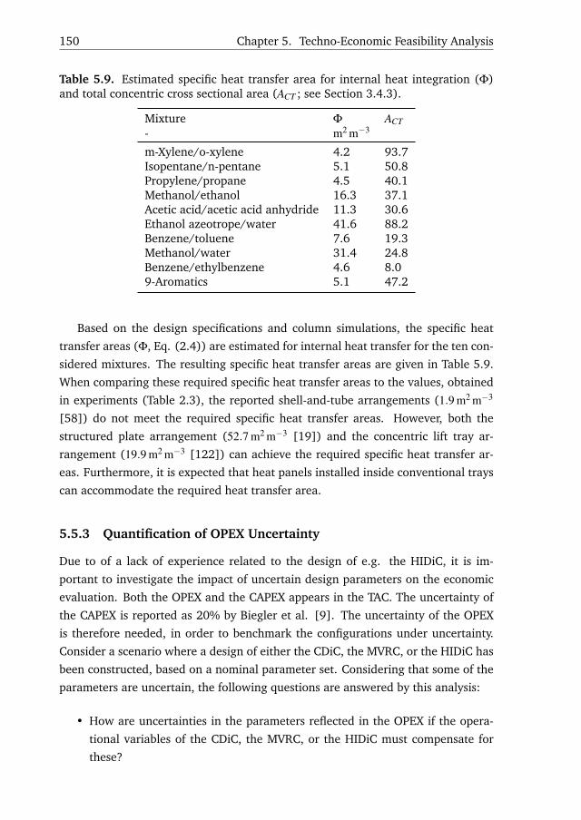
150 Chapter 5. Techno-Economic Feasibility Analysis
Table 5.9. Estimated specific heat transfer area for internal heat integration (Φ)and total concentric cross sectional area (ACT ; see Section 3.4.3).
Mixture Φ ACT- m2 m−3
m-Xylene/o-xylene 4.2 93.7Isopentane/n-pentane 5.1 50.8Propylene/propane 4.5 40.1Methanol/ethanol 16.3 37.1Acetic acid/acetic acid anhydride 11.3 30.6Ethanol azeotrope/water 41.6 88.2Benzene/toluene 7.6 19.3Methanol/water 31.4 24.8Benzene/ethylbenzene 4.6 8.09-Aromatics 5.1 47.2
Based on the design specifications and column simulations, the specific heat
transfer areas (Φ, Eq. (2.4)) are estimated for internal heat transfer for the ten con-
sidered mixtures. The resulting specific heat transfer areas are given in Table 5.9.
When comparing these required specific heat transfer areas to the values, obtained
in experiments (Table 2.3), the reported shell-and-tube arrangements (1.9 m2 m−3
[58]) do not meet the required specific heat transfer areas. However, both the
structured plate arrangement (52.7 m2 m−3 [19]) and the concentric lift tray ar-
rangement (19.9 m2 m−3 [122]) can achieve the required specific heat transfer ar-
eas. Furthermore, it is expected that heat panels installed inside conventional trays
can accommodate the required heat transfer area.
5.5.3 Quantification of OPEX Uncertainty
Due to of a lack of experience related to the design of e.g. the HIDiC, it is im-
portant to investigate the impact of uncertain design parameters on the economic
evaluation. Both the OPEX and the CAPEX appears in the TAC. The uncertainty of
the CAPEX is reported as 20% by Biegler et al. [9]. The uncertainty of the OPEX
is therefore needed, in order to benchmark the configurations under uncertainty.
Consider a scenario where a design of either the CDiC, the MVRC, or the HIDiC has
been constructed, based on a nominal parameter set. Considering that some of the
parameters are uncertain, the following questions are answered by this analysis:
• How are uncertainties in the parameters reflected in the OPEX if the opera-
tional variables of the CDiC, the MVRC, or the HIDiC must compensate for
these?

5.5. Feasibility Analysis 151
• What is the variance of the estimated OPEX for each configuration?
• Which uncertain parameters have the most significant contribution to the vari-
ance?
The uncertain parameters are assumed to be uniformly distributed. The uncertain
parameters and their bounds are listed below:
• Heat of vaporisation, 0.90 λ0 ≤ λ ≤ 1.10 λ0
• Tray pressure drop, 0.80 ∆P0 ≤ ∆P≤ 1.20 ∆P0
• Overall heat transfer coefficient, 0.80 Uihx,0 ≤Uihx ≤ 1.20 Uihx,0
• Constant pressure heat capacity of the vapour, 0.90 CVP,0 ≤CV
P ≤ 1.10 CVP,0
• Ratio of steam price to electricity price, 0.80(Selectricity/Ssteam)0≤ (Selectricity/Ssteam)≤1.20(Selectricity/Ssteam)0.
The nominal uncertain parameters (given by the subscript "0"), the remaining pa-
rameters, and the common design variables are listed in Table 5.10.
Table 5.10. Nominal input and parameters for the two classes of mixtures.
Parameter Unit Value
Pstr kPa 101.3λ kJmol−1 33Tnb,1 K 350Ssteam $kJ−1 10.4 ·10−6
∆P0 kPa 0.70Uihx,0 kWm−2 K−1 0.60CV
P,0 kJmol−1 K−1 0.070(Selectricity/Ssteam)0 - 3.8
Two mixtures with different normal boiling point differences were considered
as this parameter was identified as the must important physical parameter (Section
5.5.2): A mixture with a large normal boiling point difference (∆Tnb = 30) and a
mixture with a low normal boiling point difference (∆Tnb = 5.0). The number of
stages were calculated using the Fenske-Underwood-Gilliland procedure based on
the nominal values listed in Table 5.11. The reflux-to-minimum-reflux ratio was
chosen as 1.05. The designs were carried out such that the compression ratios
(CR) were adjusted to satisfy the minimum temperature driving force condition in
Eq. (4.4), and such that heat transfer areas (A) were adjusted to minimise conven-
tional utilities. The conventional utilities are minimised by imposing the constraint

152 Chapter 5. Techno-Economic Feasibility Analysis
min([Lcnd ,Vrbl ]) = 0 for the HIDiC and min([Qcnd ,Qrbl ]) = 0 for the MVRC. For all
configurations, the remaining degrees of freedom (Lcnd and Vrbl) were chosen such
that the purity constraints were fulfilled. The feed specifications and economic pa-
rameters are identical of those in Table 5.7. A Monte Carlo sample size of Np = 1000
Table 5.11. Nominal design for the two classes of mixtures.
∆T Configuration Nrct Nstr Lcnd/F Vrbl/F CR AK - - - - - - m2
30 CDiC 19 18 0.696 1.20 1 030 MVRC 19 18 0.696 1.20 3.44 109630 HIDiC 19 18 0 0.50 2.53 24.9
5.0 CDiC 90 89 5.92 6.42 1 05.0 MVRC 90 89 5.92 6.42 2.98 58855.0 HIDiC 90 89 0 0.50 2.07 75.3
was used for each design (rows in Table 5.11) leading to 6000 column simulations.
For every sample, a new set of input variables (Lcnd ,Vrbl ,CR) were obtained in order
to satisfy the purity constraints and minimum utility constraints. Based on the new
set of input variables, the OPEX was calculated. The resulting OPEX estimates are
illustrated in Figure 5.10. The OPEX of CDiC is relatively unaffected by the uncer-
tain parameters and therefore the variance is low. It can be concluded with 95%
confidence that the OPEX is lower of the MVRC than the HIDiC for the wide-boiling
mixture. However, for the close-boiling mixture, the confidence intervals overlap.
The obtained standard deviations for the 30 K mixture are 6.3% for the MVRC and
4.2% for the HIDiC. The obtained standard deviations for the 5 K mixture are 12.5%
for the MVRC and 10.7% for the HIDiC.
The uncertain parameters, which are responsible for the variances, are identified
by the global sensitivity analysis (Section 5.2.3). The obtained SRC values are
plotted in Figure 5.11. As the sums of the SRC’s do not add up to one for the CDiC,
no linear correlation between the uncertain parameters and the OPEX estimates
could be obtained. This is believed to be due to the fact that only the latent heat of
vaporisation affects the OPEX of the CDiC. The relative significance of the uncertain
parameters are represented by the magnitude of the SRC values. Thus, the ratio
between the electricity and the steam prices is the dominating parameter. In the
MVRC, the tray pressure drop is also a significant uncertain parameter, while the
overall heat transfer coefficient is significant for the HIDiC. The heat of vaporisation
does not have a significant impact on the uncertainties.

5.5. Feasibility Analysis 153
CDiC MVRC HIDiC
0.6
0.8
1µ = 1.00
σ = 0.00
µ = 0.608
σ = 0.038
µ = 0.812
σ = 0.034
Configuration
OPE
X[ M
$yr−
1]∆Tnb = 30K
CDiC MVRC HIDiC
2
3
4
5
µ = 5.38
σ = 0.066
µ = 2.88
σ = 0.36 µ = 2.43
σ = 0.26
Configuration
OPE
X[ M
$yr−
1]
∆Tnb = 5.0K
Figure 5.10. OPEX estimate for the CDiC, the MVRC and the HIDiC performingseparations of two different mixtures under uncertain design parameters. The errorbars represent 5% and 95% confidence intervals. Expectation (µ) and standarddeviation σ are given in [M$yr−1].
5.5.4 Benchmarking
The remaining task is to relate the economic feasibility of the considered configu-
rations for the ten case studies to the physical parameters. Based on the conclusion
from the previous section, the major design variables are correlated with the nor-
mal boiling point differences (Eqs. (5.13)-(5.16)). Hence, such correlation is also
expected for the economic feasibility.
An uncertainty in the CAPEX of 20% is assumed [9]. The relative standard de-
viations in the OPEX for two separations of varying ∆Tnb were obtained in Section
5.5.3. For each configurations, a linear correlation between the relative standard
deviation and ∆Tnb was used to estimate the uncertainty of the OPEX. As the SRVC
was not considered in the uncertainty analysis, the uncertainty of its OPEX is as-
sumed to be identical to that of the HIDiC. When standard deviations below zero
were obtained by the linear correlation, these were fixed at zero. The uncertainty
of the TAC is thus obtained by combining the contributions from the CAPEX and
OPEX. The resulting uncertain TAC’s for different mixtures and configurations are
illustrated in Figure 5.12. It can be concluded that the MVRC outperforms the con-
sidered configurations in most of the cases. A similar conclusion was reported by
Harwardt and Marquardt [51].
When plotting the TAC of the resulting configurations for the normal boiling
point differences, trends amond the binary separations are obtained for the dif-
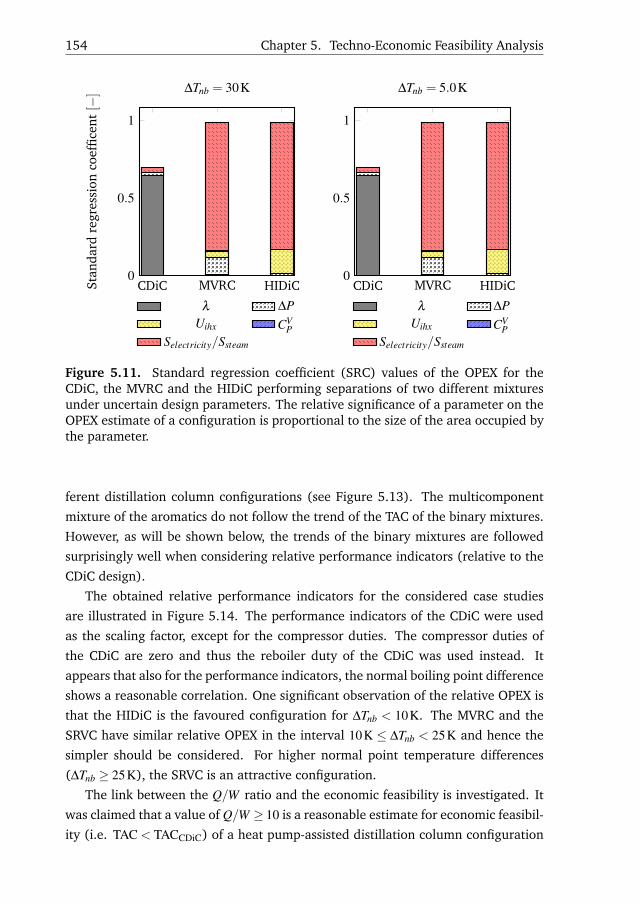
154 Chapter 5. Techno-Economic Feasibility Analysis
CDiC MVRC HIDiC0
0.5
1
Stan
dard
regr
essi
onco
effic
ent[−
] ∆Tnb = 30K
λ ∆PUihx CV
PSelectricity/Ssteam
CDiC MVRC HIDiC0
0.5
1
∆Tnb = 5.0K
λ ∆PUihx CV
PSelectricity/Ssteam
Figure 5.11. Standard regression coefficient (SRC) values of the OPEX for theCDiC, the MVRC and the HIDiC performing separations of two different mixturesunder uncertain design parameters. The relative significance of a parameter on theOPEX estimate of a configuration is proportional to the size of the area occupied bythe parameter.
ferent distillation column configurations (see Figure 5.13). The multicomponent
mixture of the aromatics do not follow the trend of the TAC of the binary mixtures.
However, as will be shown below, the trends of the binary mixtures are followed
surprisingly well when considering relative performance indicators (relative to the
CDiC design).
The obtained relative performance indicators for the considered case studies
are illustrated in Figure 5.14. The performance indicators of the CDiC were used
as the scaling factor, except for the compressor duties. The compressor duties of
the CDiC are zero and thus the reboiler duty of the CDiC was used instead. It
appears that also for the performance indicators, the normal boiling point difference
shows a reasonable correlation. One significant observation of the relative OPEX is
that the HIDiC is the favoured configuration for ∆Tnb < 10K. The MVRC and the
SRVC have similar relative OPEX in the interval 10K ≤ ∆Tnb < 25K and hence the
simpler should be considered. For higher normal point temperature differences
(∆Tnb ≥ 25K), the SRVC is an attractive configuration.
The link between the Q/W ratio and the economic feasibility is investigated. It
was claimed that a value of Q/W ≥ 10 is a reasonable estimate for economic feasibil-
ity (i.e. TAC < TACCDiC) of a heat pump-assisted distillation column configuration

5.6. Conclusion 155
[130]. Based on the result in Figure 5.15, this simple consideration holds well for
the HIDiC, since the relative TAC, according to the trend, is below 1 after around
Q/W = 10. For the MVRC and the SRVC, the plot indicates that these configurations
are preferred in terms of TAC for all mixtures with Q/W ≥ 0.
5.6 Conclusion
A techno-economic analysis of heat-integrated distillation columns has been pre-
sented in this chapter. Four configurations were considered, namely the conven-
tional distillation column (CDiC), the mechanical vapour recompression column
(MVRC), the heat-integrated distillation column (HIDiC), and the secondary re-
flux and vaporisation column (SRVC). It has been illustrated by simulation of the
separation of benzene/toluene that it is possible, by using heat panels, to realise
a HIDiC. Detailed economic analysis of the separations of benzene/toluene and
propylene/propane showed that the capital expenditure of configurations with in-
ternal heat integration comprises a significant drawback to such configurations.
Hence, the reductions in the operating expenses are difficult to justify when con-
sidering the significant capital investment. Significant reductions in the operat-
ing expenses were, however, achieved by the HIDiC for the separation of propy-
lene/propane.
A comprehensive study of nine binary mixtures and one multicomponent mix-
ture being separated in the four different distillation configurations was conducted
and analysed w.r.t. economic feasibility. The presented design method was success-
fully applied to the ten separations. The difference in normal boiling points was
found to be the determining parameter for the feasibility. A measure for the heat
required for distillation per work required (Q/W) was evaluated. It was found that
economic feasibility for any of the three heat-integrated distillation configurations
(MVRC, HIDiC, SRVC) was achieved for Q/W ≥ 0.
The completely heat-integrated SRVC performs the best in terms of OPEX, second-
law efficiency, and water consumption with only a slightly increased CAPEX com-
pared to the HIDiC. Interestingly, the following intervals of the normal boiling dif-
ferences are identified for choosing the preferred configuration among the HIDiC
or MVRC in terms of OPEX:
• ∆Tnb < 10K: The HIDiC
• 10K≤ ∆Tnb: The MVRC
These relations are simplified but they provide actual quantifications of the limits,
which divide the optimal solutions of the heat-integrated distillation configurations.

156 Chapter 5. Techno-Economic Feasibility Analysis
Considering the large expected uncertainties in the CAPEX estimates, the favourable
OPEX in the HIDiC for ∆Tnb < 10K justifies the need for dynamic analyses in the
subsequent chapters.
All performance indicators, as well as the design variables, correlate surprisingly
well with the normal boiling point differences. Therefore, correlations for estimat-
ing the total required heat exchanger area and compression ratio for the MVRC and
the HIDiC were proposed. These are not only useful as preliminary estimates of
the operating and capital expenses, but also for good estimates for the conceptual
design of such configurations. In addition, it was found that the compressor duty of
a heat pump-assisted distillation column configuration usually lies within 10-15%
of the reboiler duty of a corresponding conventional distillation column.
Finally, uncertainty and sensitivity analysis showed that, when building an MVRC
or an HIDiC, the operating expenses are subject to a large uncertainty for close-
boiling separations with a relative standard deviation above 10%. The most sig-
nificant uncertain parameter is the ratio between the cost of energy supplied by
steam over the cost of energy supplied as electricity. The second-most significant
parameters are the tray pressure drop for the MVRC and the overall heat transfer
coefficient for the HIDiC.

5.6. Conclusion 157
CDiCM
VRCHID
iCSR
VC8
1012
TAC[ M
$yr−
1] m-Xylene/o-xylene
CDiCM
VRCHID
iCSR
VC
3
4
Isopentane/n-pentane
CDiCM
VRCHID
iCSR
VC3456
TAC[ M
$yr−
1] Propylene/propane
CDiCM
VRCHID
iCSR
VC1.5
22.5
3Methanol/ethanol
CDiCM
VRCHID
iCSR
VC1.5
2
2.5
TAC[ M
$yr−
1] Acetic acid/Acetic anhydride
CDiCM
VRCHID
iCSR
VC1.5
2
2.5
Azeotropic ethanol/water
CDiCM
VRCHID
iCSR
VC1.21.41.61.8
TAC[ M
$yr−
1] Benzene/toluene
CDiCM
VRCHID
iCSR
VC1
1.21.41.6
Methanol/water
CDiCM
VRCHID
iCSR
VC1
1.21.4
TAC[ M
$yr−
1] Benzene/ethylbenzene
CDiCM
VRCHID
iCSR
VC3
3.54
4.5
9-Aromatics
Figure 5.12. Benchmarking of the four distillation column configurations (CDiC,MVRC, HIDiC, and SRVC) w.r.t. TAC. The TAC=CAPEX/5+OPEX (annual basis),which accounts for uncertainty in OPEX and CAPEX.

158 Chapter 5. Techno-Economic Feasibility Analysis
0 5 10 15 20 25 30 35 40 45 50 55 60
100
101
m-Xylene/o-xylene
Propylene/propane
Isopentane/n-pentane
Methanol/ethanol
Acetic acid/Acetic anhydride
Ethanol azeotrope/water
Benzene/toluene
Methanol/water
Benzene/ethylbenzene
9-Aromatics
Normal boiling point difference [K]
Tota
lann
ualis
edco
st[ M
$yr−
1]CDiCMVRCHIDiCSRVC
Figure 5.13. Correlation between normal boiling point difference and total an-nualised cost (TAC) illustrated using logaritmic axes. The TAC=CAPEX/5+OPEX(annual basis), which accounts for uncertainty in OPEX and CAPEX.

5.6. Conclusion 159
0 20 40 600.2
0.4
0.6
0.8
1
1.2
OPE
X/O
PEX
CD
iC[−
]
0 20 40 60
2
4
6
8
CA
PEX/
CA
PEX
CD
iC[−
]
0 20 40 600
0.2
0.4
0.6
η2n
d[−
]
0 20 40 600
0.2
0.4
0.6f w/
f w,C
DiC
[−]
0 20 40 600
0.2
0.4
0.6
∆Tnb [K]
Qrb
l/Q
rbl,C
DiC
[−]
0 20 40 605 ·10−2
0.1
0.15
0.2
0.25
∆Tnb [K]
E/
Qrb
l,CD
iC[−
]
Figure 5.14. Relative performance indicators. fw is the water consumption, η2ndis the second-law efficiency. Legend: CDiC ( ), MVRC ( ), HIDiC ( ), andSRVC ( ).

160 Chapter 5. Techno-Economic Feasibility Analysis
0 10 20 30 40 50 60 70 80
0.6
0.7
0.8
0.9
1
1.1
1.2
1.3
1.4
Q/W [−]
Rel
ativ
eTA
C[−
]
CDiCMVRCHIDiCSRVC
Figure 5.15. Heat required for distillation per work required (Q/W) and relativetotal annualised cost for the nine binary mixtures. The relative TAC= TAC/TACCDiC.

Chapter6
Stabilising Control
The fundamental problem of obtaining a stabilising control
structure of the concentric heat-integrated distillation column
(HIDiC) is addressed in this chapter. The economic plantwide
control method by Larsson and Skogested was adopted for solv-
ing the problem in a systematic manner [T. Larsson and S. Sko-
gestad. Plantwide control–a review and a new design proce-
dure. Model Ident Control, 21(4):209–240, 2000]. A control
structure of the regulatory control layer is devised, based on
generic considerations and numerical studies. These numerical
studies are based on open-loop considerations and various tools
for controllability analysis. The proposed regulatory control
layer is evaluated by dynamic simulations. The performance,
in terms of setpoint tracking of the controlled variables and the
possibility of entrainment flooding and weeping, was investi-
gated in dynamic simulations. It was concluded that stable op-
eration in both aspects could be achieved for the proposed con-
trol structure. The significance of including pressure dynamics
and accounting for the stabilising control layer is illustrated by
dynamic open-loop simulations, where the obtained responses
are compared to the responses of a simplified model, available
in literature.
This chapter is based on work conducted in collaboration with
Professor Sigurd Skogestad during an exchange period at the
Norwegian University of Science and Technology, Trondheim,

162 Chapter 6. Stabilising Control
Norway.
The results of this chapter were used in an accepted confer-
ence contribution for DYCOPS 2016 [T. Bisgaard, S. Skogestad,
J.K. Huusom, and J. Abildskov. Optimal operation and stabilis-
ing control of the concentric heat-integrated distillation column.
11th IFAC International Symposium on Dynamics and Control ofProcess Systems – Trondheim, Norway, 2016]. Early progress on
this problem was presented during the Nordic Process Control
Workshop 2015 (NPCW19) in Norway.

6.1. Introduction 163
6.1 Introduction
Internal heat transfer takes place in both the heat-integrated distillation column
(HIDiC) and the secondary reflux and vaporisation column (SRVC). These config-
urations show potential favourable economic performances compared to the me-
chanical vapour recompression column (MVRC) and the conventional distillation
column (CDiC). As a result, the dynamic behaviour of the HIDiC is studied in this
chapter, as it is used to represent the behaviour of similar configuration with inter-
nal heat transfer (including the SRVC).
Simple control theory is briefly explained in this section; starting from a presen-
tation of a common control hierarchy in a chemical plant, a systematic economic
plantwide control design procedure, and the purpose of stabilising control.
6.1.1 Control Hierarchy
The control system of a chemical plant can be divided into levels that are performing
actions at different time scales and different partitions of the chemical plant. This
division is called a control hierarchy and is illustrated in Figure 6.1.Simple Rules for Economic Plantwide Control
PLANT
uD
CV2s
CV1s
d
Hou
rsM
inu
tes
Seco
nd
s Regulatory Control
Supervisory Control
ProcessOptimization
F I
P I
T I
ym
ny
y
H2
H
CV2
CV1
(a) Hierarchical time-scale decomposition of the con-trol structure.
MD
MR
MB
PI
FxR
DxD
LT
PC
VB
F0xF0
BxB
TR
A->B
S
TI
(b) Reactor-separator-recycle process flow dia-gram
J = pF F + pQQ− pPP, where: p is the corresponding price, pF F is the sum of the costs of all thefeed streams, pQQ is the cost of all utilities (including energy) and pPP is the sum of the valuesof all products. In this context, we can define two main operational modes: Mode 1 (nominaloperation) where the feeds are given, so the term pF F is fixed. Furthermore, because of givenproduct specifications, this may imply that the product rates P are also fixed. So, to minimize plantoperation cost, we want to minimize the utility costs pQQ. This mode often has an unconstrainedoptimum, since there is a tradeoff between using too much or too little energy. This is the case forour simple example in Mode 1, where the optimal operation is the same as minimizing J = VB,since the energy (boilup) to the column is the only utility; Mode 2 (maximum throughput) that hashigh product prices and low energy prices, so the optimal operation corresponds to maximizingthe product rate P. In general, we have more active constraints in Mode 2 than in Mode 1.
2.2. Economic Plantwide Control description
Any methodology that aims to facilitate the design of an optimal control structure, based on thehierarchical decomposition depicted on Figure 1a, should, independent of the approach, at leastconsider the following structural decisions:
1. Decision 1: Select primary controlled variables CCCVVV 1 for the supervisory control layer orselect HHH. The setpoints CCCVVV 1s link the process optimization with supervisory control layer.
2. Decision 2: Select secondary controlled variables CCCVVV 2 for the regulatory control layer orselect HHH222. The setpoints CCCVVV 2s link the supervisory and regulatory control layers.
3. Decision 3: Locate the throughput manipulator (TPM) location. This is an important step,since it links the top-down and the bottom-up parts of the economic plantwide control.
4. Decision 4: Select pairings for the stabilizing layer controlled variables [CCCVVV 2 ↔ uuuD]
Furthermore, the operational goals should be defined clearly and if possible separated into: i)economic objective ii) stabilization/regulation objectives. One reason for the separation is, thatit is very difficult to measure them in the same units, for example, how much is a gain marginincrease from 2 to 3 worth in dollars?
Skogestad’s procedure clearly distinguishes between the economic control and regulatory controland decomposes the structural decisions, into two parts: the Top-down part, which attempts tofind a slow-time-scale supervisory control structure that achieves a close-to-optimal economic
103
Figure 6.1. Control hierachy [104].
Starting from the top of the control hierarchy, the purpose of the different layers
are as follows [149]:
• Process optimisation: The purpose of this layer is to ensure plantwide opti-

164 Chapter 6. Stabilising Control
mal performance. For example, the objectives of this layer can be achieved by
carrying out plantwide steady state optimisation. The optimal solution from
the plantwide optimisation routine is distributed locally to unit operations
or groups of unit operations and provides the setpoint(s) of the supervisory
control layer.
• Supervisory control layer: This layer provides local, optimising control by
keeping the controlled variables at the setpoint provided from the layer above.
The controlled variables in this layer must be carefully selected in order to en-
sure near-optimal operation when kept at the given setpoint. Hereby, the opti-
misation load is distributed locally in order to reduce the time delay between
the optimisation layer and the process itself. Hence, the control objectives of
this layer are economic rather than stabilisation. The output from this layer
is the setpoints to the lower regulatory layer.
• Regulatory control layer: The role of the regulatory control layer is to pro-
vide fast stabilisation of the process. The setpoints from the supervisory layer
are directly translated into actuator actions in the regulatory layer.
• Plant: The dynamic behaviour of the plant is dictated by the dynamic control
degrees of freedom, which are specified in the above layer. Measurements are
taken on the plant in order to describe the current state of the process. These
measurements are inputs for the above layers.
The scopes of this chapter are related to the investigation of the distillation
column dynamics and the design of the regulatory layer. Stabilisation of a plant
or a process is an essential task and it has not been addressed systematically for a
HIDiC. This work considers control degrees of freedom, which are very similar to
the corresponding actuators in a real HIDiC.
6.1.2 Economic Plantwide Control (Part 1)
A sequential, systematic method for designing the entire control system illustrated
in Figure 6.1 is proposed by Larsson and Skogestad [89, 149]. This method can be
summarised as shown in Figure 6.2. The method is divided into a top-down analy-
sis, which relates to the top layers of the hierarchy in Figure 6.1, and a bottom-up
analysis (Steps 5-7), which relates to the integration of the top-down analysis in
relation to the bottom layers in the hierarchy. Hence, the top-down analysis (Steps
1-3) mainly involves steady state simulation, and the bottom-up part mainly in-
volves dynamic simulation with Step 4 working as the link between the two. An
overview of the method combined with a collection of practical rules are collected

6.1. Introduction 165
1. Define the operationalobjective and constraints
2. Determine the steadystate optimal operation
3. Select the primaryeconomic CVs (CV1)
4. Select the TPM location
5. Select control structurefor the regulatory layer
6. Select control structurefor the supervisory layer
7. Select control struc-ture for the RTO layer
Top-
dow
nA
naly
sis
Bot
tom
-up
Ana
lysi
s
Figure 6.2. Economic plantwide control method [89, 149]. CV: Controlled vari-able; TPM: Throughput manipulator; RTO: Realtime optimisation. Step 4 serves asa transition between the top-down and the bottom-up analyses.
by Minasidis et al. [104]. The work by Minasidis et al. is the basis of the following
introduction of the method. In Step 1, the overall operation objective is formu-
lated, which often is economic. An objective function is formulated reflecting the
operation objective and the associated degrees of freedom are identified. Expected
economic disturbances are also identified in this step. The operation conditions
for every economic disturbance scenario of optimal operation is identified in Step
2 by solving the optimisation problem, which arises from the formulated objective
function. The knowledge gained from the identification of optimal operation is in
Step 3 applied to select the primary controlled variables (CV1). The primary con-
trolled variables are typically controlled in the supervisory layer (see Figure 6.1). In
Step 4, the throughput manipulator (TPM) is selected, which has a significant im-
pact on the decisions related to the following steps. When the TPM is selected, the
bottom-up part starts in Step 5, where the control structure in the regulatory layer
is selected. This selection covers the pairing of the secondary controlled variables

166 Chapter 6. Stabilising Control
(CV1) with the process actuators (uD in Figure 6.1). Following the selection of
regulatory layer in Step 5, a similar selection of the supervisory layer is performed
in Step 7. Thus, the CV1’s are paired with the CV2. The final step is Step 7, in
which the process optimiser is located. This typically consists of a real-optimisation
layer (RTO) that provides the optimal setpoints. In some cases, a well-designed
supervisory layer can make the RTO layer redundant.
6.1.3 Stabilising Control
The concept of stabilising control covers the actions of the regulatory layer, i.e.
the adjustments in process actuators in order to maintain stable operation. Stable
operation means that drifts in operation are avoided. This generally corresponds
to controlling liquid holdups and pressures. Furthermore, the temperature profile
of a distillation column behaves like a drifting variable, as it can be illustrated as
a level between the light components in the top and the heavy components in the
bottom [150]. Thus, abnormal operation caused by composition changes is avoided
by controlling the temperature.
The main objective of the regulatory layer is to provide stabilisation of the plant
in both a mathematical sense (eliminate integrating processes) and a practical sense
(avoid drift in operation). This is realised by stable and robust control, which
should work under all the conditions imposed by the economic supervisory layer.
The regulatory layer is an indispensable part of a plant or unit operation, as stability
is closely related to safety. Another objective of the regulatory layer is to provide
fast control as illustrated in Figure 6.1, which is reflected in the selection of the
controlled variables (CV2) and their pairing with the actuators. A rule of thumb is
formulated by Minasidis et al. [104], which suggests that the pairing of a controlled
and a manipulated variable should be carried out in such a way that the physical
distance between the corresponding measurement and actuator is minimised. This
rule is adopted throughout this chapter and is referred to as the "pair close" rule.
As a single unit operation is the focus rather than that of an entire plant, the
TPM position has no significant importance. As a result, the design of the regulatory
layer can be performed without considering Steps 1-4, based on dynamic analysis
and general guidelines [104]. This approach is applied in this chapter.
6.1.4 Proportional-Integral Control
Proportional-integral-derivative controllers are most often referred to as PID con-
trollers. PID controllers are feedback controllers, which act on a deviation from a
specified setpoint of a controlled variable. In this work, PI controllers have been
6.2. Operation Analysis 167
found sufficient, thereby ignoring the derivative (D) action. The deviation between
the desired setpoint and the measured output is termed the error. The error is
defined as:
e(t) = yset(t)− ym(t) (6.1)
where
e(t) = error of controlled variable k at time t
yset(t) = setpoint of the controlled variable k
ym(t) = measured value of the controlled variable k
The control action, u, can be written in terms of the error:
u(t) = u(t = 0)+Kc
(e(t)+
1τI
∫ t
0e(τ)dτ
)(6.2)
u(t) = controller action
Kc proportional gain (controller tuning parameter)
τI integral gain (controller tuning parameter) [s]The values of Kc and τI can be obtained by using tuning rules. The Skogestad
Internal-mode control method (SIMC) [148] has been adopted in this work. This
method requires only one tuning parameter, the desired closed-loop time constant
(τc), along with a transfer function describing the relation between the manipulated
and the controlled variable. The notation u→ y is used to represent a control loop,
in which u is manipulated to control y.
6.1.5 Case Study
A concentric HIDiC separating benzene/toluene is considered in this chapter. The
considered concentric HIDiC design is summarised in Table 6.1 and the model pa-
rameters are given in Table 5.7. Conventional column sizing has been employed
using the tray dimensional parameters listed in Table 5.1. This design leads to a
gradually increasing rectifying section diameter when moving from the top to the
bottom, while the stripping section diameter is gradually decreasing. The trend in
the column diameter and the column design is illustrated in Figure 6.3. As a result,
the nominal tray liquid holdups vary along the column. Based on the considera-
tions of Section 5.4, it is assumed that a uniform heat transfer area, among the
heat-integrated stages, can be achieved by installing heat panels within the column
structure.
6.2 Operation Analysis
Generic considerations of a general HIDiC are presented, relating to the identifica-
tion of the manipulated and the controlled variables.

168 Chapter 6. Stabilising Control
Table 6.1. Design and nominal operation point if the concentric HIDiC.
Class Specification Unit Value
Feed Flow rate mols−1 83.3Benzene mole fraction - 0.50Pressure kPa 101.3Temperature K 365.3
Distillate Benzene mole fraction - 0.99Bottoms Benzene mole fraction - 0.01Design Trays in the rectifying section - 25
Trays in the stripping section - 23Heat exchange area per tray m2 19.3Column cross sectional area m2 See Figure 5.2Condenser holdup mol 12,550Reboiler holdup mol 22,626Tray holdups (min/max) mol 355 / 1610
Operation Compression ratio - 2.306Feed location pressure kPa 101.3Reflux flow rate mols−1 0.8333Reboiler duty kW 1175
6.2.1 Operational Degrees of Freedom
A general representation of a HIDiC with actuators and indicators is given in Figure
6.4. The indicators are also shown in the figure. The indicators and their selection
will be discussed in more detail below. The number of actuators corresponds to the
number of operational degrees of freedom. These are listed in Table 6.2. Because
the HIDiC is considered an isolated process as part of a plant, the feed flow rate is
not considered as an operation degree of freedom and is hence considered as the
TPM.
The HIDiC considered (Figure 6.4) has seven operational degrees of freedom
reflected in six valves and one compressor setting. Four of the valves are manipu-
lating flow rates directly (V-1, V-2, V-4, and V-6). In a real set-up, the valves V-3 and
V-5 are manipulating the flow rates of cooling water and steam. However, in sim-
ulation it is assumed that these valves can directly manipulate the corresponding
duties of the condenser (Qcnd) and the reboiler (Qrbl), respectively. The operational
degrees of freedom, represented by valves V-1, V-2, V-3, V-4, and V-5, are identical
to those of the conventional distillation column (CDiC). When converting the CDiC
into the HIDiC, three additional operational degrees of freedom arise. First of all,
the introduction of the compressor adds an additional operational degree of free-
dom, the compressor setting (C-1). The compressor setting of a real process could
be its rotational speed, but in this work it is represented by the compressor duty.

6.2. Operation Analysis 169
#2#3#4#5#6#7#8#9
#10#11#12#13#14#15#16#17#18#19#20#21#22#23#24#25#26
Compressor
V-1
V-3
V-2
V-5
V-4
Cooling water
Steam
Bottoms
Distillate
Feed
#1
V-6
C-1ActuatorsV-1: LcndV-2: DV-3: QcndV-4: BV-5: QrblV-6: LintC-1: E
#27
#51
TPM
#33#34#35#36#37#38#39#40#41#42#43#44#45#46#47#48#49#50
#28#29#30
#32#31
Figure 6.3. A concentric HIDiC with actuators separating benzene/toluene.
Ho et al. [55] argue that a pressure regulator valve should be used for controlling
the rectifying section outlet liquid pressure in order to avoid liquid maldistribution
in its entry point in top of the stripping section. However, it is presumed that this
pressure is self-regulating and that a reasonable liquid pressure can be achieved if
the level controller valve and/or the outlet nozzle (entry) are dimensioned appro-
priately. As a result of physically separating the two column sections, the flow rate
of the liquid between the two sections must be regulated, which can be done by
valve V-6. A similar degree of freedom analysis is provided by Ho et al. [55] for
several simpler HIDiC configurations. The difference between the actuators by Ho
et al. and the actuators in Table 6.2, is that Ho et al. used the compressor rotation
speed rather than the duty.

170 Chapter 6. Stabilising Control
Rec
tify
ing
Sec
tio
n
Stri
pp
ing
Sect
ion
Heat Transfer
V-3
LI-2LI-3
LI-1
PI-1PI-2
F, z
B
Vrbl
Qrbl
Lint
Lcnd
D
Qcnd
E
C-1
V-5
V-6
V-4
V-2V-1
TPM
DTI-2
DTI-1
Figure 6.4. Conceptual representation of the HIDiC with actuators and measure-ment indicators.
6.2.2 Identification of Secondary Controlled Variables (CV2)
The secondary controlled variables are identified by analysis of the HIDiC illustrated
in Figure 6.4. Potential drifting variables are identified in a systematic manner using
the guidelines by Minasidis et al. [104]. All selected secondary controlled variables
constitutes CV2. These are listed below:
• Temperature profile: The temperature profile must be controlled, which is
equivalent to controlling one composition in the column. In this work, the
possibility of composition control is left for the economic objectives presented
in Chapter 7. This approach enables the supervisory layer to manipulate the
setpoint of the temperature profile controller. Due to this possible coupling to
the supervisory layer, the temperature control is suggested to be carried out
in the column section containing the more valuable component. Therefore,
the design of the temperature controller is case specific and the following sce-
narios must be considered: The top product is more valuable and the bottom

6.2. Operation Analysis 171
Table 6.2. Identification and classification of degrees of freedom assuming givenfeed flow rate.
Label Operation degrees of freedom Steady state degrees of freedom
V-1 Reflux flow, Lcnd Reflux flow rate, LcndV-2 Distillate flow, D Condenser holdup*, McndV-3 Condenser duty, Qcnd Stripping section pressure, PstrV-4 Bottoms flow, B Reboiler holdup*, MrblV-5 Reboiler duty, Qrbl Boilup flow rate, VrblV-6 Intermediate flow, Lint Intermediate holdup*, MintC-1 Compressor duty Rectifying section pressure, Prct
* No steady state effect
product is more valuabe. In addition to stabilisation, temperature control
provides several benefits as e.g. indirect level control, indirect composition
control, and reduces the interactions in any composition control loops. Since
pressure dynamics are expected to play a significant role in the stabilisation
of a HIDiC, it is proposed to control a temperature difference across a column
section. This provides a simple built-in pressure compensation at an increased
complexity of controller design as two sensors must be located rather than
one. The criteria for selecting the column temperature measurement(s) are
given by Skogestad [150]:
– The location should be within the column rather than at the column
ends,
– control temperature in the column end where composition control is
most important (usually the case for the more valuable product),
– locate the temperature where the steady state sensitivity is large ("maxi-
mum gain rule"),
– for dynamic reasons, one should avoid locating a temperature sensor in
a region with a small temperature change from one stage to the next
(avoid "flat" temperature profile),
– use an input in the same end as the temperature sensor since the tem-
perature loop must be fast, and
– avoid using an input that may saturate.
The sensor for measuring the difference in temperatures is referred to as a
differential temperature indicator (DTI) in Figure 6.4.
• Section Pressures: A pressure is a measure of a vapour holdup and therefore
closely resembles an integrating process. It is expected that the pressures of

172 Chapter 6. Stabilising Control
both column sections, i.e. that of the rectifying section (Prct) and that of the
stripping section (Pstr), must be controlled for stabilisation. A similar, explicit
treatment of the control of the pressures in both column sections has not been
encountered in literature. This might be due to the fact that the pressures do
have some degree of self-regulation. For example, an increase in the rectifying
section pressure leads to an increase in the tray temperatures and therefore
the amount of internal heat integration increases. As heat is removed in the
rectifying section due to heat integration, the pressure decreases as vapour
is condensed. However, as the change in internal heat transfer affects the
separation, the above control layers might prevent it. The pressure stabilisa-
tion gives rise to some valuable analysis of this particular behaviour. Pressure
sensors can in principle be placed in any tray of each section. Hence, the
preferred position is investigated from a stabilisation point of view. The loca-
tion of pressure sensors can also have economic implications [90, 101]. The
pressure sensors are called pressure indicators (PI) in Figure 6.4.
• Liquid holdups: Dynamic holdups act as pure integrators and are therefore
unstable. In most cases, in particular for non-reactive systems, the holdups
do not have impact on the steady state and are therefore not considered.
However, holdups act as buffer tanks in a dynamic system and influence the
time constants of e.g. the composition responses. As a result, these effects are
included in these studies. Similar to conventional distillation, the condenser
holdup (Mcnd) and the reboiler holdup (Mrbl) must be controlled. Due to the
physical separation of the rectifying section and the stripping section, it is not
certain that gravity is used to transport the liquid from the rectifying section
to the stripping section, nor it is certain that the pressure difference between
the sections can stabilise the liquid holdup. Therefore, it is expected that
the bottom holdup of the rectifying section (Mint) must be controlled. The
subscript "int" is used for intermediate as referring to in-between the column
sections. Liquid holdups can be measured directly in the corresponding tanks.
The sensors for measuring the liquid holdups are called level sensors and are
displayed in Figure 6.4 using the abbreviation "LI" for level indicator.
• Liquid pressure: The pressure of the liquid entering the low-pressure strip-
ping section from the high-pressure rectifying section must be controlled such
that the entrance of the liquid in the stripping section does not cause dis-
ruption in entrance location. The pressure of the entering liquid should be
adjusted to approximately that of the pressure of the entrance location.
• Internal hydraulics: In this work, simulations indicated that most HIDiC

6.3. Design of Regulatory Layer 173
designs have no external reflux. A small, but consistent, liquid reflux might
be needed to keep the separation efficiency above a certain limit in the upper
trays. In some cases, this might lead to an economic loss and therefore the
minimum liquid reflux flow rate is a fixed back-off value.
6.3 Design of Regulatory Layer
The design of the regulatory layer denotes the pairing of the manipulated variables
uD with the measurements y of the secondary controlled variables CV2:
uD = [Lcnd ,D,Qcnd ,B,Qrbl ,Lint ,E]T (6.3)
y = [Mcnd ,Mrbl ,Mint ,Prct ,Pstr,∆T,Lcnd ]T (6.4)
Note that the liquid reflux flow rate Lcnd is listed as a measurement in order to
reflect that it is considered as a secondary control variable.
Generally, simple PI controllers (or PID) are desired in the regulatory control
layer. The pairing is done sequentially in the order of the following subsections.
The simple Skogestad IMC (SIMC) rules [148] are employed for tuning of the PI
controllers. Therefore, model identification is carried out on rigorous dynamic re-
sponses in order to obtain low-order transfer functions. The considered transfer
functions are an integrating process, a first-order transfer function, a second-order
transfer function, and a second-order transfer function with numerator dynamic
transfer function. Time delays are included for all the considered transfer func-
tions. The only decision variable related to the tuning is the desired closed-loop
time constant (τc) when a transfer function has been obtained.
6.3.1 Liquid Holdup Control
Based on the "pair-close" rule, the only options for the control of the condenser
holdup is the distillate flow rate (D→Mcnd) and the liquid intermediate flow rate to
control the intermediate holdup (Lint →Mint). The most obvious way of controlling
the reboiler holdup is by the bottoms flow rate (B→Mrbl) rather than by the boil-
up rate, which is dictated by the reboiler duty. Note that the distillate flow rate
is the only option for controlling the condenser holdup. Note that contrary to a
conventional distillation column, the reflux flow rate is close to saturation for the
HIDiC (Lcnd = 0.8333mols−1). Therefore, the liquid reflux flow rate is an infeasible
candidate as the manipulated variable. In this work, it is assumed that the dynamics
of the intermediate holdup is identical to that of the remaining trays. As a result,
the intermediate flow rate is described by the Francis weir formula in Eq. (3.35).
This has a similar response to that of a simple P controller.

174 Chapter 6. Stabilising Control
Actuator dynamics are neglected in this work, so the simple integrating pro-
cesses are obtained:
∆Mcnd(s)∆D(s)
=−1s
(6.5)
∆Mrbl(s)∆B(s)
=−1s
(6.6)
where
s = the independent variable in the Laplace domain
∆ = deviation from steady state
These transfer functions can be derived mathematically as shown in Illustration 6.1.
A value of τc = 120s was considered as a reasonable value, since it is not critical to
keep the holdups tightly controlled.
Illustration 6.1. Derivation of transfer functions for liquid holdup.
Take the example of the condenser. Its total mass balance is
Mcnd
dt=V2−Lcnd−D.
Taking the Laplace transform on both sides and introducing deviation variables
yields:
s∆Mcnd(s) = ∆V2(s)−∆Lcnd(s)−∆D(s),
which leads to:
∆Mcnd(s)∆V2(s)
=1s,
∆Mcnd(s)∆Lcnd(s)
=−1s,
∆Mcnd(s)∆D(s)
=−1s
A similar approach applies to the intermediate holdup and the reboiler holdup.
6.3.2 Pressure and Temperature Control
As the nominal reflux flow rate is expected to be low, the remaining actuators are
Qcnd , Qrbl , and E, which can be used to control Prct , Pstr, and ∆T . Usually, from a
stabilisation point of view, the selection of the location of the pressure sensor is not
important. As a result, the column section pressures are measured in the top of
the column sections. According to the guidelines listed in Section 6.2.2, the con-
trolled temperature should be sensitive to the inputs in steady state and must not be
located at a flat region in the temperature profile. As it was argued to control a tem-
perature difference in the HIDiC, it is proposed to locate a tray i, whose temperature
must be subtracted from the temperature in the top of the rectifying section (T2) if
∆T is located in the rectifying section, or from the temperature in the bottom of the

6.3. Design of Regulatory Layer 175
stripping section (TNS−1) if ∆T is located in the stripping section. These column end
temperature measurements represent the stable part of ∆T , which provides pres-
sure compensation. By considering the steady state gains of step changes in the
potential manipulated variables (Qcnd , Qrbl , and E) in all possible combinations of
∆T = T2−Tk, k = 3,4, . . . ,NF − 1, it was found that the combination ∆T = T2−T17
had the largest gain. Interestingly, the temperature at stage #17 corresponds to the
pinched pair, i.e. the location where the temperature gradient responsible for in-
ternal heat transfer is the smallest (see Figure 5.3). This result appears reasonable,
as simulations have shown that changes in operation can move the pinch location
thereby indicating sensitivity to operational changes. Based on this reflection, the
pinch location is a suitable starting point for defining ∆T for any separation.
A similar analysis was carried out for the case, where the temperature profile
must be controlled in the stripping section. Again, it was found by simulation
that the more sensitive controlled variable is ∆T = T43−T50, which corresponds to
the temperature difference between the heat transfer pinch location (stage #43)
and the bottom of the stripping section (stage #50). When ∆T is evaluated for
both column sections, the rectifying section temperature difference will be denoted
(∆T )rct and the stripping section temperature difference will be denoted (∆T )str.
Typically, in conventional columns, the pressure of the entire column is con-
trolled by the condenser duty. The reason why this is not the case for the HIDiC is
the significant amount of heat integration. The nominal condenser duty is−1240 kW,
while the total nominal amount of heat, exchanged in the rectifying section, is
−2181 kW. Hence, the total amount of internal heat transfer is twice the amount of
the condenser duty. Therefore, significant dynamic interactions are expected. The
individual initial responses of the three controlled variable candidates (Prct , Pstr,
and ∆T ) subject to ±1% step changes in the manipulated variable candidates (Qcnd ,
Qrbl , and E) are illustrated in Figure 6.5. Order transfer functions of as low order
as possible have been fitted to the dynamic responses of the full model. These re-
sponses are illustrated in Figure 6.5. A visual representation of the match between
the fitted responses and the actual reposes is provided in the figure as well. In gen-
eral, the fitted transfer functions were able to describe both the actual dynamics in
the initial responses and to predict the resulting steady states.
When considering both options for controlling the temperature profile (∆(∆T )rct
and ∆(∆T )str), the system matrix G(s) can be represented in the following way:∆Prct
∆Pstr
∆(∆T )rct
∆(∆T )str
= G(s)
∆Qcnd
∆Qrbl
∆E
(6.7)

176 Chapter 6. Stabilising Control
The obtained transfer functions based on the best match can be represented by the
system matrix:
G(s) =
4.444·10−3(24.87s+1)(937.2s+1)(7.351s+1)
3.807·10−3e−3.422s
(935.9s+1)(18.19s+1)5.218·10−3(93.56s+1)e−1.806s
(809.3s+1)(17.25s+1)2.220·10−3e−2.742s
895.1s+11.915·10−3e−5.185s
915.2s+10.8678·10−3(−657.9s+1)(1026s+1)(4.066s+1)
−58.40·10−3(26.77s+1)(1920s+1)(2.265s+1)
6.921·10−3(1285s+1)(2503s+1)(2499s+1)
0.2707·10−3(−17465s+1)e−108.5s
(2819s+1)(356.0s+1)−46.77·10−3(−42.74s+1)e−5.075s
(2364s+1)(21.04s+1)−16.26·10−3(−140.3s+1)(1944s+1)(11.06s+1)
−54.54·10−3(953.5s+1)e−18.18s
(1932s+1)(250.4s+1)
(6.8)
In all transfer function representations, the pressures are given in bar. Both the
initial responses in Figure 6.5 and the obtained transfer functions in Eq. (6.8)
witness the rather complex dynamics of the HIDiC. For example, an inverse re-
sponse is observed in the responses for Pstr when E is changed. Furthermore, the
response of ∆T to changes in E has a small steady state gain but a complicated
dynamic response, which the low-order transfer functions are not able to capture.
The obtained transfer function is a second-order transfer function with numerator
dynamics with inverse response. However, it does not capture the initial response,
which is in the same direction of the final response.
The steady state relative gain array (RGA) [17] can be used to assist in the de-
cision on the pairing of the manipulated and controlled variables for decentralised
control. RGA elements close to unity are preferred and must not be negative. If
temperature control must be carried out in the rectifying section, ∆(∆T )str is omit-
ted in Eq. (6.8) and a 3×3 system matrix (Grct(s)) is obtained. The following RGA
is obtained:
Grct(s = 0) = 10−3
4.4440 3.8070 5.21802.2200 1.9150 0.8678−58.4000 6.9210 0.2707
⇒
ΓΓΓ = Grct ⊗(G−1
rct)T
=
−0.0549 −0.4396 1.49450.1754 1.3192 −0.49450.8795 0.1204 0.0000
The structure of the RGA is identical to Eq. (6.8) with controlled variables in rows
and manipulated variables in columns. The final suggestion for pairing is high-
lighted in the RGA as boldface numbers, which leads to Qcnd → ∆T , Qrbl → Pstr and
E → Prct . The two latter pairings are intuitive, but the former pairing is not. How-
ever, it was found that it should be possible to use the condenser duty for controlling
the temperature profile. These three resulting control loops appear to be feasible
by considering both the steady state RGA and the initial responses (Figure 6.5).
Furthermore, the obtained pairings are in accordance with the "pair close" rule.

6.3. Design of Regulatory Layer 177
A similar analysis of the RGA is carried out for the temperature difference lo-
cated in the stripping section. In this case, the RGA becomes:
G(s = 0) = 10−3
4.4440 3.8070 5.21802.2200 1.9150 0.8678
46.7700 −16.2600 −54.5400
⇒
ΓΓΓ = G⊗(G−1)T
=
0.9089 −1.3934 1.4846−0.6172 2.1090 −0.49180.7083 0.2845 0.0073
A similar pairing is obtained when choosing the pairing resulting in RGA elements
close to unity (indicated in RGA as boldface numbers). It might seem undesirable
to control the stripping section temperature profile with the condenser duty when
having the "pair close" rule in mind. But as illustrated previously, the sum of the
internal heat integration is larger than the condenser duty itself. In fact, the ef-
fect on the opposite section might be at least as significant due the self-regulating
behaviour as discussed in Section 6.2.2. For both locations of ∆T , the dominant
factor for the resulting pairing is the direct coupling between the compressor duty
and the rectifying section pressure. This is illustrated by the significant gain for the
rectifying section pressure compared to the remaining controlled variables, which
is clear in the last column in the steady state gain matrix G(s = 0).A remark on the illustrated dynamic responses for a CDiC in Figure 6.5 is that
these responses have both larger time constants and smaller gains than those of the
HIDiC. For example, the steady state gain matrix is:
GCDiC(s) =
[∆Prct
∆Qcnd
∆Prct∆Qrbl
∆Pstr∆Qcnd
∆Pstr∆Qrbl
]= 10−3
[2.474 2.5152.072 2.245
]
6.3.3 Liquid Pressure and Internals Hydraulics Control
These two control loops will not be considered in this work, as they are not mod-
elled. The liquid preessure of the intermediate liquid flow has no impact on the
model solution as the enthalpy is independent of pressure (see Eq. (3.17)). It was
discussed previously that the liquid reflux should be kept low, but at the same time
it should be kept at a non-zero value in order to keep the top trays wetted. A flow
controller is needed to satisfy this requirement. As the liquid reflux is a model input,
no controller is required in this work.

178 Chapter 6. Stabilising Control
6.3.4 Recommendations and Discussion
A list of the fundamental controllers of a HIDiC constituting the stabilising control
structure in the regulatory layer can be summarised:
• V-6(Lint)→Mint : Level control (LC). The dynamics are not considered in this
work.
• V-1→ Lcnd: Flow control (FC).
• V-2(D)→Mcnd: Level control (LC).
• V-4(B)→Mrbl: Level control (LC).
• V-5(Qrbl)→ Pstr: Pressure control (PC).
• V-3(Qcnd)→ ∆T : Differential temperature control (DTC). Note that this struc-
ture is independent on the location of the measurement of the column tem-
perature profile.
• C-1(E)→ Prct : Pressure control (PC).
The items in the above list are presented in the order of the proposed sequential
tuning procedure. Level controllers have no significant interactions with the re-
maining loops and should therefore be tuned and implemented first. The latter
three loops are sorted according to an increasing desired closed-loop time constant
(τc). Furthermore, the resulting control structures for stabilising a HIDiC for the
two considered cases (distillate or bottoms valuable product) are illustrated in Fig-
ure 6.6. Based on the results, it should be able to design the regulatory control
structure for any HIDiC as most considerations are generic. The control of the
temperature profile based on the temperature measurements of the pinch locations
requires evaluation of several different mixtures. As seen in Chapter 5, it appears
that common separations have a heat transfer pinch location near the middle of
the column sections. According to the previous analysis, the heat-integrated tray,
involved in a heat transfer pinch location in the considered column section, ap-
pears to be a suitable candidate for temperature profile control. This statement is
explored by simulation in the following section.

6.4. Dynamic Evaluations 179
LC
LC
PC
Qcnd
D
E
Mcnd
ΔT
Mrct
Prct
Pstr
Qrbl
B
LC
LC
PC
LC
Qcnd
D
LintE
Mcnd
Mrct
Mrct
Pstr
Qrbl
B
PCPstroptPrctset
FC
LcndLcnd
Lcndopt
CCxDopt
xD
ΔTset
CCxB
Pstrset
xBopt
TDC
LC
LC
PC
PC
LC
Qcnd
D
LintE
Mcnd
Mrct
ΔT
Mrct
Prct
Pstr
Qrbl
B
Prctset
FC
LcndLcnd
Lcndopt
CCxDopt
xD
PC
xB
xBopt
ΔTset
Regulatory
Top valuable (with 2xCA)
Bottom valuable
Pstropt
PC
DTC
Prct
ΔT
DTC
LCLint
Mint
PC
FC
Lcnd
LC
LC
PC
Qcnd
D
E
Mcnd
ΔT
Mrct
Prct
Pstr
Qrbl
B
PC
DTC
LCLint
Mint
FC
Lcnd
(a) Distillate more valuable product,which requires control of the rectifyingsection temperature profile.
LC
LC
PC
Qcnd
D
E
Mcnd
ΔT
Mrct
Prct
Pstr
Qrbl
B
LC
LC
PC
LC
Qcnd
D
LintE
Mcnd
Mrct
Mrct
Pstr
Qrbl
B
PCPstroptPrctset
FC
LcndLcnd
Lcndopt
CCxDopt
xD
ΔTset
CCxB
Pstrset
xBopt
TDC
LC
LC
PC
PC
LC
Qcnd
D
LintE
Mcnd
Mrct
ΔT
Mrct
Prct
Pstr
Qrbl
B
Prctset
FC
LcndLcnd
Lcndopt
CCxDopt
xD
PC
xB
xBopt
ΔTset
Regulatory
Top valuable (with 2xCA)
Bottom valuable
Pstropt
PC
DTC
Prct
ΔT
DTC
LCLint
Mint
PC
FC
Lcnd
LC
LC
PC
Qcnd
D
E
Mcnd
ΔT
Mrct
Prct
Pstr
Qrbl
B
PC
DTC
LCLint
Mint
FC
Lcnd
(b) Bottoms more valuable product, whichrequires control of the stripping sectiontemperature profile.
Figure 6.6. Regulatory layer control structures depending on product values. LC:Level controller, PC: Pressure controller, DTC: Differential temperature controller,FC: Flow controller.
6.4 Dynamic Evaluations
In this section, the developed regulatory control layer structure is evaluated by
simulation. Benzene/toluene is used as the model feed mixture, while it is assumed
that the distillate is the more valuable product. Hence, the evaluation concerns the
control structure shown in Figure 6.6(a).
6.4.1 Tuning
Sequential tuning was carried out in the order, displayed in Table 6.3 (starting
from the top). The table provides the identified first-order models, the desired
closed-loop time constant, and the resulting controller parameters. Desired closed-

180 Chapter 6. Stabilising Control
loop time constants were chosen in the order of minutes because large actions are
undesired in the pressure control loops. In addition, numerical convergence issues
in the differential equation solver were encountered for more tightly controlled
pressure loops.
The manipulation of the steam supply, and hence the reboiler duty, is reason-
ably fast. Therefore, the desired closed-loop time constant of this loop is chosen
as τc,Qrbl→Pstr = 90s. The rectifying section pressure control loop were chosen to be
the slowest as it is desirable to run the compressor with as few operational changes
as possible (τc,E→Prct = 180s). Finally, the desired closed-loop time constant of the
loop involving the condenser duty is chosen as τc,Qcnd→∆T = 120s since Skogestad
[150] recommends to have a rather fast temperature controller. A benefit of choos-
ing the largest desired closed-loop time constant for the control loop involving the
compressor is that this loop has smaller interactions on the remaining loops. As a
result, this loop requires less controller action, as it acts upon disturbances after the
faster and more interactive loops have acted.
6.4.2 Regulatory Layer Performance
The following scenario is used for testing the control structure:
• t ≥ 0h: +20% step response in feed flow rate (F)
• t ≥ 2.5h: +5% step response in benzene mole fraction (z1)
• t ≥ 5h: +100% in reflux ratio (Lcnd) such that Lsetcnd = 1.668mols−1
• t ≥ 7.5h: +5% step change in stripping section pressure (Psetstr )
The former two changes correspond to disturbance changes and the latter two cor-
respond to setpoint changes. The setpoint changes simulate the action of the above
supervisory control layer (Figure 6.1), which will be developed in Chapter 7. The
dynamic responses subject to the formulated test scenario are illustrated in Figure
6.7. The composition responses are not shown in the figure as they will be the
focus in the following subsection. Satisfactory setpoint tracking was obtained with
acceptable smoothness of the manipulated variables. Furthermore, stability w.r.t.
entrainment flooding and weeping was checked using the method of Section 5.2.1.
Neither entrainment flooding nor weeping were encountered in the dynamic sim-
ulation. It can thus be concluded that stabilisation of the HIDiC has successfully
been obtained.
An additional scenario was tested, corresponding to a case, where the tem-
perature control loop is not active (Figure 6.7). Reasonably stable operation was

6.4. Dynamic Evaluations 181
Table 6.3. Sequential tuning (ordered) of the concentric HIDiC with dynamic re-sponses. In each row, the above control loops are closed. The unit of the pressuresis bar. Legend: Dynamic responses ( ), fitted transfer functions, G(s) ( ).
Loop Response Controller parameters
∆y vs. t/τc G(s) τc Kc τIs s
D→Mcnd Not shown −1s 120 −8.333 ·10−3 480.0
B→Mrbl Not shown −1s 120 −8.333 ·10−3 480.0
Qrbl → Pstr
0 2 4 6 8 100
0.5
1
·10−31.915·10−3
911.8s+1 e−5.436s 90 4.989 ·103 381.7
Qcnd → ∆T
0 2 4 6 8 10−3
−2
−1
0·10−2
−63.22·10−3
1952s+1 120 −257.3 480.0
E→ Prct
0 2 4 6 8 100123
·10−33.377·10−3
165.8s+1 180 272.7 165.8

182 Chapter 6. Stabilising Control
achieved but ∆T deviates significantly from its nominal value. The scenario with
the temperature controller inactive is relevant in the situation of HIDiC startup as
mentioned in Table 2.8. Furthermore, the temperature loop is not always included
in simulations as will be discussed in the following subsection. However, the simu-
lation shows that the temperature control loop plays a significant role.
6.4.3 Open-loop Responses
Simple distillation column models are available for the HIDiC, which for example
assume constant molar overflow, including the simpler model of Huang et al. [60].
Extra efforts are required using the proposed model in Chapter 3 for composition
open-loop responses, compared to the simpler model of Huang et al. In order to
investigate the impact of the model choice, the parameters are translated into the
required parameters in the simple model using mean values of the relative volatility
and the heat of vaporisation, while the remaining design variables were kept iden-
tical (compression ratio, separation specifications, molar holdups etc.). As the tray
pressure drop is not considered in the simple model, the resulting temperature driv-
ing forces for internal heat transfer were larger for the Huang model. Therefore, an
internal heat transfer area of A = 11.2m2 for every stage was used in order to obtain
a similar value of the reflux flow rate. This is reasonable because the simple model
does not account for the pressure dependency of the relative volatility. Since the
two section pressures are fixed in the Huang model, they should be stabilised in the
proposed model as well for comparison. Pressure stabilisation can not be achieved
in the HIDiC without affecting the energy balance, and thus it is assumed that a
fair comparison between the models can be obtained when the proposed pressure
stabilisation loops are active.
Dynamic simulation is carried out and significant dissimilarities are obtained
in the two models (Figure 6.8). Similar trends of dynamic responses in the top
and bottom compositions are observed for feed flow rate and feed composition step
responses. Furthermore, the gains associated with these responses are of similar
magnitude, except the bottom composition response caused by a feed flow rate
step change. One explanation of this could be due to the fact that the effect of the
sensible heat of the throttled liquid is accounted for in the presented model. In
particular, the compression ratio step responses are very different, which is due to
the way that the pressure dynamics are accounted for in the presented model. In
addition, the composition open-loop responses are shown for the fully implemented
regulatory control layer, i.e. with the temperature control loop closed. As expected,
the temperature control loop provides indirect composition control, which leads
to a significant reduction in the required control efforts by eventual composition

6.5. Conclusions 183
control loops.
6.5 Conclusions
A decentralised control structure of the regulatory layer was derived based on a
systematic analysis of the concentric heat-integrated distillation column (HIDiC).
The HIDiC has seven variables that must be controlled in order to stabilise the col-
umn operation. Five of the seven variables were considered in simulation. Sugges-
tions for the locating of the temperature measurements are provided. A case study
of the separation of benzene/toluene was presented, and satisfactory stabilisation
was achieved. Following characteristics were observed of the developed regulatory
layer:
• Good feed disturbance rejection
• Good setpoint tracking when subject to setpoint changes
• No entrainment flooding or weeping subject to both feed disturbances and
regulatory control loop setpoint changes
Based on the achieved results, it must be stressed that the pressure dynamics are
important to consider, when performing dynamic simulations. This is due to the
strong coupling between pressure, temperature and compositions, which are not
normally present in a conventional distillation column. In order to emphasise this
claim, the model was benchmarked against a simpler model with the constant mo-
lar overflow-assumption. In particular, a significant mismatch was observed in dy-
namic composition responses subject to step changes in the compression ratio. This
observation illustrates the need for including pressure dynamics, when conducting
dynamic simulations of the heat-integrated distillation column.

184 Chapter 6. Stabilising Control
0 2 4
0
1
2
·10−3
∆Prc
t/u
u = ∆Qcnd
0 2 4−1
−0.5
0
0.5
1·10−3
∆Pst
r/u
0 2 4−1
−0.5
0
0.5
1·10−2
∆(∆T
) rct/
u
0 2 4
0
1
2
·10−3u = ∆Qrbl
0 2 4−1
−0.5
0
0.5
1·10−3
0 2 4−1
−0.5
0
0.5
1·10−2
0 2 4
0
1
2
·10−3u = ∆E
0 2 4−1
−0.5
0
0.5
1·10−3
0 2 4−1
−0.5
0
0.5
1·10−2
0 2 4
−2
0
2
·10−2
Time [min]
∆(∆T
) str/u
0 2 4
−2
0
2
·10−2
Time [min]
0 2 4
−2
0
2
·10−2
Time [min]
Figure 6.5. Initial responses of the HIDiC separating benzene/toluene. Dynamicresponses are illustrated for a CDiC with similar specifications carrying out the sameseparation for comparison. Legend: Full order model response ( ); Identifiedlow-order model ( ); CDiC response ( ).

6.5. Conclusions 185
0 5 10
100102104106
P str[k
Pa]
Controlled Variable
0 5 10
1.2
1.4
1.6
1.8
·103
Qrb
l[k
W]
Manipulated Variable
0 5 102
4
6
8
∆T[K]
0 5 10−1.6
−1.5
−1.4
−1.3
·103Q
cnd[k
W]
0 5 10
210
215
220
Time [h]
P rct[k
Pa]
0 5 10350
400
450
Time [h]
E[k
W]
Figure 6.7. Dynamic responses in controlled and manipulated variables of theconsidered pressure and temperature control loops. Legend: All loops closed ( ),only pressure loops closed ( ), setpoint ( ).
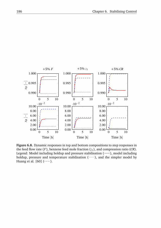
186 Chapter 6. Stabilising Control
0 5 10
0.990
0.995
1.000
x D[−
]
+5% F
0 5 10
0.990
0.995
1.000+5% z1
0 5 10
0.990
0.995
1.000+5% CR
0 5 100.002.004.006.008.00
10.00·10−2
Time [h]
x B[−
]
0 5 100.002.004.006.008.00
10.00·10−2
Time [h]
0 5 100.002.004.006.008.00
10.00·10−2
Time [h]
Figure 6.8. Dynamic responses in top and bottom compositions to step responses inthe feed flow rate (F), benzene feed mole fraction (z1), and compression ratio (CR).Legend: Model including holdup and pressure stabilisation ( ), model includingholdup, pressure and temperature stabilisation ( ), and the simpler model byHuang et al. [60] ( ).

Chapter7
Optimising Control
Optimal operation of a heat-integrated distillation column with
compressor(s) is formulated. The optimal operation is identi-
fied for a concentric heat-integrated distillation column sepa-
rating benzene/toluene. A control structure of the supervisory
control layer is devised and evaluated by simulation. The find-
ings of the case study are generalised and a control structure
of the concentric HIDiC is formulated and presented. The eco-
nomic plant-wide control method by Larsson and Skogested was
adopted for devising the control structure in a systematic man-
ner [T. Larsson and S. Skogestad. Plantwide control–a review
and a new design procedure. Model Ident Control, 21(4):209–
240, 2000]. The previously developed regulatory control layer
was combined with the supervisory control layer, and simu-
lations were carried out for evaluating the performance w.r.t.
tracking of the optimal operation.
This chapter is based on work conducted in collaboration with
Professor Sigurd Skogestad during an exchange period at the
Norwegian University of Science and Technology, Trondheim,
Norway.
A part of this chapter was is presented in the conference pro-
ceedings of DYCOPS 2016 [T. Bisgaard, S. Skogestad, J.K. Hu-
usom, and J. Abildskov. Optimal operation and stabilising con-
trol of the concentric heat-integrated distillation column. 11thIFAC International Symposium on Dynamics and Control of Pro-

188 Chapter 7. Optimising Control
cess Systems – Trondheim, Norway, 2016]. Early progress on
this problem was presented during the Nordic Process Control
Workshop 2015 (NPCW19) in Norway.

7.1. Introduction 189
7.1 Introduction
One important goal of control, after stabilisation of a plant, is ensuring optimal
operation. As will be described in the following subsection, these two tasks are
linked in the sense that the stabilising control structure must act upon the changes
performed by the optimising control structure.
7.1.1 Economic Plant-wide Control (Part 2)
In Section 6.1.2, a method for designing an economic plant-wide control structure
was described. According to the method (Figure 6.2), it is recommended to start
with the top-down design followed by the bottom-up design. However, it was found
more suitable to present the design of the control structure of the regulatory layer
(Step 5) from the bottom-up analysis (Chapter 6) prior to the top-down analysis
provided in this chapter. The top-down analysis covers Step 1-4 of the economic
plant-wide control design procedure. The argument for this is that only one unit
operation is considered, and therefore Step 5 can be performed for a given operat-
ing point. Hence, this chapter presents the application of the top-down analysis of
the economic plant-wide control method on a heat-integrated distillation column
configuration.
7.1.2 Optimising Control
The supervisory control layer is located on top of the regulatory control layer in the
control hierarchy (illustrated in Figure 6.1). The main objective of this layer is to
ensure near-optimal operation by controlling carefully selected variables, called the
primary controlled variables (CV2). The criteria for selecting the primary controlled
variables is that the economic loss must be low during disturbances, while the pri-
mary controlled variables are kept constant. The economic loss is defined as the
deviation of the actual value of the operating objective function from the optimal
value. In many cases, this implies that active constraints should be selected as pri-
mary controlled variables [104], while the remaining primary controlled variables
are selected based on the concept of self-optimising variables [149].
It was concluded, in relation to the development of the regulatory control layer,
that stabilisation of the pressure is important, and that adding a temperature con-
troller in the stabilisation layer could significantly enhance the overall stabilisation
performance. Since the pressure difference of the two column sections is essential
for the separation capability of an HIDiC, the study of the optimal operation is im-
portant. The procedure of devising the supervisory control layer and its evaluation
are presented in the following sections.

190 Chapter 7. Optimising Control
7.1.3 Case Study
The feed specifications, separation specifications, and parameter specifications of
the separation of benzene/toluene are provided in Section 6.1.5. Based on the pro-
vided design, it is desired to identify the optimal operating point. The procedure
for obtaining the optimal operating point is illustrated in Figure 7.1. In Step 1, the
conceptual design is developed of a HIDiC, which separates a given mixture of ben-
zene/toluene into 99.5% pure benzene in the distillate and 99.5% toluene in the
bottoms products. The design, satisfying these specifications, was presented previ-
ously (Section 4.5.1). In Step 2, the column internals are designed. The concentric
HIDiC is considered. The tray geometrical parameters are taken from Table 5.1 and
the total cross sectional areas of each tray were estimated as described in Section
3.4. Using this approach, the design summarised in Table 6.1 was obtained. Note,
that this approach accounts for e.g. tray pressure drop increases with increasing
vapour loading, and therefore represents a realistic HIDiC column. Based on this
column design, the identification of the optimal operating point is carried out in
Step 3. The identification of the optimal operating point is carried out as a part of
the top-down design procedure, which is described in the following sections.
1. Conceptualdesign (Chapter 4)
2. Design col-umn internals
3. Identifyoptimal operation
Figure 7.1. Case study design procedure.
7.2 Top-down Design
This analysis considers the operation aspect only. It is the purpose of this section
to define the optimal operating point based on a given column design. Hence,
an optimisation degrees of freedom analysis and the identification of the optimal
operating point will be described in this section.
7.2.1 Definition of Optimal Operation
The economic objective of operation is to maintain optimum trade-off between sep-
aration quality and operating costs associated with the compressor and reboiler.
The product prices are 1.04 $kg−1 for benzene (distillate), 0.853 $kg−1 for toluene
(bottoms) [64] and the feed price is assumed to be 0.50 $kg−1. The objective func-

7.2. Top-down Design 191
tion (J [=] $kg−1) becomes:
minJ =1
MW F F[0.50−1.04MW DD−0.853MW BB
+(
1.99+16.2(Psteam−101.3)0.05)
fsteam
+0.080 ·10−3 fcw +3.89 ·10−5E]
(7.1)
s.t.0.99≤ xD
0.99≤ 1− xB
E ≤ 550kW
101.3kPa≤ Pi ≤ 600kPa, i = 1,2, . . . ,NS
0.01F0 ≤ Li ≤ 200mols−1, i = 1,2, . . . ,NS−1
0.01F0 ≤Vi ≤ 150mols−1, i = 2,3, . . . ,NS
where
fcw = mass flow rate of cooling water [kgs−1]
fsteam = mass flow rate of steam at pressure Psteam [kgs−1]
F0 = nominal feed flow rate [mols−1]
Note that the specified product requirements in Eq. (7.1) are less strict than the
product requirements, which form the basis of the conceptual design. This reflects
a typical practice of conceptual design, where a given distillation column design
is oversized in order to improve the operation flexibility. This ensures that the re-
quired purities can be satisfied when subject to disturbances and thus increases the
flexibility of operation. Additional constraints are imposed reflecting the limita-
tions of the capacity of the equipment. These bounds are fixed by the mechanical
strength of the equipment. The upper limits of the internal flow rates were assumed
to be +50% of the nominal design values. The lower limits were assumed to be 1%
of the feed flow rate in order to avoid the possibility of certain trays drying out. A
maximum compressor duty was also assumed as +50% of the design value. The
design value refers to the values, forming the basis of the conceptual design.
The number of operational degrees of freedom was provided in Table 6.2 in
Section 6.2.1. In this context, it was argued that the considered HIDiC has eight
operational degrees of freedom, of which four have no steady state effect, and thus
no impact on the cost function in Eq. (7.1). The remaining four variables with
steady state effects are thus:
u1 = [Lcnd ,Qrbl ,Pstr,CR]T (7.2)
Note that the compression ratio (CR) is used to represent the rectifying section
pressure Prct .
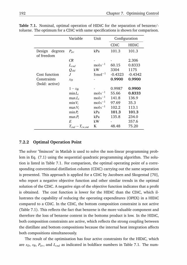
192 Chapter 7. Optimising Control
Table 7.1. Nominal, optimal operation of HIDiC for the separation of benzene/-toluene. The optimum for a CDiC with same specifications is shown for comparison.
Variable Unit Configuration
CDiC HIDiC
Design degreesof freedom
Pstr kPa 101.3 101.3
CR - - 2.306Lcnd mols−1 60.15 0.8333Qrbl kW 3304 1175
Cost function J $mol−1 -0.4323 -0.4342Constraints(bold: active)
xD - 0.9900 0.9900
1− xB - 0.9987 0.9900minLi mols−1 55.66 0.8333maxLi mols−1 141.8 136.9minVi mols−1 97.69 35.3maxVi mols−1 102.2 113.1minPi kPa 101.3 101.3maxPi kPa 135.8 234.0E kW - 357.6Tcnd−Tcw,out K 48.48 75.20
7.2.2 Optimal Operation Point
The solver "fmincon" in Matlab is used to solve the non-linear programming prob-
lem in Eq. (7.1) using the sequential quadratic programming algorithm. The solu-
tion is listed in Table 7.1. For comparison, the optimal operating point of a corre-
sponding conventional distillation column (CDiC) carrying out the same separation
is presented. This approach is applied for a CDiC by Jacobsen and Skogestad [70],
who report a negative objective function and other similar trends in the optimal
solution of the CDiC. A negative sign of the objective function indicates that a profit
is obtained. The cost function is lower for the HIDiC than the CDiC, which il-
lustrates the capability of reducing the operating expenditures (OPEX) in a HIDiC
compared to a CDiC. In the CDiC, the bottom composition constraint is not active
(Table 7.1). This reflects the fact that benzene is the more valuable component and
therefore the loss of benzene content in the bottoms product is low. In the HIDiC,
both composition constraints are active, which reflects the strong coupling between
the distillate and bottom compositions because the internal heat integration affects
both compositions simultaneously.
The result of the optimisation has four active constraints for the HIDiC, which
are xD, xB, Pstr, and Lcnd as indicated in boldface numbers in Table 7.1. The num-
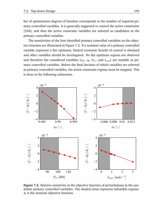
7.2. Top-down Design 193
ber of optimisation degrees of freedom corresponds to the number of required pri-
mary controlled variables. It is generally suggested to control the active constraints
[104], and thus the active constraint variables are selected as candidates as the
primary controlled variables.
The sensitivities of the four identified primary controlled variables on the objec-
tive function are illustrated in Figure 7.2. If a nominal value of a primary controlled
variable represent a flat optimum, limited economic benefit of control is obtained
and other variables should be investigated. No flat optimum regions are observed
and therefore the considered variables (xD, xB, Pstr, and Lcnd) are suitable as pri-
mary controlled variables. Before the final decision of which variables are selected
as primary controlled variables, the active constraint regions must be mapped. This
is done in the following subsection.
0.985 0.99 0.995−4
−2
0
2
4·10−4
xD [−]
(J−
J 0)/
J 0[−
]
0.006 0.008 0.01 0.012−4
−2
0
2
4·10−4
xB [−]
(J−
J 0)/
J 0[−
]
90 100 110−4
−2
0
2
4·10−4
Pstr [kPa]
(J−
J 0)/
J 0[−
]
0 1 2 3−4
−2
0
2
4·10−4
Lcnd[mols−1
]
(J−
J 0)/
J 0[−
]
Figure 7.2. Relative sensitivity in the objective function of perturbations in the can-didate primary controlled variables. The shaded areas represent infeasible regions.J0 is the nominal objective function.

194 Chapter 7. Optimising Control
7.2.3 Active Constraint Regions
The expected economic disturbances are the feed flow rate and the feed composi-
tion. The expected disturbance ranges are between -20% and +20% for the feed
composition (10% increment) and -20% and +40% for the feed flow rate (10% in-
crement). Table 7.1 only reflects the optimal operation conditions for the nominal
disturbance values. It is desired to identify the active constraints and the objec-
tive function values for every possible disturbance scenario. This identification was
carried out by the "brute force" method, which requires a discretisation of the two-
dimensional disturbance space. For this purpose, a 5×7 grid was adopted, leading
to 35 nodes. In each of the 25 nodes, the optimal solution was manually obtained
by solving Eq. (7.1) and the active constraints were recorded. When the complete
disturbance space was covered, the different active constraint regions were identi-
fied based on the obtained active constraints for the individual nodes. The resulting
map of active constraint regions is illustrated in Figure 7.3.
The active constraint Region I clearly dominates in Figure 7.3. Different con-
straints become active at relatively high feed flow rates (above +30%). At these
high feed flow rates, the maximum vapour flow rate constraint (Region II) or max-
imum compressor duty (Region III) constraint become active. The following iden-
tified active constraint regions are:
I: AC = {xD,xB,Pmin,Lmin}
II: AC = {xD,xB,Pmin,Vmax}
III: AC = {xD,xB,Pmin,Emax}
The variables refer to the bounds defined in Eq. (7.1). It is observed, that the
objective function becomes more sensitive to the feed flow rate as the feed flow
rate increases. This is because the internal heat transfer rates do not scale with
feed flow rate, as the heat exchange area is fixed. To compensate for the increased
feed flow rate, either the compressor duty must increase in order to increase the
temperature driving force (and thus the internal heat transfer rate), or the reboiler
duty must increase. However, the tray pressure drops increases with increasing
reboiler duty.
In principle, a control structure of the supervisory layer should be defined for
each active region. But for the considered concentric HIDiC, the active constraint
Region I dominates most of the disturbances encountered. As a result, only the
following primary controlled variables are considered:
CV2 = [xD,xB,Pstr,Lcnd ]T (7.3)

7.3. Supervisory Control Layer Design 195
66.7 74.95 83.2 91.45 99.7 107.95 116.2
0.6
0.55
0.5
0.45
0.4
−0.45
−0.445
−0.44−0.44
−0.435−0.435
−0.43 −0.43
−0.425 −0.425
−0.42 −0.42
I
II
III
Feed flow rate[mols−1
]
Ben
zene
mol
efr
acti
on[−
]
Figure 7.3. Active constraint regions with objective function contours [$kg−1].The active constraint regions are represented by roman numbers and they are: I:xD,xB,Pmin,Lmin; II: xD,xB,Pmin,Vmax; III: xD,xB,Pmin,Lmin,Emax; The black region rep-resents infeasibility. The subscripts "min" and "max" refers to the limits in Eq. 7.1of the corresponding varibles. Flooding is predicted in the dotted region.
In the following section, the control structure based on these primary controlled
variables will be devised.
7.3 Supervisory Control Layer Design
The design of the supervisory control layer involves several decisions, including the
pairing, the controller type, and eventual coordination between the control loops.

196 Chapter 7. Optimising Control
The simplest structure of the supervisory control layer is a decentralised scheme,
but in some cases the interactions between the loops are large, resulting in poor
dynamic performance. In such cases, the supervisory controller, or part of it, may
be multi-variable. For example, it could be a 3× 3-pairing for a model predictive
controller (MPC), which changes the setpoints of ∆T , Prct and Pstr. However, one
disadvantage of multi-variable control is the increased required computational ef-
fort.
In this work, a supervisory control layer consisting of PI controllers was selected
for the concentric HIDiC, which leads to a control structure of cascade controllers
(regulatory and supervisory control layers). In the previous analysis, it was shown
that all active constraint variables should be controlled, i.e. the top composition
(xD), the bottom composition (xB), the stripping section pressure (Pstr) and the liq-
uid reflux rate (Lcnd). These variables are primary controlled variables as they en-
sure near optimal economic performance when kept constant during disturbances.
Previously, a stabilising control structure was devised for both the case, where the
distillate product is more valuable, and the case, where the bottom product is more
valuable. Hence, the design of the supervisory control layer follows the same ap-
proach.
7.3.1 More Valuable Top Product
Generally, it is suggested to manipulate the setpoint of the temperature profile
controller (∆T set) for controlling the composition of the more valuable compo-
nent. Hence, the cascade loop employing a composition controller (CC) is used
(∆T set → xD). Using the "pair close" rule (Section 6.1.3), it is decided to control the
bottom composition (xB) by the stripping section pressure (Psetstr → xB). However, as
the stripping section pressure is also a primary controlled variable, the output from
the bottom composition controller (the stripping section pressure setpoint (Psetstr ))
must be controlled by an additional controller. This additional controller manipu-
lates the setpoint of the rectifying section in order to control the stripping section
setpoint (Psetrct → Pset
str ). The final control structure, consisting of both the regulatory
control and supervisory control layer, is illustrated in Figure 7.4(a).
7.3.2 More Valuable Bottom Product
The case where the bottom product is more valuable, the control of the temperature
profile in the stripping section is carried out by manipulating the condenser duty.
This leads to the situation where the setpoint of the temperature profile controller
(∆T set) must be manipulated by a bottom composition controller (∆T set → xB). This

7.3. Supervisory Control Layer Design 197
might appear counter-intuitive as the physical distance between the bottom product
and the condenser duty is large, which opposes the "pair close" rule. However, it is
argued that this is reasonable due to the two following reasons. The first reason is
the fact that the RGA analysis strongly favoured the pairing between the condenser
duty and the temperature profile controller in Chapter 6. The second reason is that
the actual "distance" between the bottoms product and the condenser duty is close
due to internal heat integration, i.e. the time delay is smaller than in a conven-
tional distillation column. Finally, it is proposed to control the top composition by
manipulating the rectifying section pressure setpoint (Psetrct → xD), while the optimal
value of the stripping section is passed directly through the supervisory layer to the
stripping section. The resulting control structure with both the regulatory control
and supervisory control layer for this case is illustrated in Figure 7.4(b).

198 Chapter 7. Optimising Control
LC
LC
PCQ
cnd
D
E
Mcnd
ΔT MrctPrct
Pstr Qrbl
B
LC
LC
PC
LC
Qcnd
D
Lint
E
Mcnd
Mrct
Mrct
Pstr Qrbl
B
PC
Pstropt
Prctset
FC
Lcnd
Lcnd
Lcndopt
CC
x Dopt
x D
ΔTset C
Cx B
Pstrset
x Bopt
TD
C
LC
LC
PC
PC
LC
Qcnd
D
Lint
E
Mcnd
Mrct
ΔT
Mrct
Prct
Pstr Qrbl
B
Prctset
FC
Lcnd
Lcnd
Lcndopt
CC
x Dopt
x D
PC
x B
x Bopt
ΔTset
Reg
ula
tory
Top
val
uab
le (
wit
h
2xC
A)
Bo
tto
m v
alu
able
Pstropt
PC
DT
C
Prct
ΔT
DT
C
LC
Lint
Mint
PC
FC
Lcnd
LC
LC
PCQ
cnd
D
E
Mcnd
ΔT
MrctPrct
Pstr Qrbl
B
PC
DT
C
LC
Lint
MintFC
Lcnd
LC
LC
PCQ
cnd
D
E
Mcnd
ΔT MrctPrct
Pstr Qrbl
B
PC
DT
C
LC
Lint
Mint
FC
Lcnd
Lcndopt
CC
x BPstrset x Bopt
PC
Pstropt
CC
x Dopt
x D
Prctset
Pstrset
LC
LC
PCQ
cnd
D
E
Mcnd
ΔT
MrctPrct
Pstr Qrbl
B
PC
DT
C
LC
Lint
Mint
FC
Lcnd
Lcndopt
x Bx Bopt
CC
ΔTset
ΔTset
x Dopt
x D
CC
Prctset
Pstropt
(a)
Dis
tilla
tem
ore
valu
able
prod
uct.L
C
LC
PCQ
cnd
D
E
Mcnd
ΔT MrctPrct
Pstr Qrbl
B
LC
LC
PC
LC
Qcnd
D
Lint
E
Mcnd
Mrct
Mrct
Pstr Qrbl
B
PC
Pstropt
Prctset
FC
Lcnd
Lcnd
Lcndopt
CC
x Dopt
x D
ΔTset C
Cx B
Pstrset
x Bopt
TD
C
LC
LC
PC
PC
LC
Qcnd
D
Lint
E
Mcnd
Mrct
ΔT
Mrct
Prct
Pstr Qrbl
B
Prctset
FC
Lcnd
Lcnd
Lcndopt
CC
x Dopt
x D
PC
x B
x Bopt
ΔTset
Reg
ula
tory
Top
val
uab
le (
wit
h
2xC
A)
Bo
tto
m v
alu
able
Pstropt
PC
DT
C
Prct
ΔT
DT
C
LC
Lint
Mint
PC
FC
Lcnd
LC
LC
PCQ
cnd
D
E
Mcnd
ΔT
MrctPrct
Pstr Qrbl
B
PC
DT
C
LC
Lint
MintFC
Lcnd
LC
LC
PCQ
cnd
D
E
Mcnd
ΔT MrctPrct
Pstr Qrbl
B
PC
DT
C
LC
Lint
Mint
FC
Lcnd
Lcndopt
CC
x BPstrset x Bopt
PC
Pstropt
CC
x Dopt
x D
Prctset
Pstrset
LC
LC
PCQ
cnd
D
E
Mcnd
ΔT
MrctPrct
Pstr Qrbl
B
PC
DT
C
LC
Lint
Mint
FC
Lcnd
Lcndopt
x Bx Bopt
CC
ΔTset
ΔTset
x Dopt
x D
CC
Prctset
Pstropt
(b)
Bot
tom
sm
ore
valu
able
prod
uct.
Figu
re7.
4.C
ontr
olst
ruct
ures
for
aH
IDiC
.R
edlin
esre
pres
ent
the
regu
lato
ryco
ntro
llo
ops
and
blue
lines
repr
esen
tsu
perv
isor
yco
ntro
llo
ops
(cas
cade
).LC
:Le
vel
cont
rolle
r,PC
:Pr
essu
reco
ntro
ller,
DTC
:D
iffe
renc
ete
mpe
ratu
reco
ntro
ller,
FC:
Flow
cont
rolle
r,C
C:c
ompo
siti
onco
ntro
ller.

7.4. Dynamic Evaluation 199
7.4 Dynamic Evaluation
In this section, the developed supervisory layer control structure, combined with
the regulatory layer, is evaluated by dynamic simulation. The distillate is the more
valuable product for the separation of benzene/toluene and thus the final control
structure of Figure 7.4(a) is employed.
7.4.1 Tuning
A sequential tuning was carried out in the order displayed in Table 7.2. The table
includes the identified first-order models, the desired closed-loop time constants,
and the resulting controller parameters. Since the controllers of the supervisory
layer act as cascade controllers, desired closed-loop time constants ten times larger
than those of the slave loops from the regulatory control layer were used.
7.4.2 Evaluation
The developed control structure consisting of a regulatory and a supervisory layer
is evaluated for the different disturbance scenarios, given below.
7.4.2.1 Single Disturbance Scenarios
The following disturbance scenarios are used to investigate the performance of the
control layers. The dynamic responses for feed flow rate step changes are illustrated
in Figure 7.5, given the scenario:
• 0 < t ≤ 15h: +10% feed flow rate
• 15h < t: Feed flow rate reset (F = F0)
The dynamic responses for feed composition step changes are illustrated in Figure
7.6, given the scenario:
• 0 < t ≤ 15h: +10% feed composition
• 15h < t: Feed composition reset (z = z0)
Both the disturbance scenarios lead to a new steady state after approximately 15 h.
The primary controlled variables (CV1) are shown in the left columns of Figure
7.5 and Figure 7.6. These (CV1) are controlled by the supervisory control layer by
adjusting the setpoints of CV2, which are illustrated in the middle columns. The
CV2 are controlled by the regulatory control layer by adjusting the actuators uD
in the columns to the right. Both disturbance scenarios are controlled reasonably

200 Chapter 7. Optimising Control
Table 7.2. Sequential tuning (ordered) of the concentric HIDiC with dynamic re-sponses. In each row, the above control loops are closed. The unit of the pressuresis bar. Legend: Dynamic responses ( ), fitted transfer functions, G(s) ( ).
Loop Response Controller parameters
∆y vs. t/τc G(s) τc Kc τIs s
∆T set → xD
0 2 4
−4
−2
0·10−3
−5.074·10−3
439.4s+1 e−293.8s 1200 -57.97 439.4
Psetstr → xB
0 2 405
1015
·10−20.1809
789.4s+1 e−401.3s 1200 2.726 789.4
Psetrct → Pset
str
0 2 40
0.2
0.4
0.60.5523
1371s+1 e−267.8s 12,000 0.2023 1.371
well. As expected, the distillate compositions are more tightly controlled than the
bottoms compositions because the temperature controller is located in the rectifying
section.

7.4. Dynamic Evaluation 201
1
010
2030
0.97
0.98
0.99
1.00
xD[−]
CV
1
010
2030
7.88
8.2
8.4
∆T[K]
CV
2
010
2030
−1,
400
−1,
300
−1,
200
Qcnd[kW]
u D
010
2030
0.00
1.00
2.00
3.00·1
0−2
xB[−]
010
2030
9698100
102
104
Pstr[kPa]
010
2030
1,15
0
1,20
01,
250
1,30
0
Qrbl[kW]
010
2030
9698100
102
104
Tim
e[h]
Pstr[kPa]
010
2030
210
215
220
225
230
Tim
e[h]
Prct[kPa]
010
2030
360
380
400
420
Tim
e[h]
E[kW]
Figu
re7.
5.D
ynam
icre
spon
ses
inco
ntro
lled
and
man
ipul
ated
vari
able
sto
step
chan
ges
inth
efe
edflo
wra
te.
Lege
nd:
All
loop
scl
osed
(),
setp
oint
().

202 Chapter 7. Optimising Control
1
010
2030
0.97
0.98
0.99
1.00
xD[−]C
V1
010
2030
7.4
7.6
7.88
8.2
∆T[K]
CV
2
010
2030
−1,
400
−1,
300
−1,
200
Qcnd[kW]
u D
010
2030
0.00
1.00
2.00
3.00·1
0−2
xB[−]
010
2030
95100
105
Pstr[kPa]0
1020
30
1,20
0
1,40
0
Qrbl[kW]
010
2030
95100
105
Tim
e[h]
Pstr[kPa]
010
2030
205
210
215
220
Tim
e[h]
Prct[kPa]
010
2030
320
340
360
380
Tim
e[h]
E[kW]
Figu
re7.
6.D
ynam
icre
spon
ses
inco
ntro
lled
and
man
ipul
ated
vari
able
sto
step
chan
ges
inth
efe
edco
mpo
siti
on.
Lege
nd:
All
loop
scl
osed
(),
setp
oint
().
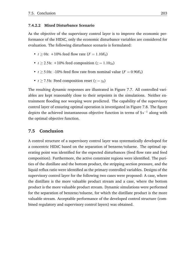
7.5. Conclusion 203
7.4.2.2 Mixed Disturbance Scenario
As the objective of the supervisory control layer is to improve the economic per-
formance of the HIDiC, only the economic disturbance variables are considered for
evaluation. The following disturbance scenario is formulated:
• t ≥ 0h: +10% feed flow rate (F = 1.10F0)
• t ≥ 2.5h: +10% feed composition (z = 1.10z0)
• t ≥ 5.0h: -10% feed flow rate from nominal value (F = 0.90F0)
• t ≥ 7.5h: Feed composition reset (z = z0)
The resulting dynamic responses are illustrated in Figure 7.7. All controlled vari-
ables are kept reasonably close to their setpoints in the simulations. Neither en-
trainment flooding nor weeping were predicted. The capability of the supervisory
control layer of ensuring optimal operation is investigated in Figure 7.8. The figure
depicts the achieved instantaneous objective function in terms of $s−1 along with
the optimal objective function.
7.5 Conclusion
A control structure of a supervisory control layer was systematically developed for
a concentric HIDiC based on the separation of benzene/toluene. The optimal op-
erating point was identified for the expected disturbances (feed flow rate and feed
composition). Furthermore, the active constraint regions were identified. The puri-
ties of the distillate and the bottom product, the stripping section pressure, and the
liquid reflux ratio were identified as the primary controlled variables. Designs of the
supervisory control layer for the following two cases were proposed: A case, where
the distillate is the more valuable product stream and a case, where the bottom
product is the more valuable product stream. Dynamic simulations were performed
for the separation of benzene/toluene, for which the distillate product is the more
valuable stream. Acceptable performance of the developed control structure (com-
bined regulatory and supervisory control layers) was obtained.
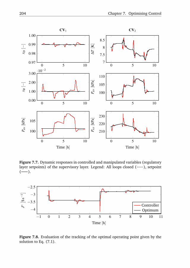
204 Chapter 7. Optimising Control1
0 5 100.97
0.98
0.99
1.00
x D[−
]
CV1
0 5 107
7.5
8
8.5
∆T[K]
CV2
0 5 100.00
1.00
2.00
3.00·10−2
x B[−
]
0 5 10
100
105
110
P str[k
Pa]
0 5 10
100
105
Time [h]
P str[k
Pa]
0 5 10
210
220
230
Time [h]
P rct[k
Pa]
Figure 7.7. Dynamic responses in controlled and manipulated variables (regulatorylayer setpoints) of the supervisory layer. Legend: All loops closed ( ), setpoint( ).
−1 0 1 2 3 4 5 6 7 8 9 10 11
−4
−3.5
−3
−2.5
Time [h]
J∗[ $
s−1]
ControllerOptimum
Figure 7.8. Evaluation of the tracking of the optimal operating point given by thesolution to Eq. (7.1).

Chapter8
Thesis Conclusions
Introducing heat-integration in distillation by the means of compression results
in a trade-off between operating expenditures (OPEX) and capital expenditures
(CAPEX). The heat-integrated distillation column (HIDiC) offers a low OPEX but
a high CAPEX, relative to conventional distillation. The high CAPEX relates to the
investment costs of the compressor and the internal heat exchangers. The me-
chanical vapour recompression column also offers lower OPEX and higher CAPEX
than conventional distillation. It was found that the HIDiC offers the lowest OPEX
among the considered distillation column configurations for binary separations with
a normal boiling point difference below 10 K. For binary separations with a normal
boiling point difference above 10 K, the secondary reflux and vaporisation column
(SRVC) has the lowest OPEX. It is expected that these findings will facilitate a fo-
cused development of cheap and simple heat panels in order to reduce the CAPEX
of internal heat exchangers.
A systematic modelling and conceptual design framework was developed, which
is tailor-made for the four considered configurations: The MVRC, the HIDiC, the
SRVC, and the conventional distillation column. The framework allows static and
dynamic benchmarking of all configurations. The model accounts for vital phenom-
ena such as pressure dynamics, liquid tray hydraulics, and sensible heat effects.
Due to the general structure of the model, a possibility exists for incorporating ad-
ditional heat-integrated distillation column configurations with one or more com-
pressors. Another benefit of the general model formulation is that it allows a fair
basis for comparison when conducting configuration benchmark studies. All model
equations for the individual configurations are solved within the same framework,
and therefore the same economic model, the same model parameters, etc.
In order to study a realistic operation of a concentric HIDiC, a regulatory control
layer and a supervisory control layer were devised and evaluated by simulation. The
206 Chapter 8. Thesis Conclusions
control structure designs were based on general consideration and a numerical case
study of the separation of benzene/toluene. Hence, recommendations are given on
the control structures of both control layers.
This work has addressed two main areas in the development and understanding
of using compressors in heat-integrated distillation. The first area is the economic
feasibility, which was described above. The second area is the technical feasibility.
The study of the separation of benzene/toluene has been adopted to show that:
• The specified uniform heat integration area by design can be realised within
the HIDiC.
• Additional utility should be considered; the vapour inlet to the compressor
must be superheated in order to avoid condensation within the compressor.
• Neither entrainment flooding nor weeping were encountered in three column
arrangements: A HIDiC with uniform column area, a concentric HIDiC with
gradually changing rectifying section area, and a simplified concentric HIDiC,
in which the rectifying section area is gradually decreased over three parti-
tions.
• The HIDiC can be operated steadily using a proposed, decentralised regula-
tory control layer. Steady operation means in this context that the drifting
variables were maintained at their setpoints and that no entrainment flood-
ing or weeping were observed during dynamic simulations. This conclusion
is based on the concentric HIDiC.
• The HIDiC can be operated steadily and with good tracking of an economic
objective function using a decentralised, supervisory control layer on top of
the regulatory control layer. This conclusion is based on the concentric HIDiC.

Chapter9
Future Directions
The main concern of the development of the heat-integrated distillation column
(HIDiC) is the understanding of the realisation of internal heat-integration on an
industrial scale. Among the proposed column arrangements for addressing this,
are the shell-and-tube arrangement, the concentric arrangement, and the struc-
tured plate arrangement. Based on the findings in this work and in literature, some
drawbacks of the mentioned arrangements are:
• The shell-and-tube arrangement has negative effects on the separation.
• The concentric arrangement can only accommodate the required heat ex-
change area by installing heat panels within the structure.
• The shell-and-tube arrangement and the structured plate arrangement only
exist as packed columns.
• The realisation of internal heat integration is constrained by the construction
cost.
It has been found that the construction cost of internal heat exchangers is the main
economic bottleneck. One option is to reduce the number of internal heat exchang-
ers, while another option is to improve the design of the internal heat exchangers.
Computational fluid dynamics (CFD) is a powerful simulation tool, which can be
employed to develop, innovate, and optimise the column arrangement for real-
ising internal heat transfer. Using CFD, the implications w.r.t. heat transfer and
mass transfer of realising internal heat integration in distillation can be quanti-
fied. Based on these quantifications, the heat and mass transfer phenomenons can
be fully understood and appropriate measures can be taken in order to improve
designs. In addition, economic construction constraints can be investigated by sim-
ulation, thereby reducing possible costs associated with experimental testing. In
208 Chapter 9. Future Directions
relation to the experimental observation, the concentric arrangement with trays
and heat panels, and the structured plate arrangements, appear to be good candi-
dates for industrial-scale HIDiC applications. Furthermore, determinations of the
overall heat transfer coefficients inside various internal heat-integrated distillation
column arrangements are well documented in literature.
The developed model is only designed for performing dynamic simulations of
ideal vapour systems. The propylene/propane distillation column was found to be
a feasible economic alternative to the mechanical vapour recompression column
(MVRC). Furthermore, it was found that pressure dynamics were essential in the
study of the operation of the HIDiC. Because the propylene/propane distillation
column has almost two hundreds trays, pressure propagations within the column
are significant for the operation. Thus, it is essential to study the operation of a
HIDiC carrying out such a separation. The developed model must be extended to
cover such separations, i.e. a differential-algebraic equation (DAE) system must be
formulated and solved.
Automatising the proposed design method has not been completed in this study.
If such automation is successful, a possibility for conducting extensive combina-
torial studies arises, in order to arrive at a true optimal structure. This approach
will then be an alternative to the super structure-based approach of Harward and
Marquardt [51].
Bibliography
[1] Economic indicators. Technical report, Chemical Engineering, 2012.
[2] Danske nøgletal. http://www.ens.dk/info/tal-kort/
statistik-nogletal/nogletal/danske-nogletal, 2015. December,
2015.
[3] U.S. Energy Information Adminstration. Petroleum and other liquids. www.
eia.gov, 2015. January, 2016.
[4] William H. Aitken. Apparatus for combined heat and mass transfer, 1998.
US Patent 5,722,258.
[5] J.R. Alcántara-Avila and H.-Y. Lee. Process Intensification in Chemical Engi-neering. Design Optimization and Control, chapter 5 Heat-Integrated Inten-
sified Distillation Processes. J.G. Segovia-Hernández, A. Bonilla-Petriciolet,
1st edition. edition, 2016.
[6] T.R. Andersen. Optimal Design and Operation of Process Integrated Distilla-tion. PhD thesis, Technical University of Denmark, 2002.
[7] K. Aso, H. Matsuo, H. Noda, T. Takada, and N. Kobayashi. Heat integrated
distillation operation, 1998. US Patent 5,783,047.
[8] F.E. Becker and A.I. Zakak. Heat recovery in distillation by mechanical vapor
recompression. Proceedings from the Eighth Annual Industrial Energy Technol-ogy Conference, pages 705–709, 1986.
[9] L.T. Biegler, I.E. Grossmann, and A.W. Westerberg. Systematic Methods ofChemical Process Design. Prentice-Hall Inc., New Jersey. USA, 1st edition.
edition, 1997.
[10] T. Bisgaard, J.K. Huusom, and J. Abildskov. Dynamic effects of diabatiza-
tion in distillation columns. Proceedings of the 10th European Workshop on

210 Bibliography
Advanced Control and Diagnostics (ACD 2012), 2012.
[11] T. Bisgaard, J.K. Huusom, and J. Abildskov. Dynamic effects of diabatiza-
tion in distillation columns. Computer-aided Chemical Engineering, 32:1015–
1020, 2013.
[12] T. Bisgaard, J.K. Huusom, and J. Abildskov. A modeling framework for con-
ventional and heat integrated distillation columns. 10th IFAC InternationalSymposium on Dynamics and Control of Process Systems – Mumbai, India,
pages 373–378, 2013.
[13] T. Bisgaard, J.K. Huusom, and J. Abildskov. Impact on model uncertainty of
diabatization in distillation columns. Proceedings of Distillation and Absorp-tion, pages 909–914, 2014.
[14] T. Bisgaard, J.K. Huusom, and J. Abildskov. Modeling and analysis of
conventional and heat-integrated distillation columns. AIChE Journal,61(12):4251–4263, 2015.
[15] T. Bisgaard, J.K. Huusom, and J. Abildskov. Conceptual design of heat-
integrated distillation columns with compressors. 2016.
[16] T. Bisgaard, S. Skogestad, J.K. Huusom, and J. Abildskov. Optimal operation
and stabilising control of the concentric heat-integrated distillation column.
11th IFAC International Symposium on Dynamics and Control of Process Sys-tems – Trondheim, Norway, 2016.
[17] E.H. Bristol. On a new measure of interaction for multivariable process con-
trol. IEEE Transactions on Automatic Control, 11(1):133–134, 1966.
[18] A.J. Brugma. Fractional distillation of liquid mixtures, especially petroleum,
1937. US Patent 2,471,134.
[19] O.S.L. Bruinsma, T. Krikken, J. Cot, M. Saric, S.A. Tromp, Ž. Olujic, and A.I.
Stankiewicz. The structured heat integrated distillation column. Chem EngRes Des, 90(4):458–470, 2012.
[20] J. Cabrera-Ruiz, A. Jiménez-Gutiérrez, and J.G. Segovia-Hernández. Assess-
ment of the implementation of heat-integrated distillation columns for the
separation of ternary mixtures. Ind Eng Chem Res, 50(4):2176–2181, 2011.
[21] I.T. Cameron, C.A. Ruiz, and R. Gani. A generalized model for distilla-
tion columns–ii: Numerical and computational aspects. Comput Chem Eng,
10(3):199–211, 1986.
[22] J.C. Campbell, K.R. Wigal, V. Van Brunt, and R.S. Kline. Comparison of
energy usage for the vacuum separation of acetic acid/acetic anhydride using

Bibliography 211
an internally heat integrated distillation column (hidic). Separ Sci Technol,43(9–10):2269–2297, 2008.
[23] H. Chen, K. Huang, and S. Wang. A novel simplified configuration for an
ideal heat-integrated distillation column (ideal hidic). Sep Purif Technol,73(2):230–242, 2010.
[24] J. de Graauw, M.J. Steenbakker, A. de Rijke, Z. Olujic, and P.J. Jansens. Heat
integrated distillation column, 2010. US Patent 7,678,237.
[25] G. de Koeijer and R. Rivero. Entropy production and exergy loss in experi-
mental distillation columns. Chem Eng Sci, 58(8):1587–1597, 2003.
[26] G.M. de Koeijer and S. Kjelstrup. Minimizing entropy production rate in
binary tray distillation. Int J Thermodyn, 3(3):105–110, 2000.
[27] A. de Rijke. Development of a Concentric Internally Heat Integrated DistillationColumn (HIDiC). PhD thesis, Technische Universiteit Delft, 2007.
[28] A. de Rijke, W. Tesselaar, M.A. Gadalla, Z. Olujic, and P.J. Jansens. Heat and
mass transfer characteristics of an annular sieve tray. IChemE SymposiumSeries No. 152, pages 181–189, 2006.
[29] M.F. Doherty and J.D. Perkins. On the dynamics of distillation processes–
iv uniqueness and stability of the steady state in homogeneous continuous
distillations. Chem Eng Sci, 37(3):381–392, 1982.
[30] J.A. Ferré, F. Castells, and J. Flores. Optimization of a distillation column
with a direct vapor recompression heat pump. Industrial and EngineeringChemistry Process Design and Development, 24(1):128–132, 1985.
[31] R.E. Fitzmorris and R.S.H. Mah. Improving distillation column design using
thermodynamic availability analysis. AIChE J, 26(2):265–273, 1980.
[32] Z. Fonyo and P. Mizsey. Economic applications of heat pumps in integrated
distillation systems. Heat Recovery Syst CHP, 14(3):249–263, 1994.
[33] Aa. Fredenslund, J. Gmehling, and P. Rasmussen. Vapor-liquid EquilibriumUsing UNIFAC. A Contribution Method. Elsevier, USA, 1st edition. edition,
1977.
[34] D.C. Freshwater. Thermal economy in distillation. Institution of ChemicalEngineers – Transactions, 29(1):149–160, 1951.
[35] C. Fuentes and W.L. Luyben. Control of high-purity distillation columns.
Industrial and Engineering Chemistry Process Design and Development,22(3):361–366, 1983.

212 Bibliography
[36] T. Fukushima, M. Kano, O. Tonomura, and S. Hasebe. Dynamics and control
of heat integrated distillation column (hidic). International Symposium onAdvanced Control of Chemical Processes, pages 629–634, 2006.
[37] M. Gadalla, L. Jiménez, Z. Olujic, and P.J. Jansens. A thermo-hydraulic
approach to conceptual design of an internally heat-integrated distillation
column (i-hidic). Comput Chem Eng, 31(10):1346–1354, 2007.
[38] M. Gadalla, Z. Olujic, A. de Rijke, and P.J. Jansens. A thermo-hydraulic ap-
proach to conceptual design of an internally heat-integrated distillation col-
umn (i-hidic). European Symposium on Computer-Aided Process Engineering,
18:181–186, 2004.
[39] M. Gadalla, Z. Olujic, A. de Rijke, and P.J. Jansens. A new approach to
the design of internally heat-integrated tray distillation columns. EuropeanSymposium on Computer-Aided Process Engineering, 20:805–810, 2005.
[40] M. Gadalla, Z. Olujic, L. Sun, A. de Rijke, and P.J. Jansens. Pinch analysis-
based approach to conceptual design of internally heat-integrated distillation
columns. Chem Eng Res Des, 83(8):987–993, 2005.
[41] M.A. Gadalla. Internal heat integrated distillation columns (ihidics)-new
systematic design methodology. Chem Eng Res Des, 87(12A):1658–1666,
2009.
[42] R. Gani, C.A. Ruiz, and I.T. Cameron. A generalized model for distilla-
tion columns–i: Model description and applications. Comput Chem Eng,
10(3):181–198, 1986.
[43] P. Le Goff, T. Cachot, and R. Rivero. Exergy analysis of distillation processes.
Chem Eng Technol, 19(6):478–485, 1996.
[44] S. Gopichand, T.O. Omideyi, J. Kasprzycki, and S. Devotta. The economics
of heat pump assisted distillation systems–ii. analysis of ethanol-water mix-
tures. J Heat Recov Syst, 4(4):271–280, 1984.
[45] R. Govind. Dual distillation column, 1987. US Patent 4,681,661.
[46] F. Gross, E. Baumann, A. Geser, D.W.T. Rippin, and L. Lang. Modelling, simu-
lation and controllability analysis of an industrial heat-integrated distillation
process. Comput Chem Eng, 22(1–2):223–237, 1998.
[47] R. Gutiérrez-Guerra, J. Cortez-González, R. Murrieta-Dueñas, J.G. Segovia-
Hernández, S. Hernández, and A. Hernández-Aguirre. Design and optimiza-
tion of heat-integrated distillation column schemes through a new robust
methodology coupled with a boltzmann-based estimation of distribution al-

Bibliography 213
gorithm. Ind Eng Chem Res, 53(27):11061–11073, 2014.
[48] R. Gutiérrez-Guerra, R. Murrieta-Dueñas, J. Cortez-González, J.G. Segovia-
Hernández, S. Hernández, and A. Hernández-Aguirre. Design and optimiza-
tion of hidic distillation columns using a boltzmann-based estimation of dis-
tribution algorithm: Influence of volatility. Proceedings of Distillation andAbsorption, pages 655–660, 2014.
[49] D. Hänggi and I. Meszaros. Vapor recompression: Distillation without steam.
Sulzer Technical Review 1/99, pages 32–34, 1999.
[50] A. Harwardt, K. Kraemer, and W. Marquardt. Identifying optimal mixture
properties for hidic application. Proceedings of Distillation and Absorption,
pages 55–60, 2010.
[51] A. Harwardt and W. Marquardt. Heat-integrated distillation columns: Vapor
recompression or internal heat integration? AIChE J, 58(12):3740–3750,
2012.
[52] G.G. Haselden. Distillation process and apparatus, 1977. US Patent
4,025,398.
[53] J.C. Helton and F.J. Davis. Latin hypercube sampling and the propagation of
uncertainty in analyses of complex systems. Reliab Eng Syst Safe, 81(1):23–
69, 2003.
[54] E.J. Henley and J.D. Seader. Equilibrium-Stage Separation Operations inChemical Engineering. John Wiley & Sons, Inc, USA, 1st edition. edition,
1981.
[55] T. Ho, C. Huang, J. Lin, and L. Lee. Dynamic simulation for internally heat-
integrated distillation columns (hidic) for propylene-propane system. Com-put Chem Eng, 33(6):1187–1201, 2009.
[56] T.-J. Ho, C.T. Huang, L.-S. Lee, and C.-T. Chen. Extended ponchon-savarit
method for graphically analyzing and designing internally heat-integrated
distillation columns. Ind Eng Chem Res, 49(1):305–358, 2010.
[57] C.D. Holland. Fundamentals of Multicomponent Distillation. McGraw-Hill
Book, Inc., USA, 1st edition. edition, 1981.
[58] K. Horiuchi, K. Yanagimoto, K. Kataoka, and M. Nakaiwa. Energy-saving
characteristics of heat integrated distillation column technology applied to
multi-component petroleum distillation. IChemE Symposium Series No. 152,
pages 172–180, 2006.
[59] K. Huang, W. Liu, J. Ma, and S. Wang. Externally heat-integrated double

214 Bibliography
distillation column (ehiddic): Basic concept and general characteristics. IndEng Chem Res, 49(3):1333–1350, 2010.
[60] K. Huang, M. Nakaiwa, T. Akiya, K. Aso, and T. Takamatsu. A numerical
consideration on dynamic modeling and control of ideal heat integrated dis-
tillation columns. J Chem Eng Jpn, 29(2):344–351, 1996.
[61] K. Huang, L. Shan, Q. Zhu, and J. Qian. Design and control of an ideal heat-
integrated distillation column (ideal hidic) system separating a close-boiling
ternary mixture. Energy, 32(11):2148–2156, 2007.
[62] K. Huang, L. Shan, Q. Zhu, and J. Qian. Adding rectifying/stripping section
type heat integration to a pressure-swing distillation (psd) process. ApplTherm Eng, 28(8–9):923–932, 2008.
[63] K. Huang, S. Wang, K. Iwakabe, L. Shan, and Q. Zhu. Temperature con-
trol of an ideal heat-integrated distillation column (hidic). Chem Eng Sci,62(22):6486–6491, 2007.
[64] ICIS. www.icis.com, 2015. August, 2015.
[65] International Energy Agency. Energy technology perspectives 2012. Techni-
cal report, International Energy Agency, 2012.
[66] K. Iwakabe, M. Nakaiwa, K. Huang, K. Matsuda, T. Nakanishi, T. Ohmori,
A. Endo, and T. Yamamoto. An internally heat-integrated distillation column
(hidic) in japan. IChemE Symposium Series No. 152, pages 900–911, 2006.
[67] K. Iwakabe, M. Nakaiwa, K. Huang, T. Nakanishi, A. Røsjorde, T. Ohmori,
A. Endo, and T. Yamamoto. Energy saving in multicomponent separation
using an internally heat-integrated distillation column (hidic). Appl ThermEng, 26(13):1362–1368, 2006.
[68] K. Iwakabe, M. Nakaiwa, K. Huang, T. Nakanishi, A. Røsjorde, T. Ohmori,
A. Endo, and T. Yamamoto. Performance of an internally heat-integrated
distillation column (hidic) in separation of ternary mixtures. J Chem EngJpn, 39(4):417–425, 2006.
[69] E.W. Jacobsen and S. Skogestad. Multiple steady states in ideal two-product
distillation. AIChE J, 37(4):499–511, 1991.
[70] M.G. Jacobsen and S. Skogestad. Active constraint regions for optimal oper-
ation of distillation columns. Ind Eng Chem Res, 51(7):2963–2973, 2012.
[71] F. Jaing, J. Quan, T. Hamaguchi, Y. Ota, and Y. Hashimoto. Design and
control of hidic. SICE-ICASE International Joint Conference, Bexco, Busan,Korea, pages 5727–5730, 2006.
Bibliography 215
[72] C.A. Jaksland, R. Gani, and K.M. Lien. Separation process design and synthe-
sis based on thermodynamic insights. Chem Eng Sci, 50(3):511–530, 1995.
[73] A.K. Jana. Heat integrated distillation operation. Appl Energ, 87(5):1477–
1494, 2010.
[74] A.K. Jana. Advances in heat pump assisted distillation column: A review.
Energy Convers Manage, 77:287–297, 2014.
[75] E. Jensen. Rectification apparatus using a heat pump, 2011. US Patent
7,972,423.
[76] W. Jiang, J. Khan, and R.A. Dougal. Dynamic centrifugal compressor model
for system simulation. J Power Sources, 158(2):1333–1343, 2006.
[77] E.S. Jimenez, P. Salamon, R. Rivero, C. Rendon, K.H. Hoffmann, M. Schaller,
and B. Andersen. Optimization of a diabatic distillation column with sequen-
tial heat exchangers. Ind Eng Chem Res, 43(23):7566–7571, 2004.
[78] S.S. Jogwar and P. Daoutidis. Dynamics and control of vapor recompression
distillation. J of Process Contr, 19(10):1737–1750, 2009.
[79] M. Kano, T. Fukushima, H. Makita, and S. Hasebe. Multiple steady-states in
a heat integrated distillation column (hidic). J Chem Eng Jpn, 40(10):824–
831, 2007.
[80] M. Kano, H. Makita, and S. Hasebe. Prediction of multiple steady states in
distillation through simple mass and heat balance analysis. Ind Eng ChemRes, 50(3):1346–1351, 2011.
[81] K. Kataoka, H. Noda, T. Mukaida, G. Nishimura, and H. Yamaji. Boost to
bioethanol distillation by internal heat-integrated distillation column (hidic).
Advanced Chemical Engineering Reasearch, 3, 2014.
[82] Y.H. Kim. Internally and partially heat-integrated distillation system for
ternary separation. Ind Eng Chem Res, 50(9):5733–5738, 2011.
[83] B. Kiran and A.K. Jana. Introducing vapor recompression mechanism in heat-
integrated distillation column: Impact of internal energy driven intermediate
and bottom reboiler. AIChE J, 61(1):118–131, 2015.
[84] B. Kiran, A.K. Jana, and A.N. Samanta. A novel intensified heat integration
in multicomponent distillation. Energy, 41(1):443–453, 2012.
[85] A.A. Kiss. Distillation technology-still young and full of breakthrough oppor-
tunities. J Chem Technol Biotechnol, 89(4):479–498, 2013.
[86] A.A. Kiss, S.J. Flores Landaeta, and C.A. Infante Ferreira. Towards energy ef-
216 Bibliography
ficient distillation technologies - making the right choice. Energy, 47(1):531–
542, 2012.
[87] A.A. Kiss and Ž. Olujic. A review on process intensification in internally heat-
integrated distillation columns. Chem Eng and Process: Process Intensification,
86:125–144, 2014.
[88] Jr.P.A. Kolodzie and M. van Winkle. Discharge coefficienfts through perfo-
rated plates. AIChE J, 3(3):305–312, 1957.
[89] T. Larsson and S. Skogestad. Plantwide control–a review and a new design
procedure. Model Ident Control, 21(4):209–240, 2000.
[90] H. Li. Modelling for Predictive Control. PhD thesis, Technical University of
Denmark, 2007.
[91] X. Liu, M.A. Longhua, and Q. Jixin. Thermodynamic analysis and optimiza-
tion on energy savings of ideal internal thermally coupled distillation col-
umn. Chinese J Chem Eng, 8(1):57–63, 2000.
[92] X. Liu and J. Qian. Modeling, control, and optimization of ideal internal
thermally coupled distillation columns. Chem Eng Technol, 23(3):235–241,
2000.
[93] X. Liu, Y. Zhou, L. Cong, and F. Ding. High-purity control of internal ther-
mally coupled distillation columns based on nonlinear wave model. J ofProcess Contr, 21(6):920–926, 2011.
[94] R.S.H. Mah, Jr.J.J. Nicholas, and R.B. Wodnik. Distillation with secondary
reflux and vaporization: A comparative evaluation. AIChE J, 23(5):651–658,
1977.
[95] D. Maiti, A.K. Jana, and A.N. Samanta. A novel heat integrated batch distil-
lation scheme. Appl Energ, 88(12):5221–5225, 2011.
[96] H. Makita, T. Fukushima, M. Kano, and S. Hasebw. Analysis of multiple
steady-states in a heat integrated distillation column (hidic). PSE ASIA, 2007.
[97] S.V. Mali and A.K. Jana. A partially heat integrated reactive distillation:
Feasibility and analysis. Sep Purif Technol, 70(1):136–139, 2009.
[98] A. Mane. A new intensified heat integration in distillation column. Ind EngChem Res, 49(19):9534–9541, 2010.
[99] K. Matsuda, K. Iwakabe, K. Kubo, A. Horiguchi, Y. Weifang, H. Kosuge,
S. Kataoka, T. Yamamoto, T. Ohmori, and M. Nakaiwa. Rate-based modeling
for internally heat-integrated distillation column (hidic) in binary system. JJpn Pet Inst, 50(3):162–168, 2007.

Bibliography 217
[100] K. Matsuda, K. Iwakabe, and M. Nakaiwa. Recent advances in internally
heat-integrated distillation columns (hidic) for sustainable development. JChem Eng Jpn, 45(6):363–372, 2012.
[101] M. Mauricio-Iglesias, T. Bisgaard, H. Kristensen, K.V. Gernaey, J. Abildskov,
and J.K. Huusom. Pressure control in distillation columns: A model-based
analysis. Ind Eng Chem Res, 53(38):14776–14787, 2014.
[102] N. Metropolis and S. Ulam. The monte carlo method. J Am Stat Assoc,44(247):335–341, 1949.
[103] K. Meyer, L. Ianniciello, J.E. Nielsen, T. Bisgaard, J.K. Huusom, and J. Abild-
skov. Hidic – design, sensitivity and graphical representation. Proceedings ofDistillation and Absorption, pages 727–732, 2014.
[104] V. Minasidis, S. Skogestad, and N. Kaistha. Simple rules for economic
plantwide control. Computer-aided Chemical Engineering, 37:101–108, 2015.
[105] T.J. Mix, J.S. Dweck, M. Weinberg, and R.C. Armstrong. Energy-conservation
in distillation. Chem Eng Prog, 74(4):49–55, 1978.
[106] A. Miyzaki, J.R. Alcántara-Avila, K.-I. Sotowa, and T. Horikawa. Trade-off as-
sessment between controllability and energy savings in internally and exter-
nally heat integrated distillation structures. ADCONP2014, pages 426–431,
2014.
[107] C.A. Muhrer, M.A. Collura, and W.L. Luyben. Control of vapor recompression
distillation columns. Ind Eng Chem Res, 29(1):59–71, 1990.
[108] J.F. Mulia-Soto and A. Flores-Tlacuahuac. Modeling, simulation and con-
trol of an internally heat integrated pressure-swing distillation process for
bioethanol separation. Comput Chem Eng, 35(8):1532–1546, 2011.
[109] K. Naito, M. Nakaiwa, K. Huang, A. Endo, K. Aso, T. Nakanishi, T. Nakamura,
H. Noda, and T. Takamatsu. Operation of a bench-scale ideal heat integrated
distillation column (hidic): an experimental study. Comput Chem Eng, 24(2–
7):495–499, 2000.
[110] M. Nakaiwa, K. Huang, A. Endo, K. Naito, M. Owa, T. Akiya, T. Nakane, and
T. Takamatsu. Evaluating control structures for a general heat integrated dis-
tillation column (general hidic). Comput Chem Eng, 23(1):851–854, 1999.
[111] M. Nakaiwa, K. Huang, A. Endo, T. Ohmori, T. Akiya, and T. Takamatsu.
Internally heat-integrated distillation columns: A review. Chem Eng Res Des,81(1):162–177, 2003.
[112] M. Nakaiwa, K. Huang, K. Naito, A. Endo, T. Akiya, T. Nakane, and T. Taka-

218 Bibliography
matsu. Parameter analysis and optimization of ideal heat integrated distilla-
tion columns. Comput Chem Eng, 25(4–6):737–744, 2001.
[113] M. Nakaiwa, K. Huang, K. Naito, A. Endo, M. Owa, T. Akiya, T. Nakane,
and T. Takamatsu. A new configuration of ideal heat integrated distillation
columns (hidic). Comput Chem Eng, 24(2–7):239–245, 2000.
[114] M. Nakaiwa, K. Huang, M. Owa, T. Akiya, T. Nakane, M. Sato, and T. Taka-
matsu. Characteristics of energy savings in an ideal heat-integrated distil-
lation column (hidic). Energy Conversion Engineering Conference, 3:1587–
1591, 1997.
[115] M. Nakaiwa, K. Huang, M. Owa, T. Akiya, T. Nakane, M. Sato, T. Takamatsu,
and H. Yoshitome. Potential energy savings in ideal heat-integrated distilla-
tion column. Appl Therm Eng, 18(11):1077–1087, 1998.
[116] M. Nakaiwa, K. Huang, M. Owa, T. Akiya, T. Nakane, and T. Takamatsu.
Operating an ideal heat integrated distillation column with different control
algorithms. Comput Chem Eng, 22(1):389–393, 1998.
[117] M. Nakaiwa, T. Wakabayashi, and A. Tamakoshi. Heat integrated distillation
apparatus, 2013. US Patent 8,440,056 B2.
[118] T. Nakanishi, T. Takamatsu, M. Nakaiwa, K. Aso, H. Noda, and N. Kuratani. A
case study of hidic design and energy saving. Comput Chem Eng, 23(1):855–
858, 1999.
[119] N.M. Nikacevic, A.E.M. Huesman, P.M.J. Van den Hof, and A.I. Stankiewicz.
Opportunities and challenges for process control in process intensification.
Chem Eng and Process: Process Intensification, 52(1):1–15, 2012.
[120] NIST. Nist chemistry webbook. http://webbook.nist.gov/chemistry/,
2016. Juni, 2014.
[121] H. Noda, N. Kuratani, T. Mukaida, M. Kaneda, K. Kataoka, H. Yamaji,
and M. Nakaiwa. Plate efficiency and heat transfer characteristics in heat-
integrated distillation. Asian Pacific Confederation of Chemical Engineerscongress, 2005.
[122] H. Noda, T. Mukaida, M. Kaneda, K. Kataoka, and M. Nakaiwa. Internal
column-to-column heat transfer characteristics for energy-saving distillation
system. IChemE Symposium Series No. 152, pages 737–744, 2006.
[123] H. Noda, T. Takamatsu, K. Aso, T. Nakanishi, K. Yoshida, M. Nakaiwa,
T. Mukaida, and N. Kuratani. Development on a coaxial heat integrated
distillation column (hidic). Korean J Chem Eng, 17(5):593–596, 2000.

Bibliography 219
[124] H. Noda, H. Yamaji, N. Kurantani, and K. Kataoka. Multi-structure internal
heat exchange type distillation tower, 2010. US Patent 7,846,303.
[125] Z. Olujic, F. Fakhri, A. de Rijke, J. de Graauw, and P.J. Jansens. Internal heat
integration – the key to an energy-conserving distillation column. J ChemTechnol Biotechnol, 78(2–3):241–248, 2003.
[126] Z. Olujic, M. Jödecke, A. Shilkin, G. Schuch, and B. Kaibel. Equipment im-
provement trends in distillation. Chem Eng and Process: Process Intensifica-tion, 48(6):1089–1104, 2009.
[127] T.O. Omideyi, J. Kasprzycki, and F.A. Watson. The economics of heat pump
assisted distillation systems–i. a design and economic model. J Heat RecovSyst, 4(3):187–200, 1984.
[128] T.O. Omideyi, M.G. Parande, J. Kasprzycki, and S. Devotta. The economics
of heat pump assisted distillation systems iii–a comparative analysis on three
alcohol mixtures. J Heat Recov Syst, 4(4):281–286, 1984.
[129] F.B. Petlyuk, V.M. Platonov, and D.M. Slavinskii. Thermodynamically opti-
mal method for separating multicomponent mixtures. International ChemicalEngineering, 5:555, 1965.
[130] V. Plesu, A.E.B. Ruiz, J. Bonet, and J. Llorens. Simple equation for sustain-
bility of heat pump use in distillation. Computer-aided Chemical Engineering,
33:1327–1332, 2012.
[131] G.H.S.F. Ponce, M. Alves, J.C.C. Miranda, R.M. Filho, and M.R.W. Maciel. Us-
ing an internally heat-integrated distillation column for ethanol-water sepa-
ration for fuel applications. Chem Eng Res Des, 95:55–65, 2015.
[132] J.L. Pulido, E.L. Martinez, A.R.R. Bineli, M.R. Wolf, and R.M. Filho. Heat
transfer study in a concentric stage of an internally heat-integrated distilla-
tion column (hidic) using cfd simulation. Proceedings of the World Congresson Engineering and Computer Science, 2, 2010.
[133] C.A. Ruiz, I.T. Cameron, and R. Gani. A generalized dynamic model for distil-
lation columns–iii. study of startup operations. Comput Chem Eng, 12(1):1–
14, 1988.
[134] M.A. Salim, M. Sadasivam, and A.R. Balakrishnan. Transient analysis of
heat pump assisted distillation systems. 1 the heat pump. Int J Energy Res,15(2):123–135, 1991.
[135] M.A. Salim, M. Sadasivam, and A.R. Balakrishnan. Transient analysis of
heat pump assisted distillation systems. 2 column and system dynamics. Int

220 Bibliography
J Energy Res, 15(2):137–148, 1991.
[136] J.P. Schmal, H.J. Van Der Kooi, A. De Rijke, Ž. Olujic, and P.J. Jansens. In-
ternal versus external heat integration: Operational and economic analysis.
Chem Eng Res Des, 84(5):374–380, 2006.
[137] J.D. Seader, E.J. Henley, and D.K. Roper. Separation Process Principles. Chem-ical and Biochemical Operations. John Wiley & Sons, Inc, USA, 3rd edition.
edition, 2003.
[138] Jr.D. Seader. Continuous distillation apparatus and method, 1980. US Patent
4,234,391.
[139] H. Shahandeh, J. Ivakpour, and N. Kasiri. Feasibility study of heat-integrated
distillation columns using rigorous optimization. Energy, 74:662–674, 2014.
[140] H. Shahandeh, J. Ivakpour, and N. Kasiri. Internal and external hidics (heat-
integrated distillation columns) optimization by genetic algorithm. Energy,
64:875–886, 2014.
[141] H. Shahandeh, M. Jafari, N. Kasiri, and J. Ivakpour. Economic optimization
of heat pump-assisted distillation columns in methanol-water separation. En-ergy, 80:496–508, 2015.
[142] A.A. Shenvi, D.M. Herron, and R. Agrawal. Energy efficiency limitations of
the conventional heat integrated distillation column (hidic) configuration for
binary distillation. Ind Eng Chem Res, 50(1):119–130, 2011.
[143] S.P. Shirsat. Letter to the editor - modeling, simulation and control of an
internally heat integrated pressure-swing distillation process for bioethanol
separation. Comput Chem Eng, 53:201–202, 2013.
[144] L. Shu, L. Chen, and H. Sun. Performance optimization of a diabatic
distillation-column by allocating a sequential heat-exchanger inventory. ApplEnerg, 84(9):893–903, 2007.
[145] G. Sin, K. Gernaey, M.B. Neumann, M.C.M. van Loosdrecht, and W. Gujer.
Global sensitivity analysis in wastewater treatment plant model applications:
Prioritizing sources of uncertainty. Water Res, 45(2):639–651, 2011.
[146] S. Skogestad. Dynamics and control of distillation columns - a critical survey.
Model Ident Control, 18(3):177–217, 1997.
[147] S. Skogestad. Dynamics and control of distillation columns: A tutorial intro-
duction. Chem Eng Res Des, 75(6):539–562, 1997.
[148] S. Skogestad. Simple analytic rules for model reduction and pid controller
tuning. J of Process Contr, 13(4):291–309, 2003.
Bibliography 221
[149] S. Skogestad. Control structure design for complete chemical plants. ComputChem Eng, 28(1–2):217–234, 2004.
[150] S. Skogestad. The dos and don’ts of distillation column control. Chem EngRes Des, 85(A1):13–23, 2007.
[151] S. Skogestad and M. Morari. Understanding the dynamic behavior of distil-
lation columns. Ind Eng Chem Res, 27(10):1848–1862, 1988.
[152] J.M. Smith and H.C. Van Ness. Introduction to Chemical Engineering Thermo-dynamics. McGraw-Hill Book, Inc., Singapore, 4th edition. edition, 1986.
[153] D.R. Summers, M.W. Pilling, and D.C. Wiesman. Mega tower design consid-
erations. Proceedings of Distillation and Absorption, pages 230–235, 2014.
[154] B. Suphanit. Design of internally heat-integrated distillation column (hidic):
Uniform heat transfer area versus uniform heat distribution. Energy,
35(3):1505–1514, 2010.
[155] B. Suphanit. Optimal heat distribution in the internally heat-integrated dis-
tillation column (hidic). Energy, 36(7):4171–4181, 2011.
[156] T. Takamatsu, M. Nakaiwa, K. Huang, T. Akiya, H. Noda, T. Nakanishi, and
K. Aso. Simulation oriented development of a new heat integrated distil-
lation column and its characteristics for energy saving. Comput Chem Eng,
21(Suppl.):243–247, 1997.
[157] G.D. Ulrich and P.T. Vasudevan. How to estimate utility costs. Technical
report, Chemical Engineering, 2006.
[158] Ž. Olujic, L. Sun, A. de Rijke, and P.J. Jansens. Conceptual design of an
internally heat integrated propylene-propane splitter. Energy, 31(15):3083–
3096, 2006.
[159] T. Wakabayashi and S. Hasebe. Design of heat integrated distillation column
by using h-xy and t-xy diagrams. Comput Chem Eng, 56(13):174–183, 2013.
[160] T. Wakabayashi and S. Hasebe. Higher energy saving with new heat integra-
tion arrangement in heat integrated distillation column (hidic). Proceedingsof Distillation and Absorption, pages 57–63, 2014.
[161] T. Wakabayashi and T. Nakao. Stripper for separating process in aromatic
component processing apparatus and method for operating the same, 2014.
US Patent 0083839 A1.
[162] S.M. Walas. Chemical Process Equipment. Selection and Design. Butterworth-
Heinemann, USA, 1st edition. edition, 1990.
222 Bibliography
[163] J.C. Wang and G.E. Henke. Tridiagonal matrix for distillation. HydrocarbonProcessing, 45(8):155–163, 1966.
[164] L. Wang, M. Kano, and S. Hasebe. Effect of multiple steady-states on oper-
ation strategy and control structure for a heat integrated distillation column
(hidic). 19th European Symposium on Computer Aided Process Engineering,
26:447–451, 2009.
[165] L. Wang, M. Kano, and S. Hasebe. Effect of operation strategy and con-
trol structure on multiple steady-states of heat integrated distillation column
(hidic). J Chem Eng Jpn, 43(10):857–864, 2010.
[166] L. Wang, H. Makita, M. Kano, and S. Hasebe. Dynamic start-up model of
heat integrated distillation column. PSE ASIA, 2007.
[167] Y. Wang, K. Huang, and S. Wang. A simplified scheme of externally heat-
integrated double distillation columns (ehiddic) with three external heat ex-
changers. Ind Eng Chem Res, 49(7):3349–3364, 2010.
[168] B. Wittgens and S. Skogestad. Evaluation of dynamic models of distilla-
tion columns with emphasis on the initial response. Model Ident Control,21(2):83–103, 2000.
[169] R.O. Wright. Fractionation apparatus, 1949. US Patent 2,471,134.
[170] L. Xu, D. Chen, B. Yan, and X. Yuan. Experimental investigation on heat ex-
change and separation performance of an annular structured internal heat-
integrated distillation column. Chinese J Chem Eng, 22(10):1087–1091,
2014.
[171] X. Yuan, L. Xu, D. Chen, Y. Luo, and K. Yu. Reversibility analysis for design
optimization of an internally heat-integrated distillation column. Chem EngTechnol, 36(7):1147–1156, 2013.
[172] X. Zhang, K. Huang, H. Chen, and S. Wang. Comparing three configura-
tions of the externally heat-integrated double distillation columns (ehiddics).
Comput Chem Eng, 35(10):2017–2033, 2011.
[173] Y. Zhu and X. Liu. Dynamics and control of high purity heat integrated
distillation columns. Ind Eng Chem Res, 44(23):8806–8814, 2005.
[174] Y. Zhu and X. Liu. Investigating control schemes for an ideal thermally cou-
pled distillation column (itcdic). Chem Eng Technol, 28(9):1048–1055, 2005.

AppendixA
Model ImpelementationDocumentation
A.1 Model Hierarchy
An overview of the model implementation hierarchy is provided in Figure A.1.
A.2 Database
A database of chemical species with physical data was generated. This database
contains 45 compounds. Furthermore, a corresponding database of UNIFAC param-
eters is established, which can describe the 45 compounds by including 17 different
groups. The databases are established as Microsoft Excel files.
A.3 Implementation
The implementation is illustrated through a description of the developed Matlab
functions. A list of these is given in Table A.1.
Table A.1. Matlab functions descriptions. The Matlab functions
are sorted alpabetically.
Function Short description
f_activity_
coefficient
Calculate activity coefficient; the options for calculat-
ing the activity coefficients are Wilson, UNIQUAC and
UNIFAC.
Continued on next page

224 Appendix A. Model Impelementation Documentation
Table A.1 – continued from previous page
Function Short description
f_column The main function, which evaluates all model equa-
tions in order to obtain the state derivatives
f_column_
definitions
Based on the user input, the data is organised in one
variable of the structure data type
f_comp2idx Obtains an index corresponding to a string of a com-
ponent name.
f_density The density of the liquid is calculated based on the
DIPPR 105 correlation
f_design_column Solves all algebraic equations consisting of conserva-
tive, constitutive and constraint equations, in order to
obtain a accurate steady state.
f_design_internals Determines valve constants for valve equations based
on steady state data. The valve constants are only sig-
nificant in dynamic simulations.
f_equilibrium_
constant
Calculates the equilibrium constant based on specified
thermodynamic methods
f_fenske_underwood_
gililand
Provides a column design by the Fenske-Underwood-
Gililand method for conventional distillation columns.
f_fit_binary Fits the binary interaction parameters of a thermody-
namic model to provided experimental data.
f_flash For a mixture with zero degrees of freedom (Gibb’s
phase rule), this function provides remaining mixture
properties based on user input. E.g. if liquid mole
fraction and temperature are known, pressure and
vapour mole fractions can be calculated. This method
is given explicitly, but the function also contains itera-
tive methods as e.g. boiling point method for finding
temperature and vapour phase composition given liq-
uid phase composition and pressure.
f_flow Determines the internal flows based on empirical for-
mulas. Liquid flow given by the Francis weir formula
and vapour flow through perforations equation.
f_fugacity_
coefficient
Calculate fugacity coefficient; the option for calcu-
lating the fugacity coefficient is the Soave-Redlich-
Kwong equation of state.
Continued on next page
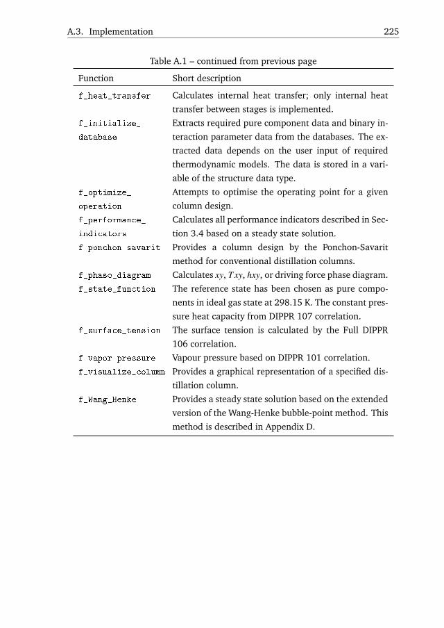
A.3. Implementation 225
Table A.1 – continued from previous page
Function Short description
f_heat_transfer Calculates internal heat transfer; only internal heat
transfer between stages is implemented.
f_initialize_
database
Extracts required pure component data and binary in-
teraction parameter data from the databases. The ex-
tracted data depends on the user input of required
thermodynamic models. The data is stored in a vari-
able of the structure data type.
f_optimize_
operation
Attempts to optimise the operating point for a given
column design.
f_performance_
indicators
Calculates all performance indicators described in Sec-
tion 3.4 based on a steady state solution.
f_ponchon_savarit Provides a column design by the Ponchon-Savarit
method for conventional distillation columns.
f_phase_diagram Calculates xy, T xy, hxy, or driving force phase diagram.
f_state_function The reference state has been chosen as pure compo-
nents in ideal gas state at 298.15 K. The constant pres-
sure heat capacity from DIPPR 107 correlation.
f_surface_tension The surface tension is calculated by the Full DIPPR
106 correlation.
f_vapor_pressure Vapour pressure based on DIPPR 101 correlation.
f_visualize_column Provides a graphical representation of a specified dis-
tillation column.
f_Wang_Henke Provides a steady state solution based on the extended
version of the Wang-Henke bubble-point method. This
method is described in Appendix D.

226 Appendix A. Model Impelementation Documentation
f_activity_coefficient
f_activity_coefficient_UNIFAC
f_activity_coefficient_UNIQUAC
f_activity_coefficient_Wilson
f_check_loading
f_column
f_column_definitions
f_comp2idx
f_density
f_design_column
f_design_internals
f_equilibrium_constant
f_fenske_underwood_gililand
f_fit_binary
f_flash
f_flow
f_fugacity_coefficient
f_fugacity_coefficient_SRK
f_heat_transfer
f_initialize_database
f_optimize_operation
f_ponchon_savarit
f_state_function
f_performance_indicators
f_phase_diagram
f_surface_tension
f_vapor_pressure
f_Wang_Henkef_visualize_column
f_visualize_designUSER
DATABASEPure component parameters
D_PureComponentDatabase.xlsx
DATABASEBinary interaction parameters
d_UNIFAC1p.xlsxd_UNIQUAC.xlsx
d_Wilson.xlsx
Figure A.1. Model implementation hierarchy illustrating the links between theMatlab functions listed in Table A.1.

AppendixB
Mathematical Derivations
The mathematical derivations applied throughout the thesis are collected in this
appendix.
B.1 State Functions
The ideal vapour enthalpy of a pure component at temperature T is obtained by
mathematical integration of the constant pressure heat capacity (cVP,i, j):
hVi, j =
∫ Ti
T=Tre f
cVP,i, jdT
=
[A jT +
B jC j cosh(C j/T )sinh(C j/T )
− D jE j sinh(E j/T )cosh(E j/T )
]Ti
T=Tre f
Similarly, the vapour entropy of a pure component at temperature T is obtained by
mathematical integration:
sVi, j =
∫ Ti
T=Tre f
cVP,i, j
TdT
=[A lnT +D j ln
(e2E j/T +1
)−B j ln
(e2C j/T −1
)+
2C jB j
T
(1
e2C j/T −1+1)
+2E jD j
T
(1
e2E j/T +1−1)]Ti
T=Tre f

228 Appendix B. Mathematical Derivations
The ideal liquid constant pressure heat capacity can be obtained through differen-
tiation:
cLP,i, j =
∂
∂T∆vaphi, j
=−2B jC2
j
T 3i sinh(C j/Ti)
2 +2B jC3
j cosh(C j/Ti)
T 4i sinh(C j/Ti)
3
−2D jE2
j
T 3i cosh(E j/Ti)
2 +2D jE3
j sinh(E j/Ti)
T 4i cosh(E j/Ti)
3
B.2 Derivatives Chain Rule Algebra
Following approach is employed for converting liquid energy holdup derivatives
into temperature derivatives. The liquid is assumed to be incompressible, which
implies uLj = hL
j . Hence:
ddt(uLML
T ) =ddt(hLML
T )
=MLT
dhL
dt+hL dML
Tdt
The time derivative of the enthalpy is:
dhL
dt=
ddt
NC
∑j=1
x jhLj
=NC
∑j=1
(hL
jdx j
dt+ x j
dhLj
dt
)
=NC
∑j=1
(hL
jdx j
dt+ x jcL
P, jdTdt
)Here the chain rule was used:
dhLj
dt=
∂hLj
∂TdTdt
= cLP, j
dTdt
(B.1)
was substituted. The energy holdup derivatives can thus be expressed in tempera-
ture derivatives:
dTdt
=1
CLP
(ddt(hLML
T )−MLT
NC
∑j=1
hLjdx j
dt+hL d
dTML
T
)(B.2)
When the vapour phase energy holdup derivatives must be expressed in terms
of temperature derivatives, one has to account for the relation between enthalpy
and internal energy u = h−PV . Thus, the internal energy derivative of a vapour
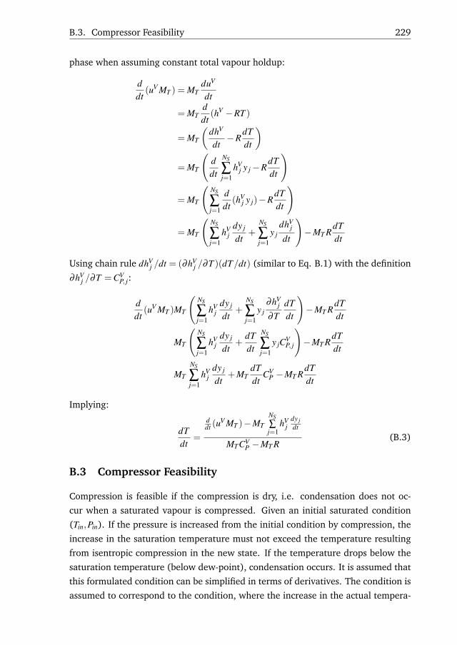
B.3. Compressor Feasibility 229
phase when assuming constant total vapour holdup:
ddt(uV MT ) = MT
duV
dt
= MTddt(hV −RT )
= MT
(dhV
dt−R
dTdt
)= MT
(ddt
NS
∑j=1
hVj y j−R
dTdt
)
= MT
(NS
∑j=1
ddt(hV
j y j)−RdTdt
)
= MT
(NS
∑j=1
hVj
dy j
dt+
NS
∑j=1
y jdhV
j
dt
)−MT R
dTdt
Using chain rule dhVj /dt = (∂hV
j /∂T )(dT/dt) (similar to Eq. B.1) with the definition
∂hVj /∂T =CV
P, j:
ddt(uV MT )MT
(NS
∑j=1
hVj
dy j
dt+
NS
∑j=1
y j∂hV
j
∂TdTdt
)−MT R
dTdt
MT
(NS
∑j=1
hVj
dy j
dt+
dTdt
NS
∑j=1
y jCVP, j
)−MT R
dTdt
MT
NS
∑j=1
hVj
dy j
dt+MT
dTdt
CVP −MT R
dTdt
Implying:
dTdt
=
ddt (u
V MT )−MTNS∑j=1
hVj
dy jdt
MTCVP −MT R
(B.3)
B.3 Compressor Feasibility
Compression is feasible if the compression is dry, i.e. condensation does not oc-
cur when a saturated vapour is compressed. Given an initial saturated condition
(Tin,Pin). If the pressure is increased from the initial condition by compression, the
increase in the saturation temperature must not exceed the temperature resulting
from isentropic compression in the new state. If the temperature drops below the
saturation temperature (below dew-point), condensation occurs. It is assumed that
this formulated condition can be simplified in terms of derivatives. The condition is
assumed to correspond to the condition, where the increase in the actual tempera-
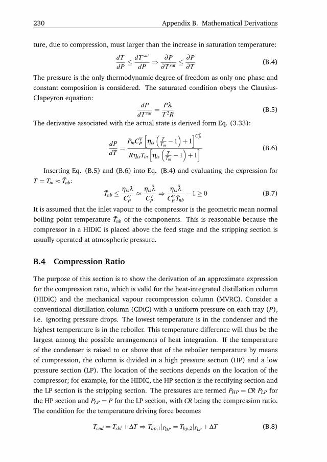
230 Appendix B. Mathematical Derivations
ture, due to compression, must larger than the increase in saturation temperature:
dTdP≤ dT sat
dP⇒ ∂P
∂T sat ≤∂P∂T
(B.4)
The pressure is the only thermodynamic degree of freedom as only one phase and
constant composition is considered. The saturated condition obeys the Clausius-
Clapeyron equation:dP
dT sat =Pλ
T 2R(B.5)
The derivative associated with the actual state is derived form Eq. (3.33):
dPdT
=PinCV
P
[ηis
(TTin−1)+1]CV
P
RηisTin
[ηis
(TTin−1)+1] (B.6)
Inserting Eq. (B.5) and (B.6) into Eq. (B.4) and evaluating the expression for
T = Tin ≈ Tnb:
Tnb ≤ηisλ
CVP≈ ηisλ
CVP⇒ ηisλ
CVP Tnb
−1≥ 0 (B.7)
It is assumed that the inlet vapour to the compressor is the geometric mean normal
boiling point temperature Tnb of the components. This is reasonable because the
compressor in a HIDiC is placed above the feed stage and the stripping section is
usually operated at atmospheric pressure.
B.4 Compression Ratio
The purpose of this section is to show the derivation of an approximate expression
for the compression ratio, which is valid for the heat-integrated distillation column
(HIDiC) and the mechanical vapour recompression column (MVRC). Consider a
conventional distillation column (CDiC) with a uniform pressure on each tray (P),
i.e. ignoring pressure drops. The lowest temperature is in the condenser and the
highest temperature is in the reboiler. This temperature difference will thus be the
largest among the possible arrangements of heat integration. If the temperature
of the condenser is raised to or above that of the reboiler temperature by means
of compression, the column is divided in a high pressure section (HP) and a low
pressure section (LP). The location of the sections depends on the location of the
compressor; for example, for the HIDIC, the HP section is the rectifying section and
the LP section is the stripping section. The pressures are termed PHP = CR PLP for
the HP section and PLP = P for the LP section, with CR being the compression ratio.
The condition for the temperature driving force becomes
Tcnd = Trbl +∆T ⇒ Tbp,1|PHP = Tbp,2|PLP +∆T (B.8)
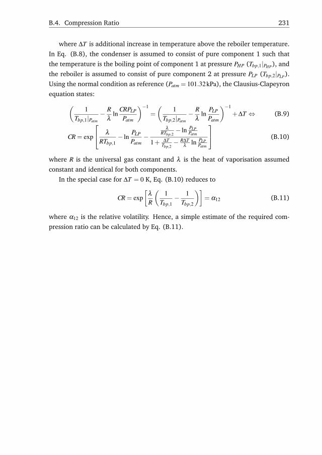
B.4. Compression Ratio 231
where ∆T is additional increase in temperature above the reboiler temperature.
In Eq. (B.8), the condenser is assumed to consist of pure component 1 such that
the temperature is the boiling point of component 1 at pressure PHP (Tbp,1|PHP), and
the reboiler is assumed to consist of pure component 2 at pressure PLP (Tbp,2|PLP).
Using the normal condition as reference (Patm = 101.32kPa), the Clausius-Clapeyron
equation states:(1
Tbp,1|Patm
− Rλ
lnCRPLP
Patm
)−1
=
(1
Tbp,2|Patm
− Rλ
lnPLP
Patm
)−1
+∆T ⇔ (B.9)
CR = exp
λ
RTbp,1− ln
PLP
Patm−
λ
RTbp,2− ln PLP
Patm
1+ ∆TTbp,2− R∆T
λln PLP
Patm
(B.10)
where R is the universal gas constant and λ is the heat of vaporisation assumed
constant and identical for both components.
In the special case for ∆T = 0 K, Eq. (B.10) reduces to
CR = exp[
λ
R
(1
Tbp,1− 1
Tbp,2
)]= α12 (B.11)
where α12 is the relative volatility. Hence, a simple estimate of the required com-
pression ratio can be calculated by Eq. (B.11).


AppendixC
Supplementary Material for EconomicModel
The values of the Souder-Brown factor, presented in the book of Biegler et al. [9],
has been read off and implemented as a look-up table in the Matlab implementa-
tion. An illustration generated by the look-up table is shown in Figure C.1.
10−2 10−1 10010−1.5
10−1
10−0.5
LMW L
V MWV
(ρV
ρL
)0.5
Csb=
u( ρ
V
ρL−
ρV
) 0.5 (20 σ
) 0.2
Figure C.1. Souder-Brown factor for column internals [9].


AppendixD
Extended BPMethod
The BP Method [163] provides a readily programmed, rapid solution procedure for
a certain set of input specifications. By using temperatures and vapour flow rates
as tear variables, all mass-energy-sum-enthalpy balances (MESH) can be solved se-
quentially. In particular, the mass balances w.r.t. the liquid mole fractions become
linear and thus a tridiagonal matrix is obtained. This tridiagonal matrix is then
solved by a modified Gaussian-elimination algorithm referred to as the Thomas Al-
gorithm. The BP Method has been extended by including an extra step that handles
internal heat integration. However, as temperatures are tear variables this step
becomes straight forward. The Extended BP Method is illustrated in Figure D.1.
Step 1: Specify degrees of freedom
The specifications are:
• Feed temperature (TF), pressure (PF), composition (zF), and enthalpy (hF)
and stage locations (NF)
• Stage pressures (Pi) for i = 1,2, . . . ,NS. Specifying the stage pressures also
dictates the positions of the comperssor/throttling valves.
• Flow rate of liquid sidestreams (Ui) and vapour sidestreams (Wi) for i =
1,2, . . . ,NS. Note that the distillate flow rate is designed as U1.
• External heat transfer rates (Qi) at all stages but the first (condenser) and the
last (reboiler), i.e. for i = 2,3, . . . ,NS−1
• Total number of stages (NS)
• Reflux ratio (RR = L1/U1)

236 Appendix D. Extended BP Method
Initialize tear variables
Ti(0), Vi(0)
Compute xi,j from Thomas
method
Normalize xi,j
Compute new Ti from
bubble point equation and
yi,j
Compute configuration
specific variables
Compute Vi and Li from
matrix substitution
method
Is the error below
tolerance?
Adjust tear
variables
Ti(k), Vi(k)
Yes
Converged
No
Not
converged
k:=k+1
Next
iteration
Exit
Specify all Fi, zi,j, hF,i, Pi, Ui, Wi, and
configuration specific degrees of freedom
Figure D.1. Extended BP Algorithm.
• Top vapour flow rate (V1)
• The pairing of heat-integrated stages (see Section 3.3.4)

237
Step 2: Initialise tear variables
The tear variables are Vi and Ti for all NS stages. For conventional distillation
columns, it is sufficient to initialise the tear variables using linear interpolation of
top and bottom bubble-point temperatures based on the specified product compo-
sitions, and by assuming constant-molar interstage flows for the vapour flow rates.
In this work, the initialisation is carried out as described below.
A uniform temperature initialisation has been employed based on averaged feed
conditions:
Ti = Tbp|Pi,z, i = 1,2, . . . ,NS (D.1)
where
Tbp = bubble point [K]
Pi = specified stage pressure [kPa]
z = averaged feed composition [-]
Using the temperature initialisation in Eq. (D.1), internal heat integration can be
included in the initialisation of the vapour flow, as a higher temperature is obtained
through the pressure variations. The vapour flow rate profile can thus be initialised
using:
Vi = (U1−L1)+NS
∑k=i
(Fk(1−qk)+
qk
∆hvap,k
), i = 2,3, . . . ,NS (D.2)
where
∆hvap,k = heat of vaporisation at the specified conditions and temperature
from eq. (D.1).
Step 3: Compute x from tridiagonal matrix algorithm
Due to the tridiagonal matrix structure, the mass balances can be solved succes-
sively starting from the top stage (i = 1):
Bi, j =−(Vi+1 + ∑k=1
i(−V1 +Fk−Wk−Uk)+(Vi +Wi)Ki, j (D.3)
Ci, j =Vi+1Ki+1, j (D.4)
Di, j =−Fizi, j (D.5)
pi, j =C j
B j(D.6)
qi, j =D j
B j(D.7)

238 Appendix D. Extended BP Method
From stage i = 2,3, . . . ,NS−1:
Ai =Vi +i−1
∑k=1
(Fk−Wk−Uk) (D.8)
Bi, j =−[
Vi+1 +i
∑k=1
(Fi−Wi−Ui)+Ui +(Vi +Wi)Ki, j
](D.9)
Ci, j =Vi+1Ki+1, j (D.10)
Di, j =−Fizi, j (D.11)
pi, j =Ci, j
Bi, j−Ai pi−1, j(D.12)
qi, j =Di, j−Aiqi−1, j
Bi, j−Ai pi−1, j(D.13)
And the last stage i = NS:
Ai ==Vi +i−1
∑k=1
(Fk−Wk−Uk) (D.14)
Bi, j =−[
i
∑k=1
(Fk−Wk−Uk)+U(i)+(Vi +Wi)Ki, j
](D.15)
Di, j =−Fi ∗ zi, j (D.16)
qi, j =Di, j−Aiqi−1, j
Bi, j−Ai pi−1, j(D.17)
The liquid mole fraction can be obtained successively starting running in reverse
order from i = NS,NS−1, . . . ,1:
xNS, j = qNS, j (D.18)
xi, j = qi, j− pi, jxi+1, j, i = NS−1,NS−2, . . . ,1 (D.19)
Note that the equilibrium factors of each component at stage i is obtained using the
state of the previous iteration K(k) = f (T (k−1),P(k−1),x(k−1),y(k−1)).
Step 4: Normalise x
The liquid mole fractions are normalised according to the formula:
xi, j :=xi, j
NC∑
k=1xi,k
(D.20)
The normalisation requires the mole fractions to be updated, and therefore the
operator ":=" meaning "replaced by".
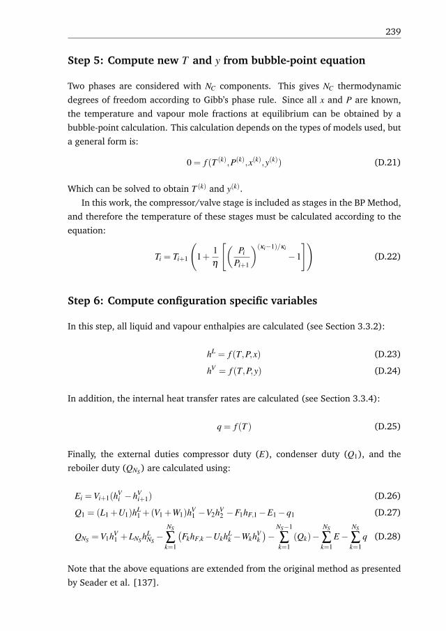
239
Step 5: Compute new T and y from bubble-point equation
Two phases are considered with NC components. This gives NC thermodynamic
degrees of freedom according to Gibb’s phase rule. Since all x and P are known,
the temperature and vapour mole fractions at equilibrium can be obtained by a
bubble-point calculation. This calculation depends on the types of models used, but
a general form is:
0 = f (T (k),P(k),x(k),y(k)) (D.21)
Which can be solved to obtain T (k) and y(k).
In this work, the compressor/valve stage is included as stages in the BP Method,
and therefore the temperature of these stages must be calculated according to the
equation:
Ti = Ti+1
(1+
1η
[(Pi
Pi+1
)(κi−1)/κi
−1
])(D.22)
Step 6: Compute configuration specific variables
In this step, all liquid and vapour enthalpies are calculated (see Section 3.3.2):
hL = f (T,P,x) (D.23)
hV = f (T,P,y) (D.24)
In addition, the internal heat transfer rates are calculated (see Section 3.3.4):
q = f (T ) (D.25)
Finally, the external duties compressor duty (E), condenser duty (Q1), and the
reboiler duty (QNS) are calculated using:
Ei =Vi+1(hVi −hV
i+1) (D.26)
Q1 = (L1 +U1)hL1 +(V1 +W1)hV
1 −V2hV2 −F1hF,1−E1−q1 (D.27)
QNS =V1hV1 +LNS hL
NS−
NS
∑k=1
(FkhF,k−UkhL
k −WkhVk)−
NS−1
∑k=1
(Qk)−NS
∑k=1
E−NS
∑k=1
q (D.28)
Note that the above equations are extended from the original method as presented
by Seader et al. [137].

240 Appendix D. Extended BP Method
Step 7: Compute V and L from matrix substitution method
The liquid and vapour flow rates are updated using energy balances:
αi = hLi−1−hV
i (D.29)
βi = hVi+1−hL
i (D.30)
γi =i−1
∑k=1
(−V1 +Fk−Wk−Uk)(hL
i −hLi−1)+Fi(hL
i −hF,i)+Wi(hVi −hL
i )−Qi−qi−Ei−UihLi
(D.31)
Vi+1 =γi−αi ∗Vi
βi(D.32)
Li =Vi+1 +i
∑k=1
(−V1 +Fk−Wk−Uk) (D.33)
Step 8: Evaluate tolerance
The iteration stop criterion:
1NS
(NS
∑i=1
[T (k)
i −T (k−1)i
T (k)i
]+
NS
∑i=1
[V (k)
i −V (k−1)i
V (k)i
])≤ ε (D.34)
In this work, the tolerance ε = 10−8. If the criteria in Eq. (D.34) is not satisfied, the
iteration number (k) is increased by one and the algorithm is repeated from Step
2.

AppendixE
Design Method Comparison
This appendix serves as a comparison of the presented design method in Chapter
4 to existing design methods. The employed existing methods are the Ponchon-
Savarit method [56] and the Extended Ponchon-Savarit method [159].
Detailed descriptions of the individual, reviewed design methods are not pro-
vided in this section, but their steps are systematically described in relation to the
considered separation. For derivation and further information on the design meth-
ods see the provided references along with the reviews. For a basis of comparison,
the separation of methanol/water with the specifications listed in Table E.1. This
binary mixture has a non-ideal behaviour as a result of hydrophilic interactions,
which is expected to result in column design with column sections of different sizes.
As the heat-integrated pairs of the column stages is an essential element in a design
method of a HIDiC, the design outcomes from the two considered methods should
be compared. In addition, the separation is sufficiently easy such that it can be
carried out in a reasonably low amount of stages. Therefore graphical methods can
be easily represented with sufficient readability.
Table E.1. Separation for testing the design methods.
Variable Unit ValueComponents - Methanol/waterVLE Model - UNIFAC 1p VLEFeed flow rate mols−1 69.4Composition - 0.58Feed pressure kPa 101.3Feed temperature K 344.85Distillate composition - 0.9Bottoms composition - 0.1
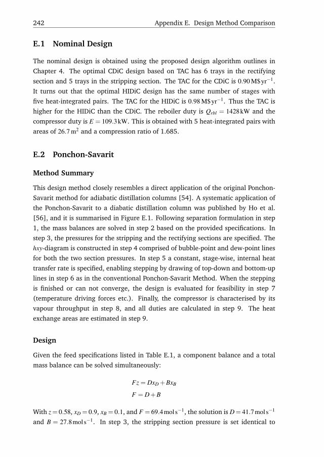
242 Appendix E. Design Method Comparison
E.1 Nominal Design
The nominal design is obtained using the proposed design algorithm outlines in
Chapter 4. The optimal CDiC design based on TAC has 6 trays in the rectifying
section and 5 trays in the stripping section. The TAC for the CDiC is 0.90 M$yr−1.
It turns out that the optimal HIDiC design has the same number of stages with
five heat-integrated pairs. The TAC for the HIDiC is 0.98 M$yr−1. Thus the TAC is
higher for the HIDiC than the CDiC. The reboiler duty is Qrbl = 1428kW and the
compressor duty is E = 109.3kW. This is obtained with 5 heat-integrated pairs with
areas of 26.7 m2 and a compression ratio of 1.685.
E.2 Ponchon-Savarit
Method Summary
This design method closely resembles a direct application of the original Ponchon-
Savarit method for adiabatic distillation columns [54]. A systematic application of
the Ponchon-Savarit to a diabatic distillation column was published by Ho et al.
[56], and it is summarised in Figure E.1. Following separation formulation in step
1, the mass balances are solved in step 2 based on the provided specifications. In
step 3, the pressures for the stripping and the rectifying sections are specified. The
hxy-diagram is constructed in step 4 comprised of bubble-point and dew-point lines
for both the two section pressures. In step 5 a constant, stage-wise, internal heat
transfer rate is specified, enabling stepping by drawing of top-down and bottom-up
lines in step 6 as in the conventional Ponchon-Savarit Method. When the stepping
is finished or can not converge, the design is evaluated for feasibility in step 7
(temperature driving forces etc.). Finally, the compressor is characterised by its
vapour throughput in step 8, and all duties are calculated in step 9. The heat
exchange areas are estimated in step 9.
Design
Given the feed specifications listed in Table E.1, a component balance and a total
mass balance can be solved simultaneously:
Fz = DxD +BxB
F = D+B
With z= 0.58, xD = 0.9, xB = 0.1, and F = 69.4mols−1, the solution is D= 41.7mols−1
and B = 27.8mols−1. In step 3, the stripping section pressure is set identical to
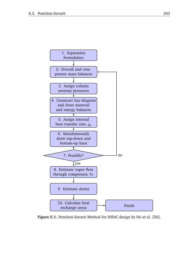
E.2. Ponchon-Savarit 243
1. Separationformulation
2. Overall and com-ponent mass balances
3. Assign columnsections pressures
4. Construct hxy-diagramand draw material
and energy balances
5. Assign internalheat transfer rate, qn
6. Simultaneouslydraw top-down and
bottom-up lines
7. Feasible?
8. Estimate vapor flowthrough compressor, VF
9. Estimate duties
10. Calculate heatexchange areas Finish
yes
no
Figure E.1. Ponchon-Savarit Method for HIDiC design by Ho et al. [56].

244 Appendix E. Design Method Comparison
the feed pressure Pstr = 101.3kPa. It is recommended that the rectifying section
pressure is selected such that the temperature difference between the dew point
temperature of the top product and the bubble-point temperature of the bottoms
product should be significant. A minimum temperature difference of 10 K is sug-
gested by the authors. The bubble-point temperature of the bottoms product is
360.8 K. For the same separation, Ho et al. [56] propose a rectifying section pres-
sure of 202.6 kPa. However, at this pressure the dew-point temperature of the top
product is only 360.1 K and does not fulfil the suggested minimum temperature dif-
ference. By manual iterations, a rectifying section pressure of 350 kPa was found to
be satisfactory giving a minimum temperature difference of 15.6 K. The equilibrium
data are represented in an hxy-diagram in step 4 along with lines representing the
overall mass and energy balances. Using this line, the sum of the compressor and
the reboiler duties divided by the bottoms flow rate can be estimated, obtaining
(E +Qrbl)/B = 56.8kJmol−1. As a result E +Qrbl = 1578kW. The minimum overall
heat transfer rate (qminHT = 504.3kW) is estimated graphically in order to provide in-
sights in selecting the internal heat transfer rate later in the following step. Based on
the minimum overall heat transfer rate, a value of internal heat transfer qn = 150kWis chosen. No direct guidelines for selecting qn is provided and iterations of this vari-
able might be necessary for obtaining a feasible design. A design pinch is reached
if work and equilibrium lines become parallel, which leads to an infeasible design
and adjustments in design are required. In step 6, the simultaneously top-down
and bottom up lines drawing is performed. The construction of the lines is carried
out by alternating between equilibrium and work lines, which are straight lines.
The work lines are shifted by a vertical distance proportional to the internal heat
transfer q/B = 5.4kJmol−1. The resulting design has four heat-integrated pairs with
five trays in the rectifying section and four trays in the stripping section. The tem-
perature driving forces of the four pairs are estimated as 13.8 K, 23.2 K, 27.8 K,
and 30.0 K from top to bottom, leading to heat exchange areas of 18.2 m2, 10.8 m2,
9.0 m2, and 8.4 m2 using U = 0.60kWm−2 K−1. The vapour flow through the com-
pressor is estimated in step 8 using the component and overall mass balances of the
rectifying section:
0 =VF −LR1−D
0 =VF yF −LR1xR1−DyT
Using D= 41.7mols−1, yT = 0.9 and by reading xR = 0.64 and yF = 0.81 from the hxy-
diagram, LR1 = 23.6mols−1 and VF = 65.3mols−1 result. The latter, VF = 65.3mols−1,
is the vapour flow through the compressor.
The compressor duty (E) is calculated using eq. (2.2). Inserting the values

E.2. Ponchon-Savarit 245
−0.1 0 0.1 0.2 0.3 0.4 0.5 0.6 0.7 0.8 0.9 1 1.1
−350
−300
−250
−200
−150
x,y
hL,h
V
Figure E.2. HIDiC design obtained by the Ponchon-Svararit method.
κ = 1.23, R = 0.008314kJmol−1 K−1, Pout = 350.0kPa, Pin = 101.3kPa, TNF = 345K,
and the vapour flow through the compressor from step 8, a duty of E = 261.2kW is
obtained. The reboiler duty is hence obtained by subtracting compressor duty from
the overall heat duty obtained in step 4, giving Qrbl = 1317kW.
Results and Discussion
With the hxy-diagram and the corresponding final column design in Figure E.2,
the Ponchon-Savarit Method has provided a feasible HIDiC design. The Ponchon-
Savarit method provides a relatively simple, graphical approach for HIDiC design.
However, the method only serves as a means to give a rapid feasible solution (esti-
mating duties) and is therefore not suited for fine-tuning the design as the stepping
in the hxy-diagram is time consuming. This is also a impractical if iterations are
required. The major limitations of the design method is that it does not supply any
generic guidelines for selecting the compression ratio, the pairing of the stages, and
at which stages internal heat integration should take place.

246 Appendix E. Design Method Comparison
E.3 Extended Ponchon-Savarit
Method Summary
Wakabayashi and Hasebe [159] claimed to address the weaknesses of the method
by Ho et al. [56] in a method referred to as the Extended Ponchon-Savarit Method.
The method starts with separation formulation in step 1 and the full procedure is
summarised in Figure E.3. The HIDiC design takes its starting point (step 2) in a
conventional distillation column design. In step 3, the number of stages in the two
column sections will provide insights for specifying bounds of these values, whereas
the reboiler duty of the conventional distillation provides a reasonable estimate of
the required hot utilities. For example a specification of a HIDiC reboiler duty could
be half that of a CDiC. The specification of the compressor duty depends on expe-
rience. In addition, the number of pairings must be specified. The ideal conditions
for heat exchange in the stripping section (reversible distillation curves, RDC) are
calculated in step 4, followed by a specification of internal heat integration duties
and drawing of bottom-up lines in step 5. Step 6 ensures that the stripping section
design is in accordance to the desired design as specified in step 3. The rectifying
section is designed using top-down lines in steps 7-9 as in steps 4-6 resulting in de-
sign of the rectifying section. Finally, in step 10, the required heat exchange areas
are calculated.
Design
A column pressure of 101.3 kPa is selected based on the feed pressure. Ponchon-
Savarit stepping for a CDiC is carried out using a reflux ratio to minimum reflux
ratio of 1.2 resulting in 4 stages in both column sections and a reboiler duty of
QCDiCrbl = 2054kW. In step 3, based on the CDiC design, the range of number of
stages in the stripping and rectifying sections are specified as 2 ≤ Nstr ≤ 6 and
2 ≤ Nrct ≤ 6. In addition, a compressor duty of E = 250kW and an energy saving
of 40% corresponding to 822 kW is assumed. Hence, the reboiler duty of the HIDiC
is Qrbl = 1232kW. These numbers are in the same order of the obtained design us-
ing the Ponchon-Savarit Method as described previously. The ideal ideal conditions
for heat exchange in the stripping section are calculated in step 4. The reversible
distillation curves (RDC) are plotted along with the hxy data and are used as a tool
for selecting the ideal heat-integrated stages in both sections. Since a distillation
column has a finite number of stages, the RDC is approximated by the "operating
locus". The drawing of the operating locus is a part of the HIDiC design proce-
dure, and it is drawn such that the vertical distance between itself and the RDC

E.3. Extended Ponchon-Savarit 247
1. Separationformulation
2. Design andsimulate CDiC
3. Specify designtargets (Nrct and Nstrranges, Nihx, Qrbl , E)
4. Calculate idealconditions for heatexchange in strip-
ping section (RDC)
5. Decision of pairedstages in strippingsection and drawbottom-up lines
6. Nstr within bounds?
7. Calculate idealconditions for heatexchange in rectify-ing section (RDC)
8. Decision of pairedstages in rectify-ing section and
draw top-down lines
9. NT within bounds?
10. Calculate heatexchange areas Finish
yes
no
yes
no
Figure E.3. Extended Ponchon-Savarit Method for HIDiC design by Wakabayashiand Hasebe [159].

248 Appendix E. Design Method Comparison
must be approximately the same at any composition. The rectifying section RDC is
shifted by an additional heat input to the stripping section, ∆h = 20kJmol−1 to ob-
tain a shifted RDC (S-RDC). In the composition ranges where the operating locus is
horizontal, the corresponding stages are adiabatic, whereas a vertical displacement
corresponds to a diabatic stages. The operating locus for the stripping section is
obtained by following the rules provided, which results in 3 heat-integrated stages
in the stripping section. The resulting duties are q3 = 222kW, q2 = 333kW, and
q3 = 333kW. The construction of the bottom-up lines are carried out by letting
the operating locus determine the position of the heat-integrated stages. A total
of 6 stages in the stripping section are resulted with the 3 stages below the feed
stage being heat-integrated. The obtained Nstr = 6 is within the bounds specified
in step 3. Based on the defined compressor duty, the rectifying section pressure
must be established for step 7. The vapour flow through the compressor consists
of several contributions [159]: The top vapour leaving the stripping section, the
vapour fraction caused by flashing the feed at the stripping section pressure, and
the vapour fraction cased by flashing the bottoms liquid from the rectifying section
at the stripping section pressure. The following balances are solved for the stripping
section:
0 = Lstr,in−Vstr,out −B
0 = Lstr,inxstr,in−Vstr,outystr,out −BxB
0 = Lstr,inhLstr,in−Vstr,outhV
str,out −BhLB +
Nihx
∑i=1
qi +Qrbl
By using xstr,in = 0.58 and hLstr,in = −254kJmol−1 assumed from feed, with hL
B =
−276kJmol−1, hVstr,out =−207kJmol−1, and ∑Nihx
i=1 qi = 888kW, one obtain L= 85.2mols−1,
V = 57.4mols−1, and y = 0.81. hVstr,out is the vapour enthalpy at the same condition
of the liquid stream entering the stripping section (xstr,in, hLstr,in). Assuming a recti-
fying section pressure of Prct = 350.0kPa, the distribution of the two phases of the
throttled liquid is estimated, as the enthalpy is the intersection of the feed equilib-
rium line and the bubble-point line at 350.0 kPa. The overall composition is 0.616
with the enthalpy of −248.4 kJmol−1. Carrying out a flash calculation a vapour
fraction of 0.108 is obtained and thus the vapour contribution from the throttled
liquid is 0.108/(1− 0.108) · 85.2mols−1 = 10.3mols−1. The contribution from flash-
ing the feed stream is zero since it is a saturated liquid. The vapour flow through
the compressor is thus VS1 = 67.7mols−1. Using equation (2.2) with the estimated
compressor throughput and the values from step 8-9 in the Ponchon-Savarit method
by Ho et al. [56], a pressure, Pout = 320.2kPa is obtained. In step 7, The RDC of the
rectifying section is constructed. The S-RDC for the rectifying section is uniquely

E.3. Extended Ponchon-Savarit 249
determined by passing through the point, obtained by extrapolating the total mass
balance to the distillate composition. The operating locus for the rectifying section
is also constructed based on provided guidelines. The top-down lines are drawn
and 3 stages are resulted excluding the condenser. It is found that the condenser
must be paired with two stages in the rectifying section whereas the 2nd stage must
also be heat-integrated. The obtained Nrct = 3 is within the bounds specified in step
3. In step 10, the heat exchange areas are calculated resulting in 18.3 m2, 19.5 m2,
and 14.4 m2.
Results and Discussion
The graphical solution is presented in figure E.4. The resulting design is more com-
plicated in the sense that heat integration does not take place in the same vertical
height. In fact, the user must specify how many heat-integrated pairs the solution
must contain. This can be both a strength and a weakness. This is because novel
configurations can be obtained, but the arrangement of the heat integration is re-
stricted to stabbed-in type heat exchangers. This has proven useful in an industrial
set-up [161]. A useful aspect of the method is that the impact of different design de-
cisions can be investigated, while maintaining the energy savings constant as these
are specified in Step 3. However, when specifying the energy savings, feasibility can
not always be ensured.

250 Appendix E. Design Method Comparison
−0.1 0 0.1 0.2 0.3 0.4 0.5 0.6 0.7 0.8 0.9 1 1.1
−350
−300
−250
−200
−150
x,y
hL,h
V
Figure E.4. HIDiC design obtained by the extended Ponchon-Svararit method.

AppendixF
Notation
Symbol Definition Unit
Roman symbolsAihx Internal heat exchange area m2
Aa Active tray area m2
ACT Concentric total cross sectional area m2
Ad Downcomer area m2
Ap Perforations area m2
At Tray area m2
AT Total cross sectional area m2
b Availability function kJmol−1
cLP Constant pressure heat capacity of liquid kJmol−1 K−1
cVP Constant pressure heat capacity of vapour kJmol−1 K−1
CR Compression ratio -
d Column diameter me Controller error Varies
E Electrical energy flow rate kWf Mass flow rate kgs−1
fF Feed thermal condition -
F Feed flow rate mols−1
FF Flooding factor -
g Gravitation constant ms−2
hL Enthalpy of liquid kJmol−1
hV Enthalpy of vapour kJmol−1
Continued on next page

252 Appendix F. Notation
Continued from previous page
Symbol Definition Unit
Hcl Clear liquid height mHoW Liquid height over weir mHS Tray spacing mHt Tray thickness mHW Weir height mKc Controller gain Varies
l Column length m
L Liquid flow rate mols−1
M Molar holdup moleMT Total molar holdup moleMW Molecular weight kgmol−1
Ncnd Number of condensers (0 or 1) -
Ncpr Number of compressors -
Nihx Number of heat-integrated stages -
Nrbl Number of reboilers (0 or 1) -
Nrct Number of trays in rectifying section -
NS Number of stages -
Nstr Number of trays in the stripping section
NT Number of trays -
NF Feed stage -
P Pressure kPaPsat Saturated pressure kPaQ External heat transfer rate kWq Internal heat transfer rate kWR Universal gas constant kJmol−1 K−1
RR Reflux ratio -
s Laplace domain independent variable
sL Entropy of liquid kJmol−1 K−1
sV Entropy of vapour kJmol−1 K−1
S Price $kg−1
t Time s
T Temperature KTs Temperature of sink/source KTσ Temperature of surroundings Ku Internal energy kJmol−1
Continued on next page

253
Continued from previous page
Symbol Definition Unit
U Liquid side stream flow rate mols−1
Uhex Overall heat transfer coefficient of a conventional
heat exchanger
Uihx Overall heat transfer coefficient for heat integra-
tion
kgm−2 K−1
v Molar volume m3 mol−1
V Vapour flow rate mols−1
Vrbl Reboiler vapour flow rate mols−1
W Vapour side stream flow rate mols−1
Wlost Lost work kWWmin Minimum work kWx Liquid mole fraction -
y Vapour mole fraction -
ym Measured variable Varies
yset Setpoint Varies
z Feed mole fraction -
Boldface symbolsCV1 Primary controlled variables -
CV2 Secondary controlled variables -
uD Actuators -
x State variables -
y Output vector -
βββ Standard regression coefficient vector -
θθθ Parameter vector -
θθθ∗ Certain parameters -
θθθ ∗ Uncertain parameters -
Greek symbols∆hvap Heat of vaporisation kJmol−1
∆P Pressure drop kPaγ Activity coefficient -
η Efficiency -
θdT Downcomer area per total cross sectional area -
θpa Area of perforations per active tray area -
κ Isentropic expansion factor -
Continued on next page

254 Appendix F. Notation
Continued from previous page
Symbol Definition Unit
λ Constant heat of vaporisation kJmol−1
λ Geometric mean constant heat of vaporisation kJmol−1
ρ Density kgm−3
τc Desired closed-loop time constant sτI Controller integral time sΦ Specific heat transfer area m2 m−3
AbbreviationsBC Bare module cost
CAPEX Capital expenditures
CDiC Conventional distillation column
CE PCI Chemical Engineering Plant Cost Index
cnd Condenser
cpr Compressor
CV Controlled variable
DTI Differential temperature indicator
FOC Feasibility of compression
HIDiC Heat-integrated distillation column
HFI Hydraulic feasibility indicator
ihx Internal heat exchange
LI Level indicator
MF Module factor
MPF Material and pressure correction factor
MV Manipulated variable
MVRC Mechanical vapour recompression column
OC Operating cost
OPEX Operating expenditures
PI Pressure indicator
PID
control
Proportional-integral-derivative control
rbl Reboiler
rct Rectifying section
RTO Real-time optimisation
SRC Standardised regression coefficients
SRVC Secondary reflux and vaporisation column
Continued on next page

255
Continued from previous page
Symbol Definition Unit
TAC Total annualised cost
TPM Throughput manipulator
UBMC Updated bare module cost
VLE Vapour-liquid equilibrium
vlv Throttling valve