operation and monitoring of parabolic trough concentrated

University of South FloridaScholar Commons

Graduate Theses and Dissertations Graduate School

11-4-2015

Operation and Monitoring of Parabolic TroughConcentrated Solar Power PlantHarsha Vardhan AmbaUniversity of South Florida, [email protected]

Follow this and additional works at: http://scholarcommons.usf.edu/etd

Part of the Electrical and Computer Engineering Commons, and the Oil, Gas, and EnergyCommons

This Thesis is brought to you for free and open access by the Graduate School at Scholar Commons. It has been accepted for inclusion in GraduateTheses and Dissertations by an authorized administrator of Scholar Commons. For more information, please contact [email protected].

Scholar Commons CitationAmba, Harsha Vardhan, "Operation and Monitoring of Parabolic Trough Concentrated Solar Power Plant" (2015). Graduate Thesesand Dissertations.http://scholarcommons.usf.edu/etd/5891

http://scholarcommons.usf.edu/?utm_source=scholarcommons.usf.edu%2Fetd%2F5891&utm_medium=PDF&utm_campaign=PDFCoverPages

http://scholarcommons.usf.edu/?utm_source=scholarcommons.usf.edu%2Fetd%2F5891&utm_medium=PDF&utm_campaign=PDFCoverPages

http://scholarcommons.usf.edu?utm_source=scholarcommons.usf.edu%2Fetd%2F5891&utm_medium=PDF&utm_campaign=PDFCoverPages

http://scholarcommons.usf.edu/etd?utm_source=scholarcommons.usf.edu%2Fetd%2F5891&utm_medium=PDF&utm_campaign=PDFCoverPages

http://scholarcommons.usf.edu/grad?utm_source=scholarcommons.usf.edu%2Fetd%2F5891&utm_medium=PDF&utm_campaign=PDFCoverPages

http://scholarcommons.usf.edu/etd?utm_source=scholarcommons.usf.edu%2Fetd%2F5891&utm_medium=PDF&utm_campaign=PDFCoverPages

http://network.bepress.com/hgg/discipline/266?utm_source=scholarcommons.usf.edu%2Fetd%2F5891&utm_medium=PDF&utm_campaign=PDFCoverPages



mailto:[email protected]

Operation and Monitoring of Parabolic Trough Concentrated Solar Power Plant

by

Harsha Vardhan Amba

A thesis submitted in partial fulfillmentof the requirements for the degree of

Master of Science in Electrical EngineeringDepartment of Electrical Engineering

College of EngineeringUniversity of South Florida

Co-Major Professor: E. K. Stefanakos, Ph.D.Co-Major Professor: Wilfrido Moreno, Ph.D.

Yogi Goswami, Ph.D.

Date of Approval:October 22, 2015

Keywords: Sun Tracking, Programmable Logic Controller (PLC), Temperature sensors,Inclinometer, Solar radiation

Copyright © 2015, Harsha Vardhan Amba

DEDICATION

To my loving family and friends for their patience and support.

ACKNOWLEDGMENTS

This work has been supported and funded by the Clean Energy Research Center (CERC) at USF.

I express my most sincere gratitude to my advisors Dr. Lee Stefanakos and Dr. Wilfrido Moreno

for their advice, guidance, and encouragement throughout this work. I am very thankful to Dr.

Yogi Goswami for his tremendous help and serving on my thesis committee. Special thanks to Ms.

Barbara Graham, Dr. Chand Jotshi, and Mr. Charles Garretson who were of great help during my

stay in the Clean Energy Research Center. I would like to thank my friends Sai Bharadwaj and

Janardhan for their help and encouragement throughout this project.

TABLE OF CONTENTS

LIST OF TABLES . . . . . . . . . . . . . . . . . . . . . . . . . . . . . . . . . . . . . . . . . . . . . . . . . . . . . . . . . . . . . . . . . . . . . . . . . . . iii

LIST OF FIGURES . . . . . . . . . . . . . . . . . . . . . . . . . . . . . . . . . . . . . . . . . . . . . . . . . . . . . . . . . . . . . . . . . . . . . . . . . . iv

ABSTRACT . . . . . . . . . . . . . . . . . . . . . . . . . . . . . . . . . . . . . . . . . . . . . . . . . . . . . . . . . . . . . . . . . . . . . . . . . . . . . . . . . vi

CHAPTER 1 : INTRODUCTION . . . . . . . . . . . . . . . . . . . . . . . . . . . . . . . . . . . . . . . . . . . . . . . . . . . . . . . . . . . 11.1 Plant Operation . . . . . . . . . . . . . . . . . . . . . . . . . . . . . . . . . . . . . . . . . . . . . . . . . . . . . . . . . . . . . . . . . 2

CHAPTER 2 : SOLAR RADIATION AND CSP TECHNOLOGIES . . . . . . . . . . . . . . . . . . . . . . . . . 52.1 Introduction . . . . . . . . . . . . . . . . . . . . . . . . . . . . . . . . . . . . . . . . . . . . . . . . . . . . . . . . . . . . . . . . . . . . . 52.2 Solar Radiation . . . . . . . . . . . . . . . . . . . . . . . . . . . . . . . . . . . . . . . . . . . . . . . . . . . . . . . . . . . . . . . . . . 52.3 Current CSP Technologies . . . . . . . . . . . . . . . . . . . . . . . . . . . . . . . . . . . . . . . . . . . . . . . . . . . . . . . 6

2.3.1 Parabolic Trough Systems . . . . . . . . . . . . . . . . . . . . . . . . . . . . . . . . . . . . . . . . . . . . . . 72.3.2 Solar Tower Technology. . . . . . . . . . . . . . . . . . . . . . . . . . . . . . . . . . . . . . . . . . . . . . . . . 92.3.3 Linear Fresnel Collector Systems. . . . . . . . . . . . . . . . . . . . . . . . . . . . . . . . . . . . . . . . 102.3.4 Stirlings Dish Technology . . . . . . . . . . . . . . . . . . . . . . . . . . . . . . . . . . . . . . . . . . . . . . 12

2.4 Conclusion . . . . . . . . . . . . . . . . . . . . . . . . . . . . . . . . . . . . . . . . . . . . . . . . . . . . . . . . . . . . . . . . . . . . . . . 12

CHAPTER 3 : TRACKING SYSTEM DESIGN . . . . . . . . . . . . . . . . . . . . . . . . . . . . . . . . . . . . . . . . . . . . . 153.1 Introduction . . . . . . . . . . . . . . . . . . . . . . . . . . . . . . . . . . . . . . . . . . . . . . . . . . . . . . . . . . . . . . . . . . . . . 15

3.1.1 Module Tracking . . . . . . . . . . . . . . . . . . . . . . . . . . . . . . . . . . . . . . . . . . . . . . . . . . . . . . . 163.2 Tracker Design . . . . . . . . . . . . . . . . . . . . . . . . . . . . . . . . . . . . . . . . . . . . . . . . . . . . . . . . . . . . . . . . . . . 17

3.2.1 Calculating the Sun Path and Angle . . . . . . . . . . . . . . . . . . . . . . . . . . . . . . . . . . . . 173.2.2 Rotating the Collectors to the Sun Angle . . . . . . . . . . . . . . . . . . . . . . . . . . . . . . . 193.2.3 Components Used . . . . . . . . . . . . . . . . . . . . . . . . . . . . . . . . . . . . . . . . . . . . . . . . . . . . . . 193.2.4 Tracker Flowchart . . . . . . . . . . . . . . . . . . . . . . . . . . . . . . . . . . . . . . . . . . . . . . . . . . . . . . 28

CHAPTER 4 : POWER PLANT OPERATION AND MONITORING . . . . . . . . . . . . . . . . . . . . . . . 304.1 Temperature Sensors . . . . . . . . . . . . . . . . . . . . . . . . . . . . . . . . . . . . . . . . . . . . . . . . . . . . . . . . . . . . . 30

4.1.1 Thermocouple . . . . . . . . . . . . . . . . . . . . . . . . . . . . . . . . . . . . . . . . . . . . . . . . . . . . . . . . . . 304.1.2 RTD . . . . . . . . . . . . . . . . . . . . . . . . . . . . . . . . . . . . . . . . . . . . . . . . . . . . . . . . . . . . . . . . . . . 314.1.3 Thermistor . . . . . . . . . . . . . . . . . . . . . . . . . . . . . . . . . . . . . . . . . . . . . . . . . . . . . . . . . . . . . 31

i

4.2 Flow-Loop Hardware . . . . . . . . . . . . . . . . . . . . . . . . . . . . . . . . . . . . . . . . . . . . . . . . . . . . . . . . . . . . . 334.2.1 Flow Meters . . . . . . . . . . . . . . . . . . . . . . . . . . . . . . . . . . . . . . . . . . . . . . . . . . . . . . . . . . . . 334.2.2 Pumps . . . . . . . . . . . . . . . . . . . . . . . . . . . . . . . . . . . . . . . . . . . . . . . . . . . . . . . . . . . . . . . . . 344.2.3 Valves . . . . . . . . . . . . . . . . . . . . . . . . . . . . . . . . . . . . . . . . . . . . . . . . . . . . . . . . . . . . . . . . . . 34

4.3 Operation and Monitoring . . . . . . . . . . . . . . . . . . . . . . . . . . . . . . . . . . . . . . . . . . . . . . . . . . . . . . . 354.3.1 Field Monitoring . . . . . . . . . . . . . . . . . . . . . . . . . . . . . . . . . . . . . . . . . . . . . . . . . . . . . . . 37

CHAPTER 5 : CONCLUSION . . . . . . . . . . . . . . . . . . . . . . . . . . . . . . . . . . . . . . . . . . . . . . . . . . . . . . . . . . . . . . 39

REFERENCES . . . . . . . . . . . . . . . . . . . . . . . . . . . . . . . . . . . . . . . . . . . . . . . . . . . . . . . . . . . . . . . . . . . . . . . . . . . . . . 40

APPENDIXA: PLC PROGRAM . . . . . . . . . . . . . . . . . . . . . . . . . . . . . . . . . . . . . . . . . . . . . . . . . . . . . . . . . . . . 41

ii

LIST OF TABLES

Table 3.1 Input and Outputs Tags for the PLC Program. . . . . . . . . . . . . . . . . . . . . . . . . . . . . . . . . . . . 21

Table 4.1 Temperature Sensors Characteristics . . . . . . . . . . . . . . . . . . . . . . . . . . . . . . . . . . . . . . . . . . . . . 31

iii

LIST OF FIGURES

Figure 1.1 Plant Layout (a) and DNI Data of the Location (b) . . . . . . . . . . . . . . . . . . . . . . . . . . . . . 3

Figure 1.2 USF Powerplant Schematic . . . . . . . . . . . . . . . . . . . . . . . . . . . . . . . . . . . . . . . . . . . . . . . . . . . . . . 3

Figure 2.1 Solar Radiation . . . . . . . . . . . . . . . . . . . . . . . . . . . . . . . . . . . . . . . . . . . . . . . . . . . . . . . . . . . . . . . . . 6

Figure 2.2 Parabolic Trough Technology . . . . . . . . . . . . . . . . . . . . . . . . . . . . . . . . . . . . . . . . . . . . . . . . . . . . 8

Figure 2.3 Solar Tower Technology . . . . . . . . . . . . . . . . . . . . . . . . . . . . . . . . . . . . . . . . . . . . . . . . . . . . . . . . . 10

Figure 2.4 Linear Fresnel Collector Systems . . . . . . . . . . . . . . . . . . . . . . . . . . . . . . . . . . . . . . . . . . . . . . . . 11

Figure 2.5 Stirlings Dish Technology. . . . . . . . . . . . . . . . . . . . . . . . . . . . . . . . . . . . . . . . . . . . . . . . . . . . . . . . 13

Figure 3.1 Functional Block of Solar Position Algorithm . . . . . . . . . . . . . . . . . . . . . . . . . . . . . . . . . . . . 18

Figure 3.2 S7 1200 1214 CPU AC/DC/RLY . . . . . . . . . . . . . . . . . . . . . . . . . . . . . . . . . . . . . . . . . . . . . . . . 20

Figure 3.3 CM 1241 RS 232 Module . . . . . . . . . . . . . . . . . . . . . . . . . . . . . . . . . . . . . . . . . . . . . . . . . . . . . . . . 20

Figure 3.4 SM 1222 RLY Module . . . . . . . . . . . . . . . . . . . . . . . . . . . . . . . . . . . . . . . . . . . . . . . . . . . . . . . . . . . 21

Figure 3.5 T7-1-CAN Inclinometer (Adapted from [1]) . . . . . . . . . . . . . . . . . . . . . . . . . . . . . . . . . . . . . . 22

Figure 3.6 CANA 232 Adapter (Adapted from [2]) . . . . . . . . . . . . . . . . . . . . . . . . . . . . . . . . . . . . . . . . . . 23

Figure 3.7 Single Line Configuration of Inclinometer Network (Adapted from [2]) . . . . . . . . . . . 24

Figure 3.8 Parallel Line Configuration of Inclinometer Network(Adapted from [2]) . . . . . . . . . . 25

Figure 3.9 Speed Controller of Motor . . . . . . . . . . . . . . . . . . . . . . . . . . . . . . . . . . . . . . . . . . . . . . . . . . . . . . . 25

Figure 3.10 Limit Switch . . . . . . . . . . . . . . . . . . . . . . . . . . . . . . . . . . . . . . . . . . . . . . . . . . . . . . . . . . . . . . . . . . . 27

Figure 3.11 DPDT Relay . . . . . . . . . . . . . . . . . . . . . . . . . . . . . . . . . . . . . . . . . . . . . . . . . . . . . . . . . . . . . . . . . . . 27

Figure 3.12 Tracker Block Diagram. . . . . . . . . . . . . . . . . . . . . . . . . . . . . . . . . . . . . . . . . . . . . . . . . . . . . . . . . 28

iv

Figure 4.1 Resistance Temperature Detector Schematic . . . . . . . . . . . . . . . . . . . . . . . . . . . . . . . . . . . . . 32

Figure 4.2 TX92G 4 Temperature Transmitter . . . . . . . . . . . . . . . . . . . . . . . . . . . . . . . . . . . . . . . . . . . . . . 32

Figure 4.3 Flow Meter Schematic . . . . . . . . . . . . . . . . . . . . . . . . . . . . . . . . . . . . . . . . . . . . . . . . . . . . . . . . . . . 33

Figure 4.4 Plant Operation and Maintenance Flowchart . . . . . . . . . . . . . . . . . . . . . . . . . . . . . . . . . . . . 35

Figure 4.5 Power Plant Operation Program. . . . . . . . . . . . . . . . . . . . . . . . . . . . . . . . . . . . . . . . . . . . . . . . . 38

Figure 4.6 SCADA VIEW. . . . . . . . . . . . . . . . . . . . . . . . . . . . . . . . . . . . . . . . . . . . . . . . . . . . . . . . . . . . . . . . . . 38

v

ABSTRACT

The majority of the power generated today is produced using fossil fuels,emitting carbon dioxide and

other pollutants every second. Also, fossil fuels will eventually run out. For the increasing worldwide

energy demand, the use f reliable and environmentally beneficial natural energy sources is one of

the biggest challenges. Alongside wind and water, the solar energy which is clean, CO2-neutral and

limitless, is our most valuable resource.

Concentrated solar power (CSP) is becoming one of the excellent alternative sources for the power

industry. The successful implementation of this technology requires the efficient design of tracking

and operation system of the CSP solar plants. A detailed analysis of components needed for the

design of cost-effective and optimum tracker for CSP solar systems is required for the power plant

modeling, which is the primary subject of this thesis. A comprehensive tracking and operating

system of a parabolic trough solar power plant was developed focusing primarily on obtaining

optimum and cost effective design through the simplified methodology of this work. This new

model was implemented for a 50 kWe parabolic trough solar power plant at University of South

Florida, Tampa.

vi

CHAPTER 1 : INTRODUCTION

The current world energy consumption shows that approximately 80% of the world energy is gener-

ated from fossil fuels, and only 8% is from renewable energies. Total primary energy consumption

grows in Reference case (1980-2040) of the Annual Energy Outlook (AEO)2015 [3] by 8.6 quadrillion

Btu (8.9%), from 97.1 quadrillion Btu in 2013 to 105.7 quadrillion Btu in 2040. Most of the growth

is in consumption of natural gas and renewable energy.[3] Renewable energy sources are very at-

tractive for many reasons such as being environmental friendly, lowering greenhouse gas emissions,

etc. Solar energy is one of the popular forms of renewable energy; there are two ways of generat-

ing energy using sunlight. The most prominent method is using photovoltaic solar cells (PV) that

produce electricity by directly converting photons to electrons using semiconductor materials. By

contrast, Concentrating Solar Power (CSP) reflects sunlight via solar collectors to heat a receiver

to high temperatures. This heat is then transformed first into mechanical energy by turbines or

Stirling engines, and then to electricity.

Photovoltaic cells produce direct current (DC) which must be converted to alternating current using

a grid-tied inverter in existing distribution grids that use AC, This leads to an energy loss of 4 %

to 12 %. Power grids usually prefer CSP over PV’s as most electricity is generated is by the steam

engine that converts heat energy into mechanical energy and then into electrical energy. CSP only

uses the heat engine and does not have the conversion problem, So it can be directly connected to

the grid and equipped with backup power from combustible fuels. CSP has many other advantages

1

over PV such as having higher efficiencies, higher economic return, an inherent thermal storage

capacity that enables power generation, and a better hybrid operation capability. These features

allow CSP to continue to generate power both during cloud cover and at night.

This thesis will focus on the parabolic trough collector CSP system tracking, operation, and mon-

itoring.The work was done for the solar park located on Spectrum Blvd at USF Tampa, which

was built to demonstrate new research in renewable energies, and to help students learn renewable

energy technologies. The electricity generated by this plant is used for USF, and is also fed into the

utilities electricity grid.

The Daily Integration (DI) approach was applied to obtain the average direct normal solar radiation

(DNI) for the location of the solar plant (USF, Tampa, FL). The direct normal solar radiation

obtained for Tampa is shown in Fig. 1., and the average annual DNI for this location is 4.6

kWh/m2-day. These solar radiation values and the solar shading analysis for solar collector rows

were used for the solar field calculation. Fig 1.1 shows the solar field layout of the constructed 50

kWe capacity CSP system.

The Soponova 4.0 collectors from Sopogy Inc parabolic trough collectors were used in the solar field

for generating 430 W/m2 of thermal energy after losses. The solar field was designed to work in

conjunction with a thermal energy storage system that uses phase change materials (PCM) as a

thermal energy storage medium.

1.1 Plant Operation

As shown in the Fig. 1.2 , the circulating cold heat transfer fluid (HTF) passes through the receiver

tube and is heated by the radiant energy absorber, and exits at high temperature. This HTF is

2

Figure 1.1: Plant Layout (a) and DNI Data of the Location (b).

Figure 1.2: USF Powerplant Schematic.

3

passed through preheater, followed by an evaporator, where its heat energy is used to vaporize

working fluid (WF).AS the working fluid expands, it drives a proprietary twin screw expander. The

main rotor of the expander is belt-coupled to an induction generator that produces electricity. After

expansion, the working fluid vapor enters a condenser where it is air cooled and condensed to liquid.

This condensed liquid is passed through a feed pump that raises the pressure of the condensed liquid

and then returns it to the evaporator to repeat the cycle.

4

CHAPTER 2 : SOLAR RADIATION AND CSP TECHNOLOGIES

2.1 Introduction

Due to the increasing worldwide energy demand, finding reliable and environmentally beneficial

uses of natural energy resources is the biggest challenge of this generation. A majority the power

being today is produced by fossil fuels, which emit carbon dioxide and other pollutants into the

environment. Also these fossil fuels run out eventually. For the increasing demands in clean energy,

solar energy is one of the fastest growing resources of future energy requirement. There are different

types of solar technologies available in the market. For example, photovoltaic systems (PV) converts

the sun heat energy directly into electrical energy while concentrated solar power (CSP) systems

first convert the solar energy into thermal energy and then further convert it into electrical energy

through a typical thermal engine. We need to understand and estimate the amount of solar resource

available for the plant location throughout the year. [4]

2.2 Solar Radiation

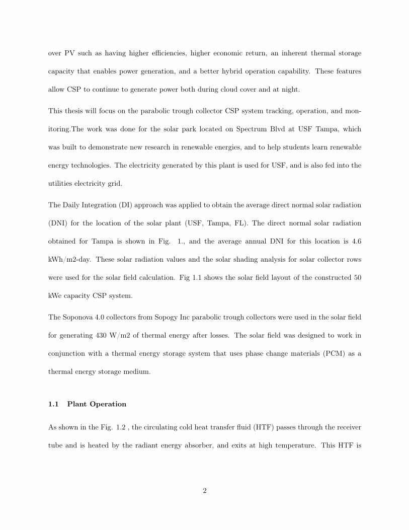
Solar radiation reaches the earth in two formats Direct (Beam) and Diffuse (fig.2.1). Direct radiation

comes in a direct line from the sun with minimal attenuation by the Earth’s atmosphere and other

obstacles. Diffuse radiation is scattered, absorbed and reflected by atmospheric constituents. On

clear days the direct components are high, and the diffuse are low. On cloudy days the total

radiation is low, and most of it has diffuse component. The total or global radiation is the sum

5

of direct, diffuse and reflected radiation (reflected radiation from surface features). Concentrating

solar plant (CSP) can only use direct normal (or) beam radiation (DNI) because diffuse radiation

cannot be effectively focused or concentrated on the collectors. [4]

Figure 2.1: Solar Radiation

2.3 Current CSP Technologies

CSP plants can be classified into two types based on whether the solar collectors concentrate the

sun rays on a focal line or a single focal point (with much higher concentration factors). Focal line

systems include the parabolic troughs, linear fresnel mirrors, and have single-axis tracking systems.

Point focusing systems are the solar dishes and solar tower systems, and include two-axis tracking

systems to follow the sun.

CSP plants can be integrated with heat storage systems to generate power even when the sky is

cloudy or after sunset. For example, during sunny hours, the heat from concentration can be stored

in a high-thermal-capacity fluid, and used upon demand to produce electricity. Thermal storage

6

can significantly improve the capacity factor of CSP plants, as well as their grid integration and

economic competitiveness. To provide the required thermal energy for storage, the solar field (i.e.

mirrors and heat collectors) size of the CSP plant must be oversized with respect to the nominal

electric capacity (MW) of the plant. There is a tradeoff between the incremental cost associated

with thermal storage and increased electricity production. Capacity factor is the number of hours

per year that the plant can produce power. The solar multiple is the ratio of the actual size of

the solar field to the solar field size needed to feed the turbine at nominal design capacity with

maximum solar irradiance (about 1 kW/m2). To cope with thermal losses, plants with no storage

have a solar multiple between 1.1-1.5 while plants with thermal storage may have solar multiples of

3-5.

While CSP plants primarily produce electricity, they also produce high-temperature heat that can

be used for industrial processes, space heating and cooling, and heat-based water desalination

processes. Desalination is particularly important in the sunny and arid regions where CSP plants

are often installed.

2.3.1 Parabolic Trough Systems

The parabolic trough collector (PTC) systems (fig.2.2) consist of a series of mirrors which form the

solar collectors, the combination of collectors (Solar arrays), heat receivers, tracking components,

and their support structures. The parabolic mirrors are formed by coating a sheet of reflective

material into a parabolic shape.This shape concentrates the incident solar radiation onto a central

receiver tube at the focal line of the collector. The arrays of mirrors can be 100m long or more

and with the curved aperture of 5m to 6m. The receiver comprises of the absorber tube which

is usually metal, inside an evacuated glass envelope. The absorber tube is typically coated with

7

Figure 2.2: Parabolic Trough Technology.

stainless steel, with a spectrally selective coating that absorbs the solar irradiation well, but emits

very little infrared radiation. This helps to reduce heat loss and evacuated glass tubes also help to

reduce heat losses. Heat transfer fluid (HTF) is circulated through the absorber tubes where it is

heated to high temperatures, and is then transferred to a steam generator or a heat storage system.

Synthetic oils that are stable up to 400 °C are the heat transfer fluid in most of the parabolic trough

plants. Some of the plants, however, are considering molten salt at 540°C either for heat transfer

and/or as the thermal storage medium, because at high temperatures molten salt can improve the

thermal storage capacity. Single axis tracking mechanism is used in PTC plants to track the solar

arrays on to the sun. PTC ’s are usually aligned North-South and track the sun through East to

West to maximize the collection of sun radiation. [5]

8

2.3.2 Solar Tower Technology

Solar tower systems (fig.2.3) use a number of small mirrors called heliostats. These are tracked in

dual axis to focus direct solar irradiation (DNI) onto a receiver mounted high on a central tower.

The heat receiver can be either a photovoltaic receiver for high concentrated solar radiation for direct

electricity generation (Concentrating Photovoltaics-CPV), or a thermal receiver (CSP) where the

focused radiation is captured and converted into heat. The heat then drives a thermodynamic cycle,

typically a water-steam cycle, to generate electricity. Solar towers can achieve higher temperatures

than parabolic troughs and linear Fresnel systems, because more radiation is concentrated on a

receiver and the heat losses can be minimized. Current solar towers use water/steam, air, or molten

salt to transfer the heat to the heat-exchanger/steam turbine system. Depending on the receiver

design and the working fluid, the upper working temperatures can range from 250°C to as high

as 1000 °C.Temperatures of around 600°C are typical with current molten salt systems.[5] A great

advantage of a solar tower system with a thermal receiver is the possibility to store the heat in

a thermal energy storage and to use the heat at a later time. This thermal energy storage is

significantly lower cost than the battery storage systems used in technologies that directly produce

electricity, such as wind turbines or photovoltaic systems.

Compared to linear concentrating solar power plants such as parabolic trough systems and linear

Fresnel reflectors, solar towers plants can reach significantly higher temperatures from 500 to 1000°C.

Therefore, the turbines can convert the heat into electricity more efficiently, as the efficiency of

turbines increases with the temperature. In addition to power generation, solar towers could also

be used in many applications where high-temperature heat or steam is required. Cost Analysis of

concentrating solar power towers could achieve significant market share in the future. Currently

9

Figure 2.3: Solar Tower Technology (Source [6])

the market is dominated by PTC systems due to lack of commercial experience and, therefore,

deploying solar towers today includes significant technical and financial risks. [5]

2.3.3 Linear Fresnel Collector Systems

Linear Fresnel Collectors (LFC’s) systems (fig.2.4) are similar to PTC’s, but they use a series of

long flat or slightly curved mirrors placed at different angles to reflect the sunlight on either side of

a receiver tube, typically located several meters above these mirrors. They use a single-axis tracking

system to concentrate sunlight on the fixed receiver. The receiver consists of a long, selectively-

10

Figure 2.4: Linear Fresnel Collector Systems

coated absorber tube. These require a secondary reflector to refocus the rays missing the tube,

or several parallel tubes forming a multi-tube receiver that is wide enough to capture most of the

focused sunlight without a secondary reflector. The main advantages of LFC CSP systems compared

to PTC CSP systems are cheaper flat glass mirrors, less steel and concrete, lighter support structure ,

easy assembly process, lower wind loads, low optical losses, less mirror-glass breakage. However, the

optical efficiency of LFC systems is lower than that of PTC plants due to the geometric properties

of LFC’s. The main problem is that the cosine losses are high compared to PTC receivers, as these

have fixed receivers.[5]

11

2.3.4 Stirlings Dish Technology

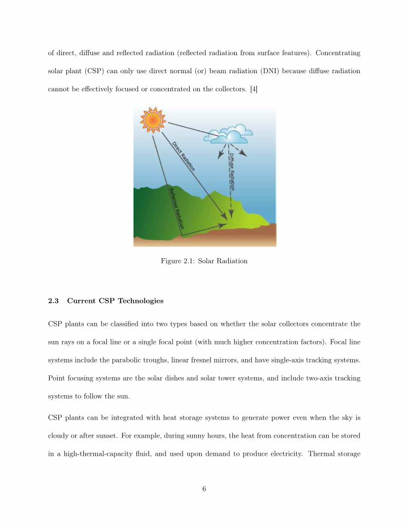
The Stirling dish system, as shown in fig. 2.5, consists of a parabolic dish-shaped concentrator (like

a satellite dish) which reflects direct solar irradiation (DNI) onto a receiver located at the focal

point of the dish. The receiver can be a Stirling engine (dish/ engine systems) or a micro-turbine

combination with a generator unit, located at the focus of the dish. This system needs to be tracked

in two axes, but the high energy concentration onto a single point can yield very high temperatures.

The advantage of Stirling dish CSP technologies is that the location of the generator is generally

located in the receiver of each dish, thus reducing heat loss. Stirling dish systems can achieve higher

efficiencies than all other types of CSP systems, uses dry cooling (Air Cooling), and do not need

water cooling systems or cooling towers. CSP technology has the capability to provide electricity in

water-constrained regions. Unlike PTC, LFC and solar towers, these systems can be implemented

on slopes and uneven terrains. In spite of these advantages, the sterling dish CSP systems could

be economically viable options in many regions, though the levelised cost of electricity (LCOE) is

likely to be higher than other CSP technologies. However, the dish systems can’t easily use storage.

Also, they are still in demonstration stage. But with their high degree of scalability and small size,

stirling dish systems will be an alternative to solar photovoltaics in arid regions.[5]

2.4 Conclusion

The four CSP technologies discussed above work on the same principle but differ significantly from

one another, not only in technical and economic aspects, but also in their reliability, maturity

and operational experience in utility-scale. Most CSP projects currently under construction or

development are based on parabolic trough technology, as it is the most mature technology and

12

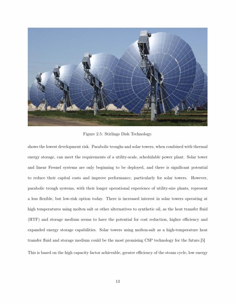
Figure 2.5: Stirlings Dish Technology.

shows the lowest development risk. Parabolic troughs and solar towers, when combined with thermal

energy storage, can meet the requirements of a utility-scale, schedulable power plant. Solar tower

and linear Fresnel systems are only beginning to be deployed, and there is significant potential

to reduce their capital costs and improve performance, particularly for solar towers. However,

parabolic trough systems, with their longer operational experience of utility-size plants, represent

a less flexible, but low-risk option today. There is increased interest in solar towers operating at

high temperatures using molten salt or other alternatives to synthetic oil, as the heat transfer fluid

(HTF) and storage medium seems to have the potential for cost reduction, higher efficiency and

expanded energy storage capabilities. Solar towers using molten-salt as a high-temperature heat

transfer fluid and storage medium could be the most promising CSP technology for the future.[5]

This is based on the high capacity factor achievable, greater efficiency of the steam cycle, low energy

13

storage costs, and firm output capability. While the levelised cost of electricity (LCOE) of parabolic

trough systems does not tend to decline with higher capacity factors, the LCOE of solar towers tends

to decrease as the capacity factor increases. This is mainly because of significantly lower specific

cost of the molten-salt energy storage in solar power tower plants. CSP technologies offer a great

opportunity for local manufacturing, which can stimulate local economic development, including

job creation. [5]

14

CHAPTER 3 : TRACKING SYSTEM DESIGN

3.1 Introduction

Solar tracking can be used in wide range of solar applications including concentrated solar power

generation, steam generation, desalination, water purification, electricity generation, industrial pro-

cess heat, thermal heat storage, food dryers and water pumping. An automated sun tracking system

maximizes the energy output of solar power plants. In these type of renewable energy systems, the

solar positioning systems or solar angle calculators are used in tracking the PV panels, parabolic

mirrors, Dishes , heliostats etc. [7]

An auto tracking solar system uses solar position algorithm which points the solar reflector exactly

at the sun and locks on the sun’s position to track the sun across the sky throughout the day.

Automatic solar tracking can be either single-axis sun solar tracking or dual-axis sun tracking. It

depends on the employed solar system, PV (Photovoltaic) system dual axis tracking isn’t as much

difficult as in the case of Parabolic trough system (CSP), because the weight of the modules of PV

are fewer compared to parabolic trough system.

15

Many open-source sun tracking algorithms and source-code for solar tracking programs are freely

available to download on the internet today. The programs used by these solar position calculators

and solar simulation softwares use machine program code for the controllers, which are software

programmed into Programmable Logic Controllers (PLC), Micro controllers, Arduino processor, or

PIC processor etc. GUI libraries with graphical control elements are also available to design the

graphical user interface (GUI), which can be used to monitor the entire solar power plant.

3.1.1 Module Tracking

Optical encoders generally can be employed in the closed-loop control systems in order to activate

the drive mechanisms and achieve the precise movement of the solar modules. This can pin-point

exact solar position in the sky. The feedback signals generated by the sensors inform the controller

whether the mirror’s or PV’s are locked onto the sun.

Optical sensors such as photodiodes, photo resistors, light dependent resistors (LDR), or encoders

are used as optical accuracy feedback devices. But, any closed loop solar tracking system that uses

only optical sensor devices is easily affected by environmental factors such as clouds and weather

conditions. Moreover these systems are expensive.

There are other angle measuring sensors that can be used in solar tracking applications, such as

tilt sensors, accelerometers, gyroscope, magnetometers, and inclinometers. These are typically less

expensive, and use low-power to detect orientation or inclination on the elevation axis. These can

simply stick/mount anywhere, are sealed and do not wear out, so they have limited moving parts.

16

3.2 Tracker Design

Concentrating solar plant (CSP) can only use direct normal (or) beam radiation (DNI), because

diffuse radiation cannot be effectively focused or concentrated on the collectors. CSP Systems need,

to track the sun throughout the day to concentrate the beam radiation on the absorber tube.

3.2.1 Calculating the Sun Path and Angle

With increase of the use solar energy, there is a need for accuracy solar position. Many algorithms

and methods were published regarding calculating the solar position with uncertainties of 0.01°for

solar zenith and azimuth angle calculations, Most of these are only valid for a specific number

of years. But the technical report " Solar position for Solar radiation application " published

by National Renewable Energy Laboratory (NREL) has Solar Position Algorithm (SPA) which

calculates the solar zenith and azimuth angle with uncertainty of Âś 0.0003 °in the period -2000

-6000 based on the date, time, and location on Earth. [8] This Algorithm was used in the tracking

system design to calculate the sun angle. The following are the list of some important parameters

that are used in the calculation of sun position in the SPA Algorithm Latitude: the angle north or

south of the equator Longitude, the east-west position relative to the Greenwich Solar Declination,

the angle between the earth and sun line through their centers and the plane through the equator, it

varies between -23.45 °on December 21 to +23.45 °on June 21 Surface azimuth angle, the deviation

of the direction of the slope to the local meridian Solar azimuth angle,the angle of the sun to local

meridian or surface azimuth, the Solar-vector elevation from observer solar Zenith angle and the

angle between the place to sun line and the vertical at the place. All the above parameters were

calculated in degrees. The day light adjustment of the present location has to be used to provide the

17

actual date and time of location. The actual date and time is an important input to the algorithm,

which needs to be exact.

The algorithm was programmed in Structured Control Language (SCL) in Siemens TIA Portal V13

and then was converted to Functional Block, which represents a detailed view of inputs to the al-

gorithm, and outputs from the algorithm.

Figure 3.1: Functional Block of Solar Position Algorithm

18

3.2.2 Rotating the Collectors to the Sun Angle

The next major task is to rotate the collectors to this angle. To achieve this, a number of hardware

components are employed.

3.2.3 Components Used

1. Programmable Logic Controller (PLC)

The Main Tracking component of the design is the Programmable Logic Controller (PLC).

PLC is a computer that continuously monitors the inputs and processes the outputs based on

the algorithm or program coded into its memory. With increase in demand for automation,

many PLC’s are available in the market and Siemens controllers are well known for their user-

friendliness, different programming languages, durability, shorter processing times with faster

communication, and data access for increased productivity. They also have perfect security

integrated procedures for the device protection, and secure communication between modules.

There are many types of Programmable logic controllers in Siemens for different range of

automation tasks. Among all these controllers S7 1200 1214 AC/DC/RLY CPU was selected

based on the tracking components and inputs, Outputs used.

This PLC supports 14 Digital Inputs,and 10 Digital Relay outputs. The designed control

system needs 7 more Relay outputs to process the tracking of 14 solar arrays in the system.

To accomplish this, the Signal module SM 1222 RLY was added to the design. To communicate

with the Inclinometers of the tracking system, the communication module CM 1241 RS 232

was added to the controller. The table 3.1 lists Input & Output tags used in the PLC Program.

2. Inclinometers

19

Figure 3.2: S7 1200 1214 CPU AC/DC/RLY

Figure 3.3: CM 1241 RS 232 Module

The angle of the collectors is a crucial piece of information that needs to be accurate to achieve

perfect tracking for the collectors. Inclinometers were used to determine the present angle of

20

Table 3.1: Input and Outputs Tags for the PLC Program

I/O Tag name Logical Address

InputsTRACK %I0.1

ROWS DEFOCUS %I0.2

OutputsRow1 %QO.0Row2 %Q0.1Row3 %Q0.2Row4 %Q0.3Row5 %Q0.4Row6 %Q0.5Row7 %Q0.6Row8 %Q0.7Row9 %Q1.0Row10 %Q1.1Row11 %Q9.0Row12 %Q9.1Row13 %Q9.2Row14 %Q9.3

Motion Ignition %Q9.4Speed %Q9.5F/R %Q9.6

Figure 3.4: SM 1222 RLY Module

the collectors. Inclinometers measure tilt of an object with respect to gravity. US Digital

T7-1-CAN inclinomters are used in the present tracking system, as this is specially designed

for applications like solar tracking, construction equipment, and warehouse automation etc.

21

This T7 networked absolute inclinometer calculates angles over a full 360 °range in a single

axis and is designed to use in dirty environments. The T7 calculates inclination by sensing

the acceleration from solid state accelerometers integrated into a monolithic chip. Gravity,

centrifugal forces, and linear speed changes are all forms of acceleration. The T7 will report

the mathematically calculated tilt angle based on all sensed accelerations.

The T7 is compatible with several interfaces and a variety of industrial protocols. The physical

interface can be RS232, RS485 orUS Digital’s CAN (Controller Area Network). The protocol

can be either US Digital’s serial protocol or Modbus RTU. The interface was selected based

on the distance of cable that the type can support. [1]

The RS232 version can support a single T7 with up to 100ft of cable, but the RS485 and

US Digital CAN (Controller Area Network) version can be used to connect multiple T7’s in

single network of longer cable lengths of up to 250ft and1000ft respectively. US Digital CAN

network was selected for this design, as it has 14 rows of collectors with cable length up to

300ft. [1]

Figure 3.5: T7-1-CAN Inclinometer (Adapted from [1])

22

3. Command translator

The Programmable Logic controller (PLC) needs to read the angle from the Inclinometer to

execute the programmed operations. The PLC supports the RS232 and RS485 Interface to

communicate with it, and the Inclinometer runs on Controller Area Network (CAN) interface

to communicate with it. A Signal translator is needed to establish communication between

PLC and Inclinometer.

Figure 3.6: CANA 232 Adapter (Adapted from [2])

The CANA-232 adapter from US Digital allows a host PC or PLC to communicate with a

network of up to 64 CAN interface version of T7. It serves as command translator between

the Serial Ports RS232 or RS 485 and CAN bus is used by the T7 inclinometer network.

A network needs to be established using daisy chain configuration through which the controller

communicates with all the inclinometers installed in the tracking system [2]

There are different daisy chain network configurations for CANA-232 and T7-1-CAN Incli-

nometer.

23

(a) Single Line Configuration

For this daisy chain configuration (fig.3.7) there are two ends. The CAN adapter is on

one end, so the built in termination resistor has to be jumpered and the other end and

has a T7 Inclinometer which needs to be installed with a cable having the termination

resistor to form a network.[2]

Figure 3.7: Single Line Configuration of Inclinometer Network (Adapted from [2])

(b) Parallel Line Configuration

In this type of daisy chain configuration (fig.3.8), both the ends have Inclinometers

that need to be installed with the terminating resistor cables, but the jumper on the

terminating resistance of CANA 232 should be removed to form a network.[2]

4. Speed Controls

The permanent magnetic DC gear motor used in the tracking system needs to have a speed

controller to achieve accuracy in tracking. To stop the motor at a certain angle it’s speed needs

to decelerate well before. DC basic speed control, which employs pulse width modulation for

precise speed control, was used in this design.

24

Figure 3.8: Parallel Line Configuration of Inclinometer Network(Adapted from [2])

Figure 3.9: Speed Controller of Motor

The speed of the motor can be controlled using 0-5VDC remote signal or manually by using

10 kÎľ speed potentiometer.

25

5. Limit Switches

Due to the mechanical design of the collector assembly in the present solar power plant, col-

lectors cannot be allowed to rotate 360 degrees, Moreover we do not need to track the sun

throughout 0-360 degrees as one revolution of sun comprises both North and South hemi-

spheres. It is optimum to limit the tracking of collectors to a certain angle.

The limit switch (fig.3.10) is tied to the control circuit of the motor, so that the forward

motion of the motor is allowed until the collectors touch the limit switch. When the collectors

make a contact with the limit switch, only reverse motion of the motors is allowed. Such a

design was used to limit the tracking angle of the system.

6. Motor Motion Control

The motor rotation needs to be in both forward and reverse directions to do the tracking. The

reverse direction of the motor can be achieved by simply switching the polarities of the power

supply. A double pole double throw relay was used to switch the polarities of the motor.

The DPDT relay(fig.3.11) has eight terminals. The first two on the left are to energize the

relay. The Right part of the relay contains two normally open, two normally closed and two

common terminals. During the normal state the common and normally closed terminals will

be in contact with each other. When the relay energizes the normally closed contact breaks

with the common contact and makes contact with normally open contact. The terminals of

the motor can be swapped using the above logic and thus we can control the motion of the

motor forward and in reverse.

26

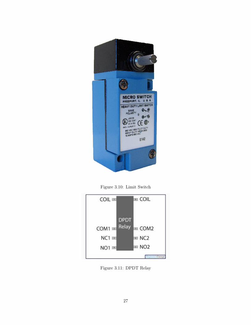
Figure 3.10: Limit Switch

Figure 3.11: DPDT Relay

27

3.2.4 Tracker Flowchart

As shown in the figure 3.12, the tracking process starts when the programmable logic controller

(PLC) gets the tracking on signal. Then, it selects the row that it needs to rotate (usually row 1

Figure 3.12: Tracker Block Diagram

during the start of the day). Based on the present angle of the row and the calculated the angle of

28

the it decides the motion (forward or reverse) that needs to be executed. It also looks for the set

points in the program that changes the speed of the motors. If the angle calculated is within the

set points, it rotates the motor with slow speed until it reaches the target angle. After rotating that

row to that angle, it selects another row and repeats the same cycle. This process continues until

the tracking signal stays on for the PLC. But as soon as it sees the Tracking signal go off, the PLC

rotates all the rows back to stow position (20 degrees). This saves the collectors from high speed

winds during non-tracking state of the plant. The 20 degrees of stow position was selected because

it was shown that the collectors can exhibit maximum wind resistance at this angle.

29

CHAPTER 4 : POWER PLANT OPERATION AND MONITORING

Operation of a solar power plant is an important aspect to optimize the levelised cost of electricity

(LCOE), and the safety of the plant/the workers in the plant, as they use high temperatures

and several machines which are harmful. The main components which need to be monitored and

maintained during the operation are temperature measuring devices, flow meters, pumps, motors,

valves, solar radiation measuring sensors, and the internal components of the power block.

4.1 Temperature Sensors

The most widely measured physical parameter is temperature. Whether in process industry ap-

plications, chemical Plants, buildings etc., accurate temperature measurement is a critical part in

their operation. There are many different types of sensors available to measure temperature. The

three most common devices are resistance temperature detectors (RTD’s), thermocouples (TCs),

and thermistors. Each of them have specific operating parameters that may make it a better choice

for some applications than others. [7]

4.1.1 Thermocouple

The most commonly used temperature sensor is the thermocouple or TC. The key reasons are

that thermocouples are low cost, extremely robust, can be run long distances,and are self-sourced

(require no external power supply), Additionally, there are many types of thermocouples available

to cover a wide range of temperatures. But Thermocouples are nonlinear and require cold-junction

30

compensation (CJC) for linearization. Also, the voltage signals are low requiring careful techniques

to eliminate noise and drift in low-voltage environments. Accuracies are typically in the range of

1-3%.

4.1.2 RTD

One of the most accurate temperature sensors is a resistance temperature detector, or RTD. In an

RTD, the resistance of the device is proportional to temperature. The most common material for

RTD’s is platinum, but some of them use nickel and copper as well. RTD’s have a wide range of

temperature measurement. Depending on how they are constructed, they can measure temperatures

in the range of -270 °C to + 850 °C. RTD’s have long term stability compared to Thermocouple

and Thermistor. [7]

4.1.3 Thermistor

The thermistor offers higher sensitivity than RTDs, meaning that the thermistor resistance will

change much more in response to temperature changes than an RTD. However, non-linear properties

of thermistors require linearization. They also have a limited temperature range and are not as

rugged as TCs or RTDs. Because thermistors are semiconductors, they are more likely to have

de-calibration issues at high temperature. [7]

Table 4.1: Temperature Sensors Characteristics

Thermocouple RTD ThermistorRange -200 °C to 2000 °C -250°C to 850 °C -100 °C to 300 °C

Accuracy 1 °C 0.03 °C 0.1 °CCost Low High Low to ModerateLong Term Stability Low High Medium

31

So RTD’s were selected as temperature sensing devices for this power plant by considering their

long term stability and temperature range.

Figure 4.1: Resistance Temperature Detector Schematic

But the temperature of output of the RTD is 4-20 mV and the controller uses either 4-20 mA or

0-10 V for Analog input and outputs. There is a need of converter which takes 4-20 mV and produce

4-20 mA signal.

Figure 4.2: TX92G 4 Temperature Transmitter

The above temperature transmitter (TX92G-4) from Omega takes the three wire RTD sources and

converts the output of 4-20 mA at the negative terminal.

32

4.2 Flow-Loop Hardware

4.2.1 Flow Meters

Measuring the flow of liquids is a critical need in many industrial plants. To run a solar power plant

at maximum efficiency, operators and engineers need to have an accurate knowledge of heat transfer

fluid (HTF) flow rates through the solar fields. The reliability of the flow meters is also important,

because failures could lead to plant outages.

Flow Meters measure the velocity of flowing liquids by counting the frequency at which the blades

of a rotating turbine pass a fixed electrode. Circuitry within the flow meter electronics enclosure

then converts the rotational rate to digital and/or analog signals.

Figure 4.3: Flow Meter Schematic

As shown in the fig. 4.3 the flow meter generates the 4-20 mA signal corresponding to the flow rate.

The mathematical scaling of the signal can be calculated using this formula.

Current output = (measured current in mA - 4) X Full Scale Analog Flow Rate Gallons per minute

(GPM) 16

33

4.2.2 Pumps

The heat transfer fluid needs to flow with certain rate through the absorb tubes so that they can

absorb the radiation on the absorber tube. To achieve this flow rate and pressures, we need to use

the pumps. Care must be taken in the solar field design so that all the solar arrays in the collectors

have same flow rate. If they have different flow rates, it leads to inefficiency in heat transfer to the

fluid.

4.2.3 Valves

The Heat transfer fluid needs to be circulated within in the solar field for a certain period of time

to get heated to set temperatures before entering in to the power block for steam cycle. We need

to stop the HTF entering in to the power block during this process. A valve can be used here to

activate or allow the flow into the power block when it is not energized. When it is energized, it

blocks the fluid entering into the power block. The flow rates into the power block can also be

controlled by opening the valve up to certain positions.

Solenoid valves are used when fluid flow has to be controlled. Solenoid valves are control units

which, when electrically energized or de-energized, either cut off or permit fluid flow. The actuator

is an electromagnet. When the valve is energized, a magnetic field builds up which pulls a plunger

or pivoted armature against the action of a spring. When de-energized, the plunger or pivoted

armature is returned to its original position by the action of the spring.

34

Figure 4.4: Plant Operation and Maintenance Flowchart

4.3 Operation and Monitoring

As shown in the fig.4.4, the concentrated solar power plant at USF, Tampa operation begins when

the direct normal irradiation (DNI) goes beyond the set point, so the controller starts tracking the

35

collectors on to the sun. The Heat transfer fluid (HTF) is pumped through the collector receiver

tubes to absorb the heat energy from the reflected radiation on the receiver tubes. But the HTF

cannot be allowed to enter into the power block until it reaches certain temperatures, because with

low temperatures it’s not possible to achieve the required thermal energy to run the generator.

The HTF will be circulated in the solar arrays until it reaches the set temperature of the plant

design. After reaching that temperatures , it is very important to check whether the power block is

ready to take the heat or not, because the power block consists of components like heat exchanger,

evaporator, generator, pumps, condenser etc. These elements deal with high temperatures and

pressures. Care must be taken before adding heat to the power block. The designed control system

of the power block needs to monitor all these parameters, and provide feedback to allow the heat.

After successful feedback from the power block control system, the HTF is injected in to the power

cycle where its heat will be exchanged in the heat exchanger, and ejected back into the solar arrays

to reheat.

When DNI is higher than the designed capacity of the plant, there is chance that the HTF can go

over the maximum temperature that can withstand without decomposing, so appropriate care must

be taken to keep the HTF in the designed temperatures. If the HTF beyond than the set point, it

must be stopped to absorb the heat, which can be done by defocusing the solar arrays to a certain

angle (typically 15 °). The HTF will again be allowed into the power block when it comes down to

the set temperature.

Under any conditions, if the plant is going to shut down its operation, the solar arrays needs to

be protected from the environmental factors and weather conditions. Solar field operation becomes

quite challenging during times of high wind velocities. Mirrors can easily be affected by high

36

wind forces. To protect the plant mirrors, they need to be rotated at a wind-safe position when

wind speeds exceed the designed wind loads on collectors. Longer operation hours without a total

solar field stow may be possible if a high-wind operating strategy is adopted, which simultaneously

protects the field from damage and allows most of the field to continue to operate.

4.3.1 Field Monitoring

Even though the developed control system has the ability to control and automate the plant opera-

tions, the maintenance unit and operator needs to monitor several parameters and do maintenance

to clear the issues. The field data monitoring system is indispensable for these type of plants. How-

ever, there are many software technologies available in the market, like OPC servers, and SCADA,

which gives you real time data of the plants. Automated Logic’s WebCTRL is a state of the art au-

tomation system software package that gives the ability to the user to program, monitor, visualize,

configure and operate the automation system in one terminal. It also offers intuitive user interface

and powerful control features. These have potential to give the operator access to the plant’s real

time data from anywhere in the world through a number of devices - including desktop computers,

laptop computers and tablets and cell phones. This software was used to design the plant SCADA

system. [9]

37

Figure 4.5: Power Plant Operation Program

Figure 4.6: SCADA VIEW

38

CHAPTER 5 : CONCLUSION

Precise tracking, operation and maintenance are the key factors for the economical growth of solar

power plants. The generation potential of a solar CSP plant is largely determined by the location

DNI. Tracking the sun provides a significantly greater energy yield for a given DNI than a fixed

surface, so the performance of the solar field is strongly influenced by the ability of the designed

tracking system to focus the solar beam on the solar arrays. There are many ways to track the sun

depending upon the size and location of the power plant. Also, the mirrors should also be frequently

cleaned because the dust particles accumulated on them will degrade their reflectivity.

This thesis developed a cost-effective methodology for designing of a tracking and operating system

for parabolic trough solar power plants without thermal storage. The methodology is based on the

individual analysis of different components and subsequent integration of these components into the

design. This design was validated by installing the parabolic trough concentrated solar power plant

at University of South Florida, Tampa. This design is suitable for all single axis tracking systems

Plants with higher DNI, good tracking, operation, and maintenance will yield more energy, allow

greater electricity generation, and have a correspondingly lower LCOE. So the relationship between

DNI, energy output, and the LCOE of electricity is strong.

39

REFERENCES

[1] US DIGITAL. T7 networked absolute inclinometer, 2015.

[2] US DIGITAL. Can to serial port adapter, 2015.

[3] U.S. Energy Information Administration (EIA). Annual energy outlook 2015 (aeo 2015).

[4] D Yogi Goswami, Frank Kreith, and Jan F Kreider. Principles of solar engineering. CRC Press,

2000.

[5] IRENA. Renewable energy technologies: Cost analysis series. 1.

[6] Arvind. Solar tower systems. http://projectfinancetoday.com/solar-tower-systems/, Dec 2012.

[7] Robert Dobson and Gerro Prinsloo. Automatic solar- tracking, sun-tracking systems,solar track-

ers and automatic sun tracker systems.

[8] Ibrahim Reda and Afshin Andreas. Solar position algorithm for solar radiation applications.

Solar energy, 76(5):577–589, 2004.

[9] Automated Logic. Webctrl,powerful and intuitive front end for building control, 2015.

40

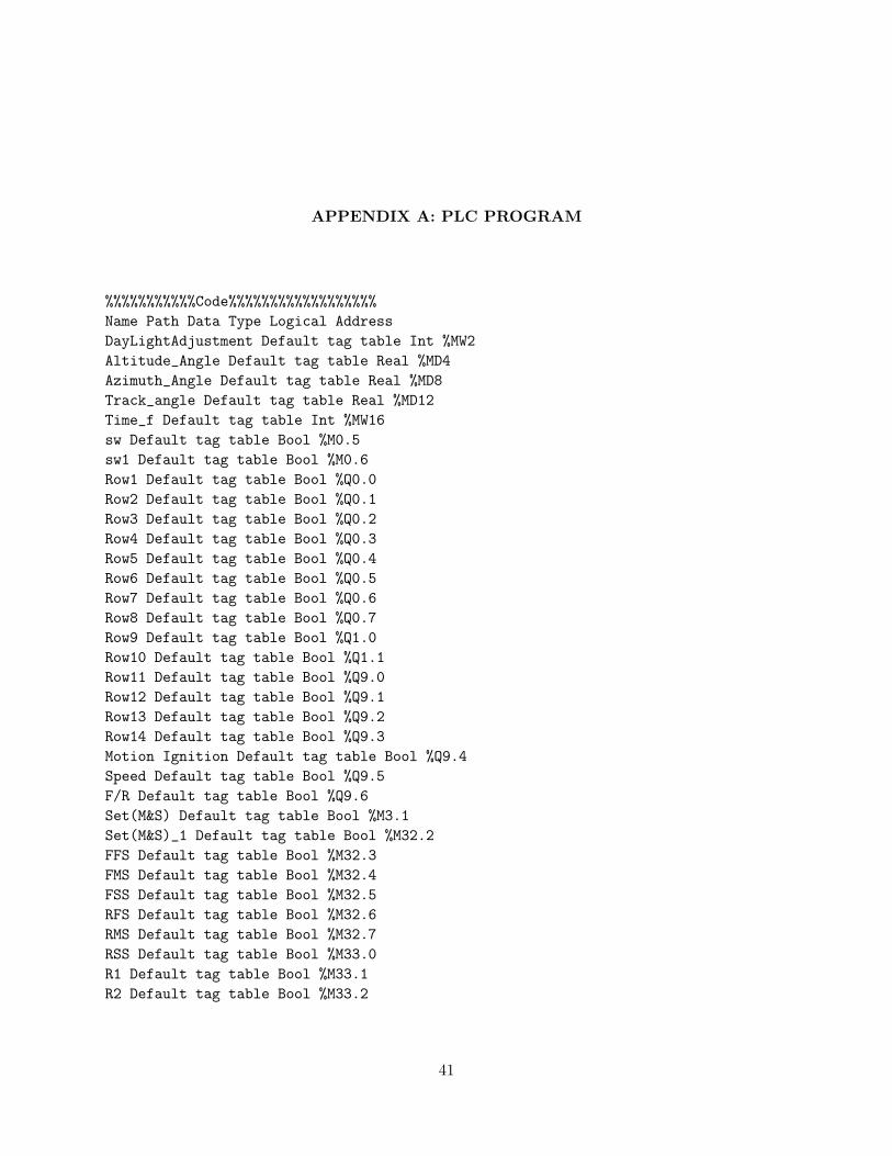
APPENDIX A: PLC PROGRAM

%%%%%%%%%%%Code%%%%%%%%%%%%%%%%%%Name Path Data Type Logical AddressDayLightAdjustment Default tag table Int %MW2Altitude_Angle Default tag table Real %MD4Azimuth_Angle Default tag table Real %MD8Track_angle Default tag table Real %MD12Time_f Default tag table Int %MW16sw Default tag table Bool %M0.5sw1 Default tag table Bool %M0.6Row1 Default tag table Bool %Q0.0Row2 Default tag table Bool %Q0.1Row3 Default tag table Bool %Q0.2Row4 Default tag table Bool %Q0.3Row5 Default tag table Bool %Q0.4Row6 Default tag table Bool %Q0.5Row7 Default tag table Bool %Q0.6Row8 Default tag table Bool %Q0.7Row9 Default tag table Bool %Q1.0Row10 Default tag table Bool %Q1.1Row11 Default tag table Bool %Q9.0Row12 Default tag table Bool %Q9.1Row13 Default tag table Bool %Q9.2Row14 Default tag table Bool %Q9.3Motion Ignition Default tag table Bool %Q9.4Speed Default tag table Bool %Q9.5F/R Default tag table Bool %Q9.6Set(M&S) Default tag table Bool %M3.1Set(M&S)_1 Default tag table Bool %M32.2FFS Default tag table Bool %M32.3FMS Default tag table Bool %M32.4FSS Default tag table Bool %M32.5RFS Default tag table Bool %M32.6RMS Default tag table Bool %M32.7RSS Default tag table Bool %M33.0R1 Default tag table Bool %M33.1R2 Default tag table Bool %M33.2

41

R3 Default tag table Bool %M33.3R4 Default tag table Bool %M33.4R5 Default tag table Bool %M33.5R6 Default tag table Bool %M33.6R7 Default tag table Bool %M33.7R8 Default tag table Bool %M34.0R9 Default tag table Bool %M34.1R10 Default tag table Bool %M34.2R11 Default tag table Bool %M34.3R12 Default tag table Bool %M34.4R13 Default tag table Bool %M34.5R14 Default tag table Bool %M34.6STOP Default tag table Bool %M35.1Rowselected Default tag table Int %MW35Row Track angle Default tag table Real %MD38R1SAVE Default tag table Bool %M42.1condition_2 Default tag table Bool %M42.2Set Angle Default tag table Real %MD42Day Status Default tag table Bool %M46.0DEFOCUS Default tag table Bool %M46.1Present Row Offset Default tag table Real %MD48Auto Default tag table Bool %M52.0Manual Default tag table Bool %M52.1Offset Default tag table Bool %M52.2ROW 1 DESELECT Default tag table Bool %M52.3ROW 2 DESELECT Default tag table Bool %M52.4ROW 3 DESELECT Default tag table Bool %M52.5ROW 4 DESELECT Default tag table Bool %M52.6ROW 5 DESELECT Default tag table Bool %M52.7ROW 6 DESELECT Default tag table Bool %M53.0ROW 7 DESELECT Default tag table Bool %M53.1ROW 8 DESELECT Default tag table Bool %M53.2ROW 9 DESELECT Default tag table Bool %M53.3ROW 10 DESELECT Default tag table Bool %M53.4ROW 11 DESELECT Default tag table Bool %M53.5ROW 12 DESELECT Default tag table Bool %M53.6ROW 13 DESELECT Default tag table Bool %M53.7ROW 14 DESELECT Default tag table Bool %M54.0TRACK Default tag table Bool %I0.1ROWS DEFOCUS Default tag table Bool %I0.2PLC TRACK Default tag table Bool %M54.1PLC TRACK OFF Default tag table Bool %M54.2INCLINOMETER COM Default tag table Bool %M54.3

42

////Solar Tracking system Program (Structured Text)//

IF "TRACK" = 1 THEN// Track Signal from FLEX HOUSE controller

"PLC TRACK" := 1;"INCLINOMETER COM" := 0;// Inclinometer Communications Starts"PLC TRACK OFF" := 0;

IF "ROWS DEFOCUS" = 1 THEN// ROWS DEFOCUS Signal from FLEX HOUSE controller

"DEFOCUS" := 1;ELSE

"DEFOCUS" := 0;END_IF;

ELSIF "TRACK" = 0 THEN"Day Status" := 0;

// TO START the STOW POSITIONING from ROW 1 //

IF "PLC TRACK OFF" = 0 THEN"Data_block_1"."Row Selected" := 1;"PLC TRACK OFF" := 1;

END_IF;

// TO START the STOW POSITIONING from ROW 1 //

END_IF;

// This STOPS the Inclinometer communicationsafter we change from Manual to AUTO MODEduring STOW Position //

IF "Auto" = 0 AND "PLC TRACK" = 0 THEN

"INCLINOMETER COM" := 1;

END_IF;

// This STOPS the Inclinometercommunications after we changefrom Manual to AUTO MODE during STOW Position //

43

IF "PLC TRACK" = 1 THEN // TO stop the execution of theAUTO TRACKING program afterbringing the rows to stow position

IF "Auto" = 0 THEN

// This Resets the Timer forAuto Tracking INclinometerFault Checking Control and its TAGS//IF "IEC_Timer_0_DB_11".ET >= T#1000ms THEN

RESET_TIMER("IEC_Timer_0_DB_11");"Data_block_1"."Auto Error" := 0;"Data_block_1"."Auto Error Check" := 0;

END_IF;// This Resets the Timer for Auto TrackingINclinometer Fault Checking Control and its TAGS//

////Track Angle Declaration and Inclinometer setting//

////Motion Commands to Speed ControlBoard throughActivating Relays//

// Delay to ensure the Inclinometer Communications//"Data_block_1"."Auto Start" := 1;"IEC_Timer_0_DB_9".TON(IN := "Data_block_1"."Auto Start",

PT := T#1S,Q => "Data_block_1"."Auto Start SC");

// Delay to ensure theInclinometer Communications//

// Delay for safe Row operation//"Data_block_1"."Row Delay Timer" := 1;"IEC_Timer_0_DB_10".TON(IN := "Data_block_1"."Row Delay Timer",

PT := T#1.5S,

44

Q => "Data_block_1"."Row Delay");

// Delay for safe Row operation//

IF "Data_block_1"."Auto Start SC" = 1 THEN

IF "Set Angle" > 5 THEN"Motion Ignition" := 1;"Speed" := 1;"F/R" := 0;

ELSIF "Set Angle" <= 5AND "Set Angle" > 0.2 THEN

"Motion Ignition" := 1;"Speed" := 0;"F/R" := 0;

ELSIF "Set Angle" <= -5 THEN"Motion Ignition" := 1;"Speed" := 1;"F/R" := 1;

ELSIF "Set Angle" <= -0.3AND "Set Angle" > -5 THEN


ELSIF "Set Angle" <= 0.3AND "Set Angle" > -0.3 THEN

"Motion Ignition" := 0;"Speed" := 0;"F/R" := 0;IF "Data_block_1"."Row Selected" = 1 THEN

"Data_block_1"."Row Selected" := 2;"Data_block_1"."Row Delay Timer" := 0;"Data_block_1"."Row Delay" := 0;"Data_block_1"."Auto Start SC" := 0;"Data_block_1"."Auto Start" := 0;RESET_TIMER("IEC_Timer_0_DB_10");RESET_TIMER("IEC_Timer_0_DB_9");

ELSIF "Data_block_1"."Row Selected" = 2 THEN"Data_block_1"."Row Selected" := 3;

45

"Data_block_1"."Row Delay Timer" := 0;"Data_block_1"."Row Delay" := 0;"Data_block_1"."Auto Start SC" := 0;"Data_block_1"."Auto Start" := 0;RESET_TIMER("IEC_Timer_0_DB_10");RESET_TIMER("IEC_Timer_0_DB_9");

ELSIF "Data_block_1"."Row Selected" = 3 THEN"Data_block_1"."Row Selected" := 4;"Data_block_1"."Row Delay Timer" := 0;"Data_block_1"."Row Delay" := 0;"Data_block_1"."Auto Start SC" := 0;"Data_block_1"."Auto Start" := 0;RESET_TIMER("IEC_Timer_0_DB_10");RESET_TIMER("IEC_Timer_0_DB_9");




ELSIF "Data_block_1"."Row Selected" = 7 THEN

46

"Data_block_1"."Row Selected" := 8;"Data_block_1"."Row Delay Timer" := 0;"Data_block_1"."Row Delay" := 0;"Data_block_1"."Auto Start SC" := 0;"Data_block_1"."Auto Start" := 0;RESET_TIMER("IEC_Timer_0_DB_10");RESET_TIMER("IEC_Timer_0_DB_9");



ELSIF "Data_block_1"."Row Selected" = 10 THEN"Data_block_1"."Row Selected" := 11;"Data_block_1"."Row Delay Timer" := 0;"Data_block_1"."Row Delay" := 0;"Data_block_1"."Auto Start SC" := 0;"Data_block_1"."Auto Start" := 0;RESET_TIMER("IEC_Timer_0_DB_9");



47




// TO stop theexecution of the program after bringing the rows to stowposition//

IF "Day Status" = 0 THEN"PLC TRACK" := 0;"Data_block_1"."Row Selected HMI" := 0;"PLC TRACK OFF" := 0;"INCLINOMETER COM" := 1; /

"Data_block_1".Angle := 0;END_IF;

END_IF;

END_IF;END_IF;

48

END_IF;

////Motion Commands toSpeed Control Board throughActivating Relays//

//Activating the rows//IF "Data_block_1"."Row Selected" = 1AND "Data_block_1"."Row Delay" = 1 THEN

"Row2" := 0;"Row3" := 0;"Row4" := 0;"Row5" := 0;"Row6" := 0;"Row7" := 0;"Row8" := 0;"Row9" := 0;"Row10" := 0;"Row11" := 0;"Row12" := 0;"Row13" := 0;"Row14" := 0;"Row1" := 1;

ELSIF "Data_block_1"."Row Selected" = 2 AND"Data_block_1"."Row Delay" = 1 THEN



"Row1" := 0;

49

"Row2" := 0;"Row4" := 0;"Row5" := 0;"Row6" := 0;"Row7" := 0;"Row8" := 0;"Row9" := 0;"Row10" := 0;"Row11" := 0;"Row12" := 0;"Row13" := 0;"Row14" := 0;"Row3" := 1;





50



ELSIF "Data_block_1"."Row Selected" = 7 THEN"Row1" := 0;"Row2" := 0;"Row3" := 0;"Row4" := 0;"Row5" := 0;"Row6" := 0;"Row8" := 0;"Row9" := 0;"Row10" := 0;"Row11" := 0;"Row12" := 0;"Row13" := 0;"Row14" := 0;"Row7" := 1;


"Row1" := 0;"Row2" := 0;"Row3" := 0;"Row4" := 0;"Row5" := 0;"Row6" := 0;"Row7" := 0;"Row9" := 0;"Row10" := 0;"Row11" := 0;"Row12" := 0;"Row13" := 0;

51

"Row14" := 0;"Row8" := 1;





"Row1" := 0;"Row2" := 0;"Row3" := 0;"Row4" := 0;"Row5" := 0;"Row6" := 0;"Row7" := 0;"Row8" := 0;"Row9" := 0;"Row10" := 0;

52

"Row12" := 0;"Row13" := 0;"Row14" := 0;"Row11" := 1;






"Row1" := 0;"Row2" := 0;"Row3" := 0;"Row4" := 0;"Row5" := 0;"Row6" := 0;"Row7" := 0;

53

"Row8" := 0;"Row9" := 0;"Row10" := 0;"Row11" := 0;"Row12" := 0;"Row13" := 0;"Row14" := 1;

END_IF;END_IF;

END_IF;//Activating the rows//

/// Safety when Manual mode becomes active//

IF "Auto" = 1 THEN

"Data_block_1"."Row Delay Timer" := 0;"Data_block_1"."Row Delay" := 0;RESET_TIMER("IEC_Timer_0_DB_10");"Data_block_1"."Row Selected HMI" := 0;

END_IF;

////Solar Tracking system Program (Structured Text)//

////Motion Commands to Speed Control Board through Activating Relays//

// Delay to ensure the Inclinometer Communications//"Data_block_1"."Auto Start" := 1;

54

"IEC_Timer_0_DB_9".TON(IN := "Data_block_1"."Auto Start",PT := T#1S,Q => "Data_block_1"."Auto Start SC");

// Delay to ensure the Inclinometer Communications//

// Delay for safe Row operation//"Data_block_1"."Row Delay Timer" := 1;"IEC_Timer_0_DB_10".TON(IN := "Data_block_1"."Row DelayTimer",

PT := T#1.5S,Q => "Data_block_1"."Row Delay");

// Delay for safe Row operation//

IF "Data_block_1"."Auto Start SC" = 1 THEN

IF "Set Angle" > 5 THEN"Motion Ignition" := 1;"Speed" := 1;"F/R" := 0;

ELSIF "Set Angle" <= 5 AND "Set Angle" > 0.2 THEN"Motion Ignition" := 1;"Speed" := 0;"F/R" := 0;

ELSIF "Set Angle" <= -5 THEN"Motion Ignition" := 1;"Speed" := 1;"F/R" := 1;

ELSIF "Set Angle" <= -0.3 AND "Set Angle" > -5 THEN"Motion Ignition" := 1;"Speed" := 0;"F/R" := 1;

ELSIF "Set Angle" <= 0.3 AND "Set Angle" > -0.3 THEN"Motion Ignition" := 0;"Speed" := 0;"F/R" := 0;IF "Data_block_1"."Row Selected" = 1 THEN

"Data_block_1"."Row Selected" := 2;"Data_block_1"."Row Delay Timer" := 0;

55

"Data_block_1"."Row Delay" := 0;"Data_block_1"."Auto Start SC" := 0;"Data_block_1"."Auto Start" := 0;RESET_TIMER("IEC_Timer_0_DB_10");RESET_TIMER("IEC_Timer_0_DB_9");






56





ELSIF "Data_block_1"."Row Selected" = 10 THEN"Data_block_1"."Row Selected" := 11;"Data_block_1"."Row Delay Timer" := 0;"Data_block_1"."Row Delay" := 0;"Data_block_1"."Auto Start SC" := 0;"Data_block_1"."Auto Start" := 0;RESET_TIMER("IEC_Timer_0_DB_9");

ELSIF "Data_block_1"."Row Selected" = 11 THEN"Data_block_1"."Row Selected" := 12;"Data_block_1"."Row Delay Timer" := 0;

57

"Data_block_1"."Row Delay" := 0;"Data_block_1"."Auto Start SC" := 0;"Data_block_1"."Auto Start" := 0;RESET_TIMER("IEC_Timer_0_DB_10");RESET_TIMER("IEC_Timer_0_DB_9");




IF "Day Status" = 0 THEN"PLC TRACK" := 0;"Data_block_1"."Row Selected HMI" := 0;"PLC TRACK OFF" := 0;"INCLINOMETER COM" := 1; // InclinometerCommunications Stops"Data_block_1".Angle := 0;

END_IF;

/

58

END_IF;

END_IF;END_IF;

END_IF;

////Motion Commands to Speed ControlBoard through Activating Relays//

//Activating the rows//IF "Data_block_1"."Row Selected" = 1AND "Data_block_1"."Row Delay" = 1 THEN




59

"Row2" := 1;ELSIF "Data_block_1"."Row Selected" = 3 AND"Data_block_1"."Row Delay" = 1 THEN





"Row1" := 0;"Row2" := 0;"Row3" := 0;"Row4" := 0;"Row6" := 0;"Row7" := 0;"Row8" := 0;"Row9" := 0;"Row10" := 0;"Row11" := 0;

60

"Row12" := 0;"Row13" := 0;"Row14" := 0;"Row5" := 1;





"Row1" := 0;"Row2" := 0;"Row3" := 0;"Row4" := 0;"Row5" := 0;"Row6" := 0;"Row7" := 0;"Row9" := 0;

61

"Row10" := 0;"Row11" := 0;"Row12" := 0;"Row13" := 0;"Row14" := 0;"Row8" := 1;





"Row1" := 0;"Row2" := 0;"Row3" := 0;"Row4" := 0;"Row5" := 0;"Row6" := 0;

62

"Row7" := 0;"Row8" := 0;"Row9" := 0;"Row10" := 0;"Row12" := 0;"Row13" := 0;"Row14" := 0;"Row11" := 1;






"Row1" := 0;"Row2" := 0;"Row3" := 0;

63

"Row4" := 0;"Row5" := 0;"Row6" := 0;"Row7" := 0;"Row8" := 0;"Row9" := 0;"Row10" := 0;"Row11" := 0;"Row12" := 0;"Row13" := 0;"Row14" := 1;

END_IF;END_IF;

END_IF;//Activating the rows//

/// Safety when Manual mode becomes active//

IF "Auto" = 1 THEN

"Data_block_1"."Row Delay Timer" := 0;"Data_block_1"."Row Delay" := 0;RESET_TIMER("IEC_Timer_0_DB_10");"Data_block_1"."Row Selected HMI" := 0;

END_IF;

/// Safety when Manual mode becomes active//// It also makes the TEXTas NO ROW MOVING on the Main Screen of HMI//

// TO PREVENT ROWS TOUCHING THE LIMIT SWITHCES//

IF "Track_angle" > 240 THEN"Track_angle" := 240;

END_IF;

// TO PREVENT ROWS TOUCHING THE LIMIT SWITHCES//

64

"Data_block_1"."Row Track Angle"[1] := "Track_angle" +"Data_block_1"."Row Offset"[1];"Data_block_1"."Row Track Angle"[2] := "Track_angle" +"Data_block_1"."Row Offset"[2];"Data_block_1"."Row Track Angle"[3] := "Track_angle" +"Data_block_1"."Row Offset"[3];"Data_block_1"."Row Track Angle"[4] := "Track_angle" +"Data_block_1"."Row Offset"[4];"Data_block_1"."Row Track Angle"[5] := "Track_angle" +"Data_block_1"."Row Offset"[5];"Data_block_1"."Row Track Angle"[6] := "Track_angle" +"Data_block_1"."Row Offset"[6];"Data_block_1"."Row Track Angle"[7] := "Track_angle" +"Data_block_1"."Row Offset"[7];"Data_block_1"."Row Track Angle"[8] := "Track_angle" +"Data_block_1"."Row Offset"[8];"Data_block_1"."Row Track Angle"[9] := "Track_angle" +"Data_block_1"."Row Offset"[9];"Data_block_1"."Row Track Angle"[10] := "Track_angle" +"Data_block_1"."Row Offset"[10];"Data_block_1"."Row Track Angle"[11] := "Track_angle" +"Data_block_1"."Row Offset"[11];"Data_block_1"."Row Track Angle"[12] := "Track_angle" +"Data_block_1"."Row Offset"[12];"Data_block_1"."Row Track Angle"[13] := "Track_angle" +"Data_block_1"."Row Offset"[13];"Data_block_1"."Row Track Angle"[14] := "Track_angle" +"Data_block_1"."Row Offset"[14];

//***************************************************************//////***************************************************************////

// MANUAL CONTROL & OFFSET CONTROL////***************************************************************////// //***************************************************************////

IF "Manual" = 1 OR "Offset" = 1 THEN

//INTIAL CONDITIONS//

"Motion Ignition" := 0;

65

"Speed" := 0;"F/R" := 0;"Row1" := 0;"Row2" := 0;"Row3" := 0;"Row4" := 0;"Row5" := 0;"Row6" := 0;"Row7" := 0;"Row8" := 0;"Row9" := 0;"Row10" := 0;"Row11" := 0;"Row12" := 0;"Row13" := 0;"Row14" := 0;

"INCLINOMETER COM" := 0;// Inclinometer Communications Starts ,This was already configuredat Auto Track Program. But after gettingto stow position the Auto Track StopsInclinometer Communications,So for manual control it will startthe inclinometer communications

//"Data_block_1".ANGLE := "Data_block_1".ANGLE;//INTIAL CONDITIONs

//Deselecting All Buttons"Rowselected" := 1;IF "R1" = 0 AND "R2" = 0 AND "R3" = 0 AND"R4" = 0 AND "R5" = 0 AND "R6" = 0 AND"R7" = 0 AND "R8" = 0 AND "R9" = 0 AND"R10" = 0 AND "R11" = 0 AND "R12" = 0AND "R13" = 0 AND "R14" = 0 THEN

// To Make the TEXT on the ANGLETRACK Buttons to DEFAULT //

"Data_block_1".send[0] := 0;"Rowselected" := 0;"Row Track angle" := "Track_angle";

66

"FFS" := 0;"FMS" := 0;"FSS" := 0;"RFS" := 0;"RMS" := 0;"RSS" := 0;

END_IF;//Deselecting All Buttons

//Forward with Full SpeedIF "R1" = 1 OR "R2" = 1 OR "R3" = 1 OR "R4" = 1OR "R5" = 1 OR "R6" = 1 OR "R7" = 1 OR "R8" = 1OR "R9" = 1 OR "R10" = 1 OR "R11" = 1 OR"R12" = 1 OR "R13" = 1 OR "R14" = 1 THEN

IF "FFS" = 1 THEN"Motion Ignition" := 1;"Speed" := 1;"F/R" := 0;

END_IF;END_IF;//Forward with Full Speed

//Forward with one and 0.1 degree StepsIF "R1" = 1 OR "R2" = 1 OR "R3" = 1 OR "R4" = 1OR "R5" = 1 OR "R6" = 1 OR "R7" = 1 OR "R8" = 1OR "R9" = 1 OR "R10" = 1 OR "R11" = 1 OR"R12" = 1 OR "R13" = 1 OR "R14" = 1 THEN

IF "FMS" = 1 OR "FSS" = 1 THENIF "FMS" = 1 THEN

"Data_block_1".Time1 := T#1.5S;ELSIF "FSS" = 1 THEN

"Data_block_1".Time1 := T#0.5S;END_IF;

"Set(M&S)" := 1;//"Set8" := 1;//"IEC_Timer_0_DB_6".TON(IN := "Set(M&S)",

PT := "Data_block_1"."Time",Q => "Set(M&S)_1");

IF "Set(M&S)_1" = 1 THEN"Set(M&S)" := 0;

67

"Set(M&S)_1" := 0;

END_IF;

"IEC_Timer_0_DB_5".TOF(IN := "Set(M&S)",PT := "Data_block_1".Time1,Q => "Motion Ignition");

// "IEC_Timer_0_DB_2".TOF(IN:="Set7",// PT:="Data_block_1".time1,// Q=>"Set8");

IF "Motion Ignition" = 0 THENIF "FMS" = 1 THEN

"FMS" := 0;ELSIF "FSS" = 1 THEN

"FSS" := 0;END_IF;

// "Set8" := 1;RESET_TIMER("IEC_Timer_0_DB_6");RESET_TIMER("IEC_Timer_0_DB_5");// RESET_TIMER("IEC_Timer_0_DB_2");

END_IF;END_IF;

END_IF;//Forward with one and 0.1 degree Steps

//Reverse with Full SpeedIF "R1" = 1 OR "R2" = 1 OR "R3" = 1 OR"R4" = 1 OR "R5" = 1 OR "R6" = 1 OR "R7" = 1OR "R8" = 1 OR "R9" = 1 OR "R10" = 1OR "R11" = 1 OR "R12" = 1 OR "R13" = 1OR "R14" = 1 THEN

IF "RFS" = 1 THEN

IF "Data_block_1".Angle > 30 THEN

68


ELSIF "Data_block_1".Angle <= 30AND "Data_block_1".Angle > 22 THEN


ELSIF "Data_block_1".Angle <= 22AND "Data_block_1".Angle > 0 THEN

"Motion Ignition" := 0;"Speed" := 0;"F/R" := 0;"RFS" := 0;

END_IF;

END_IF;END_IF;

//Reverse with Full Speed//

///Reverse with 1 Degree AND 0.1 Degree "Speed"IF "R1" = 1 OR "R2" = 1 OR "R3" = 1 OR "R4" = 1OR "R5" = 1 OR "R6" = 1 OR "R7" = 1 OR "R8" = 1OR "R9" = 1 OR "R10" = 1 OR "R11" = 1 OR"R12" = 1 OR "R13" = 1 OR "R14" = 1 THEN

IF "RMS" = 1 OR "RSS" = 1 THENIF "RMS" = 1 THEN

"Data_block_1".Time1 := T#1.5S;ELSIF "RSS" = 1 THEN

"Data_block_1".Time1 := T#0.5S;END_IF;"Set(M&S)" := 1;

"IEC_Timer_0_DB_4".TON(IN := "Set(M&S)",PT := "Data_block_1"."Time",Q => "Set(M&S)_1");

IF "Set(M&S)_1" = 1 THEN"Set(M&S)" := 0;

69

"Set(M&S)_1" := 0;

END_IF;

"IEC_Timer_0_DB_3".TOF(IN := "Set(M&S)",PT := "Data_block_1".Time1,Q => "Motion Ignition");

"IEC_Timer_0_DB_2".TOF(IN := "Set(M&S)",PT := "Data_block_1".Time1,Q => "F/R");

IF "Motion Ignition" = 0 AND "F/R" = 0 THENIF "RMS" = 1 THEN

"RMS" := 0;ELSIF "RSS" = 1 THEN

"RSS" := 0;END_IF;

// "Set8" := 1;

RESET_TIMER("IEC_Timer_0_DB_2");RESET_TIMER("IEC_Timer_0_DB_3");RESET_TIMER("IEC_Timer_0_DB_4");// RESET_TIMER("IEC_Timer_0_DB_2");

END_IF;END_IF;

END_IF;

//Reverse with 1 Degree AND 0.1 Degree "Speed"

//Rows SelectionIF "R1" = 1 THEN

"Data_block_1".send[0] := 1;"Rowselected" := 1;"Row Track angle" := "Data_block_1"."Row Track Angle"[1];"Data_block_1".Angle := "Data_block_1".Angle;

IF "FFS" = 1 OR "FMS" = 1 OR "FSS" = 1

70

OR "RFS" = 1 OR "RMS" = 1 OR "RSS" = 1 THEN


END_IF;END_IF;IF "R2" = 1 THEN

"Data_block_1".send[0] := 2;"Rowselected" := 2;"Row Track angle" := "Data_block_1"."Row Track Angle"[2];"Data_block_1".Angle := "Data_block_1".Angle;IF "FFS" = 1 OR "FMS" = 1 OR "FSS" = 1OR "RFS" = 1 OR "RMS" = 1 OR "RSS" = 1 THEN


END_IF;

END_IF;

71

IF "R3" = 1 THEN"Data_block_1".send[0] := 3;"Rowselected" := 3;"Row Track angle" := "Data_block_1"."Row Track Angle"[3];IF "FFS" = 1 OR "FMS" = 1 OR "FSS" = 1OR "RFS" = 1 OR "RMS" = 1 OR "RSS" = 1 THEN


END_IF;

END_IF;



72

"Row4" := 1;

END_IF;

END_IF;

IF "R5" = 1 THEN

"Data_block_1".send[0] := 5;

"Rowselected" := 5;"Row Track angle" := "Data_block_1"."Row Track Angle"[5];

IF "FFS" = 1 OR "FMS" = 1 OR "FSS" = 1OR "RFS" = 1 OR "RMS" = 1 OR "RSS" = 1 THEN


END_IF;

END_IF;


"Row1" := 0;"Row2" := 0;"Row3" := 0;

73

"Row4" := 0;"Row5" := 0;"Row7" := 0;"Row8" := 0;"Row9" := 0;"Row10" := 0;"Row11" := 0;"Row12" := 0;"Row13" := 0;"Row14" := 0;"Row6" := 1;

END_IF;

END_IF;

IF "R7" = 1 THEN"Data_block_1".send[0] := 7;"Rowselected" := 7;"Row Track angle" := "Data_block_1"."Row Track Angle"[7];



END_IF;

END_IF;

IF "R8" = 1 THEN

74

"Data_block_1".send[0] := 8;"Rowselected" := 8;"Row Track angle" := "Data_block_1"."Row Track Angle"[8];



END_IF;

END_IF;

IF "R9" = 1 THEN"Data_block_1".send[0] := 9;"Rowselected" := 9;"Row Track angle" := "Data_block_1"."Row Track Angle"[9];


"Row1" := 0;"Row2" := 0;"Row3" := 0;"Row4" := 0;"Row5" := 0;"Row6" := 0;"Row7" := 0;"Row8" := 0;"Row10" := 0;"Row11" := 0;"Row12" := 0;"Row13" := 0;

75

"Row14" := 0;"Row9" := 1;

END_IF;

END_IF;



END_IF;

END_IF;


"Row1" := 0;"Row2" := 0;"Row3" := 0;"Row4" := 0;"Row5" := 0;

76

"Row6" := 0;"Row7" := 0;"Row8" := 0;"Row9" := 0;"Row10" := 0;"Row12" := 0;"Row13" := 0;"Row14" := 0;"Row11" := 1;

END_IF;

END_IF;



END_IF;

END_IF;

IF "R13" = 1 THEN"Data_block_1".send[0] := 13;"Rowselected" := 13;

77

"Row Track angle" := "Data_block_1"."Row Track Angle"[13];IF "FFS" = 1 OR "FMS" = 1 OR "FSS" = 1OR "RFS" = 1 OR "RMS" = 1 OR "RSS" = 1 THEN


END_IF;

END_IF;

IF "R14" = 1 THEN"Data_block_1".send[0] := 14;"Rowselected" := 14;"Row Track angle" := "Data_block_1"."Row Track Angle"[14];IF "FFS" = 1 OR "FMS" = 1 OR "FSS" = 1OR "RFS" = 1 OR "RMS" = 1OR "RSS" = 1 THEN


78

END_IF;

END_IF;//Rows Selection//

END_IF;

// // Present Offset

IF "R1" = 1 THEN"Present Row Offset" := "Data_block_1"."Row Offset"[1];

ELSIF "R2" = 1 THEN"Present Row Offset" := "Data_block_1"."Row Offset"[2];













ELSE

"Present Row Offset" := 0;

79

END_IF;

// // Present Offset

// Alarms _ No Inclinometer

IF "R1" = 1 OR "R2" = 1 OR "R3" = 1 OR "R4" = 1OR "R5" = 1 OR "R6" = 1 OR "R7" = 1 OR "R8" = 1OR "R9" = 1 OR "R10" = 1 OR "R11" = 1 OR"R12" = 1 OR "R13" = 1 OR "R14" = 1 THEN

"Data_block_1"."Timer 8" := 1;IF "Data_block_1"."Timer 8" = 1 THEN

"Data_block_1".Alarms := 0;"IEC_Timer_0_DB_8".TON(IN := "Data_block_1"."Timer 8",

PT := T#1s,Q => "Data_block_1"."CTU EN",ET => "Data_block_1"."Timer 8 time ET");

"IEC_Counter_0_DB".CTU(CU := "RCV_PTP_DB_1".NDR,PV := "Data_block_1".PV,CV => "Data_block_1".CV);

IF "IEC_Timer_0_DB_8".ET > T#999ms THEN

IF "IEC_Counter_0_DB".CV = 0 THEN

IF "R1" = 1 THEN"Data_block_1".Alarms := DECO(IN := 0);"IEC_Counter_0_DB".CV := 0;"Data_block_1"."Timer 8" := 0;RESET_TIMER("IEC_Timer_0_DB_8");"R1" := 0;

ELSIF "R2" = 1 THEN"Data_block_1".Alarms := DECO(IN := 1);

"IEC_Counter_0_DB".CV := 0;"Data_block_1"."Timer 8" := 0;RESET_TIMER("IEC_Timer_0_DB_8");"R2" := 0;

ELSIF "R3" = 1 THEN"Data_block_1".Alarms := DECO(IN := 2);

80

"IEC_Counter_0_DB".CV := 0;"Data_block_1"."Timer 8" := 0;RESET_TIMER("IEC_Timer_0_DB_8");"R3" := 0;

ELSIF "R4" = 1 THEN"Data_block_1".Alarms := DECO(IN := 3);"IEC_Counter_0_DB".CV := 0;"Data_block_1"."Timer 8" := 0;RESET_TIMER("IEC_Timer_0_DB_8");"R4" := 0;






ELSIF "R10" = 1 THEN"Data_block_1".Alarms := DECO(IN := 9);"IEC_Counter_0_DB".CV := 0;"Data_block_1"."Timer 8" := 0;RESET_TIMER("IEC_Timer_0_DB_8");

81

"R10" := 0;ELSIF "R11" = 1 THEN

"Data_block_1".Alarms := DECO(IN := 10);"IEC_Counter_0_DB".CV := 0;"Data_block_1"."Timer 8" := 0;RESET_TIMER("IEC_Timer_0_DB_8");"R11" := 0;




END_IF;

ELSE"Data_block_1".Alarms := 0;"IEC_Counter_0_DB".CV := 0;"Data_block_1"."Timer 8" := 0;RESET_TIMER("IEC_Timer_0_DB_8");

END_IF;

END_IF;END_IF;

END_IF;

// Alarms _ No Inclinometer

//***************************************************************//////***************************************************************////

82

// MANUAL CONTROL & OFFSET CONTROL////***************************************************************//////***************************************************************////

// Communication with Inclinomter & CM 1241 RS 232////

IF "INCLINOMETER COM" = 0 THEN

"Data_block_1".h := 1;

"IEC_Timer_0_DB_1".TON(IN := "Data_block_1".h,PT := "Data_block_1"."Time",Q => "sw",ET => "Data_block_1".Time1);

"IEC_Timer_0_DB".TON(IN := "Data_block_1".h,PT := "Data_block_1"."Time",Q => "sw1",ET => "Data_block_1".Time2);

"SEND_PTP_DB_2"(REQ := "sw","PORT" := "CM_1241_(RS232)_1",BUFFER := "Data_block_1".send,LENGTH := 3,DONE => "Data_block_1".Done_1,ERROR => "Data_block_1".Error_1,STATUS => "Data_block_1".Status_1);

"RCV_PTP_DB_1"(EN_R := "sw1","PORT" := "CM_1241_(RS232)_1",BUFFER := "Data_block_1".rec,NDR => "Data_block_1".NDR,ERROR => "Data_block_1".Error_2,STATUS => "Data_block_1".Status_1,LENGTH => "Data_block_1".Length);

// "sw" := 0;// "sw1" := 0;// "Data_block_1".h := 0;IF "IEC_Timer_0_DB_1".ET = T#100ms THEN

83

RESET_TIMER("IEC_Timer_0_DB_1");RESET_TIMER("IEC_Timer_0_DB");

END_IF;

// Inclinomter Angle Conversion from HEX TO REAL

"Data_block_1".DEC[0] := "Data_block_1".rec[3];"Data_block_1".DEC[0] := SHL(IN := "Data_block_1".DEC[0], N := 8);"Data_block_1".DEC[0] := "Data_block_1".DEC[0] + "Data_block_1".rec[4];"Data_block_1".DEC[0] := SHL(IN := "Data_block_1".DEC[0], N := 8);"Data_block_1".DEC[0] := "Data_block_1".DEC[0] + "Data_block_1".rec[5];"Data_block_1".DEC[0] := SHL(IN := "Data_block_1".DEC[0], N := 8);"Data_block_1".DEC[0] := "Data_block_1".DEC[0] + "Data_block_1".rec[6];"Data_block_1".s[0] := DWORD_TO_UDINT("Data_block_1".DEC[0]);"Data_block_1".Angle := UDINT_TO_REAL("Data_block_1".s[0]) / 1000;

END_IF;

// Communication with Inclinomter & CM 1241 RS 232////

// //"Offset"

IF "Offset" = 1 THEN

IF "R1" = 1 OR "R2" = 1 OR "R3" = 1 OR "R4" = 1OR "R5" = 1 OR "R6" = 1 OR "R7" = 1 OR "R8" = 1OR "R9" = 1 OR "R10" = 1 OR "R11" = 1 OR"R12" = 1 OR "R13" = 1 OR "R14" = 1THEN

IF "R1SAVE" = 1 THENIF "condition_2" = 1 THEN

"Start Angle" := "Data_block_1".Angle;

"IEC_Timer_0_DB_7".TON(IN := "condition_2",PT := T#200ms,Q => "Activate");

84

IF "Activate" = 1 THEN"Start Angle" := "Data_block_1".Angle;

"condition" := 1;"Activate" := 0;"condition_2" := 0;

IF "IEC_Timer_0_DB_7".ET >= T#200ms THENRESET_TIMER("IEC_Timer_0_DB_7");

END_IF;

END_IF;END_IF;"save" := "Data_block_1".Angle - "Start Angle";

END_IF;END_IF;

IF "save2" = 1 THEN"R1SAVE" := 0;

IF "R1" = 1 THEN

"Data_block_1"."Row Offset"[1] := "save";"save2" := 0;

ELSIF "R2" = 1 THEN


ELSIF "R3" = 1 THEN


ELSIF "R4" = 1 THEN


ELSIF "R5" = 1 THEN

"Data_block_1"."Row Offset"[5] := "save";

85

"save2" := 0;ELSIF "R6" = 1 THEN


ELSIF "R7" = 1 THEN


ELSIF "R8" = 1 THEN


ELSIF "R9" = 1 THEN


ELSIF "R10" = 1 THEN










END_IF;

END_IF;

END_IF;// //"Offset"

86

operation and monitoring of parabolic trough concentrated

Documents