operationalising the selection and application of macroprudential

Committee on the Global Financial System

CGFS Papers No 48

Operationalising the selection and application of macroprudential instruments Report submitted by a Working Group established by the Committee on the Global Financial System The Group was chaired by José Manuel González-Páramo, then European Central Bank

December 2012

JEL Classification numbers: E58, G01, G28

This publication is available on the BIS website (www.bis.org).

© Bank for International Settlements 2012. All rights reserved. Brief excerpts may be reproduced or translated provided the source is cited.

ISBN 92-9131-897-3 (print)

ISBN 92-9197-897-3 (online)

CGFS – Operationalising the selection and application of macroprudential instruments iii

Preface

Following the comprehensive stocktake of macroprudential policy developments conducted by the CGFS in 2010, in September 2011, the Committee established a Working Group, chaired by José-Manuel González-Páramo (then European Central Bank), to provide practical guidance for policymakers on how macroprudential instruments should be chosen, combined and applied.

To this end, the current report draws out three high-level criteria, which are key in determining instrument selection and application: (i) the ability to determine the appropriate timing for the activation or deactivation of the instrument; (ii) the effectiveness of the instrument in achieving the stated policy objective; and (iii) the efficiency of the instrument in terms of a cost-benefit assessment. In trying to operationalise these criteria, the report proposes a number of practical tools that can aid the choice and implementation of macroprudential instruments.

Following discussion and approval by the CGFS, the report was presented to central bank Governors at the Global Economy Meeting in November 2012, where it received endorsement for publication. We hope that the practical approaches described in this report will prove to be a relevant and timely input to the macroprudential policy frameworks that are currently being established in a large range of jurisdictions.

William C Dudley

Chairman, Committee on the Global Financial System President, Federal Reserve Bank of New York

CGFS – Operationalising the selection and application of macroprudential instruments v

Contents

Preface .................................................................................................................................... iii

Executive summary .................................................................................................................. 1

1. Introduction ...................................................................................................................... 3

2. Determining the appropriate timing for the activation or deactivation of MPIs ................ 5

2.1 Stylised scenarios for the activation and release of MPIs ...................................... 6

2.2 Indicators to guide MPIs: a three-step identification approach .............................. 8

2.3 Linking systemic risk assessment and MPI selection .......................................... 15

3. The transmission mechanism of MPIs .......................................................................... 17

3.1 Tightening capital-based MPIs ............................................................................. 18

3.2 Tightening liquidity-based tools ............................................................................ 24

3.3 Tightening asset-side MPIs .................................................................................. 27

3.4 Managing the release phase ................................................................................ 30

3.5 Interactions ........................................................................................................... 32

4. Macroprudential policy in practice: questions and answers .......................................... 35

Annex 1: Broad principles for the design and operation of macroprudential policy ............. 40

Annex 2: Instrument and signal threshold selection: a conceptual framework .................... 43

Annex 3: Indicators supporting the application of MPIs ....................................................... 45

Annex 4: The empirical strength of transmission channels ................................................. 51

Annex 5: How to operationalise sectoral capital requirements? .......................................... 58

Annex 6: The interaction of macroprudential instruments with other policies ...................... 60

References ............................................................................................................................. 63

Members of the Working Group .............................................................................................. 69

CGFS – Operationalising the selection and application of macroprudential instruments 1

Executive summary

As a response to the recent global crisis, new or strengthened mandates for macroprudential policies have been established in a range of jurisdictions. This report aims to help policymakers in operationalising macroprudential policies, building on earlier work by the Committee, particularly on the comprehensive stocktake of macroprudential instruments (MPIs) (CGFS (2010a)) and the seven broad principles for the design and operation of macroprudential policies formulated by the CGFS in 2011.

Specifically, this report provides guidance on how to assess three high-level criteria that are key in determining the selection and application of macroprudential instruments from a practical perspective: (i) the ability to determine the appropriate timing for the activation or deactivation of the instrument; (ii) the effectiveness of the instrument in achieving the stated policy objective; and (iii) the efficiency of the instrument in terms of a cost-benefit assessment.

In trying to operationalise these criteria, this report proposes a number of practical tools. First, to help policymakers determine the appropriate timing for the activation and deactivation of their policy tools, the report lays out stylised scenarios in which macroprudential instrument settings may be tightened or released. The identification of these states is facilitated by two alternative approaches that seek to link systemic risk analysis and instrument selection. Second, to support the evaluation of the effectiveness and efficiency of macroprudential tools for a range of macroprudential instruments, the report proposes “transmission maps” – stylised presentations of how changes in individual instruments are expected to contribute to the objectives of macroprudential policy.

Against this backdrop, this report concludes with a set of nine practical questions that can be helpful in guiding the selection and application of macroprudential instruments. These, and their respective answers, are set out and elaborated in detail in Section 4 of this report. In brief, they are as follows:

To what extent are vulnerabilities building up or crystallising?

How (un)certain is the risk assessment?

Is there a robust link between changes in the instrument and the stated policy objective?

How are expectations affected?

What is the scope for leakages and arbitrage?

How quickly and easily can an instrument be implemented?

What are the costs of applying a macroprudential instrument?

How uncertain are the effects of the policy instrument?

What is the optimal mix of tools to address a given vulnerability?


1. Introduction

The recent financial crisis has accelerated efforts to develop macroprudential policy frameworks. As a result, new or strengthened mandates for macroprudential policies have been established in a growing range of jurisdictions. The broad goal of these policies is to limit the risk of financial system disruptions that can destabilise the macroeconomy (see Box 1). Such systemic risk arises from externalities (such as joint failures and procyclicality) that are not easily internalised by financial market participants themselves. Thus, by explicitly taking a system-wide perspective, macroprudential policies complement other policies, such as macroeconomic and prudential ones, which can also impact on financial stability conditions.

Despite progress over recent years, the development and implementation of macroprudential policies are still at an early stage. In the area of systemic risk monitoring, efforts have focused on closing data gaps and on developing better indicators and models to assess systemic risk. With respect to macroprudential tools, new instruments have been developed – for example, international agreement was reached on the introduction of countercyclical capital buffers and additional loss absorbency for global systemically important banks – and experience with the use of existing ones has been shared among policymakers. On the governance front, a number of jurisdictions have been adjusting institutional arrangements to support macroprudential policy, based on analyses identifying desirable characteristics of such governance frameworks. This includes work on the two appropriate objectives for macroprudential policies – increasing the resilience of the financial system and leaning against the financial cycle – and on principles for their design and operation (see CGFS (2010a) and FSB-BIS-IMF (2011); Annex 1 provides seven broad principles for the design and operation of macroprudential policy, as originally formulated by the CGFS in 2011). In contrast, practical issues of policy implementation have so far received less attention.

One such practical challenge is how to select and apply macroprudential policy instruments (MPIs). To help answer this question, this report provides guidance on how to assess three high-level criteria for determining MPI selection and application:1

(i) the ability to determine the appropriate timing for the activation or deactivation of the instrument;

(ii) the effectiveness of the MPI in achieving the macroprudential policy objective of limiting systemic risk; and

(iii) the efficiency of the instrument in terms of a cost-benefit assessment. 2

In trying to operationalise these criteria, the report proposes a number of practical tools that can aid the assessment of individual MPIs. Specifically:

(a) To help policymakers determine the appropriate timing for the activation and deactivation of MPIs, the report lays out stylised scenarios in which MPI settings may be tightened or released. The identification of these states is facilitated by two alternative approaches that seek to link systemic risk analysis and MPI selection.

1 The logic and interaction of these criteria are illustrated in a simple theoretical framework, as described in

Annex 2, that conceptualises MPI choice for a given policy objective. 2 For the purposes of this report, the effectiveness of MPIs refers to their capacity to fulfil the objective of limiting

systemic risk by enhancing resilience or leaning against the credit cycle. Efficiency, in turn, reflects their ability to achieve this objective at the lowest cost in terms of negative repercussions for other policy areas or the economy as a whole.

4 CGFS – Operationalising the selection and application of macroprudential instruments

(b) To support the evaluation of the effectiveness and efficiency of MPIs, “transmission maps” are being proposed as a practical tool for the evaluation of macroprudential instruments. These maps provide a stylised representation of how changes in individual MPIs are expected to contribute to the objectives of macroprudential policy as well as how they may interact with the objectives pursued in other policy areas.

In general, macroprudential instruments can be defined as primarily prudential tools that are calibrated and explicitly assigned to target one or more sources of systemic risk (see Box 1). While this gives rise to a large number of potential instruments, the focus of this report is on a small range of MPIs whose calibration can be varied over the cycle.3 Specifically, the

Box 1

Macroprudential policy frameworks: a short review

The basic features of macroprudential policy frameworks have been laid out in previous CGFS work, such as CGFS (2010a), as well as in reports published by other institutions, including FSB-BIS-IMF (2011). As discussed in more detail there, the main goal of macroprudential policies is to reduce systemic risk, defined as the risk of widespread disruptions to the provision of financial services that have serious negative consequences for the real economy. As such, macroprudential policy focuses on the interactions between financial institutions, markets, infrastructure and the wider economy. It complements the microprudential focus on risk positions of individual institutions, which largely takes the rest of the financial system and the economy as given.

In articulating the practical objectives of macroprudential policy, two aims can be distinguished (CGFS (2010a)). The first is to strengthen the resilience of the financial system to economic downturns and other adverse aggregate shocks. The second is to actively limit the build-up of financial risks. Such leaning against the financial cycle seeks to reduce the probability or magnitude of a financial bust. These aims are not mutually exclusive, and they both go beyond the purpose of microprudential policy with its focus on insuring that individual firms have sufficient capital and liquidity to absorb shocks. Macroprudential policy takes risk factors into account that extend further than the circumstances of individual firms. These include shock correlations and the interactions that arise when individual firms respond to shocks. Such factors determine the likelihood and consequences of the systemically important shocks that macroprudential policy seeks to mitigate.

To achieve these macroprudential aims, CGFS (2010a) and IMF (2011a) review a broad range of existing and proposed instruments. In general, macroprudential instruments can be defined as primarily prudential tools that are calibrated to target one or more sources of systemic risk, such as excessive leverage, excessive liquidity mismatches, too much reliance on short-term funding or interconnectedness.

_____________________ Between these two macroprudential aims, leaning against the financial cycle is the somewhat more

ambitious target. Accountability measures appear to be more straightforward to construct for an objective of strengthening the resilience of the financial system, given the long experience gained with (micro-)prudential interventions aimed at maintaining the resilience of individual institutions. By contrast, the concept of the financial cycle and its sensitivity to macroprudential interventions remain less well understood – a fact that supports a careful approach until more practical experience has been gained (CGFS (2010a)). In addition, some non-prudential tools, such as infrastructure policies, can also from part of the overall macroprudential toolkit. Yet, these tools would need to clearly target systemic risk to be considered macroprudential (FSB-BIS-IMF (2011)).

3 Based on an informal survey, the tools discussed in this report were identified by the majority of members as

promising or practical MPIs in their jurisdiction. Future work could provide guidance on how to operationalise other important macroprudential tools, in particular those addressing the cross-sectional dimension.


analysis is limited to providing as much detailed guidance as possible on capital-based tools (eg countercyclical capital buffers, sectoral capital requirements and dynamic provisions), liquidity-based tools (eg countercyclical liquidity requirements) and asset-side tools (loan-to- value (LTV) and debt-to-income (DTI) ratio caps). However, many of the findings presented here also apply to other instruments.

The remainder of the report is organised as follows. Section 2 provides guidance on how to determine the appropriate timing for the application of MPIs. Section 3 explores the transmission mechanism of capital-based, liquidity-based and asset-side MPIs. Where possible, the analysis is supplemented with empirical evidence to provide some indications of the effectiveness and efficiency of different MPIs. The last section concludes with a set of nine practical questions and answers that can be helpful in guiding the selection and application of macroprudential tools.

2. Determining the appropriate timing for the activation or deactivation of MPIs

The ability to identify and measure systemic risks and vulnerabilities is a key factor for successfully implementing MPIs, because imprecise timing of MPI application can result in overshooting or undershooting of macroprudential objectives.4 Costs of a mistimed activation are asymmetric, as delayed action is generally more costly than a premature intervention. During the build-up phase of any vulnerability, delayed activation may imply that MPIs are less effective or even ineffective as there is insufficient time for them to gain traction. Alternatively, it may even initiate the disorderly unwinding of imbalances that have been built-up. In both cases, crises may materialise. Implementing MPIs too early, in contrast, is likely to incur unnecessary regulatory costs and may weaken the impact of the chosen instrument, as market participants will have more time to develop strategies to avoid and arbitrage them. During the release phase, on the other hand, deactivating MPIs too early may give market participants a wrong signal, whilst releasing them too late may amplify procyclical effects, as banks may have to deleverage more to satisfy additional macroprudential buffers.

In stylised terms, two approaches linking systemic risk assessments and MPI activation can be distinguished: (i) a top-down systemic risk approach; and (ii) a bottom-up tools-based approach. While the two approaches are generally mixed in practice, it is conceptually useful to look at them separately.

Top-down approach

Under the top-down approach, policy decisions are guided by a general, comprehensive, system-wide risk assessment. Decisions are taken in light of an accepted model which properly captures the links between systemic risk, market dynamics and macroprudential policy choices. Potential policy actions, by means of one or more instruments, are guided by the signals received from a combination of indicators and forecasting models. In an ideal world, such a top-down approach would allow for an assessment of the impact that particular macroprudential policy actions would have, including their effectiveness in reducing systemic

4 The experience of imposing quantitative limits on real estate lending by Japan in the early 1990s provides an

illuminating example of how important the appropriate timing is. In this case, a quantitative ceiling on banks’ real estate loans was introduced in March 1990, right before land prices peaked in early 1991. This measure came too late to achieve the goal of preventing excessive increases in land prices and ended up accelerating the decline in land prices. This example also shows how important it is to avoid regulatory arbitrage. The ceiling on the extension of real estate loans by banks encouraged the expansion of brokered loans placed through non-banks, parts of Japan’s shadow banking system. As a result, the original goal was not achieved in Japan.


risk as well as their associated costs, possible side effects, and interactions with other policy objectives. This approach should, in principle, allow for the selection and use of the most effective instrument(s).

The main downside of the top-down approach is that a generally accepted theoretical and empirical framework for using macroprudential instruments is not yet available. And given the multifaceted nature of systemic risk, it is unclear whether this can be really achieved, even though progress has been made in developing key elements of such a framework.5

Bottom-up approach

The bottom up, instrument-based approach starts with a set of instruments and assesses the vulnerabilities they can address and the types of indicators that should be used to trigger their implementation and release. A key advantage of this approach is that it is more tractable than the systemic top-down approach in at least three respects. First, it allows for a direct and in-depth understanding of the basic features of each instrument without requiring the ex ante development of a general analytical framework. Second, it is less prone to model risk. Third, and depending on country characteristics, it is possible to build on the experience gained by other countries in using particular MPIs.

These advantages in implementing bottom-up approaches come with a number of potential downsides. Most importantly, potential spillovers, second-round effects and general-equilibrium effects of the respective policy measures are hardly, if at all, captured, even though they can dominate first-round effects. As such, particular vulnerabilities may be missed if they fall outside the range of instruments considered. The instrument-based approach may also neglect to take account of interactions with other policy objectives as well as interaction between MPIs, which are important to assess, as some vulnerabilities may be best addressed with a mix of instruments.

In the absence of a fully fledged top-down approach, it is useful as a first step to clarify in which high-level situations MPIs should be activated or released. In a second step, it is helpful to identify indicators that can provide real-time information about the scenario policymakers face. In the last step, policymakers have to bring this information together to determine the appropriate policy action. The contours of such an approach are outlined below.

2.1 Stylised scenarios for the activation and release of MPIs

As a starting point to judge the appropriate timing for the activation and release of MPIs, Table 2.1 sets out six scenarios which are deliberately stylised to focus on a limited number of key characteristics. In particular, they abstract from cross-border problems and the possibility that different vulnerabilities may emerge at different times. Both these questions are addressed below, once the scenarios have been covered in more detail.

Independently of whether the macroprudential objective is to increase resilience or to lean against the financial cycle (which is rather ambitious; see Box 1), macroprudential policies are designed to respond to or target developments in the financial cycle. Thus, the stage of the financial cycle is the main determinant in guiding the activation and release of MPIs. Yet, as financial cycles are considerably longer and more pronounced than standard business cycles,6 other macroeconomic conditions need not move in sync with the financial cycle, and it is important for macroprudential policymakers to take this cyclical backdrop into account.

5 For recent theoretical contributions see eg Adrian and Boyarchenko (2012), He and Krishnamurthy (2012) or

Goodhart et al (2012a). 6 See eg Aikman et al (2010), Claessens (2011) or Schularick and Taylor (2012).


Table 2.1

High-level scenarios for the activation and release of MPIs1

Financial cycle

Boom Bust

With crisis Without crisis

Other macroeconomic

conditions

Strong Tighten

(Scenario 1)

Leave unchanged or release (Scenario 4)

Weak Leave unchanged

or tighten (Scenario 2)

Release2 (Scenario 3)

Release (Scenario 5)

1 Macroprudential policies are designed to respond to or target the financial cycle, taking other macroeconomic conditions as a cyclical backdrop. 2 To resolve some crises, it may be necessary to increase the overall level of capital and liquidity in the system to restore market confidence. As discussed in detail in Section 3.4, the effectiveness of releasing MPIs in such situations depends critically on several factors, such as the appropriate timing and the impact on market expectations.

The suggested policy action that is likely to be the least controversial applies when the financial cycle is booming and the real economy is strong (Scenario 1). In this case, provided that the build-up of a particular vulnerability can be reliably identified (see below), tightening MPIs seems self-evident to achieve both macroprudential objectives. The years in the run-up to the global crisis in many economies are the prime example in this regard.

The optimal course of policy may be less apparent when the financial cycle is booming, whilst the real economy is weak, potentially leading to higher loss rates on loans and similar instruments (Scenario 2). However, the release of MPIs may not be justified as long as a systemic risk event fails to materialise. Policymakers may thus want to leave MPI settings unchanged or even tighten them as long as the financial cycle continues to expand rapidly. An example of such a situation could be the shallow recession in some countries in the early 2000s, which coincided with rapid credit expansion and house price increases.

For the release phase, it is important to differentiate whether the downswing of the financial cycle coincides with a financial crisis or not. In a crisis context, MPIs may need to be released to avoid excessive deleveraging (Scenario 3). However, to resolve some crises, it may be necessary to increase the overall level of capital and liquidity in the system to restore market confidence – as was, for example, the case after the Supervisory Capital Assessment Program (SCAP) in the United States in 2009. As discussed in detail in Section 3.4, the effectiveness of releasing MPIs in such situations depends critically on several factors, such as the appropriate timing and the impact on market expectations.

At the same time, downswings in the financial cycle do not necessarily lead to crises. One example for this kind of scenario may be Germany in the early 2000s, which then experienced severe stress in parts of the banking sector. While output growth was very weak, no outright failures in the banking system occurred. In such a situation (Scenario 5), releasing previously tightened MPIs may be warranted to soften the impact of the downturn and avoid the asset disposals and bank deleveraging that might otherwise be necessary if MPI settings were to be held fixed.

Arguably, providing guidance for macroprudential policymakers is most difficult when the real economy is booming but the financial cycle has turned or is about to do so (Scenario 4). This happened, for example, in 2007, when money markets started to freeze, yet the real economy continued to expand for more than a year in a large number of economies and it was not yet obvious that a systemic crisis was about to crystallise. On the one hand, a release in this


situation may have helped to absorb part of the impact of the turning financial cycle, thereby reducing the severity of the crisis. On the other hand, it may have also sent the wrong signal to markets, delaying the appropriate responses by banks and other market participants. The balance of these risks will be highly situation-dependent, so that no clear indication can be given ex ante whether it is optimal to release MPIs or keep them unchanged.

In a more benign situation, the economy could expand whilst the financial cycle is in a downswing, as systemic risk subsides smoothly. This would be the ideal outcome, if macroprudential policies are successful in leaning against the cycle. In this case, a gradual release seems appropriate.

A complicating factor in thinking through the scenarios laid out above is international interlinkages. Whereas Table 2.1 takes a domestic perspective, internationally active banks and other financial institutions are exposed to a range of financial and real cycles, which are not necessarily synchronised. The same applies to most asset markets, which are inherently global. This suggests that, in many cases, macroprudential requirements applied to a bank’s globally consolidated balance sheet cannot be determined by developments in one country alone. Rather, they would need to reflect changes in systemic risk and the macroprudential policy stance in the countries where the ultimate exposures reside. This may require international coordination – for example, through reciprocal arrangements applying to cross-border loans.7

Table 2.1 also abstracts from the possibility that different financial vulnerabilities may emerge at different times. While this does not affect the broad guidance for the build-up and release, different indicators are potentially useful for guiding different instruments, as discussed in more detail in the following.

2.2 Indicators to guide MPIs: a three-step identification approach

Judging the state of the economy to determine the appropriate policy action is not as clear-cut in practice as the discussion of Table 2.1 suggests. Given the lack of a fully fledged top-down approach, macroprudential indicators will play a crucial role in helping policymakers to identify the scenario they are faced with. This, in turn, raises the issue of how these indicators should be selected. As monitoring frameworks for the real economy are well established, the discussion here focuses entirely on the financial cycle. The link between risk assessment and MPI application is discussed in greater detail in Section 2.3.

The complexities of real-world policymaking suggest that, to be useful for policy implementation, macroprudential indicators would ideally be available in real time, while being robust, so that signals are noise-free and comparable across time. Robustness also requires that indicators are difficult to manipulate by individual institutions or market participants. Practical challenges in establishing robust indicators, which are compounded by data availability issues, are discussed in more detail in Annex 3.

Table 2.2 highlights a set of potential indicators that are useful in measuring the broad state of the financial cycle. Many of these indicators, such as credit developments or banking sector indicators, are slow-moving.8 As a result, they have been found to be more suitable in

7 This is, for instance, the case for the countercyclical capital buffer under Basel III, where banks’ total

countercyclical capital buffers are a weighted average of capital buffer requirements determined by policymakers in the various jurisdictions that the bank is exposed to (see Basel Committee (2010b)).

8 A downside of these types of indicators is that they are generally not available in real time and are only updated infrequently. This contrasts with market-based indicators or systemic risk measures based on market


Table 2.2

Capturing the financial cycle: some useful indicators

Macroeconomic indicators Broad credit aggregates

Measures of debt sustainability (debt to income, debt service ratio)

Banking sector indicators Stress tests, bank risk metrics

Leverage ratios

Maturity and currency mismatch

Indicators of funding vulnerabilities

Profits and losses

Market-based indicators Asset valuations in equity and property markets

Corporate bond and CDS spreads and risk premia

Margins and haircuts

Lending spreads

Qualitative information Underwriting standards

Asset quality

Credit conditions

guiding the activation of MPIs (eg the build-up of buffers). For the same reason, they will be less useful in guiding the rapid release of policy instruments during crises, even though they may still be helpful in steering a more gradual release (ie, in cases when the financial cycle is in a downswing but no crisis emerges).

Indicator identification: three steps

A key challenge in the operationalisation of macroprudential policy is to narrow down the broad list of candidate indicators depicted in Table 2.2, and to assess how they relate to particular vulnerabilities, to then assign them to individual (classes of) MPIs. A three-step approach is being proposed for this purpose:

As a first step, Table 2.3 identifies potential indicators that could guide the build-up of the instruments discussed in this report. Indicator selection is being guided by three broad criteria: (i) relevance for the MPI, (ii) ease of data availability and (iii) simplicity (ie the ability to easily communicate and replicate).

Step 2 requires a more rigorous assessment of the empirical robustness of candidate indicators to guide the build-up or activation of specific MPIs. To provide a benchmark, it is useful for such an assessment to start with a cross-country analysis, which is then brought to the country level to account for potential country-specific factors. With the exception of countercyclical capital buffers and dynamic provisions, little empirical work has been done in this area. While a complete empirical assessment of the usefulness of each variable in Table 2.3 goes beyond the focus of this report, Section 2.2.1 below details the practical steps

data such as Acharya et al (2012), Adrian and Brunnermeier (2008) or Huang et al (2011). Yet, some of these indicators can be relatively noisy. Future work would therefore be useful to assess the robustness of market indicators as empirical guides for the calibration of macroprudential measures and the safeguards which need to be deployed while using them.


Table 2.3

Policy instruments and potential indicators

Policy instrument Potential indicators

Capital-based instruments

Countercyclical capital buffers1 Measures of the aggregate credit cycle

Dynamic provisions1 Bank-specific credit growth and specific provisions (current and historical average)

Sectoral capital requirements Measures of the price and quantity of different credit aggregates (stock and new loans) on a sectoral basis: interbank credit, OFIs, non-financial corporate sector and households

Measures of sectoral concentrations

Distribution of borrowing within and across sectors

Real estate prices (commercial and residential, old and newly developed properties)

Price-to-rent ratios

Liquidity-based instruments

Countercyclical liquidity requirements

LCR and NSFR

Liquid assets to total assets or short-term liabilities

Loans and other long-term assets to long-term funding

Loan-to-deposit ratios

Libor-OIS spreads

Lending spreads

Margins and haircuts in markets Margins and haircuts

Bid-ask spreads

Liquidity premia

Shadow banking leverage and valuation

Market depth measures

Asset-side instruments

LTVs and DTIs Real estate prices (commercial and residential, old and newly developed properties)

Price-to-rent ratios

Mortgage credit growth

Underwriting standards

Indicators related to household vulnerabilities

Indicators of cash-out refinancing

1 To steer the application of countercyclical capital buffers and dynamic provisions, a range of indicators is useful. However, the table only shows the indicators which have been officially proposed or implemented (for countercyclical capital buffers, see Basel Committee (2010b); for dynamic provisions, see Saurina (2009)).


necessary, based on a selection of indicator variables that can help gauge the potential build-up of vulnerabilities in the household sector.

Step 3 concerns the release phase. The scenarios discussed above highlight that, for the release of MPIs, policymakers have to assess whether there is a downswing in the financial cycle and whether there is a crisis or not. If not (Scenarios 4 and 5 in Table 2.1), a more gradual release may be warranted. In this case, indicators that are useful in steering MPI activation, such as the ones shown in Table 2.3, can be used to guide the release as well, because a return to more normal levels would signal that systemic risks have subsided.When crises emerge, they tend to erupt quickly (Scenario 3 in Table 2.1). In this case, many of the more slow-moving indicators highlighted above cannot be relied upon to inform the need to relax MPI settings. This suggests that market-based indicators, which are available at high frequencies, have an important role to play.9 In addition, a more detailed analysis of banks’ balance sheets, building on supervisory information, may be warranted to judge whether system-wide stress is about to materialise. Some indicators for this purpose are shown in Table 2.4. However, there is little empirical evidence capturing the performance of these indicators for crises except the most recent one. In this case, market-based indicators turned out to provide good signals of the onset of the crisis, even though they also issued warning signals for non-crisis countries like Canada, indicating that their reliability needs further evaluation.10

Table 2.4

Potential indicators to signal systemic crises

Market-based indicators Liquidity conditions in money markets

Credit and CDS spreads

Market risk premia and systemic risk measures

Margins and haircuts

Banking sector indicators Stress tests, risk metrics

Profitability

Losses

Lending standards

2.2.1 Evaluating macroprudential indicators: systemic risk in the household sector

This section illustrates the selection of robust indicators for the build-up phase of financial imbalances, based on the example of risks in the household sector. As such, the proposed process would form part of the implementation of MPIs that target this specific vulnerability, such as LTV or DTI caps, sectoral capital requirements and buffers related to household risk.

To provide a benchmark, the analysis starts with a cross-country analysis, which is then brought to the country level to illustrate how country-specific differences can potentially be accounted for.11

9 See also IMF (2011b). 10 For a statistical assessment of the performance of indicators for the release of MPIs, see Drehmann et al (2011). 11 While it is important to take account of country-specific characteristics, there is a risk of overemphasising such

factors, which could bias policymakers in the direction of “this country (or time) is different”. Across time and


Cross-country analysis

Two broad categories of indicators are analysed, which together should provide useful and complementary information about the build-up of systemic risks in the household sector: variables related to credit developments and variables measuring developments in the residential housing market. Table 2.5 lists the specific indicators, which are a refinement of the class of indicators listed in Table 2.3 above.12

In general, a good indicator for the build-up or activation of MPIs is characterised by a systematic pattern prior to the onset of crisis episodes – such as high and increasing levels for instance – thus providing a persistent signal if imbalances are building up, and no false warnings during normal times. In addition, an ideal indicator would also provide the appropriate signals for the release, either rapidly in the case of crises or more gradually if imbalances unwind smoothly. It is unlikely in practice, though, that a single indicator can provide reliable signals with such different characteristics.

All indicators listed in Table 2.5 provide useful signals about the build-up of vulnerabilities ahead of crises. However, as expected, they are not well suited to guide releases once crises materialise. This can be seen from Graph 2.1, which presents average developments for each indicator variable around systemic crises.13 All indicators rise prior to a crisis, but some, such as the credit-to-GDP gap, continue to rise for some quarters even after the onset

Table 2.5

Potential indicators to measure risks in the household sector

Credit variables

Credit-to-GDP gap: deviation from a long-term trend (Basel III reference indicator)

Household credit-to-GDP: deviation from a long-term trend1

Annual growth rate in real household credit: deviation from a 15-year rolling average

Aggregate debt service ratio: deviation from a 15-year rolling average

Residential property market indicators

Annual growth rate in real residential property prices: deviation from a 15-year rolling average

Residential property prices over rents: deviation from a long-term trend1

1 Long-term trends are calculated as for the credit-to-GDP gap under Basel III (Basel Committee (2010b)).

countries and in different stages of development, certain indicators (eg excessive leverage and exuberant asset prices) have been shown to be a persistent feature ahead of financial crises (see eg Reinhart and Rogoff (2009) or Schularick and Taylor (2012)). A conservative approach for macroprudential policies could take these regularities into account by following the international benchmark unless country-specific factors suggest a more proactive policy stance.

12 Many of the indicators listed in Table 2.3 have trends, which have to be removed to achieve comparability across time and countries. For the purposes of this report, this is done by using either statistical filters or long- run averages (see also discussion on detrending in Annex 3).

13 Depending on data availability, at most 19 different crisis episodes in 11 countries are considered. Crisis dates are based on the IMF database (Laeven and Valencia (2012)) and conversations with central banks.


Graph 2.1

Developments of indicators around crises

In percentage points

Credit-to-GDP gap HH credit-to-GDP gap HH credit growth

Debt service ratio Residential property price growth Price-to-rent gap

of the crisis, suggesting that they are not well suited to signal the appropriate release time. In contrast, valuation-based indicators, such as the price-to-rent gap or the residential property price gap, tend to peak four to eight quarters prior to the crisis. The debt service ratio is closest to being a contemporaneous indicator.14 The width of the 25–75 percentile bands indicates that some indicators provide very tight signals in the run-up to crises, while others are noisier.

On this basis and a statistical analysis (see Annex 3), the credit-to-GDP gap, the debt service ratio, the growth in residential property prices and their gap turn out to have been useful indicators in signalling past crises. Variables involving household credit, in turn, appear less reliable.

14 The construction of aggregate debt service ratios and their early warning properties for systemic crises are

analysed by Drehmann and Juselius (2012).

–10

0

10

20

30

–16 –12 –8 –4 0 4 8 12 16

Mean25th and 75th percentiles

–10

–5

0

5

10

–16 –12 –8 –4 0 4 8 12 16–10

–5

0

5

10

–16 –12 –8 –4 0 4 8 12 16

–3

0

3

6

9

–16 –12 –8 –4 0 4 8 12 16–16

–8

0

8

16

–16 –12 –8 –4 0 4 8 12 16–40

–20

0

20

40

–16 –12 –8 –4 0 4 8 12 16

The horizontal axis depicts plus/minus 16 quarters around a crisis, which is indicated by the vertical line. Zero on the vertical axiscorresponds roughly to the average in non-crisis periods. The historical dispersion of the relevant variable is taken at the specificquarter across crisis episodes. Depending on data availability, at most 19 different crisis episodes in 11 countries are considered. Fora definition of variables, see Table 2.5.

Sources: National data; BIS calculations.


Country-level analysis

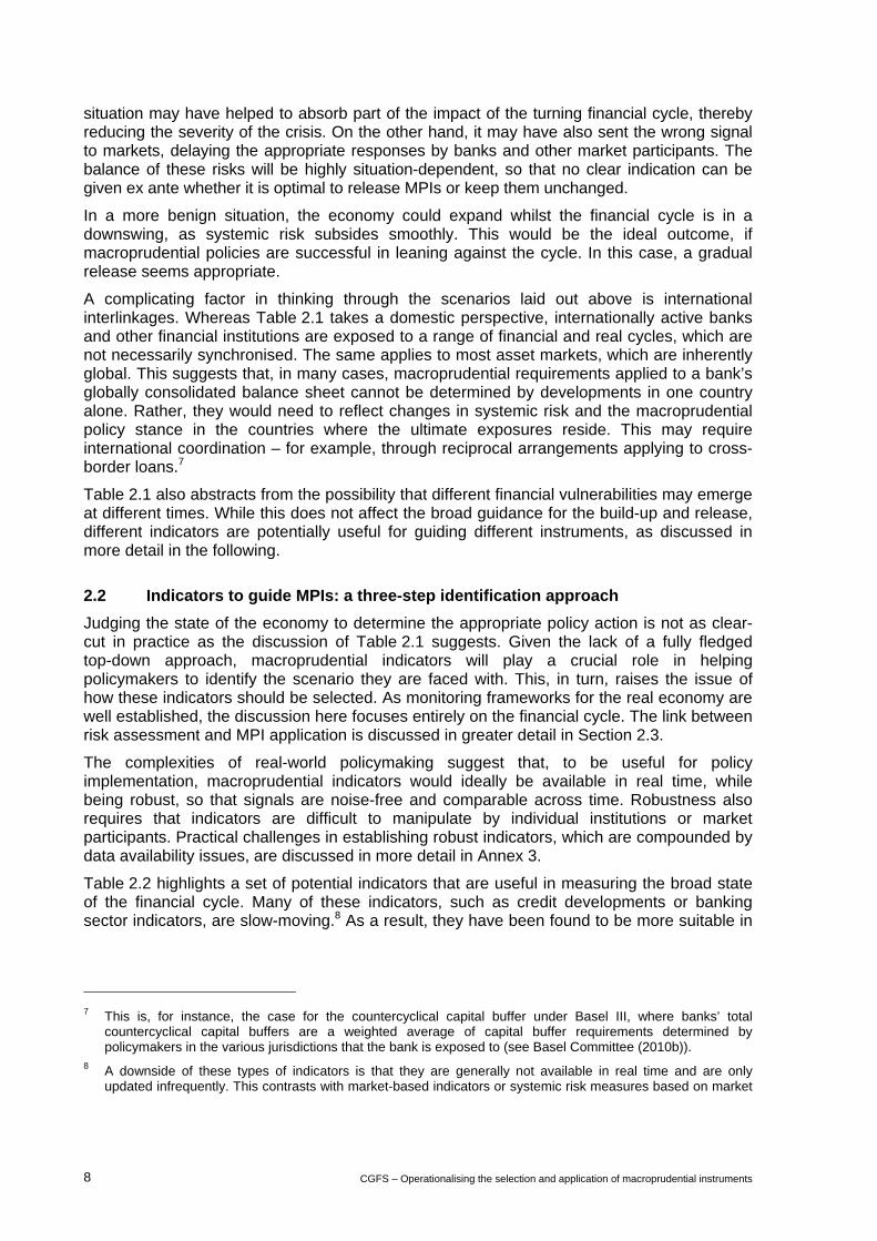
The next step in the selection of indicators is to break down cross-country evidence to the country-level. This step is illustrated below for the case of two candidate indicators: the credit-to-GDP gap and the price-to-rent gap. Both of these have been identified during the first stage of the analysis as providing useful signals in the build-up phase of the cycle. In addition, they are not highly correlated with each other. This suggests that their information could be considered complementary and should be combined using either judgment or statistical techniques (see Annex 3 for a description of how this could be done).

To highlight potential issues for country-level analysis, Graph 2.2 depicts the evolution of the two indicators around crisis periods for four countries (see Annex 3 for the remaining countries where both indicators were available). The vertical black lines denote financial crises and the vertical orange lines indicate other periods of interest, as discussed below. The red horizontal lines highlight the critical threshold, determined by statistical tests for the price-to-rent gap, while the green horizontal lines are the critical thresholds suggested under Basel III for the credit-to-GDP gap.

Graph 2.2

Price-to-rent and credit-to-GDP gaps for selected countries1


Price-rent gap2

Australia Switzerland Sweden United Kingdom

Credit-to-GDP gap3

Australia Switzerland Sweden United Kingdom

–40

–20

0

20

40

60

85 90 95 00 05 10–40

–20

0

20

40

60

85 90 95 00 05 10–40

–20

0

20

40

60

85 90 95 00 05 10–40

–20

0

20

40

60

85 90 95 00 05 10

–30

–20

–10

0

10

20

30

40

85 90 95 00 05 10–30

–20

–10

0

10

20

30

40

85 90 95 00 05 10–30

–20

–10

0

10

20

30

40

85 90 95 00 05 10–30

–20

–10

0

10

20

30

40

85 90 95 00 05 10

1 The black vertical lines indicate the beginning of systemic banking crises. The orange vertical lines indicate stress periods that did not result in crises. 2 The red horizontal line is the critical threshold (24 pps), determined by the statistical tests described inAnnex 3. 3 The credit-to-GDP gaps are based on bank credit to the private non-financial sector, using the same definitions as the countercyclical capital buffer guidance document (Basel Committee (2010b)). For Sweden, this includes lending from Swedish branches outside Sweden to non-resident entities. The green horizontal lines are critical thresholds as determined by Basel Committee(2010b). At 2 pps, the guidance given by the credit-to-GDP gap would suggest that buffers should start to accumulate. At 10 pps, thegap would suggest that buffers should have reached their maximum.


Overall, the graph confirms that both indicators provide useful signals, as suggested above, albeit with different lead and lag structures around crises. Comparing statistical cross-country evidence with a country-specific perspective, several issues stand out.

First, the indicators under consideration are imperfect in that they issue wrong signals (ie they may signal a crisis without one materialising and vice versa, as highlighted by the orange lines in Graph 2.2). In Switzerland, for instance, one major bank required government support during the recent global crisis, but the indicators presented here correctly identified no domestic vulnerabilities. The reason for this dichotomy was losses stemming from oversees exposures, rather than domestic vulnerabilities, highlighting the importance of cross-border positions for macroprudential policy purposes (see Section 2.1).

Equally, the build-up of vulnerabilities as signalled by the indicators does not necessarily mean that crises will erupt. This was, for example, the case in Australia in the early 2000s, where imbalances decreased after Australian authorities implemented a series of measures targeting the exuberant residential property sector, which could be considered macroprudential.15 Rather than mechanically relying on specific indicators, though, the Australian authorities used a broad a range of information and supervisory judgment.

Second, structural features might render an indicator inappropriate as a reference point for MPIs in a particular country. One example is the price-to-rent gap in Sweden, which would have signalled vulnerabilities persistently since 1998. The housing market in Sweden is, however, characterised by a high degree of regulation, with rents in the public housing sector effectively capping those in the private sector. As a result, observed rents generally do not reflect the market value of the rented units, implying that the price-to-rent ratio cannot provide reliable information.

2.3 Linking systemic risk assessment and MPI selection

An overarching question that policymakers have to decide on is whether they want to link systemic risk assessments and MPI application in a rules-based or discretionary fashion. The principal trade-offs of both approaches are also discussed in detail in previous reports, such as CGFS (2010a).

Rules versus discretion

A rules-based application relies on indicators to provide correct signals for the build-up and release. Given the identification problems described above, this can raise serious calibration issues. In addition and depending on the policy implementation, the Lucas critique may also apply, ie the underlying dynamics may change once the policy is in place. However, a rules-based approach has the benefit of being very transparent, is easily communicated and may act as a commitment device to “take the punch bowl away once the party gets going”.

Alternatively, policymakers may want to act in a discretionary manner. In this case, policymakers would typically try to use as much information as possible and rely on judgment in drawing this information together. In this context, warning signals issued by indicators would tend to act as triggers for deeper analysis, which could involve the use of more formal methods, such as stress tests (see Box 2 in Section 3 below) or full-scale financial stability

15 In particular, APRA undertook a rigorous industry-wide stress test in 2003 designed around a scenario of a

severe housing bust. The results of this test spurred it to introduce a more risk-sensitive capital framework for high risk exposures to the household sector and significantly raise minimum regulatory capital requirements for the mortgage insurance sector as well as tighten other prudential standards.


models.16 Practical experience has also shown that qualitative information can play an important role. For example, the implementation of macroprudential measures for the real estate sector in India was guided by supervisory judgment based on a softer type of information such as evidence of lax underwriting standards, a few fraud cases, anecdotal evidence of inventory build-up and emerging signs of underpricing of risks due to spiralling real estate prices (Table 2.6 suggests some questions that could be useful starting points to elicit this type of soft information during the build-up phase).

Table 2.6

Potential questions to provide qualitative information about the build-up of vulnerabilities

Are there signs of speculative behaviour?

Are particular asset classes heavily advertised or discussed in the media?

Are banks taking large positions where profits continuously exceed measured risks?

Are there relatively new products with large market shares, and have they been increasing rapidly?

Are lending standards falling?

Are profit margins decreasing?

Is competition increasing from the shadow banking sector?

Addressing measurement uncertainty

Measurement uncertainty is another issue that policymakers have to take into account. In part, this uncertainty is inherent to problems of measuring systemic risk, as fragilities emerge infrequently and often in new and unexpected ways. However, uncertainties also arise from problems common to other policy areas, such as delays in data reporting or conflicting messages arising from different sources of information.

The uncertainty of risk assessments has to be set against the cost of mistiming the application of MPIs. While the assessment of this trade-off is situation-dependent, policymakers can use different strategies to cope with it.

If the uncertainty is very large, but there is a clear sense of an underlying vulnerability, they may want to implement MPIs which are not time-varying.17 Similarly, if policymakers are confident that vulnerabilities are building up in a particular sector, sectoral capital requirements could be the appropriate tool. However, such an assessment would also need to take into account that spillovers from a small sector often tend to have broader, system-wide effects.18 In cases where uncertainties around the source of exuberance and potential spillovers are too large, a system-wide countercyclical buffer may be more appropriate. Alternatively, when the reliability of underlying risk weights is in doubt, a risk insensitive

16 For a survey of financial stability models for policy purposes, see Bisias et al (2012). For a more detailed

discussion of the advantages of two-stage frameworks for systemic risk monitoring, see Eichner et al (2010) and Cecchetti et al (2010).

17 See Annex 2 as to why this could be an optimal response in theory. 18 For example, a detailed analysis of spillovers from the household sector to the broader economy is provided

by Sveriges Riksbank (2011).


instrument such as a leverage ratio may be a useful tool. Another strategy to manage uncertainty in risk assessments is based on gradualism, which Asian policymakers have tended to rely on in their application of macroprudential policies. That is, policymakers may adjust MPIs in small steps and sufficiently early, retaining the ability to observe the impact and change the setting, if necessary.

Taking account of instrument characteristics and the policy process

The appropriate timing for the application of MPIs also depends on inherent characteristics of the instruments and the policy process. For example, once the legal and operational infrastructure is in place, LTV and DTI caps can be implemented rather rapidly. On the other hand, banks may need possibly several months to adjust to higher capital or liquidity requirements without being forced into fire sales or deleveraging, unless these are applied just to the flow of new lending (see Annex 5 for a discussion). The policy process may also take some time, as for example data are reported with lags. In addition, in many cases the application of MPIs does not completely rest with one authority, but measures are often discussed and information is shared among a group of relevant agencies through inter-agency groups, which may prolong the process further. These considerations favour starting the process of adjusting MPIs early, and relying on instruments for which knowledge about any implementation lags already exists.

3. The transmission mechanism of MPIs

To select the appropriate MPIs, policymakers have to judge which instruments can effectively and efficiently address an identified vulnerability. This section studies the conceptual transmission mechanism for a range of MPIs to illustrate key aspects of how the efficiency and effectiveness of instruments could be judged in practice.

As a practical tool, “transmission maps” are proposed to draw attention to the main transmission channels through which MPIs can achieve the macroprudential objectives of increasing resilience and leaning against the credit cycle.19 Both objectives are highlighted, even though the latter (“leaning”) is the more ambitious one, which, if pursued, implies a careful approach until more practical experience has been gained with the impact of MPIs on the credit cycle (see CGFS (2010a) and Box 1).

Where possible, the analysis is supplemented with empirical evidence to provide some indications of the effectiveness and efficiency of different MPIs, as a full cost-benefit analysis of different tools is likely to be highly state-dependent in practice and fraught with uncertainties in the absence of a usable top-down approach. The main aim of the discussion is, therefore, to provide a clearer narrative on the transmission channels through which the tools can achieve the two macroprudential objectives.

The build-up and release phases are analysed separately, as the dynamics may differ, starting with the tightening phase of capital-based, liquidity-based and then asset-side tools. Subsequently, potential interactions between MPIs as well as with other policy areas are discussed.

19 The transmission maps are stylised representations of the transmission mechanism of MPIs, highlighting the

key channels through which MPIs can achieve both macroprudential objectives. As such, they abstract from potential second-round effects, like the feedback from the credit cycle to output, which in turn may impact on leverage, asset prices and risk-taking.


3.1 Tightening capital-based MPIs

This section focuses on the tightening phase of countercyclical capital buffers as envisaged by Basel III, sectoral capital requirements, as well as dynamic provisions. These three MPIs are referred to as capital-based MPIs in the report.20 In addition, Box 2 discusses capital stress tests, which can be used to assess potential capital shortfalls.

A generic transmission map for capital-based MPIs is shown in Graph 3.1 (upper panel), reflecting the broad similarity of the transmission channels of the three different types of capital-based instruments. However, some differences remain. While aggregate, system-wide buffers are calibrated to ensure that the banking system as a whole is properly capitalised from a macroprudential perspective, sectoral capital requirements concentrate on the relative price of – and risks stemming from – lending to a particular sector in the economy (Graph 3.1, lower panel).21 Provisions, in turn, work through the profit and loss accounts of banks and are conceptually based on an assessment of impairments rather than unexpected losses. They may thus alter management’s incentives more directly than capital requirements.22

20 Macroprudential leverage ratios may be an alternative capital-based MPI. Their main benefit – but also main

drawback – is that they are not risk sensitive but based on capital relative to total assets. 21 Sectoral capital requirements can be operationalised in a number of different ways, as discussed in Annex 5. 22 An additional consideration is that capital requirements are fully within the realm of banking supervision. In

contrast, provisions are chiefly influenced by accounting practices.

Box 2

Stress testing

Stress tests have been used as a method to assess the resilience of banks and the banking sector for a while. Since the global crisis, stress testing has gained in prominence and in some countries, such as the United States, it has even been partly enacted in legislation. While stress testing is primarily a supervisory instrument, macro stress tests have the potential to reveal the build-up of financial system risks that might not be visible from standard supervisory information. As such, they can provide quantitative guidance on how capital levels should be adjusted. In addition, they can serve as the basis for coordinated, macroprudential disclosures aimed at reducing market uncertainty about risks related to the specified stress scenarios.

The transmission mechanics of stress tests are shown in Graph B1. The exercise begins with a stressed scenario. This is fed through a set of equations that forecast income and losses to determine net profits, which in turn determine bank capital. In the case of a shortfall, the transmission mechanism of tighter requirements is in line with the general case (Graph 3.1, upper panel). In normal conditions, stress tests imply that banks will be sufficiently well capitalised to be resilient against a severe but plausible downturn. When additional systemic risks are building up in a buoyant economy – because, for example, underwriting standards weaken – stress tests can result in higher pro forma levels of capital, as higher loss rates are likely to be revealed in the stress scenario. Thus resilience increases. If banks also internalise the (higher pro forma capital) cost of laxer lending standards, this may also slow their deterioration, any associated excessive credit growth, and thereby the build-up of systemic risk.

Conceptually, stress tests can assess various sources of systemic risk. Asset prices – such as residential or commercial real estate prices – can increase rapidly in buoyant times and present a common source of downside risk. Stress test scenarios can also be designed to address specific sources of systemic risk. For example, if systemic risk is building up on account of prices increasing


Graph B.1

Transmission map of stress tests

Purple cells = possible bank reactions; blue cells = possible market reactions.

1 SEO: seasoned equity offer.

very rapidly for only one class of assets, such as residential real estate, the scenario can be tailored to this asset class, leading to higher pro forma capital ratios for loans to the targeted sector. Stress tests also have the potential to capture various channels of contagion, such as fire sales and liquidity dry-ups. However, modelling uncertainties remain large, requiring sound judgement during the application as well as for the interpretation of stress tests.

_____________________ Macro stress tests can also be an effective crisis management tool. In this case, the US and European experience suggests that this requires the existence of a credible mechanism for any necessary recapitalisations. The variables that would typically be included in this scenario are activity variables (such as real GDP growth and the unemployment rate), asset prices (such as equity prices and real estate prices) and interest rates (such as short- and long-term government bond rates, corporate bond rates and mortgage rates).


Graph 3.1

Transmission map of raising capital or provisioning requirements

Transmission map of raising sectoral capital requirements

Purple cells = possible bank reactions; blue cells = possible market reactions. 1 SEO: seasoned equity offer. 2 The impact of tighter capital requirements for sector X on credit conditions in other sectors isambiguous. One the one hand, the quantity of credit in other sectors could decrease, if banks fulfill sector specific capital requirements by increasing spreads or curtailing credit across the board. On the other hand, the quantity of credit in other sectors may increase aslending to other sectors becomes relatively more attractive in comparison to lending to sector X.


3.1.1 Transmission maps for capital-based MPIs

The transmission maps illustrate the key transmission channels through which tightening capital-based MPIs can impact on the resilience of the financial sector and the credit cycle. Expectations-based implications for bank behaviour and instrument leakages are also highlighted – effects that can impact on both objectives.

Impact on resilience. Raising capital or provisioning requirements enhances the resilience of the banking system in a direct fashion. The additional buffers mean that banks are able to weather losses of a greater magnitude before their solvency is called into question, thus reducing the likelihood of a costly disruption to the supply of credit and other financial intermediation services. In addition, resilience may also be increased indirectly via the impact on the credit cycle and by affecting expectations and, hence, market participants’ behaviours and banks’ risk management practices.

Impact on the credit cycle. Banks have four broad options to respond to a shortfall in capital or provisions: (i) increase lending spreads, (ii) decrease dividends and bonuses, (iii) issue new capital or (iv) reduce asset holdings.

The first three options may negatively affect credit demand, as lending spreads are likely to increase. Higher lending spreads are a common response to increased funding costs, as implied by both a reduction in dividends and the issuance of new equity. Lending spreads are likely to be increased disproportionately for new and repriceable loans, as interest rates on outstanding loans are often fixed in many countries.

The fourth option leads to a reduction in the supply of credit, as banks may respond to tighter MPI settings by rationing the overall quantity of credit. One possibility is to restrict the extension of new credit across the board. Another, more likely one, is to shift the composition of assets towards exposures that carry lower risk weights or lower provisioning requirements.

The impact on credit conditions of tightening sectoral capital requirements is broadly similar to that of the other two capital-based MPIs. However, there are differences. First, higher sectoral capital requirements increase the relative cost for banks of lending to the specified sector, providing sharper incentives to reduce activity there. Second, banks may find it hard to raise external equity to fund lending that has been singled out by the macroprudential authority as particularly risky, increasing the pressure on banks to build up capital through retained earnings or by reducing the supply of credit – most likely to the targeted sector.

Expectations-based effects. Expectations are central to banks’ capital planning, risk management and lending decisions as well as to those of other market participants. As in the case of the monetary policy transmission mechanism, expectations are therefore likely to be a key part of the transmission mechanism for MPIs.

One factor that is likely to influence the power of any expectations-based effect is the strength of the policy signal. As the activation of MPIs is costly in comparison with financial stability policies that predominantly rely on communication and moral suasion, credibility is enhanced. Such a signal should thus have broader effects on lending standards and risk management practices, which will in turn increase the resilience of the system.

Another factor determining the impact of MPI activation is whether market participants understand the policymaker’s reaction function and interpret it correctly. If policy is predictable in this way, banks may change their behaviour in anticipation of policy actions – for example, by reducing exposures to sectors showing signs of overheating. These expectational effects may become stronger once a history of macroprudential policymaking has been established. This suggests that it may be useful to employ a small set of


instruments rather than a larger range of little-known tools that are similar, yet different and may be infrequently used. In addition, this underscores the importance of appropriate communication strategies as highlighted by Principle 7 in Annex 1.23

Leakages and potential unintended consequences. The possibilities for leakages and arbitrage are an important aspect of the transmission mechanism of MPIs. Part of the tightening of a capital-based MPI may become ineffective, if banks, for example, reduce any voluntary buffers one-for-one. But this effect has natural limits, suggesting that a gradual implementation may be useful to take account of these effects.

Some of the reduction in bank credit will also be taken up by non-bank intermediaries or internationally active banks that are not subject to the MPI.24 Large borrowers in developed markets, for example, may be able to substitute bank credit with the issuance of bonds and similar instruments. Cross-border sources of finance, in turn, can be tapped quite easily by all borrowers, including households.

Another example is outright regulatory arbitrage, which in practice often becomes apparent only once the MPIs are applied and market reactions are being observed (see Box 3). Banks may also try to dampen the impact of policy changes by gaming internal models to generate lower risk-weighted assets. This may happen already in normal times, but tightening capital requirements may increase these incentives.25 Gaming risk weights may occur in particular in response to increasing sectoral capital requirements, as only one part of a bank’s book is affected. Macroprudential supervisors, therefore, need to track regulatory arbitrage activity on an ongoing basis, which requires regular surveillance of key market participants and the ability to identify subtle trends or abnormal patterns in financial data reported by banks.

A useful approach to prevent regulatory arbitrage is to design simple rules that help improve regulatory compliance. As such leverage ratios could be useful complements to other capital-based tools which build on internal models to calculate risk weights. In addition, reciprocal arrangements are beneficial to containing cross-border arbitrage.26

An inappropriate application of MPIs to deal with the risks at hand could impair the resilience of the system as a whole. For instance, if the source of exuberance is general (eg due to abundant liquidity and aggregate mispricing of risk), raising capital requirements for some specific sectors may simply shift exuberance to other sectors – a “waterbed effect”. The correct identification of the underlying vulnerabilities is therefore critical for the use of these instruments (see Section 2.3).

23 To the extent that systemic risk can arise from coordination failures among different actors in the financial

system, signals from policymakers could also help to coordinate behaviour on better outcomes. Policy signals and expectations of future policy actions could, for example, alleviate pressure on individual banks to keep up with the behaviour of peers that are regarded as bellwethers or industry leaders, making it easier for them to step away from business activities in exuberant sectors.

24 As regulatory arbitrage via the shadow banking sector is a general problem beyond macroprudential regulation, steps are undertaken to strengthen the oversight of this sector (see eg FSB (2011)).

25 There is on-going work by the Basel Committee to assess the consistency in the measurement of risk-weighted assets in the banking and trading book.

26 In this context, in order not to affect banks’ choices of branching versus subsidiarisation, branches of foreign banks should be treated the same as subsidiaries.


Box 3

Avoiding regulatory arbitrage in practice

Regulatory arbitrage is an important consideration when designing MPIs in practice. In some instances, though, the scope for regulatory arbitrage becomes apparent only once the MPI is in place. For example, Singapore implemented LTV caps on corporate borrowers to dampen demand from this sector. An additional consideration was to prevent individual buyers from circumventing existing LTV rules by forming companies to purchase residential property. To avoid arbitrage, Singapore’s authorities also tried to implement simple rules. For instance, Singapore’s LTV rule is applied to individuals with one or more housing loans outstanding at the time of application rather than to housing loans obtained for investment purposes. While the latter are self-declared and can thus be open to subjective interpretations, the former are identified on the basis of an objective criterion, which can be readily measured.

In contrast, regulatory arbitrage activity that seemed possible when designing the MPI may not actually occur. In Hong Kong SAR, for example, borrowers that cannot access domestic bank credit due to LTV rules could in theory seek cross-border or non-bank funding. So far, the Hong Kong Monetary Authority’s surveillance work – which includes regular and close dialogues with banks and the monitoring of banking statistics – suggests that no significant cross-border arbitrage has been taking place in response to the MPIs imposed in Hong Kong SAR.

3.1.2 Empirical evidence27

The transmission maps suggest that applying capital-based MPIs is likely to effectively impact on the resilience of the financial sector and the credit cycle. For efficiency assessments, potential costs have also to be taken into account. A sense of the empirical effects of tightening capital-based MPIs is provided by a range of studies:

Impact on resilience. While the impact of higher capital ratios and greater provisions on the resilience of individual banks is self-evident, the same applies from a system perspective. There is clear evidence that dynamic provisions increase the resilience of the financial system and several studies show that the same is true for higher levels of capital. For example, based on a range of models, the Long-term Economic Impact Assessment (LEI, Basel Committee (2010a)) estimates that a 1 percentage point rise in capital requirements leads to a 20–50% reduction in the likelihood of systemic crises. In absolute terms, however, marginal benefits of higher capital ratios decrease with higher initial capital levels.

Impact on the credit cycle. Empirical evidence also indicates that capital-based MPIs are effective in affecting (i) the price and (ii) the quantity of credit, even though the uncertainty about precise magnitudes is relatively large.

First, several studies suggest that lending spreads could increase between 2 and 20 basis points in response to a 1 percentage point increase in capital ratios, depending on whether funding costs change in response to greater equity cushions due to their effect on the likelihood of failure (ie depending on whether the Modigliani-Miller theorem is assumed to hold or not).

Second, tightening capital-based MPIs seems to decrease the volume of credit in the economy. There is evidence that, in the short run, banks seem to respond to an increase in target capital ratios by making about a half to three quarters of the required change through an increase in capital and the remainder through a reduction of risk-weighted asset (RWA),

27 References to the relevant literature can be found in Annex 4.1.


of which in turn only half is in the form of reduced lending. This would imply that a bank with an initial capital ratio of 8% would decrease its lending by 1.5 to 3% for a 1 percentage point increase in capital requirements.28 Based on the increase in lending spreads and banks’ reduction in credit, the Macroeconomic Assessment Group (MAG (2010)) estimates that the median impact of increasing capital ratios by 1 percentage point is a reduction in lending by 1–2 percentage points. The evidence of the effects of higher provisions on the credit cycle is more mixed. While research indicates that they have been effective in this regard in Spain, this does not seem to be the case in Chile and Colombia.

The overall effectiveness of capital-based MPIs in affecting the credit cycle is, however, likely to be reduced by two factors. First, around 30–50% of the reduction in bank credit has historically been offset by an increase in lending by unaffected banks and other credit providers. Second, during booms it is not uncommon for real credit to grow by 15–25%, suggesting that capital-based MPIs would need to be tightened quite significantly to bring credit growth down to more normal levels.

Impact on output. The MAG finds that, in the short to medium run, the median impact of a 1 percentage point increase in capital requirements decreases annual GDP growth by 0.04 percentage points. In the long run, the LEI estimates that such an increases lowers long-run output by 0.09%, when the positive impact on the reduction of the frequency and severity of banking crisis is not taken into account.29 However, other studies find no long-run costs at all.

3.2 Tightening liquidity-based tools

In contrast to the capital-based MPIs described above, there is little consensus on the appropriate liquidity-based MPI to be chosen. The main reason for this is that microprudential liquidity regulation is still evolving, limiting the amount of practical experience with the use of such instruments relative to capital-based tools. Nevertheless, a variety of liquidity-based MPIs have been suggested or implemented, including countercyclical variations in the Liquidity Coverage and Net Stable Funding Ratios to be introduced under Basel III, minimum haircuts on repos and securities lending transactions, countercyclical margin requirements,30 macroprudential reserve requirements,31 and levies on short-term wholesale debt.32

Rather than going into the detailed nuances of each of these alterative MPIs, the following section assesses the transmission mechanism of liquidity-based MPIs in a generic fashion, based on a tool that requires banks to term out their funding and increase liquid assets.

28 If a bank with a capital adequacy ratio of 8% were to only adjust RWAs in response to a 1 percentage point

increase in capital requirements, it would shrink its RWAs by around 12%. 29 The LEI estimates that net benefits are positive for a broad range of increases in minimum capital ratios

relative to Basel II. 30 See CGFS (2010b) for a more detailed discussion of margin and haircut requirements, including their

countercyclical application. 31 Reserve requirements have been employed as MPIs by several countries. These can be understood as a tax

that will have implications throughout the economy, with impacts depending on whether borrowers or depositors will have to pay it. Evidence suggests that changing reserve requirements can have temporary effects on the price and quantity of credit (see Annex 4.2).

32 Korea decided to introduce a macroprudential levy on non-deposit foreign currency liabilities held by domestic and foreign banks, as these types of deposits are important for the Korean economy but have been very volatile in the two last crises. See Shin (2010) for theoretical considerations about the benefits of this approach.


3.2.1 Transmission map for liquidity-based MPIs

Similar to capital-based MPIs, the transmission map (Graph 3.2) illustrates the key transmission channels through which tightening liquidity-based MPIs can impact on the resilience of the financial sector and the credit cycle. As before, expectations-based implications for bank behaviour and instrument leakages are also highlighted, as these channels can impact on both objectives.

Graph 3.2

Transmission map of raising liquidity requirements

Impact on resilience. Raising liquidity requirements enhances the resilience of the banking system through direct and indirect channels. Direct effects result from the ability of banks to weather periods of liquidity stress more easily – by giving them the opportunity to sell assets whose prices remain stable or by enabling them to be less reliant on more volatile short-term funding. In turn, this will limit contagion effects and negative repercussions for the real economy. Like capital-based MPIs, resilience is also increased indirectly, via the impact on the credit cycle or expectations, which, in turn, may lead to a tightening of banks’ risk management standards.

Impact on the credit cycle. Banks will tend to respond to a rise in generic liquidity requirements by adjusting the profile of their assets and liabilities, using one or more of the following broad options: (i) replace short-term with long-term funding; (ii) replace unsecured with secured funding; (iii) replace illiquid with liquid assets; (iv) shorten maturities of the loan book; and (v) decrease (illiquid) asset holdings that require stable funding.



Stable funding is increased by reducing short-term funding and replacing it with longer-term funding. Alternatively, banks can shift from unsecured to secured funding, thus increasing asset encumbrance. Both options will tend to increase funding costs (at least in the short run, when the benefits of greater resilience are not yet taken into account). Replacing illiquid with liquid assets or shortening the average maturity of the loan book, on the other hand, will reduce banks’ earnings. In all these cases, banks are likely to increase lending spreads rather than accept lower profits that would lead to lower dividend or bonus payouts.

The last option is to reduce holdings of asset classes that require stable funding. Together with higher lending spreads, this implies that the overall volume of credit in the economy is likely to fall, even though long-term and illiquid lending would tend to be most affected.

Expectations-based effects. The expectational effects of changes in macroprudential liquidity requirements are likely to be very similar to those for capital-based MPIs. However, given the potential for a more direct impact of liquidity-based MPIs on asset markets, communication strategies would need to be adapted to not only target banks but asset market participants more broadly.

Leakages and potential unintended consequences. Liquidity-based MPIs may not be effective if they are absorbed by a reduction of voluntary buffers or if they are circumvented by arbitrage. The broad mechanisms are likely to be similar to those observed for capital-based MPIs, as described above.

Liquidity-based MPIs may also interact particularly strongly with the transmission mechanism for monetary policy, and possibly in an unanticipated fashion given a lack of experience (see also Section 3.5.2). For one, these instruments affect the demand for central bank liquidity and, hence, the ability to steer monetary policy operational targets in line with the intended policy stance. Furthermore, they may impact on the yield curve, and effects are likely to depend strongly on market conditions, such as the supply of liquid assets across different maturity buckets.33

Finally, the tightening of liquidity-based MPIs may shift some of the liquidity risk into the non-financial sector. For example, borrowers may find it harder to match long-term investments with long-term funding. They may therefore rely on the use of shorter-term finance, increasing their liquidity risk, which in turn may negatively impact the resilience of the financial sector.


As already suggested by the above discussion, applying liquidity-based MPIs can effectively impact on both resilience and the credit cycle. For efficiency assessments, potential costs have also to be taken into account. The empirical evidence on the transmission channels and effects of liquidity-based MPIs is, however, scarce and inference has to be drawn mostly from studies looking at the potential effects of Basel III liquidity requirements or reserve requirements.

33 Liquidity-based MPIs can temporarily affect the yield curve along two dimensions. First, to the extent that

banks adjust the maturity profile of their liabilities, the demand for longer-term funding increases, while that for shorter-term funding will decrease. This will tend to steepen the yield curve. Similar effects would arise if banks reduce their holdings of illiquid assets, pushing up the return required by holders of such instruments. Second, tightening liquidity-based MPIs will raise the demand for highly liquid assets, such as government bonds, across the maturity spectrum. Thus the yield curve may shift downwards more generally.



Impact on resilience. As in the case of capital, the impact of higher liquidity buffers on the resilience of banks is self-evident, but there is also evidence that liquidity-based MPIs can effectively enhance system resilience. The LEI (Basel Committee (2010a)) estimates that the introduction of the NSFR decreases the likelihood of systemic crises by 10–20%. Furthermore, simulation-based studies show that a cyclical application of LCR requirements can mitigate negative feedback spirals and thus enhance the resilience of the system in stressed conditions.

Impact on the credit cycle. There is evidence that liquidity-based MPIs could be effective in curbing the credit cycle, yet the uncertainty is large, given the scarcity of information. Studies assessing the impact of Basel III, as envisaged in 2010, suggest that the introduction of the NSFR could trigger a 14–25 basis point increase in lending spreads. The introduction of the LCR, on the other hand, is estimated to increase spreads by about 15 basis points, while reducing lending volume by approximately 3 percentage points.

Studies assessing the impact of higher reserve requirements also find that lending spreads increase and lending shrinks. However, effects seem to be transitory. Evidence for Latin America suggests that increased reserve requirements impact negatively on the provision of credit. But effects seem to last mostly two and at best 10 months, suggesting that such a tool would need to be recalibrated continuously.

Impact on output. With respect to the potential efficiency of liquidity-based MPIs, cost estimates by the LEI suggest that meeting the NSFR reduces steady-state GDP levels by 0.08 percentage points, when the positive impact on the reduction of the frequency and severity of banking crises is not taken into account.35 The MAG, in turn, estimates that introducing the LCR decreases GDP by 0.8 percentage points, falling to 0.1 percentage points after 8 years.

3.3 Tightening asset-side MPIs

Asset-side MPIs generally restrict the quantity of credit by tightening borrowing constraints for certain groups of borrowers. In practice, these MPIs often apply to residential mortgages, and are discussed here as such. They can also apply to other asset classes such as commercial real estate, which has for example been the case in India.

A key example of asset-side MPIs is leverage limits applying to individual borrowers, such as LTV (loan-to-value), LTI (loan-to-income) or DTI (debt-to-income) caps, which have been extensively used both as micro- and macroprudential instruments. LTV caps set a quantitative limit to the amount of mortgage credit granted for a given value of the house. LTI and DTI caps impose constraints relative to the income of borrowers. A generic transmission map is shown in Graph 3.3.

3.3.1 Qualitative transmission map for asset-side MPIs

As for the previous tools, the transmission map (Graph 3.3) illustrates the key transmission channels through which tightening asset-side MPIs can affect the resilience of the financial sector and the credit cycle. Again, expectations-based implications for bank behaviour and instrument leakages are also highlighted, as these channels can affect both objectives.

Impact on resilience. Asset-side MPIs increase the resilience of the banking system directly through decreasing both the probability of default (PD) and loss-given-default (LGD) of loans. First, restrictions on LTV or DTI ratios reduce PDs, as borrowers have higher buffers to

35 The LEI estimates that the net benefit of introducing the NSFR is an increase in steady-state output by 0.68%.


withstand negative shocks. Second, by restricting the amount that can be borrowed against the given value of a property, limits on LTV ratios restrict leverage and, in doing so, decrease LGD. As for the other tools, resilience is also increased indirectly via the impact on the credit cycle or expectations, which in turn, may lead to a tightening of banks’ risk management standards.

Graph 3.3

Transmission map of tighter asset-side MPIs

Impact on the credit cycle. Tighter LTV and DTI ratio caps restrict the quantity of credit by limiting the funding available for certain borrowers, reducing housing demand and increasing savings. In principle, house prices will tend to ease, reducing households’ ability to obtain credit and withdraw equity more generally. The demand for credit is therefore likely to fall more broadly.

The strength of these transmission channels may be moderated by the fact that LTV or DTI caps do not directly affect the cost of borrowing – they simply restrict the ability of a specific group to borrow. While this may constrain some households, it is also possible that the demand from others with sufficient wealth might continue to drive house price growth.

The ultimate impact (including second-round effects) of any change in LTV ratio caps may be quite sensitive to its initial impact on house prices, in particular when house price growth is disconnected from fundamentals. If LTV cap tightening is followed by an initial house price decline, LTV ratios will increase, reducing the scope for equity withdrawals and GDP growth, which may trigger further declines in house prices. If, by contrast, house prices continue to rise after the LTV cap is tightened, aggregate demand may continue to be supported by



equity withdrawals as LTV ratios fall. Both amplification channels might be stronger when house price changes are due to speculative demand.

Expectations-based effects. Adjustments in asset-side MPIs, just as other MPIs, represent a costly signal by the macroprudential authority and, as such, can help alter market expectations and risk management practices, thereby increasing resilience. In contrast to other MPIs, however, there is a risk of expectations playing a destabilising role in the case of LTV and DTI/LTI ratio caps under some circumstances. If caps are expected to be tightened, households might respond by bringing forward borrowing. House price growth might then accelerate, at least temporarily. These effects can be avoided by implementing caps over a short period of time.

Leakages and potential unintended consequences. There are likely to be three distinct channels for leakages to occur. First, there may be leakages to the unregulated sector and foreign banks.36 Second, arbitrage through non-mortgage (unsecured) top-up loans is a possibility. Uncollateralised top-up loans (eg from real estate companies) could also facilitate home ownership if LTV ratio caps are overly restrictive when creditworthiness is assessed on a broader range of indicators.37 Third, if households are constrained by asset-side MPIs, the structure of the housing market could evolve in ways countering the intended effect (eg via the emergence of part-purchase, part-rent models of home ownership). In such a scenario, underlying demand for housing would remain unaffected and, hence, house prices would be unlikely to react to changes in asset-side MPIs. This suggests that the use of these MPIs would have to be accompanied by tight market surveillance (see Box 3).38

Another potential downside to asset-side MPIs is that they will tend to directly impede some viable borrowers’ access to home ownership. They may also have broader distributional effects, which could pose difficulties from a political economy perspective and may have to be managed via mitigating policy measures (such as mortgage insurance). In addition, changing asset-side MPIs may affect the number of housing transactions. While this may be beneficial when turnover is high and the market shows signs of overheating, the decline in the number of transactions may have unintended effects in the form of increased price volatility, given that price discovery in the housing market is generally poor to begin with.


As for the other MPIs, the transmission maps suggest that tighter asset-side instruments enhance resilience and affect the credit cycle. This is supported by the empirical literature.

Impact on resilience. There is evidence that asset-side MPIs increase the resilience of banks by increasing the resilience of borrowers. Specifically, several studies find that tighter LTV caps reduce the sensitivity of households to income and property price shocks.

Impact on the credit cycle. The impact on the credit cycle is less well documented, as relatively few countries have instituted LTV and DTI restrictions in a macroprudential fashion. The available evidence suggests that imposing LTV and DTI caps during booms slows down

36 Potential leakages to the foreign sector depend upon the mechanism through which LTV caps are deployed. If

applied through “conduct rules”, they are likely to apply to at least all branches of foreign banks, still leaving the potential for cross-border borrowing. These rules are likely to differ by jurisdiction.

37 For example, a household with a low LTI ratio that is able to make a 10% down payment may present a lower credit risk than a household with a high LTI ratio that is able to make a 15% down payment.

38 The FSB (2012) has issued a set of mortgage underwriting practices, which are helpful in mitigating the risk of gaming LTV or DTI ratio caps.



real credit growth and house price appreciation. One recent study finds, for instance, that tightening LTVs or DTIs tends to reduce real credit growth by 1–2 percentage points and real house price appreciation by 2–5 percentage points. The latter effect on property prices is, however, not as clear-cut in other studies.

Impact on output. An overall efficiency assessment is hampered by the fact that there is no empirical evidence on the costs of asset-side MPIs to the broader economy. In comparison with other MPIs, costs could be more limited, as these tools only affect a specific proportion of borrowers. In addition, costs to these borrowers may be mainly in non-monetary terms, as they may not be allowed to obtain the housing they desire.

3.4 Managing the release phase

The discussion in this section focuses on the release of capital- and liquidity-based MPIs because the economics of releasing macroprudential LTV and DTI limits are likely to be different. The release of LTVs and DTIs mainly affects credit demand and not credit supply as is the case with capital and liquidity requirements. As such, their release should not occur with the onset of the crisis, but rather in the recovery phase following the end of the imminent stress period.

3.4.1 Qualitative transmission of the release

As a general principle, capital and liquidity buffers should be relaxed in a downswing of the financial cycle to prevent prudential regulation from being procyclical. To see this, consider for example banks that suffer severe losses on their loan portfolio. To maintain fixed capital ratios in the face of these losses and procyclical measurement of risk (eg due to VaR-type models), banks may be forced to deleverage by fire-selling assets and contracting the supply of lending to the real economy. This, in turn, would probably lead to further credit losses on banks’ loan portfolios, which would heighten the incentives to deleverage even further. By removing the need for banks to deleverage for regulatory reasons, the release of countercyclical capital buffers may help to dampen this powerful contractionary process by allowing banks to weather losses while maintaining the flow of new lending.

The dynamics of the release may, however, differ in crisis and non-crisis periods, which are therefore analysed separately in the following, even though it may be hard to differentiate between the two in real time in the early phases of the downswing (see the scenarios discussed in Section 2.1).

Release without a crisis. If there is no crisis but a downturn in the financial cycle, losses are likely to increase, but not to such a level that solvency and liquidity are questioned for the system as a whole. In this case, it is unlikely that market constraints will be binding. However, given higher loss rates and procyclical measures of risk, banks may still be forced to deleverage excessively unless MPIs are released. The transmission mechanism of such an orderly release is likely to be similar to that in the build-up phase, only in reverse.

Release during a crisis. Crises often start with an initial shock, triggering the realisation that potentially large losses and liquidity demands are imminent. If macroprudential buffers are sufficiently large to absorb these effects, their release could ensure the smooth functioning of the banking system. This would be the ideal scenario.

During a severe crisis, though, losses and liquidity demands would tend to exceed the micro- and macroprudential buffers accumulated by many financial institutions.40 In such a situation,

40 For example, in the global financial crisis of 2007–09, and the European sovereign crisis that started in 2010,

microprudential buffers were not adequate, in addition to the lack of macroprudential buffers.


policy measures that boost the level of bank capital and liquidity in the system may be necessary to restore the banking sector to health. For instance, the US Supervisory Capital Assessment Program (SCAP) (see Board of Governors of the Federal Reserve System (2009)) in 2009 required several large banks to raise capital through either retained earnings, new external equity or, as a last resort, capital injections by the state. Ultimately, this was the turning point for the US banking system during the recent crisis.

Should macroprudential buffers be released in such a situation, despite the need of the system as a whole for more capital and liquidity? Not releasing buffers may enforce deleveraging pressures because of the so-called ratcheting-up effect: markets could simply consider the total (microprudential plus macroprudential) requirements as a jump-off point for additional market requirements.41 Beyond anecdotal evidence that some of these effects are present, it is, however, difficult to provide any empirical estimates of their strength. Yet, they may not play out in full. Breaches of MPI limits are likely to lead to weaker supervisory penalties than breaches of minimum standards. For example, Basel III only envisages restrictions on dividend and bonus payments for banks that do not satisfy the countercyclical capital buffer rather than more intensive management interventions that are associated with breaches of the minimum.

If ratcheting-up effects are not present, a release could do little for overall credit conditions, as the effective constraint on intermediaries’ actions could be the market-determined one. In this case, the macroprudential authority could in effect find itself “pushing on a string”. But even in this case, a release is likely to affect expectations, which in turn can alter credit conditions in the economy.

Expectations-based effects. Expectational effects may be especially important for the release phase because of the crucial role of trust and confidence in these situations. The signalling effect is, however, difficult to gauge ex ante. On the one hand, a release could amplify crisis dynamics, if market participants perceive it as confirmation of the severity of the situation. On the other hand, it could have a calming effect on markets by signalling that there will be lower pressure for asset fire sales and deleveraging.

The timing of the release is likely to be critical for the balance of these risks. During non-crisis downturns, an early release before the cycle has really turned may provide a “second wind”, increasing imbalances further rather than contributing to an orderly adjustment. After a crisis, on the other hand, MPIs may need to be released to avoid excessive deleveraging and asset fire sales. Establishing indicators to guide the right timing of the release is therefore important (see Section 2.2), yet it is likely that judgment will have to play a major role, as crisis dynamics tend to differ substantially.

To manage expectations, the release is likely to be more effective, the greater the credibility of the MPIs. On the one hand, this argument favours the build-up of large buffers during the upswing, even though building up large buffers is potentially costly. On the other hand, the credibility of MPIs hinges on the credibility of the macroprudential authority itself. In particular without an established track record, this highlights that policymakers need to (i) convincingly identify emerging or crystallising vulnerabilities already during the boom and (ii) clearly communicate the rationale for policy actions in both phases of the cycle (see Annex 1, Principle 7).

It may also be useful to coordinate a release with crisis management policies in stressed conditions. For example, markets and banks may be more willing to use built-up liquidity

41 A ratcheting-up effect assumes that market requirements are not based on an absolute, independent

assessment about the economic situation of banks, but are set relative to official requirements.


buffers if liquidity backstops are also implemented by the central bank at the same time.42 In addition, the release is likely to be more effective if the macroprudential authority is willing to credibly commit to keeping requirements low for a pre-specified period of time, or conditionally until the threat of a credit crunch has passed. In this case, markets would understand that banks have sufficient time to rebuild macroprudential buffers before requirements are raised again. This will avoid forcing banks to hold voluntary buffers in anticipation of new requirements.

Macroprudential authorities should also ensure that regulatory minima are credible even during crises, as market participants have to be confident that meeting them is sufficient to safeguard the survival of banks once additional macroprudential buffers are released. One challenge in this context is that crisis dynamics can reveal flawed assumptions supporting the calculation of these requirements.43

3.4.2 Empirical evidence

The empirical evidence discussed in the previous sections also provides indications about the effects when MPIs can be released in an orderly fashion. As such, the release of MPIs should be effective in decreasing credit costs and increasing the quantity of credit. However, this assumes that the release phase is a mirror image of the build-up phase, which is unlikely to be the case as suggested by evidence for relaxing asset-side tools. So far, these potential asymmetries between the build-up and release phase have not been taken into account in most empirical assessments, limiting available evidence. As indicated by the positive effects of increased capital demands by SCAP in the United States in 2009, a potentially important asymmetry during crisis could be that higher capital levels may not reduce credit growth, as implied by the studies discussed in Section 3.1, but are beneficial, as they could be a prerequisite for restoring market confidence.

Given the short history of bank-based MPIs, evidence is particularly scarce for the release phase during crisis periods. The Spanish experience suggests that higher dynamic provisions can moderate the decline in credit that would eventuate when the economy weakens.44 However, in the Spanish case, the overall level of the provisioning turned out to be too small relative to the size of the housing market adjustment to have any significant effects.

3.5 Interactions

In the preceding sections, MPIs have been analysed in isolation, even though they will tend to interact with each other as well as with other policies (such as monetary, fiscal and regulatory policy) in practice. While a detailed analysis of these interactions is beyond the scope of this report, key aspects of such an assessment are highlighted in the following.

3.5.1 Interactions between different MPIs

The transmission maps presented above illustrate that all MPIs discussed in this report increase resilience, whilst also affecting the credit cycle. But rather than being substitutes,

42 See Turner (2012) on how such an “integrated policy response” between macroprudential authorities,

supervisors and central banks for releasing liquidity buffers could look. 43 For example, during the recent crisis, many of the Tier 1 capital instruments did not absorb losses as

anticipated. Equally, loss rates on structured products were enormously higher than assumed for capital purposes.

44 See Jiménez et al (2012).


individual MPIs will tend to be complements that can be used to address different aspects of systemic risk at the level of individual vulnerabilities. For example, both capital-based MPIs and asset-side tools limit the build-up of excessive leverage. Yet, the former target banks whereas the latter aim at the non-bank (typically, the household) sector.

In addition, recent theoretical research highlights potential interactions between macroprudential tools.45 For example, a change in capital-based MPIs may impact on house prices, which in turn affects the tightness of LTV policies. Equally, in response to tighter asset-side MPIs, banks may change their asset and liability holding, thus impacting on capital and liquidity requirements. The assessment of interactions is further complicated by the presence of a significant shadow banking sector. Tighter bank centred MPIs could for example lead to its expansion, which in turn could feedback into the overall liquidity conditions in the economy. Finally, some very simple interactions arise from the fact that higher capital ratios tend to reduce liquidity requirements and vice versa. This suggests that combinations of tools, rather than an individual MPI, should be considered when implementing macroprudential policies in practice.

This raises the question of how the optimal policy mix would be chosen in the absence of a fully fledged top-down approach (see Section 2). Any answer is likely to be highly country-specific, but one key factor is going to be the state of the cycle. During periods that are assessed as very exuberant, for example, it may be most prudent to not only constrain the build-up of leverage in the banking sector with capital-based tools, but also target borrowers more directly by, for instance, activating LTV or DTI caps. If excessive maturity transformation is also judged to be an issue, countercyclical liquidity requirements may be a possible complement, even though their efficacy remains uncertain.46 Such an approach could also guard against widespread regulatory arbitrage and waterbed effects that would otherwise drive exuberance into areas not directly targeted by an individual MPI. Gradualism, in turn, could help manage the uncertainties involved in implementation.

These considerations suggest that it would be useful for policymakers to have legal powers over a range of policy tools that can address the main sources of systemic risk in the time-series as well as the cross-sectional dimension. While the overall macroprudential toolbox needs to be comprehensive enough, a very broad toolbox also carries some risks. First, theoretical research suggests that uncoordinated application of several MPIs can be welfare-reducing, because tools can interact in unanticipated ways.47 Second, highly targeted MPIs should only be used with care, as otherwise their deployment may easily lead to attempts to micro-manage the economy, which failed in the 1970s. Third, communication challenges are amplified if policymakers rely on too many little-known tools that are similar, yet different, and may be infrequently used. Finally, overlapping tools targeting similar vulnerabilities, but having different reaches, can lead to unwelcome political economy dynamics, as there is likely to be pressure to apply the narrower tool, because it provokes less opposition and appears to be less costly. All these factors could reduce the effectiveness of MPIs and the public acceptability of using macroprudential tools more generally.

45 See De Nicolò et al (2012) and Goodhart et al (2012b). 46 The theoretical literature also advocates the use of countercyclical margin requirements to guard against the

build-up of systemic risks in the shadow banking sector (eg Goodhart et al (2012b)). However, implementing such a tool is highly challenging in practice, as there are for example serious risks of arbitrage.

47 See Goodhart et al (2012b).


3.5.2 Interactions between policy areas

The transmission maps presented in the previous sections suggest that the discussed MPIs influence the credit cycle and thereby also output and inflation. As such, these instruments are likely to affect the objectives of other forms of policy, such as monetary and fiscal policy (and in turn, these other policies could affect the objective of macroprudential policy). Annex 6 provides a conceptual discussion about possible interactions, while the discussion here focuses on practical considerations of assessing the scope of policy interlinkages and potential mechanisms for policy coordination.48

Assessing the scope for policy interlinkages

One aspect of the assessment of policy interlinkages is the degree to which the transmission channels for two policy areas are bound to overlap. For example, for monetary policy the balance sheet channel for firms may be impacted by asset-side tools, while the bank balance sheet channel potentially interacts with capital-based MPIs. Overlaps with the monetary policy transmission mechanism will tend to be particularly strong for liquidity-based tools (such as LCR-type buffers), which can affect the demand for central bank liquidity and, hence, the ability to steer monetary policy operational targets in line with the intended policy stance. The risk-taking channel more broadly is likely to be affected by all MPIs.

Another important consideration is to assess the conditions under which instrument settings for two respective policy areas may in fact conflict with, rather than complement, each other. This may be the case in scenarios where real and financial developments give rise to conflicting policy prescriptions (Scenarios 2 and 4 in Table 2.1). Frictions may also arise when the economy experiences “supply” shocks, such as periods of high productivity growth that put downward pressure on inflation but, at the same time, risk triggering irrational exuberance in financial markets. Equally, competition policies may work against financial stability enhancements. And the presumption of government support can represent a source of moral hazard and thus exacerbate risk-taking in buoyant times, which macroprudential policies aim to lean against. During a downswing, on the other hand, there may be tensions between macro- and microprudential objectives, as microprudential requirements may increase because of procyclical risk measures and higher loss rates. As discussed in Section 3.4.1, a release of MPIs may still be warranted, nonetheless.

An important practical question is also how often conflicts could materialise. From a historical perspective, financial crises tend to occur at a lower frequency than the business cycle. Consequently, most business cycles do not coincide with crises, which since the beginning of financial liberalisation have occurred on average about once every 20–25 years in any given country. This suggests that, most of the time, monetary and macroprudential policy decisions are likely to be adjusted at different rates, and conflicts are not necessarily frequent.49

In some cases, tensions between monetary and macroprudential policies can be eased if a longer time perspective is taken to evaluate monetary policy trade-offs. In a situation of low inflation and accumulating risks, for example, the apparent tension between a desire to cut interest rates to accommodate reduced inflationary pressures and to tighten macroprudential tools to contain a leveraged asset price boom might dissipate, once a longer-run perspective on price stability is taken.

48 Future work could provide more guidance for assessing the strength of interactions between MPIs and other

policy areas, as this is a relatively new research area. 49 Based on a theoretical model, Beau et al (2012) find, for instance, that conflicts between monetary and

macroprudential policies are rare.


While there are likely to be overlaps between the tools used by monetary and macroprudential policy, there are important differences too. Monetary policy relies on nominal instruments with short-term effects on real variables. It can address distortions in credit markets, but only indirectly. That said, it sets the universal price of leverage and thus touches all credit markets, not just those to which the macroprudential policy applies. This is an important consideration if in practice macroprudential policies can only affect regulated parts of the financial system and if there is significant leakage to unregulated sectors. In contrast, macroprudential policy tools can affect real variables in the long as well as the short run and address distortions in credit markets in a much more direct fashion. In addition, even to the extent that they have only a limited effect on excessive risk-taking or credit growth, MPIs increase resilience (see discussion above), which is not something monetary policy can provide.

Mechanisms for policy coordination

Given that policy interactions can affect instrument choice and application, even if such occasions may be relatively rare, central banks ought to monitor them closely. This would also suggest that, it could be useful, for example, to set MPIs and monetary policies in a cooperative fashion.50 At a minimum, appropriate mechanisms will have to be put in place to foster coordination. One aspect is policy mandates, which, however, come in various forms. If, on the one hand, a central bank’s mandate stipulates price stability as the main goal, financial stability considerations could be taken into account insofar as they affect the transmission mechanism of monetary policy. If, on the other hand, a central bank’s mandate is defined in broader terms, it may be desirable, for example, for monetary goals to cross-reference financial stability goals and vice versa. The monetary policy frameworks of the Bank of Canada and the Bank of Japan, for example, stipulate that long-term risks such as the effects of financial imbalances should be taken into account when aiming to achieve price stability. More recently, the UK government is proposing to provide the Financial Policy Committee with a secondary objective to support the economic policy of the government, subject to delivering a resilient financial system.

More generally and as highlighted by Principle 5 (Annex 1), the coordination problem indicates that central banks have to play a key role in macroprudential policymaking, either as leading agent or as part of an independent central agency, formal committee arrangement or similar institutional framework, appropriately reflecting national circumstances. In general, central banks are well placed to carry out macroprudential policy, due to their established analytical capacity for systemic risk analysis, expertise in market intelligence gathering from their market participation roles, and independence, which enables them to impose policy interventions that are unpopular in the short term. To underpin such a setup, the respective roles and independence arrangements for the two policy areas will need to be carefully and transparently specified.

4. Macroprudential policy in practice: questions and answers

This report seeks to provide practical guidance for the selection and application of macroprudential instruments based on three high-level criteria: (i) the ability to determine the appropriate timing for the activation or deactivation of the instrument; (ii) the effectiveness of the MPI in achieving the stated policy objective; and (iii) the efficiency of the instrument in

50 The optimality of cooperation between macroprudential and monetary policymakers is shown, for example, by

Adrian and Shin (2008), Angelini et al (2011) or Bailliu et al (2012).


terms of a cost-benefit assessment. In trying to operationalise these criteria, the report proposes a number of practical tools that can aid the assessment of individual MPIs.

Based on the analysis provided above, this final section breaks down these three high-level criteria into nine practical questions, which policymakers may want to consider when deciding on the selection and application of MPIs. While the relevant answers will depend in part on country-specific factors and are likely to require additional analysis, the analytical tools proposed in this report should help overcome at least some of the difficulties posed by operationalising macroprudential policies.

Determining the appropriate timing for the activation or deactivation of MPIs

1. To what extent are vulnerabilities building up or crystallising?

As highlighted in Section 2, the activation and deactivation of macroprudential instruments necessitate an assessment of financial vulnerabilities. To aid such an assessment, this report lays out broad scenarios in which MPI settings may be tightened or released. The identification of these states is facilitated by two alternative approaches that seek to link systemic risk analysis and MPI selection. Illustrative results are provided for a range of indicators to guide instrument use.

Exemplifying how to take account of cross-country evidence and country-specific factors, indicators that are helpful in identifying vulnerabilities in the household sector are assessed in more detail. The results could form part of the implementation of MPIs that target this specific vulnerability, such as maximum LTV settings, DTI caps or sectoral capital requirements related to household risk.

Depending on the preferences of the policymaker and the reliability of the chosen indicators, MPIs may be implemented in a rules-based fashion, where policy adjustments are guided by one or several indicators in a predetermined fashion. Alternatively, policymakers may want to act discretionarily using a broad range of information. In this case, practical experience has shown that qualitative information and supervisory judgment will be of great importance. Given the complexities of systemic risk assessments, fully rules-based implementation is likely to be limited to a small number of MPIs, even though rules-based signals can provide valuable input into discretionary decision-making processes for all instruments.

2. How (un)certain is the risk assessment?

Measuring vulnerabilities is always associated with uncertainty. This is partly inherent in problems of measuring systemic risk, as fragilities emerge infrequently and often in new and unexpected ways. Additional uncertainties arise from problems common to other policy areas, such as delays in data reporting or conflicting messages arising from different sources of information.

The uncertainty of risk assessments has to be set against the cost of mistiming the application of MPIs. These costs are generally asymmetric, as delayed action is generally more costly than a premature intervention. During the build-up phase, delayed activation may imply that MPIs are ineffective and a crisis materialises nonetheless. Implementing MPIs too early, in contrast, will tend to incur unnecessary regulatory costs and may weaken the impact, as market participants seek to develop avoidance and arbitrage strategies. During the release phase, on the other hand, easing MPIs prematurely may give markets the wrong signal, whilst releasing them too late may amplify procyclical effects, if, for example, banks have to deleverage more to satisfy additional macroprudential buffers.

In practice, policymakers can use different strategies to cope with this uncertainty. If uncertainty is large, but there is a clear sense of possible vulnerabilities emerging undetected, they may want to opt for MPIs that are not time-varying or measures that are risk insensitive such as leverage ratios. Similarly, if policymakers are confident that vulnerabilities


are building up in a particular sector, sectoral capital requirements could be the appropriate tool, whereas uncertainties over sectoral risk assessments and potential spillovers would argue in favour of a system-wide countercyclical buffer. Another strategy to manage uncertainty in risk assessments is based on gradualism, which has been heavily used in Asia. That is, policymakers may want to change MPIs in small steps and sufficiently early, retaining the ability to observe the impact and adjust the setting, if necessary. The same applies in situations where the transmission mechanism of the instrument is not entirely clear (see below) and when practical experience with a given instrument is limited.

Assessing the effectiveness of MPIs

3. Is there a robust link between changes in the instrument and the stated policy objective?

The transmission maps proposed in Section 3 can help policymakers assess the transmission mechanism for the instruments at their disposal, aid analyses of how changes in instrument settings will affect the ultimate policy objective, and highlight any interlinkages with other policy areas. Based on the illustrative examples provided, a robust link between adjustments in macroprudential instruments and the objective of enhanced resilience of the financial sector exists for a broad range of instruments. In contrast, in many cases this link remains more uncertain for the objective of leaning against the cycle.

A given instrument’s effect on system resilience depends on a variety of factors, which will have to be checked against the chosen objective. First, some MPIs may increase resilience more as they have a broader reach. For instance, countercyclical capital buffers build cushions against banks’ total credit exposures, whereas LTV ratio caps only affect new borrowers (and usually only those that are highly leveraged). This argues in favour of capital buffers if overall resilience is targeted, whereas LTV ratios would probably be chosen if concerns were focused on particular types of activities. Second, the degree of tightening is important, but the effects are not necessarily linear. For example, an additional percentage point of liquidity requirements will reduce the likelihood of default for highly liquid banks by less than for a bank that is closer to becoming illiquid. Third, in some states of the cycle, changing macroprudential requirements may be ineffective, as market constraints are binding. This will tend to be particularly important for the release phase.

The impact of MPIs on the credit cycle, in turn, is rather indirect and will tend to involve a variety of channels, which complicates any assessment of the effectiveness and efficiency of tools. The empirical evidence suggests that tightening MPIs increases lending spreads and decreases the quantity of credit. Yet, the uncertainties are large. For instance, liquidity-based instruments may have only temporary effects on credit conditions. Capital-based tools, on the other hand, may need to be tightened substantially to rein in a credit boom, in particular when taking account of possible leakages to unaffected credit providers. Uncertainties during the release are even larger, as there is little empirical evidence of such policy actions, in particular during crises.

4. How are expectations affected?

As is the case for the monetary policy transmission mechanism, expectations are likely to be a key part of the transmission mechanism for MPIs. If market participants understand policymakers’ reaction functions and interpret them correctly, they may change their behaviour in anticipation of future policy actions – for example, by reducing exposures to sectors showing signs of overheating. Expectations-based effects may be especially important for the release phase, because of the crucial role of trust and confidence during crisis periods. However, these effects are hard to gauge for MPIs that have a limited history or are only infrequently used.


To manage expectations, clear communication detailing the rationale for policy action is likely to be crucial (see also Annex 1, Principle 7). This also suggests that it may be useful to employ a small set of instruments rather than a large range of little-known tools that are similar, yet different and may be rarely used.

5. What is the scope for leakages and arbitrage?

In practice, there is always going to be scope for regulatory arbitrage and similar leakage effects, but some tools are more susceptible than others. For example, asset-side MPIs are less prone to international leakages because they tend to operate through conduct rules binding both domestic banks and foreign branches. Simple leverage ratios on the other hand are immune to arbitrage through changes in risk weights, which can be an issue for other capital-based MPIs.

International coordination is likely to be necessary to avoid cross-border arbitrage. Following the example of countercyclical capital buffers under Basel III, one possibility to enhance coordination is reciprocal arrangements, which could be institutionalised so that other macroprudential requirements – say, in the form of LTV caps or liquidity buffers – would also apply to cross-border exposures. Policymakers may also want to consider the harmonisation of the definition and design of macroprudential instruments. This may be particularly relevant for jurisdictions which are highly integrated (eg for currency unions).

The extent of leakages may become apparent only once the MPI is in place and evasive behaviours are being observed. Macroprudential policymakers, therefore, need to track regulatory arbitrage activity on an ongoing basis, which requires regular surveillance of key market participants and the ability to identify subtle trends or abnormal patterns in financial data reported by banks. A useful approach to prevent regulatory arbitrage is to design simple rules that help improve regulatory compliance and that are robust to “gaming” (see Box 3).

6. How quickly and easily can an instrument be implemented?

Timely execution has been one of the most important considerations when authorities decided to implement MPIs in the past, underscoring the importance of both legal frameworks and experience. To limit any implementation lags from the legal side, it would thus be useful for authorities to have legal powers over a set of policy tools that can be used to address the main sources of systemic risk in both the cross-sectional and time dimension. In addition, legal powers should also allow for flexible responses to contain possible new sources of systemic risk that are not tied to existing instruments.

Experience gained thus far, in turn, suggests that the time and ease of implementation also depend on the characteristics of the MPI, which may favour instruments that are already in use at the microprudential level and for which knowledge about any implementation lags already exists. For example, once the legal and operational infrastructure is in place, LTV and DTI caps can be implemented rather rapidly, given that many jurisdictions have ample experience with these tools at the practical level.

Assessing the efficiency of MPIs

7. What are the costs of applying a macroprudential instrument?

Implementing macroprudential policy instruments may entail short-term costs, in particular in terms of output losses. Overall, the broader the reach of the macroprudential tool and the tighter its setting, the more costly its application is likely to be, favouring narrower and more targeted interventions. However, various studies suggest that the costs of certain system-wide tools, such as higher capital requirements, may not be substantial in comparison with their likely benefits, implying that there is scope for these or similar tools to be calibrated with macroprudential objectives in mind.


The costs of adjusting MPIs are also partly determined by any administrative burden and costs in supervising the implementation. Again, this will tend to favour tools that build on existing microprudential frameworks, specifically when implemented with administrative considerations in mind. In addition, once a particular instrument has been chosen, MPI design and calibration can be based on the same considerations (see for example Annex 5, which outlines different possibilities for implementing sectoral capital requirements that differ substantially in the reporting burden for banks).

8. How uncertain are the effects of the policy instrument?

Uncertainties about the transmission channels may not only create difficulties in assessing the effectiveness of a particular MPI, they also create the potential for unintended consequences. Again, the use of transmission maps (see Section 3 for details) can help assess these effects, specifically for instruments that have already been used in practice and those building on established microprudential tools. Within this class of MPIs, in turn, policymakers will probably prefer those tools for which uncertainties within the microprudential (or other policy) framework itself are limited. Compared to other MPIs, this may argue against the use of countercyclical liquidity requirements, for which experience – at least at this time and at the cross-country level – is more limited. Yet, given the multifaceted nature of systemic risk, it is unlikely that policymakers can always adapt established tools to address specific sources of systemic risk.

As in the case of dealing with uncertainties in the appropriate timing, a practical option to manage uncertainties pertaining to instrument impact is to adjust MPIs in small steps and sufficiently early (“gradualism”), so that policymakers have the chance to observe the impact and adjust the setting as necessary. In addition, more empirical research about the effectiveness and costs of MPIs will be helpful in reducing this uncertainty.

Assessing the optimal mix of MPIs

9. What is the optimal mix of tools to address a given vulnerability?

Given an assessment about the state of the financial cycle, assessments of the effectiveness and efficiency of a given MPI determine the costs and benefits of intervention and can thus, in principle, be used to guide instrument choice. In practice, however, the nature of the vulnerability targeted and remaining uncertainties over MPI transmission may make it optimal to employ not just one tool, but a set of tools.

This raises the question of how the optimal policy mix would be chosen. While any answer will be highly country- and situation-dependent, a key consideration concerns the state of the cycle. During periods that are assessed as very exuberant, for example, it may be most prudent not only to constrain the build-up of leverage in the private sector – by for instance activating LTV or DTI caps – but also to target banks more directly with higher countercyclical capital requirements. If excessive maturity transformation is also judged to be an issue, countercyclical liquidity requirements may be a possible complement, even though transmission remains somewhat uncertain. Gradualism, in turn, could help manage the uncertainties involved in implementation, including the risk of regulatory arbitrage.


Annex 1: Broad principles for the design and operation of macroprudential policy

Principle 1: Systemic risk diagnosis should integrate supervisory information, market intelligence and aggregate indicator data.

Effective diagnosis is critical for macroprudential policy. It is needed to inform the assessment of emerging risks, the nature and extent of systemic fragility, the choice of instruments, the timing of intervention, and communication aimed at building public support for policy action. Without a sound evidence base, it will be much more difficult to calibrate fixed instruments, to design robust automatic or rule-based approaches, and to overcome the political hurdles to taking discretionary action.

Supervisory, market intelligence and aggregate information sources together provide a broad and complementary view over the financial system. Aggregate indicators help summarise system-wide developments, while detailed supervisory information and market intelligence, including insights from central banks’ operations in markets, enable judgment about the products and behaviours that are contributing most to systemic risk. Such a view is needed to detect the systemic risks and contagion-promoting features of financial behaviour that more fragmented supervision would miss. It is also needed to build the evidence base to support macroprudential, as opposed to microprudential, interventions.

The symptoms of growing systemic risk are likely to be many and various. At the same time, the information content of indicators may vary significantly across economies, depending on such factors as the level of development of the financial system and the strength of trends in the use of various types of credit. Authorities therefore need effective ways to identify relevant co-movements and common factors, to reduce the complexity of the assessment problem.

Principle 2: Interlinkages between financial institutions and markets, including cross-border exposures and associated hedging markets, must be monitored and understood.

Interlinkages between institutions and markets, both domestically and cross-border, can rapidly spread and massively amplify financial disruptions.

The ability for economically equivalent financial activity to move across sectors necessitates sharing of information across national supervisors. Especially to identify developments on, and migration of activity to, the fringe of the regulated sector, macroprudential supervision should be prepared to be intrusive. Developing systematic, timely and accurate data on these fringes is a priority.

Principle 3: Macroprudential authorities should at the outset develop instruments and policy for the financial infrastructure that fit the particular risks or imbalances diagnosed. Instruments could be based on fixed or variable capital and liquidity requirements, which are familiar from traditional microprudential policy, but also be restrictions on particular types of risk-seeking, or new tools.

A fairly comprehensive set of instruments is already available from the capital and liquidity requirements and restraints on particular types of risk-seeking familiar from microprudential policy. Policy settings can be either fixed or variable, and it is likely that both types will be needed. Tighter fixed requirements probably lessen the need for large adjustments of variable instruments, but are unlikely to eliminate the need entirely.


Such measures can be used flexibly to suit specific risk factors and their sources as they arise. Sector-specific measures might work better if banks are generally well capitalised, but the risk of sectorally or institutionally focused measures causing regulatory arbitrage needs to be recognised.

Building on familiar instruments when macroprudential policy frameworks are relatively new facilitates public understanding of macroprudential policy operation. A clearly identified set of instruments also helps create an onus on the authorities to use them, counteracting to some degree the lobbying pressures against intervention. Having said that, macroprudential authorities need to be alert to the risk consequences of financial innovation and to be ready to adapt instruments in response. With understanding of systemic risk dynamics still growing rapidly, macroprudential authorities should also be open to novel tools and measures to deal with a complex and evolving problem.

Principle 4: Intensive international information-sharing is likely to be needed.

Understanding risks and dependencies associated with the cross-border activities of internationally active banks requires arrangements among national authorities to share information, insights and financial stability assessments intensively. Such arrangements may need to include granular (firm-level) information on direct and indirect exposures and interlinkages among large players, across relevant financial markets.

The ease of avoidance of national measures in internationally integrated financial markets, and level playing field concerns, mean that the cross-border impacts of interventions taken by national authorities need to be understood and communicated.

Principle 5: Macroprudential policy should be the responsibility of an independent central agency, formal committee arrangement or similar institutional framework. It should be conducted either as part of the central bank or involving the central bank in a key role, appropriately reflecting national circumstances.

A centralised agency or arrangement facilitates the integration and rapid processing of supervisory and aggregate information from diverse sources, the coordination of measures imposed across broad classes of financial intermediaries if several regulatory agencies are involved in execution, the distinction of macroprudential from microprudential interventions, and the clarity and force of internal and external communications.

Central banks are well placed to carry out macroprudential policy, due to their established analytical capacity for systemic risk analysis, expertise in market intelligence gathering from their market participation roles, and independence, which enables them to impose policy interventions that are unpopular in the short term. In carrying out their roles in macroprudential policymaking, they will need to pay attention to the interaction between monetary and macroprudential policies. The respective roles and independence arrangements for the two policy areas will need to be carefully and transparently specified.

Principle 6: Macroprudential authorities should be charged with a clear mandate and objectives and given adequate powers, matched with strong accountability.

An explicit mandate bolsters the moral authority of policymakers to take unpopular actions and provides incentives for unbiased risk assessments. The mandate and independence need to be complemented by willingness on the part of the authorities to carry out policies that will be vigorously resisted during the benign part of the business cycle.


A good mandate should set relevant objectives. The objectives should be expressed precisely enough to be meaningful, but not so precisely that the development and flexibility of the regime to respond to evolving financial behaviour and to improving analytical foundations are constrained.

As part of countercyclical policy, leaning against the cycle to promote system resilience, as an explicit objective, can provide more scope to take pre-emptive actions. However, it could also raise expectations of what macroprudential policy should achieve, unless policymakers make clear that it is not an attempt to manage the credit cycle per se.

The powers of macroprudential authorities need to be adequate to cover the bulk of the financial system and to monitor the fringes of the regulated financial sector. Enforcement needs to be strong, especially when supervision of individual financial institutions is carried out by other agencies and as the regulatory intensity on the core financial system increases. Governance arrangements should allow for evolution of the regime over time.

Accountability measures are needed to balance broad powers and establish legitimacy. They can help frame an overall communications strategy for macroprudential policy.

Principle 7: Macroprudential policy communications strategies need to convey financial stability assessments clearly, link them logically to policy decisions, and manage public expectations about what can be achieved with macroprudential policy.

Clear financial stability assessments linked to policy decisions can help to create stabilising expectations. Communication can provide some of the benefits of quantitative rules if it can create a similarly transparent presumption of policy action clearly linked to systemic risk indicators and assessments.

To meet their mandates, macroprudential authorities will need to intervene at least occasionally. Given the diagnostic difficulties and uncertainty about the impact of macroprudential policy in practice, the expectations for macroprudential policymakers should not be initially too high. The durability of the regime requires that authorities build public support, including tolerance of mistaken interventions or non-interventions.

Such regime-building communication will face tough challenges. Among other things, policymakers will need to persuade the public that the obvious upfront costs of intervening now and then are outweighed by the less tangible benefits of keeping the risk of crises to a minimum.


Annex 2: Instrument and signal threshold selection: a conceptual framework51

This annex analyses instrument selection from a conceptual perspective. It highlights that macroprudential instrument selection and application are determined by:

the ability to determine the correct timing for applying an instrument;

the effectiveness of the macroprudential tool in achieving the objective; and

the efficiency of the tool, ie the cost of regulation relative to the benefits of intervention.

The annex looks at a highly stylised setting with two possible states of the world: (i) there are currently no vulnerabilities building up, or (ii) there are vulnerabilities, which will inevitably lead to a crisis in the next period. Policymakers can either impose MPIs or not.

Table A.2.1 summarizes the costs for policymakers depending on the state of the world and their actions. Starting with the world in which there is no crisis in the next period: if policymakers do not impose MPIs, welfare losses are zero, if they are activated, the economy faces the costs of regulation. However, if there is a crisis and no MPIs are imposed, the economy has to bear the full cost of a crisis. Finally, if a crisis materializes and MPIs are imposed, the economy has to bear the cost of regulation, but the cost of crisis is reduced by a factor α, capturing the effectiveness of the instrument.

Table A.2.1

Benefits and costs of using MPIs

No crisis next period Crisis next period

No MPIs 0 Cost of crisis

Impose MPIs Cost of regulation (1- α )Cost of crisis + cost of regulation

α is between zero and one and summarizes the effectiveness of the macroprudential tool

Given the costs and benefits of interventions, policymakers can decide to constantly impose a macroprudential tool, for example by raising minimum requirements. In this case, they do not have to measure systemic risk, and it may be an optimal response if measurement uncertainty is too large. As discussed in Section 2, the underlying vulnerabilities driving systemic risk can be measured to some extend in practice. However, there will always be instances where systemic risk will build up without being detected (a type 1 error (T1)) or measures will indicate systemic risk without it being present (a type 2 error (T2)).

The expected welfare costs can therefore be written as: E(Cost)= p(crisis) *(1-T1) * ((1– α)Cost of crisis + Cost of regulation) + p(crisis) *T1* Cost of crisis + (1–p(crisis)) * T2* Cost of regulation

51 This annex is based on Drehmann (2012).


Unsurprisingly, the expected welfare costs decrease with the effectiveness of the MPI (ie with higher α), with its efficiency (ie with lower costs of regulation) and with a more precise signal issuing fewer type 1 and type 2 errors.

This framework can help operationalising macroprudential policies in several dimensions, even though it does not take account of general equilibrium effects and potential interactions.

First, for given costs and benefits of a particular MPI, the framework helps to identify the optimal thresholds for a particular indicator variable, such as the ones discussed in Section 2.2.1 for instance. In this stylised framework, the optimal threshold is the solution to a welfare cost minimisation problem, assuming that policymakers mechanistically impose a MPI if the indicator variable breaches the threshold.

Alternatively, as costs and benefits of MPI use are hardly known, simulations can be run taking account of a broad range values for these parameters. An example of this kind of simulation is conducted by Drehmann (2012).52 Its main insights are quite intuitive.

The simulation shows that it is generally optimal for the policymaker to condition macroprudential tools on signals rather than considering only tools which are either permanently on or permanently off. This is not surprising. Even if a signal is not very informative, welfare is improved by, for example, switching buffers off in the few situations where policymakers are certain that they are not required as this saves regulatory costs.

The simulation can also provide some rough estimates of how often macroprudential tools could be implemented. Looking at countercyclical capital buffers and taking the credit-to-GDP gap as a an indicator that would be used mechanistically, the simulations indicate that it would be optimal to have the buffer switched on 3–40% of the time, depending on assumptions on the costs and benefits of intervention. The bulk of the simulations suggest quite frequent interventions, so that buffers would be on between 1 and 2½ years every 10 years.53

Lastly, the simulation framework can also be used to assess the optimal choice between instruments which differ in terms of costs and effectiveness. This is not an interesting question for two instruments where one is more effective and less costly than the other, as policymakers will always choose the first instrument. Yet, when there is a trade-off, the simulations show that it is optimal for policymakers most of the time to choose the instrument which is more effective, even when it is more costly.

52 The simulation in Drehmann (2012) uses three different parameters for the cost of crisis: 19%, 63% and 158%

relative to annual GDP. These costs are directly taken from the LEI (Basel Committee (2010a)). The annual probability of crisis ranges from 1 to 5%. The costs of regulation in the simulation broadly follow the results in the MAG and LEI: buffers lower annual GDP by 0.1%, 0.25%, 0.5%, 0.75% and 1%. As there is no real guidance on how effective macroprudential instruments are, the simulation simply assumes that the benefits of intervention (α) range from 5 to 75%. Finally, the simulation uses the credit-to-GDP gap as an indicator variable in line with the Basel III approach.

53 This is in line with the countercyclical capital buffer proposal in Basel III (Basel Committee (2010b)). This suggests that the credit-to-GDP gap should breach 10 percentage points to signal that buffers should be at their maximum. This happens around 15% of the time within the sample.


Annex 3: Indicators supporting the application of MPIs

This annex discusses methodological challenges in establishing robust indicators. It then performs a statistical assessment for indicators that are helpful in identifying vulnerabilities in the household sector on an individual basis and as combinations.

A.3.1 Methodological challenges in establishing robust indicators

There are several methodological challenges in establishing robust indicators in practice: identifying stress periods, pooling of countries and trending data.

Identifying stress periods. Much of the applied research aiming to identify indicator variables which can support countercyclical tools has largely assumed that policymakers desire reliable signals of future financial crises, as these events are closely linked with the objective of macroprudential policymakers. However, there is always a degree of judgment associated with when crises actually materialised. For instance, did the recent global financial crisis start in August 2007, when the money markets first froze? Or did it start with the Lehman failure? Or somewhere in between, when Northern Rock and Bear Stearns failed? Given that there are relatively few crises on which to calibrate, determining the timing of the crises can have a meaningful impact on indicator performance.

An alternative to using financial crisis dates is to use indications of financial stress such as those derived from a financial stress index (FSI). This more mechanical approach could allow for the identification of a predetermined threshold of an FSI that could be characterised as a stress period. This approach would provide some flexibility by allowing for signals to be calibrated using not only crisis dates but also periods of elevated financial stress (which could have potentially developed into a crisis). Given that it cannot necessarily be known when periods of stress will evolve into a full-blown crisis and the high economic cost of failing to identify a crisis in advance, the use of an FSI may be prudent.

However, an important drawback of such an approach is that there is no unique FSI. And those FSIs that have been constructed rely on financial market data, which are not always available in all countries, particularly in emerging markets. Furthermore, the threshold that delineates stress periods can change over time. Finally, while stress periods include all crisis dates, they will also include periods of stress that did not result in a significant impact on the real economy. For example, should indicator variables be partially conditioned on dotcom bubble crash, an event that, with the benefit of hindsight, suggests that it is unlikely that policymakers would have wanted to enlist the use of macroprudential tools?

Pooling of countries. Independently of whether crises or financial stress periods are used, periods of financial stress are rare. To use these scarce data efficiently, the academic approach has been to pool data and crisis dates across countries. While this is a reasonable strategy given the shortcomings of the data, practitioners should be aware that setting “global” thresholds ignores potentially important structural differences across countries. In fact, before employing global thresholds, it will be important for jurisdictions to determine appropriate country groupings with which to pool their data. Results suggest that altering the composition of countries within a pool can have a material impact on the threshold level and indicator performance.

Trending data. Many potential indicators shown in Tables 2.2 and 2.3 have trends. For instance, because of financial deepening, the credit-to-GDP ratio has an upward trend for most countries. Equally, property prices have trended upwards as the result of land scarcity and increased urbanisation. Therefore, in order to extract a signal of an imbalance, researchers have to decide how to detrend, keeping in mind that the detrending method has to be applicable in real time. A simple solution is to use growth rates. Researchers have also


used rolling averages, time trends or statistical filters. In these cases, the question remains as to how much historical data should be taken into account to construct the trend series. On the one hand, financial cycles tend to be quite prolonged, ranging from 10 to 20 years.54 On the other, financial innovation may change key characteristics of an indicator, which would indicate a shorter horizon. Empirically, many researchers have erred on the side of using historical information to construct a longer time trend to pick up on the robust empirical regularities before crisis build-up.

A.3.2 Indicators for the household sector

Following the signal extraction methodology proposed by Kaminsky and Reinhart (1999), Table A.3.1 provides a statistical examination of the performance of various indicators associated with the household sector, using a three-year flexible forecast horizon. The underlying idea is simple: a particular indicator will give a signal if it breaches a predefined threshold. A signal is considered correct if a crisis occurs at any point within the following three years. Otherwise, it is a false warning. The noise-to-signal ratio is the fraction of false warnings relative to the fraction of correct signals. The lower this ratio, the better the signalling quality of the indicator. As the costs of false warnings are much lower than those of failing to predict a crisis, a full grid search over potential thresholds was undertaken for each indicator to select the one that keeps the noise-to-signal ratio to a minimum while predicting at least two thirds of the crises.55 The statistical examination is best viewed as a description of which indicators would, with hindsight, have performed best in the set of countries examined. The credit-to-GDP gap, the

Table A.3.1

The statistical performance of different indicators1

Threshold

Fraction of false

positives

Fraction of crises

predicted

Noise-to-signal ratio

Credit-to-GDP gap 11 8 67 12

Household credit-to-GDP gap 3 22 75 29

Annual growth rate of real household credit – 15-year rolling average 3 21 75 28

Aggregate debt service ratio – 15-year rolling average 5 5 67 8

Annual growth rate of real residential property prices – 15-year rolling average 13 12 75 16

Residential property price-to-rent gap 24 9 63 14

1 Thresholds for indicators are chosen based on minimising the noise-to-signal ratio, conditional on capturing at least two thirds of the crises over a cumulative three-year horizon. A signal is issued if the indicator breaches the shown threshold. A signal is correct if a crisis occurs in the next three years; otherwise it is a false warning. The noise-to-signal ratio is the fraction of false warnings relative to the fraction of correct signals.

54 See eg Aikman et al (2010) or Drehmann et al (2012). 55 See Borio and Drehmann (2009) for a more detailed discussion of this issue.


debt service ratio, the growth of residential property prices and their gap are useful indicators for signalling crises. The worst performers are the variables involving household credit. In comparison to other indicator variables assessed in the literature, though, all these indicators demonstrate fairly good signalling qualities (see eg Drehmann et al (2011)).

A cross-country assessment of indicator performance around crisis periods provides useful guidance for identifying indicators for both the build-up and release phase. However, as discussed in Section 2.2 structural differences may imply that indicators which perform well on the whole may not be as effective for each country. As such, a deeper assessment at the individual country level is necessary when operationalising the use of indicators for specific MPIs.

A.3.3 Multiple indicator approach

In practice, macroprudential policymakers do not make decisions using a signal from one indicator but rather assess a broad range of indicators in order to form a judgment about the appropriate macroprudential policy actions. The combined information that arises from investigating the joint behaviour of the indicators generally provides a better signal than relying on a single indicator. For example, if price-based measures, leverage-based measures and credit growth-based measures all signal the build-up of imbalances, the macroprudential supervisor should have more confidence in triggering the appropriate tool. In contrast, if housing credit growth is high, but housing prices do not exhibit above-trend growth, a policymaker might draw a different conclusion.

Policymakers generally use judgment in aggregating indicators of imbalances to form a view of systemic risk. However, the literature has also suggested statistical approaches (eg Borio and Lowe (2002) and Borio and Drehmann (2009)).

Examining the correlation among various indicators allows an assessment of whether something can be gained from combining multiple indicators. One would expect more gains to be attainable through a combination of variables that perform well individually but are not highly correlated.

There are various approaches to tackling multiple dimension signalling. Two examples are weighted signalling and multidimensional grid search.

A.3.3.1 Weighted signalling

Weighted signalling constitutes the creation of a new variable by taking a linear combination of the original indicators and applying the standard signal extraction approach that is used in the one-dimensional case. One noteworthy application of this would be to incorporate the signal reliability of different indicators into a single variable by weighing those variables by their noise-to-signal ratio and using those weights as coefficients in the calculation of the new linear combination. It is, however, not clear, whether indicators should be combined in an additive fashion, or whether there are more complex interactions, which may be better captured with a non-parametric approach, such as a multidimensional grid search.

A.3.3.2 Multidimensional grid search

The multidimensional grid search approach is an extension of the one-dimensional case to multiple dimensions. Rather than optimising one threshold for one variable, n thresholds are simultaneously optimised for n variables. When all n variables breach their respective thresholds, a signal is sent. Alternatively, one could require only a certain number (m<n) of breaches to trigger a signal. Since these thresholds are determined simultaneously, rather than individually, the threshold for any one indicator could diverge in this context relative to its value on a standalone basis (and they will tend to be lower).

To give a more concrete sense of how this would work, the two-dimensional case using the credit-to-GDP gap and a measure of the price-to-rent gap is examined in Graph A.3.1. The


credit-to-GDP gap and price-to-rent gap are chosen as both variables perform well on a standalone basis and are not highly correlated with each other.

In the graph, the horizontal line separates crisis signals (above) from non-crisis signals (below) associated with the credit-to-GDP gap. Equally, the vertical line separates crisis (right-hand side) from non-crisis (left-hand side) as indicated by the price-to-rent gap.

The graph highlights that combining the credit-to-GDP gap with the price-to-rent gap (ie by considering only crisis signals which are in the upper right-hand corner of the graph) eliminates many false warnings, whilst removing few cases, where crises would have been predicted by one of the two indicators on a standalone basis.

Graph A.3.1

Multidimensional signalling

A multidimensional crisis signal is issued if the credit-to-GDP gap is larger than 5.5 (horizontal line) and at the same time the price-to-rent gap is larger than 6 (vertical line). Red (blue) dots indicate data points that are associated with a crisis (no crisis) in the following two years.

Sources: Bank of Canada calculations; national data.

–40

–20

0

20

40

60

–80 –60 –40 –20 0 20 40 60

Cre

dit-

to-G

DP

gap

Price-to-rent gap

No crisisCrisis


A.3.4 Additional country graphs

Graph A.3.2

Price-to-rent and credit-to-GDP gaps1


Price-to-rent gap2

Canada Germany Spain France

Credit-to-GDP gap3

Canada Germany Spain France

1 The black vertical lines indicate the beginning of systemic banking crises. The orange vertical lines indicate stress periods that did not result in crises. 2 The red horizontal line is the critical threshold (24 pps), determined by the statistical tests in Annex 3. 3 The credit-to-GDP gaps are based on credit to the private non-financial sector, using the same definitions as the countercyclical capital buffer guidance document (Basel Committee (2010b)). The green horizontal lines are critical thresholds as determined by Basel Committee (2010b). At 2 pps, the guidance provided by the credit-to-GDP gap would suggest that buffers should start to accumulate. At 10 pps, the gap would suggest that buffers should have reached their maximum.

–40

–20

0

20

40

60

85 90 95 00 05 10–40

–20

0

20

40

60

85 90 95 00 05 10–40

–20

0

20

40

60

85 90 95 00 05 10–40

–20

0

20

40

60

85 90 95 00 05 10

–30

–20

–10

0

10

20

30

40

85 90 95 00 05 10–30

–20

–10

0

10

20

30

40

85 90 95 00 05 10–45

–30

–15

0

15

30

45

60

85 90 95 00 05 10–30

–20

–10

0

10

20

30

40

85 90 95 00 05 10


Graph A.3.2 (cont)

Price-to-rent and credit-to-GDP gaps1


Price-to-rent gap2

Japan Korea Netherlands United States

Credit-to-GDP gap3

Japan Korea Netherlands United States

–40

–20

0

20

40

60

85 90 95 00 05 10–40

–20

0

20

40

60

85 90 95 00 05 10–75

–50

–25

0

25

50

85 90 95 00 05 10–40

–20

0

20

40

60

85 90 95 00 05 10

–30

–20

–10

0

10

20

30

40

85 90 95 00 05 10–30

–20

–10

0

10

20

30

40

85 90 95 00 05 10–30

–20

–10

0

10

20

30

40

85 90 95 00 05 10–30

–20

–10

0

10

20

30

40

85 90 95 00 05 10

1 The black vertical lines indicate the beginning of systemic banking crises. The orange vertical lines indicate stress periods that did not result in crises. 2 The red horizontal line is the critical threshold (24 pps) determined by the statistical tests in Annex 3. 3 The credit-to-GDP gaps are based on credit to the private non-financial sector, using the same definitions as the countercyclical capitalbuffer guidance document (Basel Committee (2010b)). The green horizontal lines are critical thresholds as determined by BaselCommittee (2010b). At 2 pps, the guidance provided by the credit-to-GDP gap would suggest that buffers should start to accumulate. At 10 pps, the gap would suggest that buffers should have reached their maximum.


Annex 4: The empirical strength of transmission channels

This annex provides a survey of the empirical literature to shed light on the strength of various transmission channels highlighted in the transmission maps shown in Section 3.

A.4.1 Capital-based tools

The evidence is divided into three categories: the impact on resilience, the impact on the credit cycle and the impact on output.

A.4.1.1 Impact on resilience

Empirically and theoretically, higher capital ratios and greater provisions increase the resilience of individual banks – this can, for example, be easily seen in Merton-type models. It is therefore not surprising that system resilience also increases with tighter capital- based tools. Looking at the experience of Spain, Colombia and Peru, Fernández de Lis and García-Herrero (2010) conclude that dynamic provisions help to increase the resilience of the banking system, which is confirmed by Chan-Lau (2012).

Based on a range of models, the Long-term Economic Impact Assessment (LEI, Basel Committee (2010a)) estimates that a 1 percentage point rise in capital requirements leads to a 20–50% reduction in the likelihood of systemic crises. In absolute terms, however, the marginal benefits of higher capital ratios decrease with higher initial capital levels. For instance, raising capital ratios from 6% to 7% decreases the annual probability of crises from 7.2% to 4.6%. Increasing capital ratios from 10% to 11%, on the other hand, decreases the annual probability of crises from 1.4% to 1.0%. Similar effects are found by Miles et al (2011), who show that increasing capital ratios from 5% to 10% reduces the probability of crisis from 7.0% to 2.5%.

A.4.1.2 Impact on the credit cycle

The discussion here is split into the impact of higher capital or provisioning requirements on (i) the cost of funding for banks, (ii) bank lending spreads and (iii) the quantity of credit.

Impact on banks’ funding costs

In theory (and without tax distortions), raising capital requirements should not lead to an increase in lending spreads, because the cost of equity funding for a bank would decrease as it becomes less risky (ie the Modigliani-Miller (1958) theorem would hold). There is clear empirical evidence that, in practice, issuing equity is costly from a private cost perspective. (see eg Asquith and Mullins (1986) or Gao and Ritter (2010)). These results, however, may primarily reflect a “signalling channel”: firms are likely to issue equity when their equity is overvalued, so that a seasoned equity offering may therefore signal such overpricing to the market (see eg Baker and Wurgler (2002)). One way of controlling for this effect is to study involuntary equity issuances – for instance, when the regulator demands that a bank raise additional equity. The evidence here is more mixed. Keeley (1989) examines capital issues by banks during the period 1975–86 and finds that involuntary stock issues produce a significantly more negative return than voluntary issues, suggesting that regulation-induced increases in capital could result in larger negative announcement effects. On the other hand, Cornett and Tehranian (1994) and Cornett et al (1998) find post-issue stock returns following an involuntary issuance to be broadly in line with benchmarks. Elyasiani et al (2011) compare Troubled Asset Relief Program (TARP) capital injections with seasoned equity offerings (SEOs) and find that investors reacted negatively to SEOs but positively to TARP.


In a similar vein, a robust finding of the large empirical finance literature on dividends and the market value of firm stocks is that the market reacts positively (negatively) to announcements of dividend increases (decreases). However, these studies focus on voluntary changes to dividends, which are likely to give rise to a similar “signalling channel” to that outlined above.

Overall, it is therefore unclear how applicable these results are for understanding the transmission mechanism of capital-based macroprudential policies, where capital is being increased at the behest of the macroprudential authority based on an assessment of building systemic risks (which depend on economy-wide conditions rather than firm-specific circumstance) rather than representing a decision by firms based on their financial position.

Impact on bank lending spreads

The Macroeconomic Assessment Group (MAG (2010)) used two approaches to quantify the impact on lending spreads of higher capital requirements. One approach posited an error correction model, in which the change in lending spreads was regressed on capital requirements, the prevailing level of lending spreads and a set of control variables. The other calculated the change in lending spreads required to keep the return on equity constant under the assumed capital ratio, given current quantities of loans and liquid assets, rates of returns on those assets, and current debt and equity funding costs. The median increase in lending spreads across both approaches in response to a 1 percentage point increase in the target capital ratio was roughly 15 basis points after 18 quarters and 16 basis points at the end of the simulation.56 Of the 14 models that estimated lending spread effects, 11 concluded that the end-period rise in spreads for this scenario would be between 5 and 23 basis points.

The LEI found similar results: a 1 percentage point increase in the capital ratio leads to a 15 basis point rise in lending spreads over the long term. These results are also consistent with those in Elliott (2009), who, using an accounting-based approach, concludes that each percentage point increase in the target capital ratio leads to a 19 basis point increase in lending rates, if other variables remained unchanged. Similar results are found for Latin American countries (Terrier et al (2011)). The only outliers seem to be Brazil and Chile, where the impact of a 1 percentage point increase in capital ratios is estimated to increase lending spreads by 5–6 percentage points.

All of the above results are based on the assumption that debt costs remain unchanged given higher capital ratios (ie the Modigliani-Miller theorem is violated completely). This is contentious. Hanson et al (2011) argue that, as leverage falls, the risk of debt also declines and this offsets the cost of having to finance the bank with a greater share of equity. Indeed, at the extreme (where the Modigliani-Miller theorem holds given no taxation), the reduction in the risk and cost of equity would exactly offset the effect of the increased weight on more expensive equity in the capital structure. The empirical literature on how SEOs affect corporate bond spreads is, however, quite minimal. Elliott et al (2009) is one paper that looks at this – albeit for non-financial companies only – and finds that SEOs do reduce bond rates, although this is only for the most risky types of debt.

Taking account of the effects of the Modigliani-Miller theorem, the literature finds much smaller effects, roughly of the order of a sixth to a third of the size of those reported above. Meisenzahl (2011) finds no significant effect of funding costs or capital ratios on business loan interest rates in small business loan data: specifically, for banks with more than $50 billion in assets in the 2003 Survey of Small Business Finances survey sample, he finds that a 1 percentage point increase in the capital ratio raises the business loan interest rate only 2.3 basis points (and this increase is insignificant). Likewise, Hanson et al (2010) report

56 Results are reported for a four year implementation period, but are very similar if this is shorted to two years.


a modest loan interest rate increase of at most 3.5 basis points for a 1 percentage point increase in the capital ratio. Similar effects are found by Miles et al (2011). They estimate bank lending spreads to increase by 4.5 basis points, whereas firms’ overall borrowing cost rise by less than 1.5 basis points, as bank lending represents only around one third of firms’ total financing.

Impact on the quantity of credit

The MAG also looked at the question of how higher capital might reduce RWAs, albeit in the context of permanently higher capital ratios. Using a variety of different modelling approaches, this study found a median estimated decline in lending volumes in response to a 1 percentage point increase in the target capital ratio of roughly 1.4% after 18 quarters relative to the baseline scenario, and 1.9% by the end of the simulation. 57 Of the nine models that included estimated lending volume effects, seven predicted a decline in volumes by the end of the simulation of between 0.7 and 2.1%.

The UK FSA found that UK banks would respond to an increase in their target capital ratio by making about half of the required change through a reduction in risk-weighted assets and the other half through an increase in capital. About half of the reduction in RWAs in turn is in the form of a reduction in lending. Berrospide et al (2010) found that large US banks would respond by making about one quarter to one third of the required change through a reduction in risk-weighted assets.

Another notable study in this literature is that of Aiyar et al (2012). They run bank-level loan regressions examining how supervisory firm-specific changes in bank capital requirements (that resulted from a special feature of UK bank regulation) altered lending growth. The effects they find are considerably larger than were found by the MAG study. Specifically, depending on the approach taken to control for loan demand effects, they find that a 1 percentage point increase in supervisory capital ratios implies a 6–9% reduction in loan growth.

Drehmann and Gambacorta (2011) undertake a simulation to analyse how the countercyclical capital buffer might have affected bank lending in Spain in the run-up to and during the crisis. They find limited effects in the upswing: under the counterfactual, annual credit growth would have remained well above 10% from 2000 onwards, peaking at around 23% in 2006. However, simulated bank lending would have been 2% higher in 2008 and 2009 had the buffer been released in the last quarter of 2007.

There is also evidence that the negative real sector implications of higher capital ratios need not be material. In a cointegration analysis for Germany, Buch and Prieto (2012) find no negative impact of bank capital on loans to private non-banks (business loans) in the long run.

Surveying the available evidence, Terrier et al (2011) conclude that the effects of dynamic provisions on the credit cycle are ambiguous. In the case of Latin America, dynamic provisions seem to have no impact on the credit cycle (Fernández de Lis and García-Herrero (2010), Chan-Lau (2012)). Jiménez et al (2011), on the other hand, find that they helped to mitigate procyclicality in Spain.

There is also an expanding dynamic stochastic general equilibrium (DSGE) literature on financial frictions, regulatory policy and their effect on bank lending, which could in principle also address the question of how higher capital might affect RWAs. Examples of these models are Christensen et al (2011), Angeloni and Faia (2012), Gertler and Karadi (2011),

57 Results are reported for a four year implementation period, but are very similar if this is shorted to two years.


Gertler et al (2011) and Kiley and Sim (2011). While this literature is making strides, there are a number of aspects of these models that call for a cautious approach to their use in trying to gauge the separate and combined effects of the various transmission channels. Each model takes a very stylised view of the role of banks that revolves around one or more market failures, and the choice of which market failure is considered in the model has a significant influence on the results that obtain regarding the effects of capital regulation. In this vein, it is also worth highlighting that, with the exception of Angeloni and Faia (2009), bank fragility does not feature in these models, so there is no real motivation for regulators to strengthen bank resilience. Rather, the sole motivation for regulators in most of these models is to moderate swings in the credit cycle. Moreover, only a few papers allow for multiple sources of bank financing, and no papers allow for any bank choice of assets apart from bank loans. Likewise, bank credit is typically the only source of funding available to non-financial agents.

These features of existing DSGE models mean that, in terms of the transmission maps, the “Options to address capital shortfalls” box in these models would contain only a very small number of alternatives. In addition, in these models the transmission channel between RWAs and credit would be direct and without any scope for leakages. Similarly, there would be no scope for credit to leak outside the banking sector. Also, the “impact on resilience” goal of policy is less relevant in this setup.

Of course, none of the above-described concerns rules out the possibility of using any DSGE model to undertake macroprudential policy analysis. Rather, the concerns suggest that, at the current juncture, DSGE models are too parsimonious to be able to give predictions about the quantitative strength of various channels.

A.4.1.3 Impact on output

Empirical assessments show that the output costs of higher capital requirements are rather modest.

Taking the median across different simulations, the MAG concludes that a 1 percentage point increase in the target ratio of tangible common equity (TCE) to risk-weighted assets would lead to a maximum decline in the level of GDP of about 0.19% from the baseline path, which would occur four and a half years after the start of implementation (and equivalent to a reduction in the annual growth rate of 0.04 percentage points over this period), followed by a gradual recovery of growth towards the baseline. In the long run, the LEI estimates that such an increase decreases long-run output by 0.09%, with a range from 0.02 to 0.35%, when the positive impact on the reduction of the frequency and severity of banking crisis is not taken into account. Including also the benefits of higher capital regulation, the LEI estimates that net benefits are likely to be positive for a broad range of increases in minimum capital ratios relative to Basel II.

These studies, however, assume that the Modigliani-Miller theorem is violated, so funding costs are permanently higher for higher capital ratios. If this is not the case, Miles et al (2011) find that a 1 percentage point increase in capital ratios reduces long-run GDP by less than 0.04%. The results of Buch and Prieto (2012) would suggest that there are no permanent effects on output in the long run at all, as they do not find any long-run effects of bank capital on loans to the business sector.

A.4.2 Liquidity-based tools

Quantitative evidence on the strength of transmission channels for liquidity-based MPIs is hardly addressed in the literature, due to the fact that most of the tools are not yet implemented. However, some inference can be drawn from studies looking at the potential effects of Basel III liquidity requirements or reserve requirements. As for capital-based instruments, the evidence is split into (i) the impact on resilience, (ii) the impact on the credit cycle and (iii) the impact on output.



The LEI estimates that the introduction of the NSFR decreases the likelihood of systemic crises by 10–20%, depending on the initial capital levels. Were the NSFR to equal 112%, the probability of crises would decrease by a further 40%.

Van den End and Kruidhof (2012) consider the systemic implications of a cyclical application of the LCR in a liquidity stress-testing model, which takes into account the impact of bank reactions and second-round feedback effects. They show for a hypothetical banking sector that a flexible approach of the LCR, in particular one which recognises less liquid assets in the buffer in times of stress, is a useful macroprudential instrument to mitigate its adverse side effects during times of stress. Lowering the minimum level of the LCR in times of stress delays the number of banks breaching the LCR requirement and thus the development of negative feedback spirals. Hence, a cyclical application of the LCR increases resilience.


The LEI estimates that the introduction of the NSFR could lead to a 25 basis point increase in lending spreads (without adjusting RWAs), while the effect is dampened to 14 basis points when taking the synergies of liquidity and capital regulation into account. Looking at the effects of new liquidity regulation in New Zealand, Terrier et al (2011) show that the introduction of these rules increases lending rates by 10–20 basis points.

In contrast, the report by the MAG considers a 25% increase in the holdings of liquid assets relative to conventional loans as a proxy for the introduction of the LCR. While the median increase of lending spreads is about 15 basis points, the median contraction of lending volume is approximately 3.2%.

Drawing on the experience in Latin America, there is evidence that reserve requirements increase lending spreads. For instance, Gelos (2009) finds that increasing reserve requirements on demand deposits by 10 percentage points increases net interest margins by around 0.4 to 0.7 percentage points. For Brazil, there seems to be evidence that reserve requirements can affect bank interest rates on loans with little impact on loan default rates, while there also seem to be implications for banks’ and non-financial companies’ stock returns (Carvalho and Azevedo (2008)). In another study on Brazil, Evandro and Takeda (2011) conclude that reserve requirements lead to a contraction in credit for households, especially from smaller banks.

Employing vector autoregression (VAR) techniques and using a sample of Latin American countries, Tovar et al (2012) find that increasing reserve requirements impacts negatively on the provision of credit, but only for one to two months and to a very limited extend. Looking more closely at Brazil, Glocker and Towbin (2012) find transitory effects lasting around 10 months.

A.4.2.3 Impact on output

As for higher capital requirements, the impact of higher liquidity requirements seems to have a modest impact on output. However, the evidence here is rather limited.

Focusing on the LCR, the MAG estimates that a 25% increase in the holding of liquid assets relative to total assets implemented over four years, combined with an extension of the maturity of banks’ wholesale liabilities, is associated with a median decline in GDP in the order of 0.08% relative to the baseline trend after 18 quarters.

According to the LEI, introducing the NSFR leads to a median fall in output of 0.18 percentage points. However, if synergies between higher capital and liquidity requirements are taken into account, the estimated median impact amounts to an additional 0.08 percentage point fall in output. But this turns into a gain of 0.68% when taking a reduction in the frequency and severity of banking crises into account and assuming a


moderate permanent effect of a crisis (with no permanent effect this decreases to 0.15%, and with large permanent effects increases to 1.83%).

A.4.3 Asset-side tools

There exists a large body of academic literature on the theory and evidence of LTV and LTI/DTI restrictions. However, there is no evidence on the potential costs of these policies.


There is evidence from Hong Kong that asset-side tools increase the resilience of the system. In Hong Kong, maximum LTV limits have been in place since 1991 and maximum DTI limits since 1997. LTV limits vary depending on the value of the property and whether it is to be owner-occupied. Craig and Hua (2011) and Wong et al (2011) find that tighter LTV policy reduces household leverage and the sensitivity of defaults to changes in property prices.

Indirect evidence from looking at micro data more directly supports this conclusion. Following the theoretical work of Stein (1995), a number of authors have looked for evidence of the amplification of shocks when households are more leveraged (as measure by LTV ratios). Lamont and Stein (1999) use city-level data in the United States and find that cities where a greater fraction of households have high LTV ratios are more sensitive to income shocks. Almeida et al (2006) perform a similar exercise, except that they consider a cross section of countries. They find that, in countries where households can obtain loans with higher LTV ratios, housing prices and new mortgage credit are more sensitive to income shocks. Wong et al (2011) also considered cross-country evidence and found that LTV policy reduces the sensitivity of defaults to changes in property prices.

Finally, some authors have considered the role of certain subsets of borrowers. Duca et al (2010) show that house price appreciation is sensitive to the LTVs of first-time buyers. First-time buyers are often cited as one of the groups of borrowers that would be most affected by LTV and DTI caps. Haughwout et al (2011) show that there was a large increase in the investor share of house purchases and subsequent delinquencies during the recent boom-bust cycle in the US housing market. Finally, Wong et al (2011) document the extensive use of mortgage insurance in Hong Kong, suggesting that LTV caps are binding on a number of (constrained) borrowers.


Relatively few countries have instituted LTV and DTI restrictions as MPIs. Consequently, the few papers that do investigate the effects of these policies concentrate on a particular set of countries. These empirical results should be taken as suggestive, as it is difficult to identify causal effects since these policies are activated during times of market exuberance and therefore changes are not exogenous. Moreover, they are often used in concert with other tools, including those related to the supply side of the housing market. Finally, there are often only short time series and the majority of the relevant variables are highly persistent.

Igan and Kang (2011) investigated the efficacy of Korea’s use of LTV and DTI caps. In Korea, maximum LTV limits have been in place since 2002 and maximum DTI limits since 2005. LTV limits vary depending on property value, region and type of loan. These authors find that tighter LTV/DTI policy tends to slow both transaction activity and property price appreciation, with the impact on activity being much stronger. In addition, using survey data, they find that expectations of price appreciation and speculative activity are suppressed by tighter policy. However, the authors find little evidence that relaxing LTV constraints has significant stimulative effects.

Hong Kong’s experience (Craig and Hua (2011) and Wong et al (2011)) suggests that there may be a limited impact of tighter LTV policy on property price appreciations.


Looking at more than 60 countries from 1980 onwards, Kuttner and Shim (2012) find that changing LTV and DTI limits are effective in limiting credit growth. Tightening these instruments tends to reduce real credit by 1–2%. They also show that these instruments have pronounced effects on price growth. They find that, in the short run, tightening LTV ratios reduced house price appreciation by 2%, whereas the effect in the long run could be up to 5%.

Comparing the effectiveness of LTVs and DTIs, Kuttner and Shim (2012) find that maximum LTV ratios and exposure limits are not as powerful as maximum DTI ratios. In their view, these effects stem from the fact that borrowers can borrow more given a fixed LTV ratio if house prices increase, which in turn tends to push up house prices further. However, the DTI ratio is anchored to income growth which is not easily amplified even during economic booms.

Indirect evidence on micro data also supports the fact that asset-side tools are effective in impacting on the credit cycle. In a series of papers, Mian and Sufi (2009, 2011) utilise variation in the cross section of US localities before and after the recession/financial crisis to study the role of leverage. They find that variation in household leverage, as measured by the DTI ratio, before the recession has strong predictive power for a number of economic variables after the recession. Mian and Sufi (2009) find strong evidence that credit supply and elasticity of housing supply exerted a key influence on the degree of leverage.


Annex 5: How to operationalise sectoral capital requirements?

Implementing macroprudential sectoral capital requirements raises a number of operational issues, even though the tool has been used by Australia, India and Switzerland among others. Additional sectoral capital requirements could in principle take a number of forms: raising the Pillar 1 sector risk weights directly through a multiplicative scalar; raising the floor under risk weights for certain exposures; or imposing capital buffer add-ons.

A.5.1 Changing sectoral risk weights

Sectoral risk weights can be changed in at least two ways: by applying a multiplicative scalar to microprudential risk weights, or by changing the sectoral risk weight floors.

A multiplier could be applied to banks’ microprudential risk weights on the sector in question. An advantage of this approach is that it is designed to work with the grain of current microprudential rules and keeps relative risk rankings constant within the sector. The multiplicative scalar is also a transparent and direct mechanism for increasing the capital requirements for the targeted sector.

An alternative way of operationalising sectoral capital requirements might be to introduce a lower bound for the risk weights on particular sectoral exposures. For example, the macroprudential authority could mandate that mortgage risk weights cannot be lower than X%. This approach would be similar to the Basel I floors currently in place. However, this approach is likely to change the relative risk weights within the banks’ portfolio and can potentially be distortionary. Furthermore, such floors are likely to be applied at the aggregate level, which may encourage banks to risk up within the sector in question.

A potential communication challenge associated with both approaches is that boosting risk weights will mechanically reduce banks’ reported capital ratios, and market participants may find it hard to disentangle what is driven by risk-taking behaviour by the bank and what is the result of the macroprudential tightening.

One way to get around this problem might be to have two different sets of reporting standards, with banks continuing to report the microprudential risk weights. This would allow the reported capital ratios to have the same interpretation as now, facilitating comparison over time and across institutions. However, having to keep track of two sets of capital ratios will add a layer of complexity to the process and would be costly for banks.

A.5.2 Sectoral capital buffers

Both the approaches outlined above envisage changing risk weights. In line with countercyclical capital buffers in Basel III, an alternative would be a capital add-on for each bank, depending on its exposure to the sector in question. This approach would leave the current RWA framework untouched and therefore not change the interpretation of banks’ capital ratios. In this regard, it would be simple from a communications perspective. However, this would be akin to a Pillar 2 treatment, which may raise some practical challenges.58

58 For example, in the United Kingdom the Pillar 2 add-ons are a part of the FSA’s Supervisory Review and

Evaluation Process (SREP), which is staggered over time for different banks, with a review period of


A.5.3 Stocks versus flow

Increased risk weights could be targeted at the flow of new lending or at the existing stock of lending. The choice of the tool here will depend partly on the objective: if the intention is to increase the resilience of the banking sector, it may be more appropriate to raise capital on the stock of loans; on the other hand, if the intention is to lean against exuberance in current lending, it may be better to target the flow. Applying a higher risk weight to the stock clearly covers both existing and new lending, and would be simpler to administer. Applying it to the flow might enable sharper targeting of the increase but would be administratively more complex both for firms and for the regulator, and could be more easily arbitraged.59

It might also inhibit refinancing and would require a very precise definition of what constitutes “new lending”.

A.5.4 Challenges once the tool is operationalised

Since the tool is designed to target exuberant sectors that are likely to be earning large returns for participants, and in light of the moral hazard issues associated with singling out particular sectors, decisions regarding this tool may become politicised.

There is also currently no reciprocity over this tool. So sectoral capital requirements would be subject to four sources of potential cross-border leakages: (i) lending via foreign branches; (ii) direct cross-border lending; (iii) lending from non-bank financial companies; and (iv) intragroup corporate lending. Finally, and as discussed in Section 3.1, regulatory arbitrage may undermine the effectiveness of this tool.

12–18 months depending on the bank’s importance. If this practice continued, this approach would lag actual books and be implemented across the banking system in a staggered way.

59 Conceptually, add-ons could also apply to a particular tranche of lending. Yet this would require the tranche to be forever separately identifiable, which is not practical unless loans were discrete, with a known start and end date. In addition, the system could be easily gamed by revolvers, extensions or credit commitments.


Annex 6: The interaction of macroprudential instruments with other policies

An important concern in the practical implementation of macroprudential policy tools is how these tools interact with other forms of economic policy, such as monetary policy, fiscal policy and structural policy (including microprudential policy). This annex explores these issues in greater detail.

A.6.1 The interaction of macroprudential policy and monetary policy

MPIs and monetary policy can impact on each other’s objectives through several channels. First, as is evident from the discussion of the transmission channels in Section 3, macroprudential policy tools can influence the price and quantity of credit in the economy, which in turn is likely to affect overall economic activity. But the latter is a key concern for all monetary authorities, independently of whether they have an inflation target or a dual mandate. Equally, real economic activity and the level of interest rates itself influence systemic risk – for example, via the risk-taking channel60 or the effect that economic growth has on variables such as financial institution leverage, asset prices and, more broadly, risk-taking. As a result, the monetary policy stance may affect macroprudential policies.

Second, MPIs may also interact with the monetary transmission mechanism.61 For example, suppose that monetary policy is loosened – due to conditions in the macroeconomy – at the same time as a capital-based macroprudential policy tool is deployed – due to the build-up of systemic risk. In this case, the deployment of a capital-based macroprudential tool will work – at least with regard to economic activity – against the bank balance sheet (or bank lending) channel. This is because the bank balance sheet channel relies on the resulting stronger economy generating an increase in bank capital via retained earnings that will in turn result in an expansion of credit. But if a capital-based macroprudential tool is being deployed, the increase in bank capital that results from monetary policy is likely to be directed towards satisfying higher capital requirements rather than boosting credit volumes.

Lastly, monetary and macroprudential policymakers will base their decisions in practice on similar data, pointing to potential interactions. For example, financial conditions such as valuation measures, lending conditions and credit aggregates are important information sources for monetary policy, and would of course constitute core inputs to macroprudential policymaking (eg see Section 3.2). On the other hand, the macroprudential policymaker would also take the state of the business cycle and the stance of monetary policy into account in setting macroprudential instruments.

The fact that macroprudential and monetary policy can impact on each other’s objectives raises two issues. First, which policy is better at achieving which objective? Second, do policies complement each other or do they conflict – and, if so, how often?

60 To date, the risk-taking channel has generally referred to low interest rates inducing increased risk-taking via

search for yield. The risk-taking implications of monetary policy actions are, however, broader. In general, the view is that lower interest rates or stronger growth induce greater risk-taking. As such, the risk-taking channel is one way in which monetary policy is transmitted to the real economy via financial institutions’ behaviour. That said, it is not infeasible that sluggish economic growth associated with weak financial institutions could induce gambling for resurrection and greater risk-taking.

61 See Beau et al (2012) for a detailed overview.


Following the research by Mundell (1960, 1962) and others in the context of fiscal versus monetary policy, the literature emphasises that policy tools should be assigned to the policy objectives where they can exert the most direct effect. There is broad consensus that monetary policy is better able to influence economic activity while MPIs are better suited to affecting the build-up of systemic risks. In addition, only MPIs can increase the resilience of the financial sector. Yet, as the previous discussion has made clear, each of the policies should take the stance of the other one into account when decisions are being taken.

The second question is whether macroprudential policy and monetary policy complement each other or conflict. Scenarios discussed in Table 2.1 indicate that MPIs and monetary policy often complement each other rather than conflict. For example, macroprudential policymakers would want to use MPIs and monetary policy would want to tighten at around the same time if systemic risk is building up when the economy is operating at above full employment. Theoretical research by Angelini et al (2011) indicates that, in such situations, employing MPIs in addition to monetary policy can enhance welfare considerably, in particular if both instruments are set in a cooperative fashion. Moreover, if each policy were to take account of the other policy’s action, each might be able to benefit from the other’s effect on its objective, thus allowing smaller adjustment in both policy levers.

Yet there can also be conflicts – for example, when real and financial developments give rise to conflicting policy prescriptions. Frictions may also arise when the economy experiences “supply” shocks, such as periods of high productivity growth that put downward pressure on inflation but, at the same time, risk triggering irrational exuberance in financial markets. Based on a DSGE model, Angelini et al (2011) find that, in these cases, macroprudential policy generates only modest benefits for macroeconomic stability over a “monetary policy only” world. A lack of cooperation between both sets of policymakers may even result in conflicting policies, leading to suboptimal outcomes.

As there is a potential for conflicts, the question arises as to how often this could be the case. Beau et al (2012) find, for instance, that conflicts are rare. Based on a DSGE model, they show that, under most circumstances, macroprudential policies have either a limited or a stabilising effect. More generally, from a historical perspective, financial crises tend to occur at a lower frequency than the business cycles. Consequently, most business cycles do not coincide with crises, which, since the beginning of financial liberalisation, have occurred on average about once every 20–25 years in any given country. This suggests that, most of the time, monetary and macroprudential policy decisions are likely to be adjusted at different rates, and conflicts are not necessarily very likely (see eg Caruana (2010)).

A.6.2 The interaction of macroprudential policy with other policies

Macroprudential policies can also interact with other policies. First, macroprudential and fiscal policies interact, as banks hold a large quantity of their own government’s debt in many countries. Government sector balance sheets therefore impact directly on the resilience of the financial system.

Weak government balance sheets can also adversely affect systemic risk by constraining the government’s ability to provide support to the financial sector in times of stress.62 In crisis episodes, such support can be crucial in preventing financial sector contagion and negative

62 Given the very sizeable demands placed on public finances by government interventions in the financial sector

during periods of extreme stress, an important question that has arisen since the global financial crisis is whether additional revenue-raising taxes should be imposed on the financial sector either to pay back the support provided during the crisis or to fund future requirements for support, such as resolution regimes. If such taxes where imposed, several implementations could be possible (see Devereux (2012)).


feedback spirals which can in turn intensify initial stresses. However, the presumption of government support can represent an important source of moral hazard and thus exacerbate risk-taking in buoyant times.

Second, macroprudential policies also interact with competition policies. Earlier work found that greater competition increases risk-taking in the banking sector (see eg Keeley (1990) and Hellman et al (2000)), as this reduces the profitability and thereby franchise value of a bank, which in turn reduces a bank’s incentive to act prudently. Yet competition also affects lending conditions, which may lower systemic risk (see Boyd and De Nicolò (2003)). Greater market power implies that banks can charge higher interest rates and, in the spirit of Stiglitz and Weiss (1981), these can only be paid by more risky borrowers in the loan market, ie lower competition increases risks on banks’ balance sheets. Empirically, Boyd et al (2009) find that the effect of competition on borrower quality is dominant and, as such, increased competition implies less risk-taking and systemic risk in the banking sector. These results suggest that policies that promote competition in the banking sector may be able to take some of the burden off macroprudential policies in addressing systemic risk. That said, more research on this issue is ultimately needed, to consider the interaction of macroprudential and competition policies. The role of shadow banking intermediation might open a door for greater competition to increase systemic risk due to a slippage into the unregulated sector.


References

Acharya, V, R Engle and M Richardson (2012): "Capital shortfall: A new approach to ranking and regulating systemic risks", American Economic Review, vol 102, pp 59–64.

Adrian, T and N Boyarchenko (2012): "Intermediary leverage cycles and financial stability", Federal Reserve Bank of New York Staff Reports, no 567.

Adrian, T and M Brunnermeier (2008): "CoVaR", Federal Reserve Bank of New York Staff Reports, no 348.

Adrian, T and H Shin (2008): “Financial Intermediaries, Financial Stability, and Monetary Policy,” Jackson Hole Economic Symposium Proceedings, Federal Reserve Bank of Kansas City, pp 287–334.

Aikman, D, A Haldane and B Nelson (2010): “Curbing the credit cycle”, prepared for the Columbia University Centre on Capital and Society Annual Conference, New York, November.

Almeida, H, M Campello and C Liu (2006): “The financial accelerator: evidence from international housing markets”, Review of Finance, no 10, pp 321–52.

Angelini, P, S Neri and F Panetta (2011): “Monetary and macroprudential policies”, Banca d’Italia Working Papers, no 801.

Angeloni, I and E Faia (2009): “Capital regulation and monetary policy with fragile banks”, Kiel Working Papers, no 1569.

Asquith, P and D Mullins Jr (1986): “Equity issues and offering dilution”, Journal of Financial Economics, vol 15, issues 1–2, January–February, pp 61–89.

Aiyar, S, C Calomiris and T Wieladek (2012): “Does macro-pru leak? Evidence from a UK policy experiment”, NBER Working Papers, no 17822.

Bailliu, J, C Meh and Y Zhang (2012): "Macroprudential rules and monetary policy when financial frictions matter", Bank of Canada, Working Papers, no 2012-6.

Baker, M and J Wurgler (2002): “Market timing and capital structure”, Journal of Finance, no 57, 1–32.

Basel Committee on Banking Supervision (2010a): An assessment of the long-term economic impact of stronger capital and liquidity requirements.

——— (2010b): Guidance for national authorities operating the countercyclical capital buffer.

Beau, D, L Clerc and B Mojon (2012): “Macro-prudential policy and the conduct of monetary policy”, Banque de France Working Papers, no 390.

Berrospide, J and R Edge (2010): “The effects of bank capital on lending: what do we know, and what does it mean?”, FEDS Working Papers, no 2010–44, August.

Bisias, D, M Flood, A Lo and S Valavanis (2012): “A survey of systemic risk analytics”, US Department of Treasury, Office of Financial Research Working Papers, no 1.

Board of Governors of the Federal Reserve System (2009): The supervisory capital assessment program: Overview of results, 7 May.

Borio, C and M Drehmann (2009): “Assessing the risk of banking crises – revisited”, BIS Quarterly Review, March, pp 29–46.

Borio, C and P Lowe (2002): “Assessing the risk of banking crises”, BIS Quarterly Review, December, pp 43–54.

Boyd, J and G De Nicolò (2003): “Bank risk taking and competition revisited,” IMF Working Papers, no WP/03/114.


Boyd, J, G De Nicolò and A Jalal (2009): “Bank competition, risk and asset allocations,” IMF Working Papers, no WP/09/143.

Buch, C and E Prieto (2012): “Do better capitalized banks lend less? Long-run panel evidence from Germany”, IAW Discussion Papers, no 84.

Caruana, J (2011): “Monetary policy in a world with macroprudential policy”, speech at the SAARCFINANCE Governors’ symposium, Kerala, 11 June.

Carvalho, F and C Azevedo (2008): “The incidence of reserve requirements in Brazil: do bank stockholders share the burden?”, BCB Working Papers, no 160, February.

Cecchetti, S, I Fender and P McGuire (2011): “Toward a global risk map”, in European Central Bank (ed), Central Bank Statistics: what did the financial crisis change?, February, Frankfurt, pp 73–100.

Chan-Lau, J (2012): “Do dynamic provisions enhance bank solvency and reduce credit procyclicality? A study of the Chilean banking system”, IMF Working Papers, no WP/12/124.

Christensen, I, C Meh and K Moran (2011): “Bank leverage regulation and macroeconomic dynamic”, CIRANO – Scientific Publications, 2011s-76, December.

Claessens, S, M Kose and M Terrones (2011): “Financial cycles: What? How? When?”, IMF Working Papers, WP/11/76.

Committee on the Global Financial System (2010a): “Macroprudential instruments and frameworks: a stocktaking of issues and experiences”, CGFS Publications, no 38.

——— (2010b): “The role of margin requirements and haircuts in procyclicality”, CGFS Publications, no 36.

Cornett, M, H Mehran and H Tehranian (1998): “Are financial markets overly optimistic about the prospects of firms that issue equity? Evidence from voluntary versus involuntary equity issuances by banks”, Journal of Finance, no 53, pp 2139–59.

Cornett, M and H Tehranian (1994): “An examination of voluntary versus involuntary security issuances by commercial banks: the impact of capital regulations on common stock returns”, Journal of Financial Economics, no 35, pp 99–122.

Craig, R and C Hua (2011): “Determinants of property prices in Hong Kong SAR: implications for policy”, IMF Working Papers, no WP/11/277.

De Nicolò, G, G Favara and L Ratnovski (2012): “Externalities and macroprudential policy”, IMF Staff Discussion Notes, no SDN/12/05.

Devereux, M (2012): “New bank taxes: why and what will be the effect?”, mimeo.

Drehmann, M (2012): “How often should macroprudential tools be used?”, mimeo.

Drehmann, M, C Borio and K Tsatsaronis (2011): “Anchoring countercyclical capital buffers: the role of credit aggregates”, International Journal of Central Banking, no 7.

——— (2012): “Characterising the financial cycle: don’t lose sight of the medium term!”, BIS Working Papers, no 380.

Drehmann, M and L Gambacorta (2011): “The effects of countercyclical capital buffers on bank lending”, Applied Economic Letters, no 19, pp 603–08.

Drehmann, M and M Juselius (2012): "Do debt service costs affect macroeconomic and financial stability?", BIS Quarterly Review, September, pp 21–34.

Duca, J, J Muellbauer and A Murphy (2011): “House prices and credit constraints: making sense of the US experience”, Economic Journal, no 121, pp 533–51.


Eichner, M, D Kohn and M Palumbo (2010): “Financial statistics for the United States and the crisis: what did they get right, what did they miss, and how should they change?”, FEDS Working Papers, no 2010-20.

Elliott, D (2009): “Quantifying the effects on lending of increased capital requirements”, Pew Financial Reform Project as Briefing Papers, no 7.

Elliott, W, A Prevost and R Rao (2009): “The announcement impact of seasoned equity offerings on bondholder wealth”, Journal of Banking and Finance, no 33, pp 1472–80.

Elyasiani, E, L Mester and M Pagano (2011): “Large capital infusions, investor reactions, and the return and risk performance of financial institutions over the business cycle and recent financial crisis”, Federal Reserve Bank of Philadelphia Working Papers, no 11-46, September.

Fernández de Lis, S and A García-Herrero (2010): “Dynamic provisioning: some lessons from existing experiences”, ADBI Working Paper Series, no 218.

Financial Stability Board (2011): Shadow banking: strengthening oversight and regulation.

——— (2012): Principles for sound residential mortgage underwriting practices.

Financial Stability Board, Bank for International Settlements and International Monetary Fund (2011): Macroprudential policy tools and frameworks: Progress report to G20, October.

Gao, X and J Ritter (2010): “The marketing of seasoned equity offerings”, Journal of Financial Economics, vol 97, issue 1, July, pp 33–52.

Gelos, R (2009): “Banking spreads in Latin America”, Economic Inquiry, no 47, pp 796–814.

Gertler, M and P Karadi (2011): “A model of unconventional monetary policy,” Journal of Monetary Economics, no 58(1), pp 17–34.

Gertler, M, N Kiyotaki and A Queralto (forthcoming): “Financial crises, bank risk exposure and government financial policy”, Journal of Monetary Economics.

Glocker, C and P Towbin (2012): “Reserve requirements for price and financial stability: when are they effective?”, International Journal of Central Banking, no 8(1), pp 65–113.

Goodhart, C, AK Kashyap, D Tsomocos and A Vardoulakis (2012a): "Financial regulation in general equilibrium", NBER Working Papers, no 17909.

Goodhart, C, A Kashyap, D Tsomocos and A Vardoulakis (2012b): An integrated framework for multiple financial regulations, working paper.

Hanson, S, A Kashyap and J Stein (2011): “A macroprudential approach to financial regulation”, Journal of Economic Perspectives, no 25, pp 3–28.

Haughwout, D, J Tracy and W van der Klaauw (2011): “Real estate investors, the leverage cycle and the housing market crisis”, Federal Reserve Bank of New York Staff Reports, no 514, September.

He, Z and A Krishnamurthy (2012): "A macroeconomic framework quantifying systemic risk", mimeo.

Hellmann, F, K Murdock and J Stiglitz (2000): “Liberalization, moral hazard in banking, and prudential regulation: are capital requirements enough?”, American Economic Review, no 90 (1), pp 147–65.

Huang, X, H Zhou and H Zhu (2012): "Systemic risk contributions", Journal of Financial Services Research, vol 42, pp 55–83.

Igan, D and H Kang (2011): “Do loan-to-value and debt-to-income limits work? Evidence from Korea”, IMF Working Papers, no WP/11/297.


International Monetary Fund (2011a): Macroprudential policy: an organizing framework.

——— (2011b): “Toward operationalizing macroprudential policies: when to act?”, Global Financial Stability Report, September, Chapter 3.

Jiménez, G, S Ongena, J Peydró and J Saurina (2012): “Macroprudential policy, countercyclical bank capital buffers and credit supply: evidence from the Spanish dynamic provisioning experiments”, Barcelona GSE Working Paper Series, no 628.

Kaminsky, G and C Reinhart (1999): “The twin crises: the causes of banking and balance-of-payments problems”, American Economic Review, no 89, pp 473–500.

Keeley. M (1989): “The stock price effects of bank holding company securities issuance”, Federal Reserve Bank of San Francisco Economic Review, 3-9.

——— (1990): “Deposit insurance, risk and market power in banking”, American Economic Review, vol 80, no 5, pp 1183–200.

Kiley, M and J Sim (2011): “Financial capital and the macroeconomy: a quantitative framework”, FEDS Working Papers, no 2011-27.

Kuttner, K and I Shim (2012): “Taming the real estate beast”, mimeo.

Laeven, L and F Valencia (2012): “Systemic banking crises database: an update”, IMF Working Papers, no WP/12/163.

Lamont, O and J Stein (1999): “Leverage and house-price dynamics in US cities”, RAND Journal of Economics, Autumn, vol 30, no 3, pp 498–514.

Macroeconomic Assessment Group (2010): Assessing the macroeconomic impact of the transition to stronger capital and liquidity requirements.

Meisenzahl, R (2011): “Verifying the state of financing constraints: evidence from US business credit contracts”, FEDS Working Papers, no 2011-04.

Mian, A and A Sufi (2009): “The consequences of mortgage credit expansion: evidence from the US mortgage default crisis”, Quarterly Journal of Economics, no 124, pp 1449–96.

——— (2011): “House prices, home equity-based borrowing and the US household leverage crisis”, American Economic Review, no 101, pp 2132–56.

Miles, D, J Yang and G Marcheggiano (2011): “Optimal bank capital”, Bank of England, External MPC Unit, Discussion Papers, no 31.

Modigliani, F and M Miller (1958): “The cost of capital, corporation finance and the theory of investment”, American Economic Review, no 48, pp 261–97.

Mundell, R (1960): "The monetary dynamics of international adjustment under fixed and flexible exchange rates", Quarterly Journal of Economics, no 74, pp 227–57.

——— (1962): “The appropriate use of monetary and fiscal policy for internal and external stability”, IMF Staff Papers, vol 9, no 1.

Reinhart, C and K Rogoff (2009): This time is different: eight centuries of financial folly, Princeton and Oxford: Princeton University Press.

Saurina, J (2009): “Loan loss provisions in Spain: a working macro-prudential tool”, Revista de Estabilidad Financiera, no 17, pp 11–26.

Schularick, M and A Taylor (2012): “Credit booms gone bust: monetary policy, leverage cycles, and financial crises, 1870–2008”, American Economic Review, no 102, pp 1029–61.

Shin, H (2010): “Macroprudential policies beyond Basel”, mimeo.

Stein, J (1995): “Prices and trading volume in the housing market: a model with down-payment effects”, Quarterly Journal of Economics, no 110, pp 379–406.


Stiglitz J and A Weiss (1981): “Credit rationing in markets with imperfect information”, American Economic Review, vol 71, no 3, pp 393–410.

Sveriges Riksbank (2011): The Riksbank’s inquiry into the risks in the Swedish housing market.

Terrier, G, R Valdés, C Tovar, J Chan-Lau, C Fernández-Valdovinos, M García-Escribano, C Medeiros, M-K Tang, M Vera Martin and W Walker (2011): “Policy instruments to lean against the wind in Latin America”, IMF Working Papers, no WP/11/159.

Tovar, C, M García-Escribano and M Vera Martin (2012): “Credit growth and the effectiveness of reserve requirements and other macroprudential instruments in Latin America”, IMF Working Papers, no WP/12/142.

Turner, A (2012): “Macro-prudential policy in deflationary times”, speech given during the Financial Policy Committee regional visit to Manchester, 20 July.

Van den End, J and M Kruidhof (2012): “Modelling the liquidity ratio as macroprudential instrument”, DNB Working Papers, no 342.

Wong, E, T Fong, K-F Li and H Choi (2011): “Loan-to-value ratios as a macro-prudential tool: Hong Kong’s experience and cross-country evidence”, Hong Kong Monetary Authority Working Papers, 01/2011.


Members of the Working Group

Chair, European Central Bank José-Manuel González-Páramo

Reserve Bank of Australia Chris Thompson

National Bank of Belgium Stijn Ferrari

Central Bank of Brazil Silvio Costa

Bank of Canada Chris Reid Bradley Howell (alternate)

People’s Bank of China Wu Ge

European Central Bank John Fell Ines Cabral (alternate)

Bank of France Pierre-François Weber Benjamin Klaus (alternate)

Deutsche Bundesbank Alexander Schulz André Ebner (alternate)

Hong Kong Monetary Authority Henry Cheng Jule Chong (alternate)

Bank of Italy Pierluigi Bologna

Bank of Japan Kei Imakubo Tomiyuki Kitamura (alternate)

Bank of Korea Hyung Geun Park Byeong Geol Park (alternate)

Bank of Mexico Javier Pérez-Estrada

Netherlands Bank Peter Wierts

Monetary Authority of Singapore Heng Tiong Ng

Bank of Spain Daniel Pérez Cid Christian Castro (alternate)

Sveriges Riksbank Johan Molin Albina Soultanaeva (alternate)

Swiss National Bank Terhi Jokipii

Bank of England David Aikman Pragyan Deb (alternate)

Board of Governors of the Federal Reserve System

Rochelle Edge

Federal Reserve Bank of New York Tobias Adrian Richard Crump (alternate)

Bank for International Settlements Mathias Drehmann (Secretary) Ingo Fender

operationalising the selection and application of macroprudential

Documents