operations research techniques
TRANSCRIPT
M. Sc. Mathematics (DDE)
Semester – II
Paper Code – 20MAT22C5
OPERATIONS RESEARCH
TECHNIQUES
DIRECTORATE OF DISTANCE EDUCATION
MAHARSHI DAYANAND UNIVERSITY, ROHTAK
(A State University established under Haryana Act No. XXV of 1975)
NAAC 'A+’ Grade Accredited University
Material Production
Content Writer: Dr. Monika
Copyright © 2020, Maharshi Dayanand University, ROHTAK
All Rights Reserved. No part of this publication may be reproduced or stored in a retrieval system or transmitted
in any form or by any means; electronic, mechanical, photocopying, recording or otherwise, without the written
permission of the copyright holder.
Maharshi Dayanand University
ROHTAK – 124 001
ISBN :
Price : Rs. 325/-
Publisher: Maharshi Dayanand University Press
Publication Year : 2021

MASTER OF SCIENCE (MATHAMATICS)
Second Semester
Paper code: 16MAT22C5
Operations Research Techniques
M. Marks = 100
Term End Examination = 80
Assignment = 20
Time = 3 hrs
Course Outcomes Students would be able to:
CO1 Identify and develop operations research model describing a real-life problem.
CO2 Understand the mathematical tools that are needed to solve various optimization problems.
CO3 Solve various linear programming, transportation, assignment, queuing, inventory and game
problems related to real life.
Section - I
Operations Research: Origin, Definition and scope.
Linear Programming: Formulation and solution of linear programming problems by graphical and simplex
methods, Big - M and two-phase methods, Degeneracy, Duality in linear programming.
Section - II
Transportation Problems: Basic feasible solutions, Optimum solution by stepping stone and modified
distribution methods, Unbalanced and degenerate problems, Transhipment problem. Assignment
problems: Hungarian method, Unbalanced problem, Case of maximization, Travelling salesman and crew
assignment problems.
Section - III
Concepts of stochastic processes, Poisson process, Birth-death process, Queuing models: Basic
components of a queuing system, Steady-state solution of Markovian queuing models with single and
multiple servers (M/M/1, M/M/C, M/M/1/k, M/MC/k)
Section - IV
Inventory control models: Economic order quantity (EOQ) model with uniform demand, EOQ when
shortages are allowed, EOQ with uniform replenishment, Inventory control with price breaks.
Game Theory: Two-person zero sum game, Game with saddle points, the rule of dominance; Algebraic,
Graphical and linear programming methods for solving mixed strategy games.
Note: The question paper of each course will consist of five Sections. Each of the sections I to IV will
contain two questions and the students shall be asked to attempt one question from each. Section-
V shall be compulsory and will contain eight short answer type questions without any internal
choice covering the entire syllabus.
Books recommended:
1. H.A. Taha, Operation Research-An introduction, Printice Hall of India.
2. P.K. Gupta and D.S. Hira, Operations Research, S. Chand & Co.
3. S.D. Sharma, Operation Research, Kedar Nath Ram Nath Publications.
4. J.K. Sharma, Mathematical Model in Operation Research, Tata McGraw Hill.
Contents
CHAPTER SECTION TITLE OF CHAPTER PAGE NO.
1. 1 INTRODUCTION TO OPERATIONS
RESEARCH
1-11
2. 1 LINEAR PROGRAMMING
PROBLEMS
12-27
3. 1
SIMPLEX METHOD AND DUALITY
IN LINEAR PROGRAMMING
28-57
4. 2 TRANSPORTATION PROBLEM 58-77
5. 2 ASSIGNMENT PROBLEM 78-93
6. 3 QUEUEING THEORY 94-109
7. 3 QUEUEING MODELS 110-122
8. 4 INVENTORY MODELS 123-148
9. 4 GAME THEORY 149-171


1 INTRODUCTION TO OPERATIONS RESEARCH
Structure
1.1. Introduction
1.2. Origin and Definitions of Operations Research
1.3. Scope of Operations Research
1.4. Advantages of Operations Research
1.5. Limitations of Operations Research
1.6. Convex Set
1.7. Check Your Progress
1.8. Summary
1.1. INTRODUCTION
Operations Research (O.R.) is a discipline that provides scientific methods for the purpose of solving real
life problems that helps us in determining the best utilization of limited resources. Here we study about
optimization techniques. In everyday life, we observe many situations of optimization around us. For
example, suppose we want to maximize the profit or minimize the cost then maximization of the profit or
minimization of cost is the optimization of profit/cost. In O.R., we obtain the optimal solution for decision
making problems with the help of optimization techniques. This chapter contains origin, definitions and
scope of Operations Research. In this unit, we also discuss the concept of convex sets.
1.1.1. Objectives. The objective of these contents is to get familiar reader with Operations Research. After
studying this unit, reader should be able to define/describe the following concepts like:

2 Operations Research Techniques
What is Operations Research?
Origin of Operations Research.
Scope of operation research.
Convex Set.
1.2. ORIGIN AND DEFINITIONS OF OPERATIONS RESEARCH
Origin: Operations Research came into existence and gained prominence during the World War II in
Britain with the establishment of team of scientists to study the strategic and tactical problems of various
military operations. Scientists of different disciplines were part of this team, their research on military
operation soon find applications in other fields also. Now, it was started applying in the fields of industry,
trade, agriculture, planning and various other fields of economy and named as
'Operations Research'. Hence the scientific methods and techniques of Operations Research became
equally useful for the planners, economists, administrators, irrigation or agricultural experts and
statisticians etc. The use of Operations Research has not limited to the Britain only. Many countries of the
world had started using O.R. India was one of the few first countries who started using O. R. Regional
Research Laboratory located at Hyderabad was the first Operations Research unit established in India
during 1949. With the opening of this unit Operations Research in India came into existence. At the same
time one more unit was set up in Defence Science Laboratory. In 1955, Operations Research Society of
India was formed. Today, O.R. became a professional discipline and studied as a popular subject in
Management institutes and school of Mathematics.
Definitions:
Operations Research can be defined simply as combination of two words operation and research where
operation means some action applied in any area of interest and research imply some organized process
of getting and analysing information about the problem environment. However, many scientists or experts
has been defined O.R. in various ways but the opinions about the definitions of it have been changed
according to the growth of the subject. So before defining O.R. it is important to see few definitions of it.
1. O.R. is a scientific method of providing executive departments with a quantitative basis for decisions
regarding the operations under their control.
-Morse and Kimbal (1946)
2. O.R. is a scientific method of providing executive with an analytical and objective basis for decisions.
-P.M.S. Blackett (1948)
3. O.R. is the application of scientific methods, techniques and tools to problems involving the operations
of system so as to provide these in control of the operations with optimum solutions to the problem.
-Churchman, Acoff, Arnoff (1957)
4. O.R. is a management activity pursued in two complementary ways one-half by the free and bold
exercise of commonsense untrammeled by any routine, and other half by the application of a repertoire
of well-established pre created methods and techniques.
-Jagjit Singh (1968)

Introduction to Operations Research 3
On the basis of all above opinions, Operations Research can be defined in more general and
comprehensive way as:
“Operation research is a branch of science which is concerned with the application of scientific methods
and techniques to decision making problems and with establishing the optimal solutions".
1.3. SCOPE OF OPERATIONS RESEARCH
Scope of O.R. is very wide in today’s world as it provides better solution to various decision-making
problems with great speed and efficiency. Areas where methods/models developed in Operations Research
can be applied are given here under:
1. In Agriculture:
With the explosion of population and consequent shortage of food, every country is facing the problem of
optimum allocation of land to various crops in accordance with the climatic conditions, optimum
distribution of water from different resources. Problems of agriculture production under various
restrictions can be solved by applications of Operations Research techniques.
2. In Defence Operations:
Since Second World War operation research have been used for Defence operations with the aim of
obtaining maximum gains with minimum efforts.
3. In Finance:
In these modern times, government of every country or every organisation wants to introduce such type
of planning/policies regarding their finance and accounting which optimize capital investment, determine
optimal replacement strategies, apply cash flow analysis for long range capital investments, formulate
credit policies, credit risk. Techniques developed in O.R. can be applied for attaining above said things.
4. In Marketing:
A Marketing Administrator has to face many problems like production selection, formulation of
competitive strategies, distribution strategies, selection of advertising media with respect to cost and time,
finding the optimal number of salesmen, finding optimum time to launch a product. All such problems
can be overcome using Operations Research Techniques.
5. In Personnel Management:
Every organization wants to make selection of personnel on minimum salary. It needs to find the best
combination of workers in different categories with respect to costs, skills, age and nature of jobs. It also
needs to frame recruitment policies, assign jobs to machines or workers.
6. In LIC:
Operations Research Techniques can be fruitfully applied in LIC offices as it enables the policy makers
to decide the premium rates for various modes of policies.
7. In Research and Development:
In determination of the areas of concentration of research and development. It also helps in project
selection.

4 Operations Research Techniques
O.R. helps in solving many other problems faced by public as well as private sectors such as the ones in
economic and social planning, management of natural resources, energy, housing pollution control,
waiting lines and administrative problems, insurance policies and many more.
1.4. ADVANTAGES OF OPERATIONS RESEARCH
Following are certain advantages of Operations Research (OR):
Operations Research helps decision –maker to take better and quicker decisions. It helps decision
–maker to evaluate the risk and results of all the alternative decisions. So, it improves the quality
of decisions and makes the decisions more effective.
Operation Research helps, in preparing future managers as it provides in-depth knowledge about
a particular action.
Operations Research develop models, which provides logical and systematic approach for
understanding, Solving and controlling a problem.
Operations research reduces the chances of failure as it provides many alternatives for one
problem, which helps the management to choose the best decision. Even managers can evaluate
the risks associated with each solution and can decide whether they want to go with the solution
or not.
It helps users in optimum use of resources. For example, linear programming techniques in
Operations Research suggest most effective methods and efficient ways of optimality.
It helps in finding the limitations and scope of an activity.
Using this information, he can measure the performance of employees and can compare it with the
standard performance. It modifies mathematical solutions before these are applied. Managers may
accept or modify the mathematical solutions obtained using Operations Research techniques.
It helps suggest alternative solutions for the same optimum profit if the management wants so.
1.5. LIMITATIONS OF OPERATIONS RESEARCH
Formulation of mathematical models may take into account all possible factors for defining a real-
life problem and hence is difficult. As a result, the help of computers is required for the large
number of cumbersome computations for such problems. This discourages small companies and
other organisations from using O.R. techniques.
Unquantifiable factors: Some problems may involve a large number of intangible factors such as
human emotions, human relationship, etc. which cannot be quantified. Hence, the best solution
cannot be determined for such problems because such factors have to be excluded.
Dependence on experts: A specialist, who may be a mathematician or a statistician, is needed to
understand the formulation of models, find solutions and recommend their implementation.
Managers, who deal with such problems, may not have such specialisation. Managers, who deal
with such problems, may not have such specialisation and hence the results may not be optimal.
Model is abstraction of real-life situations and not the reality.
Assumptions need to be made about the nature and importance of some factors in order to construct
an Operation Research model.

Introduction to Operations Research 5
A reasonably good solution without the use of Operation Research may be preferred by the
management as compared to a slightly better solution provided by using Operation Research since
it is very expensive in terms of time and money.
In the next chapter onwards, we shall introduce various O.R. techniques for obtaining optimal and feasible
solutions. Before studying these techniques, you must familiar with some important basic concepts like
convex sets and basic feasible solutions. Now, we will discuss these concepts.
1.6. CONVEX SET
A region or a set K is convex if and only if for any two points on the set K, the line segment connecting
these points lies entirely in K. Mathematically, . 1 1( , )x y K .
1 2 1 2( (1 ) , (1 ) )x x y y K ,0 ≤ 𝜆 ≤ 1
Where (𝜆𝑥1 + (1 − 𝜆)𝑥2, 𝜆𝑦1 + (1 − 𝜆)𝑦2 ) gives all the points which lie on the line segment joining
(𝑥1, 𝑦1) and (𝑥2, 𝑦2).
Example of a Convex Set
1.6.1. Example.
Fig. 1.1
Consider the region enclosed by OPQR. Let us denote it by K. It is convex as the line segment joining any
two points in this region lies wholly within it. As an example, let us take two points A (1, 3) and B (4, 1).
Then all points on the line segment joining A and B are given by
(𝜆(1) + (1 − 𝜆)4, 𝜆(3) + (1 − 𝜆)(1) ) = (𝜆 + 4 − 4𝜆, 3𝜆 + 1 − 𝜆)
= (4 - 3𝜆, 1 + 2𝜆), 0 ≤ 𝜆 ≤ 1.
Here 𝜆 = 0 gives the point Q (4, 1) and 𝜆 = 1 gives the point P (1, 3). Other points on the line segment
AB are given by
= (4 - 3 𝜆, 1 + 2 𝜆), where 0 <𝜆 < 1
P(5,0) O(0,0)
B(4,1)
A(1,3) R(0,4)
Q(2,4)

6 Operations Research Techniques
For example, let us take 𝜆=0.1, 0.3, 0.5, 0.7, 0.9; then the corresponding points (after substituting the
values of 𝜆 = 0.1, 0.3, 0.5, 0.7, 0.9) are;
(4 – 3(0.1), 1 + 2(0.1)), (4-3× 0.3, 1 + 2 × 0.3), (4- 3× 0.5, 1 + 2 × 0.5), (4-3× 0.7, 1 + 2 × 0.7), (4-3×
0.9, 1 + 2 × 0.9)
i.e., (3.7,1.2), (3.1 ,1.6), (2.5,2), (1.9, 2.4), (1.3, 2.8)
All these points clearly lie on the line and also in the region K.
Similarly, all other points on the line segment AB also lie inside the region K. Hence, the line segment
AB lies in K.
Therefore, K is convex in this example.
Example of Non-Convex Set
1.6.2. Example.
Fig. 1.2
Consider the shaded region in Fig. 1.2, clearly the line segment joining two points do not lie wholly in
the region and hence this is an example of non-convex set.
1.6.3. Example. Show that the set T = {(x, y): 𝑥2 + 𝑦2 ≤ 1} is a convex set.
Solution: Let us take any two points A (𝑥1, 𝑦1) and B (𝑥2, 𝑦2) in Fig. 1.3 such that:
𝑥12 + 𝑦1
2 ≤ 1, And𝑥22 + 𝑦2
2 ≤ 1.
Fig. 1.3
Now, the line segment joining A and B is the set
{𝜆𝑥1 + (1 − 𝜆)𝑥2, 𝜆𝑦1 + (1 − 𝜆)𝑦2: 0 ≤ 𝜆 ≤ 1}.
Let 𝑢1 = 𝜆𝑥1 + (1 − 𝜆)𝑥2, 𝑢2 = 𝜆𝑦1 + (1 − 𝜆)𝑦2
(𝑥1, 𝑦1) . . (𝑥2, 𝑦2)

Introduction to Operations Research 7
Therefore, all points on the line segment AB are given by (𝑢1, 𝑢2).
Now, the line segment AB lies wholly in T if
𝑢12 + 𝑢2
2 ≤ 1
Since 𝑢12 + 𝑢2
2 = [𝜆𝑥1 + (1 − 𝜆)𝑥2]2 + [𝜆𝑦1 + (1 − 𝜆)𝑦2]2
=𝜆2𝑥12 + (1 − 𝜆)2𝑥2
2 + 2𝜆(1 − 𝜆)𝑥1𝑥2 + 𝜆2𝑦12 + (1 − 𝜆)2𝑦2
2 + 2𝜆(1 − 𝜆)𝑦1𝑦2
= 𝜆2[𝑥12 + 𝑦1
2] + (1 − 𝜆)2[𝑥22 + 𝑦2
2] + 2𝜆(1 − 𝜆)[𝑥1𝑥2 + 𝑦1𝑦2]
We have
𝑢12 + 𝑢2
2 ≤ 𝜆2 + (1 − 𝜆)2 + 2𝜆(1 − 𝜆)[𝑥1𝑥2 + 𝑦1𝑦2] ...(1)
Now consider (𝑥1𝑥2 + 𝑦1𝑦2)2 = 𝑥12𝑥2
2 + 𝑦12𝑦2
2 + 2𝑥1𝑥2𝑦1𝑦2
= 𝑥12𝑥2
2 + 𝑦12𝑦2
2 + 𝑥12𝑦2
2 + 𝑥22𝑦1
2 − 𝑥12𝑦2
2 − 𝑥22𝑦1
2 + 2𝑥1𝑥2𝑦1𝑦2
= (𝑥12 + 𝑦1
2)(𝑥22 + 𝑦2
2) − 𝑥1𝑦2(𝑥1𝑦2 − 𝑥2𝑦1) − 𝑥2𝑦1(𝑥2𝑦1 − 𝑥1𝑦2)
= (𝑥12 + 𝑦1
2)(𝑥22 + 𝑦2
2) − (𝑥2𝑦1 − 𝑥1𝑦2)2
≤ (𝑥2𝑦1 − 𝑥1𝑦2) ≤ 1
⇒ (𝑥1𝑥2 + 𝑦1𝑦2) ≤ 1
∴ From (1) and (2), we have
𝑢12 + 𝑢2
2 ≤ 𝜆2 + (1 − 𝜆)2 + 2𝜆(1 − 𝜆)
Or 𝑢12 + 𝑢2
2 ≤ [𝜆 + (1 − 𝜆)]2
⇒ 𝑢12 + 𝑢2
2 ≤ 1
∴ T is convex set.
1.6.4. Example. Show that the set T = {(x, y): 0 ≤ y ≤ 5 when 0 ≤ x ≤ 2 and 3 ≤ y ≤ 5 when
2 ≤ x ≤ 7} is not a convex set.
Solution: Let us take two points A (1, 1) and B (5, 4) in the given region S.

8 Operations Research Techniques
Now, all the points on the line segment AB are given as
{ 𝜆𝑥1 + (1 − 𝜆)𝑥2, 𝜆𝑦1 + (1 − 𝜆)𝑦2, 0 ≤ 𝜆 ≤ 1}
= { 𝜆(1) + (1 − 𝜆)5, 𝜆(1) + (1 − 𝜆)4, 0 ≤ 𝜆 ≤ 1}
= {5-4𝜆 ,4 − 3𝜆, 0 ≤ 𝜆 ≤ 1}
Let us take one of these points and put 𝜆 =1
2. So, the point is
(5-4×1
2 , 4-3×
1
2 ) = (5-2, 4-
3
2 ) = (3, 2.5)
This point is on the line, but does not belong to the given set T since for y = 2.5, x should lie between 0
and 2 but here it is 3. Therefore, the given set is not convex.
1.6.5. Extreme Points of a convex set
A point (x, y) in a convex set K is called an extreme point if it is not possible to locate two distinct
points in or on K so that the line joining them will include (x, y).
Mathematically, a point (x, y) is an extreme point of a convex set if it cannot be expressed as a convex
combination of any two points (𝑥1, 𝑦1) and (𝑥2, 𝑦2) [for (𝑥1, 𝑦1) ≠ (𝑥2, 𝑦2)] in the set such that
𝑥 = 𝜆𝑥1 + (1 − 𝜆)𝑥2 and 𝑦 = 𝜆𝑦1 + (1 − 𝜆)𝑦2 , 0<𝜆 < 1
Remark:
i) The vertices of the polygons, which are convex sets, are the extreme points.
ii) Every point on the circumference of the region containing the portion in and on the circle is an extreme
point.
1.6.6. IMPORTANT DEFINITIONS
Solution
A set of values of the decision variables which satisfy the constraints of the given LPP is said to be a
solution of that LPP.
Feasible Solution
A solution in which values of decision variables satisfy all the constraints and non-negativity conditions
of an LPP simultaneously is known as feasible solution.
Infeasible Solution
A solution in which values of decision variables do not satisfy all the constraints and non-negativity
conditions of an LPP simultaneously is known as infeasible solution.
Basic solution
Suppose there are m equations representing constraints (limited available resources) containing m + n
variables in an allocation problem. The solution obtained by setting any n variables equal to zero and
solving for the remaining m variables and the remaining n variables are non – basic variables.
The maximum number of possible basic solutions is given by the formula 𝐶𝑛𝑚+𝑛
Introduction to Operations Research 9
For example, if there are 2 equations in 3 variables, then the maximum number of possible basic solutions
is
𝐶23 =
3!
2! (3 − 2)!= 3.
Basic Feasible Solution
A basic solution for which all the basic variables are non – negative is called the basic feasible solution.
Further basic feasible solution are of two types:
Degenerate Solution
A basic feasible solution is known as degenerate if value of at least one basic variable iszero.
Non-Degenerate Solution
A basic feasible solution is known as non- degenerate if value of all basic variables are non-zero and
positive.
Optimum Basic Feasible Solution
A basic feasible solution which optimizes i.e. maximise or minimise the objective function value of the
given LPP is called optimum basic feasible solution.
Unbounded Solution
A solution in which value of the objective function of the given LPP increase/decrease indefinitely is
called an unbounded solution.
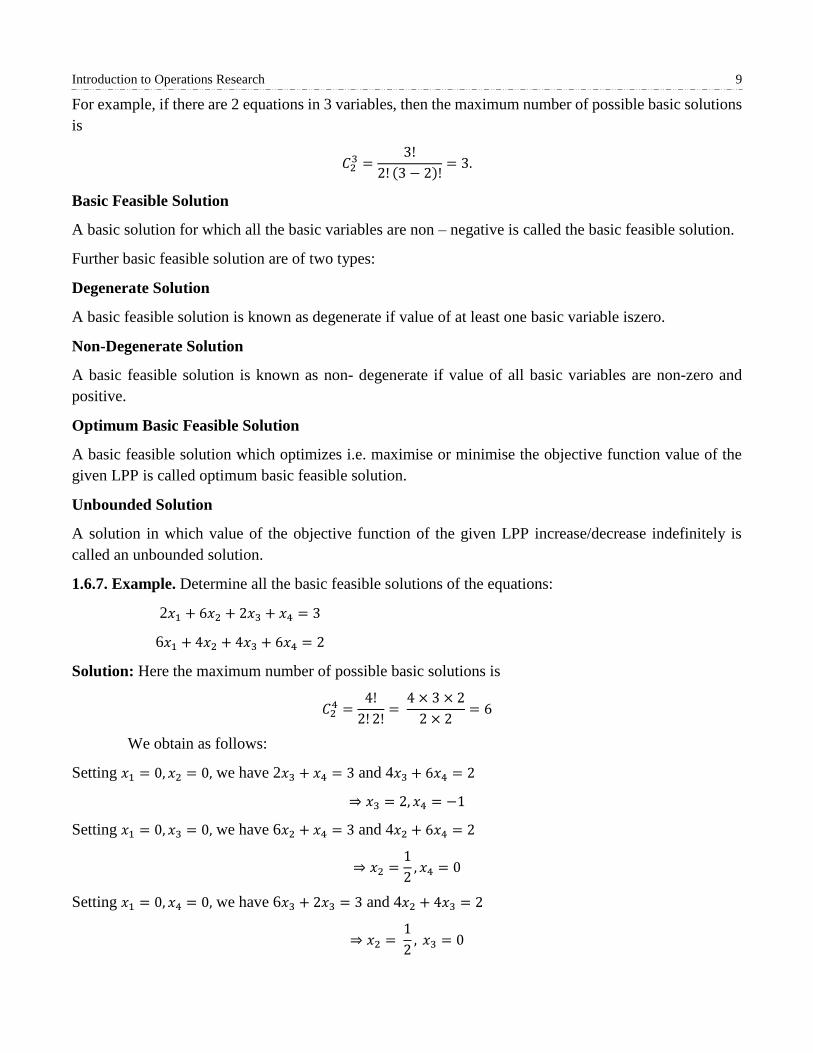
1.6.7. Example. Determine all the basic feasible solutions of the equations:
2𝑥1 + 6𝑥2 + 2𝑥3 + 𝑥4 = 3
6𝑥1 + 4𝑥2 + 4𝑥3 + 6𝑥4 = 2
Solution: Here the maximum number of possible basic solutions is
𝐶24 =
4!
2! 2!=
4 × 3 × 2
2 × 2= 6
We obtain as follows:
Setting 𝑥1 = 0, 𝑥2 = 0, we have 2𝑥3 + 𝑥4 = 3 and 4𝑥3 + 6𝑥4 = 2
⇒ 𝑥3 = 2, 𝑥4 = −1
Setting 𝑥1 = 0, 𝑥3 = 0, we have 6𝑥2 + 𝑥4 = 3 and 4𝑥2 + 6𝑥4 = 2
⇒ 𝑥2 =1
2, 𝑥4 = 0
Setting 𝑥1 = 0, 𝑥4 = 0, we have 6𝑥3 + 2𝑥3 = 3 and 4𝑥2 + 4𝑥3 = 2
⇒ 𝑥2 = 1
2, 𝑥3 = 0

10 Operations Research Techniques
Setting 𝑥2 = 0, 𝑥3 = 0, we have 2𝑥1 + 𝑥4 = 3 and 6𝑥1 + 6𝑥4 = 2
⇒ 𝑥1 =8
3, 𝑥4 = −
7
3
Setting 𝑥2 = 0, 𝑥4 = 0, we have 2𝑥1 + 2𝑥3 = 3 and 6𝑥1 + 4𝑥4 = 2
⇒ 𝑥1 = −2, 𝑥4 =7
2
Setting 𝑥3 = 0, 𝑥4 = 0, we have 2𝑥1 + 6𝑥2 = 3 and 6𝑥1 + 4𝑥2 = 2
⇒ 𝑥1 = 0, 𝑥2 =1
2
Thus, all basic solutions of the given system of equations are;
(0, 0, 2, -1), (0, 1
2, 0, 0), (0,
1
2, 0, 0) , (
8
3, 0, 0, −
7
3) , (−2, 0,
7
2, 0) , (0,
1
2, 0, 0).
Here (0,1
2, 0, 0) is repeated thrice and hence the basic solutions are
(0, 0, 2, -1),(0,1
2, 0, 0) , (
8
3, 0, 0, −
7
3) , (−2, 0,
7
2, 0).
Of these solutions, the basic feasible solution is (0,1
2, 0, 0) as in the other solutions, all decision variables
are not positive.
1.6.8. Exercises.
1 Find all basic solutions for the system of simultaneous equations:
2𝑥1 + 3𝑥2 + 4𝑥3 = 5 and 3𝑥1 + 4𝑥2 + 5𝑥3 = 6.
(Hint. The maximum number of possible basic solutions is
𝐶23 =
3!
2! (3 − 2)!= 3.
And no feasible solution)
2 Determine all the basic feasible solutions of the system of equations:
3𝑥1 + 5𝑥2 + 𝑥3 = 15and 5𝑥1 + 2𝑥2 + 𝑥4 = 10.
Further, discuss that whether the solution is degenerate or non-degenerate.
(Hint. The maximum number of possible basic solutions will be C24 =
4!
2!2!=
4×3×2
2×2= 6.
And the possible solutions are
(0, 0, 15, 10), (0, 3, 0, 4), (0, 5, -10, 0), (5, 0, 0, -15), (2, 0, 9, 0) and (50
19 ,
45
19 , 0, 0).)

Introduction to Operations Research 11
1.7. CHECK YOUR PROGRESS
1 Explain the concept and scope of Operations Research.
2 Explain the advantages and disadvantages of Operations Research.
3 Define the followings:
(i) Feasible solution
(ii) Degenerate solution
(iii) Extreme points of a convex set.
1.8. SUMMARY
In this chapter, we have introduced Operations Research, its scope, advantages and limitations. We have
observed that Operations Research is a very powerful method of getting the best out of limited resources.
It finds applications in almost every field. Here, we explain concept of convex sets which is another
important concept. We study feasible solution, basic solution, and basic feasible solution of a system of
equations less in number than the number of decision variables. Such solutions are required to be obtained
for finding out optimal solution of the given LPP.

2 LINEAR PROGRAMMING PROBLEMS
Structure
2.1. Introduction
2.2. Linear Programming Problem (LPP)
2.3. Mathematical Formulation of LPP
2.4. Graphical Method
2.5. Canonical and Standard Form of LPP
2.6. Check Your Progress.
2.7. Summary
2.1. INTRODUCTION
In 1947, George Dantzig and his associates, while working with the US Air Force during World War II,
developed this technique, primarily for solving military logistics problems. They observed that a large
number of military programming/planning problems could be formulated as maximizing/minimizing a
linear form of profit/cost function whose variable were restricted to values satisfying a system of linear
constraints. In chapter 1, We have already discussed the concept of optimization and explained the basic
feasible solution of linear programming problem.
In this chapter, we study linear programming problems (LPP), their mathematical formulation, objective
function concept and graphical method. We use graphical method mainly for solving problems involving
two variables. Linear programming can be applied to a variety of problems such as production,
transportation, advertising and problems in public and private organizations, e.g., business, industry,

Simplex Method and Duality in Linear Programming 13
hospitals, libraries as also in education. In order to solve linear programming problems, we need to convert
them into a canonical or standard form.
2.1.1. Objectives. The objective of these contents is to provide some important concepts/results to the
reader like:
Linear programming problems, it’s applications and limitations.
Mathematical formulation of linear programming problem.
Graphical Method
Canonical and Standard form of an LPP
2.2. LINEAR PROGRAMMING PROBLEM (LPP)
We have already familiar with the concept of optimization. A mathematical programming is an
optimization technique by which the maximum or minimum value of a function is determined under
certain conditions. Mathematical programming in which constraints are expressed as linear equalities /
inequalities is called linear programming.
We first introduce three basic components essential for the development of LP theory.
Decision Variables: The variables in terms of which the problem is defined.
Objective Function: A function which is to be maximised or minimised subject to the given
constraints/limitations.
Constraints: There are always certain limitations on the use of resources that limit the degree to which
an objective can be achieved. These limitations are known as constraints or restrictions. Constraints must
be represented as linear equalities or inequalities in terms of decision variables.
Every organisation, big or small wants to find the best allocation of resources in order to optimize the
objective function. We can use linear programming only if the following conditions are satisfied:
i. Objective function should be well defined
ii. Objective function can be expressed as a linear function of the decision variables.
iii. There should be finite number of constraints and can be expressed as linear equalities or
inequalities in terms of variables.
iv. Decision variables should be non- negative.
2.2.1. Advantages and Limitations of an LPP
Linear programming methods are used in many fields including business and industry by almost all their
departments such as production, marketing, finance etc. it’s some advantages are
Helps in attaining the optimum use of resources i.e. maximise profit and minimise costs
Improve the quality of decisions
There are many more advantages. In spite of having many advantages and wide areas of applications,
there are some limitations as well. Following are certain limitations of linear programming:
We can apply linear programming method only if relationships are linear.

14 Operations Research Techniques
While solving LPP, it is possible that we will get non-integral values even for those decision
variables which have only integral values.
Constraints in the linear programming methods are written assuming all parameters are known and
should be constant. However, in real problems, sometimes these are neither known nor constant.
LP deals with the problems having single objective, whereas in real-life, there are many situations
where we have to achieve multi-objectives.
2.3. MATHEMATICAL FORMULATION OF LPP
In our daily life, there are many real-life situations where LP problems may arise and for using LPP
methods/techniques to find a solution of such situations, it becomes necessary to present the given word
problem into mathematical form correctly. The steps of mathematical formulation of LPP are summarized
as follows:
i) Identify the decision variable of the given problem.
ii) Formulate the objective function, which is to be maximised or minimised, as a linear function of
the decision variables.
iii) Formulate the constraints and express them as linear inequalities or equalities in terms of decision
variables.
iv) Introduce non-negative restrictions as negative values of the decision variables do not have any
valid physical interpretation.
The steps of mathematical formulation of LPP are explained with the help of an example.
2.3.1. Example. A small-scale industry manufactures two products P and Q which are processed in
a machine shop and assembly shop. Product P requires 2 hours of work in a machine shop and 4
hours of work in the assembly shop to manufacture while product Q requires 3 hours of work in
the machine shop and 2 hours of work in the assembly shop. In one day, the industry cannot use
more than 16 hours of machine shop and 22 hours of assembly shop. It earns a profit of rupees 3
per unit of product P and rupees. 4 per unit of product Q. Give a mathematical formulation of the
problem as to maximise profit.
Solution: let x and y be the number of units of product P and Q, which are to be produced. Here x and y
are the decision variables. Suppose Z is the profit function.
Since one unit of product P and one unit of product Q gives the profit of rupees 3 and rupees 4,
respectively, the objective function is
Maximize Z =3x +4y
The requirement and availability in hours of each of the shops for manufacturing the products are tabulated
as follows:
Machine Shop Assembly Shop Profit
Product P 2 hours 4 hours Rs.3 per unit
Product Q 3 hours 2 hours Rs.4 per unit
Available hours per day 16 hours 22 hours

Simplex Method and Duality in Linear Programming 15
Total hours of machine shop required for both types of product = 2x+3y
Total hours of assembly shop required for both types of product =4x+2y
Hence, the constraints as per the limited available resources are:
2x+3y ≤ 16 and 4x+2y ≤ 22
Since the number of units produced for both P and Q cannot be negative, the non-negative restrictions are:
x ≥ 0, y ≥ 0
Thus, the mathematical formulation of the given problem is:
Maximise Z = 3x + 4y
Subject to the constraints
2x + 3y ≤ 16
4x + 2y ≤ 22
And non-negative restrictions
x ≥ 0, y ≥ 0
2.3.2. Exercise. A company produces two types of items P and Q that require gold and silver. Each
unit pf type P requires 4g silver and 1g gold while that od type Q requires 1g silver and 3g gold. The
company produces 8g silver and 9g gold. If each unit of type P brings a profit of rupees 44 and that
of type Q rupees 55, determine the number of units of each type that the company should produce
to maximise the profit.
Answer. Let Z be the profit function. The mathematical formulation of the given problem is
Max. Z = 44x + 55y
Subject to the constraints:
4x + y ≤ 8,
x + 3y ≤ 9, x ≥ 0, y ≥ 0.
2.4. GRAPHICAL METHOD
The graphical method is used to solve simple linear programming problems having two decision variables.
For solving LPPs involving more than two decision variables, we use another method called simplex
method. We discuss it in chapter 3.
The steps of graphical method for solving an LPP are as follows:
1. Plot the graph corresponding to the given constraints.
2. Determine the region for each given constraint.
3. Determine the feasible region.
4. Determine corner/extreme points.
5. Examine corner/extreme points.

16 Operations Research Techniques
The following example explains steps of Graphical method.
2.4.1. Example.
The graphs are plotted for the equalities corresponding to the given inequalities for constraints as well as
restrictions. That is, we first draw the straight lines. For example, suppose one of the given inequalities is
2x+3y ≤ 6. Then, we first plot the graph for the equation 2x+3y = 6, which is straight line. For this, we
take any two points on it join them.
For example, for x = 0, y = 6/3 = 2 and for y = 0, x = 6/2 = 3. So, we get the straight line shown in fig.
2.1.
Fig.2.1
First, we determine the region corresponding to each inequality. Let us consider the inequality 2x+3y ≤ 6
again. We can find the region on the graph satisfied by this inequality by substituting x = 0 and y = 0 in
it. We get
2(0) + 3(0) ≤ 6 => 0 ≤ 6
which is correct. So, it is the region containing the point (0, 0). Hence, half plane shown in Fig. 2.2 by
shading the region starting from the line towards the point (0, 0) is the graph of the given inequality.
Fig.2.2

Simplex Method and Duality in Linear Programming 17
Had the given inequality been 2x+3y≥6, then we would have shaded the region on the opposite side of the
line. This is because on putting x=0, y=0 in the inequality, we get
2(0) + 3(0) ≥ 6 => 0≥6
which is not correct. Thus, the point (0, 0) does not satisfy the inequality and hence does not lie in the
region. Thus, graph for the inequality 2x-3y ≥ 6 would, therefore, be as shown in Fig. 2.3.
Fig.2.3
In this example, we have used the point (0, 0) to determine which half plane corresponds to the given
inequality. However, you can take any other point. But using (0, 0) is far easier. If the right-hand side of
the given inequality is zero, using the point (0, 0) in it is meaningless. For example, suppose the given
inequality is 2x-3y≥0.The plot of 2x-3y=0 is given in fig. 2.4. It is straight line passing through the origin.
Using the point (0, 0) in the inequality 2x-3y ≥ 0, we get 2(0)-3(0) ≥ 0, i.e., 0 ≥ 0. So, we cannot decide
which half plane is the region of the given inequality. Therefore, in this case, we use any other point, say
(2, 0), on putting x=2, y=0 in the given inequality, we get
2(2)-3(0) ≥ 0 and 4 ≥ 0
which is true. Therefore, the half plane containing (2, 0) is the required region as shown in Fig.2.4.
2x-3y=0 or 3y=2x or y=2x/3
Fig.2.4

18 Operations Research Techniques
After determining the regions for each inequality, we find their common region. This is the region where
all the given inequalities and non-negative restrictions are satisfied. This common region is known as
feasible region or the solution set or polygonal convex set.
Now, we determine each of the corner points (vertices) of the polygon obtained in step 3. This is done
either by plotting graphs on graph paper or by solving the two equations of the lines intersecting at that
point.
Evaluate the value of the objective function at each corner point and determine the extreme point of the
feasible region that has optimum objective function value.
According to the feasible region, we have different types of solution.
a) If the feasible region is bounded. The maximum of the values obtained for the objective function at the
corner points is the optimum value when the objective function is of maximization form. The point
corresponding to this maximum value give the required values of the decision variables. The minimum
of the values obtained for the objective function at the corner points is the optimum value when the
objective function is of minimization form. The point corresponding to this minimum value give the
required values of the decision variables.
b) If the feasible region is not bounded. Then either there are additional hidden conditions which can be
used to bound the region or there is no solution to the problem.
c) If the same optimum value exists at two of the vertices, then there are multiple solutions to the problem.
Suppose these are two points (𝑥1 , 𝑦1) and (𝑥2 , 𝑦2). Then other solutions are given by the point as follow:
[First ordinate of first point × t + First ordinate of second point × (1- t ) ,
Second ordinate of first point × t + Second ordinate of second point × (1 – t)]
where t is any real number lying between 0 and 1.
For example, let the objective function be Z = 3x – y and let A (2,1) and B (3,4) be the points which give
the same optimum value of the objective function, i.e., Z = 5. Then other solutions which give the same
value of the objective function are:
(2 × t + 3 × (1 – t), 1 × t + 4 × (1 – t))
Or (2t + 3 – 3t, t + 4 – 4t)
Or (3 – t, 4 – 3t), 0 ≤ t ≤ 1
Here t = 0 gives the point (3, 4), which is the point B and t = 1 gives the point (2, 1), which is the point A.
The real values of t between 0 and 1 give other points which give the same optimum solution. One such
point other than A and B is
( 3 - 1
2 , 4 – 3 ×
1
2 ) , t =
1
2 , i.e. , (
5
2 ,
5
2 )
You can verify that Z = 5 at the point ( 5
2 ,
5
2 ) .
2.4.2. Example. A company produces two types of items P and Q that require gold and silver. Each
unit pf type P requires 4g silver and 1g gold while that od type Q requires 1g silver and 3g gold. The
company produces 8g silver and 9g gold. If each unit of type P brings a profit of rupees 44 and that

Simplex Method and Duality in Linear Programming 19
of type Q rupees 55, determine the number of units pf each type that the company should produce
to maximise the profit. What is the maximum profit?
Solution. Let x be the number of units of type P to be produced and y be the number of units of type Q to
be produced. It is given that:
Silver Gold Profit
Type P 4g 1g Rs.44 per unit
Type Q 1g 3g Rs.55 per unit
Available (at the
most)
8g 9g
Let Z be the profit function. The mathematical formulation of the given problem is
Max. Z = 44x + 55y
Subject to the constraints:
4x + y ≤ 8,
x + 3y ≤ 9,
x ≥ 0, y ≥ 0.
First of all, we plot the graphs for the equations:
4x + y = 8, x + 3y = 9 , x = 0 , y = 0 .
Since these equations are of straight lines, only two points are sufficient to plot the graphs ( see fig.2.5).
For the line 4x + y = 8, we take the following two points:
X 0 2
Y 8 0
Similarly, for the line x + 3y = 9, we take
X 0 9
Y 3 0
Now, plotting the above lines, we get fig.2.5.

20 Operations Research Techniques
Fig.2.5
Note that x = 0 is the y axis and y = 0 is the x axis.
For plotting the graph of the inequality 4x + y ≤ 8 we put (0, 0) In it. We get 0 ≤ 8, which is true. Therefore,
starting from the line 4x + y ≤ 8, we shall shade towards origin. Similarly, for the graph x + 3y ≤ 9, we
shall shade towards origin. For the graph x ≥ 0. we shall shade towards right side of x = 0 and for the
graph y ≥ 0, the region above y = 0 will be shaded.
Thus, the regions for the inequalities are shown in fig.2.6.
Fig.2.6.
You can see from the figure 2.6 that the coordinates of A, B, and D are (0, 0), (2, 0) and (0,3) respectively.
The coordinates of the point C are obtained by solving the equations 4x + y = 8 and x + 3y = 9 as it is the
point of intersection of the two lines represented by them. the solution of equations 4x + y = 8 and x + 3y
= 9 is given as

Simplex Method and Duality in Linear Programming 21
x = 15
11 and y =
28
11
So the vertices of ABCD are A(0,0) , B(2,0) , C(15
11 ,
28
11 ) and D (0,3).
We now obtain the values of Z = 44x + 55y at each of the vertices of ABCD as follows:
At A (0,0) , Z = 44(0) + 55(0) = 0
At B(2,0) , Z = 44(2) + 55(0) = 88
At C(15
11 ,
28
11 ) , Z = 44(
15
11) + 55(
28
11) = 60 + 140 = 200
At D (0,3), Z = 44(0) + 55(3) = 165
Thus, the value of Z is maximum at C (15
11 ,
28
11 ) and the optimum solution is Max.Z = 200 when x =
15
11 and
y = 28
11 .
2.4.3. Exercises.
1. Maximise Z = 6X + 3Y subjects to the constraints
2X + 5Y ≤ 120, 4X + 2Y ≤ 80, X ≥ 0 , Y ≥ 0.
2. Maximise z = 3𝐱𝟏 + 2𝐱𝟐 subjects to the constraints
𝐱𝟏- 𝐱𝟐 ≤ 1, 𝐱𝟏+ 𝐱𝟐 ≥ 3,𝐱𝟏≥ 0 , 𝐱𝟐 ≥ 0
3. Maximise Z = 𝐱𝟏+ 𝐱𝟐 subjects to the constraints
𝐱𝟏+ 𝐱𝟐 ≤ 1, 3𝐱𝟏+ 𝐱𝟐 ≥ 3, 𝐱𝟏≥ 0 , 𝐱𝟐 ≥ 0
4. A company manufactures two products X and Y, each of which requires three types of
processing. The length of time for processing each unit and the profit per unit are given in
the following table:
Product X (hr/unit) Product Y (hr/unit) Available capacity
per day (hr)
Process 1 12 12 840
Process 2 3 6 300
Process 3 8 4 480
Profit per unit 5 7
How many units of each product should the company manufacture per day in order to
maximise profit?
5. A company produces soft drinks and has a contract requiring that a minimum of 80 units of
chemical A and 60 units of chemical B go into each bottle of the drink. The chemicals are
available in a prepared mix from two different suppliers. The supplier X1 has a mix of 4 units
of A and 2 units of B that costs rupees 10, and the supplier X2 has a mix of 1 unit of A and 1
unit of B that costs rupees 4. How many mixes from the company X1 and company X2 should
the company purchase to honour contract requirement and yet minimise cost?

22 Operations Research Techniques
2.5. CANONICAL AND STANDARD FORM OF AN LPP
After formulating a linear programming problem, our next step is to solve it. You have learnt that linear
programming problems can be represented as problems of maximisation or minimisation with constraints
such as ≤ , =, ≥ . In order to develop a standard procedure for solving LPPs, we need to convert them into
well - known form. We now discuss the General LPP along with these two forms. The canonical form is
especially used in the duality theory and the standard form is used to develop the general procedure for
solving any linear programming problem. In order to understand these forms, you also need to learn about
slack and surplus variable.
2.5.1. General Linear Programming Problem
Let us formulate the general linear programming problem. Let Z be a linear function of n basic variables
𝑋1,𝑋2, 𝑋3,..., 𝑋𝑛, which is to be maximised (or minimised). We write the problem as
Maximise (or minimise) Z = 𝐶1𝑋1 + 𝐶2𝑋2 + 𝐶3𝑋3 + ... +𝐶𝑛𝑋𝑛.... (1)
where 𝐶1, 𝐶2, 𝐶3, ... , 𝐶𝑛 are known constant termed as cost coefficients of basic variables.
Let (𝑎𝑖𝑗) be an m×n real matrix of m×n constants 𝑎𝑖𝑗’s and let {𝑏1,, 𝑏2, … , 𝑏𝑚} be a set of constants such
that
𝑎11𝑥1 + 𝑎12𝑥2 + ... + 𝑎1𝑛𝑥𝑛 ≤ or = or , ≥ 𝑏1
𝑎21𝑥1 + 𝑎22𝑥2 + ... + 𝑎2𝑛𝑥𝑛 ≤ or = or , ≥ 𝑏2
. . . . .... (2)
. . . .
. . . .
𝑎𝑚1𝑥1 + 𝑎𝑚2𝑥2 + ... + 𝑎𝑚𝑛𝑥𝑛 ≤ or = or, ≥ 𝑏𝑚
and 𝑥𝑗≥ 0 for all j = 1 ,2, 3, ..., n ... (3)
The linear function Z in equation (1) is called the objective function. The set of inequalities given in (2)
is called constraints of a general LPP and the set of inequalities given in (3) are known as non – negative
restrictions of a general LPP.
2.5.2. Slack and Surplus Variables
In general, if any linear programming problem, we have a constraint of the type
𝑎11𝑥1 + 𝑎12𝑥2 + ... + 𝑎1𝑛𝑥𝑛 ≤ 𝑏1 where 𝑏1≥ 0
Then this inequality can be converted into an equation by adding one non – negative variable 𝑠1 to the
left-hand side. This new variable is called a slack variable and the constraints are transformed into the
following equation:
𝑎11𝑥1 + 𝑎12𝑥2 + ... + 𝑎1𝑛𝑥𝑛 + 𝑠1 = 𝑏1 where 𝑠1≥ 0, 𝑏1≥ 0
Thus, a non – negative variable subtracted from the left – hand side of less than or equal to (≤) type of a
constraint that converts it into an equation is called a slack variable. The values of this

Simplex Method and Duality in Linear Programming 23
variable can be interpreted as the amount of unused resource.
Similarly, if in any linear programming problem, we have a constraint of the type
𝑎11𝑥1 + 𝑎12𝑥2 + ... + 𝑎1𝑛𝑥𝑛≥ 𝑏1
Then this inequality can be converted into an equation by subtracting one non –negative variable 𝑠1 from
the left-hand side. This new variable is called a surplus variable. The value if this variable can be
interpreted as the amount over and above the required minimum level.
Canonical Form
The characteristics of the canonical form are:
(a). Objective function should be of maximization form. If it is given in minimization form, it should be
converted into maximization form.
(b). All the constraints should be of “≤ ” type, except for non- negative restrictions. Inequality of “ ≥ ”
type, if any, should be changed to an inequality of the “ ≤ ” type.
(c). All variables should be non-negative. If a given variable is unrestricted in sign (i.e., positive, negative
or zero), it can be written as a difference of two non-negative variables. Suppose x is unrestricted in sign,
then x can be written as x= 𝑥′- 𝑥′′ where 𝑥′ ≥ 0, 𝑥′′ ≥ 0.
2.5.3. Example. Express the following LPP in Canonical form:
Minimize Z = 2𝑥1 + 𝑥2 + 4𝑥3
Subject to the constraints:
- 2𝑥1 + 4𝑥2≤ 4
𝑥1 + 2𝑥2 + 𝑥3 ≥ 5
2𝑥1 + 3𝑥3≤ 2
𝑥1,𝑥2 ≥ 0 and 𝑥3 is unrestricted in sign
Solution: Here, the objective function is of the minimisation form. We rewrite it in the maximisation form
as follows:
Minimise Z = 2𝑥1 + 𝑥2 + 4𝑥3
Thus, we have to maximise -Z = -2𝑥1 - 𝑥2 - 4𝑥3. So the problem becomes,
Maximise 𝑍′= -2𝑥1 - 𝑥2 - 4𝑥3. where 𝑍′ = -Z
Now the second constraints is of the type “≥”. Hence to convert it into type “≤”, we multiply the inequality
by -1 and write
- 𝑥1 - 2𝑥2 - 𝑥3≤ -5
Other constraints are already in the desired form. But 𝑥3is unrestricted in sign. So, we write
𝑥3 = 𝑥3′ − 𝑥3
′′ , where 𝑥3′ ≥ 0, 𝑥3
′′≥ 0.
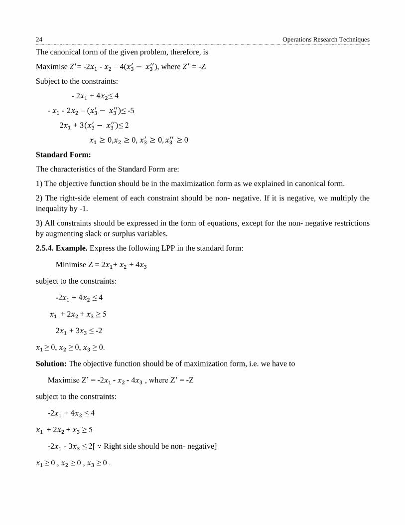
24 Operations Research Techniques
The canonical form of the given problem, therefore, is
Maximise 𝑍′= -2𝑥1 - 𝑥2 – 4(𝑥3′ − 𝑥3
′′), where 𝑍′ = -Z
Subject to the constraints:
- 2𝑥1 + 4𝑥2≤ 4
- 𝑥1 - 2𝑥2 – (𝑥3′ − 𝑥3
′′)≤ -5
2𝑥1 + 3(𝑥3′ − 𝑥3
′′)≤ 2
𝑥1 ≥ 0,𝑥2 ≥ 0, 𝑥3′ ≥ 0, 𝑥3
′′ ≥ 0
Standard Form:
The characteristics of the Standard Form are:
1) The objective function should be in the maximization form as we explained in canonical form.
2) The right-side element of each constraint should be non- negative. If it is negative, we multiply the
inequality by -1.
3) All constraints should be expressed in the form of equations, except for the non- negative restrictions
by augmenting slack or surplus variables.
2.5.4. Example. Express the following LPP in the standard form:
Minimise Z = 2𝑥1+ 𝑥2 + 4𝑥3
subject to the constraints:
-2𝑥1 + 4𝑥2 ≤ 4
𝑥1 + 2𝑥2 + 𝑥3 ≥ 5
2𝑥1 + 3𝑥3 ≤ -2
𝑥1 ≥ 0, 𝑥2 ≥ 0, 𝑥3 ≥ 0.
Solution: The objective function should be of maximization form, i.e. we have to
Maximise Z’ = -2𝑥1 - 𝑥2 - 4𝑥3 , where Z’ = -Z
subject to the constraints:
-2𝑥1 + 4𝑥2 ≤ 4
𝑥1 + 2𝑥2 + 𝑥3 ≥ 5
-2𝑥1 - 3𝑥3 ≤ 2[ ∵ Right side should be non- negative]
𝑥1 ≥ 0 , 𝑥2 ≥ 0 , 𝑥3 ≥ 0 .

Simplex Method and Duality in Linear Programming 25
Now the inequalities are to be converted to equations. Note that the first and third inequalities are of the
type “less than or equal to (≤)”.
Therefore, a slack variable is to be added to the left side of each of these inequalities. The second inequality
is of the type “more than or equal to (≥) ” . So, a surplus variable is to be subtracted from the left side of
this inequality.
Thus, a standard form of the given LPP is
Max.Z’ = = -2𝑥1 - 𝑥2 - 4𝑥3 + 0𝑠1 + 0𝑠2 + 0𝑠3 , where Z’ = -Z
subject to the constraints:
-2𝑥1 + 4𝑥2 + 𝑠1 = 4
𝑥1 + 2𝑥2 + 𝑥3 - 𝑠2 = 5
-2𝑥1 - 3𝑥3 + 𝑠3 = 2
𝑥1 ≥ 0 , 𝑥2 ≥ 0 , 𝑥3 ≥ 0 , 𝑠1 ≥ 0 , 𝑠2 ≥ 0 , 𝑠3 ≥ 0 .
2.5.5. Exercise.
1. Express the following LPP in
(i) Canonical form
(ii) Standard Form
Minimise Z = 𝑥1 - 2𝑥2 + 𝑥3
subjects to the constraints:
2𝑥1 + 3𝑥2 + 4𝑥3 ≥ -4
3𝑥1 + 5𝑥2+ 2𝑥3 ≥ 7
𝑥1 ≥ 0 , 𝑥2 ≥ 0 , 𝑥3 ≥ 0 .
2. Max. Z = 5x + 7y
subjects to the constraints:
12x + 12y ≤ 840 => x + y ≤ 70
3x + 6y ≤ 300 => x + 2y ≤ 100
8x + 4y ≤ 480 => 2x + y ≤ 120
x ≥ 0 , y ≥ 0

26 Operations Research Techniques
Answer.
Fig.2.8.
The maximum value of Z is 410 at C(40,30) , i.e., at x = 40 , y = 30.
3. Minimise z = 10𝑥1 + 4𝑥2
subjects to the constraints
4𝑥1 + 𝑥2 ≥ 80
2𝑥1 + 𝑥2≥ 60
𝑥1≥ 0 , 𝑥2 ≥ 0
Answer.
Fig.2.9.

Simplex Method and Duality in Linear Programming 27
The maximum value of Z is 260 at B (10,40), i.e. 𝑥1 = 10 and 𝑥2 = 40.
Note: Had the objective function been of maximization form, the problem would have the unbounded
solution. This is because the values of 𝑥1 and 𝑥2 could be increased beyond any limit, which would result
in higher value of Z with no upper bound.
2.6. CHECK YOUR PROGRESS
1. What is linear programming? What are its major advantages and limitations?
2. What is meant by feasible solution of an LP problem?
2.7. SUMMARY
In this chapter, we introduced the concept of LPP and explain how these are formulated mathematically.
We define objective function and graphical method of obtaining optimum value which is used to solve
linear programming problems having two decision variables. Here, we study about feasible region/
solution set in detail. Also, we discuss canonical and standard form of an LPP as to solve LPP we need to
convert them into a canonical or standard form.

3 SIMPLEX METHOD AND DUALITY IN LINEAR PROGRAMMING
Structure
3.1. Introduction
3.2. Simplex Method
3.3. Artificial Variable Techniques
3.4. Big-M Method
3.5. Two-Phase Method
3.6. Degeneracy
3.7. Duality in Linear Programming
3.8. Check Your Progress
3.9. Summary
3.1. INTRODUCTION
In chapter 2, we have studied the graphical method of solving linear programming problems and learnt
how to express a linear programming problem in canonical and standard forms. As we know that the
graphical method can be used only to solve the problems involving two decision variables and most of the
real-life problems when mathematically formulated have more than two variables. For more than two
decision variables, methods based on the concept of slack or surplus variables are used.

Simplex Method and Duality in Linear Programming 29
In this chapter, first we shall discuss the Simplex method for solving the linear programming problems
involving more than two decision variables. After learning the procedure of simplex method, we discuss
artificial variable techniques (Big-M Method and Two-Phase Method) for solving LPP and in last we shall
discuss the concept of degeneracy in linear programming.
3.1.1. Objectives. The objective of these contents is to provide some important concepts/methods to the
reader like:
Simplex Method.
Artificial Variable Techniques.
Big-M and Two-Phase Method for Solving LPP Involving Artificial Variable(s).
Degeneracy.
3.2. SIMPLEX METHOD
Simplex method was developed by G B Dantzig in 1947. The method is an iterative or step by step
procedure by which one can obtained a new basic feasible solution from a given initial basic feasible
solution. In this method, the value of the objective function improves with each solution and the
optimum solution is achieved in a finite number of steps.
Suppose we have to optimize (maximiseor minimise) Z, a linear function of n basic variables
𝑋1, 𝑋2, … , 𝑋𝑛. The LPP is written as:
Maximise Z = 𝐶1𝑋1 + 𝐶2𝑋2 + ⋯ + 𝐶𝑛𝑋𝑛 … (1)
subject to the constraints:
𝑎11𝑥1 + 𝑎12𝑥2 + ⋯ + 𝑎1𝑛𝑥𝑛 ≤ 𝑏1
𝑎21𝑥1 + 𝑎22𝑥2 + ⋯ + 𝑎2𝑛𝑥𝑛 ≤ 𝑏2
∙ ∙ ∙ ∙ (2)
∙ ∙ ∙ ∙
𝑎𝑚1𝑥1 + 𝑎𝑚2𝑥2 + ⋯ + 𝑎𝑚𝑛𝑥𝑛 ≤ 𝑏𝑚
and 𝑥𝑗 ≥ 0 for all j= 1,2, …, n … (3)
where the constants 𝐶1, 𝐶2, … , 𝐶𝑛 are the cost coefficients of decision variables. Let (𝑎𝑖𝑗) be m×n real
matrix and {𝑏1, 𝑏2 , … , 𝑏𝑚} be a set of constants.
The linear function Z gives in equation (1) is called the objective function. The set of inequalities gives in
equation (2) is called constraints of LPP and the inequalities gives in equation (3) are known as non-
negative restrictions of LPP (which means that all 𝑥𝑗 values are non –negative)
Let us explain the step by step procedure for solving the LPP by the Simplex method.
Step 1: Convert the LPP into standard form by adding slack variables
We convert the given LPP into standard form by adding slack variables 𝑠1, 𝑠2, … , 𝑠𝑚.

30 Operations Research Techniques
Maximise Z = 𝐶1𝑋1 + 𝐶2𝑋2 + ⋯ + 𝐶𝑛𝑋𝑛 + 0𝑠1 + 0𝑠2 + ⋯ + 0𝑠𝑚 … (4)
subject to the given constraints:
𝑎11𝑥1 + 𝑎12𝑥2 + ⋯ + 𝑎1𝑛𝑥𝑛 + 𝑠1 = 𝑏1
𝑎21𝑥1 + 𝑎22𝑥2 + ⋯ + 𝑎2𝑛𝑥𝑛 + 𝑠2 = 𝑏2
∙ ∙ ∙ ∙ … (5)
∙ ∙ ∙ ∙
𝑎𝑚1𝑥1 + 𝑎𝑚2𝑥2 + ⋯ + 𝑎𝑚𝑛𝑥𝑛 + 𝑠𝑚 = 𝑏𝑚
and 𝑥𝑗 ≥ 0 𝑎𝑛𝑑 𝑠𝑖 ≥ 0 for all i =1, 2,…, m and j= 1,2, …, n … (6)
Step 2: Construct the initial simplex table.
The initial simplex table is formed as follows:
𝑪𝒋 → 𝑪𝟏 𝑪𝟐 . . 𝑪𝒓 0 0…
Basic
variables
Profit/unit
(𝑪𝑩)
Quantity 𝑋1 𝑋2 . . 𝑋𝑟 𝑆1 𝑆2.. Replacement
Ratios
𝑆1
𝑆2
.
.
.
0
0
.
.
.
𝑏1
𝑏2
.
.
.
𝑎11
𝑎21
.
.
.
𝑎12
𝑎22
.
.
.
. . 𝑎1𝑟
. . 𝑎2𝑟
.
.
.
1
0
.
.
.
0..
1..
.
.
.
𝑧𝑗 →
Z
𝑐𝑗 − 𝑧𝑗 →
𝑪𝑩𝑿𝟏 𝑪𝑩𝑿𝟐 . . 𝑪𝑩𝑿𝒓 𝑪𝑩𝑺𝟏 𝑪𝑩𝑺𝟐
Table 1: Initial Simplex Table
Step 3: Test for optimality
Calculate the values of 𝑐𝑗 − 𝑧𝑗 , the nature of the solution could be any one of the following:
1. If all 𝑐𝑗 − 𝑧𝑗 ≤ 0, the solution under test is optimal solution.
2. If at least one value of 𝑐𝑗 − 𝑧𝑗is positive and corresponding to the most positive
𝑐𝑗 − 𝑧𝑗 ,all the elements of the column 𝑋𝑗are negative or zero, the solution under test is an
unbounded solution.
3. Suppose at least one value of 𝑐𝑗 − 𝑧𝑗is positive. Suppose the most positive value is, say 𝑐3 − 𝑧3and
at least one entry in the column of 𝑋3 is positive. Then the solution under test is not optimal.

Simplex Method and Duality in Linear Programming 31
Step 4: Select incoming variable to enter the basis
If the solution is not optimal then we look for most positive entry and it could be any of (𝑐𝑗 − 𝑧𝑗). In this
case, we proceed as follows to obtain the optimal solution:
1. Let 𝑋𝑟 be the variable which corresponds to the most positive value of 𝑐𝑗 − 𝑧𝑗 . This variable is called
the incoming variable.
2. The column to be entered is called the key or pivot column.
Step 5: Test for feasibility (variable to leave the basis)
After finding the incoming variable, we determine the outgoing variable. For this we proceed as follow:
1. We divide the value of the Quantity (Qty) column be the corresponding positive values in the column
𝑋𝑟 . These ratios are called Replacement Ratios (RR). Note that we do not consider the negative
values in the column of 𝑋𝑟 for calculating RR. Then we select the minimum RR. The basic variable
corresponding to this value of the RR is called the outgoing variable. It is called outgoing variable
because it is removed (goes out) from the next simplex table. The row selected in this manner is
called key or pivot row.
2. The element that lies at the intersection of the key row and key column is called the key element or
leading element or pivot element.
Step 6: Finding the new solution
1. We convert the key element to unity by dividing all entries in the row by the key element itself.
2. In the next step, we would like that the values of all other elements in the column corresponding to key
element are zero. For this we carry out suitable operations on each row using the row containing the
key element.
Step 7: Repeat the procedure
Go to step 3 and repeat the procedure until all entries in the 𝑐𝑗 − 𝑧𝑗 are either negative or zero i.e. we
repeat the procedure until either an optimal solution is obtained or there is an indication of unbounded
solution.
The following example illustrate the simplex method:
3.2.1. Example. Maximise Z=3𝑥1 + 2𝑥2
subject to the constraints:
𝑥1 + 𝑥2 ≤ 4
𝑥1 − 𝑥2 ≤ 2
𝑥1 ≥ 0, 𝑥2 ≥ 0
Solution: Step 1: First we convert the given LPP into standard form by adding slack variables 𝑠1 and 𝑠2.
Maximize Z = 3𝑥1 + 2𝑥2 + 0𝑠1 + 0𝑠2
subject to the constraints:

32 Operations Research Techniques
𝑥1 + 𝑥2 + 𝑠1 = 4
𝑥1 − 𝑥2 + 𝑠2 = 2
𝑥1, 𝑥2, 𝑠1, 𝑠2 ≥ 0
Step 2: We now construct the initial simplex table (Table 2: Initial Simplex Table)
𝑐𝑗 → 3 2 0 0
Basic
variables
Profit/unit
(𝐶𝐵)
Quantity 𝑥1 𝑥2 𝑠1 𝑠2
𝑠1 0 4 1 1 1 0
𝑠2 0
2 1 -1
0
1
Z=
𝑧𝑗 →
𝑐𝑗 − 𝑧𝑗 →
Note: Columns corresponding to the basic variables in initial simplex tables in the simplex method form
an identity matrix. For example, in Table 2, the basic variables are 𝑠1 and 𝑠2 and their coefficients in the
constraints form identity matrix.
The value of Z in column of Table2 is obtained from the equation
Z=∑ 𝑐𝑗 𝑏𝑗, j=1, 2
The values of 𝑧𝑗′𝑠 are obtained from the equation
𝑧𝑗 = ∑ 𝑐𝑖𝑎𝑖𝑗𝑚𝑖=1 , where m is the number of rows. In this example m=2
Next, we obtain 𝑐𝑗 − 𝑧𝑗 , known as net-evaluations. These are 3,2,0,0.
Thus, the table takes the following form (Table3):
Table 3: Simplex Table
𝑐𝑗 → 3 2 0 0
Basic
variables
Profit/unit
(𝐶𝐵)
Quantity 𝑥1 𝑥2 𝑠1 𝑠2
𝑠1 0 4 1 1 1 0
𝑠2 0
2
1 -1
0
1
Z=0
𝑧𝑗 →
𝑐𝑗 − 𝑧𝑗 →
0
3
0
2
0
0
0
0

Simplex Method and Duality in Linear Programming 33
Step 3: Test for optimality
Since all 𝑐𝑗 − 𝑧𝑗 ≥ 0, therefore the current solution is not optimal.
Step 4: Now we select incoming and outgoing variable.
For this, we select the most positive value of 𝑐𝑗 − 𝑧𝑗 ,which is 3 in this case.
This corresponds to the variable 𝑥1 which becomes the incoming variable. We shall enter it as a basic
variable in the next simplex table.
Step 5: One of the variables 𝑠1, 𝑠2 will now be the outgoing variable which would be replaced by 𝑥1. To
find out which one of these variables (𝑠1𝑜𝑟 𝑠2) is the outgoing variable, we determine the replacement
ratio (RR). Recall that RR for any row is obtained by dividing the value of Quantity column by the
corresponding value of the Incoming variable for that particular row. For example, consider the first row
in Table 3. The value of Quantity in the first row is 4 and the value of the incoming variable 𝑥1 in this
row is 1.
Therefore, RR for the first row is 4
1 . For the second row, Quantity is 2 and value of 𝑥1 is 1. Hence, RR is
2
1 . RR is shown in the last column of the next simplex table (Table4).
The outgoing variable is the variable for which RR minimum. In Table 4, RR in the second row is
minimum. It corresponds to 𝑠2 and hence 𝑠2 is the outgoing variable.
The element which lies at the intersection of the column of incoming variable (𝑥1) and the row of the
outgoing variable (𝑠2) is called the key element. Here it is 1 and is enclosed by the rectangle as shown in
Table4. Incoming variable Key element
𝑐𝑗 → 3 2 0
𝑠1
0
Basic
variables
Profit/unit
(𝐶𝐵)
Quantity 𝑥1 𝑥2 𝑠2 R.R.
𝑠1 0 4 1 1 1 0 4/1=4
(outgoing
Variable)𝑠2
0
2
1 -1
0
1
2/1=2
Z=0
𝑧𝑗 →
𝑐𝑗 − 𝑧𝑗 →
0
3
0
2
0
0
0
0
The objective function Z=0 at 𝑥1 = 0 𝑎𝑛𝑑 𝑥2 = 0 (since 𝑥1 𝑎𝑛𝑑 𝑥2 do not appear in the column of basic
variables, these are non-basic variables. The values of non-basic variables are taken as zero). This is the
initial solution, which we shall improve.
Step 6: Now, we form the next simplex table to find the adjacent vertex, i.e., the improved solution. The
steps for forming this table are explained below:
1

34 Operations Research Techniques
a) The initial simplex table (Table 4) has revealed that 𝑥1 is an incoming variable which will enter in place
of 𝑠2, the outgoing variable. The cost coefficient of 𝑠2will also be replaced by the cost coefficient of 𝑥1
in “Profit / Unit” column. In this case its value is 3. Therefore, now the simplex table takes the form of
Table 5. Other entries of the table will be filled up as explained in point (b).
b) Since 𝑥1 has entered as a basic variable, the coefficients of 𝑥1 along with 𝑠1 should form an identity
matrix; i.e., the column corresponding to 𝑥1 should be (01). Thus, we have to make the key element
unity and the other element zero. Note that it is already unity in this case (Table 4). Had it been any
number other than unity, we would have divided the row containing leading element by the leading
element itself, excluding the elements of the column “Profit / Unit”. So, the table takes the form
Table 5: Simplex Table
𝑐𝑗 → 3 2 0 0
Basic
variables
Profit/unit (𝐶𝐵) Quantity 𝑥1 𝑥2 𝑠1 𝑠2
𝑠1 0 4 1 1 1 0
𝑥1 3
2
1 -1
0
1
c) Now, we have to make the other element in the column of key element (𝑥1 ) zero. In this case,
itsvalue is 1 (𝑎11 = 1). For this, we multiply the row of the key element (excluding profit / unit) by
negative of the element 𝑎11 (in this case) and add it to the first row.
This row operation is shown below:
First row of Table 7→ 4 1 1 1 0
Second row of Table 7→ -2 -1 1 0 -1
(on multiplying by -1)
Sum of the rows 2 0 2 1 -1
Thus, the sum of the rows is the new first row (excluding profit/ unit), which replaces the first row of
Table5. We get Table 6 as follows:
Table 6: Simplex Table
𝑐𝑗 → 3 2 0 0
Basic
variables
Profit/unit
(𝐶𝐵)
Quantity 𝑥1 𝑥2 𝑠1 𝑠2
𝑠1 0 2 0 2 1 -1
𝑥1 3 2
1 -1
0
1
Note: Now the matrix for the basic variables 𝑠1 and 𝑥1 in the Table 6 is the identity matrix.

Simplex Method and Duality in Linear Programming 35
d) Next, we calculate 𝑧𝑗 and 𝑐𝑗 − 𝑧𝑗. The resulting simplex table is given below:
Table 7: Simplex Table
𝑐𝑗 → 3 2 0
𝑠1
0
Basic
variabl
es
Profit/unit (𝐶𝐵) Quantity 𝑥1 𝑥2 𝑠2 RR
← 𝑠1 0 2 0 2 1 -1 2/2=1←
𝑥1 3
2
1 -1
0
1
-
Z=0× 2 + 3 ×2 = 6
𝑧𝑗 →
0 × 0+ 3 × 1= 3
0 × 2 + 3× (−1)= −3
0 × 1+ 3 × 0= 0
0× (−1)+ 3 × 1= 3
𝑐𝑗 − 𝑧𝑗
→
0 5
↑
0 -3
Here Z=6 at 𝑥1 = 2 (see the value in the Quantity column) and 𝑥2=0 (𝑥2 being non-basic variable).
In Table 7, the incoming variable is 𝑥2 corresponding to the most positive value of 𝑐𝑗 − 𝑧𝑗 = 5. The key
element is 2. We find the RR by dividing the elements in the Quantity column by the corresponding
elements in the column of the incoming variable 𝑥2 and ignore the negative or zero values. So, in this
case, there will be only one RR and that will be considered as minimum RR. This implies that 𝑠1 is the
outgoing variable. If none of the elements in the column of incoming variable is positive, then the given
LPP has an unbounded solution and we will stop there.
Step 7: Repeat the procedure
1. For the next simplex table, 𝑥2 will enter in place of 𝑠1 as a basic variable and accordingly we shall
write the cost coefficient of 𝑥2 in the LPP as the value for the column of profit / unit, i.e.,2. The
element 2 enclosed in a rectangle in Table 7 is the key element. So, we shall divide the row
containing the key element by the key element itself, i.e., by 2, excluding the values in the column
of profit / unit. Thus, we get Table 8:
Table 8: Simplex Table
𝑐𝑗 → 3 2 0 0
Basic
variables
Profit/unit
(𝐶𝐵)
Quantity 𝑥1 𝑥2 𝑠1 𝑠2
𝑥2 2 1 0 1 1/2 -1/2
𝑥1 3
2
1 -1
0
1
2

36 Operations Research Techniques
Now the coefficients of 𝑥2 𝑎𝑛𝑑 𝑥1 have to form an identity matrix, i.e., the column corresponding to 𝑥2
should be (10) . We have already made the key element unity. Now, to make the second element , (i.e., -
1) in its column as zero, we just add the first row corresponding to 𝑥2, to the second row of Table 8
excluding the values in the column of profit / unit as follows:
First row of Table 10→ 1 0 1 1/2 − 1/2
Second row of Table 10→2 1 -1 0 1
(on multiplying by 1)
Sum of the rows 3 1 0 1/2 1/2
We write the sum as above as the second row, excluded profit / unit as shown in Table 9. Then we obtain
Z, 𝑧𝑗 , 𝑎𝑛𝑑 𝑐𝑗 − 𝑧𝑗 as explained in Step 1(iii) and (iv) and also in Step 2(c) . The complete resulting simplex
table is given below:
Table 9: Simplex Table
𝑐𝑗 → 3 2 0 0
Basic
variables
Profit /
Unit
Quantity 𝑥1 𝑥2 𝑠1 𝑠2 RR
𝑥2 2 1 0 1 1/2 -1/2
𝑥1 3 3 1 0 1/2 1/2
Z=2×1 + 3 ×3 = 11
𝑧𝑗 → 2× 0 +3 × 1 =3
2× 1 +3 × 0 = 2
2× 1/2 +3 × 1/2 =5/2
2× (−1/2) +3 × 1/2 = 1/2
𝑐𝑗 − 𝑧𝑗 → 0 0
↑
-5/2 -1/2
Now, in Table 9 none of the net-evaluation, i.e., the values of 𝑐𝑗 − 𝑧𝑗 are positive. Therefore, the optimum
solution is attained for 𝑥1 = 3 𝑎𝑛𝑑 𝑥2 = 1, the values of 𝑥1 𝑎𝑛𝑑 𝑥2 in the Quantity column of Table 11.
At this stage, it is necessary to check whether any of the non-basic variables (other than those appearing
in the first column, i.e., the column with caption “Basic Variables”, i.e., 𝑥1 𝑎𝑛𝑑 𝑥2 in Table 9) has value
0 in the net-evaluation row. If “yes”, then the LPP has multiple optimum solutions. If “not”, then we stop
here concluding that the unique solution. In this example, it is given by
Max. Z= 11 at 𝑥1 = 3 𝑎𝑛𝑑 𝑥2 = 1 (see the values in the Quantity column)
Note: It should be noted that in the initial simplex table (Table 2), 𝑐𝑗 − 𝑧𝑗 is same as 𝑐𝑗. Also 𝑐𝑗 − 𝑧𝑗
corresponding to the column of unit matrix are always zero. So, there is no need to calculate them.
We discuss the case of multiple optimum solutions in the next example.
3.2.2. Example. Max. Z= 6x+3y
Subject to the constraints:
2x + 5y ≤ 120

Simplex Method and Duality in Linear Programming 37
2x + y ≤ 40
x ≥ 0, 𝑦 ≥ 0
Solution: Rewriting the given LPP in the standard form, we have
Max. Z = 6x +3y +0𝑠1 + 0𝑠2
subject to the constraints:
2x + 5y+ 𝑠1 = 120
2x + y + 𝑠2 = 40
x, 𝑦, 𝑠1, 𝑠2 ≥ 0
We form the initial simplex table (Table1) as explained in Example 1:
Table 1: Initial Simplex Table
𝑐𝑗 → 6 3 0 0
Basic
variables
Profit /
Unit
Quantity x y 𝑠1 𝑠2
RR
𝑠1 0 120 2 5 1 0 120/2=60
← 𝑠2 0 40 2 1 0 1 40/2=20
Z=0 𝑧𝑗 → 0 0 0 0
𝑐𝑗 − 𝑧𝑗 → 6
↑
3
0 0
Note from Table 1 that 𝑐𝑗 − 𝑧𝑗=6 is maximum for x and RR is minimum for 𝑠2. Therefore, x is the
incoming variable and 𝑠2 is the outgoing variable. Then in the second simplex table, x will enter in place
of 𝑠2 as a basic variable. Profit / unit will be written accordingly. The key element is 2 and enclosed by
the rectangle in Table 1. To make the key element unity, we divide the second row in Table 1 by 2
excluding the values of the column of profit / unit. So, we get Table 2 as follows:
Table 2: Simplex Table
Now, we have to make the other element in column of x zero so that the coefficients of
𝑠1 and x form the identity matrix. So, we multiply the second row of Table 2 (excluding the elements in
the column of profit /unit) by the negative of the element (𝑎𝑖𝑗) in the row of 𝑠1 and column of x in Table
1, i.e., by -2 and then add it to the first row of the Table 2 as follows
𝑐𝑗 → 6 3 0 0
Basic
variables
Profit /
Unit
Quantity x y 𝑠1 𝑠2
𝑠1 0 120 2 5 1 0
X 6 20 1 1/2 0 1/2
2

38 Operations Research Techniques
First row of Table 2→ 120 2 5 1 0
Second row of Table 2→ -40 -2 -1 0 -1
(on multiplying by -2)
Sum of the rows 80 0 4 1 -1
We also calculate Z, 𝑧𝑗 , 𝑎𝑛𝑑 𝑐𝑗 − 𝑧𝑗 . So, the resulting completed simplex table is as follows:
Table 3: Simplex Table
𝑐𝑗 → 6 3 0 0
Basic
variables
Profit /
Unit
Quantity x y 𝑠1 𝑠2
RR
𝑠1 0 80 0 4 1 -1
X 6 20 1 1/2 0 1/2
Z=120 𝑧𝑗 → 6 3 0 3
𝑐𝑗 − 𝑧𝑗 → 0 0
0 -3
As none of the net-evaluations is positive, the optimum solution is attained. The optimum solution is
Max. Z = 120 when x = 20 (see the value in the Quantity column),
Y = 0 (since y is non-basic variable)
But we also note that the non-basic variable y has zero value in its net-evaluation row in Table 3.
Therefore, the given LPP has multiple optimal solutions. To find another optimal solution, let us find
another vertex at which Max. Z = 120.
So, another simplex table has to be formed. Here, instead of selecting the column corresponding to the
most positive element in the net-evaluation row, we select the column of non-basic variable which has
zero in the net-evaluation row, i.e., the column of y shown in Table 4.
Table 4: Simplex Table
𝑐𝑗 → 6 3 0 0
Basic
variables
Profit /
Unit
Quantity x y 𝑠1 𝑠2
RR
← 𝑠1 0 80 0 4 1 -1 80/4=20←
X 6 20 1 1/2 0 1/2 20/(1/2)=40
Z=120 𝑧𝑗 → 6 3 0 3
𝑐𝑗 − 𝑧𝑗 → 0 0
↑
0 -3

Simplex Method and Duality in Linear Programming 39
Note that in Table 4, the key element is 4 and the minimum RR corresponds to 𝑠1. So, 𝑠1 is the outgoing
variable and y is the incoming variable. We form the next simplex table (Table 5) following the steps
explained for forming Table 3. The resulting simplex table (Table 5) is given as follows:
Table 5: Simplex Table
𝑐𝑗 → 6 3 0 0
Basic
variables
Profit /
Unit
Quantity x y 𝑠1 𝑠2
RR
Y 3 20 0 1 1/4 -1/4
X 6 10 1 0 -1/8 5/8
Z=120 𝑧𝑗 → 6 3 0 3
𝑐𝑗 − 𝑧𝑗 → 0 0
0 -3
You should verify all entries of Table 5 before studying further. Note that for forming Table 5, we have
first divided the first row by the value of key element to make the key element unity.
Then we obtain the second row of Table 5 as follows:
Second row of Table 4→ 20 1 1/2 0 1/2
First row of Table 5→ -10 0 -1 /2 -1/8 1/8
(on multiplying by -1/2)
Sum of the rows 10 1 0 -1/8 5/8
From the above simplex table (Table 5), we find that Max. Z = 120 at (10,20) also (see the value of x =
10, y = 20 in the Quantity column).
So, we have two vertices at which the maximum value of Z is the same, i.e., 120. So, the other solutions
of the LPP are obtained as follows:
First ordinate of other solutions = t × (First ordinate of first /vertex)
+ (1-t)× (First ordinate of first / vertex)
Second ordinate of other solutions = t × (Second ordinate of first /vertex)
+ (1-t)× (Second ordinate of first / vertex)
So, the other solutions are given as
First ordinate = t × 10 + (1 − 𝑡) × 20 = 10𝑡 + 20 − 20𝑡 = 20 − 10𝑡
Second ordinate = t × 20 + (1 − 𝑡) × 0 = 20𝑡
The other solutions are (20-10t, 20t), 0≤ 𝑡 ≤ 1.

40 Operations Research Techniques
3.2.3. Exercises.
Solve the following LPPs by the Simplex method:
1. Maximise Z = 2𝑥1 + 4𝑥2
subject to the constraints:
𝑥1 + 2𝑥2 ≤ 5
𝑥1 + 𝑥2 ≤ 4
𝑥1 ≥ 0, 𝑥2 ≥ 0
Answer. Max. Z = 10 at the two vertices (0,5 2⁄ ) and (3, 1).Max. Z = 10at many other points also
which are given as (3 – 3t, 1+3𝑡 2⁄ ), 0 ≤ 𝑡 ≤ 1.
2. Maximise Z = 100𝑥1 + 60𝑥2 + 40𝑥3
Subject to the constraints:
𝑥1 + 𝑥2 + 𝑥3 ≤ 100
10𝑥1 + 4𝑥2 + 5𝑥3 ≤ 500
𝑥1 + 𝑥2 + 3𝑥3 ≤ 150, 𝑥1 , 𝑥2 , 𝑥3 ≥ 0
Answer. Z=22000/3 at 𝑥1 = 100/3, 𝑥2 = 200/3,𝑥3 = 0
3.3. ARTIFICIAL VARIABLE TECHNIQUES
After converting the given LPP into standard form, sometimes we observe that some of the variables in
the standard form are surplus variables and the corresponding column vectors do not provide unit
vectors for the initial basis and hence the column which form unit (identity) matrix are missing in the
initial simplex table. Such a situation is usually observed if the constraints equation(s) is (are) of the type
“≥”. In order to have unit vectors in the basis, we introduce new type of variable (s) known as artificial
variable(s). These are added to act as basic variable. They have no physical meaning and are used only
to initiate the solution so that the simplex procedure may be adopted as usual till the optimal solution is
obtained. The artificial variables are eliminated from the simplex table as and when they become non-
basic variables. This technique is called the artificial variable technique for solving LPP. There are two
methods for solving LPPs involving artificial variables.
i) Big-M or Method of Penalties or Charne’s Method
ii) Two-Phase Method
3.4. BIG-M METHOD
Big-M Method is used for removing artificial variable(s) from the basis. It is also known as Penalty method
or Charne’s Method. In this method, the objective function coefficients impose a huge and
henceunacceptable penalty. In case of maximisation, the objective function is modified by adding –MA1,
where M is arbitrary large and A1 is an artificial variable. If there are two artificial variables A1and A2,
then -MA1-MA2 is added to the objective function. Similar treatment is done for more artificial variables.

Simplex Method and Duality in Linear Programming 41
The logic behind taking the coefficient as –M is that we should never get the net-evaluation positive in
the column of the artificial variable, i.e., the artificial variable should not enter again as a basic variable.
M is very big and hence adding –MA1 is the penalty to the objective function. Hence this method is called
penalty method. Though –M is big penalty, it does not affect the objective function. This is because the
value of artificial variable should come out to be zero so that –MA1 becomes zero. If the artificial variable
remains as a basic variable till the final simplex table, then its value in the quantity column should be zero
for the solution of LPP to exist. Otherwise, if in the final simplex table, an artificial variable appears as a
basic variable and is non zero, the LPP does not possess any feasible solution.
3.4.1. Example: Maximise Z = 𝑥1 + 2𝑥2
Subject to the constraints:
𝑥1 − 𝑥2 ≥ 3
2𝑥1 + 𝑥2≤ 10
𝑥1 ≥ 0, 𝑥2 ≥ 0
Solution: First we convert the given LPP in the standard form as follows:
Max Z = 𝑥1+ 2𝑥2 + 0𝑠1+ 0𝑠2
Subject to the constraints
𝑥1 − 𝑥2 − 𝑠1=3
2𝑥1 + 𝑥2 + 𝑠2=10
𝑥1 ≥ 0, 𝑥2 ≥ 0, 𝑠1 ≥ 0, 𝑠2 ≥ 0
Now, let us try to form simplex table as follows:
Table 1: Simplex Table
cj→ 1 2 0 0
Basic
variable
Profit/
unit
Qty 𝑥1 𝑥2 𝑠1 𝑠2
1 -1 -1 0
2 1 0 1
We cannot form the initial simplex table with the variables x1, x2, s1, s2 as there is only one variable s2
that has a column of unit matrix. Therefore, one more variable, i.e., artificial variable A1(say) needs to
be introduced in the first constraints to get another column of unit matrix. Its coefficient in the objective
function will be taken as –M.
Thus, the objective function is
Max. Z = 𝑥1+ 2𝑥2 + 0𝑠1+ 0𝑠2 − 𝑀𝐴1
Subject to the constraints

42 Operations Research Techniques
𝑥1 − 𝑥2 − 𝑠1 + 𝐴1=3
2𝑥1 + 𝑥2 + 𝑠2=10
𝑥1 ≥ 0, 𝑥2 ≥ 0,𝑠1 ≥ 0, 𝑠2 ≥ 0
The initial simplex table, therefore, is as follows (Table 2: Initial Simplex table)
cj 1 2 0 0 -M
Basic
variable
Profit/
unit
Qty 𝑥1 𝑥2 𝑠1 𝑠2 𝐴1 RR
←A1 -M 3 1
-1 -1 0 1 3/1=3←
𝑠2 0 10 2 1 0 1 0 10/2=5
Z= -3M zj →
cj-zj →
-M
1+M
↑
M
2-M
M
-M
0
0
-M
0
Here, since M is big, 1+M is most positive and x1 is the incoming variable. The least replacement ratio is
(3/1) which corresponds to A1 and hence it is the outgoing variable. Thus, the resulting simplex table is
as follows:
Table 3: Simplex Table
cj→ 1 2 0 0 -M
Basic
variable
Profit/unit Qty 𝑥1 𝑥2 𝑠1 𝑠2 A1 RR
𝑥1 1 3 1 -1 -1 0 ×
←
𝑠2
0 4 0
3
2 1 × 4/3←
Z=3 zj→
cj-
zj→
1
0
-1
3
-1
1
0
0
×
We obtain the second row (excluding profit/unit) in table 3 as follows:
First row of the second simplex table (table3) → -6 -2 2 2 0 ×
(After multiplying by -2)
Second row of first simplex table (table2) →10 2 1 0 1 ×
second row of the third simplex table → 4 0 3 2 1 ×
Once the artificial variable is removed from the basic variable, there is no need to do any computational
work for it.
Thus,we get the resulting simplex table.

Simplex Method and Duality in Linear Programming 43
Table 4: Simplex Table
cj→ 1 2 0 0 -M
Basic
variables
Profit/u
nit
Qty 𝑥1 𝑥2 𝑠1 𝑠2 A1
𝑥1 1 13/3 1 0 -1/3 1/3 ×
𝑥2 2 4/3 0 1 2/3 1/3 ×
Z=21/3
=7
zj→
cj-zj→
1
0
2
0
1
-1
1
-1
×
×
The first row (excluding profit/unit) of Table4 is obtained as follows:
Second row of third simplex table (Table 4) → 4/3 0 1 2/3 1/3 ×
(After multiplying by 1)
First row of second simplex table → 3 1 -1 -1 0 ×
Sum of rows → 13/3 1 0 -1/3 1/3 ×
Since none of the net-evaluation is positive, the optimum solution is attained and is given by
Max. Z=7 at 𝑥1 = 13/3 and 𝑥2 =4/3.
3.4.2. Exercises.
1. Minimize Z = 4𝑥1 + 2𝑥2
Subject to the constraints
3𝑥1 + 𝑥2 ≥ 27
𝑥1 + 𝑥2 ≥ 21
𝑥1 + 2𝑥2 ≥ 30
𝑥1, 𝑥2≥ 0
Answer. Max. Z’ = ─48, i.e. Max. ─Z = ─48i.e. Min. Z = 48 when 𝑥1 = 3, 𝑥2 = 18
2. Maximise Z = 𝑥1 + 2𝑥2
Subject to the constraints:
𝑥1 + 𝑥2≤ 4
𝑥1 + 𝑥2≥ 6
𝑥1, 𝑥2≥ 0
Answer. No feasible solution.

44 Operations Research Techniques
3. Maximise Z = 10𝑥1 + 2𝑥2
Subject to the constraints:
-𝑥1 + 𝑥2≤ 2
𝑥1 + 𝑥2≥ 4
𝑥1, 𝑥2≥ 0
Answer. Unbounded solution.
3.5.TWO-PHASE METHOD
The two-phase method provides an alternate procedure for removing artificial variables from the basis
by which one can not only get initial basic feasible solution but also eliminate redundant equation
existing among the constraints. It also terminates the iteration if a feasible solution of the problem is
absent, for this the method is divided into two phases of iterations.
In the first phase, the process of eliminating artificial variable is performed so that we get a basic
feasible solution of the LPP and the second phase is used to get the optimal solution. Since the process
of finding the solution of an LPP is completed in two phases, this is called the two-phase method.
Remark: The basic feasible solution (if it exists) obtained at the end of phase I is used to start phase II.
Rules for applying two-phase method are as follows:
1. Assign a cost ‘-1’ to each artificial variable and a cost ‘0’ to all other variables (in place of their
original cost) in the objective function.
2. Solve the auxiliary problem by simplex method until either of the following three properties arise:
i. Max. Z* < 0 and at least one artificial vector appears in the optimum basis at a positive level.
In this case not proceed to Phase II.
ii. Max. Z* = 0 and at least one artificial vector appears in the optimum basis at zero level. In
this case proceed to phase II.
iii. Max. Z* = 0 and no artificial vector appears in the optimum basis. In this case also proceed
to phase II.
The method is well explained by the following examples.
3.5.1. Example. Use two-phase simplex method to solve the problem:
Min. Z = 𝑥1 − 2𝑥2 − 3𝑥3
Subject to the constraints:
−2𝑥1 + 𝑥2 + 3𝑥3 = 2
2𝑥1 + 3𝑥2 + 4𝑥3 = 1
𝑥1, 𝑥2, 𝑥3 ≥ 0
Solution. Max. Z = −𝑥1 + 2𝑥2 + 3𝑥3
Subject to the constraints:

Simplex Method and Duality in Linear Programming 45
−2𝑥1 + 𝑥2 + 3𝑥3 + 𝑎1 = 2
2𝑥1 + 3𝑥2 + 4𝑥3 + 𝑎2 = 1
𝑥1, 𝑥2, 𝑥3, 𝑎1, 𝑎2 ≥ 0
Phase I: Auxiliary linear programming problem is
Max. Z* = 0𝑥1 + 0𝑥2 + 0𝑥3 − 1𝑎1 − 1𝑎2
Subject to the constraints:
−2𝑥1 + 𝑥2 + 3𝑥3 + 𝑎1 = 2
2𝑥1 + 3𝑥2 + 4𝑥3 + 𝑎2 = 1
𝑥1, 𝑥2, 𝑥3, 𝑎1, 𝑎2 ≥ 0
𝐶𝐽 0 0 0 -1 -1
Basic
variable 𝐶𝐵 𝑋𝐵 𝑥1 𝑥2 𝑥3 𝐴1 𝐴2 Minimum
Ratio
𝑎1 -1 2 -2 1 3 1 0 2 3⁄
← 𝑎2 -1 1 2 3 4 0 1 1 4⁄ ←
Z* = -3 0 -4 -7 ↑ 0 0 ← ∆𝑗
𝑎1 -1 5 4⁄ − 7 2⁄ −5 4⁄ 0 1 −3 4⁄
𝑥3 0 1 4⁄ 1 4⁄ 3 4⁄ 1 0 1 4⁄
𝑍∗ = − 5 4⁄ 7 4⁄ 5 4⁄ 0 0 7 4⁄ ← ∆𝑗≥ 0
Since all ∆𝑗 ≥ 0 an optimum basic feasible solution to the auxiliary Linear Programming Problem has
been attained. But at the same time Max. Z* is negative.
Here, there is no need to enter phase-II.
Note: Here in place of 𝑐𝑗 − 𝑧𝑗 , we take−(𝑐𝑗 − 𝑧𝑗) as ∆𝑗 so corresponding changes imposed.
3.5.2. Example. Solve the problem:
Min. Z= 15
4𝑥1 − 3𝑥2
Subject to the constraints:
3𝑥1 − 𝑥2 − 𝑥3 ≥ 3
𝑥1 − 𝑥2 + 𝑥3 ≥ 2
And 𝑥1, 𝑥2, 𝑥3 ≥ 0
Solution. Min. Z = 15
4𝑥1 − 3𝑥2
Subject to the constraints:

46 Operations Research Techniques
3𝑥1 − 𝑥2 − 𝑥3 − 𝑠1 + 𝑎1 = 3
𝑥1 − 𝑥2 + 𝑥3 − 𝑠2 + 𝑎2 = 2
And 𝑥1, 𝑥2, 𝑥3, 𝑎1,𝑎2, 𝑠1, 𝑠2 ≥ 0
Phase: I
Max. Z*= 0𝑥1 + 0𝑥2+ 0𝑥3 +0𝑠1 + 0𝑠2 − 1𝑎1 − 1𝑎2
Subject to the constraints:
3𝑥1 − 𝑥2 − 𝑥3 − 𝑠1 + 𝑎1 = 3
𝑥1 − 𝑥2 + 𝑥3 − 𝑠2 + 𝑎2 = 2
And 𝑥1, 𝑥2, 𝑥3, 𝑎1,𝑎2, 𝑠1, 𝑠2 ≥ 0
𝑆1 , 𝑆2 → Surplus
𝑎1,𝑎2 → Artificial variables.
Construct the simplex table:
𝐶𝑗 → 0 0 0 0 0 -1 -1
Basic
variable
𝐶𝐵 𝑋𝐵 𝑥1 𝑥2 𝑥3 𝑠1 𝑠2 𝐴1 𝐴2 Minimu
m
Ratio
← a1 -1 3 3 -1 -1 -1 0 1 0 1←
a2 -1 2 1 -1 1 0 -1 0 1 2
Z*=-5 -4 ↑ 2 0 1 1 0 0 ← ∆𝑗
→ x1 0 1 1 −1 3⁄ −1 3⁄ −1 3⁄ 0 1 3⁄ 0
← a2 -1 1 0 −2 3⁄ 4 3⁄ 1 3⁄ -1 −1 3⁄ 1 3 4⁄ ←
Z*=-1 0 2 3⁄ −4 3⁄ ↑ −1 3⁄ 1 4 3⁄ 0 ← ∆𝑗
x1 0 5 4⁄ 1 −1 2⁄ 0 −1 4⁄ −1 4⁄ 1 4⁄ 1 4⁄
→ x3 0 3 4⁄ 0 −1 2⁄ 1 1 4⁄ −3 4⁄ −1 4⁄ 3 4⁄
Z* = 0 0 0 0 0 0 1 1 ← ∆𝑗≥ 0
Since all ∆𝑗 ≥ 0 and no artificial variable appears in the basis, an optimum solution to the auxiliary
problems has been attained.
Phase II:
In this phase, we consider
Max. Z’=−15
2𝑥1 + 3𝑥2+0𝑥3 + 0𝑠1 + 0𝑠2

Simplex Method and Duality in Linear Programming 47
Now, apply simplex method in the usual manner:
𝐶𝑗 → −15 2⁄ 3 0 0 0
Basic
variable
𝐶𝐵 𝑋𝐵 𝑥1 𝑥2 𝑥3 𝑠1 𝑠2 Minimum
Ratio
𝑥1 −15 2⁄ 5 4⁄ 1 −1 2⁄ 0 −1 4⁄ −1 4⁄
𝑥3 0 3 4⁄ 0 −1 2⁄ 1 1 4⁄ 3 4⁄
Z’=−75 8⁄ 0 3 4⁄ 0 15 8⁄ 15 8⁄ ← ∆j≥ 0
Since all ∆𝑗≥ 0 , an optimum basic feasible solution is:
𝑥1 = 5 4⁄ , 𝑥2 = 0, 𝑥3 = 3 4⁄ , Min. Z = 758⁄
3.5.3. Example: Max. Z = 5𝑥1 + 8𝑥2
Subjected to the constraints
3𝑥1+2𝑥2 ≥ 3
𝑥1+4𝑥2 ≥ 4
𝑥1+𝑥2 ≤ 5
And 𝑥1,𝑥2 ≥ 0
Solution: Max. Z = 5𝑥1 + 8𝑥2
Subjected to the constraints
3𝑥1 + 2𝑥2 − 𝑠1 + 𝑎1 = 3
𝑥1 + 4𝑥2 − 𝑠2 + 𝑎2 = 4
𝑥1 + 𝑥2 + 𝑠3 = 5
And 𝑥1,𝑥2, 𝑥3 , 𝑠1, 𝑠2, 𝑎1,𝑎2 ≥ 0
Phase: I
Max. Z = 0𝑥1 + 0𝑥2 + 0𝑥3 + 0𝑠1 + 0𝑠2 − 1𝑎1 − 1𝑎2
Subjected to the constraints
3𝑥1 + 2𝑥2 − 𝑠1 + 𝑎1 = 3
𝑥1 + 4𝑥2 − 𝑠2 + 𝑎2 = 4
𝑥1 + 𝑥2 + 𝑠3 = 5
And 𝑥1,𝑥2, 𝑥3 , 𝑠1, 𝑠2, 𝑎1,𝑎2 ≥ 0

48 Operations Research Techniques
𝐶𝑗 → 0 0 -1 -1 0
Basic
variable
𝐶𝐵 𝑋𝐵 𝑥1 𝑥2 𝐴1 𝐴2 𝑠3 Minimu
m
Ratio
𝑎1 -1 3 3 2 1 0 0 3 2⁄
← 𝑎2 -1 4 1 4 0 1 0 1 ←
𝑠3 0 5 1 1 0 0 1 5
Z = -7 -4 -6 ↑ 0 0 0 ← ∆j
𝑎1 -1 1 5 2⁄ 0 1 −1 2⁄ 0 2 5⁄ ←
→ 𝑥2 0 1 1 4⁄ 1 0 1 2⁄ 0 4
𝑠3 0 4 3 4⁄ 0 0 −1 4⁄ 1 16 3⁄
Z = -1 −5 2⁄ ↑ 0 0 3 2⁄ 0 ← ∆j
→ 𝑥1 0 2 5⁄ 1 0 2 5⁄ -5 0
𝑥2 0 9 10⁄ 0 1 −1 10⁄ 3 2⁄ 0
𝑠3 0 27 10⁄ 0 0 −3 10⁄ 7 2⁄ 1
Z = 0 0 0 1 1 0 ← ∆j
≥ 0
Since all ∆𝑗≥ 0 and no artificial variable appears in the basis, an optimum solution to the auxiliary problem
has been attained.
Phase: II
In this phase, we consider
Max. Z = 5𝑥1 + 8𝑥2 + 0𝑠3
𝐶𝑗 → 5 8 0
Basic
variable
𝐶𝐵 𝑋𝐵 𝑥1 𝑥2 𝑠3 Minimum
Ratio
𝑥1 5 2 5⁄ 1 0 0
𝑥2 8 9 10⁄ 0 1 0
𝑠3 0 27 10⁄ 0 0 1
0 0 0 ← ∆j≥ 0
𝑥1 = 2 5⁄ , 𝑥2 = 9 10⁄ and Max. Z = 46
4

Simplex Method and Duality in Linear Programming 49
3.5.4. Exercise:
1. Solve the problem:
Max. Z = 2𝑥1 + 3𝑥2 + 5𝑥3
Subject to the constraints
3𝑥1 + 10𝑥2 + 5𝑥3 ≤ 15
𝑥1 + 2𝑥2 + 𝑥3 ≥ 4
33𝑥1 − 10𝑥2 + 9𝑥3 ≤ 33
And 𝑥1, 𝑥2, 𝑥3 ≥ 0
Answer. There do not exist any feasible solution, because artificial variable is not removed.
2. Max. Z = 5𝑥1 − 2𝑥2 + 3𝑥3
Subject to the constraints
2𝑥1 + 2𝑥2 − 𝑥3 ≥ 2
3𝑥1 − 4𝑥2 ≤ 3
𝑥2 + 3𝑥3 ≤ 5 And 𝑥1, 𝑥2, 𝑥3 ≥ 0
Answer. 𝑥1 = 23 3⁄ , 𝑥2 = 5, 𝑥3 = 0, 𝑀𝑎𝑥. 𝑍 = 85 3⁄ .
3. Solve the problem:
Min. Z = 𝑥1 + 𝑥2
Subject to the constraints
2𝑥1 + 𝑥2 ≥ 4
𝑥1 + 7𝑥2 ≥ 7
And 𝑥1, 𝑥2 ≥ 0
Answer. 𝑥1 = 21 18⁄ , 𝑥2 = 10 18⁄ , 𝑀𝑎𝑥. 𝑍 = 31 13⁄
4. Solve the problem:
Max. Z = 2𝑥1 + 𝑥2 + 1 4⁄ 𝑥3
Subject to the constraints
4𝑥1 + 6𝑥2 + 3𝑥3 ≤ 8
3𝑥1 − 6𝑥2 − 4𝑥3 ≤ 1
2𝑥1 + 3𝑥2 − 5𝑥3 ≥ 4
And 𝑥1, 𝑥2, 𝑥3 ≥ 0
Answer. 𝑥1 = 9 7⁄ , 𝑥2 = 10 21⁄ , 𝑥3 = 0, 𝑀𝑎𝑥. 𝑍 = 64 21⁄

50 Operations Research Techniques
5. Solve the problem:
Max. Z = 2𝑥1 + 𝑥2
Subject to the constraints
5𝑥1 + 10𝑥2 − 3𝑥3 = 8
𝑥1 + 𝑥2 + 𝑥4 = 1
And 𝑥1, 𝑥2, 𝑥3, 𝑥4 ≥ 0
Answer. 𝑥1 = 0, 𝑥2 = 4 5⁄ , 𝑥3 = 0, 𝑥4 = 1 5⁄ , 𝑀𝑎𝑥. 𝑍 = 4 5⁄
3.6. DEGENERACY
The process of obtaining a degenerate basic feasible solution in an LPP is called degeneracy. Degeneracy
is revealed when a basic feasible solution contains a smaller number of non-zero variables than the number
of independent constraints when at the initial stage while forming the initial simplex table if the values of
some basic variables are zero and if at any iteration there is a tie in the minimum replacement ratios (RR)
i.e. RR is not unique. In case of tie, if we select any of the rows arbitrarily, it may be possible that the
subsequent iterations may not produce improvements in the value of objective function. This concept is
known as cycling. In this case, we have to go back and choose another row.
However, one can avoid the situation of cycling which arises due to degeneracy in LPP by adopting the
following procedure:
Determine the non-negative ratios of the first column of the unit matrix (and not the quantity column) to
the entries of the entering variable. Then choose the minimum of the values occurring at the places of tie.
If we find tie again, then we compute the ratios of the second column of the unit matrix to the entry of the
entering variable. We continue the process till the ratios do not break the tie.
3.6.1. EXAMPLE. Maximise Z = 3𝑥1 +9𝑥1
Subject to the constraints:
𝑥1 + 𝑥2 ≤ 8
𝑥1+ 2𝑥2 ≤ 4
𝑥1, 𝑥2 ≥ 0
Solution. The standard form of the LPP is
Maximise Z = 3𝑥1 +9𝑥2+0𝑠1 +0𝑠2
Subject to the constraints:
𝑥1 + 4𝑥2 + 𝑠1 = 8
𝑥1 + 2𝑥2 + 𝑠2 = 4
𝑥1, 𝑥2, 𝑠1, 𝑠2 ≥ 0
The initial simplex table for the given LPP is as follows:

Simplex Method and Duality in Linear Programming 51
Table 1: Initial Simplex Table
cj→ 3 9 0 0
Basic variable
Qty 𝑥1 𝑥2 𝑠1 𝑠2 R.R.
𝑠1 0 8 1 4 1 0 8/4=2
𝑠2 0 4 1 2 0 1 4/2=2
Z = 0 zj→
cj – zj →
0
3
0
9
↑
0
0
0
0
Clearly, from Table 1, there is tie in the minimum replacement ratio as it is 2 in each of the two rows.
Now, to avoid cycling, we should not select any row arbitrarily. We will proceed as follows:
We divide the non-negative ratios of the first column of identify matrix, i.e.
(10
) by the entries of the entering variable, i.e. (42
).
So, we have replacement ratios as (1 4⁄
0 2⁄), i.e. (
42
). So here we have found the minimum RR to be 0 and
the tie has been broken. Therefore, we select the second row. Thus, the completed initial simplex table is
as follows:
Table 2: Complete Initial Simplex Table
cj→ 3 9 0 0
Basic
Variables
Profit/unit Qty 𝑥1 𝑥2 𝑠1 𝑠2 R.R.
𝑠1
0 8 1 4 1 0 2, ¼
← 𝑠2
0 4 1
2
0 1 2, 0←
Z = 0 zj→
cj - zj →
0
3
0
9
0
0
0
0
↑
Now we apply simply our simplex method procedure to obtain the optimum value of the objective
function. It will be Max. Z =18 at x1 = 0, x2 = 2.
3.7. DUALITY IN LINEAR PROGRAMMING
The concept of duality is very important in linear programming theory as duality implies that each linear
programming problem can be analyzed in two different ways but having equivalent solutions in other
words every LPP has associated with another LPP where the original problem is called primal and the
other one is called its dual. The optimal solution of the primal reveals information about the optimal
solution of the dual and vice-versa. This fact is very useful as sometimes dual of an LPP is easier to solve
than its primal.
Note: In general, either problem can be considered as primal and the remaining one its dual.
Remark: The original problem is usually referred to as primal.

52 Operations Research Techniques
3.7.1. Steps for Converting Any Primal into Its Dual
Step I: First convert the objective function to maximization form.
Step II: If a constraint has inequality sign ≥ , then convert the inequality sign ≥ into ≤ on multiply both
sides by -1.
Step III: If a constraint has an equality sign (=) then, it is replaced by two constraints, one constraint
having inequality sign ≥ and other one having ≤ and hence corresponding to one equality, we obtain two
inequalities.
Step IV: Every unrestricted variable is replaced by the difference of two non-negative variables.
In this way, we get the standard form of the given primal. Now the dual of the given problem is obtained
by:
Step V: Transposing the rows and columns of constraints coefficients. Also transposing the coefficients
(c1, c2, …, cn) of the objective function and the right-side constants
(b1, b2, … , bm). Changing the inequalities from ≤ to ≥ sign and minimizing the objective function instead
of maximizing it.
Note: If we have an equality constraint in primal then its corresponding dual variables must be unrestricted
in sign.
Result 1. The dual of the dual is primal.
Result 2. If either the primal or the dual problem has an unbounded solution, the other one has no feasible
solution.
Result 3. If either the primal or the dual problem has a finite optimal solution, the other problem also has
finite optimal solution. The optimal value of the objective functions of the two problems are equal.
The steps of obtaining dual of an LPP are explained with the help of an example
3.7.2. Example. Find the dual of the following LPP:
Min. Z = 2𝑥2 + 5𝑥3
Subject to the constraints:
𝑥1 + 𝑥2 ≥ 2
2𝑥1 + 𝑥2 + 6𝑥3 ≤ 6
𝑥1 − 𝑥2 + 3𝑥3 = 4
And 𝑥1, 𝑥2, 𝑥3 ≥ 0
Solution: Step: I
Change the objective function of minimization to maximization.
i.e. Max. Z* = −2𝑥2 − 5𝑥3 where Z* = - Z
Step: II
The inequality 𝑥1 + 𝑥2 ≥ 2 can be written as −𝑥1 − 𝑥2 ≤ −2

Simplex Method and Duality in Linear Programming 53
Step: III
The equation 𝑥1 − 𝑥2 + 3𝑥3 = 4 can be expressed as a pair of inequalities:
𝑥1 − 𝑥2 + 3𝑥3 ≤ 4
𝑥1 − 𝑥2 + 3𝑥3 ≥ 4
Or
−𝑥1 + 𝑥2 − 3𝑥3 ≤ − 4
𝑥1 − 𝑥2 + 3𝑥3 ≤ 4
Step: IV
Thus, original problem now becomes of the standard primal forms:
Z* = 0𝑥1 − 2𝑥2 − 5𝑥3
Subject to the constraints
−𝑥1 − 𝑥2 ≤ −2
2𝑥1 + 𝑥2 + 6𝑥3 ≤ 6
−𝑥1 + 𝑥2 − 3𝑥3 ≤ − 4
𝑥1 − 𝑥2 + 3𝑥3 ≤ 4
And 𝑥1, 𝑥2, 𝑥3 ≥ 0
Step: V
Thus, the required dual is:
Min. Z* = −2𝑤1 + 6𝑤2 + 4𝑤3 − 4𝑤4
Subject to the constraints
−𝑤1 + 2𝑤2 + 𝑤3 − 𝑤4 ≥ 0
−𝑤1 + 𝑤2 − 𝑤3 + 𝑤4 ≥ −2
6𝑤2 + 3𝑤3 − 3𝑤4 ≥ −5
And 𝑤1, 𝑤2, 𝑤3, 𝑤4 ≥ 0
3.7.3. Example. Write the dual of the following primal:
Minimum Z = 3𝑥1 − 2𝑥2 + 4𝑥3
Subject to the constraints:
3𝑥1 + 5𝑥2 + 4𝑥3 ≥ 7
6 𝑥1 − 𝑥2 + 3𝑥3 ≥ 4
7𝑥1 + 2𝑥2 − 3𝑥3 ≤ 10
𝑥1 − 2𝑥2 + 5𝑥3 ≥ 3
4 𝑥1 + 7 𝑥2 − 2𝑥3 ≥ 2
And 𝑥1, 𝑥2, 𝑥3 ≥ 0
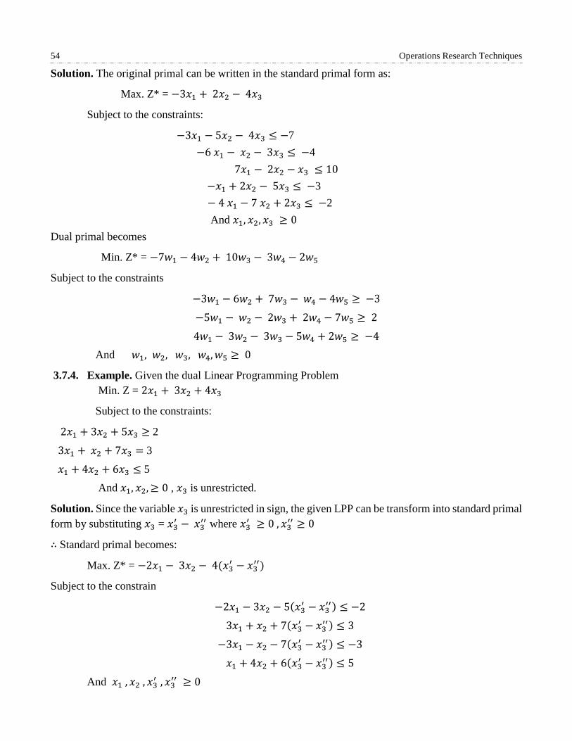
54 Operations Research Techniques
Solution. The original primal can be written in the standard primal form as:
Max. Z* = −3𝑥1 + 2𝑥2 − 4𝑥3
Subject to the constraints:
−3𝑥1 − 5𝑥2 − 4𝑥3 ≤ −7
−6 𝑥1 − 𝑥2 − 3𝑥3 ≤ −4
7𝑥1 − 2𝑥2 − 𝑥3 ≤ 10
−𝑥1 + 2𝑥2 − 5𝑥3 ≤ −3
− 4 𝑥1 − 7 𝑥2 + 2𝑥3 ≤ −2
And 𝑥1, 𝑥2, 𝑥3 ≥ 0
Dual primal becomes
Min. Z* = −7𝑤1 − 4𝑤2 + 10𝑤3 − 3𝑤4 − 2𝑤5
Subject to the constraints
−3𝑤1 − 6𝑤2 + 7𝑤3 − 𝑤4 − 4𝑤5 ≥ −3
−5𝑤1 − 𝑤2 − 2𝑤3 + 2𝑤4 − 7𝑤5 ≥ 2
4𝑤1 − 3𝑤2 − 3𝑤3 − 5𝑤4 + 2𝑤5 ≥ −4
And 𝑤1, 𝑤2, 𝑤3, 𝑤4, 𝑤5 ≥ 0
3.7.4. Example. Given the dual Linear Programming Problem
Min. Z = 2𝑥1 + 3𝑥2 + 4𝑥3
Subject to the constraints:
2𝑥1 + 3𝑥2 + 5𝑥3 ≥ 2
3𝑥1 + 𝑥2 + 7𝑥3 = 3
𝑥1 + 4𝑥2 + 6𝑥3 ≤ 5
And 𝑥1, 𝑥2, ≥ 0 , 𝑥3 is unrestricted.
Solution. Since the variable 𝑥3 is unrestricted in sign, the given LPP can be transform into standard primal
form by substituting 𝑥3 = 𝑥3′ − 𝑥3
′′ where 𝑥3′ ≥ 0 , 𝑥3
′′ ≥ 0
∴ Standard primal becomes:
Max. Z* = −2𝑥1 − 3𝑥2 − 4(𝑥3′ − 𝑥3
′′)
Subject to the constrain
−2𝑥1 − 3𝑥2 − 5(𝑥3′ − 𝑥3
′′) ≤ −2
3𝑥1 + 𝑥2 + 7(𝑥3′ − 𝑥3
′′) ≤ 3
−3𝑥1 − 𝑥2 − 7(𝑥3′ − 𝑥3
′′) ≤ −3
𝑥1 + 4𝑥2 + 6(𝑥3′ − 𝑥3
′′) ≤ 5
And 𝑥1 , 𝑥2 , 𝑥3′ , 𝑥3
′′ ≥ 0

Simplex Method and Duality in Linear Programming 55
∴ Required dual is
Min. Z* = −2𝑤1 + 3(𝑤2′ − 𝑥3
′′) + 5𝑤3
Subject to the constraints
−2𝑤1 + 5(𝑤2′ − 𝑥2
′′) + 𝑤3 ≥ −2
−3𝑤1 + (𝑤2′ − 𝑥2
′′) + 4𝑤3 ≥ −3
−5𝑤1 + 7(𝑤2′ − 𝑥2
′′) + 6𝑤3 ≥ −4
5𝑤1 − 7(𝑤2′ − 𝑥2
′′) − 6𝑤3 ≥ 4
And 𝑤1 , 𝑤2′ , 𝑤2
′′, 𝑤3 ≥ 0
Again, we write
Min. Z* = −2𝑤1 + 3𝑤2 + 5𝑤3
Subject to the constraints
−2𝑤1 + 5𝑤2 + 𝑤3 ≥ −2
−3𝑤1 + 𝑤2 + 4𝑤3 ≥ −3
5𝑤1 − 7𝑤2 − 6𝑤3 = 4 And 𝑤1 , 𝑤2 ≥ 0 and 𝑤3 is unrestricted.
3.7.5. Exercises.
1. Write the dual of the following Linear Programming Problem
Max. Z = 2𝑥1 + 3𝑥2 + 𝑥3
Subject to the constraints:
4𝑥1 + 3𝑥2 + 4𝑥3 = 6
𝑥1 − 2𝑥2 + 35 = 4
And 𝑥1, 𝑥2, 𝑥3 ≥ 0
Answer. Min. Z = 6(𝑤1 − 𝑤2) + 4(𝑤3 − 𝑤4)
Subject to the constraint
4(𝑤1 − 𝑤2) + (𝑤3 − 𝑤4) ≥ 2
3(𝑤1 − 𝑤2) + 2(𝑤3 − 𝑤4) ≥ 3
(𝑤1 − 𝑤2) + 5(𝑤3 − 𝑤4) ≥ 1
And 𝑤1, 𝑤2, 𝑤3 ≥ 0
2. Write the dual of the following Linear Programming Problem
Max. Z = 3𝑥1 − 2𝑥2
Subject to the constraints:
𝑥1 ≤ 4
𝑥2 ≤ 6
𝑥1 + 𝑥2 ≤ 5
−𝑥2 ≤ −1
And 𝑥1, 𝑥2, 𝑥3 ≥ 0

56 Operations Research Techniques
Answer. Min. Z*= 4𝑤1 + 6𝑤2 + 5𝑤3 − 1𝑤4
Subject to the constraints:
𝑤1 + 𝑤3 ≥ 3
𝑤2 + 𝑤3 − 𝑤4 ≥ −2 And 𝑤1, 𝑤2, 𝑤3,𝑤4 ≥ 0
3. Min. Z = 𝑥1 + 𝑥2 + 𝑥3
Subject to the constraints:
𝑥1 − 3𝑥2 + 4𝑥3 = 5
𝑥1 − 2𝑥2 ≤ 3
2𝑥1 − 𝑥3 ≥ 4
And 𝑥1, 𝑥2, ≥ 0 , 𝑥3 is unrestricted
Answer. Min. Z* = 5𝑤1 + 3𝑤2 − 4𝑤3
Subject to the constraints
𝑤1 + 𝑤2 − 2𝑤3 ≥ −1
−3𝑤1 − 2𝑤2 ≥ −1
4w1 + 0w2 − w3 ≥ −1
−4w1 + 0w2 + w3 ≥ 1 And 𝑤2 , 𝑤3 ≥ 0 and 𝑤3 is unrestricted.
4. Max. Z = 3𝑥1 + 𝑥2 + 𝑥3 − 𝑥4
Subject to the constraints:
𝑥1 − 5𝑥2 + 3𝑥3 + 4𝑥4 ≤ 5
𝑥1 + 𝑥2 = −1
𝑥3 − 𝑥4 ≥ −5
And 𝑥1, 𝑥2, 𝑥3, 𝑥4 ≥ 0
Answer. Min. Z* = 5𝑤1 − 𝑤2 + 5𝑤3
Subject to the constraints
𝑤1 + 𝑤2 ≥ 3
5𝑤1 + 𝑤2 ≥ 1
3𝑤1 − 𝑤3 ≥ 1
4𝑤1 + 𝑤3 ≥ −1
And 𝑤1 , 𝑤3 ≥ 0 and 𝑤2 is unrestricted.

Simplex Method and Duality in Linear Programming 57
3.8. CHECK FOR PROGRESS
1. Describe simplex method of solving linear programming problem.
2. Explain the term ‘Artificial variable’ and its use in linear programming.
3. What do you mean by two-phase method in linear programming problem?
4. Write a note on the use of Big-M method in solving linear programming problem.
5. Explain the concept of degeneracy in simplex method.
6. Explain the concept of duality.
7. Discuss relationship between primal and its dual.
3.9. SUMMARY
In this chapter, we study simplex method which can be used for solving LPP involving more than
two variables. Simplex method is an iterative method as it examines the extreme points in a
systematic manner, repeating the same set of steps until an optimal solution is reached. We have
introduced artificial variables which play an important role to solve an LPP involving greater-than-
or-equal to constraints and/or equality constraints.
Here, we discuss two important methods namely Big-M and Two-phase method for solving LPP
involving artificial variables. In this chapter, we introduce the concept of degeneracy which occurs
in a linear programming problem when in the simplex table one or more basic variable has value
zero or RR is not unique. In the last, we explain duality concept of LPPs which is very useful in
science and engineering, game theory, economics etc.

4 TRANSPORTATION PROBLEM
Structure
4.1. Introduction
4.2. Mathematical Formulation of the Transportation Problem
4.3. Methods of Finding Initial Basic Feasible Solution
4.4. Methods of Finding Optimal Solution
4.5. Unbalanced Transportation Problem
4.6. Degeneracy
4.7. Check Your Progress
4.8. Summary
4.1. INTRODUCTION
Transportation problem is a special kind of Linear Programming Problem (LPP) in which the objective is
to transport goods from a set of sources/origins to a set of destinations in such a manner that the total
transportation or shipping cost is minimized. To achieve this objective, we must know about some
parameters such as the quantity of available supplies, the quantity demanded and the costs of shipping a
unit from various origins to various destinations. Solving LPPs by simplex method discussed in chapter 3
involves a large number of variables and constraints and takes a long time to solve it. So, in this chapter,
we shall discuss the methods, which are specifically applied for solving transportation problems. Firstly,
we shall explain how to formulate mathematically a transportation problem and methods of finding initial
basic feasible solution. After finding the initial basic feasible solution, we discuss how optimality test is

Transportation Problem 59
performed by applying the Stepping Stone Method or Modified Distribution Method (MODI)to find
whether the obtained feasible solution is optimal or not. In the last, we shall explain the case of unbalanced
transportation problems and degeneracy.
4.1.1. Objectives
After studying this chapter, the reader should be able to:
Define a transportation problem.
Obtain the basic feasible solution of a transportation problem using North – West Corner Rule,
Least Cost and Vogel’s Approximation methods.
State the conditions for performing optimality test.
Explain the algorithm of the Stepping Stone and Modified Distribution (MODI) methods of
obtaining the optimal solution of a transportation problem.
Solve the transportation problems for special cases such as unbalanced transportation problem,
case of degeneracy.
4.2. MATHEMATICAL FORMULATION OF THE TRANSPORTATION PROBLEM
Let there be m origins/ sources of supply 𝑂1, 𝑂2, … , 𝑂𝑖 … 𝑂𝑚 and n destinations𝐷1, 𝐷2, … , 𝐷𝑗 … 𝐷𝑛 . The
total number of the capacities of all m origins is assumed to be equal to the total number of the
requirements of all n destinations. Let 𝐶𝑖𝑗 be the cost of shipping one unit from origin i to destination j.
Let 𝑎𝑖 be the capacity/ availability of items at origin i and 𝑏𝑗 , the requirement/demand of the destination
j. Then this transportation problem can be expressed in a tabular form as follows:
Origin Destinations
𝐷1 𝐷1 ... 𝐷𝑗 ... 𝐷𝑛
Availability/
capacity
𝑂1
𝑂2
𝑂𝑖
𝑂𝑚
𝐶11 𝐶12 ... 𝐶1𝑗 ... 𝐶1𝑛
𝐶21 𝐶22 ... 𝐶2𝑗 ... 𝐶2𝑗
. . . .
. . . .
. . . .
𝐶𝑖1 𝐶𝑖2 ... 𝐶𝑖𝑗 ... 𝐶𝑖𝑛
. . . .
. . . .
. . . .
𝐶𝑚1 𝐶𝑚2 ... 𝐶𝑚𝑗 ... 𝐶𝑚𝑛
𝑎1
𝑎2 .
.
.
𝑎𝑖 .
.
.
𝑎𝑚
Requirement/
Demand 𝑏1 𝑏2 ... 𝑏𝑗 ... 𝑏𝑛
Total
The condition for the existence of a feasible solution to a transportation problem is give as
∑ 𝑎𝑖 = ∑ 𝑏𝑗
𝑛
𝑗=1
𝑚
𝑖=1

60 Operations Research Techniques
The above equation tells us that the total requirement/demand equals the total capacity. If it is not so, a
dummy origin or destination is created to balance the total capacity and requirement.
Now let 𝑥𝑖𝑗 be the number of units to be transported from origin i to destination j and 𝐶𝑖𝑗 the corresponding
cost of transportation. Then the total transportation cost is ∑ .𝑚𝑖=1 ∑ 𝐶𝑖𝑗𝑥𝑖𝑗
𝑛𝑗=1
Subject to the constraints:
∑ 𝑥1𝑗 = 𝑎1 ,
𝑛
𝑗=1
∑ 𝑥2𝑗 = 𝑎2 ,
𝑛
𝑗=1
… , ∑ 𝑥𝑚𝑗 = 𝑎𝑚
𝑛
𝑗=1
……(3)
∑ 𝑥𝑖1 = 𝑏1 ,
𝑚
𝑖=1
∑ 𝑥𝑖2 = 𝑏2 ,
𝑚
𝑖=1
… , ∑ 𝑥𝑖𝑛 = 𝑏𝑛
𝑛
𝑗=1
And 𝑥𝑖𝑗 ≥ 0 for all i = 1, 2, 3... m and j = 1, 2... n.
The Simplex method is regarded as the most generalized method to solve this. However, the solution is
very lengthy and takes a long time to solve it since a large number of decision variables and artificial
variables are involved. It is far simpler to solve it by transportation method as compared to the Simplex
method. In the transportation method, we first obtain the initial basic feasible solution and then perform
the optimality test.
Note: A transportation problem is said to be balanced if it satisfies the condition ∑ 𝑎𝑖 = ∑ 𝑏𝑗𝑛𝑗=1
𝑚𝑖=1 .
4.3. METHODS OF FINDING INITIAL BASIC FEASIBLE SOUTION
There are several methods to obtain initial basic feasible solution. Here, we shall discuss the following
methods to determine the initial basic feasible solution:
(i) North-West Corner Rule
(ii) Least Cost Method
(iii) Vogel’s Approximation Method (Penalty or Regret Method)
Vogel’s Approximation method generally gives a solution closer to the optimum solution. Hence, it is
preferred to the other two methods.
4.3.1. North – West Corner Rule
The North – West Corner Rule (NWC)is a simple and efficient method to obtain initial basic feasible
solution. Itcan be summarized as follows:
Step 1: Start with cell (1, 1) at the north-west corner (upper left-hand corner) of the transportation
matrix and allocate as much as possible there.
Step 2: Here, we have three cases
(a) If the quantity needed at First Destination (𝑏1) is less than the quantity available at First Origin
(𝑎𝑖), we allocate a quantity equal to the requirement at First Destination to the cell (1, 1). At

Transportation Problem 61
this stage, Column 1 is exhausted, so we cross it out. Since the requirement 𝑏1 is fulfilled, we
reduce the availability 𝑎1 𝑏𝑦 𝑏1 and proceed to north-west corner of the resulting matrix, i.e.,
cell (1,2).
(b) If the quantity needed at First Destination (𝑏1) is greater than the quantity available at First
Origin(𝑎1), allocate a quantity equal to the quantity available at First Plant/Origin
(𝑎1 ) 𝑡𝑜 𝑐𝑒𝑙𝑙 (1, 1).At this stage, Row 1 is exhausted, so we cross it out and proceed to north-
west corner of the resulting matrix, i.e., cell (2, 1).
(c) If the quantity needed at First Destination (𝑏1) is equal to the quantity available at First Origin
(𝑎1), we allocate a quantity equal to the requirement at First Destination (or the quantity
available at First Origin). At this stage, both column 1 as well as Row 1 is exhausted. We cross
them out and proceed to the north-west corner of the resulting matrix, i.e., cell (2, 2).
Step 3: We continue the procedure, until we reach the south – east corner of the original matrix.
4.3.1.1. Example. Find the basic feasible solution of the given transportation problem by applying North
– West Corner rule:
Warehouse
Factory
D E F G Capacity
A
B
C
42 48 38 37
40 49 52 51
39 38 40 43
160
150
190
Requirement 80 90 110 220 500
Solution. We start from the North – West corner, i.e., the Factory A and Warehouse D. The quantity
needed at the First Warehouse (Warehouse D) is 80, which is less than the quantity available (160) at the
First Factory A. Therefore, a quantity equal to the warehouse D is to be allocated to the cell (A, D). Thus,
the requirement of Warehouse D is met by Factory A. So, we cross out column 1 and reduce the capacity
of Factory A by 80. Then we go to cell (A, E), which is North – West corner of the resulting matrix.
Now, the quantity needed at the second Warehouse (Warehouse E) is 90, which is greater than the quantity
available (80) at the First Factory A. Therefore, we allocate a quantity equal to the capacity at Factory A,
i.e., 80 to the cell (A, E). The requirement of Warehouse E is reduced to 10. The capacity of Factory A is
exhausted and has to be removed from the matrix. Therefore, we cross out row 1 and proceed to cell (B, E).
Now, the quantity needed at the second Warehouse (Warehouse E) is 10, which is less than the quantity
available at the Second Factory B, which is 150. Therefore, the quantity 10 equal to the requirement at
Warehouse E is allocated to the cell (B, E). Hence, the requirement of Warehouse E is met and we cross
out column 1. We reduce the capacity of Factory B by 10 and proceed to cell (B, F).

62 Operations Research Techniques
Again, the quantity needed at the Third Warehouse (Warehouse F) is 110. It is less than the quantity
available at the Second Factory (Factory B), which is140. Therefore, a quantity equal to the requirement
at Warehouse F is allocated to the cell (B, F). Since the requirement of Warehouse F is met, we cross out
Column 1 and reduce the capacity of Factory B by 110. Then we proceed to cell (B, G).Now, the quantity
needed at the Fourth Warehouse (Warehouse G) is 220, which is greater than the quantity available at the
Second Factory (Factory B).Therefore, we allocate the quantity equal to the capacity of Factory B to the
cell (B, G) so that the capacity of Factory B is exhausted and the requirement of Warehouse G is reduced
to 190. Hence, we cross out Row 1 and proceed to cell (C, G).
Thus, the allocations given using North – West corner rule are as shown in the following matrix along
with the cost per unit of transportation:
Warehouse
Factory
D E F G Capacity
A
B
C
42 48 38 37
40 49 52 51
39 38 40 43
160
150
190
Requirement 80 90 110 220 500
Thus, the total transportation cost for these allocations
= 42 × 80 + 48 × 80 + 49 × 10 + 52 × 110 + 51 × 30 + 43 × 190
= 3360 + 3840 + 490 + 5720 + 1530 + 8170 =23110
4.3.1.2. Exercise. Find the basic feasible solution of the following problem using North-West Corner
Rule:
Origin/
Distribution Centre
1 2 3 4 5 6 Availability
1
2
3
4
5
4 6 9 2 7 8
3 5 4 8 10 0
2 6 9 8 4 13
4 4 5 9 3 6
9 8 7 3 2 14
10
12
4
18
20
Requirements 8 8 16 3 8 21
Answer. Using North - West corner rule, the allocations are to be made as under:
8 units to cells (1,1), 2 units to cell (1,2), 6 units to cell (2,2), 6 units to cell (2,3), 4 units to cell (3 ,3), 6
units to cell (4,3), 3 units to cell (4,4), 8 units to cell (4,5), 1 unit to cell (4,6) and 20 units to cell (5,6)
and the transportation cost is equals to 501.
80 80
10 11
0
30
190
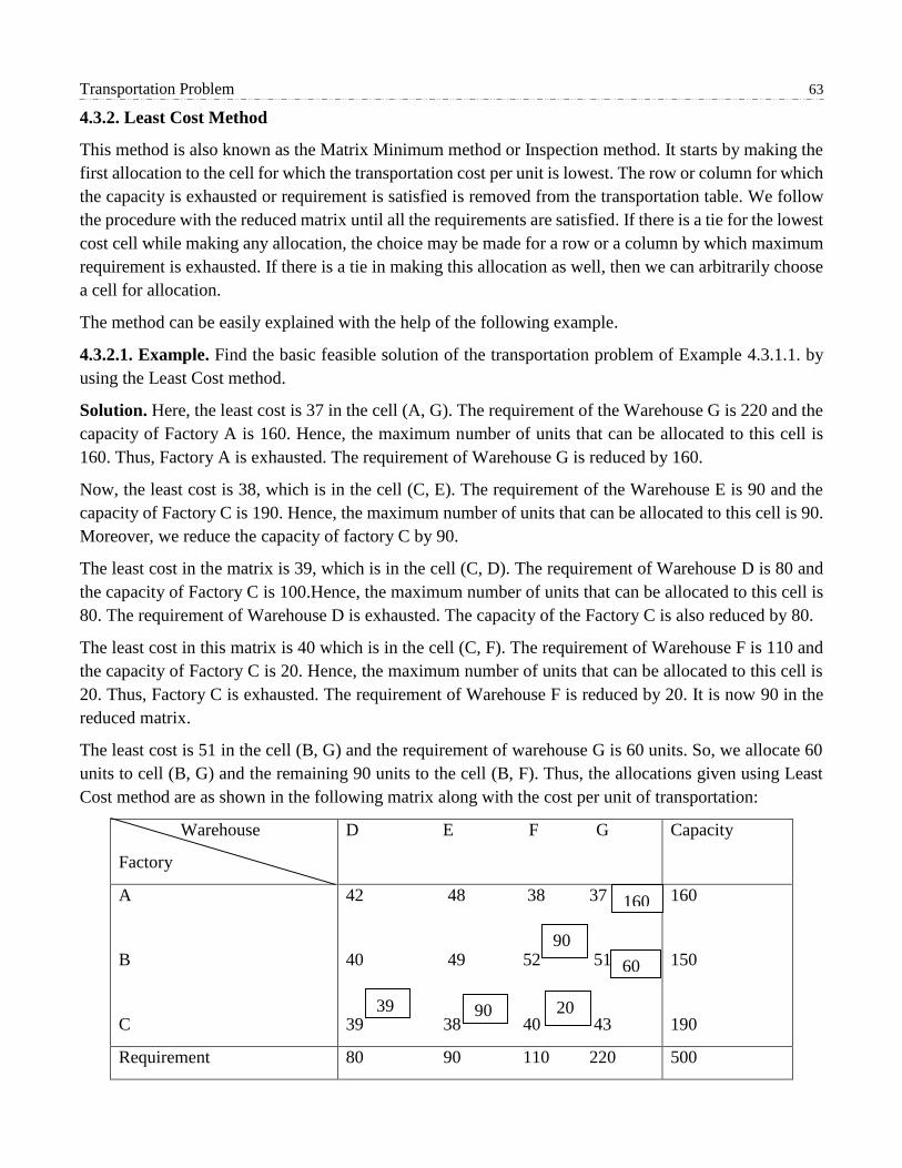
Transportation Problem 63
4.3.2. Least Cost Method
This method is also known as the Matrix Minimum method or Inspection method. It starts by making the
first allocation to the cell for which the transportation cost per unit is lowest. The row or column for which
the capacity is exhausted or requirement is satisfied is removed from the transportation table. We follow
the procedure with the reduced matrix until all the requirements are satisfied. If there is a tie for the lowest
cost cell while making any allocation, the choice may be made for a row or a column by which maximum
requirement is exhausted. If there is a tie in making this allocation as well, then we can arbitrarily choose
a cell for allocation.
The method can be easily explained with the help of the following example.
4.3.2.1. Example. Find the basic feasible solution of the transportation problem of Example 4.3.1.1. by
using the Least Cost method.
Solution. Here, the least cost is 37 in the cell (A, G). The requirement of the Warehouse G is 220 and the
capacity of Factory A is 160. Hence, the maximum number of units that can be allocated to this cell is
160. Thus, Factory A is exhausted. The requirement of Warehouse G is reduced by 160.
Now, the least cost is 38, which is in the cell (C, E). The requirement of the Warehouse E is 90 and the
capacity of Factory C is 190. Hence, the maximum number of units that can be allocated to this cell is 90.
Moreover, we reduce the capacity of factory C by 90.
The least cost in the matrix is 39, which is in the cell (C, D). The requirement of Warehouse D is 80 and
the capacity of Factory C is 100.Hence, the maximum number of units that can be allocated to this cell is
80. The requirement of Warehouse D is exhausted. The capacity of the Factory C is also reduced by 80.
The least cost in this matrix is 40 which is in the cell (C, F). The requirement of Warehouse F is 110 and
the capacity of Factory C is 20. Hence, the maximum number of units that can be allocated to this cell is
20. Thus, Factory C is exhausted. The requirement of Warehouse F is reduced by 20. It is now 90 in the
reduced matrix.
The least cost is 51 in the cell (B, G) and the requirement of warehouse G is 60 units. So, we allocate 60
units to cell (B, G) and the remaining 90 units to the cell (B, F). Thus, the allocations given using Least
Cost method are as shown in the following matrix along with the cost per unit of transportation:
Warehouse
Factory
D E F G Capacity
A
B
C
42 48 38 37
40 49 52 51
39 38 40 43
160
150
190
Requirement 80 90 110 220 500
39 90 20
90
160
60

64 Operations Research Techniques
Thus, the total transportation cost = 37× 160 + 52 × 90 + 51 × 80 + 38 × 90 + 40 × 20
= 21000
Note: This method has reduced the total transportation cost in comparison to the NWC rule.
4.3.2.2. Exercise. Find the basic feasible solution of the following problem using the Least Cost method:
Origin/
Distribution Centre
1 2 3 4 5 6 Availability
1
2
3
4
5
4 6 9 2 7 8
3 5 4 8 10 0
2 6 9 8 4 13
4 4 5 9 3 6
9 8 7 3 2 14
10
12
4
18
20
Requirements 8 8 16 3 8 21
Answer. Using Least Cost method, the allocations are to be made as under:
4 units to cell (1,1), 3 units to cell (1,4), 3 units to cell (1,6), 12 units to cell (2,6), 4 units to cell (3,1), 8
units to cell (4,2), 10 units to cell (4,3), 6 units to cell (5,3), 8 units to cell (5,5) and 6 units to cell (5,6).
The transportation cost = 278.
4.3.3. Vogel’s Approximation Method (VAM)
We describe the step by step procedure for finding the initial basic feasible solution by Vogel’s
Approximation method (Penalty method) in the following steps:
(i) In the transportation table calculate penalties for each row (column), by taking the difference
between the least and second least costs in the same row (column). We display it to the right
(below) of that row (column) in a new column (row) formed by extending the table on the right
(bottom). The new column and row formed by extending the table at the right and bottom are
labelled as penalty column and penalty row, respectively. The differences noted in the penalty row
or penalty column indicates the penalty or extra cost. If two cells in a row (or column) contain the
same least costs then the difference is taken as zero.
(ii) Select the row or column with the largest penalty (largest difference) and allocate the maximum
possible units to the least cost cell in the selected column or row. If there is a tie in the values of
penalties, the choice may be made for that row or column, which has the least cost. In case there
is a tie in such least cost as well, choice may be made from that there is a tie in such least cost as
well, choice may be made from that row or column by which maximum requirements are exhausted
.The cell so chosen is allocated the units and the corresponding exhausted row or column is
removed or ignored from further consideration.
(iii) Now, we determine the column and row differences for the reduced transportation table and repeat
the procedure until all column and row totals are exhausted.
This method is also known as the penalty method. Let us understand the procedure with the help
of an example.
4.3.3.1. Example. Apply the Vogel’s Approximation Method for finding the Basic Feasible Solution for
the transportation problem of Example 4.3.1.1.

Transportation Problem 65
Solution. In the first row, the least and the second least costs are 37 and 38 and their difference is 1. We
write 1 in a new column created on the right. It is labelled Penalty.Similarly, the differences between the
least and the second least costs in the second and third row, respectively, are 49 – 40 = 9 and 39 – 38 = 1.
So, we write the values (differences), i.e., 9 and 1 in the penalty column.
Next, we find the differences of the least and second least elements of each of the columns D, E, F and G.
These are 40-39 = 1, 48-38 = 10, 40-38 = 2 and 43-37 = 6, respectively. We write them in a newly created
penalty row at the bottom of the table.
We now select the largest of these differences in the penalty row and column, which are 10 in this case.
This value (10) corresponds to the second column (Column E) and the least cost in the column is 38.
Hence the allocation of 90 units (the maximum requirement of warehouse E) is to be made in the cell (C,
E) from Factory C. Since the column corresponding to E is exhausted, it is removed for the next reduced
matrix and the capacity of C is reduced by 90.
We now take the differences between the least and the Second least cost for each row and column of the
reduced matrix. In the first row, the least and the second least costs are 37 and 38 and their differences is
1. We write it in the newly created penalty column. Similarly, we write the second difference element 51-
40 = 11 and third difference element 40-39 = 1 in the second and third row of this column. Likewise, the
differences of the smallest and second smallest elements of each of the columns D, F, and G are 40–39 =
1, 4–38 = 2 and 43–37 = 6, respectively. We write these in a newly created penalty row at the bottom of
the table.
Now, we select the largest of these differences in the penalty row and column, which is 11 in this case.
This value (11) corresponds to Row B. Since the least cost in row is 40, we allocate 80 units (the maximum
requirement of Warehouse D) to the cell (B, D). Thus, the requirement of Warehouse D is exhausted and
we can remove it. We also reduce the capacity of Factory B by 80 in the next reduced matrix.
Again, in the first row, the least and the second least costs are 37 and 38 and their difference is 1. We write
it to the right of this row in the newly created penalty column. Similarly, the second and third elements in
the second and third rows of this column are 52–51=1 and
43–40 = 3, respectively. We write these in a newly created penalty row at the bottom of the table. Now,
we select the largest of these differences, which are 6 in this case. It corresponds to Column G and the
least cost in this column is 37. Hence, we allocate 160 units (the maximum capacity of Factory A) to the
cell (A, G). Since Row A is exhausted, it is removed for the next reduced matrix. We also reduce the
requirement of Warehouse G by 160 units.
Once again, the difference of the least costs in the first row is 52 – 51 = 1. We write it in the newly created
penalty column. Similarly, for the second row, the difference is 43-40 = 3. Likewise, the differences of
the least and second least elements of each of the columns F and G are 52 – 40 = 12 and 51 – 43 = 8,
respectively. We write them in the newly created penalty row at the bottom of the table. The largest of
these differences is 12 in this case. It corresponds to Column F and the least cost in this column is 40.
Hence, we allocate 100 units from the row (the maximum capacity of Factory C) to the cell (C, F). Since
Row C is exhausted, it is removed and the requirement of Warehouse F is reduced to 10 for the next
reduced matrix.

66 Operations Research Techniques
At the end, of the 70 units available in Factory B, we allocate 60 units to the lower cost (51), i.e., to the
cell (B, G) and the remaining 10 units to the cell (B, F).
The entire procedure of allocating units by Vogel’s Approximation Method is given in the following table:
Warehouse
Factory
D E F G Capacity Diff1 Diff2 Diff3 Diff4
A
B
C
Requirement
42 48 38 37 160
40 80 49 52 1051 60
39 38 90 40 100 43
80 90 110 220
160
150
190
500
1
9
1
1
11*
1
1
1
3
-
1
3
Diff1
Diff2
Diff3
Diff4
1 10* 2 6
1 - 2 6
- - 2 6*
- - 12* 8
Thus, the total transportation cost
=40 × 80 + 38 × 90 + 52 × 10 + 40 × 100 + 37 × 160 + 51 × 60
= 3200 + 3420 + 520 + 4000 + 5920 + 306 = 20120
Note: The total transportation cost obtained above is the lowest total transportation cost among the three
methods. Clearly the solution obtained by VAM is nearest to the optimal solution.
4.3.3.2. Exercise. Find the basic feasible solution of the following problem using Vogel’s Approximation
method:
Origin /Distribution
Centre
1 2 3 4 5 6
Availability
1
2
3
4
5
4 6 9 2 7 8
3 5 4 8 10 0
2 6 9 8 4 13
4 4 5 9 3 6
9 8 7 3 2 14
10
12
4
18
20
Requirement 8 8 16 3 8 21
Answer. The total transportation cost= 242.

Transportation Problem 67
4.4. METHODS OF FINDING OPTIMAL SOLUTION
Once an initial basic feasible solution is determined, the next step is to check its optimality. For this, we
performed an optimality test which tell us that whether the obtained feasible solution is optimal or not.
This can be done by applying one of the following methods:
(a) Stepping Stone Method
(b) Modified Distribution (MODI) Methods
These methods not only tell us about optimality of the initial basic feasible solution, they also
improve the solution until the optimal solution is obtained. Use of the Stepping Stone method is
convenient to a problem of small dimension as its application to a problem of a large dimension is
quite tedious and cumbersome.
The MODI method is usually preferred over the Stepping Stone method. Before studying the
methods of performing optimality test and finding optimal solutions, we introduce the concept of
independent allocations and state the conditions for performing optimality test.
4.4.1. Independent and Non-Independent Allocations
A set of allocations is said to be independent if they do not form a loop in the transportation table.
Here, formation of closed loop means that it is possible to travel from any allocation, back to itself
by a series of horizontal and vertical jumps from one occupied cell (i.e., the cell containing
allocation) to another, without a direct reversal of route (see Fig.). If such a loop can be formed
using some or all of the allocations under consideration, the allocations are known as non-
independent.
(a) (b)
Clearly allocations in (a) are independent allocations and of (b) are dependent.
Note: Every loop has an even number of cells.
4.4.2. Test for Optimality
An optimality test can be applied to the feasible solution only if it satisfies the following conditions:
(i) It contains exactly m+n-1 allocations where m and n represent the number of rows and
columns, respectively, of the transportation table.
(ii) These allocations are independent.
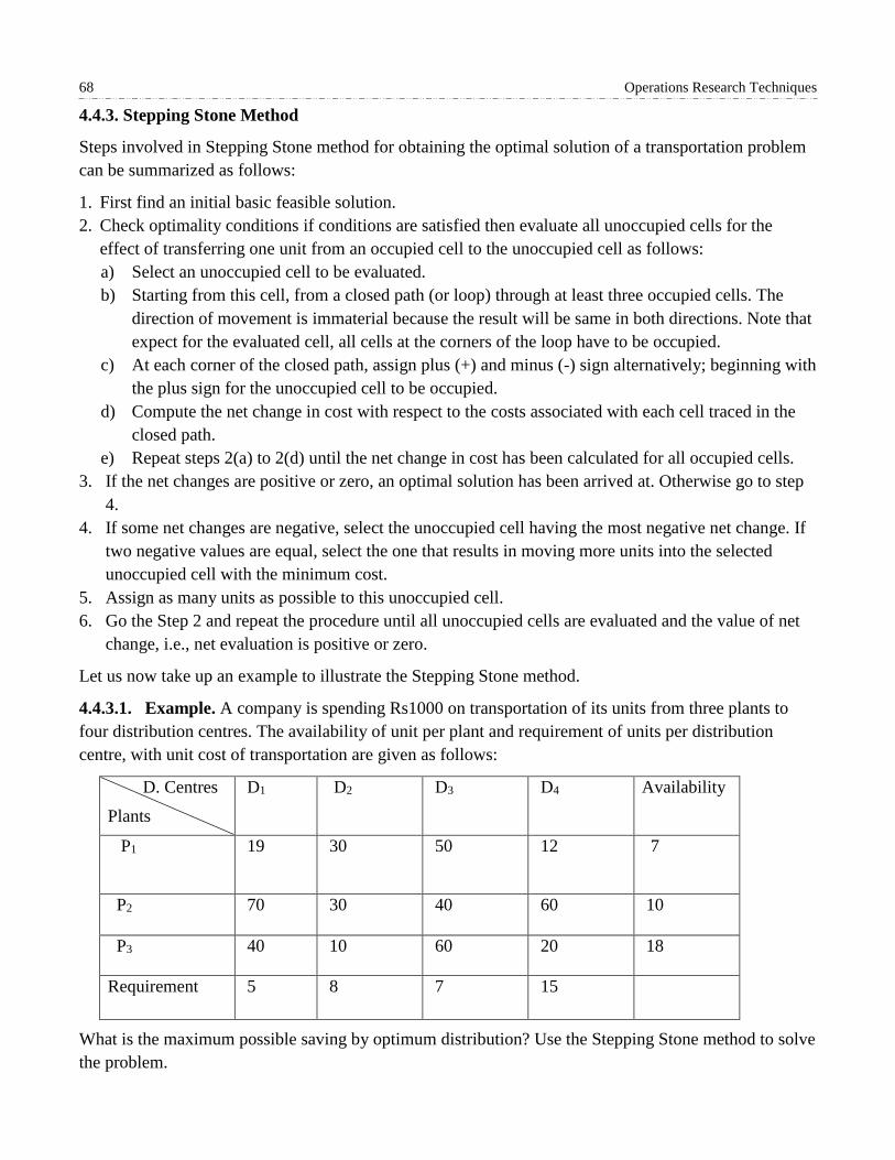
68 Operations Research Techniques
4.4.3. Stepping Stone Method
Steps involved in Stepping Stone method for obtaining the optimal solution of a transportation problem
can be summarized as follows:
1. First find an initial basic feasible solution.
2. Check optimality conditions if conditions are satisfied then evaluate all unoccupied cells for the
effect of transferring one unit from an occupied cell to the unoccupied cell as follows:
a) Select an unoccupied cell to be evaluated.
b) Starting from this cell, from a closed path (or loop) through at least three occupied cells. The
direction of movement is immaterial because the result will be same in both directions. Note that
expect for the evaluated cell, all cells at the corners of the loop have to be occupied.
c) At each corner of the closed path, assign plus (+) and minus (-) sign alternatively; beginning with
the plus sign for the unoccupied cell to be occupied.
d) Compute the net change in cost with respect to the costs associated with each cell traced in the
closed path.
e) Repeat steps 2(a) to 2(d) until the net change in cost has been calculated for all occupied cells.
3. If the net changes are positive or zero, an optimal solution has been arrived at. Otherwise go to step
4.
4. If some net changes are negative, select the unoccupied cell having the most negative net change. If
two negative values are equal, select the one that results in moving more units into the selected
unoccupied cell with the minimum cost.
5. Assign as many units as possible to this unoccupied cell.
6. Go the Step 2 and repeat the procedure until all unoccupied cells are evaluated and the value of net
change, i.e., net evaluation is positive or zero.
Let us now take up an example to illustrate the Stepping Stone method.
4.4.3.1. Example. A company is spending Rs1000 on transportation of its units from three plants to
four distribution centres. The availability of unit per plant and requirement of units per distribution
centre, with unit cost of transportation are given as follows:
D. Centres
Plants
D1 D2 D3 D4 Availability
P1 19
30 50 12 7
P2 70 30 40 60 10
P3 40 10 60 20 18
Requirement 5 8 7 15
What is the maximum possible saving by optimum distribution? Use the Stepping Stone method to solve
the problem.

Transportation Problem 69
Solution. First, we determine the initial feasible solution by applying VAM is given as follows:
D. Centers
Plant
D1 D2 D3 D4 Av. Diff1 Diff2 Diff3 Diff4
P1
P2
P3
19 5 30 50 122
70 30 40 7 60 3
40 10 8 6 20 10
7
10
18
7
10
10
18
10
10
38
20
40*
38
20
-
Requirement 5* 8 7 15
Diff1
Diff2
21* 20 10 8
- 20* 10 8
Diff3 - - 10 8
Diff4 - - 10 48*
In the above table, the encircled values are the allocations. The total transportation cost associated with
this initial basic feasible solution is
= 19 × 5 + 12 × 2 + 40 × 7 + 60 × 3 + 10 × 8 + 20 × 10
= 95 + 24 + 280 + 180 + 80 + 200 = 859
Clearly, here we have 3+4-1= 6 occupied cells. These are independent
as it is not possible to form any closed loop through these allocations
(see Fig.).
Hence, all the conditions of applying optimality test is satisfied so we
apply Stepping Stone method to obtain optimal solution.
Optimality Test using the Stepping Stone Method
We evaluate the effect of allocating one unit to each of the unoccupied cells making closed paths. Note
that the unoccupied cells are (P1,D2), (P1,D3),(P2,D1), (P2,D2), (P3,D1) and (P3,D3). We have to make closed
paths so that each path contains at least three occupied cells. We also have to evaluate the net change in
cost for each and every unoccupied cell. Then we have to select the one unoccupied cell, which has most
negative opportunity cost and allocate as many units as possible to reduce the total transportation cost.
The computations are shown as follows:
Unoccupied Cell Closed Path Net Change in Cost (Rs)
(P1, D2) (𝑃1, 𝐷2) → (𝑃1, 𝐷4) → (𝑃3, 𝐷4) → (𝑃3, 𝐷2) 30-12+20-10 = 28
(P1, D3) (𝑃1, 𝐷3) → (𝑃1, 𝐷4) → (𝑃2, 𝐷4) → (𝑃2, 𝐷3) 50-12+60-40 = 58
(𝑃2, 𝐷1) (𝑃2, 𝐷1) → (𝑃1, 𝐷1) → (𝑃1, 𝐷4) → (𝑃2, 𝐷4) 70-19+12-60 = 3
(𝑃2, 𝐷2) (𝑃2, 𝐷2) → (𝑃3, 𝐷2) → (𝑃3, 𝐷4) → (𝑃2, 𝐷4) 30-10+20-60 = -20
(𝑃3, 𝐷1) (𝑃3, 𝐷1) → (𝑃1, 𝐷1) → (𝑃1, 𝐷4) → (𝑃3, 𝐷4) 40-19+12-20 = 13
(𝑃3, 𝐷3) (𝑃3, 𝐷3) → (𝑃2, 𝐷3) → (𝑃2, 𝐷4) → (𝑃3, 𝐷4) 60-40+60-20 = 60

70 Operations Research Techniques
The cell (𝑃2, 𝐷2) has the most negative opportunity cost (net change in cost). Therefore, transportation
cost can be reduced by making allocation to this unoccupied cell. This means that if one unit is shifted to
this unoccupied cell through the loop shown in the fourth row of the table, then Rs20 can be saved (see
Fig.4.3a). hence, we shall shift as many units as possible to the cell (𝑃2, 𝐷2)through this loop. The
maximum number of units that can be allocated to (𝑃2, 𝐷2) through this loop is 3.
(𝑃2, 𝐷2) (𝑃2, 𝐷4)
(𝑃3, 𝐷2) (𝑃3, 𝐷4)
(a)
(b)
This is because the shifting can be done only from the corners of the loop and more than 3 units cannot
be shifted to (𝑃2, 𝐷2)as explained below:
The allocations at the corners of the loops are 3,10 and 8. If we try to shift more than 3 units, say, 4 units
from the corner (𝑃2, 𝐷4), then 4 units will have to be subtracted from the corner (𝑃3, 𝐷2) so that the total
of the column D4 remains unchanged. But this will give 3-4 = -1 allocations to the cell (𝑃2, 𝐷4), which is
impossible as negative allocations cannot be made.
We obtain the maximum number of units that can be allocated to the cell (𝑃2, 𝐷2) through the loop as
follows:
1. First, we assign (+) sign to the unoccupied cell (𝑃2, 𝐷2) to be evaluated and then (-) and (+) signs
alternatively to other corners of the closed loop (moving in one direction) as shown in Fig.4.3b.
2. Then we take the minimum of the values at the corners that have been assigned the negative sign.
In this case, the maximum number of units that can be allocated to the cell (𝑃2, 𝐷2) through the
mentioned loop is the minimum of 3 and 8. It is 3. So, we write it as:
min.{𝑡ℎ𝑒 𝑛𝑜. 𝑜𝑓 𝑢𝑛𝑖𝑡𝑠 𝑖𝑛(𝑃2, 𝐷4) = 3𝑡ℎ𝑒 𝑛𝑜. 𝑜𝑓 𝑢𝑛𝑖𝑡𝑠 𝑖𝑛 (𝑃2, 𝐷2) = 8
=3
The new table with these changes becomes:

Transportation Problem 71
D1 D2 D3 D4
P1
P2
P3
19 5 30 50 2 12
70 30 3 40 7 60
40 10 5 60 13 20
In the above table, note that we have also allocated 3 units from (P3, D2) to (P3, D4) so that column D4
remains unchanged. This leaves 5 units in the cell (P3, D2) and there are13 units in (P3, D4). The total
transportation cost associated with this solution is
Total cost =19 × 5 + 12 × 2 + 30 × 3 + 40 × 7 + 10 × 5 + 20 × 13
= 95 + 24 + 90 + 280 + 50 + 260 = 799
Now, we repeat the optimality test to see if further allocation can be made to reduce the total
transportation cost. The computation for the unoccupied cells is as follows:
Unoccupied
Cell
Closed Path Net Change in Cost (Rs)
(P1, D2) (𝑃1, 𝐷2) → (𝑃1, 𝐷4) → (𝑃3, 𝐷4) → (𝑃3, 𝐷2) 30-12+20-10 = 28
(P1, D3) (𝑃1, 𝐷3) → (𝑃1, 𝐷4) → (𝑃3, 𝐷4) → (𝑃3, 𝐷2)
→ (𝑃2, 𝐷2) → (𝑃2, 𝐷3)
50-12+20-10+30-40 = 38
(𝑃2, 𝐷1) (𝑃2, 𝐷1) → (𝑃1, 𝐷1) → (𝑃1, 𝐷4) → (𝑃3, 𝐷4)
→ (𝑃3, 𝐷2) → (𝑃2, 𝐷2)
70-19+12-20+10-30 = 23
(𝑃2, 𝐷2) (𝑃2, 𝐷4) → (𝑃3, 𝐷4) → (𝑃3, 𝐷2) → (𝑃2, 𝐷2) 60-20+10-30 = 20
(𝑃3, 𝐷1) (𝑃3, 𝐷1) → (𝑃1, 𝐷1) → (𝑃1, 𝐷4) → (𝑃3, 𝐷4) 40-19+12-20 = 13
(𝑃3, 𝐷3) (𝑃3, 𝐷3) → (𝑃2, 𝐷3) → (𝑃2, 𝐷2) → (𝑃3, 𝐷2) 60-40+30-10 = 40
Since, all opportunity costs in the unoccupied cells are non-negative, the current solution is an optimal
solution with total transportations cost 799. Hence the maximum saving by optimum distribution is
(1000-799) = 201.
Note: The Stepping Stone method should be applied only to problems of small dimensions as it becomes
quite tedious for large dimensions. To solve large dimensions problems, we use another method known
as (MODI). This method may be conveniently applied to problems of small dimension as well.
4.4.4. Modified Distribution Method (MODI)
The difference between the two methods is that in the Stepping Stone method, closed loops are drawn for
all unoccupied cells for determining their opportunity costs. However, in the MODI method, the
opportunity costs of all the unoccupied cells are calculated and the cell with opportunity costs of all the
unoccupied cells are calculated and the cell with the highest negative opportunity cost is identified without
drawing any closed loop. Then only one loop is drawn for the highest negative opportunity cost. The

72 Operations Research Techniques
procedure for finding out the optimal solution of a transportation problem with the help of the MODI
method is summarized in the following steps:
(i) First find an initial feasible solution using a suitable method.
(ii) Check optimality conditions for the current basic feasible solution if it has exactly (m+n-1)
independent allocations, write the cost matrix for only the allocated cells.
(iii) Now, by using this cost matrix, determine the set of m+n numbers 𝑢𝑖(i =1,2,…,m) and
𝑣𝑗 (j=1,2,..,n) such that for each occupied cell (i, j), 𝐶𝑖𝑗 = 𝑢𝑖 + 𝑣𝑗 , taking one of 𝑢𝑖 or 𝑣𝑗 as zero.
(iv) Fill the vacant cells using 𝑢𝑖 + 𝑣𝑗 .
(v) Compute all net evaluations (unit cost differences) ∆𝑖𝑗= 𝐶𝑖𝑗 − (𝑢𝑖 + 𝑣𝑗) by subtracting the values
so obtained in Step 4 from the corresponding values of the original cost matrix.
(vi) Examine the sign of each ∆𝑖𝑗
(a) If all ∆𝑖𝑗> 0, for all i, j; then the current basic feasible solution is an optimal solution.
(b) If all ∆𝑖𝑗≥ 0, for all i, j and at least one ∆𝑖𝑗 is zero then the current basic feasible solution is an
optimal solution and alternate optimal solution exists.
(c) If some of ∆𝑖𝑗< 0 for some (i, j), the current solution is not optimal. Then select the cell having
the most negative ∆𝑖𝑗 and tick it.
(vii) Construct a closed path/loop for the unoccupied cell ticked in Step 5(ii) using the already
allocated cells. At each corner of the closed path, assign plus (+) and minus (-) signs alternatively,
beginning with the plus sig for the unoccupied cell. Then 𝜃 units are to be allocated to this cell and
the same numbers of units are to be added and subtracted alternatively at the corners assigned plus
and minus signs, respectively.
The value of 𝜃 is the maximum number of units that can be allocated to this cell through the loop. It is
obtained by equating the allocations at the negative sign corners to zero. In this way, allocations have
been improved.
(viii) Write the cost matrix for only those cells which have improved allocations. Go to Step 3 and repeat
the procedure until all ∆𝑖𝑗≥ 0. Calculate the associated total transportation cost.
4.4.4.1. Example. Apply the MODI method for the problem taken in example 4.4.2.1.
Solution. We find initial basic feasible solution of the problem by VAM as given in table and check
optimality conditions
D. Centres
Plant
D1 D2 D3 D4 Av.
P1
P2
P3
Requirement
19 5 30 50 12 2
70 30 40 7 60 3
40 10 8 60 20 10
5 8 7 15
7
10
18
35

Transportation Problem 73
Now we perform optimality test by applying the MODI method. First of all, we write the cost matrix
for only allocated cells:
19 12 𝑢1
40 60 𝑢2
10 20 𝑢3
𝑣1 𝑣2 𝑣3 𝑣4
Let us denote the row numbers by 𝑢1, 𝑢2, 𝑢3and column numbers by 𝑣1,𝑣2,𝑣3and 𝑣4such that
𝑢1 + 𝑣1 = 19, 𝑢1 + 𝑣4 = 12, 𝑢2 + 𝑣3 = 40,
𝑢2 + 𝑣4 = 60, 𝑢3 + 𝑣2 = 10, 𝑢3 + 𝑣4 = 20.
Taking 𝑢1=0, we have 𝑣1 = 19 and 𝑣4 = 12 from the first two equations.
Putting the value of 𝑣4 in the fourth equation, we have 𝑢2 = 48.
Similarly, we find 𝑢3 = 8, 𝑣2 = 2 𝑎𝑛𝑑 𝑣3 = −8
Using these values, we fill the vacant cells of the above table using 𝐶𝑖𝑗 = 𝑢𝑖 + 𝑣𝑗 and put dots in the
already filled cells so that these cells are not considered again.
𝑣1 = 19 𝑣2 = 2 𝑣3 = −8 𝑣4 = 12
𝑢1 = 0 2 -8
𝑢2 = 48 67 50
𝑢3 = 8 27 0
Now, subtracting these values from the corresponding values of the original cost matrix, we have the
net evaluations, i.e., ∆𝑖𝑗= 𝐶𝑖𝑗 − (𝑢𝑖 + 𝑣𝑗)
30-2=28 50-(-8) =58
70-67=3 30-50= -20
40-27=13 60-0=60
Since Note that the cell (𝑃2, 𝐷2)has the most negative opportunity cost (net change in cost).
Therefore, the transportation cost can be reduced by making allocation to this unoccupied cell. This
means that if one unit is shifted to this unoccupied cell through the closed loop formed, beginning
from this cell and using allocated cells, Rs20 can be saved. We form the loop beginning from this
cell, i.e., the cell (𝑃2, 𝐷2) (see Fig. 4.4). We shift 𝜃 units to this unoccupied cell through the loop and
add and subtract 𝜃 from the cells at the other corners of the loop which are assigned ‘+’ and ‘-‘
signs. So, we get
𝜃 3- 𝜃
8− 𝜃 10+ 𝜃
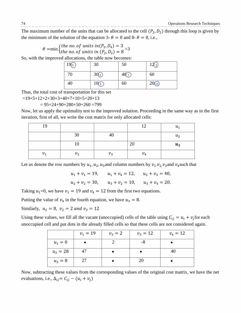
74 Operations Research Techniques
The maximum number of the units that can be allocated to the cell (𝑃2, 𝐷2) through this loop is given by
the minimum of the solution of the equation 3- 𝜃 = 0 and 8- 𝜃 = 0, i.e.,
𝜃 =min.{𝑡ℎ𝑒 𝑛𝑜. 𝑜𝑓 𝑢𝑛𝑖𝑡𝑠 𝑖𝑛(𝑃2, 𝐷4) = 3𝑡ℎ𝑒 𝑛𝑜. 𝑜𝑓 𝑢𝑛𝑖𝑡𝑠 𝑖𝑛 (𝑃2, 𝐷2) = 8
=3
So, with the improved allocations, the table now becomes:
19 5 30 50 12 2
70 30 3 40 7 60
40 10 5 60 20 13
Thus, the total cost of transportation for this set
=19×5+12×2+30×3+40×7+10×5+20×13
= 95+24+90+280+50+260 =799
Now, let us apply the optimality test to the improved solution. Proceeding in the same way as in the first
iteration, first of all, we write the cost matrix for only allocated cells:
19 12 𝑢1
30 40 𝑢2
10 20 𝒖𝟑
𝑣1 𝑣2 𝑣3 𝑣4
Let us denote the row numbers by 𝑢1, 𝑢2, 𝑢3and column numbers by 𝑣1,𝑣2,𝑣3and 𝑣4such that
𝑢1 + 𝑣1 = 19, 𝑢1 + 𝑣4 = 12, 𝑢2 + 𝑣3 = 40,
𝑢2 + 𝑣2 = 30, 𝑢3 + 𝑣2 = 10, 𝑢3 + 𝑣4 = 20.
Taking 𝑢1=0, we have 𝑣1 = 19 and 𝑣4 = 12 from the first two equations.
Putting the value of 𝑣4 in the fourth equation, we have 𝑢3 = 8.
Similarly, 𝑢2 = 8, 𝑣2 = 2 𝑎𝑛𝑑 𝑣3 = 12
Using these values, we fill all the vacant (unoccupied) cells of the table using 𝐶𝑖𝑗 = 𝑢𝑖 + 𝑣𝑗for each
unoccupied cell and put dots in the already filled cells so that these cells are not considered again.
𝑣1 = 19 𝑣2 = 2 𝑣3 = 12 𝑣4 = 12
𝑢1 = 0 2 -8
𝑢2 = 28 47 40
𝑢3 = 8 27 20
Now, subtracting these values from the corresponding values of the original cost matrix, we have the net
evaluations, i.e., ∆𝑖𝑗= 𝐶𝑖𝑗 − (𝑢𝑖 + 𝑣𝑗)

Transportation Problem 75
28 38
23 20
13 40
Since none of the net evaluation is negative, this solution is optimal. Thus, the total minimum
transportation cost is Rs799 and the maximum saving = (1000-799) = 201.
4.5. UNBALANCED TRANSPORTATION PROBLEM
The transportation problem wherein the total capacity of all sources and total requirement (demand) of all
destinations are not equal is called the unbalanced transportation problem. An unbalanced transportation
problem may occur in two different forms (i) Excess of availabilities (ii) Shortage in availabilities. In case
(i), we add a dummy destination in the transportation table with zero transportation cost. The requirement
of this dummy destination is assumed to be equal to the difference of total availability of sources and total
demand so that the problem becomes balanced. Similarly, in case (ii) we introduce a dummy source and
take the corresponding steps. The following example explain the whole procedure.
4.5.1. Example. A company has factories at A, B and C which supply warehouses at D, E, F, and G. The
monthly factory capacities are 160, 150 and 190 units, respectively. Monthly warehouse requirements are
80, 90, 110 and 160, respectively. Unit shopping costs (in rupees) are as follows:
From
To
D E F G
A 42 48 38 37
B 40 49 52 51
C 39 38 40 43
Determine the optimum distribution for this company to minimize shipping costs.
Solution. Here the total capacity of sources (factories) is 160 + 150 + 190 = 500. It is greater than the
total requirement of all the destinations (warehouses) which is 80 + 90 + 110 + 160 = 440.
Therefore, we added dummy destination in the transportation table with zero transportation cost and take
60 as its requirement. Thus, the problem becomes balanced that is the total capacity and total
requirement are equal the balanced., the problem is as follows:
From
To Capacity
D E F G H
A 42 48 38 37 0 160
B 40 49 52 51 0 150
C 39 38 40 43 0 190
Requirement 80 90 110 160 60 500
We can solve this problem using VAM to determine the basic feasible solution and then use MODI
method to find the optimal solution. We have solved this problem in Example 3. You may like to try the
remaining solution yourself.

76 Operations Research Techniques
The optimum allocation is:
160 to (A, F), 80 to (B, D), 10 to (B, E), 60 to (B, G), 80 to (C, E) and 110 to (C, F).
Note: If the number of allocations in the basic feasible solution is less than m + n – 1, we first go
through the special case of degeneracy and then apply the test of optimality.
4.6. DEGENRACY
Degeneracy occurs in the transportation problem if the number of occupied cells is less than m + n – 1.
To resolve degeneracy, we introduce an infinitesimally allocation e (say)in the least cost and
independent cell so that number of occupied cells becomes m+n-1. Also notice that if ‘e’ is added to or
subtracted from any quantity, the quantity remains unaltered.
Remark: We do not write 0 in place of e as it is one of the allocations and will not come into counting if
it is written as 0 so we write e and not 0 in its place and count it as one of the allocations.
Degeneracy occurs in Example 4.5.1. To solve this problem, we proceed as follows:
Using Vogel Approximation method, we get the basic feasible solution as:
Warehouse
Factory
D E F G H
Av.
D1 D2 D3 D4
A
B
C
42 48 38 37 160 0 e
40 80 49 52 10 51 60 0 60
39 38 90 40 100 43 0
160
150
190
37
40*
38
1
9
1
1
11*
3
1
1
3
Requirement 80 90 110 160 60 500
Diff1
Diff2
Diff3
Diff4
1 10 2 6 0
1 10* 2 6 -
1 - 2 6 -
- - 2 6* -
Here the number of allocations is 6 but the number of allocations should be 3 + 5 – 1 = 7 to perform
optimality test. Hence it is the case of degeneracy to resolve such a problem, we introduce infinitesimally
small allocation e in the least cost and independent cell, i.e., the cell (A,H). Another cell (C, H) also has
same least cost as the cell (A, H). But this cell is not independent because a loop (C,H)→ (C,F) → (B,F) →
(B,H) can be formed beginning with the cell as shown in figure 4.5. Now the number of allocations is 7,
i.e., as many as required for performing the optimality test.
42 48 38 0
49 (B, F) 51 (B, H)
39 (C, F) 43 0 (C, H)

Transportation Problem 77
Thus, applying optimality test by MODI method, the improved allocations after first iteration will be:
42 48 38 e 37 160 0
40 80 49 52 10 51 0 60
39 38 90 40 100 43 0
Again, applying the optimality test, the improved solution is
D E F G H
A 42 48 38 e 37 160 0
B 40 80 49 10 52 51 0 60
C 39 38 80 40 110 43 0
Again, applying the optimality test, you will see that these allocations give the optimal solution and the
total transportation cost = rupees 17050.
4.7. CHECK YOUR PROGRESS
1. Explain transportation problem. Is this a linear programming problem?
2. Explain method for obtaining initial basic feasible solution of Transportation problem:
(i) The North-West Corner Rule,
(ii) Vogel’s Approximation Method (VAM),
(iii) The least Cost Method.
3. Describe the computational procedure of the following optimality tests for solving transportation
problem:
(i) Stepping stone method,
(ii) MODI method.
4. Write a short note on unbalanced transportation problem.
5. What is degeneracy in a transportation problem?
4.8. SUMMARY
In this chapter, we have introduced transportation problems. As one can express these problems in terms
of LPPs so transportation problems is also considered as one of the sub – classes of Linear Programming
Problems and the objective of the problem is to determine the optimal amount to ship/ transport from
each origin to destination. Here, we have explained how to formulate mathematically a transportation
problem, finding initial basic feasible solution, performing optimality test and moving towards optimal
solution.
In this chapter, we have discussed three methods for finding initial basic feasible solution namely
North – West Corner Rule, Least Cost Method and Vogel's Approximation Method. Vogel’s
approximations method is preferred over other methods of finding the initial basic feasible solutions as it
generally gives the solution closest to the optimum solution. After finding the initial basic feasible
solution, optimality test is performed by applying the Stepping Stone Method or Modified Distribution
Method (MODI)to find whether the obtained feasible solution is optimal or not. In the last we have
discussed the case of unbalanced transportation problems and degeneracy.

5 ASSIGNMENT PROBLEMS
Structure
5.1. Introduction
5.2. Assignment Problems
5.3. Hungarian Method
5.4. Unbalanced Assignment Problem
5.5. Case of Maximization of an Assignment Problem
5.6. Travelling Salesman Problem
5.7. Check Your Progress
5.8. Summary
5.1. INTRODUCTION
Assignment problem is a special type/case of transportation problem and hence is of linear
programming problem which deals with the allocation of the various resources to the various activities on
one to one basis. It does it in such a manner that the cost or time involved in the process is minimum and
profit or sale is maximum. In chapter 4, we have already discussed methods of finding optimal solution
for the given problem but here we discuss another method namely Hungarian method for solving an
assignment problem. Hungarian method is shorter and easier than stepping stone and MODI methods
which we have discussed in previous chapter. In this chapter, we shall explain the assignment problems
including travelling salesman problem and apply Hungarian method for solving these problems.

Assignment Problems 79
5.1.1. Objectives
After studying this chapter, reader should be able to explain the following concepts like:
Assignment Problems
Hungarian Method.
Unbalanced Assignment Problem
Case of Maximization of an Assignment Problem
Travelling Salesman Problem
5.2. ASSIGNMENT PROBLEMS
An assignment problem may be considered as a special type of transportation problem in which there are
as many jobs/sources as the number of machines/destinations so that the jobs can be assigned to machines
in a one-to-one way only. The capacity of each source as well as the requirement of each destination is
taken as 1. The main difference between an assignment problem and transportation problem is that in the
case of assignment problem, the given matrix must necessarily be a square matrix which is not the
condition for a transportation problem.
Let there be n persons and n jobs and let 𝐶𝑖𝑗 represents the amount of time taken by 𝑖𝑡ℎ person to complete
the 𝑗𝑡ℎ job then our objective is assignment of jobs on one-to-one basis in such a way that the total cost is
minimum. The assignment problem can be stated in the form of an n×n matrix of real numbers called the
cost matrix as given in the following table:
Person
Job
1 2 … j … n
1
2
.
.
.
i
.
.
.
n
𝐶11𝐶12 … 𝐶1𝑗 … 𝐶1𝑛
𝐶21𝐶22 … 𝐶2𝑗… 𝐶2𝑛
.
.
.
𝐶𝑖1𝐶𝑖2… 𝐶𝑖𝑗 … 𝐶𝑖𝑛
.
.
.
𝐶𝑛1𝐶𝑛2… 𝐶𝑛𝑗… 𝐶𝑛𝑛
Let 𝑥𝑖𝑗 denote the 𝑗𝑡ℎ job assigned to the 𝑖𝑡ℎ person. Then, mathematically, the assignment problem can
be stated as follows:
Minimize Z = ∑ ∑ 𝑐𝑖𝑗𝑥𝑖𝑗𝑛𝑗=1
𝑛𝑖=1 , where i= 1, 2, …, n and j=1, 2, …, n.
subject to
𝑥𝑖𝑗 = {1 𝑖𝑓 𝑡ℎ𝑒 𝑖𝑡ℎ person is assigned the 𝑗𝑡ℎ job
0 𝑖𝑓 𝑡ℎ𝑒 𝑖𝑡ℎ person is not assigned the 𝑗𝑡ℎ job

80 Operations Research Techniques
Since one job assigned to one person only, we have
𝑥𝑖1 + 𝑥𝑖2+ … + 𝑥𝑖𝑛 = 1, i= 1, 2, …, n
𝑥1𝑗 + 𝑥2𝑗+ … + 𝑥𝑛𝑗 = 1, j= 1, 2, …, n
Note: The constant 𝑐𝑖𝑗 in the above problem represents time, in many situations it may be cost or some
other parameter which is to be minimized in the assignment problem under consideration.
Remark: An assignment problem can be looked upon as a special type of transportation problem in which
the jobs stands for sources, the machines for destinations and all the availabilities and requirements are
equal to one.
5.3. HUNGARIAN METHOD
Hungarian method is also known as Reduced Matrix Method, it is an efficient method for solving
assignment problems. Hungarian method is developed by Hungarian mathematician D. Konig. The step
by step procedure for obtaining an optimal solution of an assignment problem are as follows:
1. Develop the cost table from the given problem then check whether the given matrix is square i.e.
is number of sources/machines is equal to the number of destinations/jobs. If not, make it square
by adding a suitable number of dummy row (or column) with 0 cost/time element.
2. Locate the smallest cost element in each row of the given cost matrix and then subtract the smallest
element of each column from every element of that column.
3. In the resulting cost matrix, locate the smallest element in each column and subtract the smallest
element of each column from every element of that column.
4. In the modified matrix, search for an optimal assignment as follows:
a) Examine the row successively until a row with exactly one zero is found. Draw a rectangle around
this zero like 0 and cross out all other zeroes in the corresponding column. Proceed in this way
until all the row have been considered. If there is more than one zero in any row, don’t touch that
row, pass on to the next row.
b) Repeat step (a) above for the columns of the resulting cost matrix.
c) If a row or column of the reduced matrix contains more than one zeroes, arbitrarily choose a row or
column having the minimum number of zeroes. Arbitrarily select any zero in the row or column so
chosen. Draw a rectangle around it and cross out all the zeroes in the corresponding row and column.
Repeat steps (a), (b), and (c) until all the zeroes have either been assigned (by drawing a rectangle
around them) or crossed.
d) If each row or column of the resulting matrix has one and only one assigned zero, i.e. number of
assigned zeroes are equal to the number of rows/columns, then the optimum assignment is made in the
cells corresponding to 0 and the optimum solution of the problem is attained and we can stop here.
Otherwise, go to the next step.
5. Draw the minimum number of horizontal and/or vertical lines through all the zeroes as follows:
i. Mark (√ ) the rows in which assignment has not been made.
ii. Mark (√ ) column, that have zeroes in the marked rows.

Assignment Problems 81
iii. Mark (√ ) rows( not already marked ) which have assignments in marked columns. Then
mark (√ ) columns, which have zeroes in newly marked rows, if any. Mark (√ ) rows (not
already marked ), which have assignments in these newly marked columns.
6. Revise the cost matrix as follows:
i. Find the smallest elements not covered by any of the lines.
ii. Subtract this from all the uncovered elements and add it to the elements at the
intersection of the two lines.
iii. Other elements covered by the lines remain unchanged.
7. Repeat the procedure until an optimal solution attained.
Note: By drawing lines through all the unmarked rows and marked columns, we will get the required
minimum number of lines.
The following example illustrate the method.
5.3.1. Example. A computer centre has four expert programmers & needs to develop four application
programmes. The head of the computer Centre, estimates the computer time (in minutes) required by the
respective experts to develop the application programmes as follows:
PROGRAMMES
PROGRAMMERS
A B C D
1 120 100 80 90
2 80 90 110 70
3 110 140 120 100
4 90 90 80 90
Find the assignment pattern that minimize the time required to develop the application programmes.
Solution. Let us subtract the minimum element of each row from every element of that row. Note that the
minimum element in the first row is 80. So, 80 is subtracted from every element of the first row. Similarly,
we obtain the elements of the other rows of the resulting matrix. Thus, the modified matrix is:
A B C D
1 40 20 0 10
2 10 20 40 0
3 10 40 20 0
4 10 10 0 10
Let us now subtract the minimum element of each column from every element of that column in the
resulting matrix. The minimum element in the first column is 10. So, 10 is to be subtracted from every
element of the first column. Similarly, we obtain the elements of the other columns of the resulting matrix.
Thus, the resulting matrix is:

82 Operations Research Techniques
A B C D
1 30 10 0 10
2 0 10 40 0
3 0 30 20 0
4 0 0 0 10
Now starting from the first row onward, we draw a rectangle around the zero in each row having a single
zero and cross all other zeros in the corresponding column. Here, in the very first row we find a single
zero. So, we draw a rectangle around it and cross all the other zeroes in the corresponding column. We get
A B C D
1 30 10 0
10
2 0 10 40 0
3 0 30 20 0
4 0 0 0 10
In the second, third and fourth row, there is no single zero. Hence, we move column – wise. In the second
column, we have a single zero. Hence, we draw a rectangle around it and cross all other zeroes in the
corresponding row. We get
A B C D
1 30 10 0
10
2 0 10 40 0
3 0 30 20 0
4 0 0
0 10
In the matrix above, there is no row or column, which has a single zero. Therefore, we first move row –
wise to locate the row having more than one zero. The second row has two zeroes. So, we draw a rectangle
arbitrarily around one of these zeroes and cross the other one. Let us draw a rectangle around the zero in
the cell (2, A) and cross the zero in cell (2, D). We cross out the other zeroes in the first column. Note
that we could just as well have selected zero in the cell (2, D), drawn a rectangle around it and crossed all
other zeroes. This would have led to an alternative solution.
In this way, we are left with only one zero in every row and column around which a rectangle has been
drawn. This means that we have assigned only one operation to one operator. Thus, we get the optimum
solution as follows:
A B C D
1 30 10 0
10
2 0
10 40 0
3 0 30 20 0
4 0 0
0 10
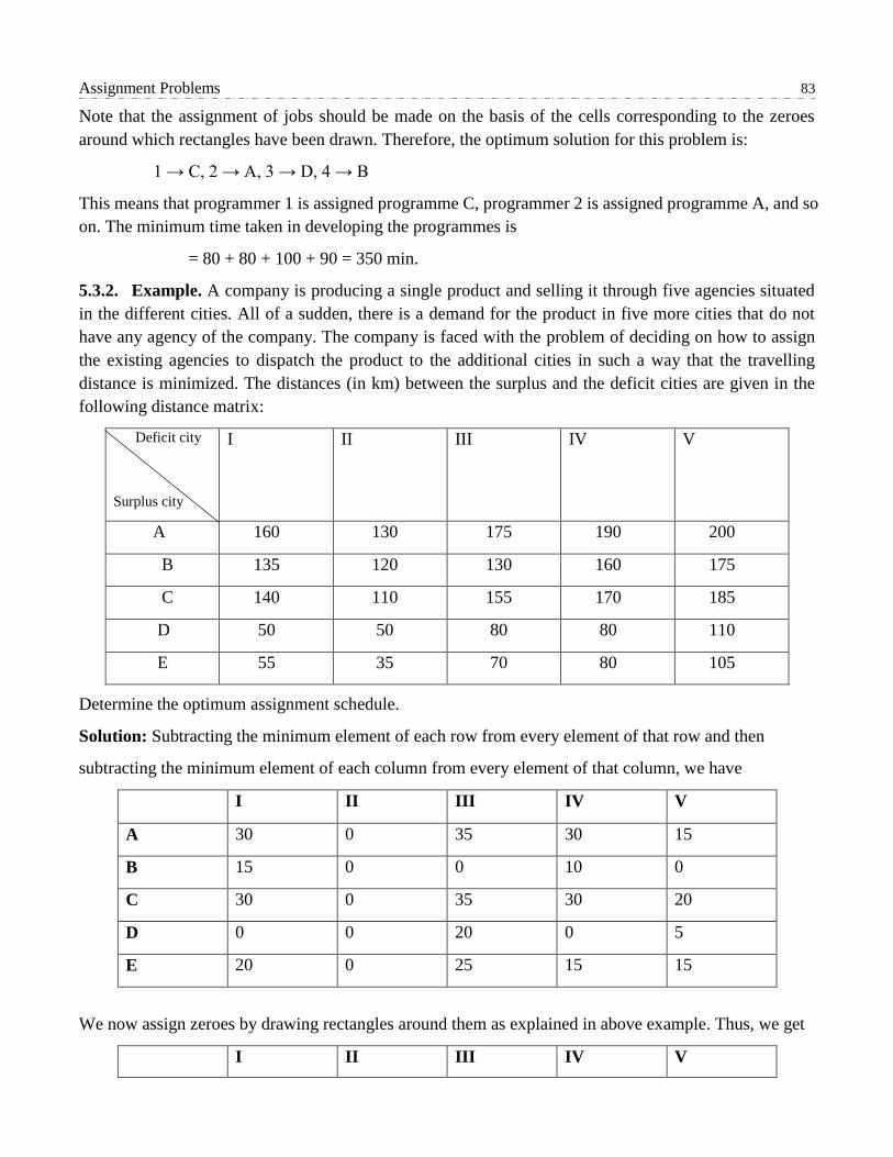
Assignment Problems 83
Note that the assignment of jobs should be made on the basis of the cells corresponding to the zeroes
around which rectangles have been drawn. Therefore, the optimum solution for this problem is:
1 → C, 2 → A, 3 → D, 4 → B
This means that programmer 1 is assigned programme C, programmer 2 is assigned programme A, and so
on. The minimum time taken in developing the programmes is
= 80 + 80 + 100 + 90 = 350 min.
5.3.2. Example. A company is producing a single product and selling it through five agencies situated
in the different cities. All of a sudden, there is a demand for the product in five more cities that do not
have any agency of the company. The company is faced with the problem of deciding on how to assign
the existing agencies to dispatch the product to the additional cities in such a way that the travelling
distance is minimized. The distances (in km) between the surplus and the deficit cities are given in the
following distance matrix:
Deficit city
Surplus city
I II III IV V
A 160 130 175 190 200
B 135 120 130 160 175
C 140 110 155 170 185
D 50 50 80 80 110
E 55 35 70 80 105
Determine the optimum assignment schedule.
Solution: Subtracting the minimum element of each row from every element of that row and then
subtracting the minimum element of each column from every element of that column, we have
I II III IV V
A 30 0 35 30 15
B 15 0 0 10 0
C 30 0 35 30 20
D 0 0 20 0 5
E 20 0 25 15 15
We now assign zeroes by drawing rectangles around them as explained in above example. Thus, we get
I II III IV V

84 Operations Research Techniques
A 30 0
35 30 15
B 15 0 0
10 0
C 30 0 35 30 20
D 0
0 20 0 5
E 20 0 25 15 15
Since the number of assignments is less than number of rows (or columns), we proceed from step 5
onwards of the Hungarian method described as follows:
i. We mark (√ ) the rows in which the assignment has not been made . These are the 3rd& 5th
row.
ii. We mark (√ ) the columns which have zeroes in the marked rows . This is the 2nd column.
iii. We mark (√ ) the rows which have assignments in marked columns . This is the 1st row.
iv. Again we mark (√ ) the columns which have zeroes in the newly marked row . This is the 2nd
column (which has been already marked).
There is no other such column. So, we have
I II III IV V
A 30 0
35 30 15 √
B 15 0 0
10 0
C 30 0 35 30 20 √
D 0
0 20 0 5
E 20 0 25 15 15 √
√
We draw straight lines through unmarked rows and marked columns as follows:
I II III IV V
A 30 0
35 30 15 √
B 15 0 0
10 0
C 30 0 35 30 20 √
D 0
0 20 0 5
E 20 0 25 15 15 √
√
We proceed as follows, as explained in the step 6 of the Hungarian method:
1) We find the smallest element in the matrix not covered by any of the lines. It is 15 in this case.
2) We subtract the number ‘15’ from all uncovered elements and add it to the elements at the intersection
of the two lines.

Assignment Problems 85
3) Other elements covered by the lines remain unchanged. Thus, we have
I II III IV V
A 15 0 20 15 0
B 15 15 0 10 0
C 15 0 20 15 5
D 0 15 20 0 5
E 5 0 10 0 0
We repeat steps 1 to 4 of the Hungarian method and obtain the following matrix:
I II III IV V
A 15 0 20 15 0
B 15 15 0
10 0
C 15 0
20 15 5
D 0
15 20 0 5
E 5 0 10 0
0
Since each row and each column of this matrix has one and only one assigned 0, we obtain the optimum
assignment schedule as follows:
A → V, B → III, C → II, D → I, E→ IV
Thus, the minimum distance is 200+130+110+50+80 = 570 km.
5.3.3. Exercise. A solicitor’s firm employs typists on an hourly piece – rate basis for their daily work.
There are five typists for service and their charges and speeds are different. According to the contract, only
one job is given to one typist. Find the least cost allocation for the following data:
P Q R S T
A 85 75 65 85 75
B 90 180 66 90 78
C 75 66 57 75 69
D 80 72 60 80 72
E 76 64 56 72 68
Answer. Applying the Hungarian method of solving an assignment problem, we finally get
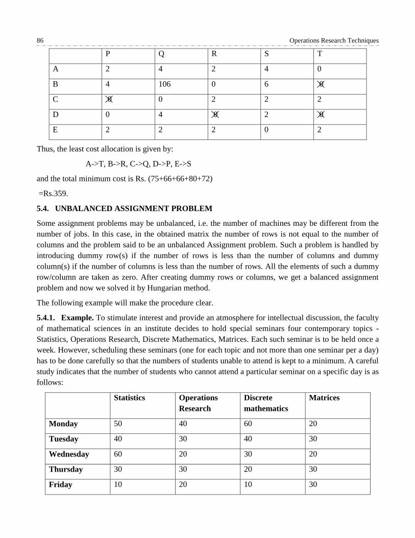
86 Operations Research Techniques
P Q R S T
A 2 4 2 4 0
B 4 106 0 6 0
C 0 0 2 2 2
D 0 4 0 2 0
E 2 2 2 0 2
Thus, the least cost allocation is given by:
A->T, B->R, C->Q, D->P, E->S
and the total minimum cost is Rs. (75+66+66+80+72)
=Rs.359.
5.4. UNBALANCED ASSIGNMENT PROBLEM
Some assignment problems may be unbalanced, i.e. the number of machines may be different from the
number of jobs. In this case, in the obtained matrix the number of rows is not equal to the number of
columns and the problem said to be an unbalanced Assignment problem. Such a problem is handled by
introducing dummy row(s) if the number of rows is less than the number of columns and dummy
column(s) if the number of columns is less than the number of rows. All the elements of such a dummy
row/column are taken as zero. After creating dummy rows or columns, we get a balanced assignment
problem and now we solved it by Hungarian method.
The following example will make the procedure clear.
5.4.1. Example. To stimulate interest and provide an atmosphere for intellectual discussion, the faculty
of mathematical sciences in an institute decides to hold special seminars four contemporary topics -
Statistics, Operations Research, Discrete Mathematics, Matrices. Each such seminar is to be held once a
week. However, scheduling these seminars (one for each topic and not more than one seminar per a day)
has to be done carefully so that the numbers of students unable to attend is kept to a minimum. A careful
study indicates that the number of students who cannot attend a particular seminar on a specific day is as
follows:
Statistics Operations
Research
Discrete
mathematics
Matrices
Monday 50 40 60 20
Tuesday 40 30 40 30
Wednesday 60 20 30 20
Thursday 30 30 20 30
Friday 10 20 10 30

Assignment Problems 87
Find an optimal schedule for the seminars. Also fine the number of students who will be missing at least
one seminar.
Solution. Here the number of rows is 5 and the number of columns is 4. Therefore, the given
assignment problem is unbalanced. As the number of columns is one less than the number of rows, we
introduce one dummy column to convert the given assignment problem into a balanced problem. The
number of students in each cell of this column is taken as zero. Thus, the problem takes the following
form:
Statistics Operations
Research
Discrete
mathematics
Matrices Dummy
Monday 50 40 60 20 0
Tuesday 40 30 40 30 0
Wednesday 60 20 30 20 0
Thursday 30 30 20 30 0
Friday 10 20 10 30 0
Now, on applying the Hungarian method (Steps 1 to 4), we get
Statistics Operations
Research
Discrete
mathematics
Matrices Dummy
Monday 40 20 50 0
0
Tuesday 30 10 30 10 0
Wednesday 50 0
20 0 0
Thursday 20 10 10 10 0
Friday 0
0 0 10 0
Since the number of assigned zeroes < number of rows, we apply Step 5 of the Hungarian method and
draw the minimum number of horizontal/ vertical lines that cover all the zeros as shown in the following
table:
Statistics Operations
Research
Discrete
mathematics
Matrices Dummy
Monday 40 20 50 0
0
Tuesday 30 10 30 10 0
Wednesday 50 0
20 0 0
Thursday 20 10 10 10 0
Friday 0
0 0 10 0
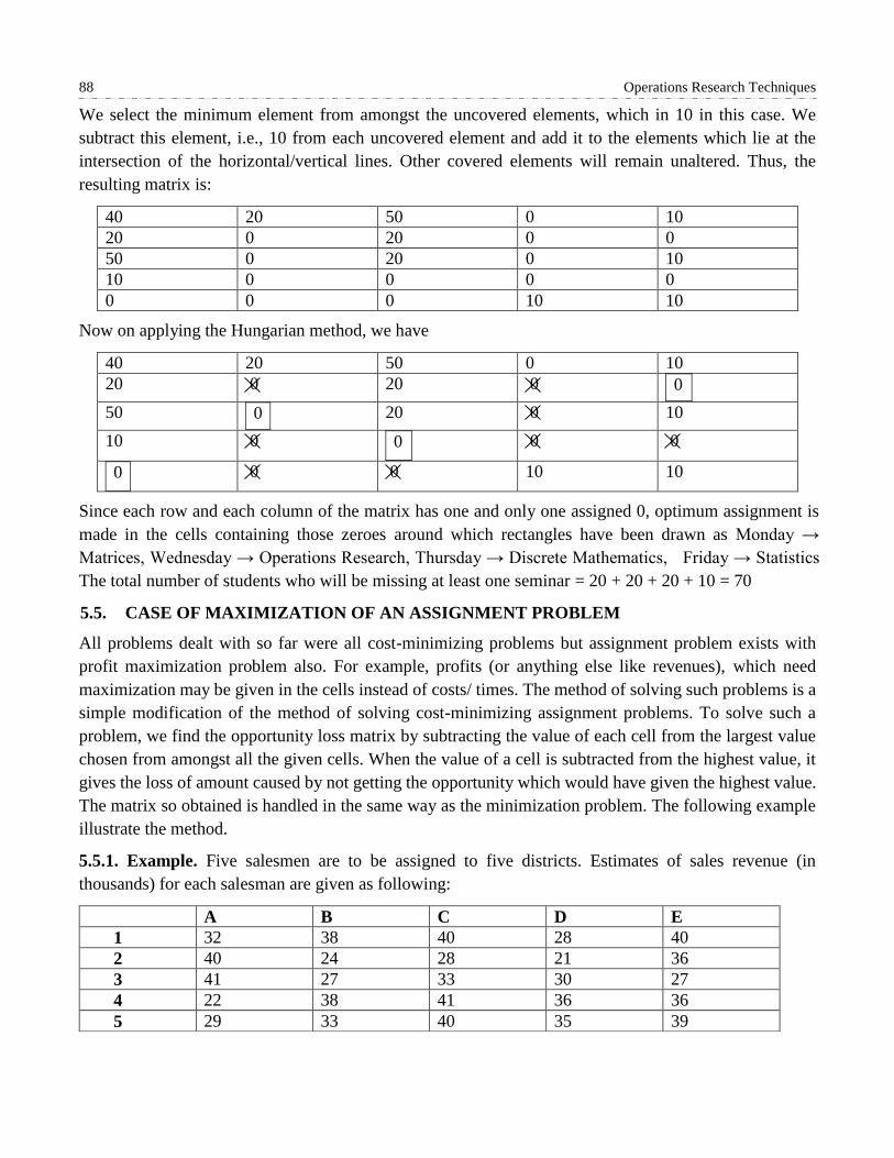
88 Operations Research Techniques
We select the minimum element from amongst the uncovered elements, which in 10 in this case. We
subtract this element, i.e., 10 from each uncovered element and add it to the elements which lie at the
intersection of the horizontal/vertical lines. Other covered elements will remain unaltered. Thus, the
resulting matrix is:
40 20 50 0 10
20 0 20 0 0
50 0 20 0 10
10 0 0 0 0
0 0 0 10 10
Now on applying the Hungarian method, we have
40 20 50 0 10
20 0 20 0 0
50 0
20 0 10
10 0 0
0 0
0
0 0 10 10
Since each row and each column of the matrix has one and only one assigned 0, optimum assignment is
made in the cells containing those zeroes around which rectangles have been drawn as Monday →
Matrices, Wednesday → Operations Research, Thursday → Discrete Mathematics, Friday → Statistics
The total number of students who will be missing at least one seminar = 20 + 20 + 20 + 10 = 70
5.5. CASE OF MAXIMIZATION OF AN ASSIGNMENT PROBLEM
All problems dealt with so far were all cost-minimizing problems but assignment problem exists with
profit maximization problem also. For example, profits (or anything else like revenues), which need
maximization may be given in the cells instead of costs/ times. The method of solving such problems is a
simple modification of the method of solving cost-minimizing assignment problems. To solve such a
problem, we find the opportunity loss matrix by subtracting the value of each cell from the largest value
chosen from amongst all the given cells. When the value of a cell is subtracted from the highest value, it
gives the loss of amount caused by not getting the opportunity which would have given the highest value.
The matrix so obtained is handled in the same way as the minimization problem. The following example
illustrate the method.
5.5.1. Example. Five salesmen are to be assigned to five districts. Estimates of sales revenue (in
thousands) for each salesman are given as following:
A B C D E
1 32 38 40 28 40
2 40 24 28 21 36
3 41 27 33 30 27
4 22 38 41 36 36
5 29 33 40 35 39

Assignment Problems 89
Find the assignment pattern that maximizes the sales revenue.
Solution. Since we are to maximize the sales revenue, we need to convert it into minimization form
before applying the Hungarian method. For this, we obtain the opportunity loss matrix by subtracting
every element in the given table from the largest element is 41. Thus, we obtain the following
opportunity loss matrix:
9 3 1 13 1
1 17 13 20 5
0 14 8 11 4
19 3 0 5 5
12 8 1 6 2
Now, we apply the Hungarian method (Steps 1 to 4) and finally obtain the following result matrix:
A B C D E
1 8 0
0 7 0
2 0
14 12 14 4
3 0 12 8 6 4
4 19 1 0
0 5
5 11 5 0 0
1
Since the number of assigned zero is less than the number of rows, we apply Step 5 of the Hungarian
method and draw the minimum number of horizontal/vertical lines that cover all the zeroes as shown in
the following table:
A B C D E
1 8 0
0 7 0
2 0
14 12 14 4 √
3 0 12 8 6 4 √
4 19 1 0
0 5
5 11 5 0 0
1
√
Let us now, select the minimum element from amongst the uncovered elements, which is 4 in the case.
We subtract the element 4 from each of the uncovered elements and add it to the elements which lie at the
intersection of the horizontal and vertical lines. Other covered elements remain unaltered. Then applying
the Hungarian method to the resulting matrix. We get
A B C D E
1 12 0
0 7 0
2 0
10 8 10 0
3 0 8 4 2 0
4 23 1 0
0 5
5 15 5 0 0
1

90 Operations Research Techniques
Since the number of assigned zeroes is equal to the number of rows, the optimum assignment has been
attained and is given as
1 → B, 2 → A, 3 → E, 4 → C, 5 → D
Thus, the maximum sales revenue = 38+ 40 +37 +41 +35 thousand rupees
= 191 thousand rupees.
5.6. TRAVELLING SALESMAN PROBLEM
Consider a travelling salesman who has to visit a certain number of cities allotted to him. He wishes to
visit each city once and only once and arrive back in the city from where he started. He knows the distances
(or cost or time) of journey between every pair of cities, and he wishes to determine the tour schedule that
represents the least distance/cost/time. Such type of problems can be solved by the assignment algorithm.
The difference between a travelling salesman and assignment problem is that in an assignment problem,
different destinations are assigned to different sources but in a travelling salesman problem, a destination
is assigned to a source. Then this destination becomes another source to which we assign another
destination, which in turn becomes another source, and so on. Let us explain this point further with the
help of an example.
5.6.1. Example: A travelling salesman has to visit five cities. He wishes to start from a particular city,
visit each city once and then return to his starting point. The travelling times for each city from a particular
city is given below
To
From
A B C D E
A ∞ 5 8 4 5
B 5 ∞ 7 4 5
C 8 7 ∞ 8 6
D 4 4 8 ∞ 8
E 5 5 6 8 ∞
What is the sequence of visits of the salesman so that the total travelling time is minimized?
Solution: Appling the Hungarian method to this problem, we get
A B C D E
A ∞ 0 2 0
0
B 0
∞ 1 0 0
C 2 1 ∞ 3 0
D 0 0
3 ∞ 4
E 0 0 0
4 ∞
As per the above assignment, the salesman should travel from A to D, D to B , B to A i.e., A→D→B→A.
The above solution is not a complete solution of the travelling salesman problem as the salesman returns
to A without travelling through all the cities.so we proceed as follows.
Since the assignment of zeroes has not given the solution of the travelling salesman problem, we bring the
next minimum non-zero element into the solution. Thus, we obtain the next best solution by bringing 1

Assignment Problems 91
into the solution. had there not been 1 in any cell, we would have taken the minimum, but greater than 1
value from amongst all the values of the tables. here we have 1and it appears in two places in this
problem.one of these is chosen arbitrarily. let us choose the cell (B, C) and from a rectangle around the
values in this cell and cross out the zeroes in its row and column. now we apply the Hungarian method for
the assignment of zeroes. Thus, we have
A B C D E
A ∞ 0 2 0
0
B 0 ∞ 1
0 0
C 2 1 ∞ 3 0
D 0
0 3 ∞ 4
E 0 0
0 4 ∞
Alternatively, we get
A B C D E
A ∞ 0 2 0 0
B 0 ∞ 1 0
0
C 2 1
∞ 3 0
D 0
0 3 ∞ 4
E 0 0 0
4 ∞
In the case of the first alternative, the optimum assignment is A→D→A, but this is not the solution of the
travelling salesman problem.
In the case of the second alternative, the optimum assignment is
A→E→C→B→D→A
This is the complete solution for the problem as starting from as the salesman returns to A visiting all the
other cities. The minimum time taken by him to travel to all the cities is 5+6+7+4+4=26hrs.
5.6.2. Exercise. Solve the following travelling salesman problem so as to minimize the cost per cycle:
To
From
A B C D E
A ∞ 3 6 2 3
B 3 ∞ 5 2 3
C 6 5 ∞ 6 4
D 2 2 6 ∞ 6
E 3 3 4 6 ∞
What is the sequence of visits of the salesman so that travelling time is minimized?
Answer. Applying the Hungarian method of solving an assignment problem, we reduce the cost matrix
and make assignments in rows and columns having single zeroes.

92 Operations Research Techniques
A B C D E
A ∞ 1 3 0
1 √
B 1
∞ 2 0 1 √
C 2 1 ∞ 2 0
D 0 0
3 ∞ 4
E 0 0 0
3 ∞
√
Now, we draw the minimum number of lines to cover all the zeroes. Then we subtract the lowest element
from all the elements not covered by any of lines and add the same at the intersection of two lines. We
have
A B C D E
A ∞ 0 2 0
0 √
B 0
∞ 1 0 0 √
C 2 1 ∞ 3 0
D 0 0
3 ∞ 4
E 0 0 0
4 ∞
√
As per the above assignment, the salesman should travel from A to D, D to B, B to A,
i.e., A→D → B → A.
The above solution is not a complete solution of the travelling salesman problem as the salesman returns
to A without travelling through all the cities. So, we proceed as follows:
Since the assignment of zeroes has not given the solution of the travelling salesman problem, we bring the
next minimum non-zero element in the solution.
Thus, we obtain the next best solution by bringing 1 into the solution. Had there not been 1 in any cell,
we could have taken the minimum, but greater than 1 value from amongst all the values of the table. Here,
we have 1 and it appears in two places in this problem. one of these is chosen arbitrarily. Let us choose
the cell (B, C) and form a rectangle around the value in this cell and cross out the zeroes in its row and
column. Now we apply the Hungarian method for the assignment of zeroes. Thus, we have
A B C D E
A ∞ 0 2 0
0
B 0 ∞ 1
0 0
C 2 1 ∞ 3 0
D 0
0 3 ∞ 4
E 0 0
0 4 ∞

Assignment Problems 93
Alternatively, we get
A B C D E
A ∞ 0 2 0 0
B 0 ∞ 1 0
0
C 2 1
∞ 3 0
D 0
0 3 ∞ 4
E 0 0 0
4 ∞
In this case of the first alternative, the optimum assignment is A→D→A, but this is not the solution of the
travelling salesman problem.
In this case of the second alternative, the optimum assignment is
A→E→C→B→D→A, i.e., 3 + 4 + 5 + 2 + 2 = 16 hr
5.7. CHECK YOUR PROGRESS
1. Define an assignment problem.
2. Explain the difference between a transportation problem and assignment problems.
3. Explain step by step procedure of Hungarian method to solve the assignment problem.
4. What is an unbalanced assignment problem?
5. Explain briefly travelling salesman problem.
5.8. SUMMARY
In this chapter, we have observed that an assignment problem may be considered as a special type of
transportation problem in which the capacity of each of the sources as well as the requirements of each of
the destination is taken as 1.In an assignment problem, the given matrix must necessarily be a square
matrix , which is not the condition for a transportation problem . Such problem is solved as Hungarian
method, which is shorter and easy compared to any other method of finding the optimal solution. We have
discussed the concept of unbalanced transportation problem; such problem is handled by introducing
dummy rows/columns. In last, we have introduced travelling salesman problem.

6 QUEUEING THEORY
Structure
6.1. Introduction.
6.2. Basic Concepts of Queueing Theory.
6.3. Fundamental Structure of a Queueing System.
6.4. Operating Characteristics of a Queueing System.
6.5. M/M/1 or M/M/1: ∞/FCFS Queueing Model.
6.6. Check Your Progress.
6.7. Summary.
6.1. INTRODUCTION
Queueing or waiting in a line is a common situation occurring in everyday life. We wait in queues in ticket
booths, bus stops, post offices, banks, traffic lights and so on.We can think of many more situations. In
general, a queue is formed when there are customers who require some sort of services and the queuing
problem is identified by the presence of a group of customers who arrive randomly to receive some service.
The customer may be a person, machine, vehicle or anything else which requires service. The objective
of a queuing model is to find out the optimum service rate and the number of servers so that the average
cost of being in queuing system and the cost of service are minimized.
The objective of a queueing system is to find ways of reducing the time spent in waiting by the customer
and at the same time optimizing the cost to the service provider. Sometimes Queueing Theory, also

Queueing Theory 95
reference as the waiting line theory. It was developed in 1909 when A.K. Erlang made an effort to analyses
telephone traffic congestion. It can be applied to wide variety of operational situations whenever
customer’s expectations do not match with objectives of servers due to one’s inability to predict accurately
the arrival and service time of customers. The purpose of queueing analysis is to provide information to
evaluate an acceptable level of service and service capacitysince providing too much service capacity is
costly (because of employees or equipment). In fact, providing too little service capacity is also costly.
In this Chapter, we discuss the concepts of stochastic processes, Poisson process and birth -death process.
We explain the basic component, fundamental structure and operating characteristics of a queueing
system. Also, we describe the M/M/1, queueing models.
6.1.1. Objectives. The objective of these contents is to provide some important concepts/results to the
reader like:
Poisson and birth-death process.
Fundamental structure and operating characteristics of a queueing system.
M/M/1 Queueing Model.
6.2. BASIC CONCEPTS OF QUEUEING THEORY
For studying queueing systems, one should be familiar with the probability theory, specially the concept
of random variable and its probability distribution such as Poisson distribution, Exponential distribution
Let us have a glance on some basic definitions.
Consider an experiment whose outcome is not uniquely determined. In such a situation an observed
outcome of the experiment is one from a set of possible outcomes.
Sample point: An outcome of an experiment is called a sample point.
Sample Space: The set of all possible outcomes of a random experiment is called sample space.
Events: Subsets of the sample space are called events.
Random Variable: A random variable is a function that associates a point of the sample space with a real
number.
Random Process/Stochastic Process: A random process or stochastic process is a family (or collection)
of random variables.
For example, if a die with six faces numbered 1, 2… 6 is thrown, the set S is a sample space where the set
of all possible outcomes is S= {1, 2, 3, 4, 5, 6}. A function X that assigns to an outcome or sample point,
the number written on it, is the random variable. The event that an odd number is observed corresponds
to the set {1, 3, 5} which is a subset of S.
Let us take more examples of stochastic process.
i) If n≥1, Suppose Xn is the outcome of the nth throw. Then {Xn, n≥1} is a collection of random
variables, such that for a distinct value of n, one gets a distinct random variable Xn. The sequence
{Xn, n≥1} constitutes a random (stochastic) process called the Bernoulli process.

96 Operations Research Techniques
ii) Let Xn represents the number of sixes in the first n throws. For each value of n=1, 2, …, we get a
distinct Binomial random variable. The sequence Xn:{ Xn, n≥1}, which gives a collection of
random variables, is a random or stochastic process.
iii) Suppose a telephone call is received at switchboard. Let Xt be the random variable, which
represents the number of incoming calls in an interval (0, t). Then Xt is a random variable and the
family {Xt, t ɛ T} constitutes a stochastic process, where T is the interval 0≤t≤∞.
6.2.1. Poisson Process
Suppose X(t) represent the maximum temperature at a particular place. Here we deal with discrete state,
continuous time stochastic processes. The Poisson process is one of the representatives of this type of
stochastic processes. The Poisson process may be explain as follows:
Let E be a random event such as (i) incoming telephone calls at a switchboard, (ii) arrival of patients for
treatment at a clinic, (iii) occurrence of accidents at a certain place.
We consider the total number N(t) of occurrences of an event E in an interval of time ‘t’. Suppose Pn(t) is
the probability that the random variable N(t) assumes the value n, i.e.,
Pn(t) = P[N(t)=n] .....1.
For n=0, 1, 2, 3.......... We have,
∑ P(t) = 1, for each fixed t .∞𝑛=0 . ......2
We can thus say from equation (2) that Pn(t) is a probability mass function of the random variable N(t)
and the family of random variables [Nt, t> 0] is a stochastic process. From our earlier discussion, you may
understand that this family is continuous parameter (in this case, time) stochastic process with a discrete
state space. This is called a Poisson process. Under certain conditions, N(t) follows a Poisson distribution
with mean 𝜆𝑡 (𝜆 is being constant). This holds for most practical situations.
6.2.1.1. Assumptions in Poisson Process
Events must be independent, in other words the number of the customers which is arrive in
disjoint time intervals are statistically independent e.g. the number of goals scored by a team
should not make the number of goals scored by another team more or less likely and the mean
number of goals scored is assumed to be the same for all teams.
The probability of two events occurring between time t and t + Δ𝑡is 0(Δ(t)), i.e. negligible.
Thus.,
P0(∆𝑡)+P1(∆𝑡)+0(∆𝑡)=1
The probability that event E occurs between time t and ∆𝑡 is equal to 𝜆∆𝑡+ 0(∆)t). Thus, P1
(∆𝑡) = 𝜆∆𝑡+0(∆𝑡),
Under the assumptions stated above, N(t) follows a Poisson distribution with mean 𝜆𝑡, i.e.,Pn(t) is given
by
Pn(t)=e-λt(λt)n
𝑛! n=0,1,2,3,........

Queueing Theory 97
To formulate a queueing model, we have to specify the assumed form of the probability distributions of
both inter arrival times and service e times. You have learnt that inter- arrival times follow the Poisson
distribution. Similarly, most of the times, the service times in a queueing system follow the exponential
distribution. Hence, the exponential distribution is the most important distribution in queueing theory
6.2.2. Markov Process
Around the beginning of the 20th century, the methodology discussed here was developed by the Russian
mathematician. A.A. Markov. The Markov Process forms a sub-class of the set of all random processes.
It is a sub class with enough simplifying assumptions to make them easy to handle.
A stochastic (or random) process is called a Markov process if the occurrence of a future state depends on
the immediately preceding state and only on it. If, for all tn, tn-1, ................,t0, satisfying tn>tn-1 >.....t0and
non- negative integer j, the family of random variables {X(t), t≥ 0} is said to be a Markov process if it
satisfy the Markovian property:
P[X(tn)=jn/X(tn-1)=jn-1,........, X(t0)=j0]=P[X(tn)=jn/X(tn-1)=jn-1],
The process has the Markov property and is called a continuous time Markov process.
6.2.3. Birth and Death Process
The arrival process assumes that the customers arrive at the queueing system and never leave it. Such a
system is known as pure birth process. On the other hand, the departure process assumes that no customer
joins the system while service is continued for those who are already in the system. If at time t=0, N is
greater than or equal to one i.e. at starting time number of customers is N. Since service is being provided
at the rate of , therefore customers leave the system at the rate of after being serviced. This type of
process is known as pure death process.
Let the state at time t would correspond to the number of arrivals by time t. 𝑃𝑛(𝑡) denotes the probability
that there are n customers in the system at any time t, both waiting and being served. Arrivals can be
considered as births. If the system is in state 𝐸𝑛 and arrival occurs, the state is changed to 𝐸𝑛+1. Similarly,
a departure can be looked upon as death. A departure occurring while the system is in state 𝐸𝑛 changes
the system to the state 𝐸𝑛−1.This type of process is generally referred to as a birth – death process.
6.2.3.1. Assumptions in the Birth-Death Process
The assumptions of the birth-death process are as follows:
If the system is in state 𝐸𝑛, the current probability distribution of the time t until the next arrival
(birth) is exponential with parameter𝜆𝑛, where n = 0, 1, 2, ... .
If the system is in state𝐸𝑛, the current probability distribution of the time t until the next
departure or service completion (death) is exponential with parameter 𝜇𝑛,where n = 0, 1, 2,….
Only one birth or death can occur in a small interval of time, i.e.,Δ𝑡.

98 Operations Research Techniques
6.3. FUNDAMENTAL STRUCTURE OF A QUEUING SYSTEM
Queuing theory is related with the mathematical study of queues or waiting lines, a queue is formed when
there are customers who require some sort of services and the current demand for a service exceeds the
current capacity to provide the service.
Generally, the customer’s arrival and their service time are not known in advance or can’t be predicted
accurately. Since arrival-departure process are random. So, queuing models developed to reduce waiting
time/excessive costs and work for maintaining balance between service capacity and waiting time.
A simple queuing system can be described as follows:
1. Input or arrival process of customers
2. Service mechanism (or process)
3. Queue discipline
The fundamental structure of a queueing system shown in the figure given below
Now we explain all the components of queueing system.
1. Input or Arrival Process of Customers
The rate at which the customers arrive at the service facility is determined by the arrival process. An
input/arrival process can be defined completely by its size, the arrival time distribution, and the attitude
of the customers. We describe these, in brief.
i) Size: It may be finite or infinite according as the arrival rate is affected or not affected by the
number of customers in the service system.
ii) The arrival time distribution: Mostly, the arrival time distribution is approximated by Poisson
distribution.
iii) Customer or arrivals behavior:
A customer who stay in the system until served no matter how much he has to wait for
service. Such a customer is called Patient Customer.
The customer who wait for a certain time in the queue and leave the system without
getting service. This kind of customer is known as impatient or reneging behavior.
If a customer before joining the system get discouraged by seeing the number of
customers already in the queue is too large and does not join the queue. This behavior of
the customer is called Balking behavior.
Input
SourceQueueing Process
Service Process
Output
Source

Queueing Theory 99
Customers who move from one queue to another because they think that their queue is
moving slower, the behavior of the customer is known as queue jockeying.
Remark: Generally, it is assumed that the customers arrive into the system one at a time. But, sometimes,
customers may arrive in groups and such arrival is called Bulk arrival.
2. Service Mechanism (or Process)
Service time distributions are generally exponential distributions. It may be any one of the following types:
1. Single channel facility
2. One queue-several station facilities
3. Several queues-one service station
4. Multi-channel facility and
5. Multistage channel facility
3. Queue Discipline
Queue discipline is the order or the manner in which the service station selects the next customer from the
waiting line to be served. There are many ways in which a customer to be selected for service. Some of
these are described as follows:
i) FIRST IN, FIRST OUT (FIFO) or in other words First Come First Served (FCFS);
ii) Last in First Out (LIFO); and
iii) Service in Random Order (SIRO)
Throughout the chapter, we consider the FCFS queue discipline.
6.4. OPERATING CHARACTERISTICS OF A QUEUEING SYSTEM
For studying queuing system, we have to set up a set of equations. We have to solve these equations to
determine the operating characteristics (or performance measures). There are two types of solutions of
these equations: (i) Transient (ii)Steady state.
Transient solutions: The time dependent solutions are known as transient solutions.
Steady state solutions: These solutions are independent of time and represent the probability of the
system being in a particular state in the long run.
Note: Here we shall be analysing the system under the steady state condition.
6.4.1. Operating characteristics/ Performance Measures
Performance Measures of a queuing system are determined by two statistical properties, namely, the
probability distribution of inter-arrival times and the probability distribution of service times.
Some of the operating characteristics/performance measures of any queueing system that are of general
interest for analysing the system are listed below:

100 Operations Research Techniques
1. Ls: The average number of customers in the queuing system (those waiting to be served and those being
served).
2. Ws:The average time each customer spends in the queuing system from entry into the queue to
completion of the service (the time spent waiting in the queue and during the service).
3. Lq: The average number of customers in the queue waiting to get service (this excludes customers
undergoing service).
4. Wq: The average time each customer spends in the queue waiting to get service (this excludes customers
time spent during the service).
5. Service idle time: The relative frequency with which the service system is idle.
Now we describe the equations for each of the operating characteristics listed above under steady state
solutions. By definition of expectation, we have
1
s n
n
L E n nP
(Expected number of customers in the system) (1)
1
q n
n C
L n c P
(Expected number of customers in queue) (2)
where there are c parallel servers so that c customers can be served simultaneously with λ arrival
rates for those who join the system, we have
s sL W (3)
and
q qL W (4)
If is the service rate, the expected service time is 1
and we have
1
s qW W
(5)
Where, sW denotes expected waiting time in system and qW represents expected waiting time in queue
Multiplying both sides of equation (5) with , we get
s qW W
s qL L
(By (3) and (4)) (6)
6.4.2. Classification of Queueing Models
Generally, queueing models are described by five symbols such as a/b/c: d/e or a/b/c/d/e. The first symbol
‘a’ describes the arrival process. The second symbol ‘b’ describes the service time distribution. The third

Queueing Theory 101
symbols ‘c’ stands for the number of servers. The symbols ‘d’ and ‘e’ stand for the system capacity and
queue discipline respectively.
First three symbols i.e. a/b/c in the above notation were described by D. Kendall in 1953. Later, A. Lee in
1966 added the fourth (d) and fifth (e) to the Kendall notation.
Remark: The fifth symbol (e) from the notation can be omitted if the system has FCFS queue discipline
and for this case it can be described as a/b/c/d. Moreover, if the system has infinite capacity with FCFS
queue discipline then we can use simply a/b/c or a/b/c: /FCFS for describing the queueing system.
Note: If arrivals follow Poisson distribution and departures follow exponential distribution, symbol M is
used in place of ‘a’ and ‘b’ e.g. suppose there is a single server then we can use the notation M/M/1(here
we consider infinite capacity and FCFS queue discipline).
6.5. M/M/1 OR M/M/1: ∞/FCFS QUEUEING MODEL
This model deals with a queueing system having a single server channel and no limit on system capacity
with Poisson input and exponential distribution for services while the customers are served on a “First
Come First Served” basis. For the given model, arrivals follow Poisson distribution and hence inter-arrival
times have an exponential distribution. The service time for this model follows an exponential distribution.
If and denote the average arrival rate and average service rate respectively then 1/ 1/and show
mean arrival time and mean service time correspondingly. Then the ratio .
.is called the traffic
intensity or the utilisation factor. It is the measure of the degree to which the capacity of the service station
is utilised. For example, if customer arrives at a rate of 10 per minute and the service rate 20 per minute,
the utilisation of the service capacity is10
50%20
, i.e., the service facility is kept busy 50% of the time
and remains idle 50% of the time.
6.5.1. Arrival-Departure Equations for the M/M/1 Queuing Model
OR
System of Differential-Difference Equations
If 1,n the probability that the system has n customers at time t t can be expressed as:
nP t t = [{Probability of n – 1 customers in the system at time t and (1 arrival, no departure in time
t or 2 arrivals, one departure in time t or 3 arrivals, two departure in time t or …)} + {Probability
of n – 1 customers in the system at time t and (2 arrivals, no departure in time t or 3 arrivals, one
departure in time t or 4 arrivals, two departures in time t or …)} + {Probability of n – 3 customers in
the system at time t and (3 arrivals, no departure in time t or 4 arrivals, one departure in time t or 5
arrivals, two departures in time t or …)} + …] + [{Probability of n + 1 customers in the system at time
t and (1 departure, no arrival in time t or 2 departures, one arrival in time t or 3 departures, two arrivals
in time t or …)} + {Probability of n + 2 customers in the system at time t and (2 departures, no arrivals
in time t or 3 departures, one arrival in time t or …)} + {Probability of n + 3 customers in the system

102 Operations Research Techniques
at time t and (3 departures, no arrival in time t or …)} + …] + [{Probability of n customers in the system
at time t and (no arrival, no departure in time t or 1 arrival, one departure in time t or 2 arrivals, two
departures in time t or …)]
= 1 1 The terms equal tonP t t O t t O t O t
2 1 The terms equal tonP t O t t O t O t
3 The terms equal tonP t O t O t
1 1nP t t O t t O t
+ The terms equal to O t
2 1 The terms equal to OnP t O t t O t t
3 The terms equaltonP t O t O t
t O t t O t + The terms which ultimately become equal to O t
Notice that t O t , O t O t , O t O t , O t O t , t t are very small and may be
taken as equal to O t
We deal with the case n = 0 separately because there cannot be any possibility of less than zero customers.
However, in the above equation, the case of less than n customers is included.
The probability of 0(Zero)customers in the system at time t t = [{Probability of 1 customer in the
system at time t and (1 departure, no customer/arrival in time t or 2 departure, 1 arrivals in time t or
3 departures, two arrivals in time t )} + {Probability of 2 customers in the system at time t and (2
departures, no arrival in time t or 3 departures, one arrival in time t or 4 departures, 2 arrivals in time
t )} + {Probability of 3 customers in the system at time t and (3 departures, no arrival in time t or 4
departures, one arrival in time t or 5 departures, two arrivals in time t )} + …] + [{Probability of O
customers in the system at time t and (no arrival, no departure in time t or 1 arrival, one departure in
time t or 2 arrivals, 2 departures in time t )}
= 1 1P t t O t t O t + The terms which ultimately become equal to
O t
2 0 1P t t t O t + The terms which ultimately become equal to O t
3P t O t + The terms which ultimately equal to O t
1 1 nP t t O t t O t

Queueing Theory 103
OP t [{Probability of no departure which 1 as there is no customer in the system and hence
no chance of departure}
1 {t O t t O t t O t + The terms which ultimately become
equal to O t
Therefore, the arrival-departure equations for the M/M/1 Queuing model are:
1 1n n nP t t P t t O t P t t O t
nP t t O t t O t
1 1 , 1nP t t t O t n
1O OP t t P t t O t P t t O t
1 1 , 0OP t t O t n (1)
1 1n n nP t t P t t P t t
1 , 1nP t t t O t n
1 0 1OP t t P t t P t t O t (2)
Dividing equation (2) by t and taking the limit as t tends to zero, we have
1 10
limitn n
n n nt
P t t P tP t P t P t
t
1
1 1n n n nP t P t P t P t (3)
and
1
1O OP t P t P t (4)
When steady state, i.e., the equilibrium state, is reached, 1
nP t becomes independent of time, say np , and
the rate of its change with respect to time becomes zero, i.e.,
1 0nP t .
Therefore, the steady-state solution is given by
1 1 0, 1n n nP P P n
1 0P P (5)
Now, from equation (5), we have

104 Operations Research Techniques
1 1n n n nP P P P (6)
This implies that
1 1 2n n n nP P P P (changing n to n – 1)
1 2 2 3n n n nP P P P (again, changing n to n – 1)
2 3 3 4n n n nP P P P (again, changing n to n – 1)
…
…
…
2 1 1 0P P P P
But 1 0 0P P (from (5))
Therefore, 1 1n n n nP P P P
1 2n nP P
1 0 0P P
1n nP P
2nP
(∵ 1 2 1 20n n n nP P P P
3nP
2 3 2 30n n n nP P P P
0 0
times
times
n
n
nP P
n
0 0
n
nP P P
.
Since 0
1,n
n
P
it follows that
0
0 0
1 ............n
n n
n n
P P P P P

Queueing Theory 105
2
0 1 1nP HP P P
0
11
1P
P
0 1P P Where P
Therefore, the probability of n customers (units) in the system is given by
1 , 0n
nP P P n
Model → M/M/1 or M/M/1: ∞/FCFS
Probability of n customers in the system is given by
1 , 1n
nP n
Probability of zero customers (units) in the queue/system is given by 0 1P
6.5.2. Operating Characteristics or Measures of Performances of the Model M/M/1
1. The average number of customers (units) in the system is given by
0 0 0
1 1n n
s n
n n n
L E n nP n n
...(*)
Now, consider 2 3
0
0 2 3n
n
n
Let 2 3
0
2 3n
n
S n
2 3 42 3S
2 3 2 3 42 3 2 3S S
2 31S
11
S
21
S
Thus from (*), we have
2
11
11sL S

106 Operations Research Techniques
Now, is the traffic intensity or utilisation factor, where
Thus, 1
1sL
(1)
Where, denotes the average arrival rate and denote the average service rate.
2. The average queue length (Expected number of customers) is qL
And Traffic intensityq sL L
2
(2)
3. The average time an arrival spends in the system (Expected waiting time in system) is
1s
s
LW
(from (1))
Thus 1
sW
(3)
4. The average waiting time of an arrival in the queue isqW .
And
2q
q
LW
(4)
from (4), we can also obtain the relation
1
q sW W
5. The probability that the number of customers (units) waiting in the queue and the number of units
being serviced is greater than k is
1kP n k (5)
6. The probability of having a queue i.e. 01 P
Thus 01 1 1P (6)
Now, we explain the M/M/1 queuing model with the help of following examples.
6.5.3. Example. A TV repairman finds that the time spent on his job has an exponential distribution with
mean 30 minutes. If he repairs sets in the order in which these come in, and if the arrival of sets is
approximately Poisson with an average rate of 10 per 8-hour day, what is the repairman’s expected idle
time each day? How many jobs are ahead of the average set just brought in?

Queueing Theory 107
Solution: Here, we have
Arrival rate 10
8 arrivals/hr
Service rate 60
230
services/hr
∴ The probability of the repairman being idle is
0
10 1 5 31 1 1 1
8 2 8 8P
Thus, 0
3
8P .
Hence the idle time in the 8-hour day = 3
88 hours = 3 hours
Now, the average number of jobs that are ahead of the set (person) just brought in
= Average number of units in the system means who are in queue and at counter, i.e.
10
10 58 1.66610 6 3
28
sL
Thus, 1.67sL .
6.5.4. Example. Customers arrive at a window in a bank, according to a Poisson distribution with mean
10 per hour. Service time per customer is exponential with mean 5 minutes. The space in front of the
window including that for the serviced customers can accommodate a maximum of three customers. Other
customers can wait outside this space.
(a) What is the probability that an arriving customer can go directly to the space in front of the window?
(b) What is the probability that an arriving customer will have to wait outside the indicated space?
(c) How long is an arriving customer expected to wait before being served?
Solution: Here, arrival rate = 10 per hour and service rate 60
5 per hour = 12 per hour
Thus, traffic intensity 10 5
60 6
5
5
6

108 Operations Research Techniques
(a) The probability that an arriving customer can go directly to the space in front of the window i.e.
the probability of n customers in the system here 2 ≥ n ≥ 0, therefore the required probability 0 1 2P P P
25 5 5 5 5
1 1 16 6 6 6 6
1 1 5 1 25
0.426 6 6 6 36
(b) The probability that an arriving customer will have to wait outside the indicated space, i.e. the
required probability = 3 4 5P P P
0 1 21 P P P
= 1 – 0.42 = 0.58
(c) Expected waiting time before being served
qW
10
0.41712 12 10
hours
6.5.5. Exercises.
1. Customers arrive at a box office window being served by a single individual according to a Poisson
input process with a mean rate of 30 per hour. The time required to serve a customer has an exponential
distribution with a mean of 90 seconds. Find the average waiting time of a customer in the queue.
Solution. 30 3
( ) 40(40 30) 10qhrW
= 3
604 minutes = 4.5 minutes
2. A fertilizer company distributes its products by trucks loaded at its only loading station. Both
company trucks and contractor’s truck are used for this purpose. It was noticed that on an average on truck
arrived every 5 minutes and the average loading time was 3 minutes. Forty percent of the trucks belong to
the contractor. Determine the expected waiting time of contractor’s trucks per day.
Solution. The expected waiting time of contractor’s truck per day=8.64 hrs.
3. In a railway marshalling yard, goods train arrives at a rate of 36 trains per day. Assuming that
inter-arrival time follows exponential distribution and the service time distribution is also exponential with
an average of 30 minutes, calculate the following:
i. The mean line length
ii. The probability that the queue size exceeds 10.
iii. If the input increases to an average of 42 per day, what will the change in (a) and (b) be?
Solution. (i) Mean length of a system
Ls = 3 trains 1

Queueing Theory 109
(ii) Probability that the queue size exceeds 10= probability that the system size exceeds 11
i.e., P (n>11) = (0.75)12
c) Ls = ’ / μ- ’ = 42/48-42 = 7 trains
And the probability that the queue size exceeds 10 is (7/8)12
6.6. CHECK YOUR PROGRESS
1. What is Queueing Theory?
2. Explain what do you mean by Poisson process.
3. Describe birth and death process.
4. Explain briefly fundamental structure of Queueing System.
5. Write a note on operating characteristics of Queueing System.
6. Explain classification of Queueing System.
7. Derive the arrival-departure equation for M/M/1 Queueing Model.
8. State operating characteristics of M/M/1 Queueing Model.
6.7. SUMMARY
In this chapter, we have introduced the concept of queueing theory. It has been observed that for
understanding queueing system, we have to familiar with some concepts namely Stochastic Process,
Poisson Process, and Birth-Death Process along with some distributions such as Poisson distribution and
exponential distribution. We explained the basic component, fundamental structure and operating
characteristics of a queueing system. Also, we discussed the M/M/1, queueing models.

7 QUEUEING MODELS
Structure
7.1.Introduction.
7.2. M/M/C or M/M/C: ∞/FCFS Queueing Model.
7.3. M/M/1/K Queueing Model.
7.4. M/M/C/K Queueing Model.
7.5. Check Your Progress.
7.6. Summary.
7.1. INTRODUCTION
Queueing theory is the mathematical study of waiting lines or queues and considered a branch of
operations research because the results are often used when making business decisions about the resources
needed to provide a service. A queueing model is constructed for predicting queue lengths and waiting
time.
In the chapter 6, we have discussed the basic concept of queueing theory which would help us in
understanding the techniques of queueing models. We studied about the fundamental structure, operating
characteristics and classification of queueing models. Also, we described M/M/1 queueing model and its
applications. In the present chapter, we shall describe some other queueing modelswith single and multiple
servers namely M/M/C, M/M/1/k and M/M/C/k queueing models.
7.1.1. Objectives. The objective of these contents is to explain some important queueing models with
single and multiple servers to the reader such as:
M/M/C Queueing Model.

Queueing Models 111
M/M/1/k Queueing Model.
M/M/C/k Queueing Model.
7.2. M/M/C OR M/M/C: ∞/FCFS QUEUEING MODEL
This model deals with a queueing system having a multiple server channel and no limit on system capacity
with Poisson input and exponential distribution for services while the customers are served on a “First
Come First Served” basis. We consider a queue with Poisson input (having arrival rate, say, ) and with
C (1 ≤ C< ∞) parallel service channels having independently and identically distributed exponential
service time distribution, each with rate, say, .
If there are n units in the system, and n is less than C, then, in all, n channels, are busy. If there are n (≥
C) in the system, then all the C channels are busy. Thus, we have a birth death model having constant
arrival (birth) rate and state-dependent service (death) rate.
, 0,1, 2, ,
, 1, 2,n
n n C
C n C C
Hence, the steady state probability exist if
1C
and are given by
0
0
, 02
,2
n
P n Cn
P
P n CC C C
, ( ... ) ( ) .where theterm c c is repeated n c times
0
0
, 0!
,!
n
n
n C
P n Cn
P n CC C
Now, 0
1n
n
P
1 1 1
0
0 0 0
1 1! !
n n
C C C
n n n Cn n C n n
P P Pn C C
1
0
0
1! !
n n C nC
n n C
C CP
n C
, where
C

112 Operations Research Techniques
11
0
0 ! !
n n C nC
n n C
C CP
n C
11
0
1
! ! 1
n n CCC
n
C C
n C
7.2.1. Operating characteristics/Performance measures of M/M/C Model
In chapter 6, we have already defined the meaning of performances measures such as , ,L L W and Wq s q S
, here we
only evaluate mathematical expression for all these as given below:
1. q n
n C
L n C P
1
C j
j
jP
, Now put n – C = j, we get
0
1 !
c j
jj
j
PC C
0
1!
C
j
j
P
jC
0
2! 1
C
P
C
1
21 1
1 1
1 1
j j
j j
d dj
d d
2. s qL L
(Expected number of customers in the system)
3. Expected waiting time in the queue
1
q qW L
4. Expected waiting time in the system
1
s qW W
or ss
LW
The following examples illustrate M/M/C queueing Model.
7.2.2. Example. A petroleum company is considering expansion of its unloading facility at its refinery.
Due to random of variations in weather, loading delays and other factors, ships arriving at the refinery to
unload crude oil arrive at an average rate of 5 ships per week. Service rate on an average is 10 ships per
week. Assuming Poisson arrivals and exponential service distributions, find

Queueing Models 113
(a) The average time a ship must wait before beginning to deliver its cargo to the refinery;
(b) If a second birth is rented, what will be the average number of ships waiting before being unloaded?
(c) What would be the average time a ship would wait before being unloaded with two berths?
(d) What is the average number of idle berths at any specified time?
Solution: (a) Here, we have the case of M/M/1 model
5 per week, 10 per week
1
10qW
week
(b) For this case, we have M/M/2 model
Here 5 1
2 10 4C
12
0
11
12!1
4
P
1 11 1 4 3 1 9 1 3
12 8 3 2 6 6 5
0
2
1
30! 1
C
q
P
LC
(c) 150q
q
LW
week
(d) 1 0
: 1 2
:
X
P P P
Where X be the number of idle berths and probability of number of ships in the system
1 02 1.5E X PX P P
Hence 2 births are idle.
7.2.3. Example. Arrival of machinists at a tool crib are considered to be Poisson distributed at an average
rate 6 per hour. The length of time the machinists must remain at the tool crib is exponentially with average
time of 0.05 hours.
a) What is the probability that a machinist arriving at the tool crib will have to wait?
b) What is the average number of machinists at the tool crib?
c) The company will install a second tool crib when convinced that a machinist would have to spend 6
minutes in waiting and being served at the tool crib. At what rate should the arrival of machinist to the
tool crib increase to justify the addition of a second crib?

114 Operations Research Techniques
Solution. a) Here the arrival rate = 6/hr and the service rate = 20/hr
Therefore, the probability of zero customers in queue is
0P = 1 where 6
20
0P = 6 14 71 0.720 20 10
The probability that a machinist arriving at the tool crib will have to wait
= Probability that there is at least one machinist at the tool crib
= 1- Probability that there is no machinist at the tool crib
= 1- 0P = 1- 0.7 = 0.3
b) The average number of machinists at the tool crib is given by
Ls =
=
6 6
20 6 14
= 0.428
c) The company is ready to install a second tool crib when convinced that a machinist would have to spend
6 min. in waiting and being served. Let the increased arrival rate be'
.
Waiting time in the system = 6 min. = 1
10 hr.
We have 1
' =
1
10
or 1
'20 =
1
10
or 10 = 20 - '
or ' = 20 – 10 = 10/hr
The increase is, therefore, (10 – 6)/hr = 4/hr.
7.2.4. Example. A repairman is to be hired to repair machines which break down at an average rate of 3
per hour. The breakdown follows a Poisson distribution. Nonproductive time of a machine is considered
to cost 10 Rs per hour. Two repairmen have been interviewed of whom one is slow but charges less and
the other is fast but more expensive. The slow repairman charges 5 Rs per hour and services breakdown
machines at the rate of 4 per hour. The fast repairman demands 7 Rs per hour, but services breakdown
machines at an average rate of 6 per hour. Which repairman should be hired?
Solution. The data given is summarized below:
Slow/less expensive Repairman:
= 3/hr , = 4/hr , Labour cost = 5 Rs/ hr
Fast/more expensive Repairman:
= 3/hr, = 6/hr, Labour cost = 7 Rs/ hr
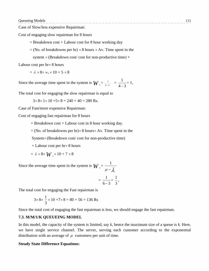
Queueing Models 115
Case of Slow/less expensive Repairman:
Cost of engaging slow repairman for 8 hours
= Breakdown cost + Labour cost for 8 hour working day
= (No. of breakdowns per hr) 8 hours Av. Time spent in the
system (Breakdown cost/ cost for non-productive time) +
Labour cost per hr8 hours
= 8 Ws 10 + 5 8
Since the average time spent in the system is sW =
1
=
1
4 3= 1,
The total cost for engaging the slow repairman is equal to
38110 +58 = 240 + 40 = 280 Rs.
Case of Fast/more expensive Repairman:
Cost of engaging fast repairman for 8 hours
= Breakdown cost + Labour cost in 8 hour working day.
= (No. of breakdowns per hr)8 hoursAv. Time spent in the
System (Breakdown cost/ cost for non-productive time)
+ Labour cost per hr8 hours
= 8sW 10 + 7 8
Since the average time spent in the system is sW =
1
= 1
6 3=
1
3,
The total cost for engaging the Fast repairman is
381
310 +78 = 80 + 56 = 136 Rs
Since the total cost of engaging the fast repairman is less, we should engage the fast repairman.
7.3. M/M/1/K QUEUEING MODEL
In this model, the capacity of the system is limited, say k, hence the maximum size of a queue is k. Here,
we have single service channel. The server, serving each customer according to the exponential
distribution with an average of customers per unit of time.
Steady State Difference Equations:

116 Operations Research Techniques
The simplest way of starting this is to treat the model as a special case of birth death process, where
, 0
0, elsewheren
n k
and n for n=1,2,3, ...
Now, following the similar arguments as given in M/M/1 model, we obtain
0 0 11 0 , 0P t t P t t P t t t n
1 11 0n n n nP t t P t t P t t P t t t ,
for n = 1, 2, …, k – 1 and
11 0 0 0k k kP t t P t t P t t x t t
11 0k kP t t P t t
Now, dividing above three equations by t and taking limit as 0,t these equations transform into
1
0 0 1P t P t P t for n = 0
1
1 1n n n nP t P t P t P t for n = 1, 2, …, k – 1
and 1
1k k kP t P t P t , for n = k
Thus, the steady-state equations are:
1 1 0,1n n nP P P n k (1)
0 1 0P P (2)
1,k kP P n k (3)
for 1 ≤ n<k, by (1) we have
1 1n n n nP P P P
1 2n nP P (on replacing n by n – 1)
…
…
…
1 0P P
Now, from (2), (3) and the above equation, we have
1 0; 0n nP P n k
1n nP P
2nP

Queueing Models 117
0 0
n
nP P
, n = 0, 1, 2, …, k
But 0
1k
n
n
P
Therefore, 0
0
1k
n
n
P
2
0 1 1kP
0 2
1
1P
k
1
1, if 1
1
1, if 1
1
k
k
1
1if 1
1
1if 1
1
n
k
nP
k
7.3.1. Operating Characteristics/Performances Measures of M/M/1/K
or M/M/1: K/FCFS Queuing Model
i. Expected number of customers in the system i.e.
0
k
s n
n
L E n nP
1
0
0
1, if 1
1
1, if 1
1
nk
kn
k
n
n
nk
1
11
1, if 1
1
11 2 3 , if 1
1
kn
kn
n
kk
But 1
1 1
k kn n
n n
dn
d

118 Operations Research Techniques
2 31
1
k
kd d
d d
1
2
1 1 1 1
1
k k kk
2 2
1 1 1
1 11 1
kk k kk k
1
21
11, if 1
1 11
, if 12
k k
k
s
k
L
k
1
1, if 1
1 1 1
, if 12
k k
k
k
k
1 1
1
1, if 1
1 1
2
k k kk
kk
k
1 1 1
1
1, if 1
1 1 1
, if 12
k k k k k
k
k k
k
1
1
1 11, if 1
1 1 1
, if 12
k kk
k
k
k
1
1
1, if 1
1 1
, if 12
k
k
k
k
ii. Expected queue length i.e.
0
1 1
1 1k k
q n n
n n
L n P nP P

Queueing Models 119
01sL P
Note: The relationships ss
LW
and
q
q
LW
as already given for model M/M/1 are not valid here. This
is because no arrivals are allowed to join the system once the maximum allowable length is reached.
However, if is replaced by 1 1 kP which is the effective rate of arrival, then
1
1,s
s q s
LW W W
Remark: For M/M/1/K model, the assumption is not necessary for deriving steady state results.
The steady-state probabilities can be obtained for also and in this case,
1
, 1, 2, ,1
nP n Nk
and
11 1, , ,
2 2 2 2 1s s q q
k kk k kL W W L
k
7.3.2. Example. At a railway station, only one train is handled at a time. The railway yard is sufficient
only for two trains to wait while others are given a signal to leave the station. Trains arrive at an average
rate of 6 per hour and the railway station can handle them on an average of 12 per hour. Assuming Poisson
arrivals and exponential service time distributions, find the steady-state probabilities for various number
of trains in the system. Also find the average waiting time of a new train coming in the system.
Solution. Here 6 per hour, 12 per hour, k = 2, 1
2
Steady-state probabilities are:
0 2 1 3
1 1 4
1 1 7P
0; 0,1, 2,n
nP n
1 4
2 7n
Now, 2
0 0
0
1 1 41 1 1
2 4 7n
n
P P P
1 4
; 0,1, 22 7
n nP n
The average waiting time of an incoming train
1
ss
LW
, where
1
1
1
1 1
k
s k
kL

120 Operations Research Techniques
3
3
11 322
1 11 12 2
3
4817 7
8
2
1 4 361 6 1
4 7 7P
4
1736 9
7
sW hours
7.4. M/M/C/K QUEUEING MODEL
In this system, the maximum size of a queue is k and the number of servers is C. For example, a car
servicing station may have only facilities for offering services to C cars at a time. However, because of
space limitation, the station can accept only k cars at any one point of time of servicing C (<k) cars.
The queuing system can be treated as a special case of the birth death process where
, 0
0, elsewheren
n k
and , 0
,n
n n C
C C n k
Hence, the steady state probabilities are given by
0
0
; 02
,
2times
n
P n Cn
PC n k
C C CC P
n C
0
/,
!
,!
n
n
n C
P C n kn
n kC C
Where, 0P is given by 0
1k
n
n
P
0 0
0 1
1! !
n n
C k
n Cn n C
P Pn C C

Queueing Models 121
1
0
0 1! !
n
nCC k
n n C
CP
n C C
1
0 1! !
n n C nC k
n n C
C C
n C
, where
C
7.4.1. Operating Characteristics/Performance Measures of the M/M/C/K Queueing Model
1. 1
k
s n
n
L nP
2. 1
k
q n
n C
L n C P
3. ss
LW
,where 1 kP
4. q
q
LW
W, where 1 kP
7.4.2. Example. A car servicing station has two bays where service can be offered simultaneously. Due
to a limitation in space, only four cars are accepted for servicing. The arrival pattern is Poisson with 12
cars per day. The service time for both the bays is exponentially distributed with 8 cars per day per
bay. Find the average number of cars in the service station, the average number of cars waiting to be
serviced and the average time a car spends in the system.
Solution. Here, 12, 8, 2C
12 3
, 42 8 4
kC
Therefore,
1
0
0 1! !
n n C nC k
n n C
C CP
n C
1
2
2 4
0 3
3 32 2
4 4
! 2!
n n
n
n nn
1
93 27 8141 22 2! 64 256
13 9 27 81
12 8 32 128
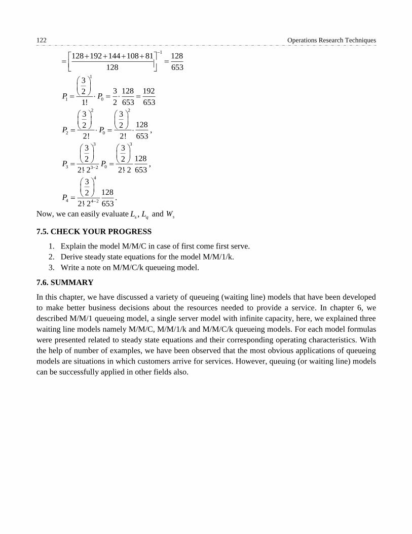
122 Operations Research Techniques
1128 192 144 108 81 128
128 653
1
1 0
3
3 128 1922
1! 2 653 653P P
2 2
2 0
3 3
1282 2
2! 2! 653P P
,
3 3
3 03 2
3 3
1282 2
2! 2 2! 2 653P P
,
4
4 4 2
3
1282
2! 2 653P
.
Now, we can easily evaluate ,s qL L and sW
7.5. CHECK YOUR PROGRESS
1. Explain the model M/M/C in case of first come first serve.
2. Derive steady state equations for the model M/M/1/k.
3. Write a note on M/M/C/k queueing model.
7.6. SUMMARY
In this chapter, we have discussed a variety of queueing (waiting line) models that have been developed
to make better business decisions about the resources needed to provide a service. In chapter 6, we
described M/M/1 queueing model, a single server model with infinite capacity, here, we explained three
waiting line models namely M/M/C, M/M/1/k and M/M/C/k queueing models. For each model formulas
were presented related to steady state equations and their corresponding operating characteristics. With
the help of number of examples, we have been observed that the most obvious applications of queueing
models are situations in which customers arrive for services. However, queuing (or waiting line) models
can be successfully applied in other fields also.
8 INVENTORY MODELS
Structure
8.1. Introduction
8.2. Meaning of Inventory Control
8.3. Economic Order Quantity (EOQ)
EOQ Model with Uniform Demand
EOQ Model with Uniform Replenishment
EOQ with Different Rates of Demands in Different Cycles
EOQ Model when Shortages are Allowed
EOQ Model with Price Breaks
8.4. Check Your Progress
8.5. Summary
8.1. INTRODUCTION
In this chapter, we shall introduce the concept of inventory and discuss different kinds of inventory
models. Inventory may be defined as a stock of idle resources of any kind having an economic value kept
for the purpose of future affairs. The term is generally used to indicate physical resources such as raw
materials, semi-finished goods used in the production process, finished products ready for delivery to
consumers, human resources such as unused labour or financial resources such as operating capital etc.
stock or order to meet an expected demand in the future.

124 Operations Research Techniques
In the present chapter, we discuss the models for inventory control known as economic order quantity
(EOQ) models. EOQ models help in deciding as to how much quantity should be kept in stock so that one
can balance the costs of holding too much stock. Here, we discuss inventory control, various factors
influencing inventory and describe models for determining the EOQ: (i)when demand is uniform; (ii)
when shortages are allowed;
(iii) when replenishment is uniform; (iv) when price breaks.
8.1.1. Objectives: The objective of these contents is to get familiar reader with the concept of inventory.
After studying this chapter, reader should be able to describe the following concepts like:
(i) Inventory Control
(ii) EOQ Model with Uniform Demand
(iii) EOQ Model with uniform replenishment
(iv) EOQ with different rates of demands in different cycles
(v) EOQ Model when shortages are allowed
(vi) EOQ Model with price breaks
8.2. MEANING OF INVENTORY CONTROL
Inventories are essential for business and maintenance of inventories costs money by way of expenses on
stores, personnel, equipment, insurance etc. Thus, excess inventories are undesirable. Therefore,
controlling the inventories in the most profitable way is the need of every business.
8.2.1. Necessity for Maintaining Inventory
Though inventory of materials is an idle sequence (since the materials lie idle and are not to be used
immediately) almost every organisation must maintain it for efficient and smooth running of its operations,
if an enterprise has no inventory of materials at all. On receiving a sales order, it will have to place order
for purchase of raw materials, wait for their receipt and then start production. The customer will thus have
to wait for a long time for the delivery of the goods and may turn to other suppliers resulting in loss of
business for the enterprise. Maintain an inventory is necessary because of the following reasons:
1. It helps in smooth and efficient running of an enterprise.
2. It provides service to the customer at a short notice timely delivery can fetch more goodwill and
order.
3. In the absence of inventory, the enterprise may have to pay high prices because of piece-wise
purchasing. Maintaining of inventory may earn price discount because of bulk purchasing.
4. It reduces product cost because there is an additional advantage of batching and long production
runs.
5. It acts as a buffer stock when raw materials are received late and so many sale orders are likely to
be rejected.

Inventory Models 125
6. Process and movement inventories (also called pipe line stocks) are quite necessary in big enterprises
where significant amounts of times are required to tranship items from one location to another.
7. Bulk purchases will entail less orders and therefore fewer clerical costs.
8. It helps in maintaining economy by absorbing some of the fluctuations when the demand for an item
fluctuates and is seasonal.
8.2.2. Factors Influencing Inventories
The major problem of inventory control is to answer two questions:
1. How much to order?
2. When to order?
These are answered by developing a model. An inventory model is based on the consideration of the main
aspects of inventory. The varieties of factors related to these are placed below:
1. Inventory related costs
Various costs associated with inventory control are often classified as follows:
(a) Purchase (or production) cost. The cost of purchasing (or producing) a unit of an item is known
as purchase (or production) cost. The purchase price will become important when quantity discounts
are allowed for purchases above a certain quantity.
(b) Ordering (or set up) cost. If any item is purchased, an ordering cost is incurred each time an order
is placed. This cost includes the following factors: administrative (paper work, telephone calls,
postage), transportation of items ordered, receiving and inspection of goods etc. If a firm produces its
own inventory instead of purchasing the same from an outside source, then production set-up costs are
analogous to ordering costs.
(c) Carrying (or holding) cost. Holding cost represents the cost of maintaining inventory in stock. It
includes the interest on capital, sent for space used for storage, insurance of stored equipment,
depreciation, taxes, etc.
(d) Shortage (or stock out) cost. The penalty cost for running out of stock (i.e. when an item cannot
be supplied on the customer’s demand) is known as shortage cost. This cost includes the loss of
potential profit through the sale of items demanded and loss of goodwill, in terms of permanent loss of
customers and its associated lost profit in future sales.
(e) Salvage cost (or selling price). When the demand for an item is affected by its quantity in stock,
the decision depends upon the underlying criterion and includes the revenue from sale of the item.
Salvage cost is generally combined with the storage cost and hence is neglected.
2. Demand: Demand is the number of units required per period and may be either known exactly or known
in terms of probabilities. Problems in which demand is known with certainty, are called deterministic
problems, whereas problems in which demand is assumed to be a random variable are called
probabilistic problems.

126 Operations Research Techniques
3. Order cycle. The time period between placement of two successive orders is referred to as an order
cycle. The order may be placed on the basis of the following two types of inventory review systems.
(a) Continuous review. The record of the inventory level is checked continuously until a specified
point (called reorder point) is reached when a new order is placed.
(b) Periodic review. In this system, the inventory levels are reviewed at equal time intervals and the
orders are placed at such levels.
4. Time horizon. The time period over which the inventory level will be controlled is referred to as time
horizon. This can be finite or infinite depending upon the nature of demand. This is also known as the
planning period over which the inventory is to be controlled. Mostly inventory planning in an enterprise
is done on annual basis.
5. Lead time. The time between placing an order and its arrival in stock is known as lead time. The lead
time can be either deterministic or probabilistic. If the lead time is zero, there is no need for placing an
order in advance. If the lead time is known and is not equal to zero and also the demand is known, then it
is required to place an order in advance-by-an amount of time equal to the lead time.
6. Re-order level. The level between maximum and minimum stock, at which the purchasing (or
manufacturing) activities must start for replenishment is known as reorder level.
7. Stock replenishment: The rate at which items are added to inventory is one of the important parameters
in inventory models. The actual replenishment of items may occur instantaneously or gradually.
Instantaneous replacement is possible when the stock is purchased from outside sources while gradual
replenishment is possible when the product is manufactured by the company.
8. Re-order quantity: This is the quantity of replenishment order. In certain cases, it is the Economic
Order Quantity.
Some notations used in the models
The notations used in the development of models are as follows:
Q = number of units ordered per order
D = demand in units of inventory pr time period
N = number of orders placed per time period
TC = total inventory cost
0C = ordering cost (or setup cost per production run) per order
pC = Carrying or holding cost per unit per period of time the inventory is held
C = Purchase or manufacturing price per unit inventory
sC = shortage cost per unit of inventory
L = lead time

Inventory Models 127
T = reorder cycle time i.e. time period between placement of two successive orders as a fractional
part of standard time horizon
pr = replenishment rate at which lot size Q is added to the inventory
8.3. ECONOMIC ORDER QUANTITY (EOQ)
‘Economic Order’ Quantity or ‘Economic lot size’ was first developed by Ford W Harris in 1913 in order
to balance costs of holding two much stock against that of ordering in small quantities too frequently.
Economic order quantity is the size of the order representing standard quality of material and is the one
for which the aggregate of the costs of procuring the inventory and costs of holding the inventory is
minimum.
8.3.1. Model I: EOQ Model with Uniform Demand
The objective of the model is to determine an optimum EOQ such that the total inventory cost is minimum.
Following assumptions are made for this model:
1. Demand D is constant and known.
2. Replenishment is instantaneous i.e. the entire order quantity Q is received at one time as soon as the
order is released.
3. Lead time is zero.
4. Purchase price or cost per unit is constant i.e. discounts are not allowed.
Carry cost hC
and ordering cost oC
are known and constant.
6. Shortage is not allowed.
Inventory
Since lead time is zero and replenishment is instantaneous safely stock is not required i.e. minimum
level is zero. Also, demand is uniform. So, the average inventory per cycle

128 Operations Research Techniques
1
2
(maximum level + minimum level)
1
2 2
QQ O
Since average inventory during any cycle period is 2
Q
, the average inventory during the entire period is
also 2
Q
.
So, carrying cost = average units in inventory × carrying cost per unit 2h
QC
Ordering cost = number of orders × ordering cost per order
oN C
o
DC
Q
Total variable inventory cost is then given by
2o h
D QTC C C
Q
Differentiating w.r.t. Q, we get
2 2
o hDC CdTC
dQ Q
2
2 3
2 oDCdTC
dQ Q
For maxima or minima,
0
dTC
dQ
i.e. 2
02
o hDC C
Q
i.e. 2
o hC D C Q
Q
i.e.
2 o
h
DCQ
C
At
2
2
2, 0o
h
DC dQ TC
C dQ

Inventory Models 129
Hence TC is minimum when
2 o
h
DCQ
C
.
∴ EOQ is given as
* 02
h
DCQ
C
Optimum number of orders placed per time period *
*
DN
Q
Minimum total variable inventory cost
*
* 22o h o h
D QC C DC C
Q r
2 demand rate ordering cost holding cost
Optimum length of time between orders
*Q
D
2 21 o o
h h
DC C
D C DC
Note: If the carrying cost is given as a percentage of average value of inventory held, then total annual
carrying cost hC may be expressed as
hC cost of one unit × inventory carrying cost in percentage = CI
Hence optimum order quantity is given by
* 2 oDCQ
CI
8.3.1.1. Example. The demand rate of a particular item is 12000 units per year. The set-up cost per run
is Rs. 350 and the holding cost is Rs. 20 per unit per month. If no shortages are allowed and the
replacement is instantaneous, determine
(i) the optimum run size,
(ii) the optimum scheduling period, and
(iii) minimum total expected annual cost.
Solution. Here, D = 12000 per year
0C = Rs. 350
hC = Rs. 0.2 per unit per month

130 Operations Research Techniques
= Rs. 2.4 per unit per year
(i) Optimum lot size
* 2 o
h
DCQ
C 2 12000 350
2.4
3500000 1870.8 1871units
(ii) Optimum scheduling period
** 1871
years =1.87 months12000
Qt
D
(iii) minimum total expected annual cost 2 o hDC C
2 12000 350 2.4
20160000 Rs. 4490
8.3.1.2. Example. The annual requirement for a product is 3000 units. The ordering cost is Rs. 100 per
order. The cost per unit is Rs. 10. The carrying cost per unit per year is 50% of
the unit cost. Find the EOQ. If a new EOQ is found by using ordering cost as Rs. 80, what would be the
further savings in cost?
Solution. Here D = 300 units per year
oC = Rs. 100
C = Rs. 10, I = 30%
hC = CI =
3010
100
= Rs. 3 per unit per year.
Optimal lot size,
* 2 2 3000 100447 units
3
o
h
DCQ
C
Total inventory cost 02 hDC C
2 3000 100 3 = Rs. 1342 per year
In the second part, we have D = 3000, oC = Rs. 100/80, hC
= Rs. 3 per unit per year
* 02 2 3000 80
2h
DCQ
C
= 400 units.
Total inventory cost 2 2 3000 80 3o hDC C
= Rs. 1200 per year

Inventory Models 131
Net savings = 1342 – 1200 = Rs. 142 per year.
8.3.1.3. Example. A company requires 1000 units per month. Order cost is estimated to be Rs. 50 per
order. In addition to Re 1.00, the carrying costs are 10% per unit of average inventory per year. The
purchase price is Rs. 10 per unit. Find the economic lot size to be ordered and the total minimum cost.
Solution. Here D = 1000 units per month
= 12000 units per year
0C = Rs. 50 per order
C = Rs. 10 per unit
hC = 1.00 + 10% of Rs. 10
= Rs. 2 per unit of average inventory
The economic lot size is given by
* 2 2 12000 50775 units
2
o
h
DCQ
C
Total minimum cost = Total minimum inventory cost + Cost of material
2 12000 10o hDC C
2 12000 50 2 1,20,000
= 1549 + 1,20,000 = Rs. 1,21,549.
8.3.1.4. Example. The XYZ manufacturing company has determined from an analysis of its accounting
and production data for ‘part number alpha’, that its cost to purchase is Rs. 36 per order and Rs. 2 per
part. Its inventory carrying charge is 9 per cent of the average inventory. The demand of this part is
10,000 units per annum. Determine
(i) What should be the economic order quantity?
(ii) What is the optimum number of orders?
(iii) What is the optimum number of days supply per optimum order?
Solution. Here, demand per annum, D = 10,000
Ordering cost per order, oC = Rs. 36
Cost of one part, C = Rs. 2, I = 9%
Inventory carrying cost, hC = Re 0.09 × 2 = Rs. 0.18
Total inventory cost, TC = Ordering cost + Carrying cost

132 Operations Research Techniques
1000036 0.09 Q
Q
Differentiate w.r.t. Q,
2
3600000.09
d TC
dQ Q
Equating it to zero, we have −360000
𝑄2 + 0.09 = 0
2 3600004000000
0.09Q
2000Q
2
2 3
720000d TC
dQ Q
At Q = 2000, 𝑑2(𝑇𝐶)
𝑑𝑄2 =720000
(2000)3 > 0
∴TC is minimum when Q = 2000 units
Thus, EOQ is * 2000 unitsQ .
(ii) Optimal number of orders = Demand
EOQ=
10000
2000= 5
(iii) Optimal number of days supply per optimum order =365
5= 73 days
8.3.1.5. Exercises.
1. A company uses annually 12000 units of raw material costing Rs. 1.25 per unit. Placing each order
costs Rs. 15 and the carrying costs are 15% per year per unit of average inventory. Find the
economic order quantity?
Answer.
* 2 o
h
DCQ
C 2 12000 15
0.15 1.25
= 1385 units.
2. A manufacturer uses Rs. 10,000 worth of an item during the year. He has estimated the ordering
costs is Rs. 25 per order and carrying costs as 12.5% of average inventory value. Find the optimal
order size, number of orders per year, time period per order and total cost.
Answer.
* 2 2 10000 25
0.125
o
h
DCQ
C
= Rs. 2000
Number of orders per year *
5D
Q

Inventory Models 133
Time period per order =365
5= 73 days
Total cost, * 2 o hTC DC C 2 10000 25 0.125 = Rs. 250 (variable cost)
Total annual cost = Rs. 10000 + Rs. 250= Rs. 10,250
8.3.2. Model II: EOQ with Finite Rate of Replenishment or EOQ with Uniform Replenishment
For this model, it is assumed that the production run may take a significant time to complete. Let 𝑟𝑑 be
the demand rate in units per unit of time and 𝑟𝑝 be the replenishment rate per unit time. Assume that
each cycle time t of two parts 𝑡1 and 𝑡2 such that
(a) production is continuous and constant until Q units are produced to stock, then it stops;
(b) the production rate 𝑟𝑝 is greater than demand rate𝑟𝑑;
(c) there is no replenishment (or production) during time 𝑡2 and the inventory is decreasing at the rate
𝑟𝑑 per unit of time.
Let Q be the number of units produced per order cycle. Then, 𝑡1 =𝑄
𝑟𝑝
Inventory is building up at the rate of (𝑟𝑝 − 𝑟𝑑)
Maximum inventory level = (𝑟𝑝 − 𝑟𝑑)𝑡
Minimum inventory level = 0
Average inventory =1
2[(𝑟𝑝𝑟𝑑)𝑡1 + 0] =
(𝑟𝑝−𝑟𝑑)𝑄
2𝑟𝑝=
𝑄
2(1 −
𝑟𝑑
𝑟𝑝)
Ordering cost (or set up cost) =𝐷
𝑄𝐶𝑜
Carrying cost =𝑄
2(1 −
𝑟𝑑
𝑟𝑝) 𝐶ℎ
Total inventory cost is
12
do h
p
rD QTC C C
Q r
This cost will be minimum if
12
do h
p
rD QC C
Q r
02
11
2
d
p
rd DTC C
dQ Q r

134 Operations Research Techniques
2
11
2
do h
p
rDC C
Q r
i.e.
2 2 po
h p d
rDCQ
C r r
i.e. 𝑄∗ = √2𝐷𝐶𝑜
𝐶ℎ(
𝑟𝑝
𝑟𝑝−𝑟𝑑)
8.3.2.1. Characteristics of the model
1. Optimum length of each lot size production run
**
1
2 o
p h p p d
DCQt
r C r r r
2. Optimum number of production runs per year
*
* 2
h p d
o p
DC r rDN
Q C r
3. Optimum production cycle time, 𝑡∗ =𝑄∗
𝐷
4. Total minimum inventory cost
**
*1
2
do h
p
rD QTC C C
Q r
0
0
211
22
h p d po dh
h p d pp
DC C r r rDC rC
C r r rDC r
2 1 do h
p
rDC C
r
8.3.2.2. Example. A tyre producer makes 1200 tyres per day and sells them at approximately half that
rate. Accounting figures show that the production set up cost is Rs. 1000 and carrying cost per unit is Rs.
5. If annual demand is 120000 tyres, what is the optimal lot size and how many production runs should
be scheduled per year?
Solution. Annual demand, D = 12000 tyres
𝐶ℎ= Rs. 5
𝐶𝑜= Rs. 1000
Production rate, 𝑟𝑝= 1200 tyres per day
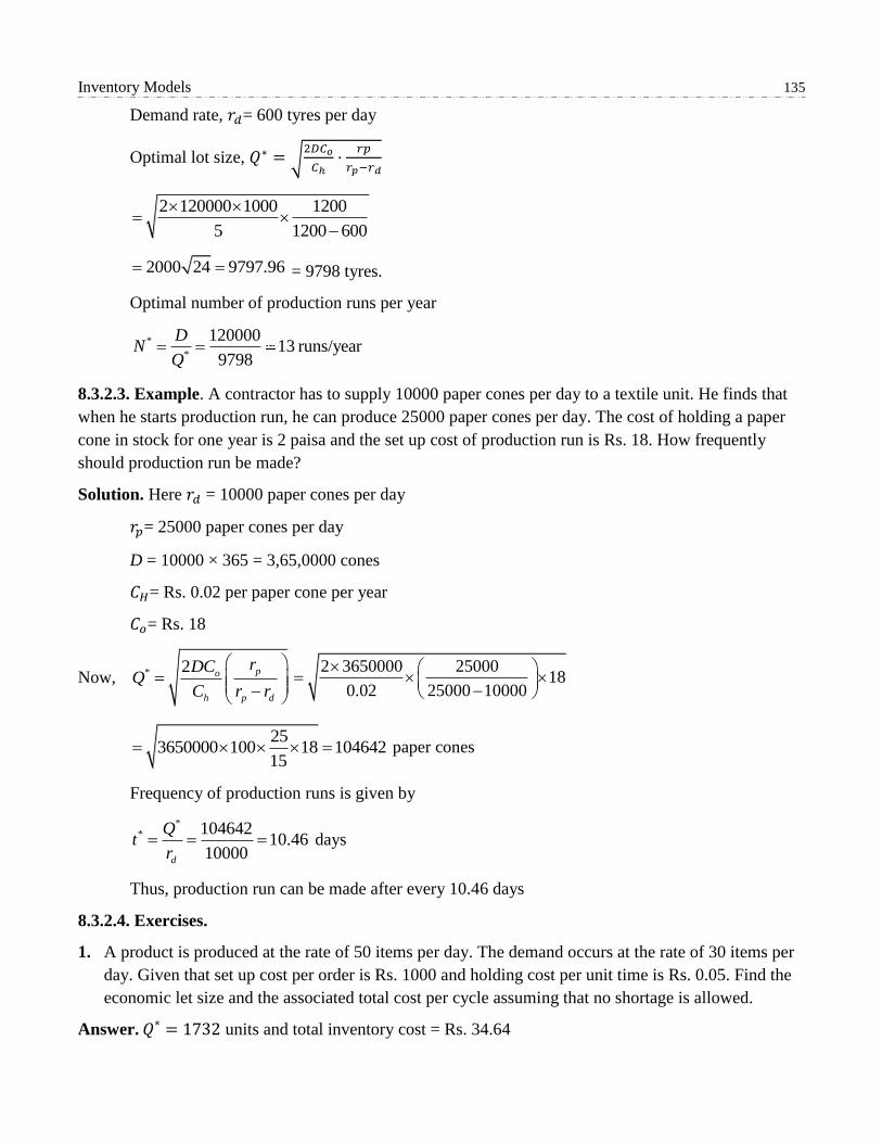
Inventory Models 135
Demand rate, 𝑟𝑑= 600 tyres per day
Optimal lot size, 𝑄∗ = √2𝐷𝐶𝑜
𝐶ℎ⋅
𝑟𝑝
𝑟𝑝−𝑟𝑑
2 120000 1000 1200
5 1200 600
2000 24 9797.96 = 9798 tyres.
Optimal number of production runs per year
*
*
12000013 runs/year
9798
DN
Q
8.3.2.3. Example. A contractor has to supply 10000 paper cones per day to a textile unit. He finds that
when he starts production run, he can produce 25000 paper cones per day. The cost of holding a paper
cone in stock for one year is 2 paisa and the set up cost of production run is Rs. 18. How frequently
should production run be made?
Solution. Here 𝑟𝑑 = 10000 paper cones per day
𝑟𝑝= 25000 paper cones per day
D = 10000 × 365 = 3,65,0000 cones
𝐶𝐻= Rs. 0.02 per paper cone per year
𝐶𝑜= Rs. 18
Now, * 2 po
h p d
rDCQ
C r r
2 3650000 2500018
0.02 25000 10000
25
3650000 100 18 10464215
paper cones
Frequency of production runs is given by
*
* 10464210.46
10000d
Qt
r days
Thus, production run can be made after every 10.46 days
8.3.2.4. Exercises.
1. A product is produced at the rate of 50 items per day. The demand occurs at the rate of 30 items per
day. Given that set up cost per order is Rs. 1000 and holding cost per unit time is Rs. 0.05. Find the
economic let size and the associated total cost per cycle assuming that no shortage is allowed.
Answer. 𝑄∗ = 1732 units and total inventory cost = Rs. 34.64

136 Operations Research Techniques
2. The annual demand for a product is 100000 units. The rate of production is 200000 units per year.
The set up cost per production run is Rs. 500 and the variable production cost of each item is Rs. 10.
The annual holding cost per unit is 20% of its value. Find the optimum production lot size and the
length of the production run.
Answer. 𝑄∗ = 10000 units, 𝑡1∗ =
10000
200000= 0.05years
3. An item is produced at the rate of 50 items per day. The demand occurs at the rate of 25 items per
day. If the set-up cost is Rs. 100 per set up and holding cost is Re 0.01 per unit of item per day, find
the economic lot size for one run, assuming that shortages are not allowed. Also find the time of
cycle, length of each production run, minimum total cost per day and maximum inventory level.
Answer. 𝑄∗ = 1000 items, Cycle time, 𝑡𝑙∗= 40 days
Length of each production run, 𝑡1∗= 20 days, Maximum inventory level = 500 items
Minimum daily cost = Rs. 5
4. A company uses 100000 units of a particular item per year. Each item costs Rs. 2. The production
engineering department estimates set up cost at Rs. 25 and the accounting department estimates the
holding cost as 12.5% of the value of the inventory per day.
Replenishment rate is uniform 500 units per day.
Assuming 250 working days (per replenishment purpose), calculate
(a) Optimal setup quantity
(b) Total cost on the basis of optimal policy
(c) Optimal number of set up
Answer. (a) 𝑄∗= 10000 units
(b) Total minimum cost = * 200000 200500TC
(c) Optimum number of set ups =𝐷
𝑄∗= 10
8.3.3. Model III: Economic Order Quantity with Different Rates of Demands in Different Cycles
Here the stock will vanish at different time periods with a policy of ordering same quantity for
replenishment of inventory.
Here replenishment rate is infinite, replenishment is instantaneous and shortage is not allowed.
The total demand D is specified as demand during total time period T and stock level Q is fixed.
Number of production cycles, 𝑛 =𝐷
Q
Let the demand in different time periods be 𝐷1, 𝐷2, … , 𝐷𝑛 respectively so that total demand in time T is
1 2 nD D D D

Inventory Models 137
Where, 𝑇 = 𝑡1 + 𝑡2 + ⋯ + 𝑡𝑛
Cost of ordering in time T is given by𝐷
𝑄𝐶𝑜
Let 𝐶ℎ be the holding cost per item per unit time
Then carrying cost for time T is
1 2
2 2
nh h h
QtQt QtC C C
r
1 22 2
h n h
Q QC t t t C T
Total inventory cost, 𝑇𝐶 =𝐷𝐶𝑜
𝑄+
𝑄
2𝐶ℎ𝑇
Total cost is minimum, when 𝐷𝐶𝑜
𝑄=
𝑄
2𝐶ℎ𝑇
i.e.
2 2o o
h h
DC C DQ
C T C T
* 2 o
h
C DQ
C T
This result is similar to the result of Model I with the only different that uniform demand is replaced by
average demand.
Here, *
0
2h
DTC C C
T
and total minimum cost 0
2h
DC C
T + cost of material
Remark: If T = 1 year, then results of this model are exactly same as that of model I.
8.3.4. Model IV: Economic Order Quantity when Shortages are Allowed
The assumptions of this model are same as that of model I except that shortages are allowed and
shortages may occur regularly. Let sC be the shortage cost per unit of time per unit quantity.
Ordering cost o
DC
Q
Total inventory over the time period, 1
1
2t Mt
Average inventory at any time 1
1/
2Mt t
Inventory holding cost 1
2h
MtC
t

138 Operations Research Techniques
Total amount of shortage over time period 2
1
2t St
Average shortage at any time 21
2
St
t
Shortage cost 2
2
1
2s
StC
t
From (1),
2 2 2 2
02 2 2 2 0h sDC M C C Q QM Q QM M
i.e., 2 2 2 0s h s oC Q M C C DC
i.e.,
2 2
2
22s
s h s o
h s
Q CC Q C C DC
C C
[using (3)]
i.e. 2 2
2 2ss o
h s
Q CC Q DC
C C
i.e. 2 2
2 2s h s so
h s
C C C CQ DC
C C
i.e. 2
3
3
2 oh
h
DCQ C C
C C
* 2 o h s
h s
DC C CQ
C C
and * 02 s
h h s
DC CM
C C C
Total minimum cost
* **2
0* * *2 2h s
Q MD MC C C
Q Q Q
2 so h
h s
CDC C
C C
Total cost, 1 21 1
2 2o h s
t tDTC C M C S C
Q t t
Using the relationship for similar triangles, we have
1t M
t Q and 2t S
t Q
1
Mt t
Q and 2
St t
Q
So
221
2 2o h s
Q MD MTC C C C
Q Q Q
since S = a – M

Inventory Models 139
Since TC is function of two variables Q and M, so in order to determine the optimal order size and
optimal shortage level, we put TCQ
and TC
M
, both equal to zero so that
22
2 2 2
2 10
2 2
o h sQ Q M Q MDC M C C
Q Q Q
(1)
and
2
1 02
sh
CMC Q M
Q Q (2)
From (2),
0h s sMC C Q MC
s
h s
CM Q
C C
(3)
8.3.4.1. Example. A contractor undertakes to supply Diesel engines to a truck manufacturer at a rate of
20 engines per day. The penalty in the contract is Rs. 100 per engine per day late for missing the scheduled
delivery date. The cost of holding an engine in stock for one month is Rs. 150. His production process is
such that each month (30 days) he starts producing a batch of engines through the shops and all these are
available for supply after the end of the month. Determine the maximum inventory level at the beginning
of each month.
Solution. Here, 150
Rs.30
hC per engine per day= Rs. 5 per engine per day
sC = Rs. 100 per engine per day
D = 20 engines per day
*t = 30 days
∴ Optimum inventory level at the beginning of each month
* * *,s s
h s h s
C CM Q Dt
C C C C
10020 30
5 100
= 571 engines
8.3.4.2. Example. A dealer supplies you the following information with regard to a product dealt in by
him.
Annual demand = 10,000 units
Ordering cost = Rs. 10 per order, Price = Rs. 20 per unit
Inventory carrying cost = 20% of the value of inventory per year
The dealer is considering the possibility of allowing some back order (stock ordered) to occur. He has
estimated that the annual cost of back ordering will be 25% of the value of inventory.
(i) What is the optimal number of units of product he should buy in one lot?
(ii) What quantity of product should be allowed to be back ordered, if any?

140 Operations Research Techniques
(iii) What would be maximum quantity of inventory at any time of the year?
(iv) Would you recommended to allow back-ordering? If so, what would be the annual cost saving
by adopting the policy of back ordering?
Sol. Here, D = 10,000 units
oC = Rs. 10 per order
hC = 20% of Rs. 20 = Rs. 4 per unit per year
sC = 25% of Rs. 20 = Rs. Per unit per year
(i) (a) When stock outs are not permitted:
* 2 2 10000 10
223.6 units4
o
h
DCQ
C
(b) When back ordering is permitted
* 2 o h s
h s
DC C CQ
C C
2 10000 10 4 5
90000 300 units4 5
(ii) Optimal quantity of the product to be back-ordered is given by
* * h
h s
CS Q
C C
4
300 133 units4 5
(iii) Maximum inventory level, * * * 300 133 167 unitsM Q S
(iv) Minimum total variable inventory cost in case shortages is not allowed
0223.6 2 hTC DC C
2 10000 10 4 = Rs. 894.43
Minimum total variable inventory cost in case shortage is allowed
= TC (300)
5
2 2 10,000 10 44 5
so h
h s
CDC C
C C
= Rs. 666.67

Inventory Models 141
Since TC (300) <TC (223.6), the dealer should accept the proposal for back ordering as this will result in
a saving of Rs. (894.43 – 666.67) = Rs. 22776 per year.
8.3.4.3. Exercise. A contractor undertakes to supply diesel engines to a truck manufacturer at a rate of 25
engines per day. He finds that the cost of holding a completed engine in stock is Rs. 16 per month and
there is a clause in the contract penalizing him Rs. 10 per engine per day late for missing the scheduled
delivery date production of engines is in batches and each time a new batch is started, there are setup costs
of Rs. 10,000. How frequently should batches be started and what should be the initial inventory level at
the time, each batch is completed?
Solution. * 2 o h s
h s
DC C CQ
C C
1610
2 25 10,000 3011 10
30
=994 units (app.)
*
* 99439.76
25
Qt
D ≃ 40 days
8.3.5. Problems of EOQ with Price Breaks
In the real world, it is not always true that the unit cost of an item is independent of the quantity procured.
Often discounts are offered for the purchase of large quantities. These discounts take the form of price
breaks.
Let us consider a manufacturer, who is encountered with a problem of determining an optimum production
quantity for each production run and an optimal interval between successive runs. The following
conditions are assumed to hold
(i) Demand is known and uniform
(ii) Shortages are not allowed
(iii) Production for supply commodities is instantaneous
Let Q be the lot size in each production run, D, total number of units produced or supplied over
the time period, 0C the cost per production run, R cost of manufacturing (or purchasing) per unit and I
inventory carrying charge expressed as a % of the value of the average inventory. Then total cost is given
by
TC = Purchase cost + Holding cost + Ordering cost
1
2o
DDk QkI C
Q
*
1
2
od TC DC
kIdQ Q
2
0
2 3
2DCdTC
dQ Q
For maxima or minima, 0d
TCdQ

142 Operations Research Techniques
i.e., 0
2
10
2
DCkI
Q
i.e., 2 oDC
QkI
At 2
2
2, 0o
d TCDCQ
kI dQ
Hence total cost is minimum when 2 oDC
QkI
So total minimum cost, * *
*
1
2o
DTC Q Dk Q kI C
Q
21
2 2
o o
o
DC DC kIDk kI
kI DC
2 oDk DC kI
8.3.5.1. Purchase Inventory Model with One Price Break
The purchase inventory model with only one price break may be represented as follows:
Range of quantity Purchase cost (per unit)
0 ≤ Q<b 1P
b ≤ Q 2P
Where b is the quantity at and beyond which the quantity discount applies and 2 1P P
The procedure for obtaining EOQ may be summarized in the following steps:
Step 1. Calculate optimum order quantity *
2Q for the lowest price (highest discount) i.e.
2
2
2o oDCQ
P I
and compare it with the quantity b
If 2
oQ b , calculate optimum order quantity 1
oQ for price 1P and compare total inventory cost for 1
oQ Q
with Q = b which given by
11 1 1
1 2
oo
oo
QDTC Q DP C IP
Q
2 22
o
D bTC b DP C IP
b
If 1
oTC Q TC b , then oQ b otherwise
1
o oQ Q .
8.3.5.1.1. Example. Find the optimum order quantity for a product for which the price breaks are as
follows:

Inventory Models 143
Quantity Unit cost (Rs.)
0 ≤ Q< 500 10.00
500 ≤ Q 9.25
The monthly demand for the product is 200 units, the cost of storage is 2% of the unit cost and ordering
cost is Rs. 350.
Solution. We are given
oC = Rs. 350
D = 200 units per month
I = 2% = 0.02
1P = Rs. 10
2P = Rs. 9.25
Highest discount available is Rs. 9.25. So we compute 2
oQ as
2
2
2 2 200 350
0.02 9.25
o oDCQ
IP
= 870 units
Since 2 500oQ b , the optimum purchase quantity is given by
2
o oQ Q = 870 units.
8.3.5.1.2. Example. Find the optimal order quantity for a product having the following characteristics:
Annual demand = 2400 units
Ordering cost = Rs. 100
Cost of storage = 24% of the unit cost
Price break
Quantity Unit cost (Rs.)
0 ≤ Q< 500 10
500 ≤ Q 9
Solution. We have D = 2400 units per year
I = 0.24
oC = Rs. 100
1P = Rs. 10
2P = Rs. 9
Highest discount available is Rs. 9, so we compute *
2Q as
*
2
2 2 2400 100
9 0.24
os
DCQ
P I
= 471 units
Since *
2 500Q , *
2Q is not feasible
144 Operations Research Techniques
We calculate *
1Q as
*
1
1
2 2 2400 100
10 0.24
oDCQ
PI
= 447 units.
Now total cost corresponding to order size 447 is
*
* 11 1 1*
1 2o
QDTC Q DP C IP
Q
2400 100 447
2400 10 0.24 10447 2
= 2400 + 536.91 + 536.4 = Rs. 25073.31
Total cost at price break is
TC (b) = TC (500)
2 2
2o
D bDP C IP
b
2400 500
2400 9 100 0.24 9500 2
= Rs. 22620
Since *
1TC b TC Q , the optimal order quantity is the price discount quantity is 500 units.
8.3.5.2. EOQ Problems with Two Price Breaks
When there are two price breaks i.e. two quantity discounts, the situation can be represented as
Range of quantity Purchase cost per unit
0 ≤ Q<b1 P1
b1 ≤ Q<b2 P2
b2 ≤ Q P3
where 1b and 2b are the quantities which determine this price discount. The procedure for obtaining EOQ
may be summarized in the following steps:
1. Compute the optimal order quantity for the lowest price. Let it be *
3Q .
2. If *
3 2Q b , the optimum order quantity is *
3Q .
3. If *
3 2Q b , calculate *
2Q , the optimal order quantity for the next lowest price.
4. If *
1 2 2b Q b , then compare *
2TC Q and 2TC b to determine the optimum purchase quantity.
5. If *
2 1Q b , calculate *
1Q and compare 1TC b , 2TC b and *TC Q to determine the optimum,
purchase quantity.

Inventory Models 145
8.3.5.2.1. Example. Find the optimal order quantity for a product for which the price discounts are as:
Range of quantity Unit price (Rs.)
0 500Q 10.00
500 750Q 9.25
750 Q 8.75
The monthly demand for the product is 200 units, storage cost is 2% of unit cost and ordering cost is Rs.
100.
Solution. Here D = 200 units
I = 2% of unit cost
0C = Rs. 100 per order
1P = Rs. 10
2P = Rs. 9.25
3P = Rs. 8.75
We calculate *
3Q as
*
3
3
2 2 200 100
8.75 0.02
oDCQ
IP
= 475 units
Since * *
3 2 3750,Q b Q is not feasible.
Now *
2
2
2 2 200 100
0.02 9.25
oDCQ
IP
= 465 units
Since *
2 1 500Q b , we compute *
1Q
*
1
1
2 2 200 100
0.02 10
oDCQ
IP
= 447 units.
Now,
*
* 1 11 1 *
1 2o
Q IPDTC Q DP C
Q
200 447
200 10 100 0.02 10447 2
= 2000 + 44.74 + 44.70 = Rs. 2089.44
1 500TC b TC
12 2
1 2o
bDDP C IP
b
200 500
200 9.25 100 0.02 9.25500 2
1850 40 46.25 = Rs. 1936.25
2 750TC b TC

146 Operations Research Techniques
23 3
2 2o
bDDP C IP
b
200 750
200 8.75 100 0.02 8.15750 2
= 1750 + 26.67 + 65.62 = Rs. 1842.29
The lowest total inventory cost is Rs. 1842.24
So optimal order quantity is *
2 750Q b
8.3.5.3. Purchase Inventory Model with n Price Breaks
When there are n price breaks, the situation may be illustrated as
Range of quantity Purchase cost per unit
10 Q b 1P
1 2b Q b 2P
1nb Q nP
where 1 2 1, , nb b b are the quantities which determine the price breaks. Let * * *
1 2, , , nQ Q Q be EOQ
corresponding to prices 1 2, , , nP P P respectively. The procedure for obtaining optimum order quantity
is:
1. Compute *
nQ . If *
1n nQ b , then the optimum purchase quantity is *
nQ .
2. If *
1,n nQ b then compute *
1nQ .
If *
1 2n nQ b , then optimum order quantity is determined by comparing *
1nTC Q with 1nTC b .
3. If *
1 2n nQ b , compute *
2nQ . If *
2 3n nQ b , then optimum order quantity is determined by
comparing *
2nTC Q with 2nTC b and 1nTC b .
4. If *
2 3n nQ b , compute *
3nQ
If *
3 4n nQ b , then optimum order quantity is determined by comparing *
3nTC Q with 3nTC b ,
2nTC b and 1nTC b .
5. Continue in this way until *
1; 0 1;n j n j
Q b j n and then compare *
n jTC Q with n jTC b
, 1 2 1, , ,n j n j nTC b TC b TC b .
This procedure involves a finite number of steps.
8.3.5.3.1. Example. The annual demand for a product is 500 units. The cost of storage per unit per
year is 10% of the unit cost. The ordering cost is Rs. 180 for each order. The unit cost depends upon the
amount ordered. The range of amount ordered and the unit cost price are as follows:

Inventory Models 147
Range of amount ordered Price per unit
0 500Q Rs. 25
500 1500Q Rs. 24.80
1500 3000Q Rs. 24.60
3000 Q Rs. 24.40
Find the optimal order quantity.
Solution. Here D = 500 units
oC = Rs. 180 per order
I = 0.10
1b = 500, 2b = 1500, 3b = 3000
1P = Rs. 25, 2P = Rs. 24.80
3P = Rs. 24.60, 4P = Rs. 24.40
Step 1 *
4
4
2 2 500 180 1000 10 18000
0.10 24.40 2440
oDCQ
IP
180
1000 271.62440
≃ 272 units
Since *
4 3Q b , we compute *
3Q .
Step 2 *
3
3
2 2 500 180
0.16 24.60
oDCQ
IP
18
100 270 units246
Since *
3 2Q b , we compute *
2Q
Step 3 *
2
2
2 2 500 180
0.10 24.80
oDCQ
IP
= 269 units
Since *
2 1Q b , we compute *
1Q
Step 4 *
1
2 500 180 18010000 72000
0.10 25 25Q
= 268 units.
Now we compute *
1 1 2 3, , ,TC Q TC b TC b TC b and compare them to get optimal order quantity.
* *
1 1 1 1*
1
1
2o
DTC Q DP C Q IP
Q
500 268
500 25 180 0.10 25268 2
= 12500 + 335.82 + 335 = Rs. 13170.82

148 Operations Research Techniques
1 2 1 2
1
1
2o
DTC b DP C b IP
b
500 500
500 24.80 180 0.10 24.80500 2
= 12400 + 1800 + 620 = Rs. 14820
2 3 2 3
2
1
2o
DTC b DP C b IP
b
500 1
500 24.60 180 1500 0.10 24.601500 2
= 12300 + 60 + 1845 = Rs. 14205
3 4 3 4
3
1
2o
DTC b DP C b IP
b
500 1
500 24.40 180 3000 0.10 24403000 2
= 12200 + 30 + 3660 = Rs. 15890
Since *
1 2 1 3TC Q TC b TC b TC b ,
Optimum order quantity is *
1Q i.e. 268 units.
8.4. CHECK YOUR PROGRESS
1. Why inventory is maintained?
2. Explain the meaning of inventory control.
3. Explain the inventory model when demand rate is uniform.
4. Derive EOQ model for an inventory problem when shortages are allowed.
8.5. SUMMARY
Inventory may be defined as stock of idle resources that are stored or reserved in order to ensure smooth
and efficient running of business affairs as inventories are essential for almost all business. In this
chapter, we explained the concept of inventory control and EOQ. The models discussed in this chapter
are:
(i) EOQ Model with Uniform Demand,
(ii) EOQ Model with uniform replenishment,
(iii) EOQ with different rates of demands in different cycles,
(iv) EOQ Model when shortages are allowed, and
(v) EOQ Model with price breaks

9 GAME THEORY
Structure
9.1. Introduction
9.2. Some Basic Definitions
9.3. Two-Person Zero-Sum Game
9.4. Pure Strategies: Game with Saddle Points
9.5. The Rule of Dominance
9.6. Mixed Strategies: Game without Saddle Points
Algebraic Method
Graphical Method
Linear Programming Method
9.7. Check Your Progress
9.8. Summary

150 Operations Research Techniques
9.1. INTRODUCTION
In real-life, we can see a great variety of competitive situations. Game theory provides tools for analysing
situations in which parties, called players, make decisions that are interdependent. This interdependence
causes each player to consider the other player’s possible decisions, or strategies, in formulating strategy.
A solution to a game describes the optimal decisions of the players, who may have similar, opposed, or
mixed interests, and the outcomes that may result from these decisions. So, one can say that it is a type of
decision theory. Game theory was originally developed by John von Neumann (called the father of game
theory) and his colleague Oskar Morgenstern to solve problems in economics.
In this chapter, first we define some basic terms used in game theory then we shall discuss two-person
zero-sum-games (also known as rectangular games), games with saddle point in which we study minimax
and maximin criterion. Also, we shall explain rules of dominance which are used to reduce the size of the
payoff matrix and discuss solution methods for game without saddle point namely algebraic method,
graphical method and linear programming method.
9.1.1. Objectives. The objective of these contents is to get familiar reader with game theory. After
studying this chapter, reader should be able to describe the following concepts like:
Minimax and Maximin Principle
Pure Strategies: Game with Saddle Points
The Rule of Dominance
Mixed Strategies: Game without Saddle Points
9.2. SOME BASIC DEFINITIONS
Game: A competitive situation is called a game if it has the following properties
a) There are finite numbers of participants called players.
b) Each player has finite number of strategies available to him.
c) Every game result in an outcome.
Player: Each participant of a game is called a player.
Number of players: If a game involves any two payers, it is called a two-person game. However, if the
number of players is more than two, the game is known as n-person game.
Payoff: A quantitative measure of satisfaction, a person gets at the end of each play, is called a payoff.
Play: A play is said to occur when each player chooses one of his activities.
Strategy: The strategy for a payer is the list of al possible actions or moves available to him. Generally,
two types of strategies are employed by players in a game.
(i) Pure strategy: It is a decision rule which is always used by the player to select any one particular
course of action. The objective of the payer is to maximize gains or minimize losses.
(ii) Mixed strategy: When the players use a combination of strategies and each player always keep
guessing as to which course of action is to be selected by the other on a particular occasion, then this is
known as mixed strategy. Thus, the mixed strategy is a selection among pure strategies with fixed
probabilities.

Game Theory 151
Zero-sum game. A game in which the algebraic sum of the outcomes for all the participants equals zero
for very possible combination of strategies, is called a zero-sum game.
A game which is not zero-sum is called a non-zero-sum game.
Optimal strategy. A course of action or play which puts the player in the most preferred position,
irrespective of the strategy of his competitors, is called optimal strategy.
Value of the game. The expected payoff when the players follow their optimal strategy is called the value
of the game.
9.3. TWO-PERSON ZERO-SUM GAME
A game with only two-persons is said to be two-person zero-sum game if the gain of one player is equal
to the loss of the other so that total sum is zero.
9.3.1. Payoff Matrix: In a two-person game, the payoffs in terms of gains or losses, when players select
their particular strategies can be represented in the form of a matrix, called the payoff matrix of the player.
If the game is zero-sum, the gain of one player is equal to the loss of the other and vice-versa. So, one
player’s payoff table would contain the same amounts I payoff table of the other payer with the sign
changed. If the player A has strategies A1, A2, …, An and the player B has strategies B1, B2, …, Bn and if
ija represent the payoffs that the player A gains from player B when player A chooses strategy i, and player
B chooses strategy j then payoff matrix for player A is given by
Player B’s strategies
Player A’s strategies
9.3.2. Basic Assumptions of the Game:
Rules of the game are given as follows:
Each player has available to him a finite number of possible courses of action. The list may not be the
same for each player.
Players act rationally and intelligently.
The decisions of both the payers are made individually, prior to the play, with no communication
between them.
One player attempts to maximize gains and the other attempts to minimize losses.
The players simultaneously select their respective courses of action.
The payoff is fixed and determined in advance.
List of strategies of each player and the amount of gain or loss on an individual’s choice of strategy is
known to each player in advance.

152 Operations Research Techniques
9.4. PURE STRATEGIES: GAMES WITH SADDLE POINT
Consider the payoff matrix of a game which represents payoff of player A. Now, the objective of the study
is to know how these players must select their respective strategies so that they may optimize their payoff.
Such a decision-making criterion is referred to as the minimax-maximin principle.
For payer A, the minimum value in each row represents the least gain to him if he chooses his particular
strategy. He will then select the strategy that gives the largest gain among the row minimum values. This
choice of player A is called the maximin principle and the corresponding gain is called the maximin value
of the game denoted by v.
For player B, who is assumed to be loser, the maximum value in each column represents the maximum
loss to value in each column represents the maximum loss to him if he chooses his particular strategy. He
will then select the strategy that gives minimum loss among the column maximum values. This choice of
player B is called the minimax principle and the corresponding loss is called the minimax value of the
game, denoted by v .
Saddle point. A saddle point of a payoff matrix is that position in the payoff matrix where maximum of
row minima coincides with the minimum of the column maxima. The saddle point need not be unique.
Value of the game. The amount of payoff at the saddle point is called the value of the game, denoted by v.
Fair game. A game is said to be fair if 0v v .
Strictly determinable game. A game is said to be strictly determinable if v v v .
9.4.1. Procedure to Determine Saddle Point
a) Select the minimum element in each row and enclose it in a rectangle box.
b) Select the maximum element in each column and enclose it in a circle.
c) Find the element which is enclosed by the rectangle as well as the circle such element is the
value of the game and that position is a saddle point.
9.4.2. Example. For the game with payoff matrix:
Determine the optimal strategies for players A and B.
Also determine the value of game.
Is this game (i) fair? (ii) strictly determinable?
Solution. Select the row minimum and enclose it in a rectangle. Then select the column maximum and
enclose it in a circle.

Game Theory 153
Saddle point is 1 3,A B .
Value of game = –2
Optimal strategy for A is A1 and for B is B3.
The game is strictly determinable. Since value of game is not zero, the game is not fair.
9.4.3. Example. Determine which of the following two-person zero-sum games are strictly determinable
and fair. Give optimum strategies for each player in case of strictly determinable games:
Solution. (a) Payoff matrix for player A is:
maximin value 0v
minmax value 0v
Since 1, 1v v , game is not strictly determinable.
9.4.4. Example. Solve the game hide payoff matrix is given by
Solution. Select the row minimum and enclose it in a rectangle select the column maximum and enclose
it in a circle.
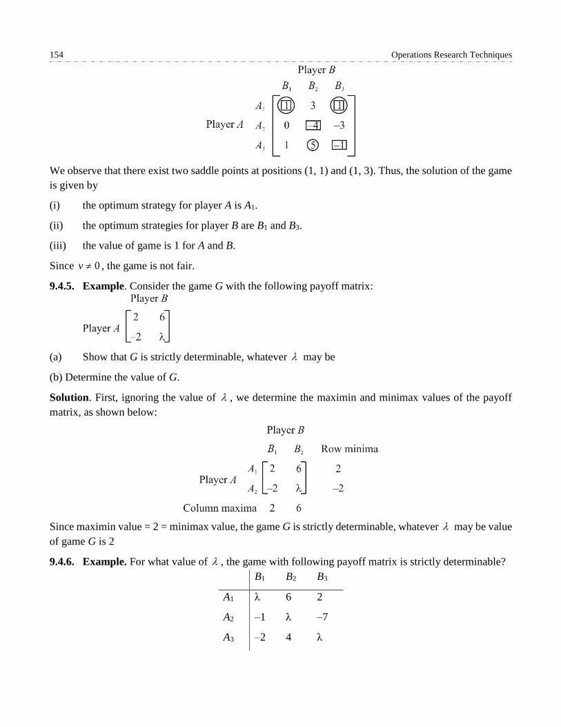
154 Operations Research Techniques
We observe that there exist two saddle points at positions (1, 1) and (1, 3). Thus, the solution of the game
is given by
(i) the optimum strategy for player A is A1.
(ii) the optimum strategies for player B are B1 and B3.
(iii) the value of game is 1 for A and B.
Since 0v , the game is not fair.
9.4.5. Example. Consider the game G with the following payoff matrix:
(a) Show that G is strictly determinable, whatever may be
(b) Determine the value of G.
Solution. First, ignoring the value of , we determine the maximin and minimax values of the payoff
matrix, as shown below:
Since maximin value = 2 = minimax value, the game G is strictly determinable, whatever may be value
of game G is 2
9.4.6. Example. For what value of , the game with following payoff matrix is strictly determinable?
B1 B2 B3
A1 λ 6 2
A2 –1 λ –7
A3 –2 4 λ

Game Theory 155
Solution. Ignoring the value of , we determine the maximin and minimax values of the payoff matrix,
as shown below
Here maximin value = 2, minimax value = –1.
The value of game lies between –1 and 2.
For strictly determinable game, since maximin value equals minimax value, we must have 1 2 .
9.4.7. Exercises. Solve the games whose payoff matrices are given below.
1.
Answer. v = 1
2.
Answer. 2 2, , 5A B v
3.
Answer. 1 1 1 3, , , , 1A B A B v for A.
4.
Answer. 1 1 1 2, , , , 6A B A B v

156 Operations Research Techniques
5.
Answer. (II, III), 4v
6 Determine which of the following two-person zero-sum games are strictly determinable and fair?
Give the optimum strategies for each player in case of strictly determinable games.
Answer. (a) 1 1, , 5A B v , not fair (b) 1 2,A B , value = 6, not fair.
9.5. PRINCIPLE OF DOMINANCE
The principle of dominance is used to reduce the size of a games payoff matrix by eliminating a course of
action which is so inferior to another as never to be used. Such a course of action is said to be dominated
by the other. It is applicable to both pure and mixed strategy problems. However, this rule is especially
useful for the evaluation of two-person zero-sum games where a saddle point does not exist.
In general, the following rules of dominance are used to reduce the size of payoff matrix.
Rule 1. If all the elements in a column are greater than or equal to the corresponding elements in another
column, then that column is dominated and can be deleted from the matrix.
Rule 2. If all the elements in a row are less than or equal to the corresponding elements in another row,
then that row is dominated and can be deleted from the matrix.
Rule 3. If all the elements in a column are greater than or equal to the average of the corresponding
elements of two or more other columns, then that column can be deleted.
Rule 4. If all the elements in a row are less than or equal to the average of the corresponding elements of
two or more other rows, then it can be deleted.
9.5.1. Example. Reduce the following game to 2 × 2 game using principle of dominance.
Player A
Player B
I II III IV V VI
I 4 2 0 2 1 1
II 4 3 1 3 2 2
III 4 3 7 –5 1 2
IV 4 3 4 –1 2 2
V 4 3 3 –2 2 2

Game Theory 157
Solution. Column I, II and IV are dominated by column V, so columns I, II and VI are deleted. The
reduced matrix is
Now row I is dominated by row 2 and row 5 is dominated by row 4. Hence deleting rows I and V, we
have
Now none of single row (or column) dominates another row (or column. However, column V is dominated
by the average of columns III and IV. Hence deleting column V, we have
Now average of row II and row III gives the row (4, –1) which dominates the row IV. Hence deleting row
IV, we have
9.5.2. Example. Reduce the following game into 2 × 2 game using the rules of dominance.

158 Operations Research Techniques
Solution. First, we delete the column 3 as all the elements of this column are greater than that of first
column after that we delete 3rd row as all the elements of row 3 are less than the corresponding elements
of row 2. Hence the reduced matrix is
9.6. MIXED STRATEGIES: GAMES WITHOUT SADDLE POINT
Pure strategies are available as optimal strategies only for those games which have a saddle point. For
games which do not have a saddle point can be solved by applying the concept of mixed strategies. Her,
we study algebraic, graphical and linear programming method to solve mixed strategies games.
9.6.1. Algebraic Method
Consider the two-person zero-sum game with the following payoff matrix:
If this game is to have no saddle point, the two largest elements of the matrix must constitute one of the
diagonals. We have assumed this and therefore both players use mixed strategies. Our task is to determine
the probabilities with which both players choose their course of action.
In this game, let player A play the strategies 1A and 2A with respective probabilities p and 1 – p
and let player B play his strategies B1 and B2 with respective probabilities q and 1 – q. The expected
payoffs to player A when B plays any one of his strategies B1 or B2 throughout the game, are given by
B’s Strategy A’s Strategy
1B 11 21 1a p a p
2B 12 22 1a p a p
Now in order that player A is unaffected with whatever choice of strategies B makes, we must have
11 21 12 221 1a p a p a p a p
11 12 22 21 22 21a a p a a p a a
22 21
11 12 22 21
a ap
a a a a

Game Theory 159
and
11 12
11 12 22 21
1a a
pa a a a
similarly, by equating the expected payoffs of the player B, for whatever choice of strategies player A
makes, we have
11 12 21 221 1a q a q a q a q
This implies
11 22 22 12 22 12a a a a q a a
So
22 12
11 21 22 12
a aq
a a a a
and
11 21
11 21 22 12
1a a
qa a a a
The value of game, v is found by substituting the value of p in one of the expressions for the expected
gains of A so that
11 21 1v a p a p
11 22 21 21 11 12
11 12 22 21 11 12 22 21
a a a a a a
a a a a a a a a
11 22 12 21
11 12 22 21
a a a a
a a a a
Hence the solution of the game is
A plays ,1p p where
22 21
11 12 22 21
a ap
a a a a
B plays ,1q q where
22 12
11 12 22 21
a aq
a a a a
and value of game,
11 22 12 21
11 21 22 12
a a a av
a a a a
.
9.6.1.1. Example. Solve the following game:
Solution. Here maximin value = 10 and minimax value = 15.
So, game has no saddle point.
Let the player A play his first strategy A1 with probability p, then he would play his second strategy A2
with probability 1 p . Then expected gain of A is B selects B1, is equal to 25 10 1p p i.e. 10 + 15
p and the expected gain of A if B selects strategy B2, is equal to 5 15 1p p i.e. 15 – 10 p.

160 Operations Research Techniques
Now in order that the player A may be unaffected with whatever choice B makes, the optimal plan for the
player A should be such that the expected payoffs for each of B’s strategies should be equal is
10 + 15 p = 15 – 10 p
5 1
25 5p and
1 41 1
5 5p
Hence, the player A would play his first strategy A1 with probability 1
5 and second strategy A2 with
probability 4
5.
Similarly, if the player B selects strategies B1 and B2 with probabilities q and 1 – q respectively, then the
expected loss to B when A adopts the strategy A1, is 25 q + 5(1 – q) and the expected loss to B when the
player A adopts the strategy A2, is 10 q + 15 (1 – q). By equating the expected losses of player B, for
whatever choice of strategies player A makes, we have
25 5 1 10 15 1q q q q
20 5 15 5q q
10 2
25 5q and
31
5q
Hence the player B would play his strategies B1 and B2 with probabilities 2
5 and
3
5 respectively.
Value of the game = expected payoff to player A
25 10 1p p
1 4
25 105 5
= 13.
9.6.1.2. Example. For the following game:
Determine the optimal strategies for each firm and value of the game.
Solution. Since maximin value = 10 and minimax value = 15, there is no saddle point.
We apply rules of dominance to reduce the size of payoff matrix. Since each element of second row is less
than the corresponding elements of first row, second row is dominated by first row. So, deleting the second
row, the reduced matrix becomes

Game Theory 161
In the reduced matrix, each element of second column is more than the corresponding elements in first
column, so second column is dominated by first column. Thus after deleting the second column, the
reduced matrix becomes
Further second row is dominated by third row, so we delete second row to get reduced matrix as
Now column one is dominated by column two. So, we delete column one and reduced matrix becomes
Now we solve the game by algebraic method in the same manner as we did in example 9.6.1.1. Thus, firm
A would select strategy A1 with probability 1
5 and strategy A4 with probability
4
5 and firm B would select
strategy B3 with probability 2
5 and strategy B4 with probability
3
5 and Value of game =
1 4
25 10 1 25 10 5 8 135 5
p p .
9.6.1.3. Example. In a game of matching coins with two players, suppose one player wins Rs. 2 when
there are two heads and wins nothing when there are two tails, and losses Re. 1 when there are one head
and one tail. Determine the payoff matrix, the best strategies for each player and the value of the game.
Solution. Let the two players be A and B. Then the payoff matrix for player A is

162 Operations Research Techniques
Here maximin value 1v ; minimax value 2v .
Since v v , given game has no saddle point. Let the player A plays H with probability p and T with
probability 1 – p. Then A’s expected gains when B plays H and T respectively, are 2 1 1p p and
0 1p p .
For best strategy of A, we have
2 1 1p p p .
so that 1 3
and14 4
p p . Therefore, best strategy for player A is to play H and T with probabilities
1 3and
4 4 respectively.
For player B, let the probability of the choice of H be q and that of T be 1 – q. For best strategy of
B, we have
2 1 1 1 0 1q q q q so that 1 3
and14 4
q q .
Hence player B should play H and T with probabilities 1 3
and4 4
respectively.
Value of game = 1
2 1 14
p p for player A.
9.6.1.4 Exercises. Solve the following games without saddle points.
1.
Answer. 4 3
,7 7
for player A,2 5
,7 7
for player B and Value of game = 0.
2. In a game of matching coins with two players, suppose A wins one unit of value, when there are
two heads, wins nothing when there are two tails and loses 1
2 unit of value when there are one head and
one tail. Determine the payoff matrix, the best strategies for each player and the value of game to A.
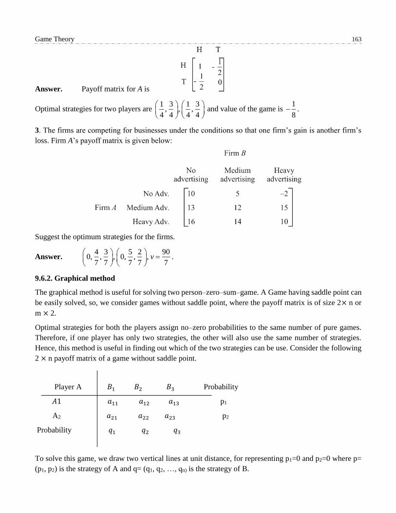
Game Theory 163
Answer. Payoff matrix for A is
Optimal strategies for two players are 1 3 1 3
, , ,4 4 4 4
and value of the game is 1
8 .
3. The firms are competing for businesses under the conditions so that one firm’s gain is another firm’s
loss. Firm A’s payoff matrix is given below:
Suggest the optimum strategies for the firms.
Answer. 4 3 5 2 90
0, , , 0, , ,7 7 7 7 7
v
.
9.6.2. Graphical method
The graphical method is useful for solving two person–zero–sum–game. A Game having saddle point can
be easily solved, so, we consider games without saddle point, where the payoff matrix is of size 2× n or
m × 2.
Optimal strategies for both the players assign no–zero probabilities to the same number of pure games.
Therefore, if one player has only two strategies, the other will also use the same number of strategies.
Hence, this method is useful in finding out which of the two strategies can be use. Consider the following
2 × n payoff matrix of a game without saddle point.
Player A 𝐵1 𝐵2 𝐵3 Probability
𝐴1 𝑎11 𝑎12 𝑎13 p1
A2 𝑎21 𝑎22 𝑎23 p2
Probability 𝑞1 𝑞2 𝑞3
To solve this game, we draw two vertical lines at unit distance, for representing p1=0 and p2=0 where p=
(p1, p2) is the strategy of A and q= (q1, q2, …, qn) is the strategy of B.

164 Operations Research Techniques
We now draw n line segments joining the points (0, a2j) and (1, a1j), j= 1, 2, …, n but excluding the end
points. The lower envelope of these lines gives the minimum expected gain of A as a function of p1. The
highest point o of this lower boundary of these lines will give maximum of the minimum gain of A, i.e.
maximin of A.
Now, the two strategies of player B corresponding to those lines which pass through the maximum point
can be determined. It helps in reducing the size of the game to (2 × 2), which can be easily solved by any
of the methods discussed earlier.
Remark: The (m×2) games are also treated in the same way except the upper boundary of the straight
lines corresponding to B’s expected payoff will give the maximum expected payoff to player B and the
lower point on this boundary will then give the minimum expected payoff (minimax value) and the
optimum value of probability 𝑞1 and 𝑞2.
9.6.2.1. Example. Use graphical method in solving the following game and find the value of the game
Solve the following game:
Player B
B1 B2 B3 B4
Player A 𝐴1 0 5 -2 3
𝐴2 2 3 4 1
Solution. Since maximin 𝑎𝑖𝑗 = 3 < 𝑚𝑖𝑛𝑖𝑚𝑎𝑥 𝑎𝑖𝑗 = 4, the game is to be solved by mixed strategies. We
therefore use the graphical method to reduce this to a 2× 2 by game as follows:
5 B2 5
4 4
3 B4 3
2 2
1 B1 1
0 0
-1 B3 -1
-2 -2
-3 -3
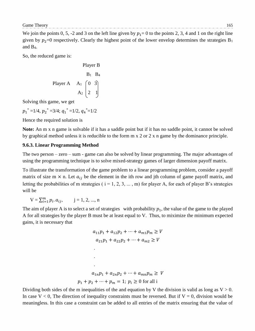
Game Theory 165
We join the points 0, 5, -2 and 3 on the left line given by 𝑝1= 0 to the points 2, 3, 4 and 1 on the right line
given by 𝑝2=0 respectively. Clearly the highest point of the lower envelop determines the strategies B1
and B4.
So, the reduced game is:
Player B
B1 B4
Player A A1 0 3
A2 2 1
Solving this game, we get
𝑝1* =1/4, 𝑝2
* =3/4; 𝑞1* =1/2, 𝑞4
*=1/2
Hence the required solution is
Note: An m x n game is solvable if it has a saddle point but if it has no saddle point, it cannot be solved
by graphical method unless it is reducible to the form m x 2 or 2 x n game by the dominance principle.
9.6.3. Linear Programming Method
The two person – zero – sum - game can also be solved by linear programming. The major advantages of
using the programming technique is to solve mixed-strategy games of larger dimension payoff matrix.
To illustrate the transformation of the game problem to a linear programming problem, consider a payoff
matrix of size m × n. Let 𝑎𝑖𝑗 be the element in the ith row and jth column of game payoff matrix, and
letting the probabilities of m strategies ( i = 1, 2, 3, ... , m) for player A, for each of player B’s strategies
will be
V = ∑ 𝑝𝑖. 𝑎𝑖𝑗𝑚𝑖=1 , j = 1, 2, ..., n
The aim of player A is to select a set of strategies with probability 𝑝1, the value of the game to the played
A for all strategies by the player B must be at least equal to V. Thus, to miximize the minimum expected
gains, it is necessary that
𝑎11𝑝1 + 𝑎12𝑝2 + ⋯ + 𝑎𝑚1𝑝𝑚 ≥ 𝑉
𝑎21𝑝1 + 𝑎22𝑝2 + ⋯ + 𝑎𝑚2 ≥ 𝑉
.
.
.
𝑎1𝑛𝑝1 + 𝑎2𝑛𝑝2 + ⋯ + 𝑎𝑚𝑛𝑝𝑚 ≥ 𝑉
𝑝1 + 𝑝2 + ⋯ + 𝑝𝑚 = 1; 𝑝𝑖 ≥ 0 for all i
Dividing both sides of the m inequalities of the and equation by V the division is valid as long as V > 0.
In case V < 0, The direction of inequality constraints must be reversed. But if V = 0, division would be
meaningless. In this case a constraint can be added to all entries of the matrix ensuring that the value of

166 Operations Research Techniques
the game (V) for the revised matrix becomes more than zero. After optimal solution is obtained for the
value of the game is obtained by subtracting the same constant value. Let 𝑝𝑖
𝑉⁄ = 𝑥𝑖 , (≥ 0). Then we get,
𝑎11
𝑃1
𝑉+ 𝑝21
𝑝2
𝑉+ ⋯ + 𝑎𝑚1
𝑝𝑚
𝑉≥ 1
𝑎12
𝑃1
𝑉+ 𝑝22
𝑝2
𝑉+ ⋯ + 𝑎𝑚2
𝑝𝑚
𝑉≥ 1
.
.
.
𝑎1𝑛
𝑃1
𝑉+ 𝑝2𝑛
𝑝2
𝑉+ ⋯ + 𝑎𝑚𝑛
𝑝𝑚
𝑉≥ 1
𝑝1
𝑉+
𝑝2
𝑉+ ⋯ +
𝑝𝑚
𝑉=1
Since, the objective of player A is to maximize the value of the game, V which is equivalent to minimize 1
𝑉 , the resulting linear programming problem can be stated as
𝑎11𝑥1 + 𝑎12𝑥2 + ⋯ + 𝑎𝑚1𝑥𝑚 ≥ 𝑉
𝑎21𝑥1 + 𝑎22𝑥2 + ⋯ + 𝑎𝑚2𝑥𝑚 ≥ 𝑉
.
.
.
𝑎1𝑛𝑥1 + 𝑎2𝑛𝑥2 + ⋯ + 𝑎𝑚𝑛𝑥𝑚 ≥ 𝑉
And 𝑥1, 𝑥2, … , 𝑥𝑚 ≥ 0, 𝑥𝑖 =𝑝𝑖
𝑉 ; i = 1, 2, ..., m
Similarly, Player B has a similar problem with the inequalities of the constraints reversed, i.e., minimize
the expected loss. Since minimizing of V is equivalent to maximizing 1
𝑉, therefore, the resulting
programming problem can be stated as:
Maximize 𝑍𝑞 (=1
𝑉) = 𝑦1 + 𝑦2 + ⋯ + 𝑦𝑛
Subjected to the constraints
𝑎11𝑦1 + 𝑎12𝑦2 + ⋯ + 𝑎1𝑛𝑦𝑛 ≤ 1
𝑎21𝑦1 + 𝑎22𝑦 + ⋯ + 𝑎2𝑛𝑦𝑛 ≤ 1 .
.
.
𝑎𝑚1𝑦1 + 𝑎𝑚2𝑦2 + ⋯ + 𝑎𝑚𝑛𝑦𝑛 ≤ 1
And 𝑦1, 𝑦2, … , 𝑦𝑛 ≥ 0
Where,𝑦𝑗 =𝑞𝑗
𝑉≥ 0 ; i = 1, 2, ..., n

Game Theory 167
It may be noted that the LP problem for the player B is the dual of LP problem for plater A and vice-
versa. Therefore, solution of the dual problem can be obtained from the primal simplex table. Since both
the players 𝑍𝑝 = 𝑍𝑞, the expected gain to player A in the game will be exactly equal to expected payoff
to player B.
Remark: Linear programming technique require all variables to be non-negative and therefore to derive
a non – negative value V of the game, the data to the problem, i.e., 𝑎𝑖𝑗 in the payoff table should be non –
negative. If there are some negative elements in the payoff table, a constant to every elements of the payoff
table must be added so as to make the smallest element zero; the solution to this new game give an optimal
mixed strategy for the new game. The value of the original game then equals to the value of the new game
minus the constant.
9.6.3.1. Example. For the following payoff matrix, transform the zero-sum game into an equivalent linear
programming problem and solve it by using simplex method.
Player B
Player A B1 B2 B3
A1
A2 A3
1 -1 3 3 5 -3 6 2 -2
Solution: The first step is to find out the saddle point (if any) in the payoff matrix as shown below
Player B
Player A B1 B2 B3 Row minimum
A1 1 -1 3 -1 ← Maximin
A2 3 5 -3 -3
A3 6 2 -2 -2
Column maximum 6 5 3 ← Minimax
The given game payoff matrix does not have a saddle point. Since, the maximin value is -1, therefore, it
is possible that the value of game (V) may be negative or zero because -1< 𝑉 < 1. Thus, a constant which
is at least equal to the negative of maximin value, i.e., more than -1 is added to all elements of the payoff
matrix. Thus, adding a constant number 4 to all the elements of the payoff matrix, the payoff matrix
becomes:
Player B
Player A B1 B2 B3 Probability
A1 5 3 7 𝑝1
A2 7 9 1 𝑝2
A3 10 6 2 𝑝3
Probability 𝑞1 𝑞2 𝑞3

168 Operations Research Techniques
Let 𝑝𝑖 (𝑖 = 1,2,3) and 𝑞𝑗 (𝑗 = 1,2,3) be the probabilities of selecting strategies
𝐴𝑖(𝑖 = 1,2,3) and 𝐵𝑗 (𝑗 = 1,2,3) by players A and B, respectively.
The expected gain for player A will be as follows:
5𝑝1 + 7𝑝2 + 10𝑝3 ≥ 𝑉 (if B uses strategy B1)
3𝑝1 + 9𝑝2 + 6𝑝3 ≥ 𝑉 (if B uses strategy B2)
7𝑝1 + 𝑝2 + 2𝑝3 ≥ 𝑉 (if B uses strategy B3)
𝑝1 + 𝑝2 + 𝑝3 = 1
and 𝑝1, 𝑝2, 𝑝3 ≥ 0
Dividing each inequality and equality by V, we get,
5𝑝1
𝑉+ 7
𝑝2
𝑉+ 10
𝑝3
𝑉≥ 1
3𝑝1
𝑉+ 9
𝑝2
𝑉+ 6
𝑝3
𝑉≥ 1
7𝑝1
𝑉+
𝑝2
𝑉+ 2
𝑝3
𝑉≥ 1
𝑝1
𝑉+
𝑝2
𝑉+
𝑝3
𝑉=
1
𝑉
In order to simplify, we define new variables:
𝑥1 = 𝑝1 𝑉⁄ , 𝑥2 = 𝑝2 𝑉⁄ 𝑎𝑛𝑑 𝑥3 = 𝑝3 𝑉⁄
The problem for player A, therefore becomes,
Minimize 𝑍𝑝 (=1/V) =𝑥1 + 𝑥2 + 𝑥3 subject to the constraints
5𝑥1 + 7𝑥2 + 10𝑥3 ≥ 1
3𝑥1 + 9𝑥2 + 6𝑥3 ≥ 1
7𝑥1 + 𝑥2 + 2𝑥3 ≥ 1
and 𝑥1, 𝑥2, 𝑥3 ≥ 0
player B’s objective is to minimize his expected losses which can be reduced to minimizing the value of
the game V. Hence, the problem of player B can be expressed as follows:
Minimize 𝑍𝑞 (=1/V) =𝑦1 + 𝑦2 + 𝑦3
subject to the constraints
5𝑦1 + 7𝑦2 + 10𝑦3 ≤ 1
3𝑦1 + 9𝑦2 + 6𝑦3 ≤ 1
7𝑦1 + 𝑦2 + 2𝑦3 ≤ 1
and 𝑦1, 𝑦2, 𝑦3 ≥ 0
where 𝑦1 = 𝑞1 𝑉⁄ , 𝑦2 = 𝑞2 𝑉⁄ 𝑎𝑛𝑑 𝑦3 = 𝑞3 𝑉⁄ .

Game Theory 169
It may be noted that problem of player A is the dual of the problem of player B. Therefore, solution of the
dual problem can be obtained from the optimal simplex table of primal.
To solve the problem of player B, introduce slack variables to convert the three inequalities to equalities.
The problem becomes
Minimize 𝑍𝑞 (=1/V) =𝑦1 + 𝑦2 + 𝑦3 + 0𝑠1 + 0𝑠2 + 0𝑠3
subject to the constraints
5𝑦1 + 7𝑦2 + 10𝑦3 + 𝑠1 = 1
3𝑦1 + 9𝑦2 + 6𝑦3 + 𝑠2 = 1
7𝑦1 + 𝑦2 + 2𝑦3 + 𝑠3 = 1 and 𝑦1, 𝑦2, 𝑦3, 𝑠1, 𝑠2, 𝑠3 ≥ 0
The initial solution is shown in Table 12.7.
Table 12.7 Initial Solution
Proceeding with usual simplex method, the optimal solution is shown in Table 12.8.
Table 12.8 Optimal Solution
𝑐𝑗 → 1 1 1 0 0 0
Unit Cost Variables Solution
𝑐𝐵 in Basis Values
B 𝑦𝐵(=b)
𝑦1𝑦2𝑦3𝑠1𝑠2𝑠3
1 𝑦3 1/10
1 𝑦2 1/10
0 𝑠3 1/5
2/ 5 0 1 3/20 -1/10 0
11/15 1 0 -1/60 7/60 0
24/5 0 0 -1/5 -3/5 1
Z=1/5 𝑧𝑗
𝑐𝑗 − 𝑧𝑗
17/15 0 0 2/15 1/15 0
-2/15 1 1 -2/15 -1/15 0
The optimal solution (mixed strategies) for B is: 𝑦1 = 0; 𝑦2 = 1/10 and 𝑦3 = 1/10 and expected
value of the game is: Z = 1/V – constraint (= 4) = 5-4 = 1.
These solution values are now converted back into the original variables; if 1/V = 1/5 then V=5
𝑐𝑗 → 1 1 1 0 0 0
Unit Cost Variables Solution
𝒄𝑩 in Basis Values
B 𝒚𝑩(=b)
𝑦1𝑦2𝑦3𝑠1𝑠2𝑠3 Min.
Ratio
𝒚𝑩/𝒚𝟏
0 𝑠1 1
0 𝑠2 1
0 𝑠3 1
5 3 7 1 0 0
7 9 1 0 1 0
10 6 2 0 0 1
1/5
1/7
1/10→
Z=0 𝑧𝑗
𝑐𝑗 − 𝑧𝑗
0 0 0 0 0 0
1 1 1 0 0 0

170 Operations Research Techniques
𝑦1 = 𝑞1 𝑉⁄ , then 𝑞1 = 𝑦1 × 𝑉 = 0
𝑦2 = 𝑞2 𝑉⁄ , then 𝑞2 = 𝑦2 × 𝑉 = 1 10⁄ × 5 = 1/2
𝑦3 = 𝑞3 𝑉⁄ , then 𝑞3 = 𝑦3 × 𝑉 = 1 10 × 5 = 1/2⁄
The optimal strategies for player A are obtained from the 𝑐𝑗 − 𝑧𝑗 row of the Table 12.8.
𝑥1 = 2 15, 𝑥2⁄ = 1 15⁄ and 𝑥3 = 0
Then 𝑝1 = 𝑥1 × 𝑉 = (2 15) × 5 = 2 3 ; 𝑝2 = 𝑥2⁄⁄ × 𝑉 = (1 15) × 5 = 1 3 ⁄⁄
𝑝3 = 𝑥3 × 𝑉 = 0
Hence, the probabilities of using strategies by both the players are:
Player A: (2/3, 1/3, 0), Player B: (0, 1/2, 1/2) and Value of the game is V = 1.
9.6.3.2. Exercises.
1. A soft drink company calculated the market share of two products against its major competitor
having products and found out the impact of additional advertisement in any one of its products
against the other
Company B
Company A B1 B2 B3
A1 6 7 15
A2 20 12 10
What is the best strategy for the company as well as competitor? What is the payoff obtained by
the company and the competitor in the long run? Use graphical method to obtain the solution.
Answer. Company A: (2/3, 1/3, 0), Company B: (7/12, 5/12) and V = 1/3.
2. In a town there are only two discount stores ABC and XYZ. Both stores run annual pre – Diwali
sales. Sales are advertised through local newspapers with the aid of an advertising firm. ABC stores
constructed following payoff in units of Rs 1,00,000. Find the optimal strategies for both stores and
the value of the game.
Store XYZ
Store ABC B1 B2 B3
A1 1 -2 1
A2 -1 3 2
A3 -1 -2 3
Answer. Add 2 (absolute value of the smallest negative payoff value) to each element of the payoff
matrix. Then formulae an LP model for store XYZ. Optimal values of decision variables are: 𝑦1 =
𝑦2 = 𝑦3 = 1/6 and Z = 1/2 = 1/V or V = 2. Subtract 2 from V=2 to get V=0.

Game Theory 171
9.7. CHECK YOUR PROGRESS
1. What do you mean by a game in game theory? What are the assumptions made in game theory?
2. Explain maximin and minimax criterion used in game theory.
3. Define the following terms:
i. Saddle point,
ii. Two-person zero -sum game,
iii. Strictly determinable game,
iv. Value of the game.
4. Explain the rules of dominance.
5. Explain the algebraic method for solving rectangular games.
9.8. SUMMARY
In this chapter, we discussed about basic concepts/terminologies of game theory such as payoff matrix,
pure strategy, mixed strategy etc. We explain basic assumptions of the game and discuss two-person zero-
sum game i.e. rectangular games. In certain cases, we observed that there is no pure strategy solution for
a game i.e. no saddle point exists. In all such cases, one can use methods which involve concept of mixed
strategy. Here, we study three methods namely algebraic, graphical and linear programming methods for
solving the problems having no saddle point. However, game theory is limited in scope as it has been
capable of analysing simple competitive situations.