optic flow

Optic Flow And Aperture Problem

Computer Vision

Anabik PalSankha Subhra Mullick

Introduction

The challenge is to perceive motion, making the matter worse we are looking at 3D motion from a 2D image or video.

The first step can be to find correspondence, what the geometric body in motion will appear on screen. Like a point goes to a line. But what about the non geometric objects.

The approaches can be “Dense” or “Sparse”.

Motion Field

and

Motion field from 3D to 2D

Motion Field VSOptical Flow

We only have image without the idea of how the scene of 3D projected on it.

How do we perceive motion in an image?By the movement of an image point off course.

Or better say the difference of lightness.

An apparent motion of lightness flow.

But we can observe it, so a general assumption is to take it somewhat similar to original motion

flow.

Imagine of a Sphere, its rotation and shadow pattern.

Measure Optical flow

We denote an image by And the velocity of an image pixel

Assuming the intensity keeps same during dt

If the lightness changes smoothly with x, y and t, then using the Taylor series expansion.

Measure Optical flow

Continuing...

Known as Optical Flow Constraint Equation

Is the image gradient at point m

The Problem

For each pixel we will have a single Optical Constraint Equation.

BUT WE HAVE TWO UNKNOWNS !

and need to be known for each pixel

The Problem

Geometric view of OCE

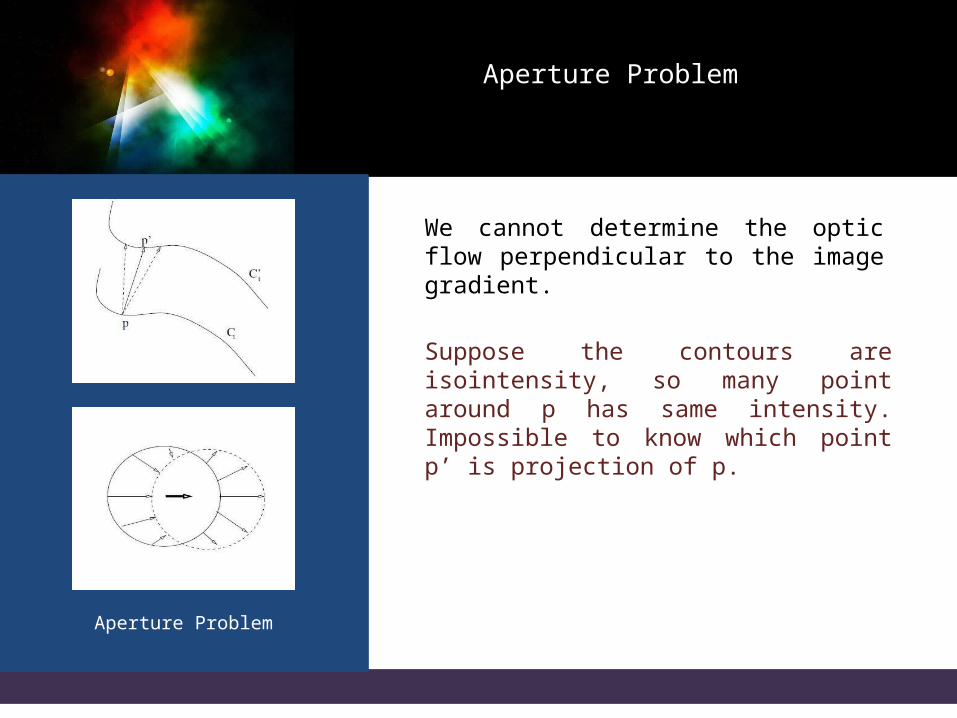
Given this constrain equation, we can only determine the normal flow, i.e., the flow along the direction of image gradient, but we can not determine those flow on the tangent direction of isointensity contour, i.e., the direction perpendicular to the image gradient. This is so called aperture problem.

Aperture Problem

Aperture Problem

We cannot determine the optic flow perpendicular to the image gradient.

Suppose the contours are isointensity, so many point around p has same intensity. Impossible to know which point p’ is projection of p.

Aperture Problem

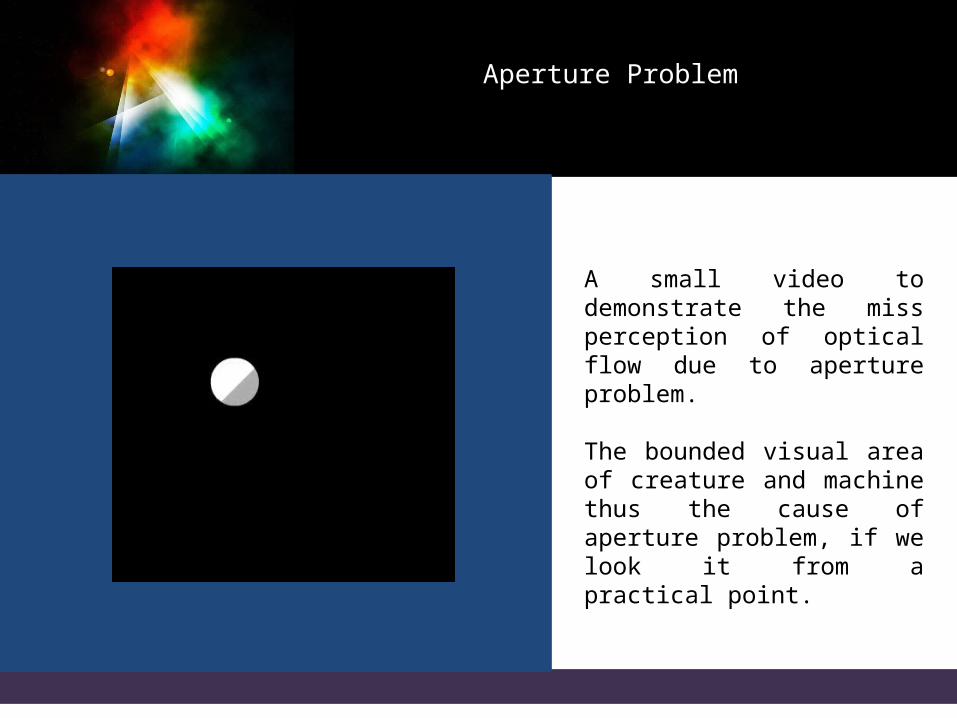
A small video to demonstrate the miss perception of optical flow due to aperture problem.

The bounded visual area of creature and machine thus the cause of aperture problem, if we look it from a practical point.

Horn and Schunck Model

Assumption : Optical flow varies flowObviously a global requirement

The measure of difference from smoothness is

The error of optical flow is


So we need to minimize

Use the four neighbor to find the discrete equivalent of the errors


So we need to minimize

Calculating the derivatives


are the local average of

Using an iterative method


For each iteration, the new optical flow field is constrained by its local average and the optical flow

constraints.Introduces a regularization term and a global

method

Locas and Kanade Model

Assumption : Optical flow can be described by a constant model in a small window Ω. We define a window function W(m), where m belongs to the window Ω. The weight for the center is greater than the others, thus the window favors the center.The optical flow of the center flow is thus calculated by

Writing out the derivatives


To solve it


Solving

Using notation


Note

The solution can be obtained when B is non-singular. Also the quality of flow estimation depends on the Eigen values of B. If they are sufficiently distant then the quality can be assured with confidence, with the decrease the quality falls and becomes impossible to determine when the smaller Eigen value becomes 0.

Lucas-Kanade method calculate the flow of a point m by identifying an intersection of all the flow constraint lines corresponding to the image pixels within the window of m. Those flow constraint lines will have an intersection, since this method assumes that the flow within the window is constant.

NeurosciencePerspective

Hubel & Wiesel (1968) describe cells in monkey’s striate cortex to be selective to bar movements.

Cells are also selective to moving lines of variable length called end-stopping or the line ends of such moving lines (Pack et al., 2003; Yazdanbakhsh & Livingstone, 2006). Motion detection based on such line ends is not affected by the ambiguity of motion for an edge, which is imposed by an aperture of limited size.

neurons in V1 are speed tuned. Their firing rate is invariant with respect to the spatial frequency of a presented sinusoidal grating, but varies with the contrast of the grating (Priebe et al., 2006).

NeurosciencePerspective

Signals of these motion selective cells are spatially integrated in the brain middle temporal (MT) area, which succeeds area V1 in the hierarchy of brain areas. This spatial integration is expressed by varying receptive field sizes: Receptive fields in area MT are about ten times as large as those of area V1 (Angelucci et al., 2005). Area MT cells span a wider range of speed selectivity, and have a broader direction (mean 95°) tuning compared to V1 cells (mean 68°). Some MT cells have the inhibitory region of different useful shapes to guide a partial derivation. fMRI also suggested high activity in different notable visual area at the time of optic flow stimulation.

Biological Inspired Modeling

The rabbit's retina uses a mechanism of inhibition. All non-preferred motions or all null-directions are inhibited. As a result, excitation remains for the presented potion. Inhibition could be generated by using de-correlation.

Correlation mechanism used by flies correlates preferred motion. Local image structure is detected at each location in the image. Detected structures from two spatially distant locations are correlated while signals from one location are temporally delayed. For instance, if the two locations are 2° of visual angle apart in the visual field and the delay amounts to 200 msec, then a motion speed of 10°/sec is detected in the direction determined by the arrangement of the two spatially distant locations in the visual field.

Simoncelli & Heeger (1998)

Visual area V1 and middle temporal area MT takes an important part in higher processing for developed primate cortical visual system. Step 1 : Area V1 detects initial motions by sampling the spatio-temporal frequency space with Gabor filters.Step 2 : Filtering results are squared, half-wave rectified, and then normalized to model the result of V1 simple cells.Step 3 : Responses of V1 complex cells are computed as the weighted sum of spatially neighboring simple cells with the same frequency and orientation.Step 4 : Model area MT cells sum V1 complex cell responses for all orientations and all frequencies that fall within a plane that corresponds to a velocity vector.Step 5 : A half-wave rectification, squaring, and normalization over neighboring spatial locations are computed for these model area MT cells.

Nowlan & Sejnowski(1995)

Step 1 : Retinal stage contains a DOG filter.Step 2 : Motion energy is detected using the model of Adelson & Bergen (1985) for four directions combined with nine spatial and temporal frequencies.Step 3 : The next stage combines these responses by sampling all frequencies that fall into a plane compatible with a single motion and uses eight directions combined with four speeds plus a zero velocity. In total, this gives 33 motion velocities or features say.Step 4 : Filtering results for these velocities are passed through a soft-max operation, which allows for the representation of motion transparencyStep 5 : Selectively chooses from these soft-max processed filtering results to compute a single velocity estimate as output by combining estimates from all spatial locations.

References

I. Florian Raudies, “Optic Flow”, from Scholarpedia, accessed on 17.0.3.2014.

II. Ying Wu, “Optic flow and motion analysis”, a tutorial, Advanced Computer Vision, Northwestern University.

III. “Aperture Problem”, a video active demonstration. MIT.

Thank You!

optic flow

Documents