optical mapping of crack tip deformations using the...

International Journal of Fracture 52: 91-117, 1991. © 1991 Kluwer Academic Publishers. Printed in the Netherlands.

Optical mapping of crack tip deformations using the methods of transmission and reflection coherent gradient sensing: a study of crack tip K-dominance

HAREESH V. TIPPUR 1, SRIDHAR KRISHNASWAMY 2 and ARES J. ROSAKIS Graduate Aeronautical Laboratories, California Institute of Technology, Pasadena, CA 91125, USA.

Received 20 November 1989; accepted 25 July 1990

Abstract. A new full field optical technique - 'Coherent Gradient Sensing' (CGS) - is developed and used to study crack tip deformations in transparent as well as opaque solids. A first order diffraction analysis is provided for the technique and its feasibility is demonstrated both in transmission and reflection modes. Preliminary results from the dynamic crack growth experiment clearly demonstrate the capability of CGS to be an effective experimental alternative to other optical methods used in dynamic fracture studies. Notably, it is a full field technique which works with optically isotropic materials.

The static fringe patterns obtained from the experiments are analyzed in regions outside the 3-D zone. For geometries where the region outside the 3-D zone is K-dominant, the fringes provide an accurate value of 2-D stress intensity factor. For geometries where the region outside the 3-D zone is not K-dominant, Williams' expansion is used in conjunction with a least squares procedure to obtain the stress intensity factors.

1. Introduction

In this paper, we report an experimental investigation of crack tip deformations in transparent and opaque solids using a new coherent optical technique - 'Coherent Gradient Sensing' (CGS). CGS is a full field, lateral shearing interferometric method. This full field optical method will be demonstrated both in transmission and in reflection modes to study deformations in transparent as well as opaque solids. Its ability to produce fringes in real time is used advantageously to map crack tip deformations in PMMA and A1 6061 specimens. The technique measures either in- plane stress gradients (transmission) or out-of-plane displacement gradients (reflection). CGS has a distinct advantage because of its insensitivity to rigid body translations and rotations which are generally quite difficult to avoid in experiments.

In the past, several other experimental procedures have been proposed for measuring surface slopes. Incoherent optical techniques such as reflection moir6 [1] and moir6 deflectometry I-2] are commonly used. Among the coherent techniques, defocussed laser speckle photography [3], grating shearing interferometry I-4], speckle shearing interferometry [5, 6] are some of the examples. Many of these methods have been demonstrated with either reflective or diffused object surfaces. Also, they typically consist of double exposure procedure which often is a limitation for dynamic applications.

In experimental fracture studies, photoelasticity I-7-9], caustics 1-10-14], geometric moir6 [15] and moir6 interferometry [16] are some of the methods used to measure crack tip deformations or deformation related quantities and hence the stress intensity factor. In these techniques,

1Currently with Department of Mechanical Engineering, Auburn University, Auburn, Alabama 36849, USA; 2Currently with Department of Mechanical Engineering, Northwestern University, Evanston 60201, Illinois, USA;

92 Hareesh V. Tippur et al.

interpretation of the measurements is based on the premise that a K-dominant, 2-D asymptotic field description exists in the vicinity of the crack tip. However, in reality, the situation has not been this simple. Recent studies have brought to light the shortcomings of such interpretations because of the three-dimensional nature of the crack tip deformation and the inadequacy of r -1/2 singularity term to model the field outside the three-dimensional zone (lack of K- dominance). In photoelastic studies, higher order terms have been used to overcome this lack of K-dominance [-8] in the interpretation of the experimental data. Rosakis and Ravi-Chandar [14], using the method of caustics, have addressed the question of crack tip three dimensionality. They showed that the caustics obtained from within the region of crack tip three- dimensional deformations (up to about one half plate thickness) could result in erroneous values of measured stress intensity factors. These results were supported by the analytical investigation of Yang and Freund [17]. Several finite element simulations performed since then [18-21] have further confirmed the three dimensional nature of the crack tip deformation field.

From these experimental and numerical investigations, it has become increasingly evident that a 2-D, K-dominant, crack tip field description for general specimen configurations should be used cautiously keeping in mind the near tip three dimensionality and possible lack of K-dominance. Furthermore, in dynamic loading situations, these complexities are compounded by the transient nature of the fracture phenomenon which may inhibit the establishment of a K-dominant region [21]. In view of the above, besides demonstrating the applicability of CGS to static and dynamic fracture studies, we will also examine some aspects concerned with the lack of K-dominance.

2. Experimental method

2.1. Experimental set-up

In Fig. 1 the schematic of the experimental set-up used for transmission CGS is shown. A transparent, optically isotropic specimen is illuminated by a collimated bundle of coherent laser

Specimen

jx~ I~

Grating G2

iz ix,",.

* jl / r .

t +. / / ,,

Fil~er Plane ' \ {

Imaging Lens L2 ~'j I 1

Imago Plane ~. i

Fig. 1. Schematic of the experimental set-up for transmission CGS.

Optical mapping of crack tip deformations 93

light. The transmitted object wave is then incident on a pair of high density Ronchi gratings, G1 and G2, separated by a distance A. The field distribution on the G2 plane is spatially filtered by the filtering lens L1 and its frequency content is displayed on its back focal plane. By locating a filtering aperture around either the _+ 1 diffraction orders, information regarding the stress gradients is obtained on the image plane of the lens L2.

Figure 2 shows the modification of the above set-up for measuring surface deflections of opaque solids when studied in reflection mode. In this case, the specularly reflecting object surface is illuminated by a collimated beam of laser light using a beam splitter. The reflected beam, as in the previous case, gets processed through the optical arrangement which is identical to the one shown in Fig. 1.

In the following sections, a first order diffraction analysis is presented to demonstrate that the information displayed on the image plane indeed corresponds to gradients of in-plane stress and gradients of out-of-plane displacement.

2.2. Principle

Figure 3 explains the working principle of the method of CGS. For the sake of simplicity, and without losing generality, the line gratings are assumed to have a sinusoidal transmittance. Let the gratings G1 and G2 have their rulings parallel to, say, the xx-axis. A plane wave transmitted through or reflected from an undeform~d specimen and propagating along the optical axis, is diffracted into three plane wave fronts Eo, E1 and E_ 1 by the first grating G1. The magnitude of the angle between the propagation directions of Eo and E± ~ is given by the diffraction equation 0 -- sin-~(2/p), where 2 is the wave length and p is the grating pitch. Upon incidence on the second grating G2, the wave fronts are further diffracted into Era,o), Em,~) , E u _ ~), Etl,o), ERE1) etc. These wave fronts which are propagating in distinctly different directions, are then brought to focus at spatially separated diffraction spots on the back focal plane of the filtering lens. The spacing between these diffraction spots is directly proportional to sin 0 or inversely proportional to the grating pitch p.

x2

Speo

Imaging Le

Image Plane

Fig. 2. Schematic of the experimental set-up for reflection CGS.


x 2 " x 2 -

o 2 . . . . .

Filtering Lens Filler Plane

Fig. 3. Schematic describing the working principle of CGS.

Now, consider a plane wave normally incident on a deformed specimen surface. The resulting transmitted or reflected wave front will be distorted either due to changes of refractive index or due to surface deformations. This object wave front that is incident on G1 now carries information regarding the specimen deformation, and consists of light rays travelling with perturbations to their initial direction parallel to the optical axis. If a large portion of such a bundle of light has rays nearly parallel to the optical axis, each of

the diffraction spots on the focal plane of L1 will be locally surrounded by a halo of dispersed light field due to the deflected rays. The extent of this depends on the nature of the deformations. By using a two-dimensional aperture at the filtering plane, information existing around one of the spots can be further imaged. Here, an important but subtle point should be noted. Since each of the diffraction spots is surrounded by dispersed light due to the deformation, overlapping of the information could occur on the filtering plane when the deflection of the ray is sufficiently large (i.e., >~ (2/2p)). However, it will be shown in the following sections, this limitation can easily be overcome by the use of higher density gratings.

2.3. Analysis

Consider a specimen whose midplane, in transmission, or surface, in reflection, occupies the (xx, x2) plane in the undeformed state. Let el denote unit vector along xcaxis, (i = 1, 2, 3), see Fig. 4. When the specimen is undeformed, the unit object wave propagation vector

do = e3. After deformation, the propagation vector is perturbed and can be expressed by,

do = ~el + fie2 + 7e3, (1)

where ~(xl, X2), fl(X1, X2), and 7(xl, X2) denote the direction cosines of the perturbed wave front. This upon incidence on G1, whose principal direction is parallel to, say, the x2-axis, is split into three wave fronts propagating along do, d+l and whose amplitudes Eo(x'), E+l(x') can be

represented by,

Eo(x') = ao exp[ikdo'x'], E~ l(x') = a . 1 exp[ikd+ 1 "x'], (2)


x 2 "

i e2 " a°E.~2_o

i~ ~ EO,1 ~o ~ ~E1, 0

Fig. 4. Diffraction of a generic ray in CGS.

where a0 and a±~ are constants and k = 2x/2 is the wave number. Due to diffraction by the

sinusoidal grating G~, the propagation directions of the diffracted wave fronts can be related to the direction cosines of the incident propagation vector through, see [22] for details,

d+ x = [:tel + {fl cos 0 + ? sin 0)e 2 + (7 COS 0 + fl sin 0)e3] , (3)

using the diffraction condition 0 = sin-l(2/p). On the plane G2(x'3 =A), see Fig. 4, the amplitude distribution of the three diffracted wave fronts are,

Eolx;=A = Eo(OTB) = aoexpEikdo.OTB] = aoexpEik(~)], {4}

Exlx;=a = E~{OTA) = al exp[ikdl '07,43 = al exp ik {7 cos0 - - [ J s in 0j ' {5)

E A i] E llx~=~= E-~( 07B ' j=a- l exp[ i kd ~'07B '] = a ~exp ik(TcosO+/JsinO ' {6)

The wave fronts Eo, E± 1 will undergo further diffraction upon incidence on G 2 into secondary

wave fronts E(o.o, EIo.1 ), E(I . -1}, E{1.oD E{1.1} etc. Of these secondary diffractions, E{o,l~ and E~l.o~ have their propagation direction along dl, E{o, ~} and E{_ l.O} along d ~ and Eo.o}, E{_ ~,l~ and E{~_ ~} along do, Fig. 3. If information is spatially filtered by blocking all but _+ 1 diffraction

order, only the wave fronts E(o.± ~} and E~± 1.01 contribute to the formation of the image. Noting that the two wave fronts do not acquire any additional relative phase differences after G2, the amplitude distribution on the image plane is,

E ,] E ~ m = ( E o + E + l ) l ~ , ~ = a o e x p ik +a±~exp ik(TcosOT_flsin 0 . (7)


Hence, the intensity distribution on the image plane is,

[ ._FT(cos 0 - 1)-T- fl sin 0]~ I,m = E,mE*m = ag + a~l + 2aoa+, cos~Ka L- ~T'/cos0 T fis~n~ J J ' (8)

where E% is the complex conjugate of Ei,,. Under small 0 approximation, the above equation simplifies to

i ,o = + a +l + aaoa+lcos t9t

Thus, lira denotes an intensity variation on the image plane whose maxima occur when

ka O °,2 - 2 n n , n = 0 , _+1, _+2 .... (10) /

where n denotes fringe orders. Similarly, when the principal direction of the grating is parallel to the xx-axis, it can be shown that,

kAaO 72 - 2 m m m = 0 , +1, + 2 .... (11)

Equations (10) and (l l) are the governing equations for the method of CGS and they relate fringe orders to the direction cosines of the object wave front. It is clear from the above two equations that the sensitivity of the method could be increased by either increasing the grating separation distance A or decreasing the grating pitch p.

2.4. Relation between direction cosines and deformation

We now relate the direction cosines of the object wave front to deformation quantities of interest for both transmission and reflection cases.

2.4.1. Transmission Consider a planar wave front incident normal to an optically isotropic, transparent plate of uniform nominal thickness h and refractive index no. Now, if the plate is deformed, the transmitted wave front acquires an optical path change 3S which is given by the elasto-optical equation (14),

f0 /2 t 1/2 6S(xl, x2) = 2h(no - l) g33d(x3/h) + 2h 3nod(x3/h). (12) do

The first term represents the net optical path difference due to the plate thickness change caused by the strain component g33. The second term is due to the stress induced change in the

Optical mappin9 of crack tip deformations 97

refractive index of the material. This change in the refractive index c~no is given by the Maxwell

relation,

6no(xl,x2) = O1(a11 + a22 + a33),

where D~ is the stress-optic constant and au are stress components. For an isotropic, linear elastic solid, strain component e33 can be related to stresses and thus (12) can be written as,

v jo

where D2 = [vD1 + (v(no- 1)/E]/[D1- (v(no- 1)/E], E and v are Young's modulus and Poisson's ratio of the material, respectively. The above equation is written in such a way that the second term in the square brackets represents the degree of plane strain. When plane stress is a good approximation, this term can be neglected and (13) reduces to,

6S ~ ch(t711 -'k d22), (14)

where c = D~ - (v/E)(no - 1) and t711 and t722 are thickness averages of stress components of the material. Using these, the propagation vector for a perturbed wave front can be expressed as,

o(6s) o(6s) V(S) 63x~ - e l + O x ~ e2 + e3

nO IV(S)] 1 -'{- k, 6qX1 / -+- k, 6~X2 J

o(6s) ~(6s) axe-el + Ox~-e2 + e3 (15)

for ]V(6S)] 2 ~ 1 and where S(xl, x2, xa) = x3 + 6S(xl, x2) = constant. Using (14) in (15), we can obtain the direction cosines of the propagation vector. Thus, using (10) and (11), the fringes can be related to the gradients of (~11 + 422) as follows:

ch O(all + (T22) mp ~" (16) 0Xl A '

~((711 "~ •22) np ch ~x2 ~ A' (17)

2.4.2. Reflection Consider a specimen whose reflective surface occupies the (xl, x2) plane in the undeformed state, Fig. 4. Upon deformation, the reflector can be expressed as

F(x1, x2, x3) = x3 q- /-/3(X1, X2) = O, (18)

98 Hareesh V. Ttppur et al.

where u3 is the out-of-plane displacement component. The unit surface normal N at a generic point O(xx, x2) is given by,

VF u3. te 1 + u3,2e 2 + e 3 N - - , (19)

2 2 IVFr x/1 + //3.1 + //3~2

u3,= implies differentiation with respect to x~. Consider now, a plane wave which is incident on

the specimen along the x3 direction. Let do be the unit vector along the reflected ray whose

direction cosines are ~, fl and 7. From the law of reflection, and noting that vectors do, N and e3 are coplanar, one can show that [22] the direction cosines of do can be related to the gradients

of u3 by,

- - U 3 , 1 - - / / 3 . 2 ) ( 2 0 ) 2u3,1 2U3, 2 , )' (1 2 2 2 2 ' f l ~ 2 2 = 2 2 '

= (1 + //3,1 + //3,2) (1 + //3,1 -~- U3,2) (1 + U3,1 + U3,2)

Using the above in (10) and (11), and using ]Vu3] 2 ~ l, we get,

~u3 (mp) " ~ m = 0 . + 1, + 2 , . ( 2 1 )

~x~ ~ . . . . .

~x2 ~ n = 0, _ 1, _+2 .... (22)

where the fact that 0 ~ (2/p) and k = 2~/2 are made use of. For an isotropic, linear elastic solid,

out-of-plane displacement u3 can be expressed as follows:

~0 '2 u3 = h c33(xl, x2, x3)d(x3/'h)

(23)

In the above, the second term in the square brackets represents the degree of plane strain and

when plane stress is a good approximation, it can be neglected. Thus, the above equation

reduces to,

vh U3 = - - ~ ( 6 1 1 + ~22)' (24)

Hence (21) and (22) can be expressed as,

(}/33__ vh ~ ( d t l +#22){mp~ ~xl 2E ~xl ~J2A

m = 0 , _+1, _+2 .... (25)

e//3 ,,I, + a 2 2 1 ( , , q ?x2- 2E ?x2 \ 2 A ]

n = O , + I , _+2,... (26)

Optical mappino of crack tip deformations 99

3. Experiments

3.1. Spherical wave front

To verify the above diffraction analysis, first we carried out an experiment in which a well defined wave front is studied. A spherical wave front is generated by passing a collimated beam of light through a convex lens of focal length ft. The spherical wave front emerging from the

convex lens can be described by,

( ~ S ( x 1 , X 2 ) - - _ _ 2f,

Hence, the propagation vector is,

V S X 1 X 2 = 7 < + + e , ,

~J ~J

where S(xa, Xz, x3) = x3 + 6S(xl, Xz) = constant. When grating lines are oriented such that their principal direction is parallel to the x2-axis, we obtain,

x2 np (27) f l - f , - A"

Thus, the filtered image consists of equally spaced parallel fringes as shown in Fig. 5. For the experimental parameters of ft = 546 mm, p = 25 Ixm and A = 22 mm, the expected fringe spacing (x2/n) is 0.66 mm/fringe and is in good agreement with the experimental observation of 0.63 mm/fringe.

3.2. Three point bend fracture specimens in transmission

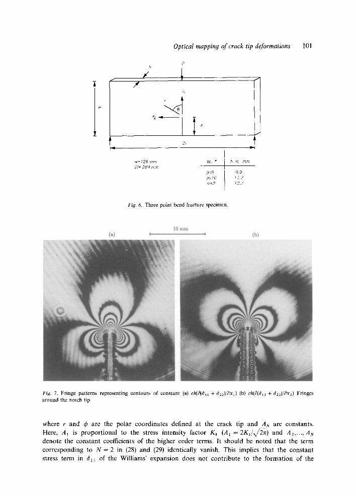
Specimens are made from a sheet of PMMA of thickness 9 mm for studying crack tip fields. The specimen geometry and the three point bend loading configuration used is shown in Fig. 6. Three different crack length (a) to plate width (w) ratios, namely (a/w) = 0.2, 0.32 and 0.52, are studied. A band saw, approximately 0.75 mm thick, is used to cut notches in these specimens. A collimated laser beam of diameter 50 mm is centered around the crack tip and transmitted through the specimens in these experiments. The object wave front is processed through a pair of line gratings of density 40 lines per mm with a separation distance A = 30 mm. Figure 7 shows the fringes around the crack tip when the grating lines are perpendicular to the xl- and x2-axes, respectively, for an applied load P = 1775 N. These fringes represent contour maps of constant [O(6S)/dXl ], [-~(6S)/Ox2] , respectively, where 6S is the integrated optical path difference through the specimen thickness, see (13). In the regions around the crack tip where plane stress is a good approximation, these reduce to ch(O(6~ + 622)/0x0, ch(~(611 + 622)/c~x2). For the experimental parameters chosen, the sensitivity of measurement is typically 0.025 degree/fringe. It is apparent from these patterns that CGS produces sharp and high contrast fringe patterns in the near vicinity of the crack tip. The numerical aperture [F t#~] of the optical system used in the

100 Hareesh V. T ippur et al.

Fig. 5. x2-derivatives of a spherical wave front.

study limits the maximum deflection that could be measured to about 0.8 degrees, and deflections greater than this do not reach the image plane, leading to the formation of a small dark spot around the crack tip.

To analyze the crack tip deformation fringes, we assume a linear elastic asymptotic plane stress field to prevail in the crack tip vicinity. Using Williams' expansion [-23] for a mode-I crack

stress field in (16) and (17), we find,

ch(~(~ll q- (722) ch A N ~ - I r (0'/2)-2~ COS ~ - - 2 ~b = ~- , (28) Oxt N = I

ch~(611 + ~ 2 2 ) __ ch y~ AN ~ -- 1 r ~N/2)-2) sin -- 2 ~b = (29) ~x2 A ' N = I


h

_ _ J P

x I

21

1 w = 1 2 6 mm 21= 2 8 4 mm

sp. # h in mm

ps9 9.0 p s l O 1 1 7 ms2 1 2 7

Fig. 6. Three point bend fracture specimen.

Fig. 7. Fringe patterns representing contours of constant (a) ch(~3(dll + d22)/~X1) (b) ch(0(611 + 622)/~x2) Fringes around the notch tip.

where r and ~b are the polar coordinates defined at the crack tip and AN are constants. Here, A1 is proportional to the stress intensity factor K~ (A1 = 2 K ~ / x ~ ) and A2 ..... An denote the constant coefficients of the higher order terms. It should be noted that the term corresponding to N = 2 in (28) and (29) identically vanish. This implies that the constant stress term in ~11 of the Williams' expansion does not contribute to the formation of the


fringes. This feature, which is also present in the method of caustics, could be an advantage if a single parameter fit of the experimental data is sought. Also, this constant term has been shown to be responsible for tilting of the crack tip fringes in the method of photoelasticity.

Let us, now, define a K-dominant crack tip field as one in which the contribution from N >~ 2 terms is negligible compared to the first term. Thus, when a K-dominant field exists near the crack tip, (28) and (29) reduce to,

Kl 3 ~ /~/P oh- ~ r - " '~ cos(3~b/2) + O(r- 1:2) = A-' w,"2~

(30)

ch-~rx/2~z 3/2 sin(3~b/2) + O(r- ~.,2) = A-'nP (31)

where the negative sign has been absorbed in to fringe orders m and n. Now let us define two functions Y~ and yIz) a s follows:

Y~l~(r, 4)) = ch cos(3qS/2)' (32)

,.3..2

ch sin(3~b/2)" (33)

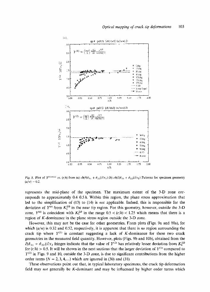
It is apparent from the above two equations that when a K-dominant field adequately describes crack tip deformations, then Y~ (~ = 1,2) is identically equal to the mode-I stress intensity factor K~. To measure Y~) from fringe patterns, the pictures are digitized and fringe order (m or n) and radial distance (r) along different directions (4~) around the crack tip are tabulated. Functions Y~'I are plotted against normalized radial distance (r/h) for different crack length to plate width ratios (a/w) in Figs. 8 10. The calculated K~ measured from the applied load measurements is indicated as K~ D, see [-24]. Several interesting observations can be made from these plots. If a K-dominant field were to exist in the near tip region, one would expect Y~'~ to be constant in each case and equal to K 2~ to within experimental

error. Indeed, as seen in Figs. 8a, b, for certain geometries (a/w = 0.2), there seems to be a region of constant Y~'~ when 0.5 < (r/h) < 1.25. The value of this constant is also equal to K~ D to within about 10 percent. Also, when (r/h) < 0.5, the data seem to underestimate the value of K 2D by more than the typical experimental errors that one would anticipate. This observation is consistent with other experimental investigations [14,9, 15] wherein such behavior has been attributed to 3-D deformations near the crack tip. In recent times, several finite element calculations [18-21] have also confirmed the existence of the 3-D zone surrounding the crack tip. Figure 11 shows a 3-D representation of the degree of plane strain [~33/v(~1 + a22)] which is a measure of the near tip three dimensionality. This corresponds to a 3-D finite element simulation [21] of the geometry used in these experiments. In regions where deformation is locally plane stress, this measure is equal to zero. In the figure, only one half of the specimen thickness is shown. The top surface


g.

3 . 0

2 .5

2,0

s p . # p s 9 / 6 [ d f / d x l ] ( a / w = 0 2 )

= ch c o s ( 3 o / 2 )

. . . . . _dLe'£t~ .~_ 21~" al = ~ - :z t,.u. . . . . . ¢ . . . . ~ . . . . . . . .

Y []

] ~ ] ] ' I l I ' l

0 . 2 5 0 . 5 0 0 ,75 1 .00 1 .25

r / h

1 ,5

1 .0

0 .5

0.{ u.O0

t~ 0deg + l S d e g

3 0 d e g

• 45de g

[] 105 deg

120 deg 6 135 de g

.......... K.2D

- - " K.exp (3-par)

- . e - K-caus

1 .50 1 .75 2 .00

( h ) . s p . # p s 9 / 5 [ d f / d x 2 ] ( a l w - - 0 2 )

3 ,0 [ - , . . . , . , • , " i • , -

2.s " - ~ a; ~/, ~ i

2.0

o 30deg 1.5

I . . . . . . . . . . . . . . . . . . . . . . . . . . . . . . . . :"v::'* .7 .................................................................................. , , 45 deg

I ~ u 60 deg 1.0 ~ ~ 75 deg

0 @ • 9~dL~g

0 .5 .......... K-2D

- . o - K-caus

0.01 , i , I , i i i , ~ , i , i ,

u . 0 0 0 . 2 5 0 . 5 0 0 . 7 5 1 .00 1 .25 1 .50 1 ,75

r / h

ZOO

Fig. 8. Plot of y(l)or(2) vs, (r/h) from (a) ch(0(611 + 6zz)/dxl) (b) ch(8(611 + dzz)/Ox2) Patterns for specimen geometry (a/w) = 0,2.

represents the mid-plane of the specimen. The maximum extent of the 3-D zone corresponds to approximately 0.44).5 h. Within this region, the plane stress approximation that led to the simplification of (13) to (14) is not applicable. Indeed, this is responsible for the deviation of Y~') from K~ ° in the near tip region. For this geometry, however, outside the 3-D zone, Y(') is coincident with K2~ ° in the range 0.5 < (r/h) < 1.25 which means that there is a region of K-dominance in the plane stress region outside the 3-D zone.

However, this may not be the case for other geometries. From plots (Figs. 9a and 10a), for which (a/w) is 0.32 and 0.52, respectively, it is apparent that there is no region surrounding the crack tip where ym is constant suggesting a lack of K-dominance for these two crack geometries in the measured field quantity. However, plots (Figs. 9b and 10b), obtained from the •(ffll "~ ~22)/(~X2 fringes indicate that the value of y(2) has relatively lesser deviation from K~ z° for (r/h) > 0.5. It will be shown in the next sections that the larger deviation of ym compared to y(2) in Figs. 9 and 10, outside the 3-D zone, is due to significant contributions from the higher order terms (N = 2, 3, 4 .... ) which are ignored in (30) and (31).

These observations point out that, in typical laboratory specimens, the crack tip deformation field may not generally be K-dominant and may be influenced by higher order terms which

104 Hareesh V. Tippur el al.

£ ,.<

IE

L

3.0

25

2 tl

1.5

]{)

ti5

(]0 u[}O

! , ?

30 .

25

2 0

15

] 0

0U u t)0

sp.# ps9/21 (a/w=0.32)

D D ,' deg o

+ + 15deg o

o 3a deg + D

- e o 45 deg

" ~ A x ~:k A~ . . . . . . . . . . . . . . . . . . . . . . . . . . . . . . . . . . = 103dcg

Ae~ =- 'al~'~ nn x x 120deg

A 135 deg

.......... K2D

- - - K exp (3 par)

- e , - k caus

i i , i , i , i i i

0.25 l ist ] 0.75 10{1 1.25 1.50 [ 75

r / h

sp.# ps9/22 (a/w:O.32)

i

. . . . . . . . . . . . . . . . . . . . . . . . . . . _ _ W ~ . ~ . . . l ....................................... , a . . . . . . . . . . . . . . . . . . . . . . . . . . . . . . . . . . . . . . . . . . . . . . . . . . . . . . . . . . . a . • 45 deg

# ' ° ~ " 60deg

~ N 75 deg

i 9 ) d e g

.......... K-2D

- . e - K ca,as

D25 {150 075 1( i / ] 2 5 ]50 175

r , / h

2(kl

2 t](]

Fi9. 9. Plot of y{1}or{2) VS. (r/h) from (a) ch(?(~11 + 622)/(~x1) (b) ch(?(d~ + d2j/Ox2) Patterns for specimen geometry (a/'w) = 0.32.

should be accounted for, if K~ is to be extracted from regions outside the three dimensional deformation zone. However, there may be exceptions to this, as in the case of the specimen with (a/w)= 0.2, where one can measure K~ quite precisely without resorting to the use of higher order expansion. The use of higher order terms has also been found to be necessary in photoelastic fracture studies (for example, see [-8]). In the next section we attempt a data analysis procedure using a multi-parameter, least square curve fitting to determine K].

Another interesting observation could be made about the data corresponding to 4} -,~ 120 ° in Figs. 8-10. Although, substantial deviations in the measured values of Y{~} seem to persist along different radial lines, the variation along ~ ~ 120 ° is the least in all of the cases considered. Moreover, the data seem to be in good agreement with the corresponding K2Q Although this may seem surprising, it is consistent with the behavior shown in Fig. 11. Indeed, along ~b ~ 120 °, the extent of the 3-D zone seems to be the least. Because one can closely approach the crack tip (say, up to about 0.25 h) along 4} ~ 120 c' without being affected by near tip three dimensionality, the deformations in this plane stress region are relatively less influenced by the higher order terms.


( b ) .

3.0 • , • ,

2.5

2.0

1.5

l .o

0.5

O.G u.00

(a) .

s p . # p s 9 / 2 4 ( a / w = 0 . 5 2 )

3"01 . . . . . . . . • . . . . . . . /

2.01- • o + ~ u 0deg |

+ 15deg l +~ o 3 0 d e g

1.5~ • # o " ' ' ' ~ ' ' ' ' ' ' ~ ' ~ • 45deg

I • o ~ a . . . . . . [] 105deg - - - - ~ - ~ - - - ~ , . . . . . . . . . . . . . . .

1.0 . . . . . . . . . . . . . . . . . . . . . . . . . . . . . . . . . . . . . . . . . . . . . . . . . . . . . . . . . . ~ " ~ ............................................... x 120 deg l ~ A I35 deg [ ~ .......... K-2D

0 . 5 [ --e- K-caus i

- - - K-exp G-par) 0 . 0 / , J , I , I , I , I , I i

u.00 0.25 0.50 0.75 1.00 1.25 1.50 1.75 2.00 r / h

sp.# p s 9 / 2 5 ( a / w = 0 . 5 2 )

d N II "~ o • O - ~ m l o o 45deg _Q~, • 60 deg

o N 75 deg

• 90deg

.......... K-2D

--o- K-caus

i r i i , r l L

0.25 0.50 0.75 1.00 1,25 1.50 1.75

r / h

2.00

Fig. 10. Plot of y(1)or(2) vs. (r/h) from (a) ch(O(dal + 62z)/Ox 1) (b) ch(O(dll + d22)/(~X2) Patterns for specimen geometry (a/w) = 0.52.

3.2.1. Least square data analysis

In this section we describe a multi-parameter least square data processing to extract K] from regions outside the 3-D zone. The O(dl~ + d2z)/Sxl fringe patterns are used in this analysis because they show relatively larger deviations from K 2D in Figs 9-10. The fringe patterns are digitized around the crack tip to obtain fringe orders (m or n) and fringe location (r, ~b) around the crack tip. Typically the data from the t3(dx~ + ~zz)/Sx~ field is obtained for (r, 0 ° < ~b < 45 °) and (r, 90° < 4)< 150°); and from (r, 30° < ~b < 90 °) when t3(dll + ~22)/t~x2 field is used. The choice of the above ranges in q~ is simply guided by the most number of fringe intersections that occur in these sectors.

In the absence of K-dominance, from (28) we find,

ch cos(3~b/2) \ A J Z-" k AN ~ -- 1 r ((~¢- 1)/z) N= 1 cos(3~b/2) ' (34)


Fi O. 11. Degree of plane strain near the crack tip in a three point bending configuration (from [21]).

where the multiplicative constant ,/"2~ is absorbed into AN. Note that the left hand side

in the above equation is Y(~ and is proportional to At or KI for a K-dominant field and

consists of quantities that are measured from the fringe patterns. The right hand side of the above expression, denoted by FIll(r, qS;A1,A3 ..... AN), is the least squares fit we

would attempt for our experimental data. As explained earlier, the term associated with

N = 2 is identically equal to zero because it represents the gradients of constant stress and hence

does not contribute to our fringe patterns. In the curve fitting procedure, we minimize the

function,

M

OO(A1, A3 ..... A~.) = ~ qi[y~i '' _~F'I'] : j (35) i = l

with respect to A1, A3,...,A~-. Here, M is the total number of data points used in the

minimization and q is the weighting factor (q = 1.0 for 1hi or ImL > 1 and q = 0.95 for In1 or I ml ~< 1) which takes into account the uncertainty associated with the location of fringe centers. The satisfactory number of higher order terms needed for a good fit is determined by the


number of higher order terms which yields minimum value of the non-dimensional error function ~ defined as,

~(N) = . (36)

In the above procedure, experimental data from the 3-D zone, the radial spread of which is obtained from the plane strain constraint contours shown in Fig. 11, have been dis- regarded. Thus, the data primarily comes from regions (r/h)> 0.5 for 0 ° < ~b < 90 ° and 140 ° < ~b < 180 °. For qS = 105 ° and qS = 135 °, the extent of three dimensionality is assumed to be up to 0.4h and 0.25h along qS = 120 ° . Figure 12 shows the variation of e as the number of terms (N) used in the expansion is varied for the field quantity C(611 + 422)/0xl for different (a/w) ratios. Typically the error function attains a minimum as more number of terms are considered and begins to increase when more than optimal number of terms are used. This increase in ~ is because the function tries to improve the fit for those data points with larger degree of uncertainty in the wide outer fringe loops. Also, from this plot it is apparent that, when (a/w) = 0.2, ~ constantly increases with the number of terms (N) while for (a/w)= 0.32 and 0.52, ~ decreases upto N = 3, and increases when more terms are added. This implies that a three term expansion is necessary to describe the 2-D field surrounding the crack tip for (a/w)= 0.32 and 0.52 whereas just a single term expansion is sufficient for (a/w)= 0.2 confirming K-dominance observed outside the 3-D zone in that specimen. The values of K~ obtained by the above procedure are also shown in Figs 8-10. To provide a visual picture of the agreement between the multi-parameter fit and the experimental data, contours of C(dll + dz2)/Cxl are shown in Figs. 13a, b for (a/w)=0.2 and 0.52. The symbols denote raw experimental data from the fringe patterns. Here, solid lines represent multi-parameter fit while the broken lines represent single parameter description. The circle centered around the crack tip represents (rib = 0.5, 4). When (a/w)= 0.2, Fig. 13a, for which K-dominant description gives the lowest value of e, the data points are well described just by the single parameter fit. However, when (a/w)= 0.52, it is apparent that a three parameter expansion is essential. The three parameter description seems to help fit the digitized data fairly well all around the crack tip while a single parameter fit shows

0.5

0.4

0.3

0.2

0.1

0.0

, - - " ~ - p s g / 6 ( a /w- i ) . 2 ) o.,- . . . . -o-- . p s9 /21 ( a / w - 0 . 3 2 )

G . . . . <" '" p s 9 / 2 4 ( a /w=0 .52 )

,,,: -\ .::+o

• . . . . . . o . . . . . " " . . . . . . o - " . o . _ _ - - i t "

i i i i

2 4 6 8 10

Fig. 12. Error function e vs. number of higher order terms N for different crack geometries.


I \ . f ~'\ ,

~ *" "il

\ I

• ~ \ l - k l ~" ' i I i i N

~ ' ~ I ¢ / . ~ - ~ ~ 't-. ~ ~ ~

2:~<~ I \ ~._~ ~+

\ \+

\ \

\ +

I

/ I

\ / + /

"., i

÷

+ \ . t +

, ~ / / , , Y

I\@ ~ ,¢ ' j /+ / t ~1

+ ~ ] ! ~ - - - \ - "\+-~ +j l+ + I I I / /

f )

Fig. 13. Synthetic [ch(c~(6~a + d22)/(GXI)] contours from multi-parameter, least squares, data analysis; Solid-line: Three parameter fit (N = 3); Broken line: One parameter fit (N = 1); (a) (a/w) = 0.2 (b) [a/w) = 0.52. Crosses represent raw data used in the data analysis.

large deviations from the data points, Fig. 13b. Again, it should be noted that the data along q~ ~ 120 ° seem to fit the contours the best. In Fig. 14a we have superimposed the three parameter fit (shown as broken lines; note that the synthetic contours that are plotted correspond to both dark and light fringes) for (a/w)= 0.32 on the original fringe patterns demonstrating good agreement between the fit and the fringes outside the three dimensional region. Also, to verify the conformity in results between the two field quantities namely, ~((~11 ~- (~22)/GX1 and 0(611 + ~22)/~x2, in Fig. 14b we have shown the synthetic contours of c~(611 + d2z)/~x2 for (a/w)=0.32 using A~, A3 and A 4 obtained by processing the data from the corresponding (~(61~ +~22)/?.xl fringes and superposing it with the actual 0(611 + 622)/0x2 fringe pattern.

Next, let us examine why the spread in y(2) from c(~11 -t- ~22}/~x 2 field is less than those from ~(~11 "~ (~22)/CX1 fringe patterns. First note the difference that the digitized data come from different regions in the two fields. The ~(dl~ + dz2)/~xl patterns are digitized along (r, 0 ° < ~b < 45") and (r, 90 < q~ < 150 °) while ~(ff~ + 622)/?~x2 patterns are digitized in the range (r, 30 -~ < ~ < 90°). As stated earlier, this choice is simply guided by the fact that one can realize greater numbers of least erroneous fringe intersections along these directions. It was previously demonstrated that the field in this case (a/w = 0.52) can be well described with three terms rather than one term. Thus , for N = 3, F (u becomes ,

( cos +J2, r32 ' 1) F~X)(r, qS; A1, A3, A4) = AI 1 + ~ r c o s ( 3 q ~ / 2 ) + A1 cos(3q~/2i -~ At(1 + g(1)) (37)


Fi9. 14. (a/w)= 0.32; (a) Synthetic [ch(O(611 + ~22)/0X1)] patterns (broken lines) obtained from three parameter fit (N = 3) superposed on actual fringe patterns. (b) Synthetic [ch(O(dl i + ~22)/0x2)] patterns (broken lines) obtained from three parameter fit (N = 3) for [ch(t3(rH + ~22)/0xl)] and superposed on actual fringe patterns.

to describe the function y(1) at any generic point in the field. Similarly, if O(ff11 -1- ~22)/~X2 field were considered, one can write the counterpart of (37) as,

~A3 sin(q~/2) ~'~ F(2)(r, ~b; A1, A3, A4)= A~ 1 + [fiT r sin(34)/2)~ ) - A~(1 + 9 (2') (38)

to describe y(2). In (37) and (38), g") and g(2) represent the contribution of the higher order terms. Also, note that the term associated with N = 4 is identically equal to zero in ~ ( ~ + ~2z)/t3x2 field, (38). In Fig. 15, g(a) and 9 ~z) are plotted against ~b for (r/h) = 1 and the ratios (Aa/AO and (Ag/At) obtained from the least squares fit for the O(dll + ~22)/0xl fringes. The emphasized portions of the curves indicate the regions from which the data is typically extracted for the multi-parameter analysis. It is evident from these plots that as 4)---, 60 °, the contribution of gO) becomes much larger than unity in the ~(~11 + ~2z)/OXl field. Similarly, as ~b~ 120 °, the contribution of g(2) becomes large compared to unity in the 0(~1~ + ~22)/(~X2 field. Figure 15a indicates that in the t3(d~ + 622)/t3x~ field, the data ahead of the crack tip (0 ° < q~ < 45 °) will have larger contribution from g") than for those from behind the crack tip (90 ° < ~b < 150°). At the same time, the magnitude of 9 (z), Fig. 15b, is small compared to unity and varies weakly with ~b in the region where the experimental data are obtained (30 ° < ~b < 90°). This explains why the spread in Y") obtained from the data ahead of the crack tip in the 3(~ 1 -'1- d22)/0X1 field is more when compared to the data from behind the crack tip in Figs. 9-10. Also, magnitudes of AN/A1 are certainly an important factor which directly account for the overall contribution of g~) and g(2) and hence the deviation from K-dominance. This illustrates that the experimentally observed K-dominance depends not just on the region of measurement but also on the field quantity considered.


I.).

-1

- 2

(l~). 2

i (r/h)=1 (A3/A1)*h=0.43 (h4/A1)*(h**l.S)=0.0s

i

30

. f I ' "

t

I

i i i

60 90 i i

120 150 180

I

s

-2 i i i i i

0 30 60 90 120 150 180

Fig. 15. Higher order contributions g ( 1 ) o r l 2 ) VS . angle q~ for (a/w) = 0.52.

3.2.2. Synthetic caustics The caustic mapping in transmission is given by the relations [11],

x ' ,=x,+ Zo[ch ~(t711 -~- (722) 1 ?~x, ' ~ = 1,2, (39)

where (x'~, x~) denote the in-plane coordinates of the caustic plane located at a distance Zo from the specimen plane along the optical axis and (xl, x2) correspond to the in-plane co-ordinates of the specimen plane. From a multi-parameter analysis of the 0(611 + (722)/(~X1 patterns of CGS (refer to (34)) one can obtain A1, ... AN needed to evaluate ~(611 + ~22)/c3x~. Synthetic caustics are generated using the mapping relations (39) for a range of Zo leading to caustics obtained from different distances ro (initial curve radius) from the crack tip. In Fig. 16 one such caustic (Zo = 4.0m) obtained for (a/w) = 0.52 and a three term expansion (A1, A3, A4), is shown. Also, the values of K . . . . , measured by interpreting the synthetic caustics as if they were from a K-dominant region (only A1 present) are shown in plots in Figs. 8-10. Some interesting


. L i ," . . . . . . . . \ . . ~" t .."./.. •

....:.,, ....,,.~ . ~ 7..- • .., --......\ . / .:--

+**~.o+ +o+'~+ o~, + +

+ . +,-.~. *% ~ , + +

. . . . . . . .. . . ." k"'i~ • . . . . . . , , ' , .......:.... . .

. ..- ~ ~ , . "

h i i

Fi G 16. Synthetic caustic generated using the three parameter fit for [ch(0(611 + ~22)/~xl)] patterns [(a/w) = 0.52 and Zo = 4.0 m].

observations can be made from these results. For (a/w) = 0.2, Fig. 8a, b, for which K-dominance is observed through CGS outside the 3-D zone, the agreement between K 2° and K ca"*, for different initial curve radii in the range 0.4 < (ro/h) < 0.75, is good. When (a/w) = 0.32 and 0.52, we see that the magnitude of K ca"s, for the same range of initial curve radii as above, is apparently a constant. However, K . . . . overestimates K~ ° by as much as 50 percent. This is clearly a consequence of a lack of K-dominance. Also, note that K ea"s values coincide with a horizontal portion of y<2) obtained from the 0(fill + ~22)/0x2 pattern; however, both of them differ substantially from K 2°.

3.3. Three point bend fracture specimens in reflection

Applicability of CGS to opaque solids is demonstrated by using it in reflection mode, Fig. 2, to map surface deformations in single edge notch, three point bend specimen made of PMMA (plate thickness of l l .Tmm) and AI 6061 (plate thickness of 13mm, yield stress ao g 300 MPa). The specimen geometry is the same as the one used in transmission experiments, Fig. 6, with a notch length to plate width ratio of (a/w) -- 0.2 in which K-dominance is observed in both the derivative fields. One of the faces of the PMMA specimen is aluminized to provide a reflective surface. In the case of aluminum specimens, a flat mirror-life surface is produced by lapping one of the surfaces flat and subsequently polishing it to 1 gm finish to obtain a reflective surface.

The fringe patterns observed in reflection CGS by using the set up described earlier, are

shown in Figs. 17 and 18. As previously described in Section 2.4.2, they represent contours of constant surface gradients, ~u3/c~x~ where ua is the out-of-plane displacement component. Although the overall structure of these fringes is similar to those obtained in transmission experiments, there are some differences. The sensitivity of the fringes is 0.0125 degrees/fringe - twice that of transmission CGS for the same grating separation A. Clearly, in the case of aluminum specimen Fig. 18, dense and wiggly fringes concentrated around the tip of the notch

112 Hareesh V. T ippur et al.

Fig. 17. Fringe patterns representing contours of constant (a) ?m3/~xl (b) ~u3/Ox2 fringes around the notch tip; (PMMA in reflection).

Fig. 18. Fringe patterns representing contours of constant (a) Ou3/~xl (b) Ou3/Gx 2 fringes around the notch tip; (AI 6061-T6 in reflection).

indicate plastic deformat ion at the crack tip (plastic zone radius rp/h ~ 0.3). In any event, the

fringes close to the crack tip are still discernible and the method demonst ra tes its ability to a c c o m m o d a t e modera te amounts of plastic deformations.

In te rpre ta t ion of these fringes is done using Will iams' expansion [23] for mode- I crack stress

Optical mapping of crack tip deformations

field in (25) and (26) and we get,

rheA:N) m, 0-~xl= ~N~__ 1 N k ~ - ' l r((m2)- 2) cos ~ - - 2 q ~ - ~ ,

Ou3 v h ~ ( N ) ( N ) np = ~-Eu~=IAN ~ - 1 r ((m2)-2)sin ~ - 2 ~ b = ~ .

113

(40)

(41)

If a K-dominant field were to prevail near the crack tip, higher order terms in (40) and (41) can be neglected to yield,

8u3 vh K I _3/2COS(3t~/2 ) mp (42) ~x, = ~ qT~ r = ~ '

x~2n np (43) (~U 3 = Yh r - a / 2 s in (3~b /2 ) = ~ . ax2 2E

(a).

(b).

~q

4.0

3.5

3.0

2.5

2.0

1.5

1.0

0.5

0.0 u.00

s p . # p s l 0 / 9 ( d u 3 / d x l ) ( a / w = 0 . 2 )

Z (1) (-~A) 2 E v ' ~ r 3/2 = vh cos(3<b/2)

• + ~ + a °

. ~ u o + •

÷~

o l

i i i i

0m~ 0 . ~ 0"75 1.00

r / h

s 0deg

+ I5deg

o 30deg

• 45deg

u 105 deg

x 120 deg

A 135 deg

- - - K-2D

I 1 m25 1.50

4.0

3.5

3.0

2.5

2.0

1.5

1.0

0.5

sp.# pslO/lO [du3/dx2] (a/w=02)

z ~ (~) ~ *~'~ : vh sin(3qV2)

/ n~Im ++ • ,, •

0.0 i i i i

u.O0 0.25 0.50 0.75 1.00 r / h

o ~ d e g

• 45 deg

• 60deg

" 75deg

• 90deg

- - K-2D

n 1.25 1.50

Fig. 19. Plot of Z (~°r(2) vs. (r/h) obtained from (a) Ou3/Oxl (b) c~ua/Ox2 patterns for [(a/w) = 0.2] P M M A specimen.


40

30

20

10

0 u.O0

(a) ,

8O

7O

60

50

4O

3O

20

10

0 v,O0

( h i .

8O

70

60

50

sp .# m s 2 / 1 0 a ( d u 3 / d x l ) ( a / w = 0 . 2 )

D ÷ + tl o

o t~ x

, . , ~ d!~ ° - o ~ " " ÷ 15d~g o 30deg

~ 45deg

a 105 deg

x 120 deg

A 135 deg

......... K-2D

0.25 0.50 0,75 1,00 1,25 1.50 r / h

sp .# m s 2 / l l a [ d u 3 / d x 2 ] ( a / w = 0 . 2 )

o

ca o0 ~ x • M • i1 i ea

~ . . "" OSOdeg * 45deg mR II m 60deg

N 75 deg

90deg

.......... K-2D

, i, l r F I,,,

0.25 0.50 0.75 1.00 1~25 1,50 r / h

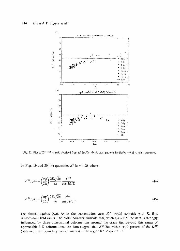
Fig. 20. P l o t o f Z m°~(2~ vs. (r/h) o b t a i n e d f r o m ( a ) i~u3/Ox 1 (b ) Ou3/gx2 p a t t e r n s f o r [(a/w) = 0 . 2 ] AI 6 0 6 1 s p e c i m e n ,

In Figs. 19 and 20, the quantities Z" (~t = 1, 2), where

rap) 2E~/~ r 3!2 Zm(r' 95) = ~ vh cos(395/2)' (44)

np) 2 E x / ~ r 3/2 Z(2)(r' 95) = ~ vh sin(395/2)' (45)

are plotted against (r/h). As in the transmission case, Z (') would coincide with Kx if a K-dominant field exists. The plots, however, indicate that, when r/h < 0.5, the data is strongly influenced by three dimensional deformations around the crack tip. Beyond this range of appreciable 3-D deformations, the data suggest that Z (') lies within _+ 10 percent of the K~ 2° (obtained from boundary measurements) in the region 0.5 < Uh < 0.75.


3.4. Demonstration of CGS in dynamic fracture

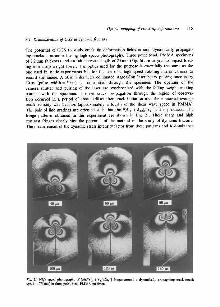
The potential of CGS to study crack tip deformation fields around dynamically propagating cracks is examined using high speed photography. Three point bend, PMMA specimens of 8.2 mm thickness and an initial crack length of 25 mm (Fig. 6) are subject to impact loading in a drop weight tower. The optics used for the purpose is essentially the same as the one used in static experiments but for the use of a high speed rotating mirror camera to record the image. A 50 mm diameter collimated Argon-Ion laser beam pulsing once every 101~s (pulse width = 50ns) is transmitted through the specimen. The opening of the camera shutter and pulsing of the laser are synchronized with the falling weight making contact with the specimen. The net crack propagation through the region of observation occurred in a period of about 150 ~ts after crack initiation and the measured average crack velocity was 275 m/s (approximately a fourth of the shear wave speed in PMMA). The pair of line gratings are oriented such that the 0(611 + t722)/C~X ! field is produced. The fringe patterns obtained in this experiment are shown in Fig. 21. These sharp and high contrast fringes clearly hint the potential of the method in the study of dynamic fracture. The measurement of the dynamic stress intensity factor from these patterns and K-dominance

Fig. 21. High speed photographs of [ch(63(~11 q-~22)/t~x1)] fringes around a dynamically propagating crack (crack speed = 275 m/s) in three point bend PMMA specimen.


E

(~t).

5.0

4.5

4.0

3.5

3.0

2.5

2.0

1.5

1.0

s p . # p d l l / 3 1 • , . , . , .

m 0 d e g

+ 15deg

o 30deg

# 45deg

D 105 deg

x 120 deg

• 135 d e g

• • o

o +m +~

0.5

0.0 i , i , i

u.O0 0.25 0.50 0.75

(}) .

s p . # p s 9 / 6 5.0 • , * , • ,

4.5

4.0

3.5

3.0

2.5

2.0

1.5

1.0

0.5

0.0 i i , i

u.00 0.25 0.50 0.75

( a / w ) = 0 . 2 3 ; D Y N A M I C • , . , . ,

o

+[] ÷~

i i i i

1 . 0 0 1 . 2 5 1 . 5 0 1 . 7 5

r / h

( a / w ) = 0 . 2 ; S T A T I C

ZOO

[] 0deg + I5deg o 30deg • 45 deg a 105 d e g

x g : . : . : . : . ._ . . .~t~l~, .~.~K~.,IJ~_.z.z-~.z:- : : .z : . : . r i . .~_. : .==. : .== A n ] 2 0 d e g

~ m ÷m 135deg ....... K-2D - - - K-exp (3 p a r )

- - K-caus

i i i i

1.00 1.25 1,50 1.75 2.00 r / h

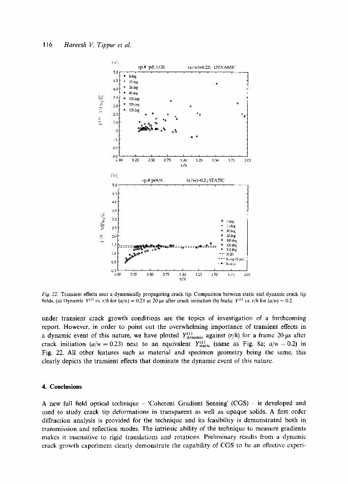
Fig. 22. Transient effects near a dynamically propagating crack tip: Comparison between static and dynamic crack tip fields. (a) Dynamic Y") vs. r/h for (a/w) = 0.23 at 20 Its after crack initiation (b) Static yill vs. r/h for (a/w) = 0.2.

under transient crack growth conditions are the topics of investigation of a forthcoming report. However, in order to point out the overwhelming importance of transient effects in a dynamic event of this nature, we have plotted v(1) against (r/h) for a frame 20 ~ts after * d y n a m i c

crack initiation (a/w = 0.23) next to an equivalent Ystatie(1) (same as Fig. 8a; a/w = 0.2) in Fig. 22. All other features such as material and specimen geometry being the same, this clearly depicts the transient effects that dominate the dynamic event of this nature.

4. Conclusions

A new full field optical technique 'Coherent Gradient Sensing' (CGS) - is developed and used to study crack tip deformations in transparent as well as opaque solids. A first order diffraction analysis is provided for the technique and its feasibility is demonstrated both in transmission and reflection modes. The intrinsic ability of the technique to measure gradients makes it insensitive to rigid translations and rotations. Preliminary results from a dynamic crack growth experiment clearly demonstrate the capability of CGS to be an effective experi-


mental alternative to other optical methods used in dynamic fracture studies such as photoelasticity and caustics. Notably, it is a full field technique which works with optically isotropic materials. It also has a potential for application to study dynamic fracture of metals.

The static fringe patterns obtained from the experiments are analyzed in regions outside the 3-D zone. For geometries where the region outside the 3-D zone is K-dominant, the fringes provide an accurate value of 2-D stress intensity factor. For geometries where the region outside the 3-D zone is not K-dominant, Williams' expansion is used in conjunction with a least squares procedure to obtain the stress intensity factor.

Acknowledgments

Support of ONR through Contracts N00014-85-K-0596 and N00014-90-J-1340 and of NSF through the Presidential Young Investigator Award (Grant MSM-84-51204) to A JR is gratefully acknowledged.

References

1. F.P. Chiang, in Manual of Experimental Stress Analysis Techniques, A.S. Kobayashi (ed.), SESA 3rd Edition (1978). 2. I. Glat and O. Kafri, Optics and Lasers in Engineering 8 (1988) 277-320. 3. F.P. Chiang and R.M. Juang, Applied Optics 15 (1976) 2199-2204. 4. K. Patorski, Journal of Optical Society of America - A, 3 (1986) 1862-1868. 5. Y.Y. Hung and A.J. Durelli, Journal of Strain Analysis 14(3) (1979) 81-88. 6. Y.J. Chao, M.A. Sutton and C.E. Taylor, in Proceedings of the Society of Experimental Stress Analysis, B.E. Rossi

(ed.) 38 (1982). 7. R.J. Sanford and J.W. Dally, Journal of Engineering Fracture Mechanics 11 (1979) 621-633. 8. R. Chona, G.R. Irwin and R.J. Sanford, ASTM STP 791, 1 (1983) 3-13. 9. H. Nigam and A. Shukla, Experimental Mechanics 3 (1988) 123-135.

10. P.S Theocaris, in Mechanics of Fracture, Vol. VII, G.C. Sih (ed.), Sijthoff and Noordhoff (1981). 1 l. J. Beinert and J.F. Kalthoff, Mechanics of Fracture, Vol. VII, G.C. Sih (ed.), Sijthoff and Noordhoff (1981). 12. A.J. Rosakis and A.T. Zehnder, Journal of Elasticity 4 (1985) 347-367. 13. K. Ravi-Chandar and W.G. Knauss, International Journal of Fracture 25 (1984) 247-262. 14. A.J. Rosakis and K. Ravi-Chandar, International Journal of Solids and Structures 22(2) (1986) 121-134. 15. F.P. Chiang and T.V. Hareesh, International Journal of Fracture 36 (1988) 243-257. 16. B.S.J. Kang, A.S. Kobayashi and D. Post, Experimental Mechanics 27(3) (1987) 243-245. 17. W. Yang and L.B. Freund, International Journal of Solids and Structures 21(9) (1985) 977-994. 18. T. Nakamura and D.M. Parks, Journal of Applied Mechanics 55(4) (1988) 805-813. 19. R. Narasimhan, A.T. Zehnder and A.J. Rosakis, Proceedings of Symposium on Analytical, Numerical and Experimen-

tal Aspects of Three Dimensional Fracture Processes, AJ. Rosakis, K. Ravi-Chandar and Y. Rajapakse (eds.) ASME Annual Meeting, Berkeley, CA, June (1988).

20. I.D. Parsons, J.F. Hall and A.J. Rosakis, Proceedings of 20th Midwestern Mechanics Conference, West Lafayette, Indiana, August (1987).

21. S. Krishnaswamy, A.J. Rosakis and G. Ravichandran, Caltech Report SM88-21 (1988) (submitted to Journal of Applied Mechanics).

22. H.V. Tippur, S. Krishnaswamy and AJ. Rosakis, International Journal of Fracture 48 (1991) 193-204. 23. M.L. Williams, Journal of Applied Mechanics 24 (1959) 109-114. 24. D.P. Rooke and D.J. Cartwright, Compendium of Stress Intensity Factors, Her Majesty's Stationery Office (1975).

optical mapping of crack tip deformations using the...

Documents