optimal acquisition and sorting policies for
TRANSCRIPT

University of Massachusetts Amherst University of Massachusetts Amherst
ScholarWorks@UMass Amherst ScholarWorks@UMass Amherst
Masters Theses 1911 - February 2014
2009
Optimal Acquisition and Sorting Policies for Remanufacturing Optimal Acquisition and Sorting Policies for Remanufacturing
over single and Multiple Periods over single and Multiple Periods
Yihao Lu University of Massachusetts Amherst
Follow this and additional works at: https://scholarworks.umass.edu/theses
Lu, Yihao, "Optimal Acquisition and Sorting Policies for Remanufacturing over single and Multiple Periods" (2009). Masters Theses 1911 - February 2014. 240. Retrieved from https://scholarworks.umass.edu/theses/240
This thesis is brought to you for free and open access by ScholarWorks@UMass Amherst. It has been accepted for inclusion in Masters Theses 1911 - February 2014 by an authorized administrator of ScholarWorks@UMass Amherst. For more information, please contact [email protected].

OPTIMAL ACQUISITION AND SORTING POLICIESFOR REMANUFACTURING OVER SINGLE AND
MULTIPLE PERIODS
A Thesis Presented
by
YIHAO LU
Submitted to the Graduate School of theUniversity of Massachusetts Amherst in partial fulfillment
of the requirements for the degree of
MASTER OF SCIENCE IN INDUSTRIAL ENGINEERING AND OPERATIONSRESEARCH
February 2009
Department of Mechanical and Industrial Engineering

OPTIMAL ACQUISITION AND SORTING POLICIESFOR REMANUFACTURING OVER SINGLE AND
MULTIPLE PERIODS
A Thesis Presented
by
YIHAO LU
Approved as to style and content by:
Ana Muriel, Chair
Erin Baker, Member
Thomas Brashear-Alejandro, Member
Mario Rotea, Department HeadDepartment of Mechanical and Industrial En-gineering

To my parents, Yuya and Xiaodi.

ACKNOWLEDGMENTS
I would like to thank my advisor, Professor Ana Murial, for her many years of
thoughtful, patient guidance and support. Thanks are also due to the members of
my committee, Professor Erin Baker and Professor Thomas Brashear-Alejandro, for
their helpful comments and suggestions on all stages of this thesis.
I wish to express my appreciation to all those whose support and friendship helped
me to stay focused on my work and provided me with the encouragement to continue
when the going got tough.
iv

TABLE OF CONTENTS
Page
ACKNOWLEDGMENTS . . . . . . . . . . . . . . . . . . . . . . . . . . . . . . . . . . . . . . . . . . . . . iv
LIST OF TABLES . . . . . . . . . . . . . . . . . . . . . . . . . . . . . . . . . . . . . . . . . . . . . . . . . . . vii
LIST OF FIGURES . . . . . . . . . . . . . . . . . . . . . . . . . . . . . . . . . . . . . . . . . . . . . . . . . .viii
CHAPTER
1. INTRODUCTION . . . . . . . . . . . . . . . . . . . . . . . . . . . . . . . . . . . . . . . . . . . . . . . . . 1
1.1 Remanufacturing . . . . . . . . . . . . . . . . . . . . . . . . . . . . . . . . . . . . . . . . . . . . . . . . . 31.2 Challenges in Remanufacturing . . . . . . . . . . . . . . . . . . . . . . . . . . . . . . . . . . . . . 61.3 Product Acquisition Management and Sorting Policies . . . . . . . . . . . . . . . . . 81.4 Research Objectives and Outline . . . . . . . . . . . . . . . . . . . . . . . . . . . . . . . . . . . 11
2. RELATED LITERATURE . . . . . . . . . . . . . . . . . . . . . . . . . . . . . . . . . . . . . . . . 13
3. SINGLE-PERIOD OPTIMAL ACQUISITION AND SORTINGPOLICIES . . . . . . . . . . . . . . . . . . . . . . . . . . . . . . . . . . . . . . . . . . . . . . . . . . . . . 16
3.1 Model Assumptions . . . . . . . . . . . . . . . . . . . . . . . . . . . . . . . . . . . . . . . . . . . . . . 163.2 Model Description . . . . . . . . . . . . . . . . . . . . . . . . . . . . . . . . . . . . . . . . . . . . . . . 18
3.2.1 Notation . . . . . . . . . . . . . . . . . . . . . . . . . . . . . . . . . . . . . . . . . . . . . . . . . 183.2.2 Buy-back Cost . . . . . . . . . . . . . . . . . . . . . . . . . . . . . . . . . . . . . . . . . . . . 193.2.3 Remanufacturing Cost . . . . . . . . . . . . . . . . . . . . . . . . . . . . . . . . . . . . . 19
3.3 Optimization Problem . . . . . . . . . . . . . . . . . . . . . . . . . . . . . . . . . . . . . . . . . . . . 203.4 Model Analysis . . . . . . . . . . . . . . . . . . . . . . . . . . . . . . . . . . . . . . . . . . . . . . . . . . 23
3.4.1 Linear Acquisition Cost . . . . . . . . . . . . . . . . . . . . . . . . . . . . . . . . . . . . 233.4.2 Piecewise Linear Cost . . . . . . . . . . . . . . . . . . . . . . . . . . . . . . . . . . . . . . 24
3.5 Numerical Study . . . . . . . . . . . . . . . . . . . . . . . . . . . . . . . . . . . . . . . . . . . . . . . . 27
v

4. MULTI-PERIOD OPTIMAL ACQUISITION AND SORTINGPOLICIES . . . . . . . . . . . . . . . . . . . . . . . . . . . . . . . . . . . . . . . . . . . . . . . . . . . . . 32
4.1 Model Assumptions . . . . . . . . . . . . . . . . . . . . . . . . . . . . . . . . . . . . . . . . . . . . . . 324.2 Model Description . . . . . . . . . . . . . . . . . . . . . . . . . . . . . . . . . . . . . . . . . . . . . . . 34
4.2.1 Notation . . . . . . . . . . . . . . . . . . . . . . . . . . . . . . . . . . . . . . . . . . . . . . . . . 344.2.2 acquisition Cost . . . . . . . . . . . . . . . . . . . . . . . . . . . . . . . . . . . . . . . . . . . 364.2.3 Remanufacturing Cost . . . . . . . . . . . . . . . . . . . . . . . . . . . . . . . . . . . . . 374.2.4 Inventory Cost . . . . . . . . . . . . . . . . . . . . . . . . . . . . . . . . . . . . . . . . . . . . 394.2.5 Inventory Constraints . . . . . . . . . . . . . . . . . . . . . . . . . . . . . . . . . . . . . . 39
4.3 Multi-Period Optimization Problem . . . . . . . . . . . . . . . . . . . . . . . . . . . . . . . . 404.4 Convexity of the Cost Function . . . . . . . . . . . . . . . . . . . . . . . . . . . . . . . . . . . . 424.5 Linear Acquisition Cost Without Core Holding . . . . . . . . . . . . . . . . . . . . . . 48
4.5.1 Special Cases . . . . . . . . . . . . . . . . . . . . . . . . . . . . . . . . . . . . . . . . . . . . . 504.5.2 General Cases . . . . . . . . . . . . . . . . . . . . . . . . . . . . . . . . . . . . . . . . . . . . 50
4.5.2.1 Solution for a Single Set . . . . . . . . . . . . . . . . . . . . . . . . . . . 524.5.2.2 Solution for General Cases . . . . . . . . . . . . . . . . . . . . . . . . . 544.5.2.3 Quantity-Independent Optimal Yield . . . . . . . . . . . . . . . . 55
4.6 Linear Acquisition Cost With Core Holding . . . . . . . . . . . . . . . . . . . . . . . . . 56
4.6.1 A Simple Case . . . . . . . . . . . . . . . . . . . . . . . . . . . . . . . . . . . . . . . . . . . . 574.6.2 Linear Acquisition Cost With Core Holding . . . . . . . . . . . . . . . . . . . 59
5. CONCLUSIONS . . . . . . . . . . . . . . . . . . . . . . . . . . . . . . . . . . . . . . . . . . . . . . . . . . 61
BIBLIOGRAPHY . . . . . . . . . . . . . . . . . . . . . . . . . . . . . . . . . . . . . . . . . . . . . . . . . . . 64
vi

LIST OF TABLES
Table Page
1.1 Responsibilities of PrAM. Adapted from Guide 2000 [23] . . . . . . . . . . . . . . 10
vii

LIST OF FIGURES
Figure Page
1.1 Structure of a remanufacturing facility. Adapted from Guide 2000[22] . . . . . . . . . . . . . . . . . . . . . . . . . . . . . . . . . . . . . . . . . . . . . . . . . . . . . . . . . . 5
3.1 Remanufacturing Flowchart . . . . . . . . . . . . . . . . . . . . . . . . . . . . . . . . . . . . . . . 17
3.2 Acquisition cost vs. acquired amount . . . . . . . . . . . . . . . . . . . . . . . . . . . . . . . 19
3.3 Remanufacturing cost vs. remanufacturing yield . . . . . . . . . . . . . . . . . . . . . 20
3.4 Remanufacturing cost vs. yield . . . . . . . . . . . . . . . . . . . . . . . . . . . . . . . . . . . . 21
3.5 Piecewise acquisition cost . . . . . . . . . . . . . . . . . . . . . . . . . . . . . . . . . . . . . . . . . 25
3.6 Acquisition cost vs. acquired quantity, piece-wise linear . . . . . . . . . . . . . . . 28
3.7 Distribution of Γ(5, 2) . . . . . . . . . . . . . . . . . . . . . . . . . . . . . . . . . . . . . . . . . . . . 29
3.8 Optimal yield vs. demand . . . . . . . . . . . . . . . . . . . . . . . . . . . . . . . . . . . . . . . . 29
3.9 Total cost vs. demand . . . . . . . . . . . . . . . . . . . . . . . . . . . . . . . . . . . . . . . . . . . . 30
3.10 Total cost, optimal yield vs. optimal acquisition . . . . . . . . . . . . . . . . . . . . . 31
4.1 Model Time Line . . . . . . . . . . . . . . . . . . . . . . . . . . . . . . . . . . . . . . . . . . . . . . . . 33
4.2 Acquisition cost for different periods. . . . . . . . . . . . . . . . . . . . . . . . . . . . . . . . 36
4.3 Remanufacturing cost for different periods. . . . . . . . . . . . . . . . . . . . . . . . . . . 37
4.4 Remanufacturing cost - Yield for different periods. . . . . . . . . . . . . . . . . . . . 38
4.5 General Problem with Linear Acquisition Cost . . . . . . . . . . . . . . . . . . . . . . 51
4.6 General Solution with Linear Acquisition Cost . . . . . . . . . . . . . . . . . . . . . . . 52
viii

4.7 Base of General Solution for one Set . . . . . . . . . . . . . . . . . . . . . . . . . . . . . . . 52
4.8 Base of General Solution . . . . . . . . . . . . . . . . . . . . . . . . . . . . . . . . . . . . . . . . . 54
ix

CHAPTER 1
INTRODUCTION
The drastic development in industry and increase in population during the past
centuries has caused the natural resources depletion, wide spread pollution and in-
crease on land for food production. As a result, many countries and environmental
protection agencies enforce stricter regulations (such as the European Union’s WEEE
directive 2003) for the companies to assume responsibilities for the disposal of their
products as well as reduce their waste.
Those strict government regulations, along with the increasing number of en-
vironmentally conscious consumers and the progress in ecological design have been
bringing the handling of used products to the forefront of business priorities ([7, 8, 26,
28, 37, 41]). Consequently, manufacturers are encouraged to take interest in product
recovery and the after-sale market.
Although the remanufacturing industry emerged under these environmental con-
cerns, it is becoming a profitable business model ([14, 16, 21, 29, 30, 31, 32]). More-
over, in contrast to the common belief that the remanufactured products may can-
nibalize the market of new products, researchers have found that remanufacturing
may increase market share under the right circumstances ([20, 31, 36]). Therefore,
remanufacturing industry, along with its high labor-intensity ([14, 30]) as well as the
contribution to energy and material conservation, provides economic, environmental
and social benefits.
According to Hauser and Lund [33], the size of the remanufacturing sector in
the United States is $53 billion, with over 70,000 firms and 480,000 employees. The
1

average profit margin is estimated to exceed 20% [43]. Throughout the world, the
total size of remanufacturing has reached more than $100 billion. Many independent
businesses have emerged to exploit the potential profitable remanufacturing oppor-
tunities [52] such that today the Original Equipment Manufacturers (OEM) only
account for five percent of the remanufacturing industry’s total sales. Today, there
are three sectors in this industry: the OEM and their first tier suppliers, the OEMs’
subcontractors, and independent remanufacturers [46].
In this thesis, we study one major problem in remanufacturing, namely, sorting
policies that specify which returned items should be remanufactured and which should
be scrapped. We examine a remanufacturer who acquires used products from third
party brokers or directly from the market in multiple periods. Due to the high
variability of those acquired items’ condition, the remanufacturer has to make three
related decisions: (1) how many used items to acquire; (2) how selective to be during
the sorting process and (3) how many remanufactured products to be kept in inventory
for future demands. While the deterministic demands are always satisfied without
backlogging, postponing acquiring may lead to a lower per-unit acquiring cost and
a higher per-unit remanufacturing cost, as we take the condition deterioration into
account. Moreover, as more items are acquired, and hence a higher per-unit acquiring
cost, for a given demand, the remanufacturer can be more selective when sorting, and
thus a lower per-unit remanufacturing cost. We study the trade-off among these
factors and derive optimal acquisition, remanufacturing and inventory quantity in
the presence of product condition variability for a remanufacturer facing deterministic
demand. In the following sections, we first review the definition and applications of
remanufacturing. Two cases, Fuji Xerox and Kodak, are studied. In Section 1.2, we
review the challenges in remanufacturing research given by Guide [22], followed by
an introduction on product acquisition management and sorting policies, which is the
2

focus of our work. At the end of this chapter, we state our research objectives and
introduce the outline of this thesis.
1.1. Remanufacturing
According to The Remanufacturing Institute (http://www.reman.org/faq.htm), a
product is defined as remanufactured if:
• Its primary components come from a used product.
• The used product is dismantled to the extent necessary to determine the conditionof its components.
• The used product’s components are thoroughly cleaned and made free from rust andcorrosion, if needed.
• All missing, defective, broken or substantially worn parts are either restored to sound,functionally good condition, or they are replaced with new, remanufactured, or sound,functionally good used parts.
• To put the product in sound working condition, such matching, rewinding, refinishingor other operations are performed as necessary.
• The product is reassembled and a determination is made that it will operate like asimilar new product.
In this thesis, we apply this definition and use the term “remanufacturing” inter-
changeably with “refurbishing” and “reconditioning”.
However, not all products are suitable for remanufacturing. It depends on the
availability of returned cores, the product’s life span and the technical progress re-
garding new versus remanufactured products [48]. Usually, before the remanufactur-
ing decision is made, a firm needs to determine whether such remanufacturing can be
realized with current technologies in mass production scale. Currently, auto-parts,
tires, furniture, laser toner cartridges, and computers and electrical equipment are
among the appropriate products for remanufacturing. Other typical remanufactured
products include mattresses and carpets.
Fuji Xerox and Kodak are good examples of firms that are successfully supple-
menting their business with remanufacturing capability.
3

Fuji Xerox
Fuji Xerox, a joint venture between Japan’s Fuji Photo Film Co Ltd and the US
Rank Xerox Limited from 1962, is one of the world’s leading manufacturers of office
equipment. By the end of 2006, this joint venture had 40,295 employees and generated
1,163.3 billion Japanese Yen revenue around the world (www.fujixerox.com).
Fuji Xerox started its business by renting its products to customers and then
moved on to selling and leasing the products. Through its early practice in serving
contracts with repairing or replacing consumables, the firm developed its remanufac-
turing capability and its closed loop supply chain. In 2000, Fuji Xerox became the
first to achieve zero landfill of used products in Japan. It also built its remanufac-
turing facilities in Sydney in 1993, where valuable components had been considered
waste even with minor defects. It is believed the new operation even improves the
performance of the products [5].
In 2004 alone, Fuji Xerox diverted 128 million pounds of material from entering
landfills through part recycling and reuse. From reuse alone, it saved approximately
11 million therms of energy and around 70,000 machines were remanufactured. At
the same time, Fuji Xerox remains one of the most profitable firms in its industry.
Kodak
Kodak introduced its single-use cameras in 1987 to capture the market of occa-
sional users. After taking the pictures, the cameras had to be returned to a photo-
finisher for printing. This is the reason such cameras are called “disposables” or
“throwaways”.
The product had an outstanding picture quality and received an immediate suc-
cess among customers who were looking for budget picture taking solutions. However,
some environmental groups raised concerns about the potential for a significant in-
crease in the amount of solid waste generated.
4

( )V.D.R. Guide Jr.rJournal of Operations Management 18 2000 467–483470
research in specific production planning and controlactivities.
A part of the purpose of this research is toidentify areas that have not been fully addressed, orthat have not been investigated at all. In the researchissues section, the current research needs are recon-ciled with previous research issues. A shortcomingof the existing literature is that no research developsintegrated systems for planning and control of ope-rational activities, and much of the research failsto consider the interactions between complicatingcharacteristics. In Section 5, we present empiricalevidence that supports each the complicating charac-teristics, and show how production planning andcontrol activities are specifically affected.
Given the high profitability, growing number oflegislative initiatives and growing consumer aware-ness, the time is right for the formal development ofsystems for managing remanufacturing processes. Atpresent, these systems exist on a number of scales,ranging from facilities remanufacturing brake shoesto facilities remanufacturing entire aircraft. However,they all lack an integrated body of knowledge ofhow to design, manage and control their operations.
Remanufacturing firms have a more complex shopŽstructure to plan, control and manage Guide and
.Srivastava, 1998; Guide et al., 1997b . This addi-tional complexity is a function of stochastic product
returns, disassembly operations, and highly variablematerial processing requirements. We discuss theseand other factors in detail in the following sections.A typical remanufacturing facility consists of threedistinct sub-systems: disassembly, processing, andreassembly, all of which must be carefully coordi-
Ž .nated see Fig. 1 . Disassembly is the first step inremanufacturing operations and provides the partsand components for processing. Disassembly is alsoan important information gateway, as discussed inthe following section. Remanufacturing operationslayouts are most commonly in a job-shop form be-cause of the use of general-purpose equipment, and
Ž .the need for flexibility Nasr et al. 1998 . Less thanŽ .one-fifth 17.4% of remanufacturers report using
specialized CNC equipment or manufacturing cellsŽ .Nasr et al., 1998 . This may be, in part, from thediversity in products remanufactured and the low
Ž .production volumes. Nasr et al. 1998 suspect thatthe low level of technology is because of a lack ofspecialized production and control systems. Re-assembly is the final stage in a remanufacturingsystem. Because of the high variability of remanufac-turing processing times and the large number of
Žoptions for parts new, remanufactured and substi-.tutable , the task of scheduling is more complex and
more likely to be done with simple rule-of-thumbtechniques. Remanufacturers may carry a variety of
Fig. 1. Elements of a remanufacturing shop.
Figure 1.1. Structure of a remanufacturing facility. Adapted from Guide 2000 [22]
Therefore, Kodak began to redesign its single-use cameras in 1990 [24], which
led to a remarkable global recycling and re-use program. The redesign facilitated
recycling and re-use of parts. Over the years, the Kodak cameras have been so well
designed that up to 90% of the product is remanufacturable. The remaining parts
can be recycled such that virtually no part is sent to a landfill.
Today, the recycling rate for one-time use cameras in US is greater than 75%, the
highest among all consumer products in this country. More than 90% of the parts of
a new camera sold orginates from remanufacturing. The number of Kodak one-time-
use cameras recycled is now more than 800 million. When considering competitors
cameras that are also collected through Kodak, the total number of recycled exceeds
one billion cameras.
While each firm may face its specific problem in remanufacturing, several common
challenges have been identified by prior research.
5

1.2. Challenges in Remanufacturing
Guide divides the remanufacturing facilities into three sub-systems: disassembly,
processing, and reassembly (see Figure 1.1). Given its high dependence on the stream
of returned products, remanufacturing is quite different from traditional manufactur-
ing. In his well cited article regarding potential research topics, Guide lists seven
characteristics which complicate the production planning and control activities in
remanufacturing [22]. They are:
1. The uncertain timing and quantity of returns. The uncertainty of a product’s life
cycle and the change of technology and market preference cause the variability
of timing and amount of available cores. This issue is made worse as, in the
early life phase when the remanufactured product may have more market share,
there are fewer cores on the market, compared to the late phases. Firms are
trying to attack this problem by some form of core deposit system, i.e., trying
to generate a core when a remanufactured product is sold. Trade-in, charging
a premium if no core is returned, and leasing instead of selling are among the
examples. However, such practices have not solved the built-in uncertainty and
remanufacturing firms still report that core inventories account for one-third of
the inventory carried [43].
2. The need to balance returns with demands. Meeting demands with supply
is important to profit-maximizing firms and has been studied extensively in
the traditional production planning literature. It is well known that both lost
sales and excessive inventory cut profit. However, in remanufacturing, supply
and demand have a more complicated relationship; that is, they are coupled
together. The excess or scarcity of cores depends on the demand met previously.
3. The disassembly of returned products. Disassembly, as the first step in the
operations, involves inspecting the product and retrieving the components for
6

further processing. Products are disassembled to the part level, assessed as
to their remanufacturability and acceptable parts are then routed to further
processing. Parts that can not meet minimum remanufacturing standards may
be used for spares or sold for scrap value. Moreover, products designed for
easy assembly may not be well designed for disassembly. These factors in dis-
assembly cause high variability in disassembly time and thus the lead time in
remanufactured products. In fact, Guide reports the coefficients of variance
for disassembly time can be as high as 5.0. This hurts the competitiveness of
remanufacturers.
4. The uncertainty in materials recovered from returned items. Material Recover-
ability Rate, or MRR, is used to measure the recovery uncertainty [25]. MRR is
applied to determine batch size for purchasing and manufacturing. The majority
of firms report to estimate the MRR by simple average, but some sophisticated
regressive models have also been used. Most common inputs to the MRR es-
timation model is historical data, although procurer’s subjective estimation is
also used sometimes. To decide the purchase batch size, dynamic lot sizing
techniques are most commonly used. The concerns with the purchasing process
includes long purchase lead time, sole suppliers for some part, uncertainty in
demand and small purchase orders.
5. The requirement for a reverse logistics network. A reverse network is needed
to collect the returns from the end user to the remanufacturer. For high value
cores, trade-in systems, which connect the customers directly with the firms,
is a common practice. However, for low value items, alternatives are required
to motivate the returns. The three most used methods are core brokers, third
party agencies and seed stock.
7

6. The complication of material matching restrictions. Some remanufacturing
practices are complicated by special material matching restrictions. For ex-
ample, in after-market aviation maintenance industry, remanufacturing orders
are mostly driven by customers who retain the ownership of the product and
require the same unit returned. This obliges the coordination between disas-
sembly, reprocessing and assembly operations. Concerns raised here include
short planning horizons and poor visibility for replacement parts, which are
familiar to make-to-order production systems. The material matching restric-
tions may also pose a high burden on scheduling and information systems. For
products with complicated structures, tens of thousands of parts may need to
be numbered, tagged and tracked.
7. The problems of stochastic routings for materials for remanufacturing opera-
tions and highly variable processing times. Given the variable condition of the
returns, each item may have its unique requirement of processing steps. For ex-
ample, while all the returns may have to go through the cleaning process, other
routings may be probabilistic and highly dependent on the age and condition
of the part. This causes difficulties in estimating flow time and planning both
machine and labor resources. Determining machine structure and setup times
also become complicated. This characteristic is claimed to be the single most
complicating factor of lot sizing decisions and scheduling.
There are several activities remanufacturers are practicing to handle the issues
listed above. In the next section, we review these activities and our focus is on
Production Acquisition Management, the major interest of this thesis.
1.3. Product Acquisition Management and Sorting Policies
There are three primary groups of activities in remanufacturing [31], namely,
Production Returns Management (PRM), Remanufacturing Operational Issues and
8
Remanufactured Products Market Development, and each of them has seen exten-
sive work during the years. PRM, which includes Product Acquisition Management
(PrAM), studies the issues related to the timing, quantity, and quality of returned
products ([3, 49]). Remanufacturing Operational Issues focus on reverse logistics,
testing, sorting and disposing, product disassembly and remanufacturing processes
([2, 19, 44]). The Remanufactured Products Market Development includes remanu-
factured products marketing strategies and channels, market competition as well as
cannibalization ([6, 9, 38, 51] ). In this paper, our major work focuses on PRM, or
to be more specific, PrAM.
Among the challenges listed in the last section, PrAM mainly helps to handle (1)
uncertainty in timing and quantity of returns; (2) balancing returns with demands; (4)
material recovery uncertainty; (5) reverse logistics and (6) customer-required returns.
In Guide et al. 2000 [23], the authors report six responsibilities for PrAM activities:
1. Core acquisition. While core acquisition is mostly a purchasing function, inputs
from operations are necessary to develop criteria in evaluating the condition of
the cores acquired from various sources. These criteria may include quality,
cost, and quantity.
2. Forecasting core availability. Core availability is critical to production planning
in remanufacturing. Factors affecting availability include the product life-cycle
position, rate of technological change and economic conditions. Given the cou-
pling nature of core supply and previous demand, forecasting involves the co-
operation of purchasing, operations and marketing. A better forecast will save
inventory holding or lost sales.
3. Synchronizing return rates with demand rates. As shown in the last section, in
remanufacturing, both demand and core supply need to be forecast. This calls
for the cooperation between purchasing and marketing to match the return
9

rate with demand rate for remanufactured products. This problem is further
complicated by the uncertainty in the material recovery rate, which in turn calls
the inputs from operations.
4. Coordinating replacement materials. New parts and components are needed to
replace materials that are technologically or economically unrecoverable. Due
to the variability in quality of the returns, coordination between purchasing and
operations on an on-going basis is often required.
5. Resource planning. Uncertainty in quality, quantity and time of the returns
make it difficult to allocate and schedule machine and labor. Therefore, PrAM
is also responsible for the inputs to capacity planning for remanufacturers.
6. Reducing the uncertainties in returns. The responsibilities listed above help
to reduce the associated costs at an operational level. However, firms need to
develop long term strategies to reduce the inherited uncertainty rooted in the
return process. Core deposits, leasing and trade-ins are potential alternatives
currently being studied.
These six responsibilities all involve firm-wise cooperation, because of the cou-
pled (looping) nature of remanufacturing. Guide et al. 2000 [23] summarizes the
involvement with a table (Table 1.1).
Table 1.1. Responsibilities of PrAM. Adapted from Guide 2000 [23]
Responsibility Operations Purchasing Marketing(1) Core acquisition
√ √
(2) Forecasting core availability√ √
(3) Synchronizing returns with demands√ √ √
(4) Coordinating materials replacement√ √ √
(5) Resource planning√ √
(6) Reducing uncertainty in returns√ √
10

The acquisition/sorting policy refers to the operational decision on which returned
products should be remanufactured and which should be scrapped [18]. Not all returns
may be remanufactured due to the technological or economical constraints. Items that
cannot be recovered have to be scrapped; for the sake of simplicity, we do not consider
other alternatives, such as recycling. Therefore, to satisfy certain demand, firms need
to acquire more cores than the projected demand. In general, a less stringent sorting
will generate more available cores and thus less returns are needed to be acquired.
This lowers the total acquisition cost. However, this lower selectivity may require
sophisticated recovery technologies and command a higher per unit recovery cost.
The interaction between these two factors will drive the optimal acquisition/sorting
policy in any single period.
1.4. Research Objectives and Outline
In this thesis, we extend the earlier work of Galbreth and Blackburn [18] to a
multi-period model. The work of [18] will be covered in detail in Chapter 3. As
in their paper, we assume the per unit remanufacturing costs are convex increasing
functions in quality, to capture the fact that the remanufacturing cost increases as
quality decreases.
For many consumer goods, the longer the product has been used, the worse its
condition and thus, the lower its buy-back cost. We capture this effect by assuming
the acquisition cost decreases in time while the remanufacturing cost increases in
time.
The remanufacturer follows a “make from stock” model; i.e., products are acquired
and available as needed to meet remanufacturing needs. A typical example is cellular
phone industry where used products are purchased from brokers as needed to fulfill
specific demands.
11

The remainder of this thesis is organized as follows. In Chapter 2, we will review
the literature most closely related to our work. In Chapter 3, after we introduce the
model developed by Galbreth and Blackburn, we extend their work to a more general
case. The study and results of multi-period problem are presented in Chapter 4,
where we first introduce the multi-period model, show the convexity of the general
objective function and then study a special case – linear acquisition cost. We also
extend our work to relax the no-core-holding constraint at the end of Chapter 4. We
conclude with the outline and prospectus of future study in Chapter 5.
12

CHAPTER 2
RELATED LITERATURE
It is well acknowledged that variability in supply quality, quantity and timing poses
a huge challenge to remanufacturing ([1, 22, 23, 47]) and extensive literature can be
found in the study of such uncertainty. For example, Toktay et al. [50] use a queuing
network model to study the uncertainty in processing time. Simulation models are
also developed. Humphrey et al. [34] simulate the variable repair requirements in
a reverse logistics network. Guide et al. [27] also incorporate stochastic processing
time into their simulation model in an evaluation of various order release strategies.
Many aspects of the variability in quality of the returns have been studied. Fer-
guson and Toktay [13] assume the variable cost of collection increases in the quantity
of the products collected/processed in a single period and use this model to study the
cannibalism between the new and remanufactured products.
In his Remanufacturing Aggregate Production Planning (RAPP) model, Jayara-
man [35] proposes to capture the variability of returned products’ condition through
a discrete distribution of nominal quality, which is expressed as an n-dimensional
vector. RAPP is a unit cost minimizing linear programming model, in which the
yield is assumed to be a constant within each quality category. Given the linearity
nature of his model, costs are all assumed proportional to the total number. Bakal
and Akcali [4] extend this work, still in a single-period setting, to a problem where
both the quantity and quality of the returned products depends on the acquisition
price offered. Moreover, the remanufacturer has control over the demand for the final
products by pricing.
13

In Ferrer [15], it is found the information of yield is generally quite valuable under
infinite horizon using Markov Decision Processes. Ketzenberg et al. [39] further
extend it to consider uncertainty in demand, returns along with yield.
Guide [22] identifies the need to estimate used product condition to determine
the appropriate disposition, which is an important step in determining the optimal
recovery action. Therefore, an inspection decision is a necessity. However, the sorting
policies in remanufacturing have received limited scrutiny in the literature. Guide
and Wassenhove [30] study the optimal acquisition policies and pricing, where they
assume products are acquired from third-party brokers with quality categories and
known remanufacturing cost.
The work most closely related to ours is in Ferguson et al.[11, 12], and Galbreth
and Blackburn [18]. In [11], the authors study a multi-period production planning
problem and assume the number of returns in each period is known. Returns are
tested and categorized into a finite number of nominal quality categories, such as,
good, better and best. For each category, the remanufacturing cost is assumed to
be a constant such that the cost structure is a piecewise linear convex curve in the
total quantity of products remanufactured. This work is further extended to include
uncertainty in quality levels with stochastic programming in [11]. The model is solved
numerically and, given its nature of exponential increase in the number of outcomes,
its computational complexity of this model grows very fast.
In Galbreth and Blackburn [18], the authors examine the single period case in
which a remanufacturer acquires unsorted products from third party brokers in the
presence of product condition variability. As more used items are acquired for a
given demand, the remanufacturer can be more selective when sorting. Two related
decisions are made: how many used items to acquire, and how selective to be during
the sorting process while the fixed demand is always satisfied. The existence of a single
optimal acquisition and sorting policy with a simple structure is proved. The authors
14

also show that the policy of selectivity is independent of the production amount
when acquisition costs are linear. In [17], those authors extend it to study stochastic
yield. They find that the deterministic yield is often a reasonable approximation to
its stochastic counterpart.
Our major objective in this thesis is to extend the single period model in Galbreth
and Blackburn [18]. While these authors have studied the single period problem when
acquisition cost is linear, in the next chapter, we will reproduce their work and then
continue to study when the acquisition cost is piecewise linear convex instead.
15
CHAPTER 3
SINGLE-PERIOD OPTIMAL ACQUISITION ANDSORTING POLICIES
In this chapter, we formulate the single-period model and then reproduce the
work by Galbreth and Blackburn [18] when the acquisition cost is linear. We will
then study the case when the acquisition cost is a piecewise linear convex function.
3.1. Model Assumptions
Many electronic products have relatively short life cycles. For example, fast grow-
ing communication techniques have been making the cell phone devices’ life much
shorter than their functional life. For these products, a single-period model is rea-
sonable given that future demand is not guaranteed.
As mentioned in Chapter 1, to simplify our model, we assume the returned cores
are either remanufactured or scrapped. No other alternative such as raw material
recycling is considered. The extension to include those alternatives should not change
the sorting and acquisition decision if scrapping cost is introduced into the model,
as they may be absorbed into the remanufacturing yield curve. Figure 3.1 shows the
flowchart of the remanufacturing processes. At the beginning of the planning period,
the firm needs to determine the total amount (p) to acquire from the market or dealers.
Given that it is not economically feasible to remanufacture low quality products, the
firm needs to decide, among the acquired, r items to be remanufactured and the rest
p−r to be scrapped (p ≥ r). Perfect testing, which means that at the time of sorting,
the corresponding remanufacturing cost is known based on the observed condition,
16
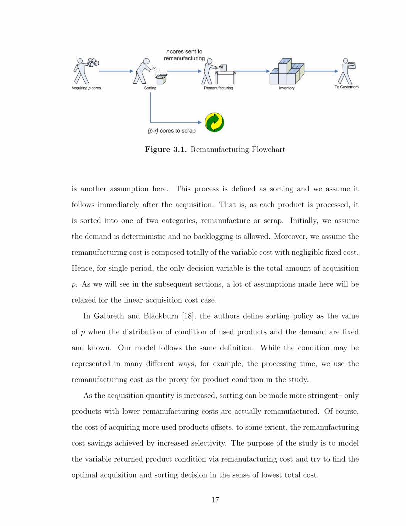
Figure 3.1. Remanufacturing Flowchart
is another assumption here. This process is defined as sorting and we assume it
follows immediately after the acquisition. That is, as each product is processed, it
is sorted into one of two categories, remanufacture or scrap. Initially, we assume
the demand is deterministic and no backlogging is allowed. Moreover, we assume the
remanufacturing cost is composed totally of the variable cost with negligible fixed cost.
Hence, for single period, the only decision variable is the total amount of acquisition
p. As we will see in the subsequent sections, a lot of assumptions made here will be
relaxed for the linear acquisition cost case.
In Galbreth and Blackburn [18], the authors define sorting policy as the value
of p when the distribution of condition of used products and the demand are fixed
and known. Our model follows the same definition. While the condition may be
represented in many different ways, for example, the processing time, we use the
remanufacturing cost as the proxy for product condition in the study.
As the acquisition quantity is increased, sorting can be made more stringent– only
products with lower remanufacturing costs are actually remanufactured. Of course,
the cost of acquiring more used products offsets, to some extent, the remanufacturing
cost savings achieved by increased selectivity. The purpose of the study is to model
the variable returned product condition via remanufacturing cost and try to find the
optimal acquisition and sorting decision in the sense of lowest total cost.
17

Following the same approach as Galbreth, we define “remanufacturing yield” as
the percentage of the returned cores that are actually remanufactured; that is, r/p.
Higher selectivity is equivalent to lower yield, higher pre-remanufacturing quality, and
thus, lower remanufacturing cost.
With these assumptions in mind, we introduce the notation to be used and the
two cost components, namely, the buy-back cost and the remanufacturing cost in the
next section.
3.2. Model Description
3.2.1 Notation
Before we develop the model, we list the notations below. The details of the cost
structure, the acquisition cost and the remanufacturing cost, will be given in the next
section.
D: the demand for remanufactured products;
p: the total number of items bought back, which is the only decision variable in this
model;
cy : the remanufacturing cost threshold; we use the subscript y, since this threshold
is uniquely related to the yield, with the relationship (G(cy) = Dp
) explained in
the next section;
Z(p): the total buy-back cost given p items to buy back. To capture the fact of
increasing marginal cost, we assume this function to be linear or convex;
G(x): the cumulative distribution function, or yield function, of a used product’s
remanufacturing cost. In other words, G(x) represents the fraction of the returns
that can be remanufactured at cost less than or equal to x.
g(x): the corresponding density function of G(x);
18

Figure 3.2. Acquisition cost vs. acquired amount
BC: the total buy-back cost;
RC: the total remanufacturing cost;
3.2.2 Buy-back Cost
We assume the marginal acquisition cost is a non-decreasing function in acquired
quantity, because of scarcity and we denote it as, shown in Figure (3.2) as
BC = Z(p) (3.1)
Here, Z(p) is linear or convex increasing function of their arguments p, or Z ′′(p) ≥ 0.
3.2.3 Remanufacturing Cost
Figure 3.3 illustrates the total remanufacturing cost versus remanufactured yield,
when the total acquired amount is fixed; that is, it represents cost as a function of
yield.
19

Figure 3.3. Remanufacturing cost vs. remanufacturing yield
For a given acquired quantity, the remanufacturing quantity is equivalent to the
remanufacturing yield (D/p) and we re-plot its relationship to remanufacturing cost
in Figure (3.4). Because we may use the remanufacturing cost to represent the condi-
tion of the returned core, the yield function can be viewed as a cumulative distribution
function for the quality and we denote it as G(cy). We also denote its corresponding
probability density function as g(cy). When the remanufacturer decides to remanufac-
ture products at cost not higher than cy (we term it remanufacturing cost threshold,
or the “cut-off” cost), the yield it can realize is given by y = G(cy), as shown in
Figure (3.4).
Hence, the total remanufacturing cost is
RC = D
∫ cy
0 xg(x)dx∫ cy
0 g(x)dx
= p∫ cy
0xg(x)dx (3.2)
3.3. Optimization Problem
For the single period model, we have the total cost minimization problem as
20
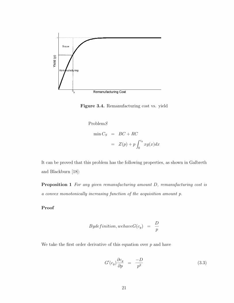
Figure 3.4. Remanufacturing cost vs. yield
ProblemS
minCS = BC +RC
= Z(p) + p∫ cy
0xg(x)dx
It can be proved that this problem has the following properties, as shown in Galbreth
and Blackburn [18]:
Proposition 1 For any given remanufacturing amount D, remanufacturing cost is
a convex monotonically increasing function of the acquisition amount p.
Proof
Bydefinition, wehaveG(cy) =D
p
We take the first order derivative of this equation over p and have
G′(cy)∂cy∂p
=−Dp2
(3.3)
21

After reorganization, we have
∂cy∂p
=−D
p2G′(cy)(3.4)
If we take partial derivative of Eqn. (3.4) over p and substitute (3.3) into the result,
we have
∂2cy∂p2
=2D
p3G′(cy)+G′′(cy)
D2
p4[G′(cy)]3(3.5)
Therefore, if we take the first order derivative of RC over p, we have
∂RC(p)
∂p=
∂p∫ cy
0 xg(x)dx
∂p
=∂cyD − p
∫ cy
0 G(x)dx
∂p
= D∂cy∂p−∫ cy
0G(x)dx− pG(cy)
∂cy∂p
= −∫ cy
0G(x)dx
≥ 0 (3.6)
If we take derivative of (3.6) over p, we have
∂2RC(p)
∂p2=
D2
p3G′(cy)≥ 0 (3.7)
Combine Eqn. (3.6) and 3.7, we know RC(p) is monotonously increasing convex
function.
Proposition 2 Given any convex acquisition cost, the total cost CS(p) is convex.
Therefore, there is an optimal acquisition amount p∗ and corresponding optimal re-
manufacturing cost threshold c∗y which minimizes total average costs to meet a fixed
demand.
22

Proof From Proposition 1, we know RC(p) is convex. Therefore, as long as the
acquisition cost BC(p) is convex, their summation, CS(p) is also convex.
3.4. Model Analysis
3.4.1 Linear Acquisition Cost
As we have proved the convexity of the objective function and hence the existence
of the minimal total cost, we show how to obtain this optimum when the acquisition
cost is linear. That is, we assume
Z(p) = bp
where b is the per unit acquisition cost.
If we take the first order condition of the objective function over p and substitute
the Eqn. (3.6) into the result, we will have
b =∫ cy
0G(x)dx (3.8)
From Eqn. (3.8), we have the following proposition:
Proposition 3 In a single period, if the acquisition cost is linear, the minimal cost
can be achieved at an optimal yield, which is independent of the actual acquired
amount.
Proof We define
F (x) =∫ x
0G(t)dt
As G(t) is an positive increasing function, the inverse of F (x) exists. Therefore, we
can solve Eqn. (3.8) and find the optimal cost threshold
c∗y = F−1(b)
23

and the corresponding optimal yield
y∗ = G(c∗y)
Since the optimal yield is independent of the total acquisition quantity, the determin-
istic demand restriction can actually be relaxed. Therefore, as long as the acquisition
cost is linear in the quantity, the optimal acquisition and sorting problem may be
solved as general inventory problems which may include setup costs, backlogging and
uncertain demand.
3.4.2 Piecewise Linear Cost
While Galbreth and Blackburn [18] have shown the convexity of the objective
function when the acquisition cost is convex increasing, they stop there and continue
to work on linear acquisition cost for their remaining study. In this section, we
extend this work and analyze the case when acquisition cost is a piecewise linear
convex function. Assume the acquisition cost has the form
Z(p) =
b1p+ η1, if p ∈ [0, q1)
b2p+ η2, if p ∈ [q1, q2)
· · ·
bmp+ ηm, if p ∈ [qm−1, qm)
(3.9)
We prove this case has the following properties.
Proposition 4 The optimal cost threshold c∗y of the piecewise linear acquisition cost
problem is
c∗y =
c∗yi , if qi−1G(c∗yi) ≤ D < qiG(c∗yi)
G−1(Dqi
), if qiG(c∗yi) ≤ D < qiG(c∗yi+1)
24
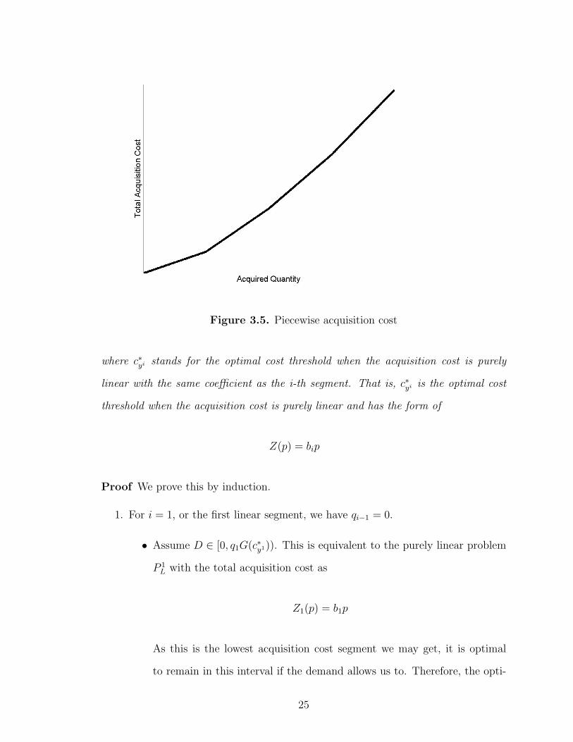
Figure 3.5. Piecewise acquisition cost
where c∗yi stands for the optimal cost threshold when the acquisition cost is purely
linear with the same coefficient as the i-th segment. That is, c∗yi is the optimal cost
threshold when the acquisition cost is purely linear and has the form of
Z(p) = bip
Proof We prove this by induction.
1. For i = 1, or the first linear segment, we have qi−1 = 0.
• Assume D ∈ [0, q1G(c∗y1)). This is equivalent to the purely linear problem
P 1L with the total acquisition cost as
Z1(p) = b1p
As this is the lowest acquisition cost segment we may get, it is optimal
to remain in this interval if the demand allows us to. Therefore, the opti-
25

mal yield we should follow is the optimal yield for problem P 1L, which we
denoted as G(c∗y1). We can see this by contradiction: if we have another
optimal yield G(c∗y) 6= G(c∗y1), which gives a lower total cost, then G(c∗y)
should also be the optimal yield for problem P 1L, instead of G(c∗y1). This
contradicts with our conclusion in the last section.
• Assume D ∈[q1G(c∗y1), q1G(c∗y2)
). The optimal acquisition amount will be
fixed at p = q1 and the optimal yield will increase linearly as the demand
D increases. This can also be proved by contradiction: if it does not hold,
the “optimal acquisition quantity” will lie in [0, q1) or in (q1, q2]. We may
define two corresponding linear problem P 1L and P 2
L, so that their respective
acquisition costs are
Z1 = b1p
Z2 = b2p
Suppose the quantity is in [0, q1). Follow the similar argument as the proof
above, we know problem P 1L will have a new optimal yield G(c∗y) 6= G(c∗y1),
which contradicts with the fact that c∗y1 is its optimal.
Similarly, we can argue the acquisition quantity can not be in (q1, q2].
Therefore, it is bounded at p = q1. While the demand increases, only
the yield (Dp
) increases proportionally, until the cut-off cost reaches c∗y2 .
When the demand further increase after this, the acquisition quantity will
increase and enter the second linear segment.
2. Assume our proposition holds for all i < k.
3. Now we prove our proposition holds for i = k.
26

• Assume D ∈ [qk−1G(c∗yk), qkG(c∗yk)). When the demand increases from
below into this region, the decision maker may choose to keep the previous
yield or apply a new (and higher) yield. We prove it is optimal to apply
the yield G(c∗yk) in this interval by contradiction. Assume some other yield
G(c∗y) 6= G(c∗yk) leads to a lower total cost. Following similar arguments
in i = 1 case, we know this contradicts with the fact that G(c∗yk) is the
optimal yield for the corresponding purely linear problem P kL . Hence, we
know G(c∗y) = G(c∗yk)
• Assume D ∈ [qkG(c∗yk), qkG(c∗yk+1), ).As in i = 1, when the demand further
increase to this region, the optimal acquisition quantity will be fixed at
p = qk so that the optimal yield increases linearly as the demand increases.
Otherwise, it will contradict with the optimal yield we arrived for the
purely linear problems.
Therefore, combining the proof above, our proposition holds for all i’s.
In the next section, we use a numerical example to illustrate this proposition.
3.5. Numerical Study
We proceed our study on the piecewise linear cost problem with a numerical
example to generate further insight.
In this example, we assume the acquisition cost takes the functional form:
Z(p) =
p, p ≤ 2500
2p− 2500, p > 2500
as shown in Figure (3.6) and the remanufacturing yield curve follow a Γ(5, 2) distri-
bution with a mean cost of 10. The cumulative distribution and probability density
functions of Γ(5, 2) are plotted in Figure (3.7). We sweep the demand D from 1 unit
27

Figure 3.6. Acquisition cost vs. acquired quantity, piece-wise linear
to 4999 units and search the acquisition units from D+1 to D+6000 for the minimal
total cost. Figure (3.8) illustrates the relationship between the optimal yield D/p
and the demand D. From the last section, we know the optimal yield should have
the form as
c∗y =
c∗y1 = F−1(1) = 0.4156, if 0 ≤ D
p< 2500× 0.4156 = 1039
G−1( D2500
), if 1039 ≤ D < 2500× 0.5959 = 1490
c∗y2 = F−1(2) = 0.5959, if D ≥ 1490
which agrees well with the numerical results in the figure.
Figure (3.9) shows the relationship between the total cost and the demand. Since
the optimal yield is independent on the actual acquisition quantity, we know the
total cost increases linearly when the acquisition cost is purely linear. It will also
hold in the piecewise linear problem when the yield is still independent on the total
amount. That is, when D ∈ [qi−1G(c∗yi , qiG(c∗yi)). However, this does not hold when
D ∈ [qiG(c∗yi), qiG(c∗yi+1)). In our numerical example, that is to say, the total cost
28

Figure 3.7. Distribution of Γ(5, 2)
Figure 3.8. Optimal yield vs. demand
29

Figure 3.9. Total cost vs. demand
is not proportional to the total amount, when D ∈ [1039, 1490). When we further
increase the demand so that D ∈ [qiG(c∗yi+1), qi), the total cost will increase linearly
again. We can actually show the relationship when D ∈ [qiG(c∗yi), qiG(c∗yi+1)) by
taking first order derivative of the total cost over the demand. As we know, in that
region,
G(cy) =D
qi
Since the total acquisition is fixed at p = qi, when we take the first order derivative
over D, we have
∂cy∂D
=1
qig(cy)(3.10)
Therefore, since
Zi(p) = bip+∫ cy
0xg(x)dx (3.11)
we may take the first order derivative of Eqn. (3.11) and substitute with Eqn. (3.10).
Then we have
30

Figure 3.10. Total cost, optimal yield vs. optimal acquisition
∂Zi
∂D= cyg(cy)
∂cy∂D
=cyqi
Hence, the marginal total cost increases as the demand increases. Figure (3.10)
illustrates that p is fixed in the transition region, which also agrees with our arguments
in the last section.
31

CHAPTER 4
MULTI-PERIOD OPTIMAL ACQUISITION ANDSORTING POLICIES
In this chapter, we extend the single period model to multiple periods. In section
1, we list the assumptions used. Then we explain the notation, and model components
in section 2. We give the full optimization problem formulation in section 3.
After the general descriptions of the model, we prove the convexity of the total
cost. At the end of this chapter, we focus on a special case: linear acquisition cost.
While we have assumed only remanufactured products are kept in inventory, at the
end of this chapter, we relax this constraint and show an example when the unsorted
cores are kept in inventory as well. The motivation for this relaxation comes from
the idea that, in some situations, it is worthwhile or cheaper to keep the unprocessed
cores instead of the final products.
4.1. Model Assumptions
Here, we model how acquisition costs and remanufacturing costs vary over a plan-
ning horizon and find the optimal acquisition and sorting decision, in the sense of
lowest total cost to satisfy demand over the planning horizon.
In our analysis, we assume the demand for remanufactured products at each period
is deterministic. It is denoted as Di in period i and always to be satisfied from
the stock of refurbished products. That is, backlogging is not allowed here. This
assumption separates the channel for remanufacturing products from the channel for
new products. However, in the subsequent sections, we will see the deterministic
demand restriction can actually be relaxed, thanks to the properties of this problem.
32

Figure 4.1. Model Time Line
Again, to simplify our model, we assume the returned cores are either remanufac-
tured or scrapped. No other alternative such as raw material recycling is considered.
Those alternatives can always be handled in our model if scrapping cost is introduced.
The flowchart of the remanufacturing processes is similar to what we have shown
in Figure (3.1). At the beginning of period i, where i = 1, 2, · · ·, T , the firm needs
to determine the total acquisition of pi products from the market or dealers. The
sorting process follows immediately after the acquisition and decides among them ri
items to be remanufactured and the rest pi − ri to be scrapped (pi ≥ ri). At this
moment, we will first assume no unprocessed core will be kept in the inventory. This
makes economic sense, since, otherwise, the remanufacturer should wait instead of
buy back, as the acquisition cost decreases as quality decays in time. However, there
are cases when the remanufacturers decide to acquire earlier so that they may obtain
cores with high quality. They may decide to store unprocessed cores, for the sake of
easy storage, easy transportation, and etc. At the end of this chapter, we will study
the cases where unprocessed cores are allowed to be kept in inventory.
We assume demands are met from the output or the inventory at hand. Remaining
items will be kept in inventory to meet future demands, at some holding cost. The
time line is shown in Figure 4.1.
We keep the perfect testing assumption as before. That is, at the time of sorting,
the corresponding remanufacturing cost is known based on the observed condition.
33

Over the T periods, the decision maker faces the following problem. As the
product condition is variable, some of the units acquired may be too costly to recover
and are, hence, scrapped. As the acquisition amount is increased, sorting can be
made more stringent– only products with lower remanufacturing costs are actually
remanufactured. Of course, the cost of acquiring more used products offsets, to some
extent, the remanufacturing cost savings achieved by increased selectivity. Moreover,
over the planning horizon, the acquisition cost is assumed to be a decreasing function
of time, which simply means the longer the customers use the products, the less they
can sell back to the remanufacturer for.
To capture the time decaying effect of product condition, the remanufacturing cost
is an increasing function of time, which implies that the longer the products have been
used, the more efforts the remanufacturer may have to make to recover them. The
interaction of these effects will drive the acquisition amount and corresponding sorting
policy.
With these assumptions at hand, we are now ready to describe the model in the
next section. Firstly, we introduce the notation to be used and then the three cost
components, namely, the acquisition cost, the remanufacturing cost and the inventory
holding cost. After introducing the cost structure, we derive the constraints that link
multiple periods.
4.2. Model Description
4.2.1 Notation
i: 1, 2, · · ·, T , subscript of periods
Di: the demand for period i;
T : the length of the total planning horizon;
34

h: the per-unit-item and per-unit-time inventory holding cost for the remanufactured
product;
pi: the number of items bought back at the beginning of period i;
cyi: the remanufacturing cost threshold in period i; we use the subscript y, as this
threshold is directly related to the yield;
Zi(pi): the total acquisition cost at the beginning of period i, given pi items to buy
back. This should be a decreasing function of i (time);
Gi(x): the cumulative distribution function, or yield function, of a used product’s
remanufacturing cost at the beginning of period i. In other words, Gi(x) rep-
resents the fraction of the returns that can be remanufactured at cost less than
or equal to x. This is a decreasing function of i (time);
gi(x): the corresponding density function of Gi(x);
ri: the number of items remanufactured at the beginning of period i;
Ii: inventory at the end of period i;
BCi: the acquisition cost for period i;
BC: the total acquisition cost over the horizon;
RCi: the remanufacturing cost for period i;
RC: the total remanufacturing cost over the horizon;
ICi: the inventory cost for period i;
IC: the total inventory cost over horizon;
35

Figure 4.2. Acquisition cost for different periods.
4.2.2 acquisition Cost
As reasoned in the first section, given any fixed number of acquired units, the
acquisition costs are assumed to decrease in time, which simply means the longer
the customers use the product, the less they can sell back to the remanufacturer
for. Figure 4.2 illustrates the total acquisition cost function family for the first three
periods.
We assume the marginal acquisition cost is a non-decreasing function in acquired
quantity, because of scarcity. Therefore, we denote the total acquisition cost for each
period as
BCi = Zi(pi) (4.1)
While we do not assume specific function form here, Zi’s are linear or convex increas-
ing function of their arguments pi, or Z ′′i (pi) ≥ 0 to account for the non-decreasing
property of non-decreasing marginal cost.
36

Figure 4.3. Remanufacturing cost for different periods.
The total acquisition cost is
BC =T∑
i=1
BCi
=T∑
i=1
Zi(pi) (4.2)
Note here, we do not introduce extra discount factor, since it can always be introduced
into the decaying acquisition cost.
4.2.3 Remanufacturing Cost
Figure 4.3 illustrates the total remanufacturing cost for the first three periods.
Again, we are incorporating the idea of non-decreasing marginal remanufacturing
cost into our model. However, unlike the acquisition cost, the remanufacturing cost
increases in time, which implies that the longer the products have been used, the
more efforts the remanufacturer may have to make to recover them.
37

Figure 4.4. Remanufacturing cost - Yield for different periods.
For given acquisition quantity at any period, the remanufacturing quantity is
equivalent to remanufacturing yield (denoted as y) and we re-plot its relationship to
remanufacturing cost in Figure 4.4. Because the remanufacturing cost can represent
the condition of the returned core, these yield functions can be viewed as cumulative
distribution functions for the quality and we denote them as Gi(cyi), and the corre-
sponding probability density function gi(cyi). When the remanufacturer decides to
remanufacture products at cost no higher than cyi(we term it remanufacturing cost
threshold), the yield it can realize is given by y = Gi(cyi).
Hence, for each period, the remanufacturing cost is
RCi = ri
∫ cyi0 xgi(x)dx∫ cyi0 gi(x)dx
= pi
∫ cyi
0xgi(x)dx (4.3)
and the total remanufacturing cost is
38

RC =T∑
i=1
RCi
=T∑
i=1
pi
∫ cyi
0xgi(x)dx (4.4)
4.2.4 Inventory Cost
While all the remanufacturing or scrapping decisions are made immediately after
the acquisition, it is possible to hold inventory for the refurbished products to the
successive periods at some cost.
The inventory cost for each period is given as
ICi = hIi +1
2hDi (4.5)
where the second term is average holding cost for the products sold in this period.
The total inventory cost is
IC =T∑
i=1
ICi
=T∑
i=1
(hIi +1
2hDi) (4.6)
4.2.5 Inventory Constraints
The inventory cost should satisfy the following constraints
I0 = 0
Ii = Ii−1 −Di + ri, where i = 1, 2, ..., T − 1
Ii ≥ 0
IT = 0
39
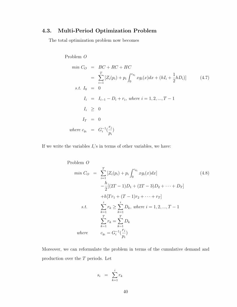
4.3. Multi-Period Optimization Problem
The total optimization problem now becomes
Problem O
min CO = BC +RC +HC
=T∑
i=1
[Zi(pi) + pi
∫ cyi
0xgi(x)dx+ (hIi +
1
2hDi)] (4.7)
s.t. I0 = 0
Ii = Ii−1 −Di + ri, where i = 1, 2, ..., T − 1
Ii ≥ 0
IT = 0
where cyi= G−1
i (ri
pi
)
If we write the variables Ii’s in terms of other variables, we have:
Problem O
min CO =T∑
i=1
[Zi(pi) + pi
∫ cyi
0xgi(x)dx] (4.8)
−h2
[(2T − 1)D1 + (2T − 3)D2 + · · ·+DT ]
+h[Tr1 + (T − 1)r2 + · · ·+ rT ]
s.t.i∑
k=1
rk ≥i∑
k=1
Dk, where i = 1, 2, ..., T − 1
T∑k=1
rk =T∑
k=1
Dk
where cyi= G−1
i (ri
pi
)
Moreover, we can reformulate the problem in terms of the cumulative demand and
production over the T periods. Let
si =i∑
k=1
rk
40

cyi= G−1
i (ri
pi
) = G−1i (
si − si−1
pi
)
Ei =i∑
k=1
Dk
const1 =1
2hET
then we can write the problem as
Problem S
min CS =T∑
i=1
[Zi(pi) + pi
∫ cyi
0xgi(x)dx] + h
T∑i=1
(si − Ei) + const1
s.t. si ≥ Ei, where i = 1, 2, ..., T − 1
sT = ET
Note that we may also remove the equality constraint in Problem O and Problem
S by embedding it into the objective function. Therefore, another simplified version
is
Problem O’
min CO′ =T∑
i=1
[Zi(pi) + pi
∫ cyi
0xgi(x)dx]
−h2
[(2T − 3)D1 + (2T − 5)D2 + · · ·+DT−1 −DT ]
+h[(T − 1)r1 + (T − 2)r2 + · · ·+ rT−1]
s.t.i∑
k=1
rk ≥i∑
k=1
Dk, where i = 1, 2, ..., T − 1
where cyi= G−1
i (ri
pi
)
and
Problem S’
41

min CS′ =T∑
i=1
[Zi(pi) + pi
∫ cyi
0xgi(x)dx] + h
T−1∑i=1
(si − Ei) + const1
s.t. si ≥ Ei, where i = 1, 2, ..., T − 1
As the problems above are equivalent, we may apply different forms when that one
is easier for derivation.
In the next section, we prove the convexity of the objective function.
4.4. Convexity of the Cost Function
We first prove the following two propositions.
Proposition 5 The function CO(r1, r2, · · · , rT , p1, p2, · · · , pT ) is convex, if the acqui-
sition cost functions Zi’s are strictly convex.
Proof Before we continue, we need put down some important relationships here:
∂cyi
∂ri
=1
pigi(cyi)
∂2cyi
∂r2i
=−g′i(cyi
)
p2i g
3i (cyi
)
∂cyi
∂pi
=−ri
p2i gi(cyi
)
∂2cyi
∂p2i
=2pirig
2i (cyi
)− r2i g′i(cyi
)
p4i g
3i (cyi
)
∂2cyi
∂ri∂pi
=rig′i(cyi
)− pig2i (cyi
)
p3i g
3i (cyi
)
and hence
∂CO
∂ri
= cyi+ h(T + 1− i)
∂2CO
∂r2i
=1
pigi(cyi)
∂2CO
∂ri∂pi
=−ri
p2i gi(cyi
)
42

∂CO
∂pi
= Z ′i(pi)−∫ cyi
0Gi(x)dx
∂2CO
∂p2i
= Z ′′i (pi) +Gi(cyi)
ri
p2i gi(cyi
)
= Z ′′i (pi) +r2i
p3i gi(cyi
)
∂2CO
∂pi∂pj
=∂2CO
∂pi∂rj
=∂2CO
∂ri∂rj
= 0 (i 6= j)
The Hessian matrix for CO has the following form
H(CO) =
∂2CO
∂r21, ∂2CO
∂r1∂r2, · · · , ∂2CO
∂r1∂rT, ∂2CO
∂r1∂p1, ∂2CO
∂r1∂p2, · · · , ∂2CO
∂r1∂pT
∂2CO
∂r2∂r1, ∂2CO
∂r22, · · · , ∂2CO
∂r2∂rT, ∂2CO
∂r2∂p1, ∂2CO
∂r2∂p2, · · · , ∂2CO
∂r2∂pT
......
......
......
......
∂2CO
∂rT ∂r1, ∂2CO
∂rT ∂r2, · · · , ∂2CO
∂r2T, ∂2CO
∂rT ∂p1, ∂2CO
∂rT ∂p2, · · · , ∂2CO
∂rT ∂pT
∂2CO
∂p1∂r1, ∂2CO
∂p1∂r2, · · · , ∂2CO
∂p1∂rT, ∂2CO
∂p21, ∂2CO
∂p1∂p2, · · · , ∂2CO
∂p1∂pT
∂2CO
∂p2∂r1, ∂2CO
∂p2∂r2, · · · , ∂2CO
∂p2∂rT, ∂2CO
∂p2∂p1, ∂2CO
∂p22, · · · , ∂2CO
∂p2∂pT
......
......
......
......
∂2CO
∂pT ∂r1, ∂2CO
∂pT ∂r2, · · · , ∂2CO
∂pT ∂rT, ∂2CO
∂pT ∂p1, ∂2CO
∂pT ∂p2, · · · , ∂2CO
∂p2T
.
This proof is divided into two parts, namely, when T = 2 and when T > 2. As we
only consider multi-period problem, we assume T ≥ 2. T = 1 has been shown in by
Galbreth and Blackburn [18].
1. T = 2
The Hessian matrix becomes
H(CO) =
1p1g1(cy1 )
, 0, −r1
p21g1(cy1 )
, 0
0, 1p2g2(cy2 )
, 0, −r2
p22g2(cy2 )
−r1
p21g1(cy1 )
, 0, Z ′′1 (p1) +r21
p31g1(cy1 )
, 0
0, −r2
p22g2(cy2 )
, 0, Z ′′2 (p2) +r22
p32g2(cy2 )
.
43

We study the leading principal minors, represented as Hk for the k degree
leading principal minors, as following:
• H4
H4 =
∣∣∣∣∣∣∣∣∣∣∣∣∣∣∣∣
1p1g1(cy1 )
, 0, −r1
p21g1(cy1 )
, 0
0, 1p2g2(cy2 )
, 0, −r2
p22g2(cy2 )
−r1
p21g1(cy1 )
, 0, Z ′′1 (p1) +r21
p31g1(cy1 )
, 0
0, −r2
p22g2(cy2 )
, 0, Z ′′2 (p2) +r22
p32g2(cy2 )
∣∣∣∣∣∣∣∣∣∣∣∣∣∣∣∣=
1
p1g1(cy1)
1
p2g2(cy2)[Z ′′1 (p1) +
r21
p31g1(cy1)
][Z ′′2 (p2) +r22
p32g2(cy2)
]
+r21
p41g
21(cy1)
r22
p42g
22(cy2)
− r21
p41g
21(cy1)
1
p2g2(cy2)[Z ′′2 (p2) +
r22
p32g2(cy2)
]
− r22
p42g
22(cy2)
1
p1g1(cy1)[Z ′′1 (p1) +
r21
p31g1(cy1)
]
=Z ′′1 (p1)Z
′′2 (p2)
p1g1(cy1)p2g2(cy2)> 0
• H3
H3 =
∣∣∣∣∣∣∣∣∣∣∣∣
1p1g1(cy1 )
, 0, −r1
p21g1(cy1 )
0, 1p2g2(cy2 )
, 0
−r1
p21g1(cy1 )
, 0, Z ′′1 (p1) +r21
p31g1(cy1 )
∣∣∣∣∣∣∣∣∣∣∣∣=
1
p1g1(cy1)
1
p2g2(cy2)[Z ′′1 (p1) +
r21
p31g1(cy1)
]− r21
p41g
21(cy1)
1
p2g2(cy2)
=Z ′′1 (p1)
p1g1(cy1)p2g2(cy2)> 0
• H2
H2 =
∣∣∣∣∣∣∣∣1
p1g1(cy1 ), 0
0, 1p2g2(cy2 )
∣∣∣∣∣∣∣∣44

=1
p1g1(cy1)
1
p2g2(cy2)> 0 (4.9)
• H1
H1 =1
p1g1(cy1)> 0 (4.10)
Therefore, because all the leading principal minors are non-negative, from the
Sylvester criterion, we know H(CO) is positive definite when T = 2.
2. T > 2
The Hessian matrix becomes
H(CO) =
1p1g1(cy1 )
, 0, · · · , 0, −r1p21g1(cy1 )
, 0, · · · , 0
0, 1p2g2(cy2 )
, , · · · , 0, 0, −r2p22g2(cy2 )
, · · · , 0
......
......
......
......
0, 0, · · · , 1pT gT (cyT
), 0, 0, · · · , −rT
p2T
gT (cyT),
−r1p21g1(cy1 )
, 0, · · · , 0, Z′′1 +r21
p31g1(cy1 )
, 0, · · · , 0
0, −r2p22g2(cy2 )
, , · · · , 0, 0, Z′′2 +r21
p31g1(cy1 )
, · · · , 0
......
......
......
......
0, 0, · · · , −rT
p2T
gT (cyT), 0, 0, · · · , Z′′T +
r2T
p3T
gT (cyT)
Note here Z ′′i still represents Z ′′i (pi) and the arguments are omitted to save space.Similar to the T = 2 case, we study the leading principal minors. Observing
the matrix above, it is easy to see all the leading principal minors with degree lessthan 2T are positive, because their only non-zero component is the product of theirdiagonal elements, which are all positive. Therefore, we only need to study the leadingprincipal minor H2T .
H2T =T∏
i=1
1
pigi(cyi)[Z ′′i (pi) +
r2i
p3i gi(cyi
)] + (−1)T 2
T∏i=1
r2i
p4i g
2i (cyi
)
>T∏
i=1
1
pigi(cyi)
r2i
p3i gi(cyi
)−
T∏i=1
r2i
p4i g
2i (cyi
)= 0
Therefore, from the Sylvester criterion, we know H(CO) is positive definite whenT > 2.
45

In conclusion, we proved that the Hessian matrix for CO(r1, r2, · · · , rT , p1, p2, · · · , pT )is positive definite, and therefore, CO is a convex function. While we proved this forT ≥ 2, this can be easily extended to the trivial case when T = 1, though this is notof interest here.
Proposition 6 CS(s1, s2, · · · , sT , p1, p2, · · · , pT ) is convex, if the acquisition cost func-
tions Zi’s are strictly convex.
Proof As we know,
r1 = s1
ri = si − si−1 (i = 2, 3, · · · , T )
or we may write it in matrix form (here, prime represents matrix transpose)
[r1, · · · , rT , p1, · · · , pT ]′ = A× [s1, · · · , sT , p1, · · · , pT ]′
where matrix A is defined as
A =
1
−1 1
−1 1
. . . . . .
−1 1
0 1
. . . . . .
0 1
Therefore, we have
CS(x) = CO(Ax)
46

Because composition with an affine mapping preserves the convexity, CS is convex,
given Proposition 1.
As we have proved the convexity of the function, we may use Karush-Kuhn-Tucker
(KKT) condition to find the global minimum, if it is feasible.
We define Problem L:
Problem L
min CL =T∑
i=1
[Zi(pi) + pi
∫ cyi
0xgi(x)dx]
−h2
[(2T − 3)D1 + (2T − 5)D2 + · · ·+DT−1 −DT ]
+h[(T − 1)r1 + (T − 2)r2 + · · ·+ rT−1]
+T−1∑i=1
ui(i∑
k=1
Dk −i∑
k=1
rk)
where ui ≥ 0
ui(i∑
k=1
Dk −i∑
k=1
rk) = 0, (i = 1, 2, ..., T − 1)
and take its first order derivative conditions
∂CL
∂pi= Z ′i(pi)−
∫ cyi0 Gi(x)dx = 0
∂CL
∂ri= cyi
− cyT+ h(T − i)−
T−1∑k=i
uk = 0
ui(i∑
k=1Dk −
i∑k=1
rk) = 0
i = 1, 2, · · · , T − 1
(4.11)
From the propositions listed above, we have the following theorem:
Theorem 1 If the solution to Eqn. (4.11) is feasible to Problem O, it is also the
optimal solution to Problem O.
Proof Let P =
{(r1, r2, · · · , rT−1, p1, p2, · · · , pT )|
i∑k=1
ri, i = 1, 2, · · · , T − 1 ≥i∑
k=1
Di
}.
That is, P is the feasible set for Problem O. It is easy to see that P is a convex set.
47

If we have solution X = (r∗1, r∗2, · · · , r∗T−1, p
∗1, p∗2, · · · , p∗T ) to Eqn. (4.11); i.e. the
solution to Problem L, and X ∈ P , combining the proposition above that objective
function CO is a convex function, we know that we reach the global minimum of
Problem O, because of the Karush-Kuhn-Tucker (KKT) condition.
4.5. Linear Acquisition Cost Without Core Holding
Prior research ([40, 42, 45]) justifies the linear acquisition as a valid assumption,
particularly when the market is large and well-defined. In this section, we examine
this special case and assume
Zi(pi) = bipi
where bi’s are the per unit acquisition cost for period i and
bi ≥ bj, ( for 1 ≤ i ≤ j ≤ T ).
Hence, the optimization problem reduces to
Problem LR
min CLR =T∑
i=1
[bipi + pi
∫ cyi
0xgi(x)dx] + h
T−1∑i=1
(si − Ei) + const
s.t. si ≥ Ei, where i = 1, 2, ..., T − 1
where cyi= G−1
i (ri
pi
) = G−1i (
si − si−1
pi
)
Given this reduced optimization problem, we have the following proposition:
Proposition 7 For linear acquisition cost, the optimal remanufacturing yield in each
period depends on the per-unit acquisition cost and the remanufacturing cost function,
but it does not depend on the actual demand or acquisition quantity.
48

Proof Define f(p1, p2, · · · , pT ) = CLR(p1, p2, · · · , pT ; s1 = S1, s2 = S2, · · · , sT = ST ),
i.e., we define f as a function of arguments p1, p2, ... and pT , and with the parameter
set s1 = S1, s2 = S2, ... and sT = ST . The partial derivatives are as following:
∂f∂pi
= bi −∫ cyi0 Gi(x)dx
∂2f∂p2
i= (si−si−1)2
p3i gi(cyi )
∂2f∂pi∂pj
= 0 (i 6= j)
(4.12)
Therefore, the Hessian matrix becomes
H(f) =
s21
p31g1(cy1 )
. . .
(sT−sT−1)2
p3T gT (cyT
)
and it is straightforward this Hessian matrix is positive definite. Thus, function f is
convex.
We define Fi(x) =∫ x0 Gi(t)dt. Since Gi(t) > 0 for t ∈ (0, 1], we know the inverse
of Fi(x) exists.
Therefore, from the first order condition in Eqn. (4.12), f takes its minimum at
c∗yi= F−1
i (bi)
which does not depend on the actual demand and acquisition quantity.
Then the optimal yields are given by
c∗yi= F−1
i (bi) (4.13)
where Fi(x) =∫ x
0Gi(t)dt
We define C∗LR(s1, s2, · · · , sT ) as the optimal solution when cyi= c∗yi
. That is, the
minimum cost depends on the parameter set (s1, s2, · · · , sT ).
49

Take the first order derivatives of these parameters, we have
∂C∗LR
∂si
= c∗yi− c∗yi+1
+ h
4.5.1 Special Cases
Now, we first study the solution properties for three special cases.
1. c∗yi− c∗yi+1
+ h > 0 for all i = 1, 2, · · · , T − 1
The minimal cost increases in si. Given the constraints that si ≥ Ei (i =
1, 2, · · · , T − 1), we have
si = Ei
This implies that the remanufacturer should not keep inventory at the end of
period i, given c∗yi− c∗yi+1
+ h > 0. Therefore, the original multiple period
problem is simplified into two sub-problems at any point i.
2. c∗yi− c∗yi+1
+ h = 0 for all i = 1, 2, · · · , T − 1
When this happens, the remanufacturer should be indifferent to the inventory
decision, as long as demand in any period is satisfied.
3. c∗yi− c∗yi+1
+ h < 0 for all i = 1, 2, · · · , T − 1
This implies the minimal cost decreases as si increases. Since we have the
s1 ≤ s2 ≤ · · · ≤ sT , we should have s1 = s2 = · · · = sT = ET . That is, it
is optimal to acquire and remanufacture at the beginning of period 1 and hold
inventory for the following periods.
4.5.2 General Cases
We assume a general linear acquisition cost case as shown in Figure 4.5.
50

Figure 4.5. General Problem with Linear Acquisition Cost
In this figure, positive sign (“+”) represents that c∗yi− c∗yi+1
+h > 0 at this period
and negative sign (“-”) means that c∗yi− c∗yi+1
+ h < 0. The entire time horizon is
assumed to start with a series of “+” periods (t0,1, t0,2, · · · , t0,k0) and we denote them
as set Θ0; that is,
Θ0 =
{t0,i : (c∗yi
− c∗yi+1+ h) > 0
}
Similarly, we assume the horizon ends with a series of “-” periods (tb,1, tb,2, · · · , tb,kb)
and denote them as set Θb, or
Θb =
{tb,i : (c∗yi
− c∗yi+1+ h) < 0
}
However, these assumptions do not sacrifice the generosity here, since we allow Θ0
and Θb to be null sets. We will include the c∗yi− c∗yi+1
+ h = 0 at the end of this
section.
si’s within Θ0 and Θb can be determined easily:
1. Θ0
Since the total cost increases in the si’s within this set, the optimum will be
achieved when they are at their minimum. Given the no backlogging constraints,
we have
s0,i = E0,i, where i = 1, · · · , k0
51

Figure 4.6. General Solution with Linear Acquisition Cost
Figure 4.7. Base of General Solution for one Set
2. Θb
As the cost decreases in si’s within this set, to obtain optimum, si’s should be
all equal to ET here. That is,
sb,i = ET , where i = 1, · · · , kb
We separate the rest portion of the time horizon (except Θ0 and Θb) into (b− 1)
sets, such that each set i starts with a series of “-” periods (ti−,j−i’s) and ends with
“+” ones (ti+,j+i
’s). Here, j−i ∈{
1, 2, · · · , k−i}
and j+i ∈
{1, 2, · · · , k+
i
}, where k−i and
k+i is the total number of “-” and “+” periods in set i, respectively.
4.5.2.1 Solution for a Single Set
Figure 4.6 illustrates one such set i. The symbols above the time line represent the
beginning point of the periods, and the symbols below are the corresponding values
of si’s. Note while s(ti+/−,j) actually stands for sti+/−,j
, we use the former to make
the figure discernible. This is also the reason why we use E(ti+/−,j) instead of Eti+/−,j
in Figure 4.8.
The general solution for the set in Figure 4.6 can be obtained as
52

1. “-” periods:
As discussed above, when c∗yi− c∗yi+1
+ h < 0, the total cost decreases in si and
it is optimal to maximize those si’s while still satisfying the constraints: si ≤ sj
(for i < j) and si ≥ Ei. Therefore, we have
s(ti−,1) = s(ti−,2) = · · · = s(ti−,k−i) = s(ti+,1)
2. “+” periods:
Following the similar reasoning, when c∗yi− c∗yi+1
+ h > 0, si should be as small
as possible and satisfies the constraints above. Hence, we have
s(ti+,c) = max{s(ti+,1), E(ti+,j)
}where j = 1, 2, · · · , k+
i
We define a base solution for this problem, shown in Figure 4.7. From the reason-
ing above, we know the optimal solution has the property that, at any period, st+/−,j
should be no less than the value shown in this base solution. Therefore, to solve the
problem, we may start from the base and then sum up the equation c∗yi− c∗yi+1
+ h
for all “-” periods. That is, let
S =k−i∑j=1
c∗y(ti−,j)− c∗y(ti−,j+1) + h = c∗y(ti−,1) − c∗y(ti+,1) + k−i h
From this point on, we adapt the following steps:
• Step 1: let j = 1.
• Step 2: let S = S + c∗y(ti+,j)− c∗y(ti+,j+1) + h
• Step 3: if S ≤ 0, for t = t(i+, 1), t(i
+, 2), · · · , t(i+, j − 1), t(i+, j), raise the value
for all s(t)’s to E(ti+,j), set j = j + 1 and return to step 2; otherwise, continue
to Step 4
53

Figure 4.8. Base of General Solution
• Step 4: for the remaining periods (t = t(i+, j + 1), · · · , t(i+, k+
i )) let s(t) =
E(t).
Proof The proof of this algorithm follows directly from the idea that, as long as the
cumulative sum S is negative, we may further reduce the total cost by raising all the
si’s before the time t = j
4.5.2.2 Solution for General Cases
With the conclusions above, we can solve a general linear acquisition cost problem
following the procedures below:
• Step 1: Obtain all c∗yi’s from Equation (4.13)
• Step 2: Start with the base solution as shown in Figure 4.8.
• Step 3: For periods t0,i’s, fix s0,i = E(t0,i). Similarly, for periods tb,ib ’s, let
sb,ib = ET .
• Step 4: Starting from period t1−,1, keep calculating cumulative sum S as
S = S + c∗y(ti+,j)− c∗y(ti+,j+1) + h
until S becomes positive at some period t = ti+,j′ (Note, this can only happen
at some positive periods). Raise all the sti+,j’s to E(ti+,j′), where j ≤ j′.
54

• Set all the remaining sti+,j’s (where j = j′ + 1, j′ + 2, · · · , k+
i ) to their allowed
minimum. That is, sti+,j= E(ti+,j). In another words, keep them as in the base
solution.
• Step 5: If i+ 1 6= b, starting from period t = t(i+1)−,1, treating it as t1−,1, reset
S = 0 and go back to step 4. Otherwise, end the process and we have reached
the solution.
4.5.2.3 Quantity-Independent Optimal Yield
In this section, we will study the linear acquisition cost problem again in terms of
quantity-independent optimal yield.
The equation (4.13) gives the optimal remanufacturing cost threshold, which does
not depend on the actual amount desired to remanufacture. Therefore, for products
acquired, remanufactured and then sold in period i, the total cost is given by
TCi = bipi + pi
∫ c∗yi
0xgi(x)dx
and hence, the average per unit is
ATCi = bi/y∗i + A∗i
where we define
y∗i = Gi(c∗yi
)
A∗i =
∫ c∗yi0 xgi(x)dx∫ c∗yi0 gi(x)dx
Similarly, if these items are held in inventory and sold in period j (j ≥ i), their
average cost is
ATCi = bi/y∗i + A∗i + (j − i)h
55

The last component is introduced to count for the inventory holding cost. Therefore,
we can prove the following proposition.
Proposition 8 For the linear acquisition cost case above, the optimal average cost
per unit in period i is given by
minj=1,···,i
(bj/y∗j + A∗j + (j − i)h) (4.14)
Proof First of all, it is obvious that the optimal average cost in period i is no
greater than in (4.14). Assume that k = arg{ minj=1,···,i
(bj/y∗j + A∗j + (j − i)h)}. the
remanufacturer may acquire, remanufacture and hold inventory in period k alone to
satisfy the demand in period i. Given the average cost does not change with the
amount actually required, the average cost can always be realized with such policy.
Now we show that the optimal average cost cannot be lower than (4.14). Assume
there exists another policy to satisfy the demand in period i, with lower average
cost than in this proposition, and assume that policy requires the remanufacturer to
acquire, remanufacture and hold kj units in inventory from period j (j = 1, · · · , i)
to satisfy the demand of period i. That is, Di =i∑
j=1kj. Therefore, there must
exist at least one period k∗ (k∗ ∈ 1, · · · , i) where the average cost is lower than
ATCk∗ = bk∗/y∗k∗ + A∗k∗ , which contradicts with the conclusion we have reached that
the optimal cost is given by (4.13).
From this proposition, we may reach the optimal remanufacturing cost for all periods
and thus the original problem reduce to a linear programming problem.
4.6. Linear Acquisition Cost With Core Holding
Till this point, we have made the assumption that the cores, once acquired, are
inspected and remanufactured immediately. In practice, however, this may not hold
for various reasons. For example, the inventory holding cost for raw cores may be
56

lower than for final products; or it may be harder to transport raw cores. Therefore,
in this section, we study the cases where both inventory for uninspected raw cores
and final products can be kept in inventory. However, we still assume inspected cores
are remanufactured or discarded immediately after the inspection.
Unlike when raw cores inventory is not held, in each period, now we have two
different sources for final products. We may acquire cores in previous period, hold
them uninspected and remanufacture when we need them; or we may acquire, re-
manufacture and hold them as final products in inventory. However, it is easy to rule
out other options. That is, it can never be optimal to acquire the raw cores and hold
them for portion of the time, remanufacture then and hold the final products for the
rest portion of time.
The reason is as following:
• If the average holding cost for raw cores is lower than for the final products,
they should be kept in the form of raw cores until when they are needed, to
save the inventory cost, since the remanufacturing yield-cost relationship does
not change over time.
• Similarly, if the holding cost for raw cores is higher than for the final products,
they should be kept in the form of final products ever since they are acquired.
4.6.1 A Simple Case
Before we continue with the study, we first study a simple case where inventory
is only kept for uninspected raw cores, at the per unit cost of hr per time period.
That is, after acquisition, the remanufacturer decides the portion to inspect and then
remanufacture or discard, and the rest is kept as raw cores. Final products are either
used to satisfy demand or discarded. No inventory will be kept for them.
For period i, this is equivalent to say there are i different sources of raw cores,
each of which may reduce to a similar problem as in the last section. That is, for raw
57

cores acquired at period j and held to period i, we may consider them as acquired
at period i with acquisition cost bj + (i − j)hr and the remanufacturing cost-yield
relationship Gj(x). Therefore, following the same derivation as before, we may get
the optimal average cost per unit as
ATCj,i = [bj + (i− j)hr]/y∗j,i + A∗j,i (4.15)
where
y∗j,i = Gj(c∗yj,i
)
c∗yj,i= F−1
j (bj + (i− j)hr) (4.16)
A∗j,i =
∫ c∗yj,i
0 xgj(x)dx∫ c∗yj,i
0 gj(x)dx
The minimum average cost for any period i will be achieved by solving the linear
problem:
ATC∗i = minj=1,···,i
[bj + (i− j)hr]/y∗j,i + A∗j,i (4.17)
The algorithm to solve this problem is
• Step 1: Obtain c∗yj,i’s from Equation (4.16) for i = 1, · · · , T and j = 1, · · · , i;
• Step 2: Solve the minimal average cost problem in (4.17) for period i (i =
1, · · · , T ) and obtain j∗i , so that
j∗i = arg minj=1,···,i
{[bj + (i− j)hr]/y∗j,i + A∗j,i} (4.18)
Also, let rj∗,i = Di and pj∗,i =rj∗,i
Gj(c∗yj,i)
58

• Step 3: For each period j∗, let pj∗ =T∑
i=j∗pj∗,i, which is the total units should
be acquired. Moreover, pj∗,i’s are the cores acquired at period j∗ and kept in
inventory to satisfy the demand in period i.
4.6.2 Linear Acquisition Cost With Core Holding
Now we are ready to study the original problem. That is, both raw cores and re-
manufactured products may be kept in inventory. At any period, the remanufacturer
has two options:
• use the final products remanufactured before;
• inspect and remanufacture the raw cores acquired before.
The first option is equivalent to the problem we solved before, or the linear acquisition
cost case without core holding; while the second option is equivalent to what we
derived above. As both case give the optimal yield independent on the actual amount
desired, the decision maker should always use the one which gives the lower per unit
cost, instead of any combination of the two. If we let hr represent per unit holding
cost for raw cores and hf for final products, we will have the optimal average cost for
period i from the minimum of Eqn. (4.14) and Eqn. (4.17):
ATC∗i = min
{min
j=1,···,i
{[bj + (i− j)hr]/y
∗j,i + A∗j,i
}, minj=1,···,i
{(bj/y
∗j + A∗j + (j − i)hf )
}}(4.19)
where
c∗yi= F−1
i (bi)
c∗yj,i= F−1
j (bj + (i− j)hr)
y∗i = Gi(c∗yi
)
y∗j,i = Gj(c∗yj,i
)
59

A∗i =
∫ c∗yi0 xgi(x)dx∫ c∗yi0 gi(x)dx
A∗j,i =
∫ c∗yj,i
0 xgj(x)dx∫ c∗yj,i
0 gj(x)dx
Therefore, the linear acquisition cost problem with core holding can be solved in
the following steps:
• Step 1: Obtain all c∗yiand c∗yj,i
’s from above.
• Step 2: Solve the minimal average cost problem in (4.19) for period i (i =
1, · · · , T ) and obtain j∗i , so that
j∗i = arg min
{min
j=1,···,i
{[bj + (i− j)hr]/y
∗j,i + A∗j,i
}, minj=1,···,i
{(bj/y
∗j + A∗j + (j − i)hf )
}}
If the left component is the minimum, the demand in period i should be sat-
isfied by the raw cores acquired at period j∗i , and remanufactured at period i.
Otherwise, or if the right component is the minimum, the demand in period i
should be satisfied by the final products acquired, remanufactured and carried
from period j∗i
• Step 3: From step 2, the total amount of acquiring and remanufacturing at each
period is known.
Similar to the single period model, since the optimal yield is independent of the
total acquisition quantity, the deterministic demand restriction can actually be re-
laxed. Therefore, as long as the acquisition cost is linear in the quantity, the optimal
acquisition and sorting problem may be solved as general inventory problems which
may include setup costs, backlogging and uncertain demand.
60

CHAPTER 5
CONCLUSIONS
The fast development of new technologies has brought an amazing array of high-
tech consumer products. However, they have also brought an equally astounding
profusion of electronic waste, among which lead, mercury and other heavy metals
pose serious issues to the environment. In its January issue, National Geographic re-
ported that much of the world’s electronic waste ends up in Ghana and Nigeria, where
children are paid pennies a day to salvage the choice commodities inside–exposing
themselves to dioxins, lead and other poisons. The rest of the waste, spanning every-
thing from dot-matrix printers to surge protectors, ends up scattered in open dumps
or washed out to sea.
On the other hand, much of this electronic waste is in functionally good condition.
In a recent issue of Business Week [10], the author reported a Greenwish CT based
private equity firm, which sensed opportunity in discarded computers and invested
$50 million in TechTurn, an e-recycler. It refurbishes the waste from companies and
sells it to schools, nonprofits and poor countries. In 2007, the company booked $40
million in sales.
As more and more business comes to realize the profitability in this industry,
our study provides a detailed analysis of optimal acquisition and sorting for reman-
ufacturers facing variable condition of the returned cores in both single and multiple
periods. As an extension of Galbreth and Blackburn [18], we first reproduce the re-
sults from those authors. It has been shown that, in single period model, when the
acquisition cost is linear in the acquisition quantity, the optimal yield is independent
61

on the total acquisition amount. In that circumstance, whatever demand it has, the
firm will always follow a simple optimal yield.
We extend this result to the case of piecewise linear convex acquisition costs.
It has been shown that the optimal yield can be obtained by solving linear cost
problems corresponding to its linear segments. When the cost is piecewise linear, the
remanufacturer should still follow the optimal yield as if the cost is purely linear.
However, when the optimal acquisition quantity reaches the intersect point of two
segments, the quantity will be fixed and the yield will increase instead, until the yield
reaches the optimal yield of the next segment. This gives the insight that, as the
acquisition cost increases in some convex function form, it will be optimal to increase
the yield instead of the quantity, which never happens in linear cost case.
The model is then extended to multiple periods.
We have proved that, in multiple periods, the minimal total cost exists, by showing
the convexity of the objective function. This means that the problem will be relatively
easy to solve using off-the-shelf non-linear optimization software. Nonetheless, we
focus on identifying the optimal solution in special cases. When the acquisition cost
is linear, the optimal yield in each period will be independent of the total acquisition,
similar to what we have found in single period. Therefore, in multiple periods, the
decision maker may still follow the single optimal policy without worrying about
the actual demand. In this way, the policy will work even when the demand is not
deterministic.
In most of our work, we assume remanufacturing or scrapping happen immediately
after acquisition, and only remanufactured final products are kept in inventory. While
this does happen in reality, sometimes it is wise to keep raw cores in inventory as well.
For example, the remanufacturer may choose to remanufacture only when demand is
observed. At the end of this thesis, we relax the final-product-only assumption and
62

allow raw cores to be kept in inventory. Still, we restrict ourselves to linear acquisition
cost and derive the optimal solution to this problem.
While our study provides some insights into this emerging area of remanufacturing
research, we expect more study in related problems. For example, uncertainty in
the demand and the yield itself may be an intriguing problem worth more scrutiny.
Algorithms to solve the general convex acquisition problem under different settings
(setup costs, uncertainty in demand, backlogging, etc.) would also be of much interest.
Even the piecewise linear convex acquisition cost case becomes difficult in multiple
periods.
63

BIBLIOGRAPHY
[1] Aras, N., Boyaci, T., and Verter, V. The effect of categorizing returned productsin remanufacturing. IIE Transactions 36, 4 (2004), 319–331.
[2] Aras, N., Verter, V., and Boyaci, T. Coordination and priority decisions in hy-brid manufacturing/remanufacturing systems. Production and Operations Man-agement 15, 4 (2006), 528–543.
[3] Atasu, A., and Cetinkaya, C. Lot sizing for optimal collection and use of remanu-facturable returns over a finite life-cycle. Production and Operations Management15, 4 (2006), 473–487.
[4] Bakal, I. S., and Akcali, E. Effects of random yield in remanufacturing withprice-sensitive supply and demand. Production and Operations Management 15,3 (2006), 407–420.
[5] Benn, S., and Dunphy, D. A case study in strategic sustainability: Fuji xeroxeco manufacturing centre, sydney, australia. Innovation: Management, Policyand Practice 6, 2 (2004), 258–268.
[6] Bhattacharya, S., Guide, V. D. R. Jr., and Van Wassenhove, L. N. Optimal orderquantities with remanufacturing across new product in generations. Productionand Operations Management 15, 3 (2006), 421–431.
[7] Clegg, A. J., Williams, D. J., and Uzsoy, R. Production planning for companieswith remanufacturing capability. In Proceedings of the 1995 IEEE InternationalSymposium on Electronics and the Environment (ISEE) (Orlando, FL, USA,May 1995), pp. 186–191.
[8] Corbett, C. J., and Kleindorfer, P. R. Environmental management and opera-tions: Introduction to part 2 (integrating operations and environmental manage-ment systems). Production and Operations Management 10, 3 (2001), 225–227.
[9] Debo, L., Toktay, B., and Van Wassenhove, L. N. Joint life-cycle dynamics ofnew and remanufactured products. Production and Operations Management 15,4 (2006), 498–513.
[10] Farzad, Roben. Cash for trash. Business Week (August 4, 2008), 36–46.
[11] Ferguson, M., Guide, V. D. R. Jr., Koca, E., and Souza, G. Remanufacturingplanning with different quality levels for product returns. Robert H. Smith SchoolResearch Paper No. RHS 06-050 (2006).
64

[12] Ferguson, M. E., Denizel, M., and Souza, G. C. Multi-period remanufactur-ing planning with uncertain quality of inputs. Working Paper. Available athttp://hdl.handle.net/1853/18986 (2008).
[13] Ferguson, M. E., and Toktay, L. B. The effect of competition on recovery strate-gies. Production and Operations Management 15, 3 (2006), 351–368.
[14] Ferrer, G., and Ayres, R. U. The impact of remanufacturing in the economy.Ecological Economics 32, 3 (2000), 413–429.
[15] Ferrer, G., and Ketzenberg, M. E. Value of information in remanufacturingcomplex products. IIE Transactions 36, 3 (2004), 265–277.
[16] Ferrer, G., and Whybark, D. C. From garbage to goods: Successful remanufac-turing systems and skills. Production and Operations Management 43, 6 (2000),55–64.
[17] Galbreth, M. R., and Blackburn, J. D. The impact of yield uncertainty inremanufacturing. Available at SSRN: http://ssrn.com/abstract=930478 (2006).
[18] Galbreth, M. R., and Blackburn, J. D. Optimal acquisition and sorting policiesfor remanufacturing. Production and Operations Management 15, 3 (2006), 384–392.
[19] Georgiadis, P., Vlachos, D., and Tagaras, G. The impact of product life-cycleon capacity planning of closed-loop supply chains. Production and OperationsManagement 15, 4 (2006), 514–527.
[20] Geyer, R., Van Wassenhove, L. N., and Atasu, A. The economics of reman-ufacturing under limited component durability and finite product life cycles.Management Science 53, 1 (2007), 88–100.
[21] Giuntini, R., and Gaudette, K. Remanufacturing: The next great opportunityfor boosting us productivity. Business Horizons 46, 6 (2003), 41–48.
[22] Guide, V. D. R. Jr. Production planning and control for remanufacturing: in-dustry practice and research needs. Journal of Operations Management 18, 4(2000), 467–483.
[23] Guide, V. D. R. Jr., and Jayaraman, V. Product acquisition management: cur-rent industry practice and a proposed framework. Internation Journal of Pro-duction Research 38, 16 (2000), 3779–3800.
[24] Guide, V. D. R. Jr., Jayaraman, V., and Linton, J. D. Building contingency plan-ning for closed-loop supply chains with product recovery. Journal of OperationsManagement 21, 3 (2003), 259–279.
[25] Guide, V. D. R. Jr., and Spencer, M. Rough-cut capacity planning for remanu-facturing firms. Production Planning and Control 8, 3 (1997), 237–244.
65

[26] Guide, V. D. R. Jr., and Srivastava, R. Buffering from material recovery uncer-tainty in a recoverable manufacturing environment. The Journal of the Opera-tional Research Society 48, 5 (1997), 519–529.
[27] Guide, V. D. R. Jr., and Srivastava, R. An evaluation of order release strategiesin a remanufacturing environment. Computers and Operations Research 24, 1(1997), 37–47.
[28] Guide, V. D. R. Jr., Srivastava, R., and Spencer, M. S. An evaluation of capacityplanning techniques in a remanufacturing environment. International Journal ofProduction Research 35, 1 (1997), 67–82.
[29] Guide, V. D. R. Jr., Teunter, R. H., and Van Wassenhove, L. N. Matchingdemand and supply to maximize profits from remanufacturing. Manufacturingand Service Operations Management 5, 4 (2003), 303–316.
[30] Guide, V. D. R. Jr., and Van Wassenhove, L. N. Managing product returns forremanufacturing. Production and Operations Management 10, 2 (2001), 142–155.
[31] Guide, V. D. R. Jr., and Van Wassenhove, L. N. Closed-loop supply chains: Anintroduction to the feature issue (part 1). Production and Operations Manage-ment 15, 3 (2006), 345–350.
[32] Guide, V. D. R. Jr., and Van Wassenhove, L. N. Closed-loop supply chains: Anintroduction to the feature issue (part 2). Production and Operations Manage-ment 15, 4 (2006), 471–472.
[33] Hauser, W. M., and Lund, R. T. The remanufacturing industry: Anatomy of agiant. Tech. rep., Boston University, Boston, MA, 2003.
[34] Humphrey, A. S., Taylor, G. D., and Landers, T. L. Stock level determinationand sensitivity analysis in repair/rework operations. International Journal ofOperations and Production Management 18, 6 (1998), 612–630.
[35] Jayaraman, V. Production planning for closed-loop supply chains with productrecovery and reuse: an analytical approach. International Journal of ProductionResearch 44, 5 (2006), 981–998.
[36] Jin, Y., Muriel, A., and Lu, Y. On the profitability of remanufactured products.In Conference Proceeding of the 12th M&SOM conference (Jun 2007).
[37] Kerr, W., and Ryan, C. Eco-efficiency gains from remanufacturing a case studyof photocopier remanufacturing at fuji xerox australia. Journal of Cleaner Pro-duction 9, 1 (2001), 75–81.
[38] Ketzenberg, M., van der Laan, E., and Teunter, R. Value of information inclosed-loop supply chains. Production and Operations Management 15, 3 (2006),393–406.
66

[39] Ketzenberg, M. E., van der Laan, E., and Teunter, R. H. The value of informa-tion in reverse logistics. ERIM Report Series Reference No. ERS-2004-053-LIS(2004).
[40] Klausner, M., and Hendrickson, C. T. Reverse-logistics strategy for producttake-back. Interfaces 30, 3 (2000), 156–165.
[41] Kleindorfer, P. R., Singhal, K., and Van Wassenhove, L. N. Sustainable op-erations management. Production and Operations Management 14, 4 (2005),482–492.
[42] Majumder, P., and Groenvelt, H. Competition in remanufacturing. ProductionandOperations Management 10, 2 (2001), 125–141.
[43] Nasr, N., Hughson, C., Varel, E., and Bauer, R. State-of-the-art assessment ofremanufacturing technology. Journal of Industrial Ecology 3, 1 (1998), 9–21.
[44] Rajamani, D., Geismar, N., and Sriskandarajah, C. A framework to analyze cashsupply chains. Production and Operations Management 15, 4 (2006), 544–552.
[45] Savaskan, R. C., Bhattacharya, S., and Van Wassenhove, L.N. Closed-loop sup-ply chain models with product remanufacturing. Management Science 50, 2(2004), 239–252.
[46] Seitz, M. A., and Peattie, K. Meeting the closed-loop challenge: The case ofremanufacturing. California Management Review 46, 2 (2004), 74–89.
[47] Stanfield, P. M., Wilson, J. R., and King, R.E. Flexible modeling of correlatedoperation times with application in product-reuse facilities. International Journalof Production Research 42, 11 (2004), 2179–2196.
[48] Steinhilper, Rolf. Remanufacturing: The Ultimate Form of Recycling. Stuttgart:Frauenhofer IRB Verlag, 1998.
[49] Tang, O., and Teunter, R. Economic lot scheduling with returns. Productionand Operations Management 15, 4 (2006), 488–497.
[50] Toktay, B., Wein, L., and Stefanos, Z. Inventory management of remanufac-turable products. Management Science 46, 11 (2000), 1412–1426.
[51] Vorasayan, J., and Ryan, S. Optimal price and quantity of refurbished products.Production and Operations Management 15, 3 (2006), 369–383.
[52] Wells, P.E., and Seitz, M.A. Business models and closed-loop supply chains:an analysis of the automotive industry. In Proceedings of the Second WorldConference on POM and 15th POM Conference (Cancun, Mexico, 2004).
67