Optimal Animal Foraging in a

Two-Dimensional World

Miriam SlatterySupervised by Giang Nguyen

The University of Adelaide

Vacation Research Scholarships are funded jointly by the Department of Education and Training

and the Australian Mathematical Sciences Institute.

Contents

1 Introduction 2

2 The Model 2

2.1 Efficiency . . . . . . . . . . . . . . . . . . . . . . . . . . . . . . . . . . . . . . . . . . . . . . . . . 2

2.2 Levy Walks . . . . . . . . . . . . . . . . . . . . . . . . . . . . . . . . . . . . . . . . . . . . . . . . 3

2.3 Assumptions . . . . . . . . . . . . . . . . . . . . . . . . . . . . . . . . . . . . . . . . . . . . . . . 4

3 One-Dimensional Case 5

3.1 Simulations in One Dimension . . . . . . . . . . . . . . . . . . . . . . . . . . . . . . . . . . . . . . 6

3.1.1 Simulations: Destructive Foraging . . . . . . . . . . . . . . . . . . . . . . . . . . . . . . . 6

3.1.2 Simulations: Non-destructive Foraging . . . . . . . . . . . . . . . . . . . . . . . . . . . . . 7

3.2 Analytic Solution . . . . . . . . . . . . . . . . . . . . . . . . . . . . . . . . . . . . . . . . . . . . . 7

4 Two-Dimensional Case 11

4.1 Simulations in Two Dimensions . . . . . . . . . . . . . . . . . . . . . . . . . . . . . . . . . . . . . 12

4.1.1 Simulations: Destructive Foraging . . . . . . . . . . . . . . . . . . . . . . . . . . . . . . . 12

4.1.2 Simulations: Non-Destructive Foraging . . . . . . . . . . . . . . . . . . . . . . . . . . . . . 13

5 Conclusion 13

1

Abstract

This paper aims to maximise the efficiency of a foraging animal locating unknown food targets, under the

assumption that the animal moves in a Levy walk. Both destructive and non-destructive forms of foraging

are considered. We use simulations to verify the known optimal results (µopt → 1 for destructive foraging

and µopt = 2−(

ln λrv

)−2for non-destructive foraging) for the simple one-dimensional space, and also explore

the analytic optimisation for this case. We then extend the model into a two-dimensional foraging space, in

which simulations are again employed to seek the optimal solution (µopt → 1 for destructive foraging and

µopt → 3 for non-destructive foraging).

1 Introduction

Search processes, in which a searcher seeks targets in unknown locations are important in many physical,

chemical and biological problems; for example, reactants diffusing in solvent until they are close enough to

react, a protein finding its specific target on DNA or coast guards seeking wreak victims [9]. In this paper, the

motivating example is an animal in search of food targets in unknown positions. Note that this is a stochastic

process rather than deterministic since the location of food targets is unknown. We seek to optimise the way

in which the animal moves such that it will find the food targets most efficiently. Since the location of these

targets is unknown to the searcher, it is not simply a shortest path problem. This scenario is of interest because

it is assumed that animals have evolved to walk in such a way as to find food most efficiently, so if we seek to

model and learn about animal behaviour, we should solve this optimisation problem.

To begin with, we explore the simpler one-dimensional case, in which the animal is restricted to moving only

along a line. The results for maximum efficiency proposed by Viswanathan et al. [1] will be confirmed through

both simulations and an analytic approach.

Then the stochastic optimal foraging problem is extended to a two-dimensional space. Similarly the one-

dimensional case, we use simulations to find the optimal solution.

2 The Model

2.1 Efficiency

In order to approach this problem, we first define the concept of efficiency to be

η =NfoundLtotal

, (1)

where Nfound is the number of food targets found, and Ltotal is the total distance travelled by the animal.

While this is useful in simulations, a more workable definition of efficiency is useful in analytic solutions,

η =1

〈L〉, (2)

2

where 〈L〉 is defined to be the average distance travelled by the animal between finding successive food

targets.

2.2 Levy Walks

It has been shown empirically for many animal species (fruit flies [5], spider monkeys [8], albatross [6], reindeer

[7]) that they move according to a Levy walk.

A Levy walk is a random walk defined by having step-lengths taken from a heavy-tailed distribution. A

heavy-tailed distribution has tails that are not exponentially bounded. That is, they have a higher probability

density (‘heavier’) in its tails than an exponential distribution. For example, X has a ”right heavy-tailed”

distribution if limt→∞

eλtP (X > t) = ∞ for all λ > 0. In this case, the probability density function for step-

lengths is the Pareto distribution:

p(`) =

C`−µ, ` ≥ `min,

0, ` < `min,

(3)

where C = (µ − 1)`µ−1min is a normalising constant and `min is the minimum (positive) step-length an animal

can take. Note also that 1 < µ ≤ 3. This is due to the fact that if µ ≤ 1 then this would no longer be a valid

probability density function. If µ > 3 then this distribution is no longer heavy-tailed.

Consider the position of the animal as a stochastic process, where Xn describes the position of the animal

after the nth step for n ≥ 0.

The direction for each step is taken from a uniform distribution. So, in one dimension

θ =

−1, w.p. 0.5,

1, w.p. 0.5,

(4)

where θ = −1 implies moving to the left and θ = 1 implies moving to the right.

Then Xn = Xn−1 + θn`n, for n ≥ 1. Note that the initial position x0 is chosen depending on the type of

foraging (see Section 3).

In two dimensions,

θ ∼ U(0, 2π). (5)

Then (Xn, Yn) = (Xn−1 + `n sin θn, Yn−1 + `n cos θn).

The aim is to maximise efficiency by finding the optimal value of µ. This changes the distribution of step

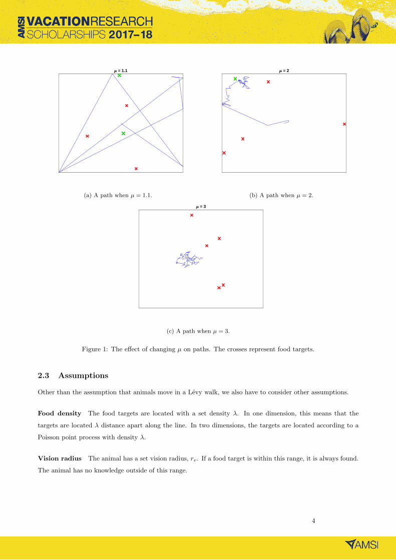
lengths, as can be seen in Figure 1 in a two-dimensional space. As µ → 1, the steps are generally larger and

it becomes like ballistic motion. As µ → 3, the steps become smaller and the path looks more like Brownian

motion.

3

= 1.1

(a) A path when µ = 1.1.

= 2

(b) A path when µ = 2.

= 3

(c) A path when µ = 3.

Figure 1: The effect of changing µ on paths. The crosses represent food targets.

2.3 Assumptions

Other than the assumption that animals move in a Levy walk, we also have to consider other assumptions.

Food density The food targets are located with a set density λ. In one dimension, this means that the

targets are located λ distance apart along the line. In two dimensions, the targets are located according to a

Poisson point process with density λ.

Vision radius The animal has a set vision radius, rv. If a food target is within this range, it is always found.

The animal has no knowledge outside of this range.

4

Memoryless The animal has no memory of previously located food targets and cannot learn the location of

a food target outside of the vision radius rv. It also has no memory of its previous search path, successful or

otherwise.

Constant Speed The animal is assumed to be moving at a constant speed, so the distance travelled is

equivalent to the time taken. Therefore, efficiency in time is equivalent to efficiency in distance.

No other factors The situation being modelled assumes no other factors such as moving food targets,

predators, physical obstacles, the animal tiring, etc.

Types of Foraging There are two types of foraging that will be considered: destructive and non-destructive.

In destructive foraging a found food target is destroyed and cannot be revisited. For non-destructive foraging,

a target may be revisited (though the model will be designed to prevent the animal continually eating a single

food target forever).

3 One-Dimensional Case

To begin analysing the stochastic optimal foraging problem, it is simpler to first consider the one-dimensional

case. In this scenario, the animal moves along a single line, with food targets located λ distance apart (see

Figure 2).

λ

Food target

x = 0 x = λ

Figure 2: The one-dimensional space in which the animal is foraging. Food targets are located λ distance apart.

The problem can be reduced to the bottom interval.

We can reduce the area of interest to a single interval of length λ (as in Figure 2). Since the animal will

always find food if it is within rv of a food target, then it is impossible for an animal to ‘jump over’ a food

target without stopping and eating it. For non-destructive foraging, the animal will therefore always be within

an interval of length λ, with the next possible food target being one of the endpoints of this interval. For

destructive foraging, it is true that once a food item is eaten, the new interval in which the animal can find food

5

will increase in size, however, the efficiency remains proportional. Since we are only concerned with maximising

efficiency, the problem can be reduced to the smaller interval.

In the different types of foraging, the starting position of the animal varies. For destructive foraging, the

animal begins in the middle of the interval since, on average, the forager ends up in the centre of the interval

after eating. For non-destructive foraging, the animal starts just outside food. To prevent the animal continually

eating at the same food target and to allow for food to regenerate, the animal is also moved just outside its

vision range of the target after it is found.

Under these conditions, the optimal value of µ for maximising efficiency is µopt → 1 for destructive foraging

and µopt = 2−(

ln λrv

)−2for non-destructive foraging [1].

3.1 Simulations in One Dimension

To do the simulations, we need to generate the random step-length variable from the Pareto distribution

(Equation (3)). This can be achieved by using the inverse transform technique. Let U be a uniform random

variable in the range [0, 1]. If X = F−1(U) then X is a random variable with the cumulative distribution

function FX(x) = F . This is because FX(a) = P (X ≤ a) = P (F−1(U) ≤ a) = P (U ≤ F (a)) = F (a).

In the case of the Pareto distribution, the inverse distribution used for sampling is

F−1(U) = `min(1− U)1

1−µ . (6)

We first run simulations of walks for a sufficient number of steps, then calculate efficiency for each of these

walks. Then we repeat simulations for each value of µ and calculate the average efficiency.

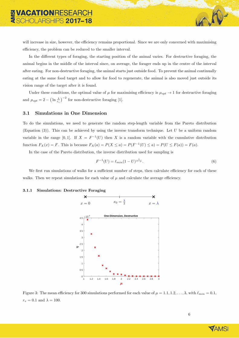
3.1.1 Simulations: Destructive Foraging

x = 0 x = λx0 = λ2

1 1.2 1.4 1.6 1.8 2 2.2 2.4 2.6 2.8 30

0.5

1

1.5

2

2.5

3

3.5

4

4.510-3 One-Dimension, Destructive

Figure 3: The mean efficiency for 300 simulations performed for each value of µ = 1.1, 1.2, . . . , 3, with `min = 0.1,

rv = 0.1 and λ = 100.

6

The optimal parameter value is µopt → 1 for destructive foraging [1]. This can be observed in the simulations

in Figure 3. As µ approaches 1, the efficiency, η, increases.

3.1.2 Simulations: Non-destructive Foraging

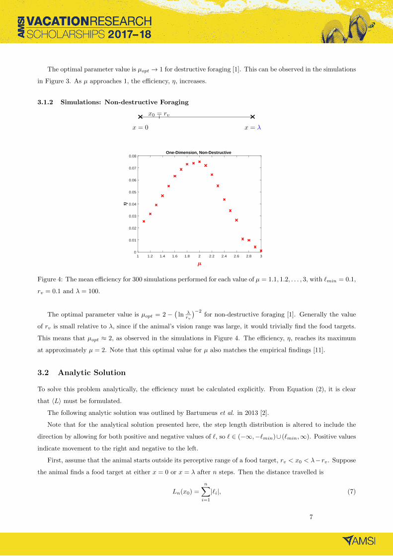
x = 0 x = λ

x0 = rv

1 1.2 1.4 1.6 1.8 2 2.2 2.4 2.6 2.8 30

0.01

0.02

0.03

0.04

0.05

0.06

0.07

0.08One-Dimension, Non-Destructive

Figure 4: The mean efficiency for 300 simulations performed for each value of µ = 1.1, 1.2, . . . , 3, with `min = 0.1,

rv = 0.1 and λ = 100.

The optimal parameter value is µopt = 2 −(

ln λrv

)−2for non-destructive foraging [1]. Generally the value

of rv is small relative to λ, since if the animal’s vision range was large, it would trivially find the food targets.

This means that µopt ≈ 2, as observed in the simulations in Figure 4. The efficiency, η, reaches its maximum

at approximately µ = 2. Note that this optimal value for µ also matches the empirical findings [11].

3.2 Analytic Solution

To solve this problem analytically, the efficiency must be calculated explicitly. From Equation (2), it is clear

that 〈L〉 must be formulated.

The following analytic solution was outlined by Bartumeus et al. in 2013 [2].

Note that for the analytical solution presented here, the step length distribution is altered to include the

direction by allowing for both positive and negative values of `, so ` ∈ (−∞,−`min)∪ (`min,∞). Positive values

indicate movement to the right and negative to the left.

First, assume that the animal starts outside its perceptive range of a food target, rv < x0 < λ− rv. Suppose

the animal finds a food target at either x = 0 or x = λ after n steps. Then the distance travelled is

Ln(x0) =

n∑i=1

|`i|, (7)

7

where `i is the length of the ith step. Since the walker is within an interval, there is a possibility of truncated

step lengths, so then each `i is dependant upon the previous position, xi−1. Then recursively, it is clear that

the total length depends on the initial position x0.

Averaging over all possible walks, we find

〈Ln〉(x0) =

n∑i=1

〈|`i|〉. (8)

Note that n can take any integer value from 1 to ∞, since it is the number of steps until a target is found.

The probability of finding a food target after n steps, Pn is dependent on n. It would be expected that after

more steps, the probability of finding a food target has increased. So, averaging over all the possible walks with

starting point x0, the average distance to finding the next food target is

〈L〉(x0) =

∞∑n=1

Pn〈Ln〉. (9)

Now, to calculate Pn, we define ρn(x) as the probability density function to find the animal between x and

x+dx after n steps. That is, it describes the probability of the animal being in each location along the interval.

Therefore, the probability that the animal has not yet discovered a food target after n steps is

P notn =

λ−rv∫rv

ρn(x)dx. (10)

Then, the complementary probability of finding a target some step n′ ≥ n+ 1 is

Pn′≥n+1 = 1− P notn . (11)

Therefore the probability of finding a food target after exactly n steps is

Pn = |Pn′≥n+1 − Pn′≥n| = |P notn − P not

n−1 |. (12)

Note that ρn−1 > ρn since the probability of finding a target increases with each step. This leads to the

formulation of Pn,

Pn =

λ−rv∫rv

[ρn−1(x)− pn(x)]dx. (13)

Combining this with Equation (9),

〈L〉(x0) =

∞∑n=1

λ−rv∫rv

[ρn−1(x)− ρn(x)]〈Ln〉(x)dx, (14)

which can be split into the two sums

〈L〉(x0) =

∞∑n=1

λ−rv∫rv

ρn−1(x)〈Ln〉(x)dx−∞∑n=1

λ−rv∫rv

ρn(x)〈Ln〉(x)dx. (15)

8

Changing the variable in the first sum to m = n−1 and adding in the n = 0 term into the second sum (note

that, by definition in Equation (8), 〈Ln=0〉 = 0), gives

〈L〉(x0) =

∞∑m=0

λ−rv∫rv

ρm(x)〈Lm+1〉(x)dx−∞∑n=0

λ−rv∫rv

ρn(x)〈Ln〉(x)dx

=

∞∑n=0

λ−rv∫rv

ρn(x)[〈Ln+1〉(x)− 〈Ln〉(x)]dx.

(16)

Using Equation (8),

〈Ln+1〉(x)− 〈Ln〉(x) =

n+1∑i=1

〈|`i|〉(x)−n∑i=1

〈|`i|〉(x)

=〈|`n+1|〉(x)

=〈|`|〉(x),

(17)

since the average step length for the (n+ 1)th step is equivalent to the average step length of any step.

Therefore, replacing this into Equation (16),

〈L〉(x0) =

∞∑n=0

λ−rv∫rv

ρn(x)〈|`|〉(x)dx. (18)

Now we need to consider the function ρn(x). By definition, ρi−1(xi−1) is the probability that the animal

is at position xi−1 in the interval after i − 1 steps.. The position of the animal at the next step is dependent

on its previous location. The probability of the animal being in position xi on the ith step, conditioned on

the previous location being xi−1, is given by p(|xi − xi−1|), the probability of a step length between these two

positions. Therefore, integrating over all the possible previous locations,

ρi(xi) =

λ−rv∫rv

ρi−1(xi−1)p(|xi − xi−1|)dxi−1. (19)

This expression can be applied recursively, to find

ρn(xn) =

λ−rv∫rv

· · ·λ−rv∫rv

ρ0(x0)

[n−1∏i=0

p(|xi+1 − xi|)dxi

]. (20)

Substituting this into Equation (18), we obtain

〈L〉(x0) =

∞∑n=0

λ−rv∫rv

λ−rv∫rv

· · ·λ−rv∫rv

ρ0(x0)

[n−1∏i=0

p(|xi+1 − xi|)dxi

] 〈|`|〉(x)dx. (21)

To simplify this form, we define the following integral operator

[L ρn](x) =

λ−rv∫rv

p(x− x′)ρn(x′)dx′, (22)

9

so that, in using Equation (19), ρn(x) = [L nρ0](x). Using this operator, Equation (21) can be rewritten as

〈L〉(x0) =

∞∑n=0

λ−rv∫rv

[L nρ0](x)〈|`|〉(x)dx. (23)

Analogous to a geometric series(∑∞

n=0 xn = 1

1−x , |x| < 1)

, we can find that

[(I −L )−1ρ0](x) =

∞∑n=0

[L nρ0](x), (24)

where I is the unitary operator such that [I ρ](x) = ρ(x). Then Equation (23) becomes

〈L〉(x0) =

∞∑n=0

λ−rv∫rv

[(I −L )−1ρ0](x)〈|`|〉(x)dx. (25)

Now note that since we assume that the initial position of the animal, x0, is fixed, then

ρ0(x) = δ(x− x0), (26)

where δ denotes the Dirac delta function:

δ(x) =

+∞, x = 0

0, x 6= 0.

(27)

Using a property of the Dirac delta function(∫∞−∞ f(x)δ(x)dx = f(0)

)leads to

〈L〉(x0) = [(I −L )−1〈|`|〉](x0). (28)

This is a closed analytical form, which can be used to calculate the efficiency for the animal’s foraging

strategy. To use Equation (28), the average step length of a single step must be calculated. The usual average

in free space is 〈|`|〉 =∫∞−∞|`|p(`)d`. However, since there is a possibility of truncation of steps due to the

presence of food targets at x = 0 and x = λ, the average step length depends on the initial position, x0, and is

given by

〈|`|〉 =

x0−`min∫rv

(x0 − x)p(|x− x0|)dx+

λ−rv∫x0+`min

(x− x0)p(|x− x0|)dx

+(x0 − rv)rv∫−∞

p(|x− x0|)dx+ (λ− rv − x0)

∞∫λ−rv

p(|x− x0|)dx,

(29)

where rv + `min ≤ x0 ≤ λ − rv − `min. The first two integrals represent a step to the left and to the right

which are not truncated and the third and fourth represent truncation due to finding a target at x = 0 and

x = λ, respectively.

One way to solve the exact formal expression in Equation (28) is to use numerical methods by approximating

the continuous interval by smaller discrete intervals (smaller than problem-relevant values rv and `min). This

10

turns the integrals into summations. Using this method, Bartumeus et al. [2] found that µopt → 1 for destructive

foraging and µopt ≈ 2 for non-destructive foraging. This agrees with the previous analytic results [1] referenced

in Section 3.1.

Note that this analytic method can also be applied to other heavy tailed distributions (exponential, bounded

Pareto, bounded exponential), but it can be shown that the Pareto distribution outperforms these others.

4 Two-Dimensional Case

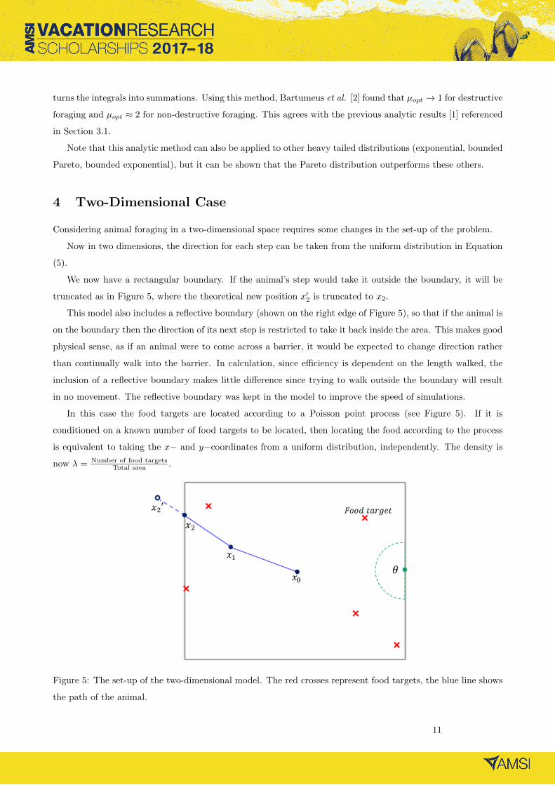
Considering animal foraging in a two-dimensional space requires some changes in the set-up of the problem.

Now in two dimensions, the direction for each step can be taken from the uniform distribution in Equation

(5).

We now have a rectangular boundary. If the animal’s step would take it outside the boundary, it will be

truncated as in Figure 5, where the theoretical new position x′2 is truncated to x2.

This model also includes a reflective boundary (shown on the right edge of Figure 5), so that if the animal is

on the boundary then the direction of its next step is restricted to take it back inside the area. This makes good

physical sense, as if an animal were to come across a barrier, it would be expected to change direction rather

than continually walk into the barrier. In calculation, since efficiency is dependent on the length walked, the

inclusion of a reflective boundary makes little difference since trying to walk outside the boundary will result

in no movement. The reflective boundary was kept in the model to improve the speed of simulations.

In this case the food targets are located according to a Poisson point process (see Figure 5). If it is

conditioned on a known number of food targets to be located, then locating the food according to the process

is equivalent to taking the x− and y−coordinates from a uniform distribution, independently. The density is

now λ = Number of food targetsTotal area .

Figure 5: The set-up of the two-dimensional model. The red crosses represent food targets, the blue line shows

the path of the animal.

11

4.1 Simulations in Two Dimensions

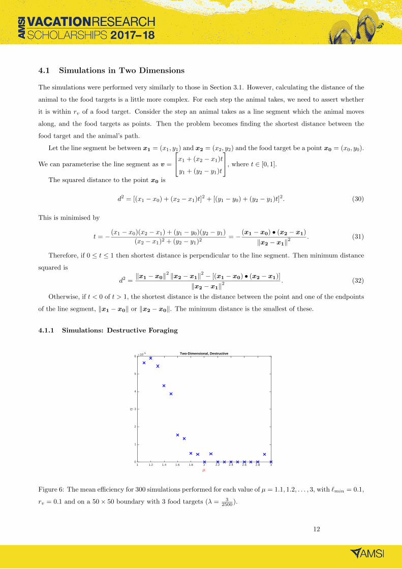
The simulations were performed very similarly to those in Section 3.1. However, calculating the distance of the

animal to the food targets is a little more complex. For each step the animal takes, we need to assert whether

it is within rv of a food target. Consider the step an animal takes as a line segment which the animal moves

along, and the food targets as points. Then the problem becomes finding the shortest distance between the

food target and the animal’s path.

Let the line segment be between x1 = (x1, y1) and x2 = (x2, y2) and the food target be a point x0 = (x0, y0).

We can parameterise the line segment as v =

x1 + (x2 − x1)t

y1 + (y2 − y1)t

, where t ∈ [0, 1].

The squared distance to the point x0 is

d2 = [(x1 − x0) + (x2 − x1)t]2 + [(y1 − y0) + (y2 − y1)t]2. (30)

This is minimised by

t = − (x1 − x0)(x2 − x1) + (y1 − y0)(y2 − y1)

(x2 − x1)2 + (y2 − y1)2= − (x1 − x0) • (x2 − x1)

‖x2 − x1‖2. (31)

Therefore, if 0 ≤ t ≤ 1 then shortest distance is perpendicular to the line segment. Then minimum distance

squared is

d2 =‖x1 − x0‖2 ‖x2 − x1‖2 − [(x1 − x0) • (x2 − x1)]

‖x2 − x1‖2. (32)

Otherwise, if t < 0 of t > 1, the shortest distance is the distance between the point and one of the endpoints

of the line segment, ‖x1 − x0‖ or ‖x2 − x0‖. The minimum distance is the smallest of these.

4.1.1 Simulations: Destructive Foraging

µ

1 1.2 1.4 1.6 1.8 2 2.2 2.4 2.6 2.8 3

η

×10 -5

0

1

2

3

4

5

6Two-Dimensional, Destructive

Figure 6: The mean efficiency for 300 simulations performed for each value of µ = 1.1, 1.2, . . . , 3, with `min = 0.1,

rv = 0.1 and on a 50× 50 boundary with 3 food targets (λ = 32500 ).

12

For destructive foraging in a two-dimensional space, the simulations (Figure 6) indicate that µopt → 1. This is

the same result as found in the one-dimensional case.

4.1.2 Simulations: Non-Destructive Foraging

µ

1 1.2 1.4 1.6 1.8 2 2.2 2.4 2.6 2.8 3

η×10 -4

2

2.5

3

3.5

4

4.5

5

5.5

6

6.5

7Two-Dimension, Non-Destructive

Figure 7: The mean efficiency for 300 simulations performed for each value of µ = 1.1, 1.2, . . . , 3, with `min = 0.1,

rv = 0.1 and on a 50× 50 boundary with 3 food targets (λ = 32500 ).

For non-destructive foraging in a two-dimensional model, the simulations in Figure 7 show that µopt → 3.

5 Conclusion

The aim of this research was to maximise the efficiency of animal foraging in order to be able to better understand

and model animal behaviour and movements. This was investigated in both the simpler one-dimensional space

and in a two-dimensional space. We also considered the differences in efficiency when assuming destructive

foraging and non-destructive foraging. We used simulations to confirm the previously reported results for the

one-dimensional case (µopt → 1 for destructive foraging and µopt = 2−(

ln λrv

)−2for non-destructive foraging).

We also analysed the theoretical solution for this problem in one dimension. Using the framework created in the

one-dimensional case, the problem was extended to two dimensions. We used simulations to find the optimal

value for µ such that efficiency is maximised (µopt → 1 for destructive foraging and µopt → 3 for non-destructive

foraging).

Further work into this area would of course include a rigorous analytic calculation of the efficiency for the

two-dimensional case.

There is still research being done on whether a Levy walk is the best model for animal foraging [10].

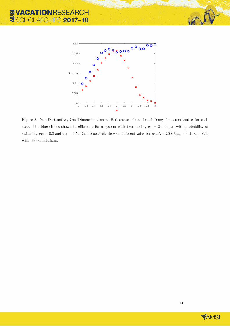
Other work in this area also indicate that a mode-switching approach leads to a higher efficiency in many

cases [9] which we investigated briefly using simulations (see Figure 8).

13

1 1.2 1.4 1.6 1.8 2 2.2 2.4 2.6 2.8 30

0.005

0.01

0.015

0.02

0.025

0.03

Figure 8: Non-Destructive, One-Dimensional case. Red crosses show the efficiency for a constant µ for each

step. The blue circles show the efficiency for a system with two modes, µ1 = 2 and µ2, with probability of

switching p12 = 0.5 and p21 = 0.5. Each blue circle shows a different value for µ2. λ = 200, `min = 0.1, rv = 0.1,

with 300 simulations.

14

References

[1] Viswanathan G. M., Buldyrev S. V., Havlin S., da Luz M. G. E., Raposo E. P., Stanley H. E. (1999).

Optimising the success of random searches. Nature 401.

[2] Bartumeus F., Raposo E.P., Viswanathan G.M., da Luz M.G.E. (2013) Stochastic Optimal Foraging The-

ory. In: Lewis M., Maini P., Petrovskii S. (eds) Dispersal, Individual Movement and Spatial Ecology.

Lecture Notes in Mathematics, vol 2071. Springer, Berlin, Heidelberg.

[3] James A., Plank J. M., Edwards A. M., (2011). Assessing Levy walks as models of animal foraging. J.R.

Soc. Interface, 8:1233-1247.

[4] Atkinson, R. P., C. J. Rhodes, D. W. Macdonald, and R. M. Anderson. 2002. Scale-free dynamics in the

movement patterns of jackals. Oikos 98:134140.

[5] Cole, B. J. 1995. Fractal time in animal behaviour: the movement activity of Drosophtla. Animal Behaviour

50: 13171324.

[6] Viswanathan, G. M., V. Afanasyev, S. V. Buldyrev, E. J. Murphy, P. A. Prince, and H. E. Stanley. 1996.

Levy flight search patterns of wandering albatrosses. Nature 381: 413415.

[7] Mrell, A., J. P. Ball, and A. Hofgaard. 2002. Foraging and movement paths of female reindeer: insights

from fractal analysis, correlated random walks, and Levy flights. Cana- dian Journal of Zoology 80:854865.

[8] Ramos-Fernndez, G., J. L. Mateos, O. Miramontes, G. Cocho, H. Larralde, and B. Ayala-Orozco. 2004.

Levy walk patterns in the foraging movements of spider monkeys (Ateles geoffroyi). Behavioral Ecology

and Sociobiology 55: 223230.

[9] Bnichou, O, Loverdo, C, Moreau, M, Voituriez, R. (2006). Two-dimensional intermittent search processes:

An alternative to Levy flight strategies. Physical review. E, Statistical, nonlinear, and soft matter physics.

74. 020102. 10.1103/PhysRevE.74.020102.

[10] Benhamou, Simon. How Many Animals Really Do the Lvy Walk? Ecology, vol. 88, no. 8, 2007, pp. 19621969.

JSTOR, JSTOR, www.jstor.org/stable/27651327.

[11] G.M. Viswanathan, E.P. Raposo, M.G.E da Luz (2008). Levy flights and superdiffusion in the context of

biological encounters and random searches. Physics of Life Reviews Volume 5, Issue 3.

15