optimal cardiovascular treatment strategies in kidney

Optimal cardiovascular treatment strategies in kidneydisease: causal inference from observational dataFu, E.L.

CitationFu, E. L. (2021, October 28). Optimal cardiovascular treatment strategies inkidney disease: causal inference from observational data. Retrieved fromhttps://hdl.handle.net/1887/3221348 Version: Publisher's Version

License:Licence agreement concerning inclusion of doctoralthesis in the Institutional Repository of the Universityof Leiden

Downloaded from: https://hdl.handle.net/1887/3221348 Note: To cite this publication please use the final published version (ifapplicable).

https://hdl.handle.net/1887/license:5



https://hdl.handle.net/1887/3221348

PART I Methodological considerations for causal inference from observational data

CHAPTER 2

Pharmacoepidemiology for nephrologists: potential biases and how to overcome them

Edouard L. Fu, Merel van Diepen, Yang Xu, Marco Trevisan, Friedo W. Dekker, Carmine Zoccali, Kitty J. Jager, Juan-Jesus Carrero

Clin Kidney J 2020; 14: 1317-1326

26

AbstractObservational pharmacoepidemiological studies using routinely collected healthcare data are increasingly being used in the field of nephrology to answer questions on the effectiveness and safety of medications. This review discusses a number of biases that may arise in such studies and proposes solutions to minimize them during the design or statistical analysis phase. We first describe designs to handle confounding by indication (e.g. active comparator design) and methods to investigate the influence of unmeasured confounding, such as the E-value, the use of negative control outcomes and control cohorts. We next discuss prevalent user and immortal time biases in pharmacoepidemiology research, and how these can be prevented by focussing on incident users and applying either landmarking, using a time-varying exposure or the cloning, censoring and weighting method. Lastly, we briefly discuss the common issues with missing data and misclassification bias. When these biases are properly accounted for, pharmacoepidemiological observational studies can provide valuable information for clinical practice.

27

CHAPTER 2 - Biases in pharmacoepidemiology

2

IntroductionPharmacoepidemiology uses epidemiological methods to study the use, therapeutic effects and risks of medications in large populations (1). Due to the availability of routinely collected healthcare data from registries, electronic health records or claims databases, observational pharmacoepidemiological studies are increasingly being used to generate evidence to inform clinical practice. Our first review discussed the scope and research questions that are studied within the field of pharmacoepidemiology, and described the strengths and caveats of the most commonly used study designs to answer such questions (2). We now focus on the most common biases that may occur when using observational data to study the causal effects of medication on health outcomes. We will attempt to offer possible solutions in the design or statistical analysis to prevent or minimize such biases. The review is intended as an introduction to the field for those who wish to critically appraise pharmacoepidemiological studies or conduct such studies.

Confounding by indicationConfounding by indication is a threat to any observational study assessing the effects of medications, since treatment is not randomly assigned to patients. Confounding by indication arises when the indications for treatment, such as age and comorbidities, are also related to the outcome under study (3). For example, treatment is generally given to those with a worse prognosis. The reverse may also occur, when newly introduced drugs are first prescribed to individuals perceived as healthier and who may be more likely to tolerate them (4). Both situations lead to an uneven distribution of prognostic factors between treatment groups, which biases a direct comparison. Take the case shown in Figure 1A, where albuminuria is a confounder for the effect of ACE inhibitor treatment on kidney replacement therapy: individuals with albuminuria are more likely to be prescribed ACE inhibitors and albuminuria is also an independent risk factor for kidney replacement therapy. Unknown or unmeasured confounders for the treatment-outcome relationship may also be present, such as smoking (if this variable has not been measured and we would assume that smoking can affect the decision to start ACE inhibitor therapy as well as the outcome).

28

Figure 1. (A) Confounding by indication arises when prognostic factors for the outcome also infl uence the

decision to start treatment. Some confounders may be measured, which can be adjusted for in the analysis,

whereas others are unmeasured, leading to residual confounding. (B) When unintended outcomes are

studied, less confounding by indication will be present. The indications for ACEi treatment likely do not

increase the risk for the outcome angioedema. (C) An ideal active comparator has similar indications as

the medication under study, thereby decreasing confounding by indication. Ideally, the active comparator

should have no infl uence on the outcome. (D) Negative control outcomes need to have similar measured

and unmeasured confounders as the treatment-outcome relationship under study. Furthermore, treatment

should not have an infl uence on the negative control outcome.

29


2

Addressing confounding by indication when designing a pharmacoepidemiological studyWhen designing observational studies to investigate medication effectiveness or safety, we should be aware that some research questions will be more susceptible to confounding than others. Confounding will generally play a larger role when studying the beneficial or “intended” effects of treatments, since the indications for treatment are very likely to be related to the prognosis of the patient (5). On the other hand, if the outcome is completely unrelated to the indications for treatment, such as when studying rare side effects or “unintended” effects, no confounding would be present (6). A classic example is the relationship between ACE inhibitors and angioedema. Patient characteristics that determine treatment status (e.g. cardiovascular risk, albuminuria, blood pressure) are unlikely to be associated with the outcome angioedema. Consequently, the arrow from treatment indication to outcome will be absent, and confounding by indication will not be an issue (Figure 1B).

Applying an active comparator design may also decrease confounding by indication (7). In an active comparator design, the medication of interest is compared with another drug that has similar indications, instead of a non-user group. The more exchangeable the active comparator is for the medication of interest, the lower the risk for potential confounding will be. After all, if both treatment groups would have identical treatment indications (both measured and unmeasured characteristics), there would be no arrow from indication to treatment and confounding by indication is removed (Figure 1C) (8). A recent example applying an active comparator design investigated whether proton pump inhibitors (PPI) increased the risk of chronic kidney disease (CKD) (9). Comparing PPI users with non-users may suffer from unmeasured confounding, since non-users are generally healthier and not all confounders may have been captured in the dataset and adjusted for. Histamine-2 receptor (H2) antagonists are prescribed for similar indications as PPI. Users of these two medications may be more similar regarding comorbidities, medication use and other unmeasured variables.

Adjusting for confounding during the statistical analysisSelecting an appropriate set of confounders to adjust for is critical when conducting pharmacoepidemiological studies (10). In general, it is not recommended to use data-driven variable selection methods to identify confounders, such as only retaining statistically significant confounders or including variables that change the regression coefficient of the treatment variable (11-13). Such data-driven approaches can lead to bias if they adjust for mediators (i.e. variables in the causal pathway between exposure and outcome) (11), colliders (e.g. a variable caused by both treatment and outcome) (14, 15) and instrumental variables (i.e. variables strongly

30

related to the exposure but not to the outcome) (16), although some sophisticated statistical covariate selection methods are currently under development (10, 17-19). Instead, we suggest to make directed acyclic graphs (DAGs) and select confounders based on subject-matter knowledge and biological plausibility (20, 21). Since DAGs rely on prior knowledge and assumed causal effects, they do not tell whether these assumptions are correct. Different researchers can have different views which factor causes the other and this may result in different choices regarding which confounders to adjust for. DAGs can aid in this discussion by making the causal assumptions explicit in a graphical manner.

Once the confounders have been selected, various methods can be used to adjust for confounding. These include, for instance, multivariable regression, standardization and propensity score methods (propensity score matching, weighting, stratification or adjustment). In the time-fixed setting (i.e. when treatment is only measured once), all methods generally suffice to adjust for measured confounding, although the interpretation of the effect estimate may differ depending on the method and some methods are preferred in specific settings (22-25). A thorough discussion on the merits and caveats of multivariable regression and propensity score methods can be found elsewhere (26). Nonetheless, in the setting of time-varying treatments (i.e. when treatment is received at multiple timepoints and changes over time) and time-varying confounding, methods based on weighting or standardization are required to give unbiased estimates if the confounders themselves are affected by treatment (27). It should be kept in mind that all statistical methods mentioned above can only adjust for measured confounders, but not for unmeasured confounders as is sometimes claimed (28), unless the unmeasured confounders are correlated with the variables that are adjusted for (29, 30).

Assessing the impact of unmeasured confounding Although the possibility of residual or unmeasured confounding in observational analyses can never be fully eliminated, a number of steps can be taken to alleviate concerns and strengthen inferences. In this section we will elaborate on conducting sensitivity analyses to obtain corrected effect estimates, calculating the E-value, and conducting negative control outcome and control group analyses.

First and foremost, as many confounders as possible need to be identified and adjusted for by using appropriate statistical methods. However, if known confounders (e.g. albuminuria or smoking) have not been measured, corrected effect estimates can be calculated in quantitative bias analyses (31-34). This requires as input the assumed association between confounder and exposure and between confounder and outcome, and the prevalence of the confounder in the population. These numbers can be based on previous studies and can be varied over a range of values

31


2

to give an indication how sensitive the estimated treatment effect is to unmeasured confounding (35). If results lead to the same conclusion over a wide range of relevant scenarios, then the plausibility of the estimated treatment effect will increase.

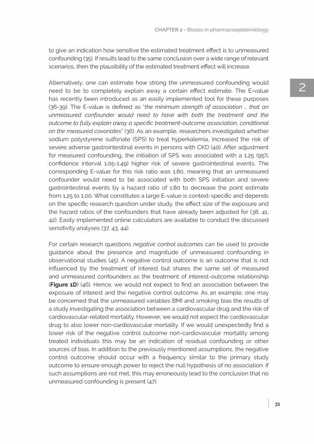
Alternatively, one can estimate how strong the unmeasured confounding would need to be to completely explain away a certain effect estimate. The E-value has recently been introduced as an easily implemented tool for these purposes (36-39). The E-value is defined as “the minimum strength of association … that an unmeasured confounder would need to have with both the treatment and the outcome to fully explain away a specific treatment-outcome association, conditional on the measured covariates” (36). As an example, researchers investigated whether sodium polystyrene sulfonate (SPS) to treat hyperkalemia, increased the risk of severe adverse gastrointestinal events in persons with CKD (40). After adjustment for measured confounding, the initiation of SPS was associated with a 1.25 (95% confidence interval 1.05-1.49) higher risk of severe gastrointestinal events. The corresponding E-value for this risk ratio was 1.80, meaning that an unmeasured confounder would need to be associated with both SPS initiation and severe gastrointestinal events by a hazard ratio of 1.80 to decrease the point estimate from 1.25 to 1.00. What constitutes a large E-value is context-specific and depends on the specific research question under study, the effect size of the exposure and the hazard ratios of the confounders that have already been adjusted for (38, 41, 42). Easily implemented online calculators are available to conduct the discussed sensitivity analyses (37, 43, 44).

For certain research questions negative control outcomes can be used to provide guidance about the presence and magnitude of unmeasured confounding in observational studies (45). A negative control outcome is an outcome that is not influenced by the treatment of interest but shares the same set of measured and unmeasured confounders as the treatment of interest-outcome relationship (Figure 1D) (46). Hence, we would not expect to find an association between the exposure of interest and the negative control outcome. As an example, one may be concerned that the unmeasured variables BMI and smoking bias the results of a study investigating the association between a cardiovascular drug and the risk of cardiovascular-related mortality. However, we would not expect the cardiovascular drug to also lower non-cardiovascular mortality. If we would unexpectedly find a lower risk of the negative control outcome non-cardiovascular mortality among treated individuals this may be an indication of residual confounding or other sources of bias. In addition to the previously mentioned assumptions, the negative control outcome should occur with a frequency similar to the primary study outcome to ensure enough power to reject the null hypothesis of no association. If such assumptions are not met, this may erroneously lead to the conclusion that no unmeasured confounding is present (47).

32

Similarly, one can test whether associations are as expected in a certain control group. The direction of the expected association (either a positive, negative or null association) can be based on physiologic mechanisms or evidence from randomized trials (48). For example, Weir et al. hypothesized that users of high-dialyzable β-blocker would have an increased risk of mortality compared with users of low-dialyzable β-blocker, due to loss of high-dialyzable β-blocker in the dialysate (49). To strengthen their inferences, a control group of patients with CKD G4-5 was constructed in whom a similar effectiveness of high-dialyzable and low-dialyzable beta-blockers was expected and subsequently demonstrated. Control groups can also strengthen inferences by showing similar results between observational studies and randomized trials. We recently evaluated the effectiveness of beta-blockers in patients with heart failure and advanced CKD, a population which was excluded from landmark heart failure trials (50). A positive control group including heart failure patients with moderate CKD showed a benefit similar to that observed in moderate CKD patients from randomized trials. This positive control analysis further supported a causal explanation for the results in the advanced CKD cohort.

Prevalent user and immortal time biasesWe now discuss two types of biases which often occur in pharmacoepidemiological studies, but that can and should be avoided by adhering to a simple principle: aligning the start of the follow-up with the start of exposure.

Prevalent user biasWhen we want to assess the effectiveness of initiating a drug, it is recommended to include incident medication users instead of prevalent users (51, 52). In a new user or incident user design, only individuals who initiate the medication of interest are studied and followed from the date of treatment initiation. Therefore, the start of follow-up and start of treatment will align, and all events that occur after drug initiation are captured (53, 54). In contrast, prevalent user designs include individuals who initiated the exposure of interest some time before the start of follow-up (Figure 2A). Comparing prevalent users to non-users may introduce selection bias since individuals who died before enrolment cannot, per definition, be included in the analysis, and events occurring shortly after drug initiation are neither observed (55, 56). To better understand why this selection bias arises, we give a real-world example. Suppose we conducted a randomized trial and found that a certain medication increased the risk of myocardial infarction with a hazard ratio of 1.24. We now reanalyze the data by starting follow-up at two years after randomization. Hence, we only count the myocardial infarctions that occurred after two years of follow-up. By doing so, we also exclude all individuals who died

33


2

or experienced myocardial infarction in the first two years after randomization. This new analysis paradoxically (rather erroneously) shows that the medication lowers the risk of myocardial infarction. Since the medication increases the risk of myocardial infarction, the treatment arm will be progressively depleted of patients most susceptible to the event (57). After two years the treated group will only consist of survivors who likely do not have other risk factors for myocardial infarction. Therefore, comparing these survivors in the treatment group with those remaining in the control group leads to an unfair advantage for the treatment group.

Figure 2. Graphical visualization of prevalent user bias (A) and immortal time bias (B) when setting up the

start of follow-up in a study. For prevalent user bias, start of follow-up occurs after treatment initiation

whereas for immortal time bias, the start of follow-up occurs before treatment initiation. These biases can

be prevented by aligning the start of follow-up with the start of exposure.

34

Prevalent user bias is one of the proposed reasons why postmenopausal hormone therapy appeared protective for coronary heart disease in observational studies, but was actually harmful when subsequent randomized trials were conducted (58, 59). Besides the fact that the effect estimates from a prevalent user design are biased, they also do not inform decision making as the decision to start the treatment was already made in the past. Studies applying a prevalent user design do not answer the relevant question whether treatment should be initiated. The results of such a study can only tell you that if a person has survived on treatment for this long, we know he is not susceptible to the event, which gives him a better prognosis than untreated individuals who are still susceptible.

Immortal time biasImmortal time bias occurs when patients are classified into treatment groups at baseline based on the treatment they take after baseline (Figure 2B) (60, 61). This leads to a period of time (i.e. immortal time) between baseline and start of treatment where no deaths can occur in the treatment group, thereby biasing results in favor of the treatment group. As an example, a pharmacoepidemiological study investigated the long-term effects of metformin use versus no metformin use on mortality and end-stage kidney disease (62). In this study, follow-up started when patients had a first creatinine measurement, but patients were classified as metformin users when they were prescribed metformin for more than 90 days during the follow-up period. Using post-baseline information on metformin use to classify patients at baseline into the metformin group leads to an unfair survival advantage for metformin users (63). Imagine that all individuals in the metformin group started medication only after 5 years of follow-up. By definition, no deaths would then occur in the metformin group during the first 5 years of follow-up. After all, individuals who have an event prior to taking up treatment would be classified as untreated. Using post-baseline information for exposure classification thus results in immortal time bias (60, 64). To what extent the effect estimate is biased depends on the total amount of follow-up that is erroneously misclassified under the metformin group. The bias will increase with a larger proportion of exposed study participants, a larger amount of time between start of follow-up and initiation of treatment and a longer duration of follow-up (65).

Potential solutions to mitigate immortal time biasWe now discuss three designs that could be applied to avoid immortal time bias: landmarking, using a time-varying exposure and using treatment strategies with grace periods. Other more complex solutions exist but are outside the scope of this review and are discussed elsewhere (66-68).

35


2

In pharmacoepidemiological studies we are often interested in the effects of initiating medication on a particular outcome after a certain event has occurred. A recent clinical example is the effect of initiating renin-angiotensin system inhibitors on mortality and recurrent AKI after acute kidney injury (AKI) (69-71). When using routinely collected healthcare data to study such questions, it is often difficult to assign individuals to the correct exposure groups: individuals become eligible for inclusion in our study immediately after the AKI event and follow-up will start at that moment. However, directly after the AKI event all individuals will likely be unexposed in our dataset, as individuals will gradually initiate therapy during follow-up. We cannot classify individuals in exposure groups based on post-baseline information as this will lead to immortal time bias. The easiest solution is then to move the baseline of our study from the date of the AKI event to a later time, e.g. 6 months after the AKI event. Our follow-up will therefore start at 6 months after the index AKI event (Figure 3) (72-74). This method is called landmarking and was recently applied by Brar et al. for this particular research question (69). In the landmarking method all individuals who died or developed the outcome between the AKI event and the newly chosen start of follow-up (i.e. 6 months after AKI) are excluded; those who initiate treatment during this period are considered exposed, and those who do not initiate treatment during this period are considered unexposed. Although landmarking prevents immortal time bias, the attentive reader will have noted that it can introduce prevalent user bias, which was discussed in the previous section.

Figure 3. Design of a landmark analysis to prevent immortal time bias. In the landmark analysis, follow-up

starts at a chosen time period after a certain event, in this example at 6 months. Hence, all individuals that

died before month 6 are excluded from the analysis (individual 4). Individuals are then classified according

to exposure status in the first 6 months. Individuals 3, 5 and 6 are therefore considered treated, whereas

individuals 1 and 2 are considered untreated.

36

The next solution that prevents immortal time bias and allows starting follow-up immediately after the event has occurred is the use of a time-varying exposure (Figure 4). When using a time-varying exposure, individuals are allowed to switch exposure status from untreated to treated at the time of treatment initiation. Hence, individuals will contribute persontime to the unexposed group before treatment initiation, and to the exposed group after treatment initiation. This ensures that the time between start of follow-up and initiation of treatment will be correctly assigned to the non-users. For example, Hsu et al. used a time-varying exposure to study the effect of RASi after AKI on the risk of recurrent AKI (70). As previously mentioned, using a time-varying exposure involves time-varying confounding. When these confounders are also influenced by prior treatment, using standard methods such as multivariable regression may not be appropriate. Instead, methods such as marginal structural models that are based on inverse probability weighting can be used (27, 75). Applying these methods, the authors found that new use of RASi therapy was not associated with an increased risk of recurrent AKI.

Figure 4. Analysis using a time-varying exposure to prevent immortal time bias. In a time-varying design

treatment status is allowed to change from unexposed to exposed at the moment of treatment initiation.

This method allows to start of follow-up directly after the event has occurred and also does not exclude

individuals. E.g., individual 1 is considered unexposed for the first 7 months of follow-up, but after 7 months

will contribute to the exposed group. In the setting of time-varying exposures, time-varying confounding

will be present too, which sometimes requires more advanced methods such as marginal structural models

to obtain unbiased effect estimates.

37


2

Lastly, we may be interested in comparing treatment strategies that include a grace period (76). For example, we could compare the strategies “initiate an ACE inhibitor within 6 months after the AKI event” versus “do not initiate an ACE inhibitor within 6 months after the AKI event”. The length of the grace period depends on what is commonly done in clinical practice. These treatment strategies with a grace period can be investigated by using a three-step method based on cloning, censoring and weighting (Figure 5).

Figure 5. Design of a study using treatment strategies with a grace period based on cloning, censoring and

weighting. Another method is comparing treatment strategies that include a grace period. Each individual

is duplicated and assigned to one of two treatment strategies. In this example, clones 1a to 6a follow the

strategy “initiate ACEi within 6 months”, whereas clones 1b to 6b follow the strategy “do not initiate ACEi

within 6 months”. Note that copies 1a and 1b represent the same individual. Since copy 1a is assigned to

initiating within 6 months, he is censored after month 6 as he did not initiate treatment. The censoring is

likely to be informative and inverse probability weighting is required to adjust for this.

38

Briefly, each individual is duplicated so that there are two copies of each individual in the dataset. Each copy is then assigned to one of the treatment strategies. In the second step the copies are censored if and when their observed treatment does not adhere anymore to their assigned treatment strategy. Since this censoring is likely to be informative, the third step applies inverse probability weighting to correct for this. Bootstrapping can be used to take into account the cloning and weighting and obtain valid confidence intervals. An advantage of using treatment strategies with grace periods is that a wide range of questions can be answered, including questions on the duration of treatment and dynamic treatment strategies (e.g., when should treatment be initiated) (76, 77). However, this method requires that detailed longitudinal data is present to adequately adjust for the informative censoring. The three methods of landmarking, time-varying exposure and treatment strategies with grace periods are contrasted in Table 1 and graphically depicted in Figures 3-5.

Table 1. Different methods to address immortal time bias in pharmacoepidemiological analyses.

Landmark analysis Time-varying exposure

Cloning, censoring and weighting

Immortal time bias No No No

Start of follow-up At landmark At event At event

Causal effect Initiating versus not initiating at x months after event (landmark), conditional on having survived until landmark†

Initiating and always using versus never using (marginal structural model)

Initiating within x months versus not initiating within x months after event

Prevalent user bias Possible No No

Results apply to Individuals surviving until landmark

All individuals All individuals

Baseline confounding Yes Yes No*

Time-varying exposure No Yes No

Time-varying confounding

No Yes No

Informative censoring No No Yes

G-methods§ required No Sometimes (if confounder is influenced by prior treatment)

Yes (inverse probability weighting)

† This is often how the effect estimate from a landmark analysis is interpreted. However, the landmark

analysis conditions on surviving until a certain timepoint and classifies individuals into treatment groups

based on past information, thereby possibly introducing prevalent user bias. * Due to the cloning, at baseline each individual will appear in both treatment arms. Hence, no baseline

confounding will be present.§ Methods based on standardization or inverse probability weighting, such as the G-formula or marginal

structural models.

39


2

Missing data and misclassificationWe now briefly discuss the implications of missing data and misclassification for bias and possible solutions. Although these two sources of bias are a common issue in pharmacoepidemiological studies, they are often less emphasized compared with confounding.

Missing dataWe usually aim to adjust for as many confounders as possible in our analysis, including available laboratory tests (e.g. albuminuria, potassium) and clinical variables (e.g. blood pressure, BMI) which are indications for treatment. However, it is not unusual that a large proportion of these values are missing in routinely collected data. For example, in an analysis using data from the Swedish Renal Registry, baseline potassium and albuminuria-to-creatinine-ratio measurements were missing in 32% and 41% of patients, respectively (78). In such situations, researchers often perform a complete case analysis by restricting to individuals with both measurements available. However, this may lead to a drastic reduction in power and often also bias (79, 80). Methods such as multiple imputation are therefore recommended and are available in most software packages. These methods can reduce these biases even with large proportions of missing data (up to 90%) if data are missing at random or missing completely at random, sufficient auxiliary information is available and the imputation model is properly specified (81). It is therefore important to discuss the reasons for missingness and the plausibility of the missing at random assumption. In the above example, the researchers explained that although albuminuria and potassium values were measured in clinical practice, they were not among the list of mandatory laboratory markers that needed to be reported to the Swedish Renal Registry. Thus, some clinicians took the time to report those lab tests and others not, a decision that could be assumed to be at random. Furthermore, the authors showed that clinical characteristics were similar for individuals with and without missing data, thereby making the missing at random assumption plausible. More information on the different types of missingness (79, 80), in what situations complete case analysis leads to unbiased results (82), as well as tutorials to implement multiple imputation can be found elsewhere (83).

MisclassificationAlthough misclassification will be present in nearly every study, it may be especially important when using routinely collected healthcare data (84). Misclassification may for instance occur when using ICD-10 codes to ascertain the occurrence of chronic kidney disease or acute kidney injury, as these are not always coded in clinical practice and many patients are unaware of their disease (85-87). When AKI

40

diagnosis based on ICD coding is used as an outcome, differential misclassification will arise when doctors are more aware or more likely to encode AKI if certain drugs are prescribed. Basing kidney outcomes on biochemical criteria may sometimes mitigate such biases, but can also introduce bias when creatinine testing is more often directed towards sicker patients or patients at risk of CKD progression. Misclassification of comorbidities may be a significant concern in routinely collected data since the absence of a diagnosis (recording) is often considered to indicate absence of the comorbidity. Residual confounding may occur when confounders are misclassified and the direction can be both away or toward a null effect (84). Misclassification influences study results in ways that are often not anticipated, and simple heuristics about the impact of misclassification (towards the null or not) are often incorrect (88, 89). Many correction methods for misclassification exist, but these require information about its magnitude and structure (i.e. dependent, non-dependent, differential, non-differential) (90-93). As such information is often not available in electronic databases, sensitivity analyses similar to those for unmeasured confounding can be performed to estimate the influence of misclassification on results (33, 94).

ConclusionPharmacoepidemiological studies are increasingly being used to answer causal questions on the effectiveness and safety of medications in order to inform clinical decision making. In this review we discussed the most important biases that commonly occur in such studies. We also reviewed methods to account for these biases, which are summarized in Table 2. Researchers can and should prevent problems arising from immortal time and prevalent user biases in their study design. Confounding by indication bias can be tackled by using an active comparator design and adequately adjusting for confounders. When concerns remain about confounding or misclassification, quantifying their impact on effect estimates is recommended. When these principles are correctly applied, pharmacoepidemiological observational studies can provide valuable information for clinical practice.

41


2

Table 2. Potential biases in pharmacoepidemiological studies and proposed solutions.

Potential biases

Example of how biases may arise

Possible solutions and recommendations

Confounding by indication

• Confounding by indication arises when prognostic factors for the outcome are also an indication for initiating treatment.

• Unmeasured/residual confounding arises when confounders are not adjusted for, either if they are not measured in the dataset or if they are unknown.

• Time-varying confounding occurs when investigating time-varying exposures. When the confounder is influenced by past treatment, conventional methods to control for confounding will be biased.

• Research question: Unintended medication effects (e.g. rare side effects) may be less susceptible to confounding by indication than intended medication effects.

• Design: Active comparator designs may decrease confounding bias if medication is given for similar indications.

• Statistical methods: Multivariable regression, standardization or propensity score methods (matching, weighting, stratification, adjustment) can be used to control for measured confounding. Propensity score methods may have a number of advantages compared with regression, such as the ability to check if balance in confounders has been achieved. In the presence of time-varying confounding that are influenced by treatment, conventional methods lead to bias and the so called G-methods are required.

• After analysis: The impact of unmeasured confounding on effect estimates can be investigated in simulation analyses. Negative control outcomes may investigate whether unmeasured confounders bias effect estimates.

Prevalent user bias

Comparing ever users vs. never users. Including individuals after they initiate treatment will miss early outcome events and exclude those that died (depletion of susceptibles).

• Prevalent user bias can and should be prevented by aligning initiation of treatment with start of follow-up; include new users of treatment.

• Exclude prevalent users, e.g. those with drug prescription in 12 months prior to inclusion.

Immortal time bias

Classifying individuals in treatment groups based on future information not present at the start of follow-up. A period of time is created for the treated group during which the outcome cannot occur.

• Immortal time bias can and should be prevented by aligning initiation of treatment with start of follow-up. Do not use information after start of follow-up to classify individuals into exposure groups.

• Landmarking, time-varying exposure, and the cloning, censoring and weighting method.

Missing data Routinely collected healthcare data are prone to missing data. In multivariable analyses individuals with missing confounder data will be excluded. Complete case analysis often lead to bias when data is not missing completely at random, but a number of exceptions exist.

• Multiple imputation can be used to decrease bias and increase precision, even with large proportions of missing data (up to 90%) if data are missing at random or missing completely at random and the imputation model is properly specified.

• Discuss the missing data mechanism and the plausibility of the missing (completely) at random assumption.

Misclassification • Misclassification of the outcome may occur when outcomes are differentially ascertained depending on treatment status.

• Misclassification of confounders may lead to residual confounding.

• The impact of misclassification on the estimated effect size can be quantified in sensitivity analyses. Online tools are available to implement these methods.

• When external data are available, regression calibration, multiple imputation for measurement error or propensity score calibration can be used.

42

References

1. Begaud B. Dictionary of pharmacoepidemiology: Wiley, 2000.

2. Trevisan M, Fu EL, Xu Y, Jager KJ, Zoccali C, Dekker FW, et al. Pharmacoepidemiology for

nephrologists (part one): Concept, applications and considerations for study design. Clinical

Kidney Journal. 2020.

3. Kyriacou DN, Lewis RJ. Confounding by Indication in Clinical Research. JAMA. 2016;316(17):1818-9.

4. Sorensen R, Gislason G, Torp-Pedersen C, Olesen JB, Fosbol EL, Hvidtfeldt MW, et al. Dabigatran

use in Danish atrial fibrillation patients in 2011: a nationwide study. BMJ Open. 2013;3(5).

5. Vandenbroucke JP. Observational research, randomised trials, and two views of medical science.

PLoS Med. 2008;5(3):e67.

6. Bosdriesz JR, Stel VS, van Diepen M, Meuleman Y, Dekker FW, Zoccali C, et al. Evidence-based

medicine-When observational studies are better than randomized controlled trials. Nephrology

(Carlton). 2020:e13742.

7. Yoshida K, Solomon DH, Kim SC. Active-comparator design and new-user design in observational

studies. Nat Rev Rheumatol. 2015;11(7):437-41.

8. Lund JL, Richardson DB, Sturmer T. The active comparator, new user study design in

pharmacoepidemiology: historical foundations and contemporary application. Curr Epidemiol

Rep. 2015;2(4):221-8.

9. Klatte DCF, Gasparini A, Xu H, de Deco P, Trevisan M, Johansson ALV, et al. Association Between

Proton Pump Inhibitor Use and Risk of Progression of Chronic Kidney Disease. Gastroenterology.

2017;153(3):702-10.

10. VanderWeele TJ. Principles of confounder selection. Eur J Epidemiol. 2019;34(3):211-9.

11. Lederer DJ, Bell SC, Branson RD, Chalmers JD, Marshall R, Maslove DM, et al. Control of

Confounding and Reporting of Results in Causal Inference Studies. Guidance for Authors from

Editors of Respiratory, Sleep, and Critical Care Journals. Ann Am Thorac Soc. 2019;16(1):22-8.

12. Hernan MA, Hernandez-Diaz S, Werler MM, Mitchell AA. Causal knowledge as a prerequisite

for confounding evaluation: an application to birth defects epidemiology. Am J Epidemiol.

2002;155(2):176-84.

13. Robins JM. Data, design, and background knowledge in etiologic inference. Epidemiology.

2001;12(3):313-20.

14. Hernan MA, Hernandez-Diaz S, Robins JM. A structural approach to selection bias. Epidemiology.

2004;15(5):615-25.

15. Cole SR, Platt RW, Schisterman EF, Chu H, Westreich D, Richardson D, et al. Illustrating bias due

to conditioning on a collider. Int J Epidemiol. 2010;39(2):417-20.

16. Myers JA, Rassen JA, Gagne JJ, Huybrechts KF, Schneeweiss S, Rothman KJ, et al. Effects of

adjusting for instrumental variables on bias and precision of effect estimates. Am J Epidemiol.

2011;174(11):1213-22.

17. Blakely T, Lynch J, Simons K, Bentley R, Rose S. Reflection on modern methods: when worlds

collide-prediction, machine learning and causal inference. Int J Epidemiol. 2019.

18. Schneeweiss S, Rassen JA, Glynn RJ, Avorn J, Mogun H, Brookhart MA. High-dimensional

propensity score adjustment in studies of treatment effects using health care claims data.

Epidemiology. 2009;20(4):512-22.

43


2

19. Schuler MS, Rose S. Targeted Maximum Likelihood Estimation for Causal Inference in

Observational Studies. Am J Epidemiol. 2017;185(1):65-73.

20. Suttorp MM, Siegerink B, Jager KJ, Zoccali C, Dekker FW. Graphical presentation of confounding

in directed acyclic graphs. Nephrol Dial Transplant. 2015;30(9):1418-23.

21. Ferguson KD, McCann M, Katikireddi SV, Thomson H, Green MJ, Smith DJ, et al. Evidence

synthesis for constructing directed acyclic graphs (ESC-DAGs): a novel and systematic method

for building directed acyclic graphs. Int J Epidemiol. 2019.

22. Austin PC. An Introduction to Propensity Score Methods for Reducing the Effects of Confounding

in Observational Studies. Multivariate Behav Res. 2011;46(3):399-424.

23. Desai RJ, Franklin JM. Alternative approaches for confounding adjustment in observational studies

using weighting based on the propensity score: a primer for practitioners. BMJ. 2019;367:l5657.

24. Shah BR, Laupacis A, Hux JE, Austin PC. Propensity score methods gave similar results to

traditional regression modeling in observational studies: a systematic review. J Clin Epidemiol.

2005;58(6):550-9.

25. Sturmer T, Joshi M, Glynn RJ, Avorn J, Rothman KJ, Schneeweiss S. A review of the application

of propensity score methods yielded increasing use, advantages in specific settings, but not

substantially different estimates compared with conventional multivariable methods. J Clin

Epidemiol. 2006;59(5):437-47.

26. Fu EL, Groenwold RHH, Zoccali C, Jager KJ, van Diepen M, Dekker FW. Merits and caveats of

propensity scores to adjust for confounding. Nephrol Dial Transplant. 2019;34(10):1629-35.

27. Williamson T, Ravani P. Marginal structural models in clinical research: when and how to use

them? Nephrol Dial Transplant. 2017;32(suppl_2):ii84-ii90.

28. Dekkers IA, van der Molen AJ. Propensity Score Matching as a Substitute for Randomized

Controlled Trials on Acute Kidney Injury After Contrast Media Administration: A Systematic

Review. AJR Am J Roentgenol. 2018;211(4):822-6.

29. Groenwold RH, Sterne JA, Lawlor DA, Moons KG, Hoes AW, Tilling K. Sensitivity analysis for the

effects of multiple unmeasured confounders. Ann Epidemiol. 2016;26(9):605-11.

30. Patorno E, Schneeweiss S, Gopalakrishnan C, Martin D, Franklin JM. Using Real-World Data to

Predict Findings of an Ongoing Phase IV Cardiovascular Outcome Trial: Cardiovascular Safety of

Linagliptin Versus Glimepiride. Diabetes Care. 2019;42(12):2204-10.

31. Schneeweiss S. Sensitivity analysis and external adjustment for unmeasured confounders in

epidemiologic database studies of therapeutics. Pharmacoepidemiol Drug Saf. 2006;15(5):291-303.

32. Greenland S. Basic methods for sensitivity analysis of biases. Int J Epidemiol. 1996;25(6):1107-16.

33. Lash TL, Fox MP, Fink AK. Applying quantitative bias analysis to epidemiologic data. Springer.

2009.

34. Uddin MJ, Groenwold RH, Ali MS, de Boer A, Roes KC, Chowdhury MA, et al. Methods to

control for unmeasured confounding in pharmacoepidemiology: an overview. Int J Clin Pharm.

2016;38(3):714-23.

35. Groenwold RH, Nelson DB, Nichol KL, Hoes AW, Hak E. Sensitivity analyses to estimate the potential

impact of unmeasured confounding in causal research. Int J Epidemiol. 2010;39(1):107-17.

36. VanderWeele TJ, Ding P. Sensitivity Analysis in Observational Research: Introducing the E-Value.

Ann Intern Med. 2017;167(4):268-74.

37. https://www.evalue-calculator.com/.

44

38. VanderWeele TJ, Ding P, Mathur MB. Technical Considerations in the Use of the E-Value. Journal

of Causal Inference. 2019;7(2).

39. Trinquart L, Erlinger AL, Petersen JM, Fox M, Galea S. Applying the E Value to Assess the

Robustness of Epidemiologic Fields of Inquiry to Unmeasured Confounding. Am J Epidemiol.

2019;188(6):1174-80.

40. Laureati P, Xu Y, Trevisan M, Schalin L, Mariani I, Bellocco R, et al. Initiation of sodium polystyrene

sulphonate and the risk of gastrointestinal adverse events in advanced chronic kidney disease: a

nationwide study. Nephrol Dial Transplant. 2019.

41. Ioannidis JPA, Tan YJ, Blum MR. Limitations and Misinterpretations of E-Values for Sensitivity

Analyses of Observational Studies. Ann Intern Med. 2019;170(2):108-11.

42. VanderWeele TJ, Mathur MB, Ding P. Correcting Misinterpretations of the E-Value. Ann Intern

Med. 2019;170(2):131-2.

43. http://www.drugepi.org/dope-downloads/#Sensitivity%20Analysis.

44. https://sites.google.com/site/biasanalysis/.

45. Lipsitch M, Tchetgen Tchetgen E, Cohen T. Negative controls: a tool for detecting confounding

and bias in observational studies. Epidemiology. 2010;21(3):383-8.

46. Arnold BF, Ercumen A. Negative Control Outcomes: A Tool to Detect Bias in Randomized Trials.

JAMA. 2016;316(24):2597-8.

47. Groenwold RH. Falsification end points for observational studies. JAMA. 2013;309(17):1769-70.

48. Edner M, Benson L, Dahlstrom U, Lund LH. Association between renin-angiotensin system

antagonist use and mortality in heart failure with severe renal insufficiency: a prospective

propensity score-matched cohort study. Eur Heart J. 2015;36(34):2318-26.

49. Weir MA, Dixon SN, Fleet JL, Roberts MA, Hackam DG, Oliver MJ, et al. beta-Blocker dialyzability

and mortality in older patients receiving hemodialysis. J Am Soc Nephrol. 2015;26(4):987-96.

50. Fu EL, Uijl A, Dekker FW, Lund LH, Savarese G, Carrero JJ. Association between β-blocker use

and mortality/morbidity in patients with heart failure with reduced, midrange and preserved

ejection fraction and advanced chronic kidney disease. Circ Heart Fail.

51. Ray WA. Evaluating medication effects outside of clinical trials: new-user designs. Am J Epidemiol.

2003;158(9):915-20.

52. Johnson ES, Bartman BA, Briesacher BA, Fleming NS, Gerhard T, Kornegay CJ, et al. The incident

user design in comparative effectiveness research. Pharmacoepidemiol Drug Saf. 2013;22(1):1-6.

53. Hernan MA, Robins JM. Using Big Data to Emulate a Target Trial When a Randomized Trial Is Not

Available. Am J Epidemiol. 2016;183(8):758-64.

54. Hernan MA, Sauer BC, Hernandez-Diaz S, Platt R, Shrier I. Specifying a target trial prevents

immortal time bias and other self-inflicted injuries in observational analyses. J Clin Epidemiol.

2016;79:70-5.

55. Tomlinson L, Smeeth L. Angiotensin-converting enzyme inhibitor or angiotensin receptor blocker

use and renal outcomes: prevalent user designs may overestimate benefit. JAMA Intern Med.

2014;174(10):1706.

56. Stovitz SD, Banack HR, Kaufman JS. 'Depletion of the susceptibles' taught through a story, a table

and basic arithmetic. BMJ Evid Based Med. 2018;23(5):199.

57. Lajous M, Banack HR, Kaufman JS, Hernan MA. Should patients with chronic disease be told to

gain weight? The obesity paradox and selection bias. Am J Med. 2015;128(4):334-6.

45


2

58. Hernan MA, Alonso A, Logan R, Grodstein F, Michels KB, Willett WC, et al. Observational studies

analyzed like randomized experiments: an application to postmenopausal hormone therapy and

coronary heart disease. Epidemiology. 2008;19(6):766-79.

59. Dickerman BA, Garcia-Albeniz X, Logan RW, Denaxas S, Hernan MA. Avoidable flaws in

observational analyses: an application to statins and cancer. Nat Med. 2019;25(10):1601-6.

60. Suissa S. Immortal time bias in pharmaco-epidemiology. Am J Epidemiol. 2008;167(4):492-9.

61. Levesque LE, Hanley JA, Kezouh A, Suissa S. Problem of immortal time bias in cohort studies:

example using statins for preventing progression of diabetes. BMJ. 2010;340:b5087.

62. Kwon S, Kim YC, Park JY, Lee J, An JN, Kim CT, et al. The Long-term Effects of Metformin on

Patients With Type 2 Diabetic Kidney Disease. Diabetes Care. 2020;43(5):948-55.

63. Fu EL, Van Diepen M. Comment on Kwon et al. The Long-term Effects of Metformin on Patients

With Type 2 Diabetic Kidney Disease. Diabetes Care 2020;43:948-955 Diabetes Care. 2020.

64. Suissa S. Immortal time bias in observational studies of drug effects. Pharmacoepidemiol Drug

Saf. 2007;16(3):241-9.

65. Harding BN, Weiss NS. Immortal Time Bias: What Are the Determinants of Its Magnitude? Am J

Epidemiol. 2019.

66. Danaei G, Rodriguez LA, Cantero OF, Logan R, Hernan MA. Observational data for comparative

effectiveness research: an emulation of randomised trials of statins and primary prevention of

coronary heart disease. Stat Methods Med Res. 2013;22(1):70-96.

67. Karim ME, Gustafson P, Petkau J, Tremlett H, Long-Term B, Adverse Effects of Beta-Interferon for

Multiple Sclerosis Study G. Comparison of Statistical Approaches for Dealing With Immortal Time

Bias in Drug Effectiveness Studies. Am J Epidemiol. 2016;184(4):325-35.

68. Gran JM, Roysland K, Wolbers M, Didelez V, Sterne JA, Ledergerber B, et al. A sequential Cox

approach for estimating the causal effect of treatment in the presence of time-dependent

confounding applied to data from the Swiss HIV Cohort Study. Stat Med. 2010;29(26):2757-68.

69. Brar S, Ye F, James MT, Hemmelgarn B, Klarenbach S, Pannu N, et al. Association of Angiotensin-

Converting Enzyme Inhibitor or Angiotensin Receptor Blocker Use With Outcomes After Acute

Kidney Injury. JAMA Intern Med. 2018;178(12):1681-90.

70. Hsu CY, Liu KD, Yang J, Glidden DV, Tan TC, Pravoverov L, et al. Renin-Angiotensin System

Blockade after Acute Kidney Injury (AKI) and Risk of Recurrent AKI. Clin J Am Soc Nephrol.

2020;15(1):26-34.

71. Siew ED, Parr SK, Abdel-Kader K, Perkins AM, Greevy RA, Jr., Vincz AJ, et al. Renin-angiotensin

aldosterone inhibitor use at hospital discharge among patients with moderate to severe acute

kidney injury and its association with recurrent acute kidney injury and mortality. Kidney Int. 2020.

72. Dafni U. Landmark analysis at the 25-year landmark point. Circ Cardiovasc Qual Outcomes.

2011;4(3):363-71.

73. Mi X, Hammill BG, Curtis LH, Lai EC, Setoguchi S. Use of the landmark method to address

immortal person-time bias in comparative effectiveness research: a simulation study. Stat Med.

2016;35(26):4824-36.

74. Gleiss A, Oberbauer R, Heinze G. An unjustified benefit: immortal time bias in the analysis of time-

dependent events. Transpl Int. 2018;31(2):125-30.

75. Daniel RM, Cousens SN, De Stavola BL, Kenward MG, Sterne JA. Methods for dealing with time-

dependent confounding. Stat Med. 2013;32(9):1584-618.

46

76. Hernan MA, Lanoy E, Costagliola D, Robins JM. Comparison of dynamic treatment regimes via inverse probability weighting. Basic Clin Pharmacol Toxicol. 2006;98(3):237-42.

77. Cain LE, Robins JM, Lanoy E, Logan R, Costagliola D, Hernan MA. When to start treatment? A systematic approach to the comparison of dynamic regimes using observational data. Int J Biostat. 2010;6(2):Article 18.

78. Fu EL, Clase CM, Evans M, Lindholm B, Rotmans JI, van Diepen M, et al. Comparative effectiveness of renin-angiotensin system inhibitors and calcium channel blockers in individuals with advanced chronic kidney disease: a nationwide observational cohort study. Submitted. 2020.

79. de Goeij MC, van Diepen M, Jager KJ, Tripepi G, Zoccali C, Dekker FW. Multiple imputation: dealing with missing data. Nephrol Dial Transplant. 2013;28(10):2415-20.

80. Sterne JA, White IR, Carlin JB, Spratt M, Royston P, Kenward MG, et al. Multiple imputation for missing data in epidemiological and clinical research: potential and pitfalls. BMJ. 2009;338:b2393.

81. Madley-Dowd P, Hughes R, Tilling K, Heron J. The proportion of missing data should not be used to guide decisions on multiple imputation. J Clin Epidemiol. 2019;110:63-73.

82. Hughes RA, Heron J, Sterne JAC, Tilling K. Accounting for missing data in statistical analyses: multiple imputation is not always the answer. Int J Epidemiol. 2019;48(4):1294-304.

83. Blazek K, van Zwieten A, Saglimbene V, Teixeira-Pinto A. A practical guide to multiple imputation of missing data in nephrology. Kidney Int. 2020.

84. Funk MJ, Landi SN. Misclassification in administrative claims data: quantifying the impact on treatment effect estimates. Curr Epidemiol Rep. 2014;1(4):175-85.

85. Gasparini A, Evans M, Coresh J, Grams ME, Norin O, Qureshi AR, et al. Prevalence and recognition of chronic kidney disease in Stockholm healthcare. Nephrol Dial Transplant. 2016;31(12):2086-94.

86. McDonald HI, Shaw C, Thomas SL, Mansfield KE, Tomlinson LA, Nitsch D. Methodological challenges when carrying out research on CKD and AKI using routine electronic health records. Kidney Int. 2016;90(5):943-9.

87. Tomlinson LA, Riding AM, Payne RA, Abel GA, Tomson CR, Wilkinson IB, et al. The accuracy of diagnostic coding for acute kidney injury in England - a single centre study. BMC Nephrol. 2013;14:58.

88. van Smeden M, Lash TL, Groenwold RHH. Reflection on modern methods: five myths about measurement error in epidemiological research. Int J Epidemiol. 2020;49(1):338-47.

89. Jurek AM, Greenland S, Maldonado G, Church TR. Proper interpretation of non-differential misclassification effects: expectations vs observations. Int J Epidemiol. 2005;34(3):680-7.

90. Sturmer T, Schneeweiss S, Avorn J, Glynn RJ. Adjusting effect estimates for unmeasured confounding with validation data using propensity score calibration. Am J Epidemiol. 2005;162(3):279-89.

91. Cole SR, Chu H, Greenland S. Multiple-imputation for measurement-error correction. Int J Epidemiol. 2006;35(4):1074-81.

92. Spiegelman D, McDermott A, Rosner B. Regression calibration method for correcting measurement-error bias in nutritional epidemiology. Am J Clin Nutr. 1997;65(4 Suppl):1179S-86S.

93. Bang H, Chiu YL, Kaufman JS, Patel MD, Heiss G, Rose KM. Bias Correction Methods for Misclassified Covariates in the Cox Model: comparison offive correction methods by simulation and data analysis. J Stat Theory Pract. 2013;7(2):381-400.

94. Fox MP, Lash TL, Greenland S. A method to automate probabilistic sensitivity analyses of misclassified binary variables. Int J Epidemiol. 2005;34(6):1370-6.

47


2

optimal cardiovascular treatment strategies in kidney

Documents