optimal control aspects of left ventricular ejection dynamicsoda/contents/01matem%e1tic… · ·...

.I. theor. Biol. (1976) 63, 275-309

Optimal Control Aspects of Left Ventricular Ejection Dynamics

ERIK J. Nor>ws

.-lutomatic Control Laboratory, Unil>ersitJ? of Ghent, Belgium

(Received 25 June 1975, and in reaised form 27 October 1975)

A model of the ejecting left ventricle is developed in which ventricular elastance as a function of time is optimized with respect to a simple performance index selected on an energetic basis. The model correctly predicts a number of well known experimental findings concerning the effects of preload and afterload conditions and varying system parameters on left ventricular pressure and elastance waveforms and on the ejection period. The results characterize ventricular systolic elastance as dependent on both end-diastolic volume and mean aortic pressure.

1. Introduction

The dynamic performance of the left ventricle during systole has been analysed in numerous papers. One approach that has frequently been used. characterizes the ventricle in terms of the elastance function E(t) defined b>

E(t) = /qt)/V(t). (1)

P(t) and k’(t) representing the instantaneous values of left ventricular pressure and volume. Several systolic time courses of E(t) have been proposed in the literature, some being chosen for their simplicity (Warner, 1965; Defares. Hara, Osborn & McLeod, 1963; Beneken, 1964), others being calculated from physiological data (Greene, Clark, Mohr & Bourland, 1973; Suga, 1971). Ventricular performance measurements on dogs by Suga (1969, 1970), result in elastance curves that are essentially unaffected by changes in either left ventricular end-diastolic volume V,, or arterial loading conditions. Other studies however (Greene et al.. 1973 ; Taylor, Cove11 & Ross, 1969) characterize ventricular elastance as dependent on end-diastolic volume.

This paper tries to approach the problem of developing a ventricular pumping model, and determining E(t), relying on optimization aspects in biological control theory. The relevance of the optimization concept, and supporting evidence for it, have been examined in detail by Milsum (1968): loosely speaking, it is assumed that a selective survival advantage is gained

I’, 13. 17 IX

E. J. NOLDUS

by those organisms whose subsystems operate in an optimal fashion on some energetic and/or informational basis, and that as a result living systems have evolved towards optimal performance when executing a given task. Although it is by no means clear what performance criteria are relevant for biological systems, optimization seems to be a worthwhile viewpoint both for theoretical analysis, as for suggesting new experiments.

Specifically, in the present problem, our aim is to apply dynamic optimization theory to the mechanism of ventricular ejection, in order to determine which is the best force-developing strategy to eject a given volume of blood out of the ventricle. To this end the ventricular pressure P(f) during ejection, which acts as an external driving force on the system under analysis. will be optimized on the basis of a reasonable performance index related to the energy expenditure of the working ventricle. We then wish to examine how the results of this optimal strategy differ from the established facts concerning, for example, the responses of the ventricle to different types of loading conditions. If the obtained results are at least qualitatively consistent with the system’s actual behaviour, then the approach may reveal some new insights in this behaviour, and in the system’s properties when performing under varying internal and external circumstances. It will be shown that computed pressure and elastance curves bear good resemblance to measured data and that calculated and experimental results display similar tendencies when certain parameters are changed, such as average aorlic pressure, end-diastolic volume, and the parameters characterizing load dynamics. This suggests that the hypotheses formulated in the performance index may to some extent express basic principles which determine the operation of the ventricle. In this way an ejection model is obtained, based on a new, rational fundamental philosophy, which to some extent may provide a logical explanation why the ventricle operates in a specific way under given working conditions. A model of this type may predict on a rational basis how the system will react to various external perturbations, internal parameter variations, and even to internal structural changes, fat example as a result of accident or illness.

2. Problem Statement

To analyse the circulatory effects of left ventricular pumping, models of the ventricle itself, and of the arterial system must be defined. Figure 1 shows an electrical analogue of a model, similar to the ones proposed by Suga (1971). The model is quite elementary, but since we are mainly interested in investigating the system’s qualitative behaviour, and the general shapes and tendencies of waveforms, it will suit our purpose. The same model. or

LLFI‘ VENTRICULAK I:JLC I ION Dk N.(.hlt(‘S 177

I -.. E(f)

*--- Ventricular elastance ‘~l~~~:lhss?cl 1013

FIG. 1. Electrical equivalent of the pumping model under inj:cstigation.

slightly diRerent versions of it, have been used by many investigators. F‘or :t discussion, see the review by Noordergraaf (I 969) on the subject. The model’> dynamic equations are

V(t) = 1; - .!, i(0) dU (?a)

di(l) P(f) = P,(f)-I-ri(t)+L dt (2bi

I’,(f) reprexenls the aorlic blood pressure, i(t) the blood flow ralc e.jectcd o:~t of the ventricle, P the aortic valvular resistance. and L the blood inertia. /Z and C are the peripheral resistance and compliance of a lumped arterial Windkessel load. In the right hand side of equation (?a), the first term I,, represents the ventricular volume at the beginning of ejection, while 11x second term is the blood voiume ejected out of the ventricle during the time interval (0, t). Equation (2b) states that the ventricular pressure equals the sum of aortic pressure, the pressure drop across the aortic valve, \vhich is proportional to the blood flow rate i(l), and the blood accelerating pressure. which is proportional to di(t)/dt. Finally, equation (2~) expresses tha: !hr: blood flow rate into the arterial system equals the blood flow rate leaking out of it, plus the blood storage rate in the system. The two latter !erms arc proportional to, respectively, the aor!ic prea;sure P,,(r) and iis deriiaii\c

dP,,(t)/dt. Following Defarex, Osborn & H;IKI f f91:41. and ;~c’u:~rding 10

278 E. J. NOLDUS

Starling’s law, the stroke volume Vs will be calculated using an expression 01’ the form

b; = u+(c-dP,)V”, (3) where, as is usual in experimental studies on the subject, the average aortic pressure during ejection is approximated by

p,, = 4 [P”(O) -tP,k)l In all results presented below, it has been verified that P,, differs less than 5 “/, from the true average,

Wdj1J,W do, 0

such that the approximation is quite satisfactory. The time interval [0, t,,] represents the ejection period of the ventricle. Equation (3) expresses the well-established facts that stroke volume increases with end-diastolic volume, and decreases for increasing arterial pressure. A reasonable and sufficiently simple performance index is

.l&P2(t)+cd’(t)ijt)] dt, a>0 (4) 0

There are several arguments to support the choice of J. First, equation (4) may be interpreted as a weighted sum of the integral square ventricular pressure, and the mechanical work generated by the ventricle, during ejection. Hence the criterion tends to minimize the mechanical work required fat blood flow ejection, while at the same time it penalizes the buildup of high pressure peaks. For a fixed I,, the first term in equation (4) penalizes the mean square ventricular pressure, while for a variable t,. and a given mean square pressure, it penalizes the time interval t, during the cycle, when high pressure is maintained. Evidently mechanical flow work is not the only energy factor involved in the pumping process. During each cycle, an amount of elastic potential energy is stored in tissues and muscles under tension, which is only partially converted in useful work. Partially it is dissipated in heat, to overcome forces resisting deformations, and to overcome tissue viscosity. The latter terms are difficult to calculate. However, the potential energy of an elastic spring being proportional to its squared tension, the first term in equation (4) is clearly related to the elastic potential energy 01 a volume storage element, such as ventricular compliance. Hence .I can also be interpreted as a weighted sum of mean stored potential energy and mechanical flow work. During the short isovolumic contraction period preceding ejection, no mechanical flow work is performed. For reasons of simplicity, the cost of pressure buildup during this period has not been incor- porated in the performance index. This may be justified by the short duration

LEFT VENTRICULAR EJECTION DYNAMIC’S 279

of this part of the cycle. Diastolic energy considerations were assumed not to affect the control strategy during systole.

fn the performance index, the weighting factor o! is, as yet, unknown, and of course difficult to determine. However, a method to select a numerical value for CI will be explained below. Also, it will be demonstrated that the genera1 resuhs are rather insensitive to the precise value of X.

The problem now consists in determining the function P(t), for 0 5 t 5 t,.. such that equation (4) is minimized, for given values of V, and P,, hence of Vs. In other words, the objective is to determine the control strategy which minimizes a well-defined measure of the total energy expenditure, required for ejecting a given volume of blood.

3. Method of Solution

Let V(t) p -yI, i(t) p x2, P,(t) p x3, and the control function P(t) p II. Then, after differentiating equation (2a), the system’s equations read

21 = -x2 (5a)

1, =+-).xJ (5b)

I 1 2.3 = -Rc:x3+c.Y2, (5cJ

while

J = ‘s’(u” -+- wx2) dt. 0

This constitutes a classical linear optimal control problem, the solution to which is readily available in the literature (see, for example, Kwakernaak & Sivan, 1972). Analytical expressions for the extremals of the optimal control problem can be found, by simultaneously integrating the equations (5), and the corresponding costate equations:

jl+Co 1

aH r 1 fi2 = -- = --“u+p1+ip2-- p3

ax, c

aH I I 1’3 = -ax, = j-/2 +~~P”’

(6a)

(6b)

(6~)

280

where the Hamiltonian

C. J. NOLDL!S

and u is given by

The vector p, with components p,, 11~ and y,, is the costate of the system state s, with components x1, -K~ and x~. The equations (5)-(6) together constitute a sixth-order differential system, with boundary conditions:

x2(0) = 0 (SC) x,(t,) = 0 (94 x3(0) +x&J = 2P, i9e) 1m+P&?) = 0, WI

where p3(t) is the costate variable associated with x,(t). The boundary conditions (9a)-(9b) are self-explanatory, while (9c)-(9d) state that blood flow is zero at the beginning and the end of ejection. Equation (9e) is a mere restatement of the definition of li,. The condition (9f), involving the costate variable us, is easily derivable from (se), using basic principles in optimal control theory. Along the solutions of the system (5)-(6), the Hamiltonian H is a constant, whose value depends on the duration of the ejection interval t,. If t, is variable, its optimal value can be determined using the condition

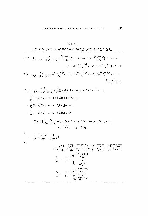
H(t,) = 0 (10) (again see Kwakernaak & Sivan, 1972). The system of equations (5)-(6) has been integrated in Appendix A. Table 1 displays the resulting curves V(t), i(t), P,(t) and P(t), for 0 5 t 5 t,, in terms of five integration constants ar-~1~. The boundary condition (9a) has been taken into account auto- matically, thus eliminating one integration constant. Now the logical sequence of calculations is the following. First consider the case where the ejection time t, is fixed. Then, for given values of the system parameters and the loading parameters V, and P,, k; is computed using equation (3), such that the boundary values (9b)-(9f) are known. Expressions for these boundary values, in terms of the integration constants ~,-a,, are obtained by evaluating the state variables x,(t), i = 1 . . 3, and the costate variable pj(l) at t = 0 and t = 2,. This is done using the formulas in Table 1. A formula for /am can easily be found using the results listed in Appendix A. This produces a

LEFT VENTRICULAR EJECTION I)YN.!hllC’S

TABLE 1

Optimal operation of the model during ejection (0 5 t 5 t,)

282 E. J. NOLDUS

system of linear algebraic equations in al-u5, which can be solved by computer in a straightforward manner. Substitution of the results in the expressions of Table 1 yields the desired solution.

If the ejection time t, is variable, then equation (10) is used to determine its optimal value. This must be done in a computer algorithm of successive approximations. N can be obtained by evaluating equation (7) at an arbitrary time. for example at t = 0 or at t = t,. For t = f, one ha<

If = L?(t,)+ ~(u-n,)-R~p, , L L,<.

where

u(t,) = - ;L P2(fJ,

such that equation (10) becomes

1 u2 - 2ux, +x-c pjx3 = 0, for t = t,. (11)

Now, for given values of the system and loading parameters, and for a fixed value of the weighting coefficient CI, the left hand side of equation (11) can be computed for any guessed value of t,. t, is adjusted by successive approximations until equation (11) holds. Then the calculations proceed as for the fixed final time problem. However, the relation (10) can also be used in a different way. Indeed, after selecting a normal value for t,, the corresponding value for CI can be obtained from equation (lo), thus conjecturing that the normal t, is optimal for the considered performance index. In this way an estimate is produced for the unknown weighting factor in the performance index. Again this is done in an algorithm of successive approximations, in which CI is adjusted until equation (11) holds, for a given t,. When doing so for normal values of all system parameters, a-values are obtained in the range of c( = 1 mm Hg/(ml/s) to c1 = 5 mm Hg/(ml/s).

The heart rate n, corresponding with a given set of parameter values can be obtained as follows: During the diastolic interval of duration t,, following the ejection period under consideration, and during a short isovolumic contraction of duration r, following diastole, the aortic valve is closed. Then the aortic pressure P,(t) decays exponentially with time constant RC. This can be verified in the circuit of Fig. I, where the capacitor C unloads over the resistor R while the valve is closed [i(t) E 01. In periodic operation, the aortic pressure at the end of isovolumic contraction, that is, at the end of the exponential decay, equals the aortic pressure at the starting point of ejection. This yields the relation

PO(O) = P,,(t,,) cup [ - (fd + r)/RC],

LEFT VENTRICULAR EJECTION DYNAMICS 283

or, t,+z = RC In [Pa(fJ/Po(0)]

from which the heart rate n = 60/(t,+~+t,)

can be computed.

4. General Results

Figure 2(a) curve A shows the time course of ventricular systolic pressure, for a set of parameter values for the human system, taken from Defares et ul. (1964). The origin of the time axis has been shifted to the starting point of the systolic phase, of duration t, = 0.2 s, which consists of the isovolumic contraction of duration z = 0.02 s and the ejection period of duration t, = 0.18 s. According to equation (10) the corresponding value for r) has been calculated to be a = 3.78 mm Hg/(ml/s). During the isovolumic contraction period, P(t) rises from its initial value, approximately zero, to the computed initial value for the ejection phase. Since z is a small fraction 01 the cardiac period, the pressure rise during this time interval can be approximated by a linear curve. The computed curve starts at the beginning of ejection. As a result, the systolic time course of P(t) exhibits two characteristic peaks, which have been observed in numerous experiments (Greene et al., 1973; Suga, 1969; Clark, Kane & Bourland, 1973). Although in representative data the primary peak is not always very pronounced, and may to some extent depend on the type of transducer used, the existence of two-peak pressure waves seems to be very consistent in experimental recordings. In Fig. 2(a) curve A the primary peak is very sharp as a result of the slope discontinuity at the beginning of ejection. This stems from the fact that the pressure curve has only been calculated during ejection, and hence a sharp primary peak is inherent to the computational procedure followed. The sharpness of the peak is of little importance however, the general form of the curve being mainly determined by the relative height of the first and the second peak, and the times at which they occur during systole. As will be shown in the following sections, the sharpness and relative heights of the peaks change with various system parameters and with loading conditions. For the nominal values of Fig. 2(a) curve A, the second peak occurs at I = 0,145 s, and both peaks have about the same height of 115 to 120 mm Hg. This corresponds approximately with data in Greene (1973). Suga (1969) and Buoncristiani, Liedtke, Strong & Urschel (1973). These papers report experimentally obtained pressure waves, also showing two peaks of approximately equal height, the first peak occurring at the beginning of ejection and the second one approximately at the beginning of the lasr

254

100

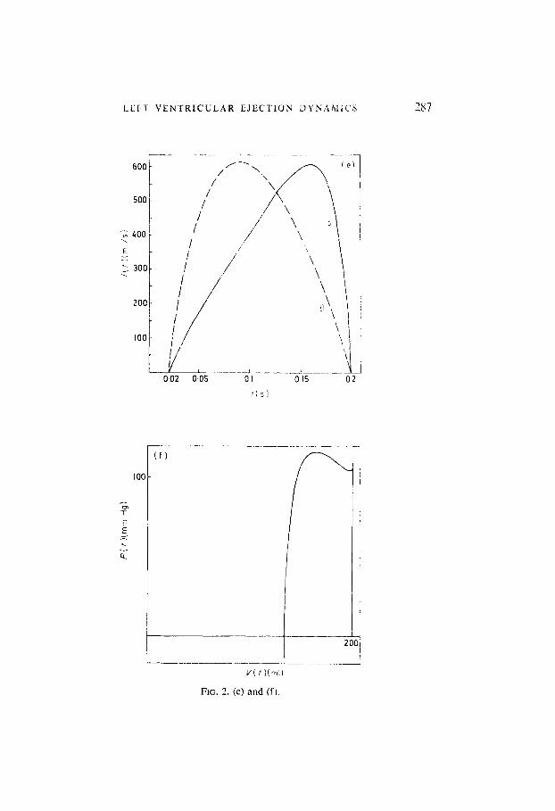
FIG. 2. (a) Curve A time course of ventricular systolic pressure, for the following co- efficients (a, c, d) in expression (3), and for the following parameter values (Defares et nl., 1964): a= -100 ml; d = OGO148 mm Hg-‘; c = 0.981; R .= 1 .O mm Hg/(ml/s): Y = 0.01 mm Hg/(ml/s); C = 1.9 ml!mm Hg; L = 0.003 mm Hg s2/mI; V0 = 200 ml; P,, = 100 mm Hg; r, = 0.18 s; r = 0.02 s; hence fs = 0.2 s; and tl = 3.78 mm Hg/(ml/s). Curve (B) experimentally recorded pressure wave, according to Greene et al. (1973), and Clark et al. (1973). normalized to the same maximum value and systolic period as curve (A). (b) ventricular systolic volume as a function of time; (c) systolic arterial pressure as a function of time; (d) curve (A) systolic elastance as a function of time. Curve (B) an experimentally determined elastance curve, according to Greene et al. (1973), normalized to the same maximum value and systolic period as curve (A); (e) Curve (A) blood flow as a function of time during ejection: Curve(B) blood flow as a function of time according to Defares ei al. (1964); (f) ventricular pressure-volume diagram.

150 -

5 = 100 - . x

50-

FIG. 2. (b) and (c).

286

r-

5-

.5 -

I

E. J. NOLDUS

-.-----~- .--

FIG. 2. (d).

LI:tT VENTRICULAR EJECTION DYNAMIC‘S ‘X7

600

/ 500

‘,G 400 -. I E x > 300 ‘.

200.

-1

100

FIG. 2. (e) and (f).

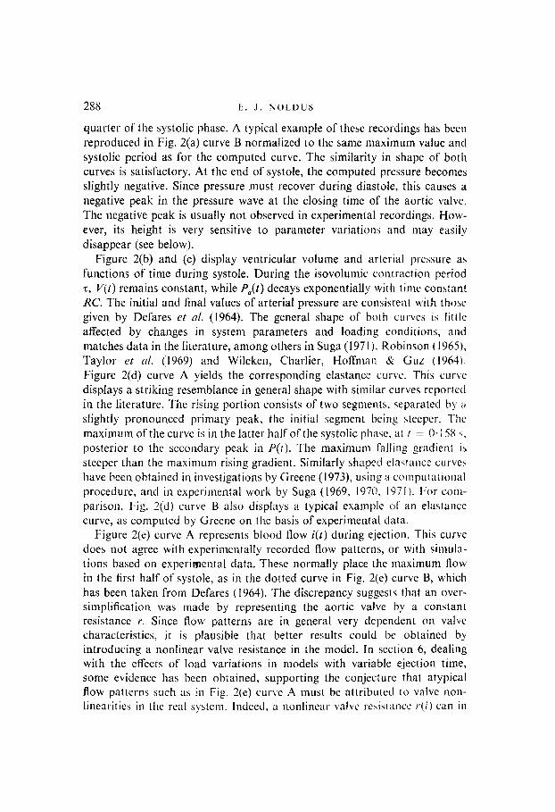
288 E. J. KOLDUS

quarter of the systolic phase. A typical example of these recordings has been reproduced in Fig. 2(a) curve B normalized to the same maximum value and systolic period as for the computed curve. The similarity in shape of both curves is satisfactory. At the end of systole, the computed pressure becomes slightly negative. Since pressure must recover during diastole, this causes a negative peak in the pressure wave at the closing time of the aortic valve. The negative peak is usually not observed in experimental recordings. Hou- ever, its height is very sensitive to parameter variations and may easily disappear (see below).

Figure 2(b) and (c) display ventricular volume and arterial pressure as functions of time during systole. During the isovolumic contraction period z, V(t) remains constant, while P,(t) decays exponentially with time constant XC. The initial and final values of arterial pressure are consistent with those given by Defares ct al. (1964). The general shape of both curves is little affected by changes in system parameters and loading conditions, and matches data in the literature, among others in Suga (197 I ), Robinson ( I96.5), Taylor et (11. (1969) and Wilcken, Charlier, Hoffman Rr Guz ( 1964). Figure 2(d) curve A yields the corresponding elastance curve. This curve displays a striking resemblance in general shape with similar curves reported in the literature. The rising portion consists of two segments. separated by a slightly pronounced primary peak, the initial segment being steeper. The maximum of the curve is in the latter half of the systolic phase. at f = 0. i 5X \. posterior to the secondary peak in P(r). The maximum falling gradient is steeper than the maximum rising gradient. Similarly shaped elnstancc curves have been obtained in investigations by Greene (1973), using :I compuln;ional procedure, and in experimental work by Suga (1969, 1970. 1971). For corn- parison, Fig. 2(d) curve B also displays a typical example ol‘ an elastancc curve, as computed by Greene on the basis of experimental data.

Figure 2(e) curve A represents blood flow i(t) during ejection. This curve does not agree with experimentally recorded flow patterns, or with simulations based on experimental data. These normally place the maximum flow in the first half of systole, as in the dotted curve in Fig. 2(e) curve B, which has been taken from Defares (1964). The discrepancy suggests that an oversimplification was made by representing the aortic valve by a constant resistance I’. Since flow patterns are in general very dependent on valve characteristics, it is plausible that better results could be obtained by introducing a nonlinear valve resistance in the model. In section 6, dealing with the effects of load variations in models with variable ejection time, some evidence has been obtained, supporting the conjecture that atypical flow patterns such as in Fig. 2(e) curve A must be attributed lo valve non- linearitics in the real system. Indeed, a nonlinear valve rehistancc /,(,i) can in

I.T:FT VENTRICULAR li.lFfTlC)N DYN4%:!< \

5 .

.3=5mm Hg/(ml/s)

7 \

1

/:

\I

'I

3

I

i

28?

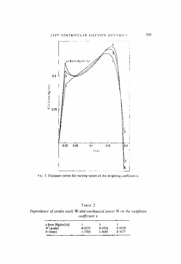
FIG. 3. Elastance curves for varying values of the weighting coefficient a.

TABLE 2

a [mm Hdb-d/s)l 1 3 5 W (joule) 0.9257 0.9228 0.9218 N (watt) 1.3705 1.3685 1.3677

290 E. J. NOLDUS

general be approximated by a constant value r if blood flow i(t) remains sufficiently small throughout ejection, the approximation becoming better for decreasing average and/or peak blood flow rates. In section 6, Fig. 1 I, flow patterns i(t) have been computed for varying end-diastolic volume V,. Since the flow curve generally decreases in amplitude for decreasing V,,, hence tending to eliminate the effects of possible valve nonlinearities, one would expect that for lower values of V,, the discrepancy between computed and actual flow curves should disappear. It can readily be observed that this ib in effect true. For decreasing V, the maximum in the flow curve shifts towards the middle of the ejection phase, and the flow pattern becomes symmetrical. completely in agreement with experimental curves (Suga, 1969, 1970), which also become symmetrical for low amplitude flow patterns.

The possibility of introducing a nonlinear valve model has not been further investigated, because of the computational difficulties involved in handling nonlinear systems, and because it is unclear exactly how valve resistance varies with blood flow. It should be noted that linear ejection models, in particular showing constant valve resistances during ejection, are widely used in the literature (Suga, 1971; Greene et al., 1973). Discrepancies in behaviour with the real system, resulting from nonlinearities in the real system, are a common characteristic of all these models.

A computed pressure-volume diagram is given in Fig. 2(f). Here the resemblance with experimental data (Greene, 1973; Robinson, 1965) ib satisfactory. As already noted, in Fig. 2(a)-(f) the weighting coefficient E was selected so, that the corresponding optimal ejection period t, takes a normal value, t, = 0.18 s. However, the sensitivity of waveforms to the precise value of M is small. Figure 3 presents elastance curves E(t) for varying values of ‘A and for a constant ejection time f,, all other parameters also remaining constant. For increasing c(, the maxima in the elastance curves become more pronounced, since less weight is attached to pressure peaks in the performance index. However, even relatively strong changes in u do not essentially alter the shape of the waveforms. As could be expected from the choice of the performance index, stroke work W and mechanical power IV transferred by the ventricle to the blood, decrease slightly for increasing 7, according to Table 2.

5. Effects of Load Variations

We shall start with investigating the effects of changing afterload conditions. First it must be observed that in the living system the mean arterial pressure P,, which constitutes the main afterload parameter, is not an independent variable. P, is affected by several factors, but is mainly controlled

I.EFT VENTRICULAR EJECTION DYNhMI(‘S 191

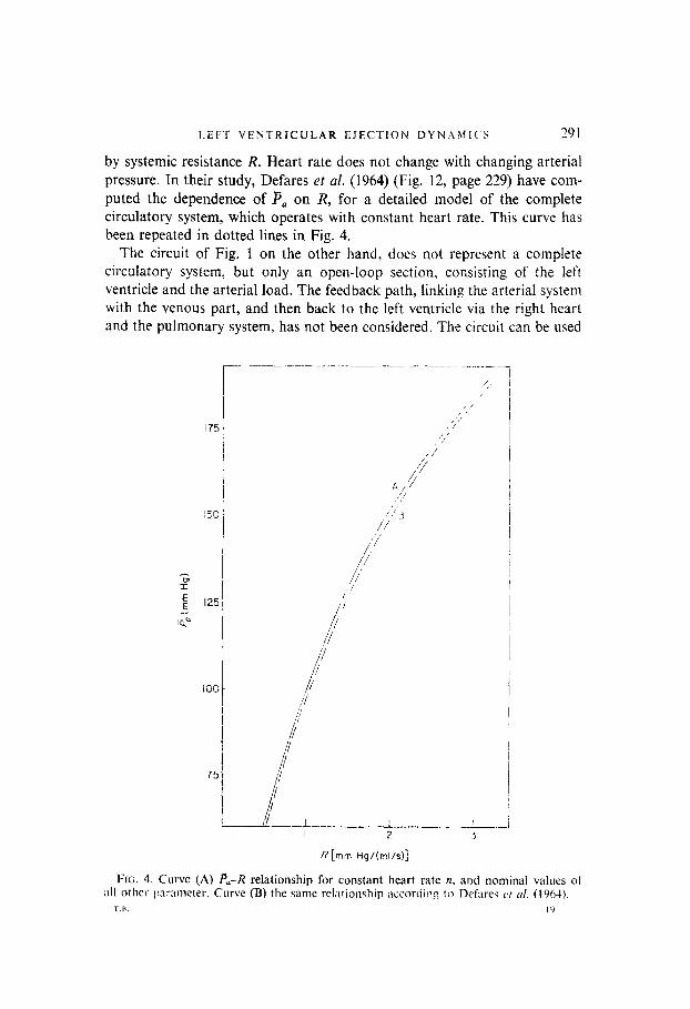
by systemic resistance R. Heart rate does not change with changing arterial pressure. In their study, Defares et al. (1964) (Fig. 12, page 229) have computed the dependence of P, on R, for a detailed model of the complete circulatory system, which operates with constant heart rate. This curve has been repeated in dotted lines in Fig. 4.

The circuit of Fig. 1 on the other hand, does not represent a complete circulatory system, but only an open-loop section, consisting of the left ventricle and the arterial load. The feedback path, linking the arterial system with the venous part, and then back to the left ventricle via the right heart and the pulmonary system, has not been considered. The circuit can be used

r ,

,;,’

/

‘/ /

R [mm Hg/(ml/si]

FIG. 4. Curve (A) pa-R relationship for constant heart rate n, and nominal values of all other pramcter. Curve (B) the same rel;ttionship accordin 2 to Defilres it 01. (1904).

T.ll. I ‘1

292 E. J. NOLDUS

to study the uncontrolled, open loop ejection system, in which P, and R can be changed independently. When doing so, increasing P, for constant systemic resistance R results in strongly growing heart rates, hence in drastic increases of transferred mechanical power N. More interesting results can be obtained by endowing the ejection model with an arterial pressure controller, which establishes a relationship between r’, and R, such as exists in the complete circulatory system. Since the pumping ventricle does not change its rate with changing arterial pressure, a good model for such a controller is the one which keeps heart rate ?I unaffected by changes in R and B,. The behaviour of the ejection model, controlled in this way, may then be compared with available experimental data, which mostly stem from measurements and simulations in which heart rate was kept constant.

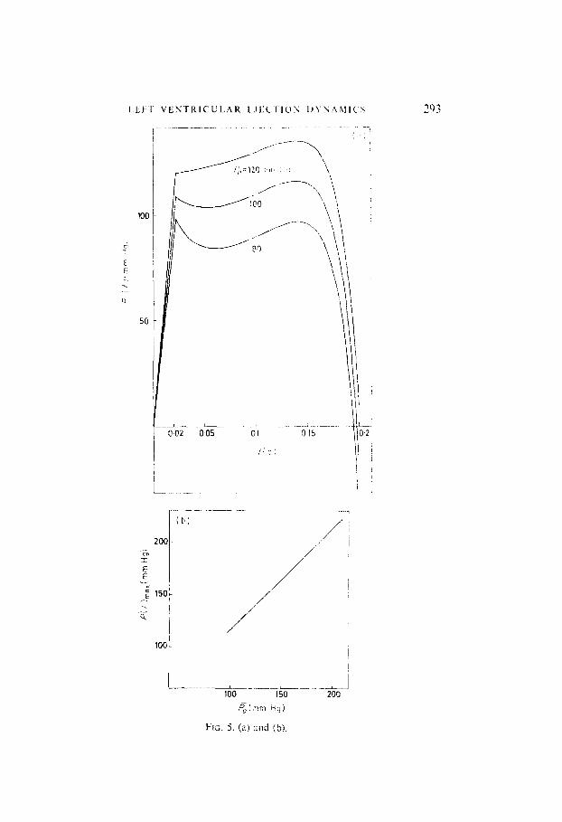
Figure 4 shows the computed relationship between P,, and R, for nominal values of all other parameters, such that 71 remains constant. This curve almost coincides with the Pa--R curve for constant II, obtained by Defares, although a more complicated loading network was introduced there, and a detailed model of the complete circulatory system was used. It follows that if our model is endowed with a PC,-R relationship, as exists in the complete closed-loop system, then heart rate is independent of mean arterial pressure, in agreement with the real system. In the present model, the nominal heart rate equals 12 = 89 min-‘. This is higher than normal, due to the simplification, introduced by selecting a linear, first-order arterial loading network. A better numerical value for II could be obtained at the expense of compli- cating loading dynamics, for example as suggested by Defares (1964), or by slightly adapting the peripheral resistance R. However, the exact value of heart rate scarcely affects systolic waveforms. Section 7 presents some results for a slightly increased resistance R, and normal heart rates. Plots of left ventricular pressure against time, for varying values of arterial afterload, and for a fixed ejection period t,, are shown in Fig. 5(a) [Figs 5-8 represent solutions of the fixed final time problem, with t,, = 0.1s s. which is optimal for the nominal parameter values, used in Fig. 2(a)]. The left ventricular pressure waveform generally increases in amplitude with increasing I-‘,,, conform with results in Greene (1973). Suga (1971), Taylor (1969). Buoncristiani (1973), Wit&en (1964). The secondary peak in the wavelbrm increases steadily as a function of increasing load, until it becomes dominant over the primary peak. For high values of P,, P(r) exhibits a single maximum in the latter half of the systolic phase. This increase in the secondary peak with increasing afterload is frequently observed experimentally, and also appears in calculated curves by Greene (1973). Increasing 7, also increases end- systolic pressure, which becomes positive for B, = 120 mm Hg. The secondary peak time remains almost constant, as confirmed by Greene.

L

I

-.---I_- ---_L---_. -----L. 100 150 200

P,t,nrn Hg)

FIG. 5. (a, 2nd (b).

294 E. J. NOLDUS

,j.6 ’ t

05 j-

I.----_~ I 1-J 100 150 200

&!mm Hg)

---- J. - -- - --L_~- .-. -_1--

100 150 200

,Po (mm fig)

FIG. 5. (a) Ventricular pressure curves for varying afterload conditions (ejection period t, and heart rate IZ constant); (b) maximum ventricular pressure P(f),,,,, as a function of mean arterial pressure Pa: (c) stroke work W as a function of Pa; (d) mechanical power N as a function of Pa, for constant heart rate and for varying heart rate.

Maximum pressure P(t),,,, as a function of P, is shown in Fig. 5(b). This again corresponds with Greene’s curve, which is also essentially linear. In Fig. 5(c) and (d), stroke work Wand transferred mechanical power N have been computed as functions of P,. Figure 5(c) is the typical parabolic curve which can also be found in Sonnenblick & Downing (1963) and in Suga (1971). Stroke work and mechanical power are maximum at is, = 160 mm Hg. Figure 5(d) also shows transferred mechanical power in the case where systemic resistance is kept constant, hence the heart rate II is allowed to vary.

LEFT VENTRICULAR EJECTlON DYNAMICS

(b) 140 .-

2

E -i

F 130-

I-I_--____L_-- 160 186 200 220

PO (I?!

FE. 6. (a) and (0).

295

296

I 1 ---L-L- 160 180 200 220

V. (ml)

I.7

------. I--~---.L .-~~~ 180 200 220

V,(rnll

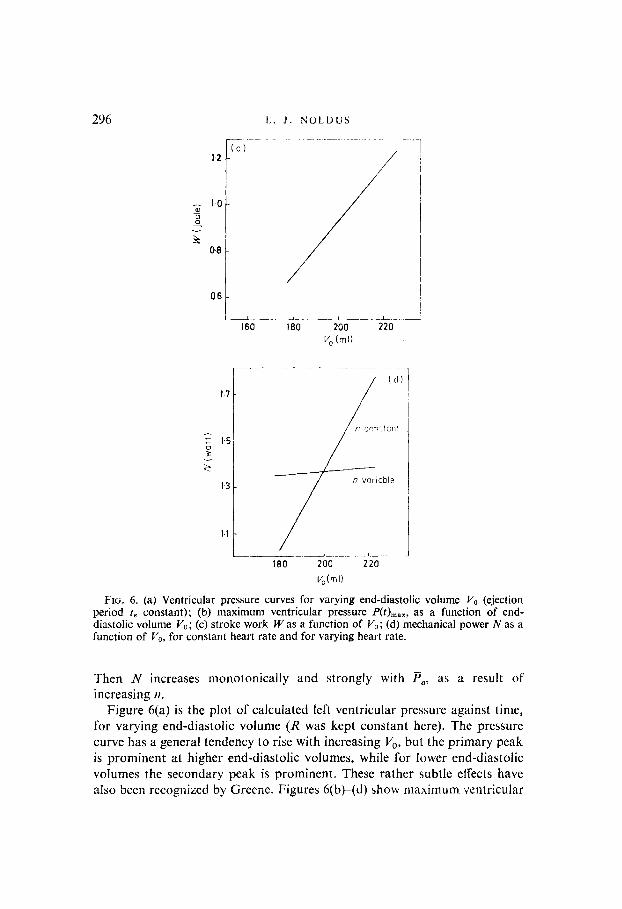
FIG. 6. (a) Ventricular pressure curves for varying end-diastolic volume VO (ejection period t, constant); (b) maximum ventricular pressure P(r),,,, as a function of end- diastolic volume V,,; (c) stroke work Was a function of VO; (d) mechanical power N as a function of V,, for constant heart rate and for varying heart rate.

Then N increases monotonically and strongly with P,, as a result of increasing II.

Figure 6(a) is the plot of calculated left ventricular pressure against time, for varying end-diastolic volume (R was kept constant here). The pressure curve has a general tendency to rise with increasing V,, but the primary peak is prominent at higher end-diastolic volumes, while for lower end-diastolic volumes the secondary peak is prominent. These rather subtle effects have also been recognized by Greene. Figures b(b)-(d) show maximum ventricular

LEFT VENTRICULAR EJECT’ION DYNAMICS ‘97

pressure P(r),,,, stroke work W and mechanical power N, as functions of V,. The slope discontinuity in the first curve stems from the fact that, at lower values of V,, the maximum pressure coincides with the secondary peak, while at higher V,, the maximum coincides with the primary peak. This curve does not agree with Greene’s recordings, which display a maximum for some intermediate V,,. The plots of W and N against V,, are linear, and do not reach an extremum within the normal range of the end-diastolic volume (cf. Suga, 197 1; Robinson, 1965). Figure 6(d) also shows mechanical power N versus P’,,. in the case where n is kept constant, by varying V, and R simultaneously. Now N increases strongly with iJO, as a result of increasing stroke volume VS.

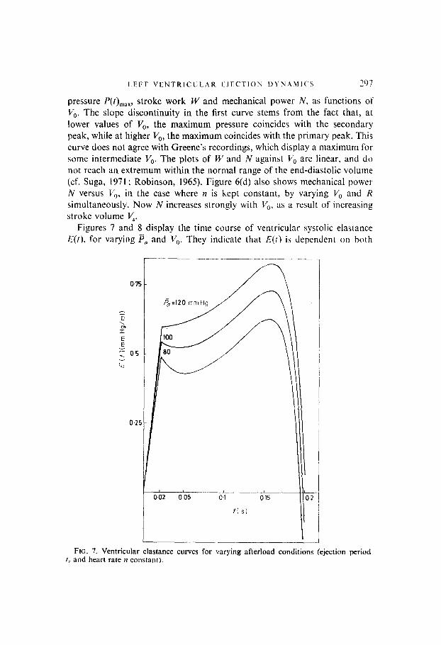
Figures 7 and 8 display the time course of ventricular systolic elastance E(t), for varying P, and V,. They indicate that E(r) is dependent on both

0,7!

E \ I”

E F 05

G

O-2’

Fro. 7. Ventricular elastance curves for varying afterload conditions (ejection period I, and heart rate II constant).

298

I I I --

0-02 0.05 01 045

i(s)

FIG. 8. Ventricular elastance curves for varying end-diastolic volume (ejection period t, constant).

preload and afterload conditions. Specifically, the E(t)-waveforms increase in amplitude for increasing H,, and decrease for increasing V,,. The latter result confirms experimental findings in the paper by Greene, but contradicts Suga (1969), according to whom elastance curves are essentially independent of loading conditions. Variations in the time course of v(t), i(t) and P,(t) with is, and V,, are conformable to data in the literature, and have not been reproduced here.

6. Cases with Variable Ejection Time

In this section some results are presented, pertaining to the free final time problem. For a fixed value of the weighting coefficient ~1, the ejection time f, is optimized using the condition (10). Figure 9 shows two pressure curves for

- -.(I

-

002

005

01

t(s)

01

Hg

Fw.

9.

Vent

ricul

ar

pres

sure

cu

rves

fo

r no

min

al

and

decr

ease

d m

ean

arte

rial

pres

sure

Pa

,, an

d fo

r a

varia

ble

ejec

tion

perio

d [x

:

2.5

mm

H

gKm

l,‘s)

].

0’02

-I-.

..-~

0.05

FIG

. 10

. Ve

ntric

ular

pr

essu

re

curv

es

for

nom

inal

an

d in

crea

sed

end-

dias

tolic

vo

lum

e V,

, an

d fo

r a

varia

ble

ejec

tion

perio

d [a

7

2.5

mm

Hg,

Yml/s

)].

300 I:. J. NOLDIJS

a = 2.5 mm Hg/(ml/s), and for the nominal and a decreased value of mean arterial pressure. Analogous results for the nominal and an increased value of V, are given in Fig. 10. Comparing with Fig. 2(a) reveals that t, decreases with decreasing a (10% change in t, for more than 25% change in a), and that t, increases for decreasing P, and for increasing V,. The latter properties are well known from numerous results in the literature (Greene, 1973; Suga, 1969; Buoncristiani, 1973; Wilcken, 1964), although the present recordings suggest a stronger dependence of ejection time on loading conditions, than is usually observed experimentally. Figure 11 shows flow patterns i(t) for varying V,. As already pointed out, the flow curve becomes symmetrical for lower values of V,, in accordance with experimental data (Suga, 1969).

600-

FIG. 1 I. Blood flow curves for varying end-diastolic volume, and for a variable ejection period [LY : 1.5 mm Hg/(ml/s)].

LEFT VENTRICULAR EJECTION DYNAhlIC‘S 301

7. Effects of Other Parameters

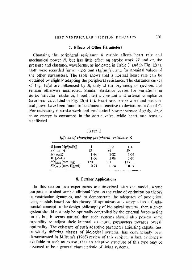
Changing the peripheral resistance R mainly affects heart rate and mechanical power N, but has little effect on stroke work W and on the pressure and elastance waveforms, as indicated in Table 3, and in Fig. 12(a). Both were recorded for c( = 2.5 mm Hg/(ml/s), and for nominal values of the other parameters. The table shows that a normal heart rate can bc obtained by slightly adapting the peripheral resistance. The elastance curves of Fig. 12(a) are influenced by R, only at the beginning of ejection, bul remain otherwise unaffected. Similar elastance curves for variations in aortic valvular resistance, blood inertia constant and arterial compliance have been calculated in Fig. 12(b)-(d). Heart rate, stroke work and mechanical power have been found to be almost insensitive to deviations in L and c’. For increasing r, stroke work and mechanical power increase slightly, since more energy is consumed in the aortic valve, while heart rate remains unaffected.

TABLE 3

Effects of changing peripheral resistance R

R [mm WW/sN 1 1.2 1.4 n (min-I) 83 69 59 N (watt) 1.46 1.22 1.04 W (joule) 1.06 1.06 1.06

J’@hn,x (- Hg) 120 121 123 Wh, (mm Hg/ml) 0.74 0.74 0.74

8. Further Applications

In this section two experiments are described with the model, whose purpose is to shed some additional light on the value of optimization theory in ventricular dynamics, and to demonstrate the adequacy of prediction, using models based on this theory. If optimization is accepted as a fundamental concept in the design philosophy of biological systems, then a given system should not only be optimally controlled by the external forces acting on it, but it seems natural that such systems should also possess some capability to adjust their internal structural parameters towards overall optimality. The existence of such adaptive parameter adjusting capabilities, in widely differing classes of biological systems, has convincingly been demonstrated in Milsum’s (1968) review of this subject. In fact, evidence is available to such an extent, that an adaptive structure of this type may bc assumed to be a general characteristic OF living systems.

L I I 1 O

.! -

__-_-

-l_

r-- (b)

OM

5 1

c I I__

_--.

002

005

01

0.15

t(s)

0 01

5 m

m

Hg/!m

i/s

J

FIG

. 12

. (a)

Ela

stan

ce

curv

es f

or v

aryi

ng

perip

hera

l re

sista

nce

R [a

:-=

2.5

mm

Hg;

(ml/s

)J;

(b)

elas

tanc

e cu

rves

for

var

ying

ao

rtic

valv

ula

resis

tanc

e r;

(c)

elas

tanc

e cu

rves

fo

r va

ryin

g bl

ood

iner

tia

cons

tant

L:

(d

) el

asta

nce

curv

es f

or v

aryi

ng

arte

rial

com

plia

nce

C.

304 L. J. NULDUS

In Fig. 13, it has been assumed that in the blood ejection mechanism, entl- diastolic volume l’,, can be adaptively adjusted on the basis of minimizing energy consumption. Figure 13 shows the mechanical work N,., generated by the ventricle per unit of ejected blood volume, represented in normalized form (relative to its minimum value), against I/,,. The plot reveals that the

V. (ml)

FIG. 13. Mechanical work per unit of ejected blood volume (in normalized form, relative to its minimum vaIue), as a function of V,, for nominal values of all other parameters.

best value for V0 approximately equals the nominal value of 200 ml. It certainly adds to the consistency of the system’s behaviour, and to the value of the optimization concept, if in a model that was optimally designed on energetic considerations, the nominal value of a loading parameter is also energetically the best one.

The second example describes a case of ventricular ejection under abnormal operating conditions. The model has been used to simulate aortic stenosis, which consists of an obstruction of blood flow from the ventricle to the

--- 0.02 0.05 01 015

f(s)

1 0

FIG. 14. Curve (A) computed ventricular pressure wave in the case of simulated aortic stenosis; curve (B) computed normal ventricular pressure wave; curve (C) experimentally recorded ventricular pressure wave in a case of aortic stenosis, according to Van der Werf (1974). normalized to the same maximum val:ie and systolic period as curve (A).

306 E. J. NOLDUS

aorta, and is usually caused by a striction near the aortic valve. Aortic pressure is usually below normal. Heart rate remains normal or decreases slightly, while the systolic period increases. Recorded ventricular pressure curves for this condition can be found in Van der Werf (1974). They are characterized by a strongly increased secondary peak. In order to simulate aortic stenosis, the following parameter values were introduced in the model : Aortic resistance Y was increased to 0.05 mm Hg/(ml/s), mean arterial pressure was set at 75 mm Hg, and, according to Fig. 4, systemic resistance at O-7 mm Hg/(ml/s). The systolic interval was increased to 0.22 s. Figure 14 shows the resulting pressure wave, as compared to the normal one, and also an experimental curve according to Van der Werf (1974). The increased secondary peak is correctly reproduced, which shows that the model is not only capable of predicting the ventricle’s behaviour under normal operating conditions, but also in abnormal situations.

In addition the simulation provides some evidence that the ventricle’s optimal control mechanism does not operate on a preprogrammed, or “open loop” basis, either genetically or learned, but upon a basis of continuing adaptive control. By this is meant that the control strategy can be con- tinuously and optimally modified upon the occurrence of structural changes in the controlled system, for example as a result of illness. It is evident that such adaptive aspects essentially enhance the power and quality of biological control.

9. Discussion

A model of the left ventricular ejection system has been developed, which has as its salient feature the optimization of the ventricular elastance curve E(l) with respect to a performance index, selected on an energetic basis. The ventricle has been loaded with a lumped arterial Windkessel load. Although the performance index is very simple, the model is capable of correctly reproducing many classical experimental results, at least in a qualitative sense, including the changes in left ventricular pressure curves in response to varying preload and afterload conditions (changes in end-diastolic volume V, and mean arterial pressure P,). The model accurately predicts the shape of the left ventricular pressure wave, as well as subtle modifications in this shape, as a function of increasing arterial pressure and end-diastolic volume. Computing the corresponding ventricular elastance yields a family of elastance curves, depending on P, and V,. The dependence is qualitatively in agreement with the results of Greene et al. (1973). It is in contrast however with those of Suga (1969, 1971), according to whom ventricular elastance is essentially independent of P, and I’,. When the ejection period is allowed to

LEFT VENTRICULAR EJECTION DYNAMICS 3.);

change, it decreases for decreasing k;, and for increasing I’,, also in agreement with experimental findings. The model is not capable of satisfactorily reproducing the time course of blood flow during ejection. Possibly this can be attributed to an oversimplification in simulating aortic valve characteristics by a constant resistance. Some evidence supporting this conjecture has been included in the paper. For reduced end-diastolic solumes and the corresponding lower amplitude flow patterns, the discrepancy between computed and experimental flow curves tends to disappear, probably as ;I result of the reduced influence of valve nonlinearities. Finally the effects of changing peripheral resistance, blood inertia constant and arterial compliance have been briefly examined, and the model’s operation in an :tbnormal condition of the controlled system has been discussed. It has been thown that the real system’s behaviour is, in a qualitative sense. adequately predicted under abnormal as well as normal condi:ions of the controlled system. In addition an example has been provided in which the nominal value of a loading parameter is successfully matched with the energetically optimal value for this parameter, thus further supporting the optimization concept as a fundamental principle in the design of the ejection mechanism.

Complete numerical agreement with experimental data has not alway\ been achieved. This could not be expected however. in view of the simplified qualitative nature of the dynamical model. upon which the analysis wa\ carried out. Nevertheless the results strongly suggest that the general control strategy, including shapes of waveforms and their dependence on system parameters, and the nominal values of these parameters, are probably related to energy minimization considerations. Further research might be directed towards the analysis of more accurate dynamical ejection models on a similar basis, possibly including the entire cardiovascular system, ancl taking into account a number of homeostatic relationships among parameters. which in the present analysis have been ignored or crudely approximated. Using a more realistic arterial loading network might also be attempted. Of course this could only be done at the expense of strongly increased computational complexity.

The author is grateful to H. Hinssen and E. Van Tngelghem who wrote the computer program for the present problem.

APPENDIX A

Integration of the Hamiltonian System, equations (5)--(b)

First note that p1 = a,, a constant. Define z, A y2 + aLx,, zz 4 p2 -ah,. --.I 4 (PJC) +a.~,, and - L4 4 (p,/C)--KY,. Then. by iwice differentiating z, and

r 9. 31

308 E. J. NOLDUS

rearranging terms, it is easy to show that

Eliminating z2 from equations (Ala)-(Alb) yields a fourth order equation in zI, from which 21 = P(r) = -z,/2L can be obtained as given in Table I, in terms of the integration constants a,-a5. Now the computation of

-6,La,] e -6z(fe-‘)+[(C(+J.)UJ+S*L~4] e-d?r

-f-[(~+~.)f~~+K,Li(~] e-“1’

and the results of Table 1 is straightforward.

REFERENCES BENEKEN, J. E. W. (1964). In Palsatile Blood Flol!j (E. 0. Attinger, ed.), pp. 423-432.

New York: McGraw-Hill. BUONCKISTIANI. J. F., LIEDTKE, A., STRONG. R. & URSCHEI, C. (1973). IEEE Trans. Biomctl.

Eng. 20, 110. CLARK, J. W., KANE, G. & BOURLAND, H. (1973). IEEE Trans. Biamed. Eng, 20, 404. DEFARES, J. G., HARA, H., OSBORN, J. & MCLEOD, J. (1963). In Circulato,:,~ Aaa/a,~

Cor~lprrtevs (A. Noordergraaf, ed.), pp. 91-121. Amsterdam : North-Holland Publ. Co. DEFARES, J. G., OSBORN, J. & HARA, H. (1964). Acta Physiol. Pharmarol. Neerrl. 12, 189. GREENE, M. E., CLARK, J., MOHR, D. & BOURLAND, H. (1973). Med. Biol. Eng. 11, 1%. KWAKERNAAK, H. & SWAN, R. (1972). Linear Optimal Control Systems. New York: Wiley. MILSUM, J. H. (1968). In Advances in Biomedicdl Engineering ond Medic& Phj:sics (S. N.

Levine, ed.), vol. I, pp. 243-278. New York: Interscience Publ. NOORDERGRAAF, A. (1969). In Biological Engineering (H. P. Schw;ln, ed.), pp. 391-545.

New York: McGraw-Hill. ROBINSON, D. A. (1965). Circ. Res. XVII, 207. SONNENBLICK, E. H. & DOWNING, S. E. (1963). Am. J. Plr,~sioZ. 204. 604.

LEFT VENTRICULAR I-JECTION IlYhh.MICS 309

SLIC;~, H. (1069). Jdp. Hedrt J. 10, 509. SUGA, H. (1970). Jdp. Heart J. 11, 373. SUGA, H. (1971). IEEE Truns. Biomed. Eng. 18, 47. TAYLOR, R. R., COVELL, J. & Ross, J. (1969). AM. J. Ph~siol. 216, 1097. VAN DER WERF, T. (1974). Klinische Puiholysiologie wz /ret Hurf. Utrecht: Oosthod WARNER, H. R. (1965). In Hdndbook oy PlrjGh~jl (W. F. Hamilton 6: P. Dw, &I.

sect. 2, vol. 3, pp. 1825-1841. Washington, D.C.: Am. Physiol. Sot. WILCKEN, D. E.. CHARLIER. A., HOFFMAN, J. & Cuz, A. (1904). Ci~~~~d. /Gs. XIV. X.3.

optimal control aspects of left ventricular ejection dynamicsoda/contents/01matem%e1tic… · ·...

Documents