optimal detection in the k-distributed clutter … · for such a radar target, coherent detection...
TRANSCRIPT

UNCLASSIFIED
Optimal Detection in the K-Distributed Clutter Environment -- Non-Coherent Radar Processing
Yunhan Dong
Electronic Warfare and Radar Division Defence Science and Technology Organisation
DSTO-TR-2785
ABSTRACT Non-coherent detection of Gaussian targets (Swerling II targets) in the K-distributed clutter environment is investigated. The optimal detector is derived based on the Neyman-Pearson principle. It is shown to be the well-known square-law detector. Amplitude detector, log detector, and the like are not optimal, and result in some detection loss. Temporally correlated clutter provides a target gain, and improves detection. The higher the temporal correlation, the higher the target gain. Spatially correlated non-Gaussian clutter can also provide a CFAR gain. The autoregressive technique is used to optimally estimate the texture of the clutter. That in turn significanly improves the detection compared to the traditional cell-averaging processing.
RELEASE LIMITATION
Approved for public release
UNCLASSIFIED

UNCLASSIFIED
Published by Electronic Warfare and Radar Division DSTO Defence Science and Technology Organisation PO Box 1500 Edinburgh South Australia 5111 Australia Telephone: (08) 7389 5555 Fax: (08) 7389 6567 © Commonwealth of Australia 2012 AR-015-478 December 2012 APPROVED FOR PUBLIC RELEASE
UNCLASSIFIED

UNCLASSIFIED
Optimal Detection in the K-Distributed Clutter Environment -- Non-Coherent Radar Processing
Executive Summary In the maritime environment, radar detection unavoidably needs to deal with undesired signals, primarily sea clutter (echoes from the sea surface). How to detect target signals, especially relatively weak ones, against the clutter is challenging. Optimal detectors, based on the Neyman-Pearson principle, that maximise the probability of detection for a given false-alarm rate are the most interesting detectors to the radar community. Their derivation depends on the statistical models of both the clutter and the target. In a recent paper, ‘Optimal coherent radar detection in a K-distributed environment’ we have discussed the problem of optimal coherent detection. This report focuses on the non-coherent detection of Gaussian targets (Swerling II targets) in the compound K-distributed clutter environment. This report makes the following three contributions. First the optimal detector for multi-look non-coherent detection of Gaussian targets in the compound K-distributed clutter is derived. The optimal detector derived is shown to be the well-known square-law detector. This is because the clutter undergoes a Gaussian random process during the multi-look processing period (i.e., the multi-pulse processing period), as the slowly-varying component of the compound clutter remains unchanged during the period, according to the assumption. Although the derived optimal detector is not new, the derivation itself has a guiding meaning. As the detector has been rigorously derived for the first time using the Neyman-Pearson principle, it means that no other detectors exist which would perform better for the given conditions. Other detectors, such as the multi-look amplitude detector, the multi-look log detector, and the like are not optimal and inherently result in some detection loss. Secondly we have shown that for temporally correlated clutter, the use of a multi-look whitening process provides a target gain and improves the detection. The higher the correlation, the larger the target gain. The target gain comes from the difference between the spectrum of the correlated clutter and the spectrum of uncorrelated target signals (a non-uniform spectrum against a uniform spectrum), providing a second characteristic (in addition to the intensity) for discriminating the target from the clutter. On the other hand, if both the clutter and the target signals are individually uncorrelated (the cross-correlation between the two is always zero), each of them has a
UNCLASSIFIED

UNCLASSIFIED
UNCLASSIFIED
uniform spectrum, and there is only one characteristic (intensity) that can be employed in the detection. Therefore the event of the uncorrelated Gaussian targets embedded in the uncorrelated compound clutter represents the worst scenario in terms of detection. If the correlation of the target signals is the same as the correlation of the clutter, a treatment of de-correlation leads to the same processing for the uncorrelated target in the uncorrelated clutter. Lastly, spatially correlated non-Gaussian clutter may be able to provide some constant false-alarm rate (CFAR) gains. The CFAR gain is dependent on the estimate of the local mean. For this analysis we have examined the use of the linear autoregressive technique and derived the optimal weights for estimating the local mean of clutter. The autoregressive estimation is optimal under the linear assumption and better than the traditional cell-averaging estimation. The optimal estimation (under the linear assumption) of the clutter texture has in turn resulted in a further significant detection improvement (a few dB) for highly spatially correlated K-distributed clutter compared to the traditional cell-averaging estimation. This work was carried out in support of the ADF’s Air 7000 Project. Reference
Dong, Y. (2012), "Optimal coherent radar detection in a K-distributed clutter
environment", IET Radar, Sonar and Navig., 6(5), 283-292.

UNCLASSIFIED
UNCLASSIFIED
Author
Yunhan Dong Electronic Warfare and Radar Division Dr Yunhan Dong received his Bachelor and Master degrees in 1980s in China and PhD in 1995 at UNSW, Australia, all in electrical engineering. He then worked at UNSW from 1995 to 2000, and Optus Telecommunications Inc from 2000 to 2002. He joined DSTO as a Senior Research Scientist in 2002. His research interests are primarily in radar signal and image processing and clutter analysis. Dr Dong was a recipient of both the Postdoctoral Research Fellowships and Research Fellowships from the Australian Research Council.
____________________ ________________________________________________

UNCLASSIFIED
UNCLASSIFIED
This page is intentionally blank

UNCLASSIFIED DSTO-TR-2785
Contents
ACRONYMS ............................................................................................................................III
1. INTRODUCTION............................................................................................................... 1
2. JUSTIFICATION OF K-DISTRIBUTED CLUTTER .................................................... 2
3. OPTIMAL DETECTOR FOR NON-COHERENT DETECTION ............................... 3 3.1 Uncorrelated Clutter................................................................................................. 3 3.2 Clutter with Temporal Correlation...................................................................... 12
3.2.1 Case I: ................................................................................... 13 sf MM
3.2.2 Case II: .................................................................................. 14 sf MM
4. DETECTION AGAINST SPATIALLY CORRELATED CLUTTER ........................ 19 4.1 Estimation of Local Texture .................................................................................. 20 4.2 Results....................................................................................................................... 23
5. SUMMARY ........................................................................................................................ 28
APPENDIX A: SUMMATION OF NON-COHERENT DETECTION PROCESS ... 31
APPENDIX B: APPROXIMATION OF GAUSSIAN SIGNAL ADDED IN K-DISTRIBUTED CLUTTER ..................................................................... 35
APPENDIX C: TEMPORAL AND SPATIAL CORRELATIONS OF COMPOUND K-DISTRIBUTED CLUTTER ...................................... 43 C.1. Temporal Correlation (Correlation in Azimuth)...................... 43 C.2. Spatial Correlation (Correlation in Range) ............................... 44
APPENDIX D: INVERSE OF COVARIANCE MATRIX.............................................. 47
APPENDIX E: DISTRIBUTION OF MULI-LOOK CORRELATED K-DISTRIBUTED DATA ............................................................................ 49
UNCLASSIFIED i

UNCLASSIFIED DSTO-TR-2785
This page is intentionally blank
UNCLASSIFIED ii

UNCLASSIFIED DSTO-TR-2785
Acronyms
AR autoregressive CA cell averaging CAGO cell averaging greatest of CFAR constant false-alarm rate CUT cell under test GLRT generalised likelihood ratio test LMAP maximum posteriori estimation in the logarithm domain LRT likelihood ratio test MLE maximised likelihood estimate N-P Neyman-Pearson OS ordering statistic ROC receiver operating characteristic SCR signal-to-clutter ratio
UNCLASSIFIED iii

UNCLASSIFIED DSTO-TR-2785
UNCLASSIFIED iv
This page is intentionally blank

UNCLASSIFIED DSTO-TR-2785
1. Introduction
In a journal paper, ‘Optimal coherent radar detection in a K-distributed clutter environment’ (Dong 2012), we have proposed an optimal detector for coherent detection against K-distributed clutter. This report develops optimal and near optimal detectors for non-coherent detection. In the past, radar systems had relatively low resolution capabilities, and the Gaussian clutter assumption was a valid model for the clutter. With the advances in radar technology, the resolution capabilities of radar have been greatly improved in recent years. Clutter collected using high resolution radar systems exhibits non-Gaussian behaviour. The associated problem of optimal detection in a non-Gaussian background remains to be solved. The compound K-distribution, for instance, is a non-Gaussian distribution commonly used to model radar sea clutter; one of the milestone findings in radar clutter analysis and research in resent years (Ward et al. 2006). Researchers have been studying the optimal coherent detection of radar targets embedded in compound-Gaussian clutter for many years (Sangston et al. 2010; Sangston and Gerlach 1994; Sangston et al. 1999; Gini et al. 1999; Farina et al. 1997; Gini et al. 1998). While the matched filter is optimal for Gaussian clutter, the paper (Dong 2012) shows that the proposed optimal detector for K-distributed clutter significantly improves the detection compared to the matched-filter if clutter is highly spiky (i.e., K-distributed clutter with a small shape parameter). Therefore, there seems a need to investigate the optimal non-coherent detection against the K-distributed clutter. Non-coherent detection against K-distributed clutter has received equal attention. Armstrong and Griffiths (1991) studied detection of fluctuating targets in spatially correlated clutter, but their study focused on the performances of cell-averaging (CA), cell averaging greatest of (CAGO), and ordering statistic (OS) constant false-alarm rate (CFAR) processors and did not discuss the issue of optimal detection. Watts, Ward and Tough studied CFAR loss and CFAR gains associated with the K-distributed clutter (Watts 1996; Watts et al. 2007; Watts 1987). It has been found that for the compound Gaussian clutter, such as K-distributed clutter, CA-CFAR can provide a CFAR gain, provided that the texture of clutter (underlying mean) is correlated (Watts 1985). The higher the correlation, the larger the CFAR gain. Watts (1985) thus proposed a concept of ‘ideal CFAR’ which means that if the exact mean of the clutter for the cell under test (CUT) is known or estimated by other means, the best performance can be achieved. Based on this concept, Buccuarelli et al (Bucciarelli et al. 1996) proposed to use the maximum a posteriori estimation in the logarithm domain (LMAP) to estimate the local mean for the CUT. They found that the performance of LMAP-CFAR outperforms CA-CFAR especially when the correlation of the texture is high. A pulsed Doppler radar, equipped with a single transmitter and a single receiver, usually collects two-dimensional data, one dimension is time (separated by pulses) and the other is range (separated by range bins). This kind of data is often referred to as multi-look data. The associated detection problem is how to process this two-dimensional data to achieve
UNCLASSIFIED 1

UNCLASSIFIED DSTO-TR-2785
the detection goal. Apparently the above studies of non-coherent detection only consider the processing in the range domain. Conte et al (1999) proposed a generalised likelihood ratio test (GLRT) model for the optimal incoherent detection of Swerling II targets in the compound K-distributed clutter. However the model assumes that for the hypothesis only the first portion of an incoherent pulse train contains the clutter and target signal, and the second portion the pulse train contains clutter only. This condition does not seem to be robust to an unknown target location.
1H
In this report we first consider the processing in the time domain. Different assumptions for target signal and clutter lead to different designs of detection scheme in order to achieve the optimal and near-optimal performance. This report considers Swerling II model as the target model, i.e., target RCS is independent from pulse to pulse and varies with Gaussian. For such a radar target, coherent detection is not appropriate, because target signal’s phase varies randomly, and both target signals and clutter have a uniform spectrum in the frequency domain. Often we need to detect the intensity of the target signals. The intensity is enhanced by multiple look non-coherent integration. For Gaussian clutter, the multi-look intensity averaging processing is optimal. However whether it is still optimal for non-Gaussian clutter is remains to be answered. This report tries to derive optimal and/or near optimal detector from the Neyman-Pearson principle (Kay 1998, page 174). The unwanted signals that need to be considered in the maritime environment include echoes from the sea surface plus thermal noise of the radar receiver. In this report, the unwanted signals are assumed to be represented by a compound K-distribution (this is justified in Section 2). We derive optimal and near-optimal detectors based on the Neyman-Pearson principle in Section 3. The performance of optimal and near optimal detectors for temporally correlated clutter is also analysed. Secondly we study the processing in the range domain. Specifically we consider in Section 4 the non-coherent detection for the spatially correlated clutter. We use the autoregressive (AR) technique to optimally estimate the texture of clutter. That in turn significantly improves the detection compared to the traditional CA processing.
2. Justification of K-distributed Clutter
In a maritime radar surveillance environment, sea clutter has been verified, through numerous trials, to fit with the compound K-distribution for most conditions (Ward et al. 2006; Crisp et al. 2006; Dong and Merrett 2010; Greco and Gini 2007; Farina et al. 1997). Horizontally polarised higher resolution sea clutter may even have a heavier tail in its probability density function (pdf) and fits better with other distributions, such as KA (Watts et al. 2005), KK (Dong and Haywood 2007) and Pareto (Farshchian and Posner 2010) distributions. This report assumes sea clutter to be K-distributed. The compound K-distribution is composed of two components, a fast-varying component, referring to
UNCLASSIFIED 2

UNCLASSIFIED DSTO-TR-2785
speckle and a slowly-varying component, referring to the underlying mean or texture. The fast-varying component is a zero mean, unit variance complex Gaussian process modulated by the slowly-varying component, whose intensity is gamma distributed (Ward et al. 2006). Thermal noise, according to its nature, is often modelled by a Gaussian random process. The distribution of the sum of the K-distributed clutter and Gaussian thermal noise unfortunately does not have closed-form. To overcome this, Watts (1987) has approximated the combined distribution as a new K-distribution, by equating their intensities and variances. In other words, the combined distribution of a K-distribution with parameters of c (mean intensity) and c (shape parameter) and a Gaussian thermal
noise with parameter (variance or mean intensity) is approximated as a new K-distribution with parameters of
2 and . The new parameters and are determined
by equating the mean and the variance of the two distributions (Watts 1987). Through numerical simulation, we found that this approximation provides very good agreement between the theoretical and data distributions for a wide range of Gaussian signals from a very weak thermal noise (very small signal-to-clutter ratio (SCR)) to very strong Gaussian target signals (very large SCR) (see Appendix B for details). Sea clutter data, whose true distribution is unknown, when received by a radar system includes the thermal noise of the radar. Consequently the estimated mean and shape parameters will automatically be for the combined distribution. Therefore, the undesired signals considered in this report only have a single component, the combined compound K-distributed clutter.
3. Optimal Detector for Non-Coherent Detection
3.1 Uncorrelated Clutter
In order to employ the Neyman-Pearson principle to indentify the optimal detector we need to generate a statistical representation of the target embedded in the clutter distribution. The mathematical analysis for the case under consideration, a Gaussian target embedded in K-distributed clutter plus noise is provided in Appendix B. Having approximated the distribution of Gaussian target embedded in K-distributed clutter, we are now in a position to discuss the associated optimal detector for non-coherent detection. The multi-look case means that multiple measures , with respect to pulse, for each range bin are available. We want to derive a detection scheme which is optimal, i.e., the probability of detection is maximum for a given false-alarm rate.
],[nx Nn ,,1
The Neyman-Pearson principle (Kay 1998, page 174) states that to maximise a probability detection for a given probability of false-alarm, the detection threshold is based on the
likelihood test ratio of, dP
UNCLASSIFIED 3

UNCLASSIFIED DSTO-TR-2785
0
1
);(
);()(
0
1
H
H
Hp
Hp
x
xx (1)
where and are null and alternative hypotheses of absence and presence of target
signal. We assume that, 0H 1H
(a) the clutter parameters, namely, the mean and the shape parameter, are known, or can be estimated from the secondary data; (b) during the multi-look sampling period the slow-component of the K-distributed samples remains unchanged; and (c) multi-look samples are independent (the correlated case is discussed later).
Since the distribution under is approximated by another K-distribution (see Appendix B), the marginal probability density function (pdf) is (
1HSangston et al. 2010),
iiNi
Ni
H
i dpHp
)(
/exp);(
0
xxx 1,0i (2)
where )(p is the gamma distribution of the slowly-varying underlying component:
bb
p v
exp)(
)( 1 (3)
where is the shape parameter,
b , is the intensity mean. The integral
gives,
}|{| 2xE
AbKbAHp iN
N
i
N
iNi i
ii
2)(
2);( 22
x 1,0i (4)
where is the number of multi-looks and . Finally we have, N
N
n
H nxA1
2|][|xx
AbKAbK
bN
bN
A
NN 01
00
1101
10
2ln2ln
ln2
ln2
ln2
)(ln)(ln)(ln
01
x (5)
UNCLASSIFIED 4
UNCLASSIFIED DSTO-TR-2785
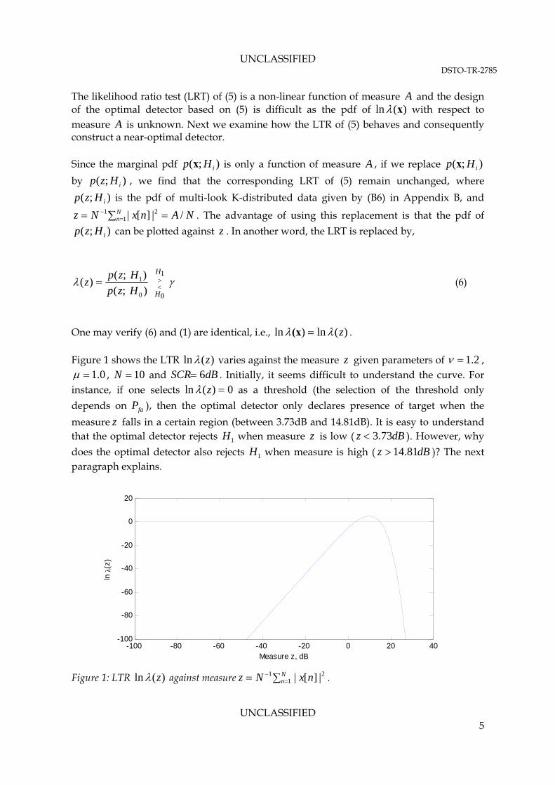
The likelihood ratio test (LRT) of (5) is a non-linear function of measure A and the design of the optimal detector based on (5) is difficult as the pdf of )x(ln with respect to measure is unknown. Next we examine how the LTR of A (5) behaves and consequently construct a near-optimal detector. Since the marginal pdf is only a function of measure A , if we replace
by , we find that the corresponding LRT of
);( iHp x
N/
z
);( iHp x
);( iHzp
); iHz
N Nn |1
1
); iHz
(5) remain unchanged, where
is the pdf of multi-look K-distributed data given by (p
z
(p
(B6) in Appendix B, and
. The advantage of using this replacement is that the pdf of
can be plotted against . In another word, the LRT is replaced by,
Anx |][ 2
0
1
);(
);()(
0
1
H
H
Hzp
Hzpz
(6)
One may verify (6) and (1) are identical, i.e., )(ln)ln z (x . Figure 1 shows the LTR )(ln z varies against the measure given parameters of z 2.1 ,
0.1 , and . Initially, it seems difficult to understand the curve. For instance, if one selects
10N dBSCR 6)(ln z 0 as a threshold (the selection of the threshold only
depends on ), then the optimal detector only declares presence of target when the
measure falls in a certain region (between 3.73dB and 14.81dB). It is easy to understand that the optimal detector rejects when measure
faP
z
1H z is low ( dBz 73.3 ). However, why
does the optimal detector also rejects when measure is high ( )? The next paragraph explains.
1H dB81z .14
-100 -80 -60 -40 -20 0 20 40-100
-80
-60
-40
-20
0
20
Measure z, dB
ln
(z)
Figure 1: LTR )(ln z against measure . N
n nxNz 121 |][|
UNCLASSIFIED 5

UNCLASSIFIED DSTO-TR-2785
Shown in Figure 2 are pdfs of multi-look clutter and multi-look target plus clutter, respectively, for the given parameters. The pdf’s are shown on linear scale and log scale, respectively. Shown in the figure is also the LTR. Now the interpretation of LTR curve becomes clear. When z value is low, is higher than , and the difference
gradually decreases with increasing in
);( 0Hzp );( 1Hzp
z , and reaches a point , where
. On the log scale, LTR monotonically increases and reaches 0 at .
After p ecomes higher than ;(zp LTR continues its monotonic increase
and reaches its peak where the ratio of the two is maximum. After that point, though );( 1Hzp igher than );( 0Hzp o decreases. The LTR curve starts dropping
from its peak till reaching 0 at 2 where again (p
1T
).
);();( 1101 HTpHTp
1T , );( 1Hz b
is still h
1T
)0H
, the rati
T
, so
; 122 HTT (); 0 pH After T ,
again becomes higher than , as the distribution of has a longer
and heavier tail, according to the given conditions. Therefore, the curve LTR monotonically decreases after it surpasses its peak.
2
);( 0Hzp );( 1Hzp ); 0Hz(p
-50 -40 -30 -20 -10 0 10 20 300
0.1
0.2
Measure z, dB
-50 -40 -30 -20 -10 0 10 20 3010
-20
10-10
100
Measure z, dB
-50 -40 -30 -20 -10 0 10 20 30-100
-50
0
Measure z, dB
ln
(z)
T1 T
2
Target + clutter
Clutter
Threshold
Figure 2: (top and middle) pdf’s of clutter and target plus clutter on linear scale and log scale,
respectively; (bottom) LTR. The region satisfying LTR greater than 0)(ln z is also shown in all three plots.
UNCLASSIFIED 6

UNCLASSIFIED DSTO-TR-2785
0)(ln zSupposing we choose a threshold, , to accept as shown. This is equivalent
we relax the optimal condition from
1
to accepting 1H when );( 11 Hzp herefore, th region ],[ 21 TT that the optimal
detector accepts 1H here the pdf of clutter plus target is higher than the pdf of clutter and ends at the point where the pdf of clutter becomes higher than the pdf of target plus clutter. It can be seen that the optimal detector does what exactly is required, because the condition );();( 011 HzpHzp does not hold for zT2 .
H
e );( 0Hzp . T
wstarts at the point
21 TTT If to to form a sub-optimal detector 1TT
Replafor accepting 1H , we need to study the ces. cing 21 TTT consequen by 1TT will theoretically increase both the false-alarm rate and the probability of detection, because,
dzHzpdzHzpPT
T
Tfa
1
2
1
00 ;; (7)
(8)
ur concern is only the increase of the false-alarm rate. For the optimal detector accepting
(9)
lternatively, the sub-optimal detector accepting for accompanies a false-alarm
(10)
order to have a reasonable value of for the optimal detector, the interval
dzHzpdzHzpPT
T
Td
1
2
1
11 ;;
O
1H for 21 TTT , the corresponding false-alarm rate is,
2
1
0;T
Tfa dzHzpP
A 1H 1TT rate of,
fafa
T
T TT
PPdzHzpdzHzpdzHzp 2
1 21
);();(; 000
In dP
012 TT , as 2 );( 1TTd dzHzpP . Because residuals of the pdf for 2Tz is very small, 1
fafa PP we generally have .
14.1 faP
For instance, for the above example, we found,
08754.0faP and 910 , and correspondingly, 9552.0dP and 10 . Therefore, relaxing the condition from 21 TTT1024.6 dP to not,
change either faP or dP for this example.
T 1T does
in practical terms,
The value of will surely depends on the parameters. However, for a common radar faP
detection problem, it often requires a small faP (usually 610 or smaller), and a reasonable
P (usually 0.5 or higher). In order to achiev 5.0);(2 T PHzp , the interval TTd e T1 1 ddz 12
UNCLASSIFIED 7

UNCLASSIFIED DSTO-TR-2785
mu value of in this region has to best not be too small. On the other hand, the
small to achieve faTT PdzHzp );(2
1 0 . As shown in the abo ple, for such conditions,
fafa PP holds cumulative distribution function (cdf) of clutter for the
ple is shown in
);( 0Hzp
ve exam
zdB
. For instance, the
above exam
other
Figure 3. According to this cdf, to achieve a false-alarm rate of 610 , the sub-optimal detector requires dBz 53.12 , 6
0 10);53.12( HdBzPr . On the
hand, the optimal detector might 5. require 12 dB52.153 to havfor a scenario. However, the
e a 3dB interval to achieve a reasonable probability of detection relaxation from the optimal condition of dBzdB 52.1553.12 to the suboptimal condition of zdB53.12 have, in a practi e-alarm rate of 610 because of 9
0 10) Pr .
cal term, fals the same ;52.15 HdB(z
0 1 2 3 4 5 6 7 8 9 10 11 12 13 14 15 16 17 18-11
-10
-9
-8
-7
-6
-5
-4
-3
-2
-1
0
1
Clutter inte
Log
10(1
-cd
f)
Figure 3: Cdf of multi-look K-distributed clutter shown as
nsity (dB)
)1(log10 cdf ( 2.1 0.1 , ,
10N ).
herefore, thT e sub-optimal detector using for detection performs, for practical cases, 1Tz
1Tidentical to the optimal detector using 2Tz provided that the condition of
012 TT is satisfied.
-optimal det
ince the suS b ector only requires , it means that the associated LTR curve 1Tz can be assumed to be monotonic for z0 e of such LTR curve is,
zz )(
. On
(11)
)0
g
The calculation of the sub-optimal
and
detector will become tractable, as the pdf’s of
are known. As explained and for simplicity, the sub-optimal detector usin(11) will simply be referred to as the optimal detector.
(p
)
; Hz
;( 1Hzpthe LTR of
UNCLASSIFIED 8

UNCLASSIFIED DSTO-TR-2785
The optimal detector of (11) applies to any shape parameter values. When thparam proaches infinity, it becomes the case of a Gaussian target embedded in Gaussian clutter. It is well-known that the LTR of
e shape eter ap
ti-look detector against K-distributed clutter has been discussed by
(11) is indeed the optimal for such a case. Since it is assumed that for the K-distributed clutter the underlying mean remains constant during the multi-look processing period, the variation of ][nx , Nn ,,1 , is therefore in fact a Gaussian random process for the processing period. This explains that the detector determined by the LTR of (11) is also optimal (in practical sense) for the K-distributed clutter whose slowly-varying component (underlying mean) is unknown but remains unchanged during the multi-look processing period. Since we also assumed that the underlying mean is spatially (from range bin to range bin) uncorrelated, and the best estimate of it therefore is the global mean. The case of spatially correlated clutter will be discussed in Section 4. Although the above derivation results in an identical optimal detector for Gaussian clutter and the compound K-distributed clutter. It has a guiding meaning in research. While the
erformance of the mulpmany researchers, here we first mathematically prove that it is also practically optimal for the compound K-distributed clutter using the Neyman-Pearson principle. It shows that detection must use the intensity data in order to obtain the optimal detection. Detection schemes using other data formats, such as amplitude, logarithm transform and so on are not optimal, and will result in some detection loss for the same false-alarm rate. Receiver operating characteristic (ROC) curves1 for the optimal detector determined by
zz )( are shown in Figure 4 and Figure 5 for various given parameters. It can be seen at for the same probability of detection, the required SCR increases substantially withth
the increasing in spikiness of sea clutter, compared to the exponential case. For instance, ase of 610faP , 5.0dP and 10for the c N , it requires a SCR=12.4dB for 2.1
compared to a SCR=3.8dB for (exponential case). It is understood that because of the spikiness, the threshold has to increase substantially in order to maintain the same false-alarm rate. re the t d in turn substantially decreas probability of detection. One way to increase the probability of detection is to increase the number of multi-looks in the non-coherent processing if possible.
The inc ase in hreshol es the
1 Conventionally, an ROC curve plots against for a given SCR. However, a plot of
against SCR for a given is also referred to as an ROC curve recently. This report adopts the
latter definition.
dP fdP dP
fdP
UNCLASSIFIED 9

UNCLASSIFIED DSTO-TR-2785
0 2 4 6 8 10 12 14 16 18 200
0.1
0.2
0.3
0.4
0.5
0.6
0.7
0.8
0.9
1
SCR, dB
P d
Exponential
= 50
= 10
= 5
= 1.2
Pfa = 10 -6
N = 4
Figure 4: ROC curves of the optimal detector determined by zz )( with and
.
610faP
4N
0 2 4 6 8 10 12 14 16 18 200
0.1
0.2
0.3
0.4
0.5
0.6
0.7
0.8
0.9
1
SCR, dB
P d
Exponential
= 50
= 10
= 5
= 1.2
Pfa = 10-6
N = 10
Figure 5: ROC curves of the optimal detector determined by zz )( with and
.
610faP
10N
UNCLASSIFIED 10

UNCLASSIFIED DSTO-TR-2785
Some ROC curves shown in Figure 5 were confirmed using Monte Carlo simulation. In the simulation, first a dataset of K-distributed clutter and a dataset of Gaussian distributed target signals, both in the complex domain, were generated according to the given parameters. The two datasets were combined together in the complex domain. After taking the square of data’s amplitude, multi-look average processing was followed. The number of measures exceeding the corresponding threshold was counted and the associated was calculated. The detection performance calculated by the Monte Carlo
simulation is shown in dP
Figure 6, together with the correspondingly theoretical ROC curves for comparison. It can be seen that they are consistent.
0 2 4 6 8 10 12 14 16 18 200
0.1
0.2
0.3
0.4
0.5
0.6
0.7
0.8
0.9
1
SCR, dB
P d
Theory, =10
Monte Carlosimulation
Theory, = 1.2
Monte Carlosimulation
Pfa=10-6
N=10
Figure 6: Confirmation of detection performance using Monte Carlo simulation.
The performance of other detectors was investigated. In particular, we take a look at two other detectors, namely, the amplitude detector using the measure of , and
the log detector using for detection, respectively. While there are
analytical forms of pdf and cdf for single-look K-distributed data when the data is measured in amplitude or in log domain (a simple pdf transform governed by
N
n nxN 11 |][|
2
1 101 |][|log10 N
n nxN
dydxxpxyp /)())(( ), the pdf and cdf of multi-look K-distributed data do not have
simple analytical forms when multi-look average processing is performed for the amplitude or in the log domain. Therefore the performance of the amplitude detector and log detector for the Gaussian target embedded in the K-distributed clutter is numerically calculated using the Monte Carlo simulation (the accuracy of the Monte Carlo simulation has been demonstrated in Figure 6). Shown in Figure 7 are ROC curves of amplitude detector and log detector in comparison with the optimal detector, i.e., the intensity detector. It can be seen that neither the amplitude nor log detectors perform as well as the optimal detector. Parameters used in the simulation are given in the figure. Other
UNCLASSIFIED 11

UNCLASSIFIED DSTO-TR-2785
parameters were also tested, and the associated ROC curves have a similar trend to the result shown in Figure 7.
0 2 4 6 8 10 12 14 16 18 200
0.1
0.2
0.3
0.4
0.5
0.6
0.7
0.8
0.9
1
SCR, dB
P d
Optimaldetection
Amplitudedetection
Logdetection
=50 =1.2
Pfa=10-6
N=10
Figure 7: Performance of amplitude detection and log detection in comparison to the optimal
detection, i.e., the intensity detection.
3.2 Clutter with Temporal Correlation
Definitions of temporal and spatial correlations as well as their calculations for the compound K-distributed clutter are discussed in Appendix C. We begin the discussion for temporal correlation in this subsection and leave the discussion for the spatial correlation to Section 4. When measure x is temporally correlated, the associated marginal pdf becomes,
xMxM
x 10 exp
det
1,; f
H
fN
Hp
(12)
xMMxMM
x12
21 expdet
1,;
sf
H
sfN
Hp
(13)
where is the normalised covariance matrix of clutter with respect to pulse, the matrix
can also be viewed as the covariance matrix of the fast-varying component of the clutter (See Appendix C for details), and is the normalised covariance matrix of target signal
with respect to pulse.
fM
sM
UNCLASSIFIED 12

UNCLASSIFIED DSTO-TR-2785
Following the derivation process shown in the previous subsection, the corresponding LTR for the model presented by (12) and (13) is,
xMxx 11)( H
N (14)
It can be denoted by,
sxx ˆ1
)( H
N (15)
where
xMs 1ˆ (16)
1211 sff MMMM (17)
The diagram of such an optimal detector is shown in Figure 8. The N-P detector correlates the received signal with an estimate of the signal . It is therefore termed an
estimate-correlator (Kay, 1998, Chapter 5), and s is usually referred to as a Wiener filter estimator of the signal.
][nx ][nsˆ
Wienerfilter
N
1'
'
H1
H0
x[n]
M-1
Figure 8: Estimate-correlator for non-coherent detection of Gaussian random signal in compound K-distributed clutter.
3.2.1 Case I: sf MM
If both clutter and target signal have the same normalised covariance matrix, , the above Wiener filter can be simplified to, 0MMM sf
1
01 MM (18)
UNCLASSIFIED 13

UNCLASSIFIED DSTO-TR-2785
This is the well-known whitening processing. The coloured (correlated) measures become white (uncorrelated) after the whitening processing. Since the data becomes uncorrelated after the whitening processing, the detection performance, including the threshold, false-alarm rate and probability of detection are all the same as those discussed in the previous subsection. 3.2.2 Case II: sf MM
Unlike clutter data, whose parameters can be measured or estimated from the secondary data, target signals are normally unknown. If there is no prior knowledge, target signals may be assumed to be uncorrelated, giving,
1211 IMMM ff (19)
The matrix inversion lemma leads to,
1
1
2111 1111
fff MIMMM
(20)
It can be seen from (20) that owing to different correlation properties of clutter and target signals, the optimal processor cannot form a filter that de-correlates correlated measurements into fully uncorrelated measurements under either or hypothesis.
Instead, the processor compromises the different correlation properties of clutter and target signal, and de-correlates measurements into overall least correlation to achieve the optimal detection. It can be shown that for a large SCR (strong target) case.
0H 1H
111 fMM Implementation of the Wiener filter (19) for the optimal processor, however, encounters a difficulty as it requires knowledge of the target signal’s intensity. Because there is no prior knowledge of target signals, such an optimal detector is difficult to implement. The generalised likelihood ratio test (GLRT) allows to be estimated by the maximised
likelihood estimate (MLE) method. The MLE of is obtained by maximising the
marginal pdf of
22
1,;lnmax2
Hp
x .
N
n
N
n n
Hn
n
cH
c
N
NHp
1 12
2
2
1221
ln)2ln(
detln)2ln(,;ln
xE
xIMxIMx
(21)
UNCLASSIFIED 14

UNCLASSIFIED DSTO-TR-2785
where fc MM , n and , nE Nn ,,1 , are the eigenvalues and eigenvectors of .
To find the MLE of , we must minimise with respect to , where
cM2 )( 2J 2
N
n n
Hn
nJ1
2
2
22 ln)(
xE
(22)
Differentiating leads to a non-linear equation of , and there is no general
solution. Therefore, the GLRT detector cannot be found analytically.
)( 2J 2
We therefore need to find suboptimal detectors. One of suboptimal detector is to use
(1fM is an arbitrary real number), because the filter fully de-correlates the clutter to
achieve the lowest threshold for a given false-alarm rate. This suboptimal detector also becomes optimal for the strong target case. Selecting 1 , the data after the whitening processing will become statistically identical to the case of uncorrelated clutter discussed in Subsection 3.1 under hypothesis , so that the threshold setting will be unchanged.
The whitening filter, however will affect the measurement of target signal which in turn alters the detection.
0H
For uncorrelated Gaussian target signal vector , the mean measurement of multi-looks is tx
2NE tHt xx . When the whitening filter is used, the measurement becomes,
N
n nftf
H
tf trE1
2212/12/1 1
MxMxM (23)
where denotes trace of matrix and tr n , Nn ,,1 , are eigenvalues of . Because fM
Nn nf Ntr 1M , we immediately have,
NN
n n
1
1
(24)
The equal sign holds if and only if 11 N
1,,0
that is for the uncorrelated case of
. Therefore, when clutter is correlated and the whitening filter is used to fully de-
correlate the correlated clutter, the whitening filter over the uncorrelated Gaussian target signal always results in a target gain. For instance, if the correlation coefficient is a geometric series, i.e., ,
IM f
nn Nn (such as )exp( nn , 0 is a
constant) then we can show,
2
21
||1
||)2(
NNtr fM (25)
UNCLASSIFIED 15

UNCLASSIFIED DSTO-TR-2785
The corresponding target signal gain will be,
)||1(
||)2(2
2
N
NNg (26)
The proof of (25) may be found in Appendix D. Therefore, the higher the correlation, the higher the target gain. The pdf of will not be gamma, and can be derived
using the method given in Appendix E if desired. tf
Htz xMx 1
The reason we obtain a target signal gain by applying the whitening filter may be explained in this way. When both target signal and clutter are uncorrelated, the intensity estimation is the only way to detect the presence of target signal. However when clutter is correlated, its spectrum is not uniformly distributed anymore, whereas the uncorrelated target signal has a uniformly distributed spectrum. In other words, the difference in spectra, if being utilised can improve the detection (or equivalently, providing a target signal gain). The function of the whitening filter in the spectral domain is to multiply a least coefficient to the largest power spectral component and a largest coefficient to the least power spectral component so that the filtered data has a uniformly distributed power spectrum. Applying the same coefficients to the uniformly distributed power spectral components (uncorrelated target signal), however, provides a gain. As an illustration, Figure 9 depicts power spectra of the correlated clutter and the uncorrelated target signal, respectively ( ). As shown in the figure, the original SCR is, 6N
5.012
6
5.05.01352
111111
SCR (27)
The whitening processing is to find a set of coefficients so that the spectrum of clutter after filtering becomes uniformly distributed while maintaining the integral of the power spectrum (the total power) unchanged. Such a set of coefficients is,
. However the same set coefficients when applied to the spectrum of uncorrelated target signal generates a gain, as the SCR after filtering processing becomes,
4423/25/21
1222222
4423/25/21
SCR (28)
Comparing (27) and (28), the generated gain is 2 (3dB). From this example, we can also see that the higher the correlation, the higher the target signal gain, as indicated previously.
UNCLASSIFIED 16

UNCLASSIFIED DSTO-TR-2785
f
f 1 f 2 f 3 f 4 f 5 f 6
5
3
2
10.50.5
PSD
(a)
f
f 1 f 2 f 3 f 4 f 5 f 6
1 1 1111
PSD
(b)
Figure 9: Power spectra of (a) correlated clutter and (b) uncorrelated target signal.
In conclusion, if target signal and clutter have different correlation properties, and there is no prior knowledge about the target signal, the GLRT detector cannot be found. One of the sub-optimal detectors for the uncorrelated Gaussian target signal embedded in the correlated K-distributed clutter is to use the inverse of the normalised covariance matrix of clutter as the whitening filter (this sub-optimal detector becomes optimal for large SCR targets). After the whitening processing, the associated threshold for a given false-alarm rate will be the same as that for the uncorrelated clutter. On the other hand, the whitening process provides a target signal gain (the value of the gain is dependent on the correlation properties of the clutter), and hence results in a higher probability of detection compared to the same target signal embedded in uncorrelated clutter. In another words, the ROC curves discussed in Subsection 3.1 is for the worst case scenario. To demonstrate, Figure 10 compares the performance of the sub-optimal detector using
as the whitening filter for detecting uncorrelated Gaussian target signals embedded
in correlated K-distributed clutter. The blue ROC curve is analytically calculated for the uncorrelated Gaussian target signal embedded in the uncorrelated K-distributed clutter with a shape parameter of
1fM
2.1 . The green asterisks are the result of the Monte Carlo simulation, which matches the theoretical results. The second ROC curve (red line with small circles) is the result of the Monte Carlo simulation for a case of the uncorrelated Gaussian target signal embedded in the correlated K-distributed clutter with the correlation coefficients of )nexp(n , 1,,0 Nn
)2/n
. The third ROC curve (broken
purple line with small circles) is the result of the Monte Carlo simulation for a case of the uncorrelated Gaussian target signals embedded in the correlated K-distributed clutter with the correlation coefficients of exp(n , 1,,0 Nn . As illustrated earlier, since
the whitening processing produces a target signal gain for the uncorrelated target signals, the detection for the two correlated clutter cases are improved. According to (26), the
UNCLASSIFIED 17

UNCLASSIFIED DSTO-TR-2785
associated target signal gains are 1.28 (1.1dB) and 2.05 (3.1dB) for the two correlated cases, respectively. Knowing the target signal gain, the associated probability of detection can also be approximately found from the probability of detection for the uncorrelated case2. For instance, the target gain for the second correlated case is 3.1dB, which means the probability of detection for a target having a SCR of 10dB for the correlated case will be close to the probability of detection for a target having an SCR of 13.1dB for the uncorrelated case, i.e., the third ROC curve can be approximately obtained by horizontally left-shifting the first ROC curve by 3.1dB. Similarly, the second ROC curve can be approximately obtained by horizontally left-shifting the first ROC curve by 1.1dB.
0 2 4 6 8 10 12 14 16 18 200
0.1
0.2
0.3
0.4
0.5
0.6
0.7
0.8
0.9
1
SCR, dB
P d
Theoretical,uncorrelated
Monte Carlo,uncorrelated
Monte Carlo,correlated I
Monte Carlo,correlated II
Figure 10: ROC comparison between uncorrelated and correlated K-distributed clutter embedded
with uncorrelated Gaussian target signals. Two correlated cases are shown: Case I with correlation coefficients of )exp( nn , 1,,0 Nn , and Case II with correlation
coefficients of )nexp(n , 1,,0 N faPn ( , 610 1 , 2.1 and
). 10N
If target signal is temporally correlated and has a normalised correlation covariance matrix
that is known a priori, the target signal mean using as the whitening filtering can
be calculated by,
sM 1f
M
22/112/12/12/1 sfstf
H
tf trE MMMxMxM
(29)
2 The pdf of the target signal after whitening processing slightly differs from the multi-look gamma distribution, resulting in a slightly different detection.
UNCLASSIFIED 18

UNCLASSIFIED DSTO-TR-2785
The corresponding target signal gain then can be calculated.
4. Detection Against Spatially Correlated Clutter
Spatial correlation is governed by the slowly-varying component of the compound K-distributed clutter. The spatial correlation is the correlation with respect to range bin, while the temporal correlation discussed earlier is the correlation with respect to pulse. Details of how to discriminate the spatial correlation from the temporal correlation, as well as how to calculate / estimate the correlation coefficients are given in Appendix C. For simplicity, the discussion in this section only considers the spatial correlation, as the temporal correlation has been discussed. The difference between Gaussian clutter and the compound K-distributed clutter lies that the texture (the mean of the slowly-varying component) is a constant for the former and fluctuates for the latter. If the local texture were known, the corresponding N-P optimal detector would be (when there is no temporal correlation),
0
1
1
2|][|11
)(H
HN
nnx
N
x (30)
where the threshold is determined by the false-alarm rate, and,
NNN
Pfa ,)(
1
(31)
ba, is the incomplete gamma function3, defined as, . The optimal
detector of
b
ta dtetba 1,
(30) can be directly derived from the pdf of multi-look uncorrelated Gaussian clutter given by (B5). The detector (30) is referred to as the ‘ideal CFAR’ (Watts 1985; Ward et al. 2006), and its performance is identical to the optimal detector discussed in Section 3 for the Gaussian clutter case. In the previous Section, the slowly-varying component (texture) is assumed to be fully-correlated (remain constant) during the multi-pulse collection for the same range bin, but fully-uncorrelated from range bin to range bin. When the local texture is spatially uncorrelated, its best estimate is its global mean . The optimal and near-optimal
3 Matlab defines the incomplete gamma function in a different way, as,
b
ta dteta
ab0
1
)(
1),( .
As a result, NNPfa ,1 .
UNCLASSIFIED 19

UNCLASSIFIED DSTO-TR-2785
processors presented in Section 3 implicitly use the global mean as the estimate of the local texture because it is the best estimate when there is no correlation. 4.1 Estimation of Local Texture
The texture of sea clutter is believed to be highly correlated to wave and swell structures of the sea (Ward et al. 2006, Chapter 2), and some waves can be metres, tens or hundreds of metres long. This leads to the slowly-varying component to be possibly spatially correlated. For spatially correlated sea clutter, the local mean estimated by the neighbouring range bins of CUT is often a better estimate than the global mean . As a consequence, using the detector (30) with the estimate as the replacement of the unknown parameter may result a better detection. This is known as the CFAR gain (Watts 1996; Watts et al. 2007; Watts 1987; Ward et al. 2006). Whether a CFAR gain is achievable depends on three conditions:
1. Clutter has fluctuating texture (i.e., compound non-Gaussian distributed); 2. The texture is spatially correlated; and
3. The local texture is estimated correctly.
The CFAR gain in turn depends on the accuracy of the estimate of the local mean , and the spikiness of the clutter. If clutter is spiky, and its spatial correlation is high, obtaining a CFAR gain is possible by a proper estimation for the local texture. It should be pointed out that the application of the above method is not limited to the case of compound K-distribution. In fact, any compound non-Gaussian distribution whose texture may have different pdfs but possess the similar characteristic (e.g., constant during the multi-pulse collection and fluctuating from range bin to range bin and spatially correlated) falls in this category. As stated above, the better the estimate of the local texture , the better the performance of the detector. Therefore, finding the ways that make better estimates of the local texture improves the performance of the detector. Following the idea given by Bucciarelli et al (1996), we use the linear autoregressive (AR) technique to estimate the local texture . Because , we can
use the clutter intensity
}{}||{}{}{ 2 ExEEzE f z to estimate the underlying texture .
UNCLASSIFIED 20

UNCLASSIFIED DSTO-TR-2785
1 L...-1-L ...
1
N
2
...
CUT
Range Range
Pu
lses
... ...
Range RangeCUT
z[0] z[L]z[1]z[-L] z[-1]
(a) Before multi-look averaging processing (b) After multi-look processing
Figure 11: Use neighbouring measures to estimate CUT (the case of multi-look in azimuth).
Figure 11 depicts the use of neighbouring cells to estimate the texture. As shown in Figure
11 (b), for a multi-look CUT 2
1 01 |][|]0[
N
iixNz , we want to use its neighbouring cells
to estimate its value. Using the AR technique, the estimate of may be expressed as a linear combination of its neighbouring cells, as (for a general stationary and symmetrical random process),
]0[z
][][]0[ˆ1
nznzwzL
nn
(32)
where is the length of the one-side estimation window. The unknown parameters, ,
, should satisfy,
L
,nw
Ln ,1
2
,,1,]0[ˆ]0[min zz
Lnwn
(33)
Among the L unknown parameters, , nw Ln ,,1 , however, only are
independent, as
1L
]n[][]0[ˆ1
znzwzL
nn
leads to,
2
11
L
nnw (34)
Without loss of generality, we rewrite (34) as,
L
nnww
21 2
1 (35)
The minimisation of (33) can be found by use of the Lagrange theorem, as,
UNCLASSIFIED 21

UNCLASSIFIED DSTO-TR-2785
kk w
zz
w
zz
]0[ˆ
]0[ˆ]0[ˆ
]0[ (36) Lk ,,2
Inserting (32) and (34) into (36), and after some manipulation, we have,
021111||2
02111222
1
kknnknkn
L
nn
kkk
w Lk ,,2 (37)
where
)var(
}{][][ 2
z
zEkizizEk
, ,1,0k , is the correlation coefficient of z .
Changing the value of k gives 1L linear equations, which provides a unique solution for , . Together with nw Ln ,,2 (35), the all unknown parameters, w , ,
can be uniquely obtained. n Ln ,,2,1
It can be shown that for spatially uncorrelated data, the weights become equal and
, . That is consistent with the well-known CA processing. If,
however, clutter is spatially correlated, the optimal weights are unequal.
)2/(1 Lwn Ln ,,1
Considering extended target signals which may occupy a few range cells, radar engineers often prefer to exclude a few guardian cells next to CUT when estimating CUT using neighbouring cells, which is shown in Figure 12. The corresponding optimal weights can be found accordingly using the following linear equations.
... ...
Range Range
CUT
z[-L-g] z[-1-g] z[0] z[L+g]z[1+g]
Guardians
Figure 12: CUT estimation using neighbouring cells with guardian cells.
022211211||22
0222111222
1
ggkkgnnkngkn
L
nn
ggkkggk
w
k (38) L,,2
where
g is the number of guardian cells at each side excluded in the estimation processing.
UNCLASSIFIED 22

UNCLASSIFIED DSTO-TR-2785
4.2 Results
After the local t
exture of CUT is estimated, we can now use the suboptimal detector,
0
1
1
2
0
|][|1
ˆ1
)(H
HN
nnx
N
x (39)
to carry out the detection, where ]0[ˆˆ0 z
However, since the pdf of
is the estimate of CUT’s texture obtained by the
reviously subsection. )(x p is unknown, the threshold for the o unkno
arlo simulation, the performance of the detector (39) is determined by e following two steps.
lly correlated K-distributed clutter data accordingly, estimating its local texture, calculating the test ratio using (39), and numerically determining
determining the probability of detection accordingly. The detection calculation used samples.
relation. elow we show two numerical samples to demonstrate the improvement of using the
me the gamma distributed clutter texture has a correlation oefficient of,
above suboptimal detector is als wn, and has to be simulated using the Monte Carlo simulation. Using the Monte Cth
1. Generating spatia
the threshold. The simulation used 910N samples to determine the threshold, which ensures an absolute relative error less than 5% for 95% of time for a false-alarm rate of 610 ( 610faP ) (Kay 1998, Chapter 2).
2. Generating clutter data, adding target signal data and
610N The detection improvement (CFAR gains achieved) varies depending on the corBoptimal weights to estimate the local texture. We assume there is no temporal correlation because such correlation can be decorrelated using the technique described in Section 3. The spatial correlation of the K-distributed clutter is resulted from the correlation of gamma distributed texture. In the first sample, we assuc
3.07.0k ,1,012/)12.0cos( kek k (40)
where denotes the number of ed rangeith the fast-varying Gaussian component, and multi-look (independent looks in azimuth)
k lagg bins. After the modulation of the texture
wintensity averaging processing, the resultant multi-look K-distributed clutter has a correlation of (refer to Appendix C for details),
UNCLASSIFIED 23

UNCLASSIFIED DSTO-TR-2785
1and10
N
Nkk
2,1k (41)
alues of 2.1V and was used in the Monte Carlo simulation. The texture
the o l weig10N
estimated by ptima hts determined by (37) is much better than the estimate of the CA window when clutter is spatially correlated. Figure 13 shows the estimates of CUT using these two methods in comparison with the true value. It can be seen that the estimates by the optimal weights follow the fluctuation much better whereas the estimates of the CA processing do not seem to follow the fluctuation closely.
0 20 40 60 80 100 120 140 160 180 200-25
-20
-15
-10
-5
0
5
10
Range bin
Clu
tter
inte
nsit
y (d
B)
Data
Estimates by optimal weights
Estimates by CA window
Figure 13: CUT estimate by use of the optimal weights and the CA window, respectively. Data
parameters are: 2.1 , 0.1 , 10N , and 8L . The spatial correlation is given by (40) and (41).
sing the optimal estimates of the texture for the suboptimal detector (39), however, did Unot show a significant improvement of the detection. A close examination indicated that small values of the estimate could lead to large values of )(x (see (39)), which, in turn, forces the threshold to be set high to maintain the desired false-alarm rate. We recall that false-alarms are often caused by sea spikes, e.g., the high clutter returns, if the detector uses a fixed threshold, and the low returns are not the concern. Therefore, it seems that there is no need for a close estimate for low clutter returns, and an accurate estimate is required only for high clutter returns. To improve the detector’s performance The estimate is modified as,
(42)
2/]0[ˆif2/
2/]0[ˆif]0[ˆˆ0
z
zz
UNCLASSIFIED 24

UNCLASSIFIED DSTO-TR-2785
The profile of the modified estimates of the clutter texture is shown in Figure 14. The modification effectively eases the false-alarms produced by low clutter returns, and hence greatly improves the detection. Our simulation indicated that the overall performance is not very sensitive to the selection of the cut-off of (for instance, (42) selects 2/ as the cut-off value). In general, a lower cut-off value improves detection a little fo w SCR targets at a small sacrifice of the detection of high SCR targets whereas a higher cut-off value improves detection a little for mid and high SCR targets at a sacrifice of the detection of low SCR targets.
r lo
0 20 40 60 80 100 120 140 160 180 200-25
-20
-15
-10
-5
0
5
10
Range bin
Clu
tter
inte
nsit
y (d
B)
Data
Modified estimatesby optimal weights
Estimates by CA window
Figure 14: Profile of the modified texture.
he performance of the suboptimal detector (39) using the modified texture estimates
Tgiven by (42) is shown in Figure 15. Compared to the fixed threshold (which assumes the mean of clutter be known), the suboptimal detector greatly improves the detection (the improvement is referred to as the CFAR gain by Watts and others (Watts 1996; Watts et al. 2007; Watts 1987)) and provides a CFAR gain about 6dB at 5.0dP . The detection using
CA processing also achieves some CFAR gain (about 2dB at 5. 0dP ), but the proposed
detector performs far better.
UNCLASSIFIED 25

UNCLASSIFIED DSTO-TR-2785
0 2 4 6 8 10 12 14 16 18 200
0.1
0.2
0.3
0.4
0.5
0.6
0.7
0.8
0.9
1
Signal-to-clutter ratio (dB)
Pro
babi
lity
of d
etec
tion
(P
d)
Optimalweights
CA window
Fixedthreshold
N=10
= 1.2Pfa = 10-6
Figure 15: ROC comparison between the fixed-threshold and the adaptive thresholds determined by
the optimal weights and a CA window with 8L for the spatially correlated K-distributed clutter with the correlation given by (40) and (41).
In the second numerical example, we assume the gamma distributed clutter texture has a correlation coefficient of,
2/kk e (43) ,1,0k
Obviously, this correlation is much lower than that of the first example. Again, the multi-look K-distributed clutter will have a correlation coefficient specified by (41). The performance of the suboptimal detector (39) using the modified texture estimate given by (42) is shown in Figure 16, together with the performances of the CA window and the fixed threshold. It can be seen that the proposed processor is still able to provide a moderate CFAR gain (about 2dB at the 5.0dP ), whereas the CA processor performs
approximately the same as the fixed threshold.
UNCLASSIFIED 26

UNCLASSIFIED DSTO-TR-2785
0 2 4 6 8 10 12 14 16 18 200
0.1
0.2
0.3
0.4
0.5
0.6
0.7
0.8
0.9
1
Signal-to-clutter ratio (dB)
Pro
babi
lity
of d
etec
tion
(P
d)
Optimal weights
CA window
Fixed threshold
N=10
= 1.2Pfa = 10-6
Figure 16: ROC comparison between the fixed-threshold and the adaptive thresholds determined by
the optimal weights and a CA window with 8L for the spatially correlated K-distributed clutter with the correlation given by (43) and (41).
It is worth noting that the achievable CFAR gain depends on the correlation and the shape parameter. The higher the correlation and smaller shape parameter, the greater the CFAR gain. If there is no correlation, there will be no CFAR gain at all. Instead, a CFAR loss will occur. Because for spatially uncorrelated clutter, the best estimate of the local mean is the global mean, and using a limited size of the CA window to estimate the local mean inherently associates with a loss (the optimal weights becomes identical to the CA window for the spatially uncorrelated clutter). ‘Ideal CFAR’ proposed by Watts (1985) is the theoretical upper bound a CFAR processor could achieve for spatially correlated non-Gaussian clutter. However, how to find the unknown ‘true’ clutter texture remains unsolved. This section uses the linear AR technique to estimate the unknown clutter texture. Theoretically, the estimate is the optimal for the given size of the window and the linear regression model. The estimated texture is then modified to mitigate possible false-alarms caused by low returns. It has shown through numerical examples, the proposed suboptimal detector is able to provide a much higher CFAR gain compared to the traditional CA processor for spatially correlated non-Gaussian clutter.
UNCLASSIFIED 27

UNCLASSIFIED DSTO-TR-2785
5. Summary
Optimal non-coherent radar detection of Gaussian targets (Swerling II model) embedded in the compound K-distributed clutter has been investigated. The derived optimal detector, under the sense of the Neyman-Pearson principle is the well-known square-law detector. This is because the underlying texture of the compound K-clutter remains unchanged during the multi-pulse averaging processing period according to the assumption, so that the clutter actually undergoes a Gaussian random process during the period of multi-pulse collection. While the derived optimal detector is not new, the derivation itself has a guiding meaning. As the detector has been rigorously derived for the first time using the Neyman-Pearson principle, it means there does not exist any detector that would perform better for the given conditions. Other detectors, such as multi-look amplitude detector, multi-look log detector and the like are inherently associated with some detection loss compared to the optimal detector, the multi-look intensity detector. A sub-optimal detector (it becomes optimal for large signal-to-clutter ratio targets) has been proposed for temporally correlated K-distributed clutter. The normalised covariance matrix of clutter is used to de-correlate the clutter. The whitening processing provides a target signal gain, resulting in an improved detection. The higher the correlation, the larger the target signal gain. The target gain results from the difference in spectra of correlated clutter and the uncorrelated target signals (a non-uniform spectrum of clutter against a uniform spectrum of target) that provides a second characteristic (in addition to the intensity) for discriminating the target from the clutter. The occurrence of uncorrelated Gaussian targets embedded in uncorrelated compound clutter represents the worst scenario in terms of detection. If the clutter is spatially correlated, using a limited number of neighbouring range bins to estimate the local texture can provide a CFAR gain and improve the detection. This report has proposed the use of the linear AR technique and derived the optimal weights for estimating the local texture of clutter. The AR estimation is optimal under the linear assumption and results in better results than the cell-averaging estimation. The AR estimates are further modified to mitigate possible false-alarms caused by low clutter returns. It has shown that the proposed processor greatly improves the detection compared to the traditional CA processor for spatially correlated clutter. The higher the correlation, the higher the CFAR gain. However, when clutter is spatially uncorrelated, the global mean is the best estimate of the local texture. A summation of the optimal or near optimal non-coherent process for detecting Gaussian targets embedded in K-distributed clutter that may be temporally and spatially correlated is provided in Appendix A as a quick reference for radar engineers implementing the detection process.
UNCLASSIFIED 28

UNCLASSIFIED DSTO-TR-2785
References Antipov, I. (1998), "Simulation of sea clutter returns", Technical Report, DSTO-TR-0679,
Defence Science and technology Organisation, Australia. Armstrong, B. C., and Griffiths, H. D. (1991), "CFAR detection of fluctuating targets in
spatially correlated K-distributed clutter", Radar and Signal Processing, IEE Proceedings F, 138(2), 139-152.
Bucciarelli, T., Lombardo, P., and Tamburrini, S. (1996), "Optimum CFAR detection against
compound Gaussian clutter with partially correlated texture", IEE Proc.~Radar, Sonar Navig., 143(2), 95-104.
Conte, E., Lops, M., and Ricci, G. (1999), "Incoherent radar detection in compound-
Gaussian clutter", IEEE Trans on Aerospace and Electronic Systems, 35(3), 790-800. Crisp, D. J., Stacy, N. J. S., and Goh, A. S. (2006), "Ingara medium-high incidence angle
polarimetric sea clutter measurements and analysis", Technical Report, DSTO-TR-1818, Defence Science and Technology Organisation, Australia.
Dong, Y. (2012), "Optimal coherent radar detection in a K-distributed clutter environment",
IET Radar, Sonar and Navig., 6(5), 283-292. Dong, Y., and Haywood, B. (2007), "High grazing angle X-band sea clutter distributions",
International Radar Conference, Edinburgh, UK. Dong, Y., and Merrett, D. (2010), "Analysis of L-band multi-channel sea clutter", IET Radar,
Sonar and Navig., 4(Iss 2), 223-238. Farina, A., Gini, F., Greco, M. V., and Verrazzani, L. (1997), "High resolution sea clutter
data: A statistical analysis of recorded live data", IEE Proceedings, Pt F, 144(3), 121-130.
Farshchian, M., and Posner, F. L. (2010), "The Pareto distribution for low grazing angle and
high resolution X-band sea clutter", IEEE International Radar Conference, Washington D.C.: 789-793.
Gini, F., Greco, M. V., and Farina, A. (1999), "Clarivoyant and adaptive signal detection in
non-Gaussian clutter: a data-dependent threshold interpretation", IEEE Trans. on Aerospace and Electronic Systems, 35(3), 1522-1531.
Gini, F., Greco, M. V., Farina, A., and Lombardo, P. (1998), "Optimal and mismatched
detection against K-distributed plus Gaussian Clutter", IEEE Trans. on Aerospace and Electronic Systems, 34(3), 860-876.
UNCLASSIFIED 29

UNCLASSIFIED DSTO-TR-2785
Greco, M. V., and Gini, F. (2007). "Sea-clutter nonlinearity: The influence of long waves", Adaptive Radar Signal Processing, S. Haykin, New York, John Wiley and Sons.
Kay, S. M. (1998), Fundamentals of Statistical Signal Processing. Vol. II, Detection Theory, New
Jersey, Prentice Hall. Rangaswamy, M., Weiner, D. D., and Ozturk, A. (1993), "Non-Gaussian random vector
identification using spherically invariant random processes", IEEE Trans. on Aerospace and Electronic Systems, 29(1), 111-124.
Sangston, K. J., and Gerlach, K. R. (1994), "Coherent detection of radar targets in non-
Gaussian background", IEEE Trans. on Aerospace and Electronic Systems, 30(2), 330-340.
Sangston, K. J., Gini, F., and Greco, M. S. (2010), "New results on coherent radar target
detection in heavy-tailed compound Gaussian clutter", IEEE International Radar Conference, Washington D.C.: 779-784.
Sangston, K. J., Gini, F., Greco, M. V., and Farina, A. (1999), "Structures for radar detection
in compound Guassian clutter", IEEE Trans. on Aerospace and Electronic Systems, 35(2), 445-458.
Ward, K. D., Tough, R. J. A., and Watts, S. (2006), Sea Clutter: Scattering, the K Distribution
and Radar Performance, London, Institute of Engineering Technology. Watts, S. (1985), "Radar detection prediction in sea clutter using the compound K
distribution model", IEE Proceedings, Pt F, 32(7), 613-620. Watts, S. (1987), "Radar detection prediction in K-distributed sea clutter and thermal
noise", IEEE Trans. on Aerospace and Electronic Systems, AES-23(1), 40-45. Watts, S. (1996), "Cell-averaging CFAR again in spatially correlated K-distributed clutter",
IEE Proc.~Radar, Sonar Navig., 143(5), 321-327. Watts, S., Ward, K., and Tough, R. (2007), "CFAR loss and gain in K-distributed sea-clutter
and thermal noise", IET International Conference on Radar Systems: 1-5. Watts, S., Ward, K. D., and Tough, R. J. A. (2005), "The physics and modelling of discrete
spikes in radar sea clutter", International Radar Conference.
UNCLASSIFIED 30

UNCLASSIFIED DSTO-TR-2785
Appendix A: Summation of Optimal or near Optimal Non-coherent Detection Process
This appendix is a summation of the optimal or near optimal non-coherent radar process discussed in this report. It serves as a quick reference for radar engineers implementing the detection process. Assumptions:
1. Clutter has a compound K-distribution (thermal noise is included), and may have temporal correlation (with respect to pulse) and spatial correlation (with respect to range). Parameters of the K-distribution as well as the correlations are known or have been estimated using the sample data.
2. Target is point-like and has a Gaussian distribution.
For each cell under test (CUT), its neighbouring cells under the consideration is depicted in Figure A1. The neighbouring cells under the consideration are assumed to be target-free. CUT
1 L...-1-L ...
1
N
2
...
Range Range
Pu
lse
Guardians
0g g
Figure A1: Using neighbouring cells to estimate CUT (the case of multi-look in pulse and multi-look in range).
First, the temporal correlation is decorrelated and cell values are averaged for each range bin. This process is called multi-look process.
lHll N
z xMx 1
(A1) Ll ,,1
where
UNCLASSIFIED 31

UNCLASSIFIED DSTO-TR-2785
Tlll Nxx ][]1[ x (A2)
The calculation of is given by 1M (20). If target signal is uncorrelated or unknown, becomes,
1M
111 fMM (A3)
where is the clutter mean and is the normalised temporal correlation matrix of
clutter. If clutter is temporally uncorrelated, (A1) becomes, fM
N
nll nx
Nz
1
2][
1 (A4) Ll ,,1
The above process reduces the two-dimensional data window to a one-dimensional data window as shown in Figure A2.
... ...
Range Range
CUT
z[-L-g] z[-1-g] z[0] z[L+g]z[1+g]
Guardians
Figure A2: Data window after multi-look processing.
The second stage is to estimate by symmetrical weights, as, ]0[z
L
nn nznzwz
1
][][]0[ˆ (A5)
The weights are calculated by,
LLLL
L
L b
b
aa
aa
w
w
w
2
1
2
2222
1 2/1
0
0
111
(A6)
Where
0222111222
1 ggkkggkkb Lk ,,2 (A7)
UNCLASSIFIED 32

UNCLASSIFIED DSTO-TR-2785
022211211||2 ggkkgnnkngknkna Lnk ,,2, (A8)
where
)var(
][][ 2
z
zEkizizEk
, ,1,0k is the spatial correlation coefficient of z, and
g is the number of guardian bins on each of side of CUT. The correlation is assumed to be symmetrical with respect to CUT. Finally we calculate 0 by,
2/]0[ˆif2/
2/]0[ˆif]0[ˆˆ0
z
zz (A9)
The detection is then performed simply by comparing /0ˆ to a threshold that is
determined by the false-alarm rate to declare absence or presence of target in the CUT. The whole detection process is depicted in Figure A3.
Multi-look processin azimuth
Weighted averagein range
z[l]x [n]l
z[0]
H1
H0
> m/2
<= m/2
t0^
-.. Figure A3: Block diagram of optimal or near optimal non-coherent detection of Gaussian targets embedded in compound K-distributed clutter.
If we let L
w , n , then the spatial processing becomes cell-average CFAR
(CA-CFAR) in range. If there is no spatial correlation (correlation in range), there is no need to estimate z using multiple range cells. The best estimation of z is
n 2
1 L,,1
]0[ ]0[ in this case.
UNCLASSIFIED 33

UNCLASSIFIED DSTO-TR-2785
This page is intentionally blank
UNCLASSIFIED 34
UNCLASSIFIED DSTO-TR-2785
Appendix B: Approximation of Gaussian Signal Added in K-distributed Clutter
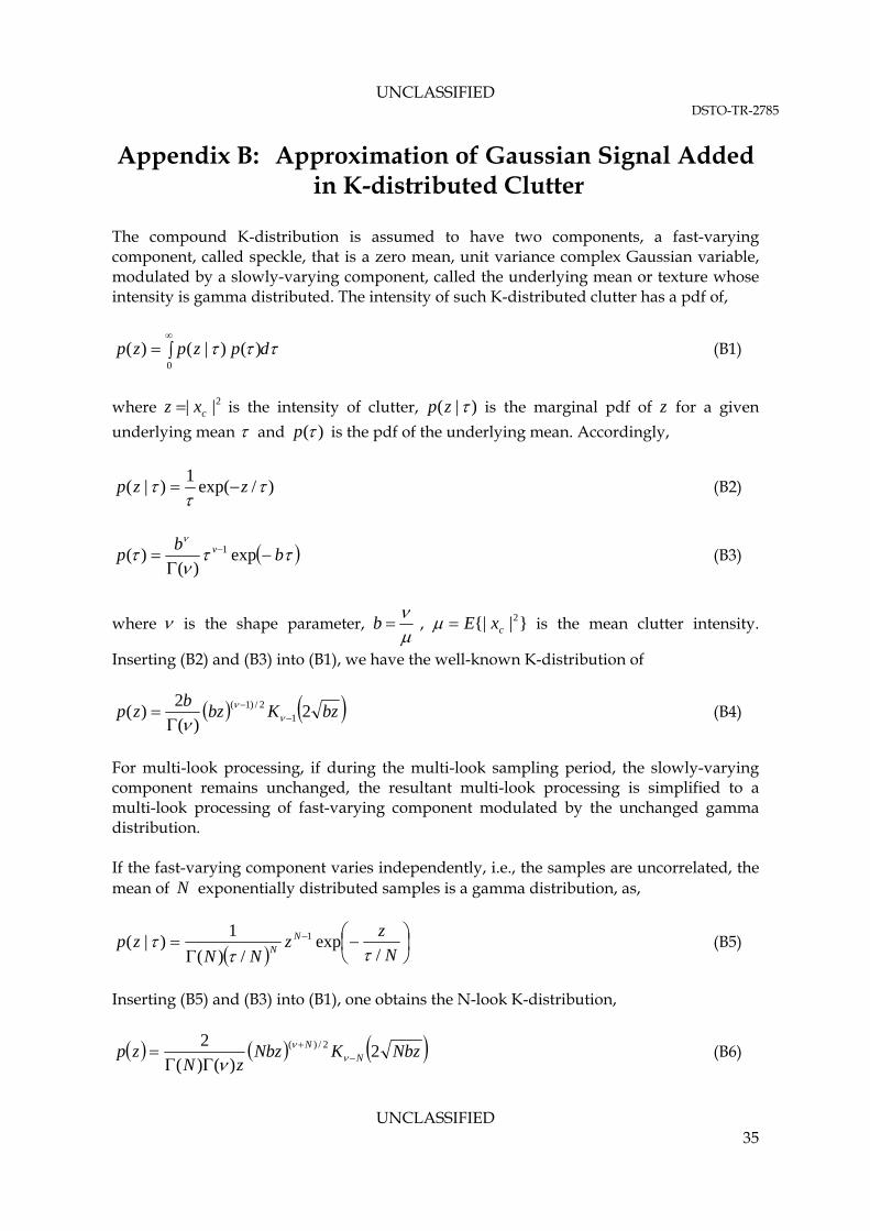
The compound K-distribution is assumed to have two components, a fast-varying component, called speckle, that is a zero mean, unit variance complex Gaussian variable, modulated by a slowly-varying component, called the underlying mean or texture whose intensity is gamma distributed. The intensity of such K-distributed clutter has a pdf of,
dpzpzp
0
)()|()( (B1)
where is the intensity of clutter, 2|| cxz )|( zp is the marginal pdf of z for a given
underlying mean and )(p is the pdf of the underlying mean. Accordingly,
)/exp(1
)|(
zzp (B2)
bb
p v
exp)(
)( 1 (B3)
where is the shape parameter,
b , is the mean clutter intensity.
Inserting
}|{| 2cxE
(B2) and (B3) into (B1), we have the well-known K-distribution of
bzKbzb
zp 2)(
2)( 1
2/)1(
(B4)
For multi-look processing, if during the multi-look sampling period, the slowly-varying component remains unchanged, the resultant multi-look processing is simplified to a multi-look processing of fast-varying component modulated by the unchanged gamma distribution. If the fast-varying component varies independently, i.e., the samples are uncorrelated, the mean of exponentially distributed samples is a gamma distribution, as, N
N
zz
NNzp N
N /exp
/)(
1)|( 1
(B5)
Inserting (B5) and (B3) into (B1), one obtains the N-look K-distribution,
NbzKNbzzN
zp NN 2
)()(
2 2/)(
(B6)
UNCLASSIFIED 35

UNCLASSIFIED DSTO-TR-2785
where
N
nnz
Nz
1][
1. When , 1N (6) simplifies to (B4).
Now consider the distribution of a combination of thermal noise (or in general a Gaussian signal) and K-distributed clutter. Assuming the Gaussian signal, and clutter each is independently random process, we denote Gaussian signal , and the
conditional clutter
),0(~ 2CNX t
),0(~| CNX c . Since they are independent processes, and is
independent of tX
, we have,
2,0~|)( CNXX ct (B7)
or,
2
121 exp
1)|(
y
z
yyzp (B8)
where 2
1 ct xxz is the intensity. The pdf of is given by, 1z
011 )()|()( dpzpzp (B9)
Unfortunately, the above integral does not have a closed-form solution. Therefore, the distribution of the Gaussian target signals (or Gaussian noise) embedded in the K-distributed clutter is unknown. For extreme cases we note that the distribution will still be the K-distribution for a very low SCR case and exponential for a high SCR case. The latter is also a K-distribution with the shape parameter of infinity. Watts (1987) has studied the distribution of the combined K-distributed clutter plus Gaussian thermal noise. He has approximated the combined distribution as a new K-distribution, with a modified shape parameter and a modified mean. Following this idea, we approximate the distribution of (B9) to a K-distribution with new parameters of 11, whose values are derived using moment methods in the following. It is known that for the K-distribution given by (B4), the shape parameter is a function of the normalised moments. For instance, for the second normalised moment,
}{
}{)1(2
12
21
1
1
zE
zE
(B10)
where , once and are found, the corresponding 2
1 || ct xxz }{ 1zE }{ 21zE 1 can be
derived accordingly, as the distribution of is assumed to be K. 1z
22221 }||{}|{|}|{|}{ ctct xExExxEzE (B11)
UNCLASSIFIED 36

UNCLASSIFIED DSTO-TR-2785
To find the variance of , we first find, 1z
}|{|}||{4}|{|}|{|}|{|}{ 2244421 ctctct xExExExExxEzE (B12)
44 2}|{| txE (B13)
24 )1(2}|{|
vxE c
(B14)
Inserting (B11)-(B14) into (B10), we have,
21 1 (B15)
where is the SCR of the data. Equation /2 (B15) is identical to what is given by Watts (1987)4. Similarly, the third normalised moment of K-distribution is,
}{
}{)1)(2(6
13
31
21
11
zE
zEv
(B16)
After some elementary algebra, (B16) becomes,
1)1(
3/)1(3/)1)(2(233
322
21
1
(B17)
When 0 , (B17) is a quadratic equation of the unknown 1 which is solvable once the shape parameter of clutter, , and the SCR, , are given. Its explicit solution is,
A
A
2
8931
(B18)
where 3)1(
2)1(3
A
We thus have derived two Formulae, i.e., (B15) and (B18) for estimating the shape parameter . If the distribution of target embedded in clutter is exactly a K-distribution, the two formulae should result in an identical value. Since the true distribution of the combined two is unknown, and the K-distribution is only an approximation, the shape 4 It is noted that in the Watts’ paper (1987), the clutter-to-noise ratio (CNR) is used whereas here the signal-to-clutter ratio (SCR) is used.
UNCLASSIFIED 37

UNCLASSIFIED DSTO-TR-2785
parameter estimated by (B15) and (B18) may be slightly different. Often(B18) results in a slightly smaller value, and the corresponding distribution may fit marginally better in the tail region. The accuracy of using a new K-distribution to approximate the distribution of Gaussian target signals embedded in K-distributed clutter may be examined by comparison between the pdf numerically integrated by (B9) (treated as the ‘true’ distribution when the integration interval is sufficiently small) and the pdf of the K-distribution whose shape parameter is determined by (B15) or (B18). Figure 17 shows such a comparison. It can be seen from the figure that the K approximation is almost identical to the true distribution, though the upper tails of the two separate apart slightly at the far end. However, the accuracy of using a new K distribution to approximate the distribution of Gaussian target signals embedded in K-distribution clutter would be sufficient for the purpose of radar detection analysis.
-30 -20 -10 0 10 200
0.02
0.04
0.06
0.08
0.1
Intensity (dB)
Numericalintegration
K approxi-mation
-100 -80 -60 -40 -20 0 20
10-10
10-5
100
Intensity (dB)
Numericalintegration
K approxi-mation
(a) pdf on linear scale (b) pdf on log scale
Figure 17: Pdf comparison between numerically integrated (viewed as ‘true distribution’) and the K approximation ( 0.1 , 0.1 and dBSCR 5 ) The shape parameter 1 is determined by (B18).
The Monte Carlo simulation was further used to examine the agreement between the assumed distribution and the actual distribution of target plus clutter. In the simulation, 10 million ( ) samples were generated, and the histograms of data were compared with the pdf of the K-distribution.
710Figure 18 and Figure 19 show the goodness-of-fit of the
histograms of data and the pdfs of the corresponding K-distributions. It can be seen that agreement between the two is superior, and hence the distribution of a Gaussian target embedded in K-distributed clutter can be confidently modelled as a new K-distribution.
UNCLASSIFIED 38

UNCLASSIFIED DSTO-TR-2785
-40 -30 -20 -10 0 10 200
0.02
0.04
0.06
0.08
0.1
Intensity (dB)
Simulated data, target+clutter
Simulated data, clutter
K-distribution of (, )
K-distribution of (1, 1
)
(a) Pdf on linear scale to show the global goodness-of-fit
-100 -80 -60 -40 -20 0 2010
-8
10-6
10-4
10-2
100
Intensity (dB)
Simulated data, target + clutter
Simulated data, clutter
K-distribution of (, )
K-distribution of (1, 1
)
(b) Pdf on log scale to show the goodness-of-fit for tails
Figure 18: Goodness-of-fit for distribution of Gaussian target embedded in K-distributed clutter ( 0.1 , 2.1 , ). dBSCR 3
UNCLASSIFIED 39

UNCLASSIFIED DSTO-TR-2785
-40 -30 -20 -10 0 10 20 300
0.02
0.04
0.06
0.08
0.1
Intensity (dB)
Simulated data, target + clutter
Simulated data, clutter
K-distribution of (, )
K-distribution of (1, 1
)
(a) Pdf on linear scale to show the global goodness-of-fit
-100 -80 -60 -40 -20 0 2010
-8
10-6
10-4
10-2
100
Intensity (dB)
Simulated data, target + clutter
Simulated data, clutter
K-distribution of (, )
K-distribution of (1, 1
)
(b) Pdf on log scale to show the goodness-of-fit for tails
Figure 19: Goodness-of-fit for distribution of Gaussian target embedded in K-distributed clutter ( 0.1 , 2.1 , ). dBSCR 10
It is found that once a Gaussian target is embedded in the K-distributed clutter, the distribution of the combined two becomes much less spikier than the original K-distributed clutter, i.e., the new shape parameter 1 is usually larger than . If SCR is large, the combined distribution approaches Gaussian (the intensity approaches exponential), as the combined signal has a dominant Gaussian component. For numerical calculations, the K-distribution with a shape parameter can be approximated as a Gaussian distribution (exponential distribution for the intensity).
50Figure 20 shows the
shape parameter 1 as a function of and SCR. If can be see that for moderate sea clutter having a shape parameter of 5 or larger, the distribution of Gaussian target plus clutter can be treated as Gaussian distributed once the SCR is greater than 3dB. However, for spikier
UNCLASSIFIED 40

UNCLASSIFIED DSTO-TR-2785
sea clutter with a shape parameter less than 1, the distribution of the combined two slowly approaches Gaussian only when SCR close or greater than 10dB.
-10 -8 -6 -4 -2 0 2 4 6 8 100
10
20
30
40
50
SCR (dB)
Sha
pe p
aram
eter
1
= 0.5
= 1.2
= 5.2
= 10.2
Figure 20: Shape parameter 1 rapidly increases with the increase in SCR (solid-line and broken-line curves are calculated by (B15) and (B17), respectively).
Another way to examine whether a distribution is exponential is to examine its statistical properties including mean, median, variance, skewness and kurtosis. Table A1 lists these statistical measures for the Monte Carlo simulated 10 million ( ) samples of Gaussian target embedded in the K-distributed clutter. It shows that with an increase in SCR, the distribution of the combined signal intensity indeed approaches exponential.
710
Figure 21 examines the goodness-of-fit for a case of Gaussian target embedded in the K-distributed clutter, with parameters of 0.1 , 0.5 , dBSCR 4 . It shows that the distribution is almost identical to the exponential distribution. Table A1: Statistical measures of Monte Carlo simulation (106 samples) in comparison with
theoretical values of an exponential distribution.
Mean Median Variance Skewness Kurtosis Exponential distribution
/)/exp()( zzp
(1.000) )2ln(
(0.6931)
2
(1.000)
2 6
10 million samples of combined target + clutter,
,5 dBSCR 4
1.000 0.686 1.032 2.097 6.821
10 million samples of combined target + clutter,
,5 dBSCR 10
1.000 0.692 1.004 2.014 6.107
UNCLASSIFIED 41

UNCLASSIFIED DSTO-TR-2785
-30 -25 -20 -15 -10 -5 0 5 10 15 200
0.02
0.04
0.06
0.08
0.1
Intensity (dB)
Simulated data, target + clutter
K-distribution
Exponential distribution
(a) Pdf on linear scale to show the global goodness-of-fit
-80 -70 -60 -50 -40 -30 -20 -10 0 10 20 3010
-10
10-8
10-6
10-4
10-2
100
Intensity (dB)
Simulated data, target + clutter
K-distribution
Exponential distribution
(b) Pdf on log scale to show the goodness-of-fit for tails
Figure 21: Goodness-of- in K-distributed clutter fit for distribution of Gaussian target embedded ( 0.1 , 0.5 , dBSCR 4 ). The approximated K-distribution is almost identical to on is the exp ential d tribution.
UNCLASSIFIED 42

UNCLASSIFIED DSTO-TR-2785
Appendix C: Temporal and Spatial Correlations of Compound K-Distributed Clutter
The compound K-distribution assumes that the data consists of a fast-varying component modulated by a slowly-varying component. The fast-varying component commonly refers to the speckle component that is a Gaussian random process with zero mean and unit variance. The slowly-varying component is also called underlying mean whose intensity has a gamma distribution. Because of the nature of these two components, caution has to be exercised when estimating temporal correlation and spatial correlation. C.1. Temporal Correlation (Correlation in Azimuth)
It often needs to know the temporal correlation between data samples collected by a pulse train in a coherent processing interval (CPI). Often we can assume during the CPI, the slowly-varying component remains unchanged, i.e., the slowly varying component is fully correlated (this is how the compound K-distributed clutter got its name)5. The covariance matrix of the data is written as,
HE xxM (C1) where expectation is with respect to the pulse for the temporal correlation, and
is a vector collected by pulses. Each measurement may be further written as a product of fast-varying and slowly-varying components, according to the model assumption, as,
TNxx ]1[]0[ x 1N N
][][ nxnx f (C2)
where is the fast-varying component which is a complex Gaussian variable, ][nx f is the
underlying mean which is constant in a CPI. Because two components are independent, we have,
fHff
H EEE MxxxxM (C3)
where H
fff E xxM is the covariance matrix of the fast-varying component and the
clutter mean. Therefore, the temporal correlation can be estimated using data samples and the correlation of fast-varying component is just the covariance matrix normalised by its mean. Under the assumption of wise sense stationary, has a Toeplitz structure of, fM
5 With reference to a maritime search radar, there is high superposition of antenna footprints with respect to successive pulses in a CPI, so the texture of sea clutter can be assumed to be completely correlated.
UNCLASSIFIED 43

UNCLASSIFIED DSTO-TR-2785
1
1
1
*1
*1
1
*1
11
N
N
fM (C4)
where ][][1 * kixixEk
, 1,,1,0, Nki .
C.2. Spatial Correlation (Correlation in Range)
The correlation of texture may be found from the spatial correlation. However in order to find the correlation of texture, we normally need to manipulate data in the intensity (or amplitude) domain rather than the complex (IQ) domain. Because if we consider the correlation between range bin and range bin i ki , 0k 6,
][][][][][][][][ ** kixixEkiiEkixkiixiE ffff (C5)
However, if the interval between bin i and bin ki is greater than the radar range
resolution, 0][][ * kixixE ff . Therefore, even if 0][][ kiiE , its value is not
measurable using the IQ data. Therefore, the correlation of texture has to be found using the intensity (or amplitude) data. First we define the correlation coefficient of texture, , and the correlation coefficient of intensity, , respectively, as,
)var(
][][ 2
EkiiE
k
(C6) ,1,0k
)var(
][][ 2
z
zEkizizEk
(C7) ,1,0k
Obviously,
100 (C8)
Below we will find the relationship between k and k for 0k .
Denoting , we have, ff zxxz 22 ||||
6 In order to simplify symbols, the same index notation is used to represent either temporal series (the index refers to pulse numbers) or spatial series (the index refers to range bin number). There should be no confusion under the context.
UNCLASSIFIED 44

UNCLASSIFIED DSTO-TR-2785
][][][][][][ kizizkiiEkiziz ffE (C9)
ince the fast-varying and slowly varying components are independent, we have, S
][][][][][][][][ kizizEkiiEkizizkii ffffE (C10)
or , the value of 0k ][][ kizizE ff F can be calculated by the Isserlis’ Theorem (see
alow ls, J.M., BucholMich icz, J.V., Nicho tz, F., and Olson, C.C., “An Isserlis’ theorem for mixed Gaussian variables: application to the auto-bispectral density”, J. Statistical Phys., 2009, 136, (1), pp. 89–102, for details), as,
][][][][][][][][1
][][][][][][
****
**
kixixEkixixEkixixEkixixE
kixkixixixEkiziz
ffffffff
fffff f
E for 0k
(C11)
the interval between bin and bin
i ki o, s
If is greater than the radar range resolution, the last two items of (C11) become zer o 1][][ kizizE ff , the above correlation
simplifies to, ][][][][ kizizEkii E for 0k (C12)
ombining (C6), (C7) and (C12), and noticing }{}{ zEEC , one achieves,
)var(
)var(
zkk
2,1k (C13)
quations (C8) and (C13) indicate once we know the correlation of z or E , the correlation
he texture
of the other can be determined.
T is gamma distributed, and the intensity is single-look or multi-look
(C14)
z(multi-pulses) K-distributed, their variances, respectively, are,
/) 2var(
21)var(
N
Nz
(C15)
here is the number of multi-looks (multi-pulses). Therefore, because of the effect of w N
the fast-varying component that is uncorrelated and randomly varies, the correlation of the intensity z is generally weaker than the correlation of the texture that is the originator of the correlation. Only if the number of multi-looks reaches infinity when the fluctuations of the fast-varying component disappears (averaged to its mean value for every range bin), two correlations become identical.
UNCLASSIFIED 45

UNCLASSIFIED DSTO-TR-2785
Inserting (C14) and (C15) into (C13), we have,
1
N 2,1k (C16) Nkk
The correctness of timulation, we first generated the slowly varying component, gamma, that has a shape
he above derivation is confirmed by the Monte Carlo simulation. In the sparameter of 2.1 and a correlation coefficient of,
12/)12..07.0 kk ek ,1,0k 0cos(3 (C17)
The multi-look K distributed data was then gulti-look fast-varying Gaussian component to the correlated gamma. The correlation
enerated by modulating the uncorrelated
mcoefficient for the simulated multi-look K data was regressed and compared to the theoretical value, and details are shown in Figure 22. It can be seen that the simulated results match the theory. Only when the number of multi-looks in the averaging processing (multi-pulse averaging processing) becomes large, the correlation of the multi-look data approached the correlation of the slowly-varying component.
0 20 40 60 800
0.2
0.4
0.6
0.8
1
0 20 40 60 800
0.2
0.4
0.6
0.8
1
Number of lagged range bin
Cor
rela
tion
coe
ffic
ient
Simulated
Number of lagged range bin
Cor
rela
tion
coe
ffic
ient
Theoretical
Simulated
Theoretical
(a) Correlation of gamma (b) correlation of K
Figure 22: (a) the designated correlation of the amma component and (b) the correlation of the m es of 1-look and 16-looks are sh
or range over-sampled data, when the range interval between bin and bin (
gulti-look K data (the cas own).
i ki 0k ) smaller than the range resolution, the fast-varying component is
Fis also correlated in range, resulting in 1][][ kizizE ff (see (C11)). So the correlation of the intensity z w
jointly contributed by the fast-varying component and the slowly-varying component.
ill be
UNCLASSIFIED 46

UNCLASSIFIED DSTO-TR-2785
Appendix D: Inverse of Covariance Matrix
Suppose a covariance matrix is symmetrical, positive definite and has a Toeplitz structure of,
1
1
1
1
*1
*2
*1
1*1
*2
21*1
121
N
N
N
N
M (D1)
The inverse, while still be symmetrical and positive definite, does not in general have a specific structure. However, if k is a geometric series, e.g., 1,,0 Nk
1)()(
1)(
1
1
**2*1
**2
2*
12
N
N
N
N
M (D2)
Then the inverse of has a simple structure as, M
ac
cbc
cbc
ca
*
*
*
1
00
0
0
00
M (D3)
where
2
2
2
2
||1
||1
||1||1
1
c
b
a
(D4)
UNCLASSIFIED 47

UNCLASSIFIED DSTO-TR-2785
To prove (D3), we denote for element of , jiA , A Nji ,1, , and
ac
cbc
cbc
ca
N
N
N
N
*
*
*
**2*1
**2
2*
12
00
0
0
00
1)()(
1)(
1
1
A (D5)
It is not difficult to write,
)Hermittianis(0
,0
1,,2,1
1,1
*,,
*21*11,
**,
*,
*1,1
AjiAA
jicbccbcA
NicbcA
acAcaA
ijji
ijijijijji
ii
NN
(D6)
UNCLASSIFIED 48

UNCLASSIFIED DSTO-TR-2785
Appendix E: Distribution of Muli-look Correlated K-Distributed Data
Multi-look processing, coherently or non-coherently, is a common practice for radar data processing. In some cases, data are correlated. We want to derive the distribution (pdf and cdf) of multi-look correlated data, including Gaussian and K-distributed data. Denoting the normalised covariance matrix of correlated complex Gaussian vector x , the correlation can be expressed by spherically invariant random process (SIRP) (
M
Rangaswamy et al. 1993; Antipov 1998). Letting t be a mutually uncorrelated circularly complex Gaussian vector with vector zero mean and covariance matrix of ( is an elementary matrix), the correlated Gaussian vector may be written as,
I2 Ix
tMx 2/1 (E1)
where , E and are eigenvectors and eigenvalues of M (note that is a Hermitian matrix, e.g., symmetrically positive definite matrix, and in addition it has a Toeplitz structure). Obviously the covariance matrix of x is,
HEEΛM 2/12/1 Λ M
MMttMxx 22/12/1 )( HHH EE (E2)
So the normalised covariance matrix is HE xxM2
1
, and . Now we
want to derive the pdf of
}||{ 22 xE
2
1 |][|1
Ni ix
N= xxH
N
1. First we have,
N
iii
N
iii
HH tktNNN 1
2
1
22/12/1 ||||1
)()(11 tMtMxx (E3)
where Nk ii / and i , , are the eigenvalues of M . Note that , ,
are mutually uncorrelated and each is a complex Gaussian distributed, and is
exponentially distributed and has a mean of .
Ni ,,1 it Ni ,,12|| it
2
According to (E3), the pdf of 2
1 |][|1
Ni ix
N is identical to the pdf of . Since
( ) are mutually uncorrelated, the pdf of can be derived from the
so-called convolution formula (Wilks, 1962, p. 204) of,
21 |][|
Ni i itk it
Ni ,,1 21 |][|
Ni i itk
dxxpxtptp N
t
N )()()( 10
(E4)
UNCLASSIFIED 49

UNCLASSIFIED DSTO-TR-2785
where . Using )()( 1 xpxp (E4), we derive the pdf of Ni
H ixNN
t 12|][|
11xx as,
N
iN
imm
mi
iNi
N
kk
ktktp
1
1
22
2
)(
)/(exp1)(
(E5)
The cdf is,
N
iN
imm
mi
iNi
N
kk
ktktp
1
1
21
)(
)/(exp1)(
(E6)
The moment of t is, thn
N
iN
imm
mi
nNinn
kk
kntE
1
1
12
)(! (E7)
It is known that the multi-look uncorrelated Gaussian data has a gamma distribution of,
N
zz
NNzp N
N /exp
/)(
1)(
21
2 (E8)
where
N
inx
Nz
1
2|][|1
, and is the number of multi-looks. N
The distribution of multi-look correlated Gaussian data is given by (E5) which is not a gamma distribution. However, for simplification, it may be approximated by a gamma distribution whose mean and equivalent number of independent looks may be found by equating the mean and the variance of the both distributions. In general, the equivalent number of independent looks is greater than 1 (fully correlated case) and less than N (fully uncorrelated case). For example, if the covariance matrix has a Toeplitz structure, as,
1
1
1
1
*1
*2
*1
1*1
*2
21*1
121
2
N
N
N
N
M (E9)
UNCLASSIFIED 50

UNCLASSIFIED DSTO-TR-2785
By equating the first and second moments of (E5) and (E8), we found the equivalent number of independent looks to be,
1
1
2||)(2
1N
nnnN
N
N
(E10) 2N
Figure 23 compares the exact distribution and the approximated gamma distribution for multi-look of Gaussian distributed data with 8N , and correlation coefficients of
)exp( nn . It can be seen that that approximated gamma distribution starts deviating
from the exact distribution in the far upper tail region.
-5 0 5 100
0.05
0.1
0.15
0.2
0.25
0 2 4 6 8 10
-5
-4
-3
-2
-1
0
T(z) in dB
log 10
(1-c
df)
(a) pdf ( )exp( nn ) (b) 1-cdf ( )exp( nn )
Figure 23: Distribution of is approximated as a gamma distribution when samples are correlated. The blue dots represent data’s distribution and the green lines stand for the approximated gamma distribution (
N
i ixNt 121 |][|
8N , )exp( nn which result in
3102.6 ).
The distribution of multi-look correlated K-distributed data can be derived in the similar way. We assume that the slowly-varying component remains constant during the multi-look process, i.e., the slowly-varying component is fully correlated during the period of multi-looks and the fast-varying component is partially correlated and has the covariance matrix of . The corresponding pdf and cdf are given by M (E11) and (E12), respectively.
N
i iv
iN
immmi
Ni z
k
bKz
k
b
kk
kbzp
11
2/)1(
,1
2
2)()(
2)(
(E11)
N
i iv
iN
immmi
Ni z
k
bKz
k
b
kk
kzP
1
2/
,1
1
22)()()(
1)(
(E12)
UNCLASSIFIED 51

UNCLASSIFIED DSTO-TR-2785
where . Similarly the exact distribution given by N
i ixNz 121 |][| (E11) can be
approximated by a multi-look K-distribution given by (B6) with an equivalent number of independent looks. Figure 24 compares the exact distribution and the approximated distribution for multi-look of K-distributed data with 8N , and correlation coefficients of )exp( nn . Although the correlation is the same as the above example, the
approximated pdf now demonstrates much better agreement with the exact pdf. Because for the K-distribution, its upper tail is primarily determined by the shape parameter (the slow-component), and the approximation processing only affects the fast-varying component, but has no effect on the slowly-varying component. As a result, the approximation for the K-distribution is better for small shape parameters than larger ones.
UNCLASSIFIED 52

UNCLASSIFIED DSTO-TR-2785
UNCLASSIFIED 53
-30 -20 -10 0 10 200
0.02
0.04
0.06
0.08
0.1
Normalised intensity (dB)
Data
Precise
Approximate
(a) pdf on linear scale
-70 -60 -50 -40 -30 -20 -10 0 10 2010
-8
10-6
10-4
10-2
100
Normalised intensity (dB)
on
log
scal
e
Data
Precise
Approximate
(b) pdf on log scale
-20 -15 -10 -5 0 5 10 15 2010
-10
10-8
10-6
10-4
10-2
100
Normalised intensity (dB)
1-cd
f on
log
scal
e
Precise
Approximate
(c) 1-cdf on log scale
Figure 24: An example of multi-correlated-look K-distribution, 8N , and nn e 2.1 . The
equivalent uncorrelated look number is 3102.6 for the approximate multi-look K distribution.

Page classification: UNCLASSIFIED
DEFENCE SCIENCE AND TECHNOLOGY ORGANISATION
DOCUMENT CONTROL DATA 1. PRIVACY MARKING/CAVEAT (OF DOCUMENT)
2. TITLE Optimal Detection in the K-Distributed Clutter Environment -- Non-Coherent Radar Processing
3. SECURITY CLASSIFICATION (FOR UNCLASSIFIED REPORTS THAT ARE LIMITED RELEASE USE (L) NEXT TO DOCUMENT CLASSIFICATION) Document (U) Title (U) Abstract (U)
4. AUTHOR(S) Yunhan Dong
5. CORPORATE AUTHOR DSTO Defence Science and Technology Organisation PO Box 1500 Edinburgh South Australia 5111 Australia
6a. DSTO NUMBER DSTO-TR-2785
6b. AR NUMBER AR-015-478
6c. TYPE OF REPORT Technical Report
7. DOCUMENT DATE December 2012
8. FILE NUMBER eg: 2009/1034056
9. TASK NUMBER CDG 07/040
10. TASK SPONSOR DGAD
11. NO. OF PAGES 53
12. NO. OF REFERENCES 26
13. DSTO Publications Repository http://dspace.dsto.defence.gov.au/dspace/
14. RELEASE AUTHORITY Chief, Electronic Warfare and Radar Division
15. SECONDARY RELEASE STATEMENT OF THIS DOCUMENT
Approved for public release OVERSEAS ENQUIRIES OUTSIDE STATED LIMITATIONS SHOULD BE REFERRED THROUGH DOCUMENT EXCHANGE, PO BOX 1500, EDINBURGH, SA 5111 16. DELIBERATE ANNOUNCEMENT No Limitations 17. CITATION IN OTHER DOCUMENTS Yes 18. DSTO RESEARCH LIBRARY THESAURUS Optimal Detection; K-Distribution; Non-Coherent Radar Processing. 19. ABSTRACT Non-coherent detection of Gaussian targets (Swerling II targets) in the K-distributed clutter environment is investigated. The optimal detector is derived based on the Neyman-Pearson principle. It is shown to be the well-known square-law detector. Amplitude detector, log detector, and the like are not optimal, and result in some detection loss. Temporally correlated clutter provides a target gain, and improves detection. The higher the temporal correlation, the higher the target gain. Spatially correlated non-Gaussian clutter can also provide a CFAR gain. The autoregressive technique is used to optimally estimate the texture of the clutter. That in turn significanly improves the detection compared to the traditional cell-averaging processing.
Page classification: UNCLASSIFIED