optimal execution with nonlinear impact functions …almgren/papers/nonlin.pdfoptimal execution with...
TRANSCRIPT

Optimal Execution with
Nonlinear Impact Functions
and Trading-Enhanced Risk
Robert F. Almgren∗
October 2001
Abstract
We determine optimal trading strategies for liquidation of a largesingle-asset portfolio to minimize a combination of volatility risk andmarket impact costs. We take the market impact cost per share to bea power law function of the trading rate, with an arbitrary positiveexponent. This includes, for example, the square-root law that hasbeen proposed based on market microstructure theory. In analogy tothe linear model, we define a “characteristic time” for optimal trading,which now depends on the initial portfolio size and decreases as exe-cution proceeds. We also consider a model in which uncertainty of therealized price is increased by demanding rapid execution; we show thatoptimal trajectories are described by a “critical portfolio size” abovewhich this effect is dominant and below which it may be neglected.
Key words: market impact, trading strategy, liquidity modeling.
∗University of Toronto, Departments of Mathematics and Computer Science,[email protected]. Research supported by the National Sciences andEngineering Research Council of Canada and by the University of Toronto.
1

October 2001 Robert Almgren: Nonlinear Optimal Execution 2
1 Introduction
In the execution of large portfolio transactions, a trading strategy must bedetermined that balances the risk of delayed execution against the cost ofrapid execution; the choice is roughly between an “active” and a “passive”trading strategy (Hasbrouck and Schwartz 1988; Wagner and Banks 1992).Several recent articles (Almgren and Chriss 1999; Almgren and Chriss 2000;Grinold and Kahn 1999; Konishi and Makimoto 2001) have constructedoptimal strategies for this problem, under the assumption that liquiditycost per share traded is a linear function of trading rate or of block size,and that the only source of uncertainty in execution is the volatility of theunderlying asset.1
In practice, linearity of trading costs is an unrealistic assumption. Per-old and Salomon (1991) have argued that the liquidity premium per sharedemanded by the market will be either a convex or a concave function ofblock size, if the market’s perception is that the trader is information-drivenor liquidity-driven, respectively. In the Barra Market Impact Model (Barra1997; Kahn 1993; Grinold and Kahn 1999; Loeb 1983) it is argued, basedon a detailed analysis of the risk-reward choices faced by an equity mar-ket maker, that the liquidity premium per share should grow as the squareroot of the block size traded. Electronic trading systems such as Optimark(Rickard and Torre 1999) have been constructed to allow traders to specifyprecisely what liquidity premium they are willing to pay as a function ofblock size, and search for clearing opportunities in the mismatch betweenprofiles of different market participants. These effects can be captured by in-troducing nonlinear cost functions into the cost function which is minimizedto determine optimal trading strategies.2
An additional effect not considered in the theoretical strategies con-structed in previous work is that the liquidity premium demanded by themarket is not deterministic. In fact, this premium will depend on the pres-ence in the market at that instant of participants who are willing to take theother side of the trade. Since the presence of these counterparties cannot bepredicted in advance, it represents an additional source of risk incurred by
1There is an extensive literature studying the effect of block trades on prices (Krausand Stoll 1972; Holthausen, Leftwich, and Mayers 1987; Holthausen, Leftwich, and Mayers1990; Chan and Lakonishok 1993; Chan and Lakonishok 1995; Keim and Madhavan 1995;Keim and Madhavan 1997; Koski and Michaely 2000).
2Although linear models are commonly used in empirical regression analyses for sim-plicity, nonlinear models can be often emulated by dividing trades into categories by size(Huang and Stoll 1997; Bessembinder and Kaufman 1997). In fact, Chakravarty (2001)argues that medium-sized trades have a disproportionately large effect on prices.

October 2001 Robert Almgren: Nonlinear Optimal Execution 3
the trading profile. That is, a more complete model should include trading-enhanced risk, representing the increased uncertainty in execution price in-curred by demanding rapid execution of large blocks.3
Thus this paper extends the model of Almgren/Chriss, Grinold/Kahn,and others in two important ways:
• The liquidity premium, expressed as an unfavorable motion of theprice per share, may be an increasing nonlinear function of the trad-ing rate or block size (we consider either one to be a proxy for theother). This cost of trading is reduced by trading slowly, but it mustbe balanced against the volatility risk incurred by holding the initialportfolio longer than necessary. In particular, in Section 3, we provideexact solutions in the case that this function is a power law with an ar-bitrary positive exponent, which covers the range of behavior outlinedabove. Whereas in the linear case, optimal trajectories are charac-terized by a single “characteristic time” independent of portfolio size,in the nonlinear case the characteristic time depends on the initialportfolio size, and scales appropriately as the remaining portfolio isdiminished during trading.
• The realized price per share is itself a random variable, whose varianceincreases with increasing rate of trading. This introduces an additionalsource of risk in addition to the volatility. In constrast to the effectof volatility, this additional risk is decreased by trading slowly, sub-mitting small blocks for execution at each time. In Section 4 we con-struct nearly explicit optimal solutions including this effect, and usean asymptotic analysis to show that the effect of trading-enhanced riskis most important for large initial portfolios. Indeed, for any given setof parameters there is a characteristic portfolio size, above which theoptimal strategy is dominated by the need to reduce trading-enhancedrisk, and below which this effect may be ignored.
In the next section we describe the details of our model, and the generalmethod by which we determine optimal solution trajectories. In subsequentsections we present explicit solutions in various particular cases.
3This is an implicit feature of the model described in Rickard and Torre (1999). Chor-dia, Subrahmanyam, and Anshuman (2001) and Hasbrouck and Seppi (2001) argue thatliquidity fluctuates due to intrinsic variations in market activity independently of tradesize. This effect is included in our model (the constant term f(0)), but we are additionallyinterested in the increase in execution price uncertainty due to large block sizes.

October 2001 Robert Almgren: Nonlinear Optimal Execution 4
2 Model
We follow the general framework of Almgren and Chriss (2000). At timet = 0 we hold X shares of an asset, which is to be completely liquidated bytime t = T . The initial size X is positive for a sell program, and negativefor a buy program: in the former case we have long exposure to the marketuntil we have eliminated our holdings, while in the latter we have shortexposure until we have completed the purchase to which we have committedourselves at t = 0. In this paper we focus on the case X > 0. In the caseof a portfolio trading problem X may be a vector, but we consider only thecase of a single asset.
We denote by x(t) our share holdings at time t, with x(0) = X andx(T ) = 0; the problem is to determine the optimal function x(·) so as tominimize a chosen cost functional. Later, we will take the limit T → ∞,in which the natural execution time emerges as a result of the analysis,but for now we consider it as an exogeneously imposed horizon. It is arather surprising fact that in the absence of serial correlation in the assetprice increments, the optimal strategy may be determined “statically” atthe start of trading. Unless market parameters change, observation of pricemotions in the course of trading do not convey any information which wouldlead us to change the strategy.
We begin by construcing a discrete time model. Thus, for a given tradinginterval τ > 0, write tk = kτ for k = 0, . . . , N with N = T/τ , and let xk beour holdings at time tk, with x0 = X and xN = 0. Our sales between timetk−1 and tk are nk = xk−1 − xk corresponding to velocity (shares per unittime) vk = nk/τ . Thus
xk = X −k∑
j=1
nj =N∑
j=k+1
nj , k = 0, . . . , N. (1)
In the discrete-time model we do not assume that shares are traded at auniform rate within each interval. Rather, we assume that a trader achievesthe optimal execution possible, subject to the constraint that nk shares areto be traded in the next time interval τ . The functions introduced beloware a model to describe the results of the trader’s best efforts.
In a standard manner (Stoll (1989)), we divide impact into a permanentand a temporary component. Thus we denote by Sk the price per share ofthe asset that is publically available in the market. This price satisfies the

October 2001 Robert Almgren: Nonlinear Optimal Execution 5
arithmetic random walk
Sk = Sk−1 + στ1/2ξk − τ g(nk
τ
)
= S0 + στ1/2k∑
j=1
ξj − τk∑
j=1
g(vj
)(2)
where the ξj are independent random variables of zero mean and unit vari-ance, σ is absolute (not percentage) volatility, and g(v) is a “permanentimpact function,” representing the effect on share price of the informationconveyed by our trade. This effect is generally small, and below we willtake g(v) to be a linear function, in which case it will have no effect ondetermining the optimal strategy.
The price that we actually get on the kth trade is
Sk = Sk−1 − h(nk
τ
)+ τ−1/2 f
(nk
τ
)ξk, k = 1, . . . , N. (3)
Here h(v) is a nonlinear “temporary impact function,” representing the ex-pected price concession we must accept in order to trade vτ shares in timeτ . The random variables ξj are independent of each other and of the ξj ,with zero mean and unit variance. The new function f(v) represents theuncertainty of trade execution as a function of block size (see Figure 1).
The factor τ−1/2 in the last term of (3) simply represents a scaling ofthe parameters, if τ is fixed and finite. When τ varies, for example, as thecontinuous-time limit τ → 0 is taken, this factor is necessary in order topreserve the effect of trading-enhanced risk. If it were not present, thenbreaking a block into several smaller blocks would diversify away the riskdue to the uncertainty on each one, regardless of the form of this risk.
The “capture” of the trade program is the total cash received:
N∑
k=1
nkSk = XS0 + στ1/2N−1∑
k=1
xk ξk − τN∑
k=1
xk g(vk
)
− τ
N∑
k=1
vk h(vk
)+ τ1/2
N∑
k=1
vk f(vk
)ξk.
We ignore discounting since we assume that the trade horizon is short. The“implementation cost” is XS0 −
∑nkSk, a random variable due to the
uncertainties in price movements and in realized prices.4 Its expectation4Note that implementation cost includes both the costs of finite liquidity and the price
uncertainty due to delayed execution. This is the “implementation shortfall” of Perold(1988); also see Jones and Lipson (1999).

October 2001 Robert Almgren: Nonlinear Optimal Execution 6
per share(reduction in
sale price)
Price concession
Trading rate, or block size
h(v)f(v)
Figure 1: Temporary market impact cost, as a function of trading rate v ina continuous-time model, or of block size vτ in a discrete-time model. Thesolid curve is h(v), the expected cost per share of demanding liquidity atthe specified rate. The expected cost increases with trading rate, possiblyaccording to a nonlinear model. The dashed curves are h(v) ± f(v) indi-cating one standard deviation on either side of the mean. These curves arean indication of the uncertainty in the realized liquidity premium, whichalso increases with liquidity demands. This uncertainty must be taken intoaccount along with the volatility risk of holding the asset.

October 2001 Robert Almgren: Nonlinear Optimal Execution 7
and variance at t = 0 depend on the free parameters x1, . . . , xN−1 of thetrade strategy:
E(x1, . . . , xN−1
)=
N∑
k=1
xk g(vk) τ +N∑
k=1
vk h(vk) τ
V(x1, . . . , xN−1
)=
N∑
k=1
σ2x 2k τ +
N∑
k=1
v 2k f(vk)2τ.
A rational trader will construct his or her trade strategy in order to minimizesome combination of E and V . As t advances, the values of E and V change,but if E and V are combined using a classic mean-variance approach, theoptimal strategy continues to be the one determined initially (Almgren andChriss 2000; Huberman and Stanzl 2001).
Now, for analytical convenience, we take the continuous-time limit τ →0. The trade strategy xk becomes a continuous path x(t), and we assumethat the block sizes nk are well behaved so that vk → v(kτ), with v(t) =−x(t). The above expressions have finite limits
E[x] =∫ T
0
(x(t) g
(v(t)
)+ v(t) h
(v(t)
) )dt (4)
V [x] =∫ T
0
(σ2x(t)2 + v(t)2f
(v(t)
)2)
dt (5)
where the square brackets indicate that these are “functionals” of the entirecontinuous-time path x(t). We emphasize that the continuous limit is simplyan analytical device for obtaining solutions when τ is reasonably small; inreality the discreteness of the trading intervals must be taken into accountin order to correctly describe trading-enhanced risk (see the example inSection 4.3).
Introducing a risk-aversion parameter λ, we minimize the combinedquantity
U [x] = E[x] + λV [x].
Whether or not mean-variance optimization is appropriate in a particularcase, λ may be considered a Lagrange multiplier for the constrained problemof minimizing E for a given V , and used to construct an efficient frontierin the space of trading trajectories (Almgren and Chriss 2000; Konishi andMakimoto 2001). More general weightings of risk, including Value-at-Risk,present thorny conceptual problems for time dependent strategies (Artzner,Delbaen, Eber, and Heath 1999; Basak and Shapiro 2001).
October 2001 Robert Almgren: Nonlinear Optimal Execution 8
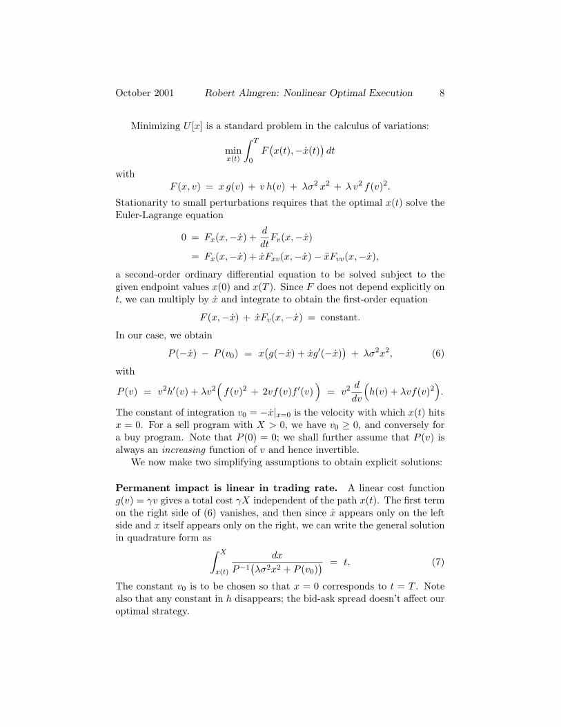
Minimizing U [x] is a standard problem in the calculus of variations:
minx(t)
∫ T
0F
(x(t),−x(t)
)dt
withF (x, v) = x g(v) + v h(v) + λσ2 x2 + λ v2 f(v)2.
Stationarity to small perturbations requires that the optimal x(t) solve theEuler-Lagrange equation
0 = Fx(x,−x) +d
dtFv(x,−x)
= Fx(x,−x) + xFxv(x,−x)− xFvv(x,−x),
a second-order ordinary differential equation to be solved subject to thegiven endpoint values x(0) and x(T ). Since F does not depend explicitly ont, we can multiply by x and integrate to obtain the first-order equation
F (x,−x) + xFv(x,−x) = constant.
In our case, we obtain
P (−x) − P (v0) = x(g(−x) + xg′(−x)
)+ λσ2x2, (6)
with
P (v) = v2h′(v) + λv2(
f(v)2 + 2vf(v)f ′(v))
= v2 d
dv
(h(v) + λvf(v)2
).
The constant of integration v0 = −x|x=0 is the velocity with which x(t) hitsx = 0. For a sell program with X > 0, we have v0 ≥ 0, and conversely fora buy program. Note that P (0) = 0; we shall further assume that P (v) isalways an increasing function of v and hence invertible.
We now make two simplifying assumptions to obtain explicit solutions:
Permanent impact is linear in trading rate. A linear cost functiong(v) = γv gives a total cost γX independent of the path x(t). The first termon the right side of (6) vanishes, and then since x appears only on the leftside and x itself appears only on the right, we can write the general solutionin quadrature form as
∫ X
x(t)
dx
P−1(λσ2x2 + P (v0)
) = t. (7)
The constant v0 is to be chosen so that x = 0 corresponds to t = T . Notealso that any constant in h disappears; the bid-ask spread doesn’t affect ouroptimal strategy.

October 2001 Robert Almgren: Nonlinear Optimal Execution 9
The imposed time horizon is infinite. Since P (·) is an increasing func-tion, so is P−1(·). It is thus clear that as v0 decreases towards zero, theliquidation time T increases. If no time horizon is exogeneously imposed,then we obtain the longest possible liquidation time by setting v0 = 0, whichleads to the quadrature problem
∫ X
x(t)
dx
P−1(λσ2x2)= t.
We can often find analytic solutions to this problem when (7) with v0 6= 0would be too intractable. These solutions will still give nearly completeliquidation in a finite time determined by market parameters.
3 Nonlinear cost functions
Restricting our attention to a sell program, with v ≥ 0, we take the tempo-rary impact functions
h(v) = η vk f(v) = 0.
with k > 0 (for a buy program we would change signs in an obvious way).The linear case corresponds to k = 1. As noted above, we have neglected apossible constant in h corresponding to the bid-ask spread. Then
P (v) = ηk vk+1
which, for the general case of a finite time horizon with v0 ≥ 0, leads to thequadrature problem
∫ X
x(t)
(λσ2
kηx2 + v k+1
0
)− 1k+1
dx = t.
Taking v0 = 0, we can solve explicitly for the longest optimal trajectories:
x(t)X
=
(1 +
1− k
1 + k
t
T∗
)−(1+k)/(1−k)
if 0 < k < 1,
exp(− t
T∗
)if k = 1,
(1− k − 1
k + 1t
T∗
)(k+1)/(k−1)
if k > 1.
(8)
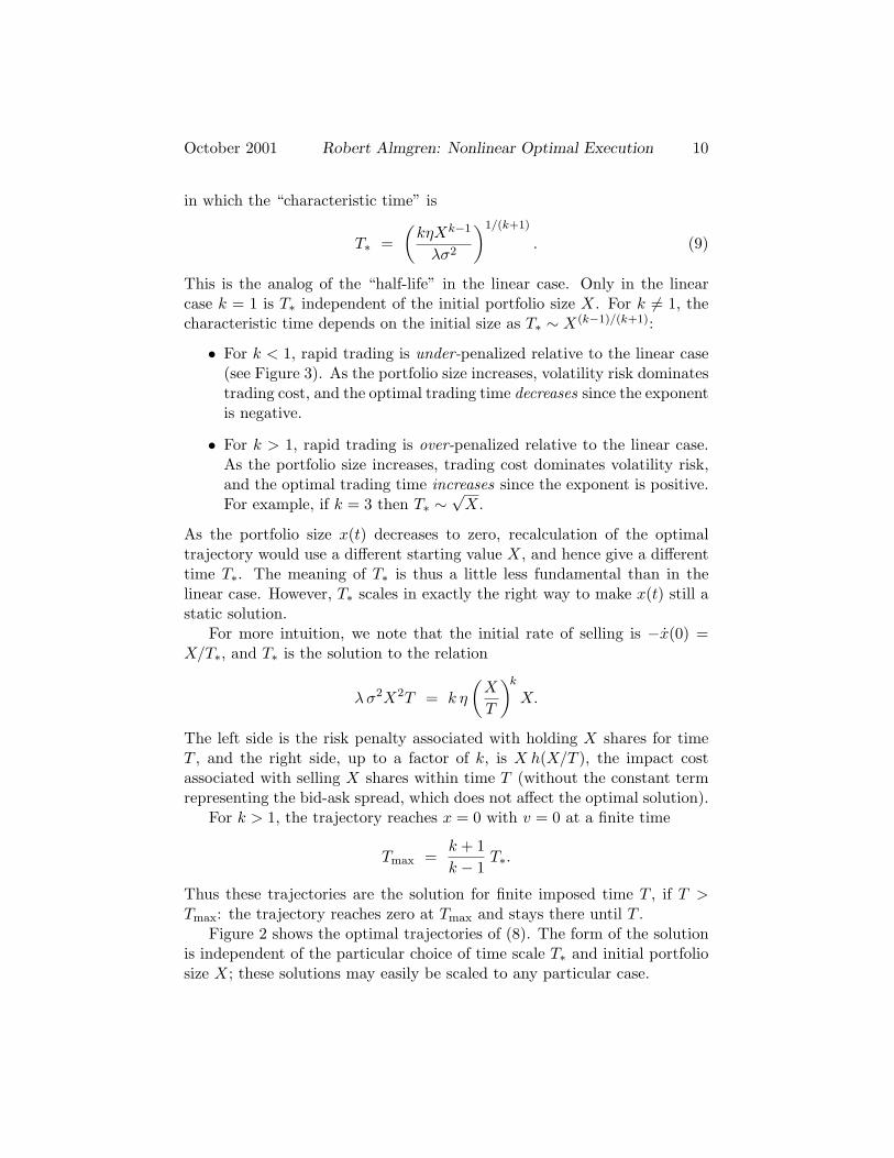
October 2001 Robert Almgren: Nonlinear Optimal Execution 10
in which the “characteristic time” is
T∗ =(
kηXk−1
λσ2
)1/(k+1)
. (9)
This is the analog of the “half-life” in the linear case. Only in the linearcase k = 1 is T∗ independent of the initial portfolio size X. For k 6= 1, thecharacteristic time depends on the initial size as T∗ ∼ X(k−1)/(k+1):
• For k < 1, rapid trading is under-penalized relative to the linear case(see Figure 3). As the portfolio size increases, volatility risk dominatestrading cost, and the optimal trading time decreases since the exponentis negative.
• For k > 1, rapid trading is over-penalized relative to the linear case.As the portfolio size increases, trading cost dominates volatility risk,and the optimal trading time increases since the exponent is positive.For example, if k = 3 then T∗ ∼
√X.
As the portfolio size x(t) decreases to zero, recalculation of the optimaltrajectory would use a different starting value X, and hence give a differenttime T∗. The meaning of T∗ is thus a little less fundamental than in thelinear case. However, T∗ scales in exactly the right way to make x(t) still astatic solution.
For more intuition, we note that the initial rate of selling is −x(0) =X/T∗, and T∗ is the solution to the relation
λσ2X2T = k η
(X
T
)k
X.
The left side is the risk penalty associated with holding X shares for timeT , and the right side, up to a factor of k, is X h(X/T ), the impact costassociated with selling X shares within time T (without the constant termrepresenting the bid-ask spread, which does not affect the optimal solution).
For k > 1, the trajectory reaches x = 0 with v = 0 at a finite time
Tmax =k + 1k − 1
T∗.
Thus these trajectories are the solution for finite imposed time T , if T >Tmax: the trajectory reaches zero at Tmax and stays there until T .
Figure 2 shows the optimal trajectories of (8). The form of the solutionis independent of the particular choice of time scale T∗ and initial portfoliosize X; these solutions may easily be scaled to any particular case.

October 2001 Robert Almgren: Nonlinear Optimal Execution 11
0 1 2 3 4 50
10%
20%
30%
40%
50%
60%
70%
80%
90%
1
k = 2
k = 0.5
Time t (in units of T*)
Sha
res
x(t)
(as
frac
tion
of in
itial
X)
Figure 2: Optimal solution trajectories x(t), for k = 12 , 1, 2. For each value
of k, the solution has a “universal” form, which may be scaled as necessaryfor different choice of time scales T∗ and initial portfolio size X. The diskshows Tmax = 3T∗ for k = 2.
October 2001 Robert Almgren: Nonlinear Optimal Execution 12
A sense of the differences between these solutions may be gained bynoting that for short times, all the optimal trajectories are fairly close toeach other; but the “tail” of the trajectory is extended for small values of k,which strongly penalize trading at slow rates. For example, at t = T∗, theoptimal trajectories reduce the holdings to 30%, 37%, and 42% of the initialportfolio, for k = 2, 1, 1
2 respectively. At t/T∗ = 3, the trajectory for k = 2has reached x = 0 and remains there, the trajectory for k = 1 retains 5% ofits initial holdings, and the trajectory for k = 2 retains 12.5% of the initial.The relative differences become even more pronounced as time continues.
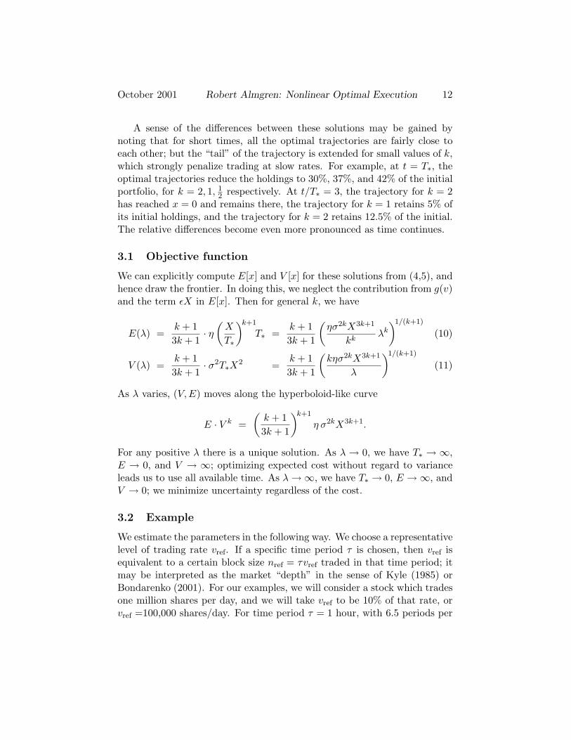
3.1 Objective function
We can explicitly compute E[x] and V [x] for these solutions from (4,5), andhence draw the frontier. In doing this, we neglect the contribution from g(v)and the term εX in E[x]. Then for general k, we have
E(λ) =k + 13k + 1
· η(
X
T∗
)k+1
T∗ =k + 13k + 1
(ησ2kX3k+1
kkλk
)1/(k+1)
(10)
V (λ) =k + 13k + 1
· σ2T∗X2 =k + 13k + 1
(kησ2kX3k+1
λ
)1/(k+1)
(11)
As λ varies, (V,E) moves along the hyperboloid-like curve
E · V k =(
k + 13k + 1
)k+1
η σ2kX3k+1.
For any positive λ there is a unique solution. As λ → 0, we have T∗ → ∞,E → 0, and V → ∞; optimizing expected cost without regard to varianceleads us to use all available time. As λ →∞, we have T∗ → 0, E →∞, andV → 0; we minimize uncertainty regardless of the cost.
3.2 Example
We estimate the parameters in the following way. We choose a representativelevel of trading rate vref. If a specific time period τ is chosen, then vref isequivalent to a certain block size nref = τvref traded in that time period; itmay be interpreted as the market “depth” in the sense of Kyle (1985) orBondarenko (2001). For our examples, we will consider a stock which tradesone million shares per day, and we will take vref to be 10% of that rate, orvref =100,000 shares/day. For time period τ = 1 hour, with 6.5 periods per

October 2001 Robert Almgren: Nonlinear Optimal Execution 13
day, this rate is equivalent to trading a block of approximately 15,300 sharesin each hour.
Next, we choose the price impact href which would be incurred by steadytrading at the reference rate vref. In our example, we shall assume the shareprice is $50/share, and we assume that trading vref =100,000 shares/dayincurs a price impact of 1%, or $0.50 /share.
Finally, we choose a value for the exponent k which best fits our beliefabout how the price impact would depend on trading rate for rates largeror smaller than vref. The choice k = 1 corresponds to linear dependence ofprice impact on rate; k > 1 means that large trading rates or block sizeshave a disproportionately large effect on price, while k < 1 means that largetrading rates or block sizes have a relatively smaller impact.
The impact model is then written
h(v) = href
(v
vref
)k
, or η =href
v kref
. (12)
Figure 3 illustrates this model.We also suppose that our stock has annual volatility of 32%, for expected
daily price changes of σ = $1/share · √day. We shall consider a portfolioof initial size X = 100, 000, equal to one-tenth of the daily volume. Wehave then specified enough information to construct the efficient frontier(10,11) from
(E(λ), V (λ)
)for any chosen k, describing the family of optimal
solutions as the risk-aversion parameter λ ranges over all possible values0 < λ < ∞. To construct particular optimal solutions, we need to specify avalue for λ.
The results are shown numerically in Table 1. For any value of k, thenatural liquidation time T∗ increases with the “risk-tolerance” parameter1/λ; as both increase, the expected cost decreases and the variance increases.
The dependence on exponent k, for fixed href and vref, is shown in Fig-ure 4. For large values of λ, the optimal trajectories all execute rapidly, toreduce the volatility risk associated with holding the portfolio. When thetrading rate is larger than vref, costs increase with increasing k, so larger kleads to slightly slower trading.
Conversely, for small λ, trading generally proceeds more slowly thanvref in order to minimize total expected cost. In this regime, smaller k ismore expensive, and leads to relatively slower trading. In the intermediateparameter regime, the trajectories cross over from one behavior to the other:larger k suggests slower trading at the beginning when the rate is large, thenrelatively more rapid trading in the tail.

October 2001 Robert Almgren: Nonlinear Optimal Execution 14
0 0.5 1 1.5 2
x 105
0
0.1
0.2
0.3
0.4
0.5
0.6
0.7
0.8
0.9
1
k = 0.5
k = 1
k = 2
v = vref
h = href
Trading rate v (shares/day)
Pric
e im
pact
h(v
) ($
/sha
re)
Figure 3: Nonlinear temporary impact model h(v). A representative tradingrate vref and a representative price impact href are chosen, and these valuesare extended to general v using an exponent k.

October 2001 Robert Almgren: Nonlinear Optimal Execution 15
Note that we may rewrite (9) as
T∗ =(
khref
λσ2X
)1/(k+1) (X
vref
)k/(k+1)
from which it is clear that T∗ → X/vref as k →∞, regardless of the values ofthe other parameters. In this limit, trading more rapidly than the referencerate is very strongly penalized, while trading more slowly is almost withoutcost, so the optimal strategy is always to trade exactly at the critical rate.
Finally, since λ is a difficult parameter to select in practice, let us notethat it may be estimated if a time scale T∗ is chosen: from (9,12) we find
λ = k ·href
(X/T∗vref
)k
·Xσ2T∗X2
.
The numerator is the price concession per share for trading at a constant rateX/T∗, multiplied by the total number of shares X to get total expected cost;the denominator is the variance that would be incurred by holding X sharesfor time T∗. We multiply this ratio by k to correct for the nonlinearitieswhich are ignored in this simple description.
4 Trading-enhanced risk
Now we take (for a sell program with v ≥ 0)
h(v) = η v, f(v) = α + β v.
The deterministic part of the temporary impact is the linear case k = 1 ofthe previous section.
The constant term in f(v), with coefficient α, represents a constantuncertainty in the realized sale price, independent of our rate of selling andof the underlying price process. We minimize the total risk associated withthis term by splitting our sale into as many equal parts as possible; thus thisterm pushes us toward the linear trajectory. The linear term, with coefficientβ, represents the increase in variance caused by nonzero amounts of selling.This term even more strongly pushes us toward the linear trajectory.
Then (with x = −v ≤ 0) the ODE (6) has
P (v) =(η + λα2
)v2 + 4λαβ v3 + 3λβ2 v4.

October 2001 Robert Almgren: Nonlinear Optimal Execution 16
k = 12 k = 1 k = 2
1/λ = 1 0.02 0.07 0.22
10 0.09 0.22 0.46
T∗ 100 0.40 0.71 1.00
1,000 1.84 2.24 2.15
10,000 8.55 7.07 4.64
1/λ = 1 221 354 462
10 103 112 99
E 100 48 35 21
1,000 22 11 5
10,000 10 4 1
1/λ = 1 11 19 30
10 23 33 45√
V 100 49 59 65
1,000 105 106 96
10,000 226 188 141
Table 1: Optimal time scale T∗, expected cost E, and standard deviation ofcost
√V , as functions of risk-tolerance parameter 1/λ and temporary impact
exponent k. Market and portfolio parameters are as given in the text (initialportfolio value is $5 million). As k is varied, the reference values href andvref are held constant; thus the coefficient η varies as in (12). Time T∗ ismeasured in days; 1/λ, E, and
√V are in thousands of dollars.

October 2001 Robert Almgren: Nonlinear Optimal Execution 17
0 0.5 1 1.50
20
40
60
80
100
k = 2
k = 0.5
1/λ = 10
Time (days)
Tho
usan
ds o
f sha
res
0 1 2 3 4 50
20
40
60
80
100
k = 2
k = 0.5
1/λ = 200
Time (days)
Tho
usan
ds o
f sha
res
0 5 100
20
40
60
80
100
k = 2
k = 0.5
1/λ = 2000
Time (days)
Tho
usan
ds o
f sha
res
Figure 4: Optimal trajectories for different values of parameters as shownin Table 1 and in the text. For each value of the risk-tolerance parameter1/λ, we vary the exponent k for fixed values of href and vref. The directionin which the time scale changes with k depends on the value of 1/λ.

October 2001 Robert Almgren: Nonlinear Optimal Execution 18
The polynomial P (v) has P (0) = 0 and is increasing for v ≥ 0, so the graphof the trajectory is always convex, and the inverse function P−1 is welldefined. (For a buy program, with x ≥ 0, the sign of the odd term in P (v)is reversed.) Since P (v) ∼ O(v2) for v near zero, the integrand appearingin the quadrature formulation (7) behaves like O(x−1) as x → 0 for v0 = 0,and there is no “hard” maximum time as we found above for k > 1.
4.1 Constant enhanced risk
To obtain analytical solutions, we consider two special cases. The first is β =0; with this assumption, the price uncertainty on each trade is independentof the size of the trade. We then find the solution for v0 = 0
x(t) = X exp(− t
T∗
), T∗ =
√η + λα2
λσ2.
This is a pure exponential solution, except that the time constant has beenincreased by adding the additional variance per transaction to the impactcoefficient: η 7→ η + λα2. The value functions are
E(λ) =12η
X2
T∗=
12X2
√λη2σ2
η + λα2
V (λ) =12X2σ2T∗
(1 +
α2
σ2T 2∗
)=
12X2 σ√
λ· η + 2λα2
√η + λα2
.
The optimal value functions change in a more complicated way than thetrajectory. As λ → 0 we find the same behavior as in Section 3.1: E → 0and V →∞, since we do not care about the enhanced risk. In contrast, asλ → ∞, all quantities have finite limits: T∗ → α/σ, E → 1
2ηX2/T∗, andV → ασX2. Since trading itself introduces variance, risk-aversion and costreduction both encourage you to spread the trading over several periods; theminimum-variance solution takes finite time and has finite cost.
4.2 Linear enhanced risk
Also, let us consider the special case α = 0, so that P (v) = ηv2 + 3λβ2v4,and we readily find
P−1(w) =
√√η2 + 12λβ2w − η
6λβ2.
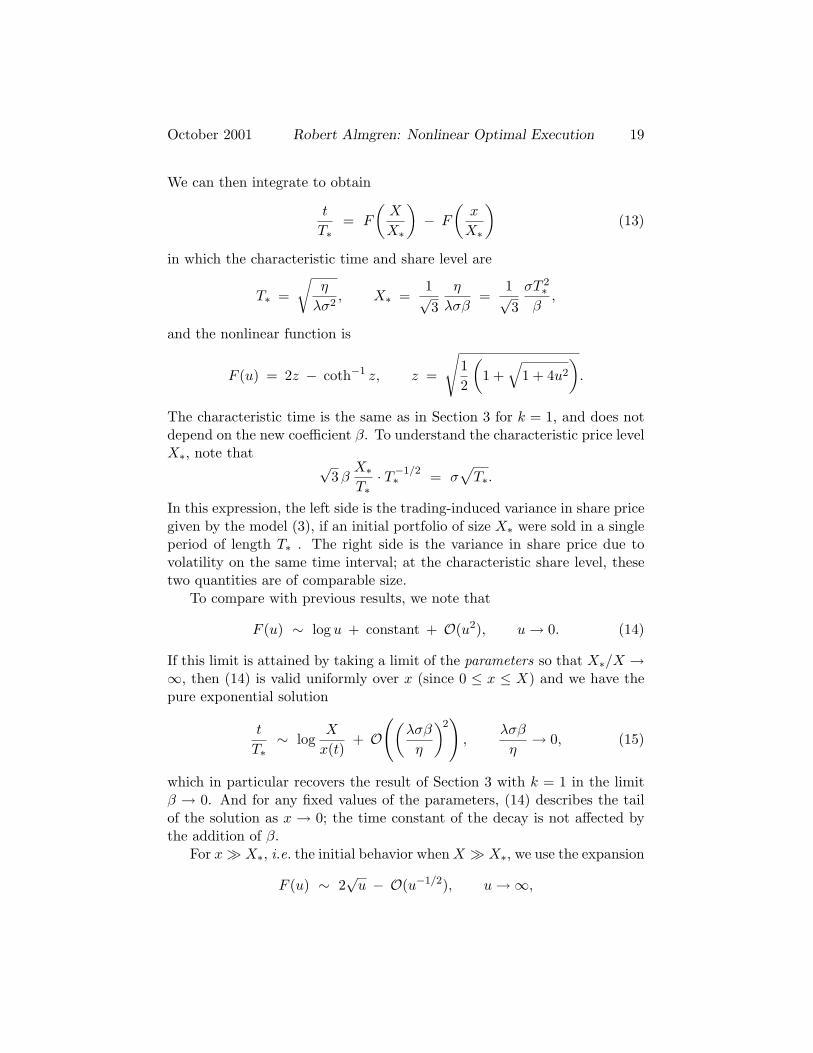
October 2001 Robert Almgren: Nonlinear Optimal Execution 19
We can then integrate to obtain
t
T∗= F
(X
X∗
)− F
(x
X∗
)(13)
in which the characteristic time and share level are
T∗ =√
η
λσ2, X∗ =
1√3
η
λσβ=
1√3
σT 2∗β
,
and the nonlinear function is
F (u) = 2z − coth−1 z, z =
√12
(1 +
√1 + 4u2
).
The characteristic time is the same as in Section 3 for k = 1, and does notdepend on the new coefficient β. To understand the characteristic price levelX∗, note that √
3βX∗T∗
· T−1/2∗ = σ
√T∗.
In this expression, the left side is the trading-induced variance in share pricegiven by the model (3), if an initial portfolio of size X∗ were sold in a singleperiod of length T∗ . The right side is the variance in share price due tovolatility on the same time interval; at the characteristic share level, thesetwo quantities are of comparable size.
To compare with previous results, we note that
F (u) ∼ log u + constant + O(u2), u → 0. (14)
If this limit is attained by taking a limit of the parameters so that X∗/X →∞, then (14) is valid uniformly over x (since 0 ≤ x ≤ X) and we have thepure exponential solution
t
T∗∼ log
X
x(t)+ O
((λσβ
η
)2)
,λσβ
η→ 0, (15)
which in particular recovers the result of Section 3 with k = 1 in the limitβ → 0. And for any fixed values of the parameters, (14) describes the tailof the solution as x → 0; the time constant of the decay is not affected bythe addition of β.
For x À X∗, i.e. the initial behavior when X À X∗, we use the expansion
F (u) ∼ 2√
u − O(u−1/2), u →∞,
October 2001 Robert Almgren: Nonlinear Optimal Execution 20
which gives
x(t) ∼ X∗
(C − 1
2t
T∗
)2
, x À X∗, (16)
with C = 12F (1). This is the same solution constructed in Section 3 for
k = 3, with η = λβ2.The solution (13), together with the asymptotic expressions (15,16) are
shown in Figure 5.Thus the optimal strategy is as follows. Assuming X > X∗, trade ini-
tially using the trajectories of Section 3 with k = 3 and η = λβ2. Thatis, volatility due to trading completely dominates the intrinsic volatility σ.As x(t) reaches the level X∗, switch to the optimal solution in the linearcase k = 1, with other parameters taking their market values. In the tail,trading-enhanced risk is a negligible effect compared to volatility.
4.3 Example
We focus on the case in the previous section, in which α = 0 and β 6= 0 sothat trading-enhanced risk increases linearly with block size with no constantterm. To estimate the coefficients, we must return to our discrete-timemodel. With h(v) = ηv and f(v) = βv, the price model (3) becomes
Sk = Sk−1 − η nk τ−1 + β nk τ−3/2 ξk.
Let us assume that for a particular choice of the trading interval τ , thestandard deviation of price concession associated with trading-enhanced riskis a fraction ρ of the deterministic impact, since both of these quantities arelinearly proportional to the block size. That is, we assume
β nk τ−3/2 = ρ · η nk τ−1
orβ = ρ τ1/2η
which gives
X∗ =1√3 ρ
· 1λστ1/2
.
At this portfolio size, the volatility risk of holding the portfolio roughlybalances the trading-induced risk of selling along the optimal trajectory.Although both of these quantities are risks, the expression for X∗ involvesλ through its influence on the trading time T∗.

October 2001 Robert Almgren: Nonlinear Optimal Execution 21
−4 −2 0 2 40
1
2
3
4
5
6
7
8
t/T* (arbitrary origin)
x/X
*
Large x
Small x
Figure 5: The universal optimal trajectory for linear trading-enhanced risk,scaled by the characteristic time T∗ and share level X∗, together with itsasymptotic behavior for large and small x. The solution for any desiredparameters may be constructed by scaling this picture and choosing an ap-propriate time origin. When x is large compared with X∗, the solution isessentially the nonlinear solution of Section 3 with exponent k = 3; this hap-pens for the initial phase of trading if X is large compared with X∗. Whenx is small compared with X∗, the solution is essentially the linear solutionof Section 3 with k = 1; this applies to the tail of the trajectory for any X,or to the entire trading trajectory if X is smaller than X∗.

October 2001 Robert Almgren: Nonlinear Optimal Execution 22
Let us take market parameters as in Section 3.2, with 1/λ =$10,000,corresponding to the first panel of Figure 4 with liquidation in less than oneday. Let us divide trading into one-hour time intervals, so τ = (2/13) day,and let us take ρ = 1/2. We then obtain β = 10−6 $ · day3/2/share2, andX∗ = 30,000 shares corresponding to a portfolio size of $1.5M. A liquidationproblem with initial value greater than this will begin in the large-x regimewhere trading-enhanced risk is dominant, and end in the small-x regimewhere it is negligible.
5 Conclusions
We have obtained explicit analytical solutions for certain special cases ofthe impact model. First, we neglected the effect of trading-enhanced risk,and took the impact function to be a simple power law. The solutions inthis case are a straightforward nonlinear extension of the results in Almgrenand Chriss (2000); the exponential solutions obtained there are a particulardividing case of these power-law solutions.
With trading-enhanced risk, we considered two particular cases with lin-ear impact functions. If the price uncertainty per transaction is independentof transaction size, then the optimal trajectories are given by the previousresults, simply augmenting the impact coefficient by the additional vari-ance. A risk-averse trader lengthens his trade program, diversifying awaysome variance by spreading the execution over more different transactionsat the expense of slightly higher volatility risk.
If the price uncertainty per transaction is linearly proportional to trans-action size, then a characteristic portfolio size emerges, above which reduc-tion of this added variance is the dominant effect. In this regime, tradetrajectories are equivalent to the previous power-law solutions with expo-nent equal to three. For portfolios smaller than this size, the new effect maybe neglected relative to deterministic impact costs and ordinary volatility.
Throughout this paper, we have focused on obtaining explicit solutionsfor the sake of analytical insight. Numerical solution would be quite straight-forward, and would allow lifting the restrictions described above and theconsideration of a more general class of models.
Portfolios of multiple assets are an interesting extension. Already in thelinear case (Almgren and Chriss 2000), to obtain explicit solutions it is nec-essary to make simplifying assumptions about cross-impacts, for example,that trading in each asset affects only the price of that asset. Even withthat assumption, the nonlinear formulation opens a wide class of possible
October 2001 Robert Almgren: Nonlinear Optimal Execution 23
models: for example, should the exponent be the same for each asset? De-termination and characterization of the optimal trajectories in this case is atopic for future work.
References
Almgren, R. and N. Chriss (1999). Value under liquidation. Risk 12 (12), 61–63.Almgren, R. and N. Chriss (2000). Optimal execution of portfolio transactions.
J. Risk 3 (2), 5–39.Artzner, P., F. Delbaen, J.-M. Eber, and D. Heath (1999). Coherent measures of
risk. Math. Finance 9, 203–228.Barra (1997). Market Impact Model Handbook.Basak, S. and A. Shapiro (2001). Value-at-Risk-based risk management: Optimal
policies and asset prices. Rev. Financial Studies 14, 371–405.Bessembinder, H. and H. M. Kaufman (1997). A comparison of trade execution
costs for NYSE and NASDAQ-listed stocks. J. Fin. Quant. Anal. 32, 287–310.
Bondarenko, O. (2001). Competing market makers, liquidity provision, and bid-ask spreads. J. Financial Markets 4 (3), 269–308.
Chakravarty, S. (2001). Steath-trading: Which traders’ trades move prices? J.Financial Econ. 61, 289–307.
Chan, L. K. C. and J. Lakonishok (1993). Institutional trades and intraday stockprice behavior. J. Financial Econ. 33, 173–199.
Chan, L. K. C. and J. Lakonishok (1995). The behavior of stock prices aroundinstitutional trades. J. Finance 50, 1147–1174.
Chordia, T., A. Subrahmanyam, and V. R. Anshuman (2001). Trading activityand expected stock returns. J. Financial Econ. 59, 3–32.
Grinold, R. C. and R. N. Kahn (1999). Active Portfolio Management (2nd ed.),Chapter 16, pp. 473–475. McGraw-Hill.
Hasbrouck, J. and R. A. Schwartz (1988). Liquidity and execution costs in equitymarkets. J. Portfolio Management 14 (Spring), 10–16.
Hasbrouck, J. and D. J. Seppi (2001). Common factors in prices, order flows,and liquidity. J. Financial Econ. 59, 383–411.
Holthausen, R. W., R. W. Leftwich, and D. Mayers (1987). The effect of largeblock transactions on security prices: A cross-sectional analysis. J. FinancialEcon. 19, 237–267.
Holthausen, R. W., R. W. Leftwich, and D. Mayers (1990). Large-block trans-actions, the speed of response, and temporary and permanent stock-priceeffects. J. Financial Econ. 26, 71–95.

October 2001 Robert Almgren: Nonlinear Optimal Execution 24
Huang, R. D. and H. R. Stoll (1997). The components of the bid-ask spread: Ageneral approach. Rev. Financial Studies 10 (4), 995–1034.
Huberman, G. and W. Stanzl (2001). Optimal liquidity trading. Preprint.Jones, C. M. and M. L. Lipson (1999). Execution costs of institutional equity
orders. J. Financial Intermediation 8, 123–140.Kahn, R. N. (1993). How the execution of trades is best operationalized. In
K. F. Sherrerd (Ed.), Execution Techniques, True Trading Costs, and theMicrostructure of Markets. AIMR.
Keim, D. B. and A. Madhavan (1995). Anatomy of the trading process: Empiricalevidence on the behavior of institutional traders. J. Financial Econ. 37, 371–398.
Keim, D. B. and A. Madhavan (1997). Transactions costs and investmentstyle: An inter-exchange analysis of institutional equity trades. J. Finan-cial Econ. 46, 265–292.
Konishi, H. and N. Makimoto (2001). Optimal slice of a block trade. Preprint.Koski, J. L. and R. Michaely (2000). Prices, liquidity, and the information content
of trades. Rev. Financial Studies 13, 659–696.Kraus, A. and H. R. Stoll (1972). Price impacts of block trading on the New
York Stock Exchange. J. Finance 27, 569–588.Kyle, A. S. (1985). Continuous auctions and insider trading. Econometrica 53,
1315–1336.Loeb, T. F. (1983). Trading costs: The critical link between investment informa-
tion and results. Financial Analysts Journal 39, 39–44.Perold, A. F. (1988). The implementation shortfall: Paper versus reality. J. Port-
folio Management 14 (Spring), 4–9.Perold, A. F. and R. S. Salomon, Jr. (1991). The right amount of assets under
management. Financial Analysts J. 47 (May-June), 31–39.Rickard, J. T. and N. G. Torre (1999). Information systems for optimal transac-
tion implementation. J. Management Information Systems 16, 47–62.Stoll, H. R. (1989). Inferring the components of the bid-ask spread: Theory and
empirical tests. J. Finance 44, 115–134.Wagner, W. H. and M. Banks (1992). Increasing portfolio effectiveness via trans-
action cost management. J. Portfolio Management 19, 6–11.