optimal fiscal and monetary policy

Optimal Fiscal and Monetary Policy

1

Background

• We Have Discussed the Construction and Estimation of DSGE Models• Next, We Turn to Analysis• Most Basic Policy Question:

– How Should the Policy Variables of the Government be Set?– What is Optimal Policy? What Should R Be, How Volatile Should P Be?

• In Past 10 Years, Profession Has Explored Operating Characteristics of SimplePolicy Rules– One Finding: A Taylor Rule with High Weight on Inflation Works Well in

New-Keynesian Models• Recent Development:

– Increasingly, Analysts Studying Optimal Policy– Perhaps Because there is a Perception that Current DSGE Models Fit Data

Well• We Will Review Some of this Work.

10

Modern Quantitative Analysis of Optimal Policy

• Case Where Intertemporal Government Budget Constraint Does Not Bind

– Example - Current Generation of Monetary Models∗ Assume Presence of Lump-Sum Taxes Used to Ensure Government

Budget Constraint is Satisfied

– Optimal Policy Studied, Among Others, By Schmitt-Grohe and Uribe(2004), Levin, Onatski, Williams, Williams (2005), and References TheyCite.

• Case Where Intertemporal Government Budget Constraint Binds

– Example - When the Government Does not Have Access to Distorting Taxes– Chari-Christiano-Kehoe (1991, 1994), Schmitt-Grohe and Uribe (2001),

Siu (2001), Benigno-Woodford (2003, 2005), Others.

13

Outline

• Optimal Monetary and Fiscal Policy When the Intertemporal Budget ConstraintBinds

– Analyze the Friedman-Phelps Debate over the Optimal Nominal Rate ofInterest.

– What is the Optimal Degree of Price Variability?– How Should Policy React to a Sudden Jump in G?– Log-Linearization as a Solution Strategy– Woodford’s Timeless Perspective

• Optimal Monetary Policy When the Intertemporal Budget Constraint Can beIgnored.

– Log-Linearization as a Solution Strategy

14

Optimal Policy in the Presence of a BudgetConstraint

• Sketch of Phelps-Friedman Debate

• Some Ideas from Public Finance - Primal Problem

• Simple One-Period Example

• Determining Who is Right, Friedman or Phelps, Using Lucas-Stokey Cash-Credit Good Model

• Financing a Sudden Expenditure (Natural Disaster): Barro versus Ramsey.

15

Friedman-Phelps Debate

• Money Demand:M

P= exp[−αR]

• Friedman:

a. Efforts to Economize Cash Balances when R High are Socially Wasteful

b. Set R as Low As Possible: R = 1.

c. Since R = 1 + r + π, Friedman Recommends π = −r.

i. r ∼ exogenous (net) real interest rate rateii. π ∼ inflation rate, π = (P − P−1)/P−1

16

Friedman-Phelps Debate ...

• Phelps:a. Inflation Acts Like a Tax on Cash Balances -

Seigniorage =Mt −Mt−1

Pt=Mt

Pt− Pt−1

Pt

Mt−1Pt−1

≈ M

P

π

1 + π

b. Use of Inflation Tax Permits Reducing Some Other Tax Rate

c. Extra Distortion in Economizing Cash Balances Compensated by ReducedDistortion Elsewhere.

d. With Distortions a Convex Function of Tax Rates, Would Always Want toTax All Goods (Including Money) At Least A Little.

e. Inflation Tax Particularly Attractive if Interest Elasticity of Money DemandLow.

17

Question: Who is Right, Friedman or Phelps?

• Answer: Friedman Right Surprisingly Often

• Depends on Income Elasticity of Demand for Money

• Will Address the Issue From a Straight Public Finance Perspective, In theSpirit of Phelps.

• Easy to Develop an Answer, Exploiting a Basic Insight From Public Finance.

18

Question: Who is Right, Friedman or Phelps? ...

Some Basic Ideas from Ramsey Theory• Policy, π, Belonging to the Set of ‘Budget Feasible’ Policies, A.• Private Sector Equilibrium Allocations, Equilibrium Allocations, x,

Associated with a Given π; x ∈ B.

• Private Sector Allocation Rule, mapping from π to x (i.e., π : A→ B).• Ramsey Problem: Maximize, w.r.t. π, U(x(π)).• Ramsey Equilibrium: π∗ ∈ A and x∗, such that π∗ solves Ramsey Problem

and x∗ = x(π∗). ‘Best Private Sector Equilibrium’.• Ramsey Allocation Problem: Solve, x = argmax U(x) for x ∈ B

• Alternative Strategy for Solving the Ramsey Problem:a. Solve Ramsey Allocation Problem, to Find x.b. Execute the Inverse Mapping, π = x−1(x).

c. π and x Represent a Ramsey Equilibrium.

• Implementability Constraint: Equations that Summarize Restrictions onAchievable Allocations, B, Due to Distortionary Tax System.

19

Question: Who is Right, Friedman or Phelps? ...

Policy, π

Set, A, of Budget-Feasible Policies

Private sector Allocation Rule, x(π)

Set, B, of Private Sector Allocations Achievable by Some Budget-Feasible Policy

Private Sector Equilibrium

Allocations, x

Utility

20

Example

• Households:

maxc,l

u(c, l)

c ≤ z(1− τ )l,

z ∼ wage rate

τ ∼ labor tax rate

21

Example ...

• Household Problem Implies Private Sector Allocation Rules, l(τ ), c(τ ),defined by:

ucz(1− l) + ul = 0, c = (1− τ )zl

l(τ) l

u[z(1-τ)l,l] ucz(1-τ)+ul=0

Private Sector Allocation Rules: l(τ), c(τ) = z(1-τ)l

22

Example ...

• Ramsey Problem:

maxτ

u(c(τ ), l(τ ))

subject to g ≤ zl(τ )τ

• Ramsey Equilibrium: τ ∗, c∗, l∗ such that

a. c∗ = c(τ ∗), l∗ = l(τ ∗)

∗ ‘Private Sector Allocations are a Private Sector Equilibrium’

b. τ ∗ Solves Ramsey Problem

∗ ‘Best Private Sector Equilibrium’

23

Analysis of Ramsey Equilibrium

• Simple Utility Specification:

u(c, l) = c− 12l2

• Two Ways to Compute the Ramsey Equilibrium

a. Direct Way: Solve Ramsey Problem (In Practice, Hard)

b. Indirect Way: Solve Ramsey Allocation Problem, or Primal Problem (CanBe Easy)

24

Analysis of Ramsey Equilibrium ...

Direct Approach• Private Sector Allocation Rules:

c(τ ) = z2(1− τ )2, l(τ ) = z(1− τ )

• ‘Utility Function’ for Ramsey Problem:

u(c(τ ), l(τ )) =1

2z2(1− τ )2

• Constraint on Ramsey Problem:g ≤ zl(τ )τ = z2(1− τ )τ

• Ramsey Problem:maxτ

1

2z2(1− τ )2

subject to : g ≤ τz2(1− τ ).

34


¼z2

g

τz2(1-τ) ‘Laffer Curve’

0 1 τ

½z2(1-τ)2

τ1 τ2

τ* = τ1 =½ -½[ 1 – 4 g/z2 ]½ τ2 =½+½[ 1 – 4 g/z2 ]½

l(τ*) =½{ z+[ z2 – 4 g ]½ }

A

Government Preferences

35


Indirect Approach• Approach: Solve Ramsey Allocation Problem, Then ‘Inverse Map’ Back into

Policies• Problem: Would Like a Characterization of B that Only Has (c, l), Not the

PoliciesB = {c, l : ∃τ , with ucz(1− τ ) + ul = 0,

c = (1− τ )zl, g ≤ τzl}• Solution: Rearrange Equations in B, So That Only (c, l) Appears

(∗) ucc + ull = 0, (∗∗) c + g ≤ zl.

• Conclude: B = D, where:

D =

⎧⎪⎪⎨⎪⎪⎩(c, l) : c + g ≤ zl| {z }resource constraint

, ucc + ull = 0| {z }implementability constraint

⎫⎪⎪⎬⎪⎪⎭

43


• Express Ramsey Allocation Problem:

maxc,l

u(c, l), subject to (c, l) ∈ D

• Alternatively:

maxc,l

u(c, l),

s.t. ucc + ull = 0, c + g ≤ zl

• Or,

maxl

1

2l2

s.t. l2 + g ≤ zl

46


0

Ramsey Allocation Problem:

Max ½l2 Subject to l2 + g ≤ zl Solution: l2 = ½{ z + [ z2 - 4g ]½ } Same Result as Before!

l2 - zl +g = 0

½z l1 l2

g - ¼z2

½l2

47


Lucas-Stokey Cash-Credit Good Model• Households• Firms• Government

48


Households• Household Preferences:

∞Xt=0

βtu(c1t, c2t, lt),

c1t ˜ cash goods, c2t ˜ credit goods, lt ˜ labor

• Distinction Between Cash and Credit Goods:

– All Goods Paid With Cash At the Same Time, After Goods Market, in AssetMarket

– Cash Good: Must Carry Cash In Pocket Before Consuming It

Mt ≥ Ptc1t

– Credit Good: No Need to Carry Cash Before Purchase.

49


Household Participation in Asset and Good Markets

• Asset Market: First Half of Period, When Household Settles Financial ClaimsArising From Activities in Previous Asset Market and in Previous GoodsMarket.

• Goods Market: Second Half of Period, Goods are Consumed, Labor Effort isApplied, Production Occurs.

50


t t+1

Asset Market Goods Market

Sources of Cash for Household: • Md

t-1 - Pt-1c1,t-1 - Pt-1c2,t-1 • Rt-1Bd

t-1 • (1-τt-1)zlt-1

Uses of Cash • Bonds, Bd

t • Cash, Md

t

• c1,t , c2,t Purchased • lt Supplied • Production Occurs • Md

t Not Less Than Ptc1,t

• Constraint On Households in Asset Market (Budget Constraint)

Mdt +Bd

t

≤ Mdt−1 − Pt−1c1t−1 − Pt−1c2t−1

+Rt−1Bdt−1 + (1− τ t−1)zlt−1

51


Household First Order Conditions• Cash versus Credit Goods:

u1tu2t= Rt

• Cash Goods Today versus Cash Goods Tomorrow:

u1t = βu1t+1RtPt

Pt+1

• Credit Goods versus Leisure:

u3t + (1− τ t)zu2t = 0.

52


Firms• Technology: y = zl

• Competition Guarantees Real Wage = z.

53


Government• Inflows and Outflows in Asset Market (Budget Constraint):

Mst −Ms

t−1 +Bst| {z }

Sources of Funds

≥ Rt−1Bst−1 + Pt−1gt−1 − Pt−1τ t−1zlt−1| {z }

Uses of Funds

• Policy:

π = (Ms0 ,M

s1 , ..., B

s0, B

s1, ..., τ 0, τ 1, ...)

54


Ramsey Equilibrium• Private Sector Allocation Rule:

For each policy, π ∈ A, there is a Private Sector Equilibrium:x = ({c1t} , {c2t} , {lt} , {Mt} , {Bt})

p = ({Pt} , {Rt})Mt =Ms

t =Mdt

Bt = Bst = Bd

t

Rt ≥ 1 (i.e., u1t/u2t ≥ 1)• Ramsey Problem:

maxπ∈A

U(x(π))

• Ramsey Equilibrium:π∗, x(π∗), p(π∗),

Such that π∗ Solves Ramsey Problem.

55

Finding The Ramsey Equilibrium By Solving theRamsey Allocation Problem

max{c1t,c2t,lt}∈D

∞Xt=0

βtu(c1t, c2t, lt),

where D is the set of allocations, c1t, c2t, lt, t = 0, 1, 2, ..., such that

∞Xt=0

βt[u1tc1t + u2tc2t + u3tlt] = u2,0a0,

c1t + c2t + g ≤ zlt,u1tu2t≥ 1,

a0 =R−1B−1

P0∼ real value of initial government debt

56

Lagrangian Representation of Ramsey AllocationProblem

• There is a λ ≥ 0, s. t. Solution to R A Problem Also Solves:

max{c1t,c2t,lt}

∞Xt=0

βtu(c1t, c2t, lt) + λ

Ã ∞Xt=0

βt[u1tc1t + u2tc2t + u3tlt]− u2,0a0

!subject to c1t + c2t + g ≤ zlt,

u1tu2t≥ 1,

57



max{c1t,c2t,lt}

∞Xt=0


Ã ∞Xt=0



u1tu2t≥ 1,

or,

max{c1t,c2t,lt}

W (c10, c20, l0;λ) +∞Xt=1

βtWt(c1t, c2t, lt;λ)

58



max{c1t,c2t,lt}

∞Xt=0


Ã ∞Xt=0



u1tu2t≥ 1,

or,

max{c1t,c2t,lt}

W (c10, c20, l0;λ) +∞Xt=1

βtWt(c1t, c2t, lt;λ)

subject to : c1t + c2t + g ≤ zlt,u1tu2t≥ 1,

W (c10, c20, l0;λ) = u(c1,0, c2,0, l0) + λ ([u1,0c1,0 + u2,0c2,0 + u3,0l0]− u2,0a0)

W (c1,t, c2,t, lt;λ) = u(c1,t, c2,t, lt) + λ ([u1,tc1,t + u2,tc2,t + u3,tlt)

58

Ramsey Allocation Problem

• Lagrangian:

max{c1t,c2t,lt}

W (c10, c20, l0;λ) +∞Xt=1

βtW (c1t, c2t, lt;λ)

subject to : c1t + c2t + g ≤ zlt,u1tu2t≥ 1,

W (c10, c20, l0;λ) = u(c1,0, c2,0, l0) + λ ([u1,0c1,0 + u2,0c2,0 + u3,0l0]− u2,0a0)

W (c1,t, c2,t, lt;λ) = u(c1,t, c2,t, lt) + λ ([u1,tc1,t + u2,tc2,t + u3,tlt)

• How to Solve this?– Fix λ ≥ 0, Solve The Above Problem– Evaluate Implementability Constraint– Adjust λ Until Implemetability Constraint is Satisfied

61

Special Structure of Ramsey Allocation Problem

• Given λ (If we Ignore u1tu2t≥ 1), Looks Like Standard Optimization Problem:

max{c1t,c2t,lt}

W (c10, c20, l0;λ) +∞Xt=1

βtW (c1t, c2t, lt;λ)

s.t. c1t + c2t + g ≤ zlt.

• After First Period, ‘Utility Function’ Constant

• Problem: For Exact Solution, Need λ...Not Easy to Compute!

• But,– Can Say Much Without Knowing Exact Value of λ (Will Pursue this Idea

Now)– Under Certain Conditions, Can Infer Value of λ From Data (Will Pursue

this Idea Later)

65

Special Structure of Ramsey Allocation Problem ...

• Ignoring u1tu2t≥ 1, after Period 1 :

W1(c1, c2, l;λ)

W2(c1, c2, l;λ)= 1

• ‘Planner’ Equates Marginal Rate of Substitution Between Cash and CreditGood to Associated Marginal Rate of Technical Substitution

66

Restricting the Utility Function

• Utility Function:

u(c1, c2, l) = h(c1, c2)v(l),

h ∼ homogeneous of degree k, v ∼ strictly decreasing.

• Then, u1c1 + u2c2 + u3l = h [kv + v0], so

W (c1, c2, l;λ) = hv + λh [kv + v0] = h(c1, c2)Q(l, λ).

• Conclude - Homogeneity and Separability Imply:

1 =W1(c1, c2, l;λ)

W2(c1, c2, l;λ)=h1(c1, c2, l)Q(l, λ)

h1(c1, c2, l)Q(l, λ)=h1(c1, c2, l)

h1(c1, c2, l)=u1(c1, c2, l)

u2(c1, c2, l).

70

Surprising Result: Friedman is Right More OftenThan You Might Expect

• Suppose You Can Ignore u1t/u2t ≥ 1 Constraint. Then, Necessary Conditionof Solution to Ramsey Allocation Problem:

W1(c1, c2, l;λ)

W2(c1, c2, l;λ)= 1.

• This, In Conjunction with Homogeneity and Separability, Implies:

u1(c1, c2, l)

u2(c1, c2, l)= 1.

• Note: u1t/u2t ≥ 1 is Satisfied, So Restriction is Redundant Under Homogene-ity and Separability.

• Conclude: R = 1, So Friedman Right!

72

Generality of the Result

• Result is True for the Following More General Class of Utility Functions:

u(c1, c2, l) = V (h(c1, c2), l),

where h is homothetic.

• Analogous Result Holds in ‘Money in Utility Function’ Models and ‘Transac-tions Cost’ Models (Chari-Christiano-Kehoe, Journal of Monetary Economics,1996.)

• Actually, strict homotheticity and separability are not necessary.

73

Interpretation of the Result

• ‘Looking Beyond the Monetary Veil’ -

– The Connection Between The R = 1 Result and the Uniform TaxationResult for Non-Monetary Economies

• The Importance of Homotheticity

– The Link Between Homotheticity and Separability, and The ConsumptionElasticity of Money Demand.

74

Uniform Taxation Result from Public Finance ForNon-Monetary Economies

• Households:

maxc1,c2,l

u(c1, c2, l) s.t. zl ≥ c1(1 + τ 1) + c2(1 + τ 2)

⇒ c1 = c1(τ 1, τ 2), c2 = c2(τ 1, τ 2), l = l(τ 1, τ 2).

• Ramsey Problem:

maxτ 1,τ 2

u(c1(τ 1, τ 2), c2(τ 1, τ 2), l(τ 1, τ 2))

s.t. g ≥ c1(τ 1, τ 2)τ 1 + c2(τ 1, τ 2)τ 2

• Uniform Taxation Result:if u = V (h(c1, c2), l), h ∼ homothetic

then τ 1 = τ 2.

Proof : trivial! (just study Ramsey Allocation Problem)

77

Similarities to Monetary Economy

• Rewrite Budget Constraint:

zl

1 + τ 2≥ c1

1 + τ 11 + τ 2

+ c2.

• Similarities:

1

1 + τ 2∼ 1− τ ,

1 + τ 11 + τ 2

∼ R.

• Positive Interest Rate ‘Looks’ Like a Differential Tax Rate on Cash and CreditGoods.

• Have the Same Ramsey Allocation Problem, Except Monetary EconomyAlso Has:

u1u2≥ 1.

79

What Happens if You Don’t Have Homotheticity?

• Utility Function:

u(c1, c2, l) =c1−σ1

1− σ+

c1−δ2

1− δ+ v(l)

• ‘Utility Function’ in Ramsey Allocation Problem:

W (c1, c2, l) = [1 + (1− σ)λ]c1−σ1

1− σ

+ [1 + (1− δ)λ]c1−δ2

1− δ+ v(l) + λv0(l)l

81

What Happens if You Don’t Have Homotheticity? ...

• Marginal Rate of Substitution in Ramsey Allocation Problem That Ignoresu1/u2 ≥ 1 Condition:

1 =W1(c1, c2, l;λ)

W2(c1, c2, l;λ)=1 + (1− σ)λ

1 + (1− δ)λ× u1u2,

or, since u1/u2 = R :

R =1 + (1− δ)λ

1 + (1− σ)λ• Finding:

δ = σ ⇒ R = 1 (homotheticity case)δ > σ ⇒ R ≥ 1 Binds, so R = 1δ < σ ⇒ R > 1.

Note: Friedman Right More Often Than Uniform Taxation Result, Becauseu1/u2 ≥ 1 is a Restriction on the Monetary Economy, Not the Barter Economy.

82

Consumption Elasticity of Demand

• Homotheticity and Separability Correspond to Unit Consumption Elasticity ofMoney Demand.

• Money Demand:

R =u1u2=h1h2= f

µc2c1

¶

= f

Ãc− M

PMP

!

= f

µc

M/P

¶.

• Note: Holding R Fixed, Doubling c Implies Doubling M/P

83

Money Demand and Failure of Homotheticity

• Money Demand:

R =u1u2=c−σ1c−δ2

=

¡MP

¢−σ¡c− M

P

¢−δ• Taylor Series Approximation About Steady State (m ≡M/P in steady state) :

m =1

mc +

σδ

¡1− m

c

¢| {z }×cConsumption Money Demand Elasticity, εM

− 1

δ mc−m + σ| {z }×RInterest Elasticity

• Can Verify:

Utility Function Non-Monetary MonetaryParameters εM Economy Economyδ > σ εM > 1 τ 2 ≥ τ 1 R = 1δ < σ εM < 1 τ 2 < τ 1 R > 1δ = σ εM = 1 τ 1 = τ 2 R = 1

84

Bottom Line:

• Friedman is Right (R = 1) When Consumption Elasticity of Money Demandis Unity or Greater

• Implicitly, High Interest Rates Tax Some Goods More Heavily that Others.Under Homotheticity and Separability Conditions, Want to Tax Goods at SameRate.

85

Bottom Line: ...

• What is Consumption Elasticity in the Data?

1955 1960 1965 1970 1975 1980 1985 1990 1995 2000 20050.5

1

1.5

Vel

ocity

date

Federal Funds Rate and Consumption Velocity of St. Louis Fed’s MZM

VelocityFederal Funds Rate

1955 1960 1965 1970 1975 1980 1985 1990 1995 2000 20050.5

1

1.5

Vel

ocity

date

Federal Funds Rate and Consumption Velocity of St. Louis Fed’s MZM

1955 1960 1965 1970 1975 1980 1985 1990 1995 2000 20050

0.1

0.2

Fed

eral

Fun

ds R

ate

Funds Rate

Velocity

• Answer: Not Far From Unity - Velocity and the Interest Rate Are BothRoughly Where they Were in the 1960, Though Consumption is Higher.

87

1980 1985 1990 1995 2000 2005 20100.7

0.8

0.9

1

1.1C

onsu

mpt

ion

Vel

ocity

of M

1Euro-area Velocity and Interest Rate

1980 1985 1990 1995 2000 2005 20100

5

10

15

20

Rat

e on

3-m

onth

Eur

ibor

, AP

R

1980 1985 1990 1995 2000 2005 20100.7

0.8

0.9

1

1.1

Con

sum

ptio

n V

eloc

ity o

f M1

Euro-area Velocity and Interest Rate

1980 1985 1990 1995 2000 2005 20100

1

2

3

4

Rat

e on

Ove

rnig

ht d

epos

its, A

PR

1980 1985 1990 1995 2000 2005 20100.3

0.31

0.32

0.33

0.34

0.35

0.36

0.37

0.38

0.39

0.4

Con

sum

ptio

n V

eloc

ity o

f M3


1980 1985 1990 1995 2000 2005 20100

2

4

6

8

10

12

14

16

18

20

Rat

e on

3-m

onth

Eur

ibor

, AP

R

Interest Rate and Velocity Data for Euro Area

1980 1985 1990 1995 2000 2005 20100.2

0.3

0.4

Con

sum

ptio

n V

eloc

ity o

f M3


1980 1985 1990 1995 2000 2005 20100

2

4

Rat

e on

Ove

rnig

ht d

epos

its, A

PR

intrest rate

velocity

intrest rate

velocity

velocity

velocity

intrest rate

intrest rate

What To Do, When g, z Are Random?

• Results for Optimal R Completely Unaffected

• Ramsey Principle: Minimize Tax Distortions

– After Bad Shock to Government Constraint:∗ Tax Capital∗ Raise Price Level to Reduce Value of Government Debt

– After Good Shock To Government Budget Constraint∗ Subsidize Capital∗ Reduce Price Level to Reduce Value of Government Debt

91

What To Do, When g, z Are Random? ...

• If there is Staggered Pricing in the Economy, Desirability of Price VolatilityDepends on Two Forces

– Fiscal Force Just Discussed, Which Implies the Price Level Should BeVolatile

– Relative Price Dispersion Considerations Which Suggest that Prices ShouldNot Be Volatile

• Schmitt-Grohe/Uribe and Henry Siu Find:

– For Shocks of the Size of Business Cycles, the Relative Price DispersionConsiderations Dominate

• Henry Siu Finds:– For War-Size Shocks, Fiscal Considerations Dominate.– Some Evidence for this in the Data

96

18001805

18101815

18201825

18301835

18401845

18501855

18601865

18701875

18801885

18901895

19001905

19101915

19201925

19301935

19401945

1950

20

40

60

80

20

40

60

80CONSUMER PRICE INDEX*

War of 1812

Civil War

World War I

WorldWar II

* Base index from 1800 to 1947 is 1967 = 100. Source: US Department of Commerce, Bureau of the Census, Historical Statistics of the US.

yardeni.com

#1

Wars are inflationary. Peace times are deflationary. Historically, prices soared during wars, plunged during peace times. Wars are trade barriers. There is more competition and technological innovation during peace times.

48 50 52 54 56 58 60 62 64 66 68 70 72 74 76 78 80 82 84 86 88 90 92 94 96 98 00 0220

40

60

80

100

120

140

160

180

20

40

60

80

100

120

140

160

180

B AugCONSUMER PRICE INDEX(1982-1984=100, ratio scale)

B = Fall of Berlin Wall.

yardeni.com

#2

So far, the end of the 50-Year Modern War hasn’t been deflationary globally. Easy money has averted deflation. Nevertheless, inflation is the lowest in 30 years in most industrial economies. There is some deflation in Japan.

- Inflation, War, & Peace -

Deutsche Banc Alex. Brown Best Charts / September 21, 1999 / Page 3

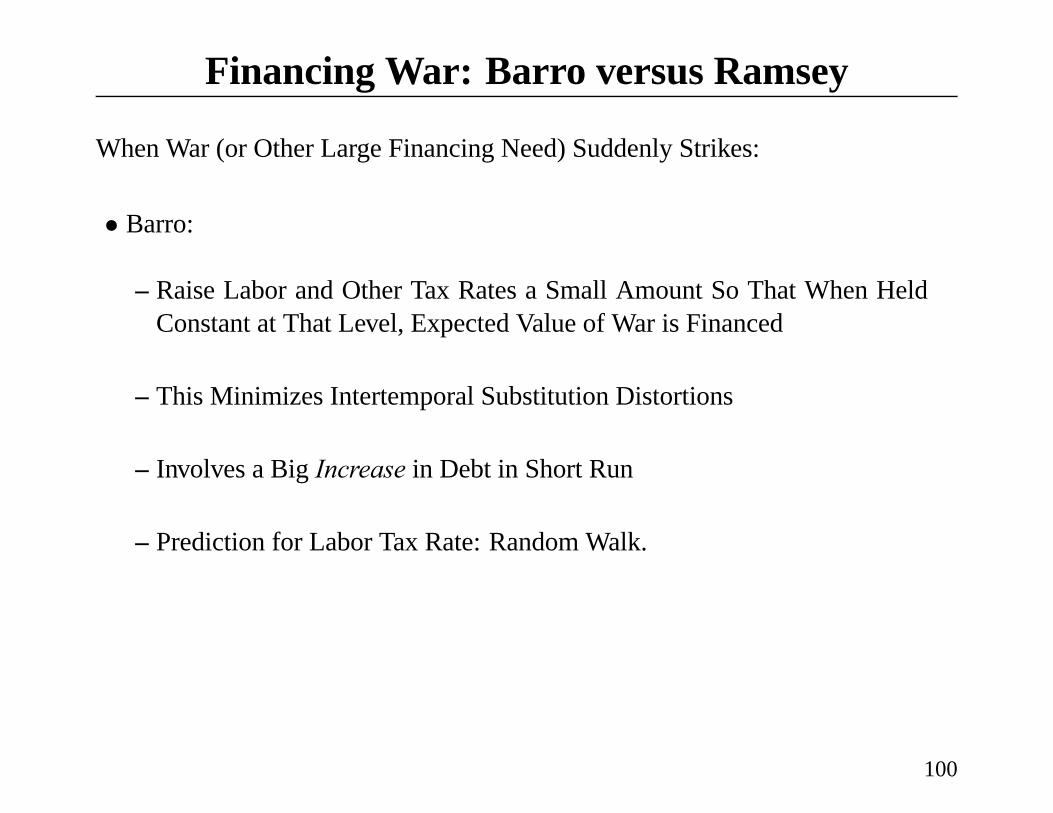
Financing War: Barro versus Ramsey

When War (or Other Large Financing Need) Suddenly Strikes:

• Barro:

– Raise Labor and Other Tax Rates a Small Amount So That When HeldConstant at That Level, Expected Value of War is Financed

– This Minimizes Intertemporal Substitution Distortions

– Involves a Big Increase in Debt in Short Run

– Prediction for Labor Tax Rate: Random Walk.

100

Financing War: Barro versus Ramsey ...

• Ramsey:

– Tax Existing Capital Assets (Human, Physical, etc) For Full Amount ofExpected Value of War. Do This at the First Sign of War.

– This Minimizes Intertemporal and Intratemporal Distortions (Don’t ChangeTax Rates on Income at all).

– Reduce Outstanding Debt

– Make Essentially No Change Ever to Labor Tax Rate

101

Financing War: Barro versus Ramsey ...

– Example:

∗ Suppose War is Expected to Last Two Periods, Cost: $1 Per Period

∗ Suppose Gross Rate of Interest is 1.05 (i.e., 5%)

∗ Tax Capital 1 + 1/1.05 = 1.95 Right Away.

∗ Debt Falls $0.95 in Period When War Strikes.

– Involves a Reduction of Outstanding Debt in Short Run.

– Prediction for Labor Tax Rate: Roughly Constant.

102

A Computational Issue

• Conditional On a Value for λ, Finding Ramsey Allocations Easy (Can UseSimple Linearization Procedures!)

• Policies Can Then Be Computed From Ramsey Allocations.

– Example: Labor Tax Rate Can Be Computed from Ramsey Allocations BySolving for τ t :

ul (ct, lt) + uc (ct, lt)× fn (kt, lt)× (1− τ t) = 0

• But, How To Get λ?

– Get it the Hard Way, Outlined Above

– Under Very Limited Conditions, can Calibrate λ

103

Calibrating the Multiplier, λ

• Conditional on λ :

– Nonstochastic Steady State Consumption, Capital Stock, Labor, Labor TaxRate Functions of λ :

c = c (λ) , l = l (λ)

– Steady State Policy Variable (debt, labor tax, capital tax rate) Can BeComputed:

τ (λ) = 1 +ul (c, l)

uc (c, l) fn (k, l)

• In Practice, τ (λ) is a Monotone Function of λ. Choose λ So That

τ = τ³λ´, τ ∼ Sample Average of Labor Tax Rate

104

Problem With Calibrating Multiplier

• Implicitly, this Assumes the Economy Was in an Optimal Policy Regime in theHistorical Sample

• Problem

– When People Compute Optimal Policy, they Want to be Open to thePossibility that Policy Outcomes are Not Optimal

– Want to Use the Ramsey-Optimal Policies as a Basis For RecommendingBetter Policies

• Still, Calibration of λ Works for an Analyst Who Seriously Entertains theHypothesis that Policy in the Sample Was Optimal

• Related to Woodford’s Idea of the Timeless Perspective

106

Optimal Monetary Policy When the IntertemporalBudget Constraint Does Not Bind

• Current Generation of Monetary Models Put Government Budget Constraint inBackground by Assuming Presence of Lump Sum Taxes to Balance Budget.

• Ramsey Optimal Policies in These Models Easy to Compute.• Outline:

– Simple, deterministic example– Simple example with uncertainty– General case.– Rotemberg sticky price example.

• Summary of:

[1] Levin, A., Lopez-Salido, J.D., 2004. "Optimal Monetary Policy withEndogenous Capital Accumulation", manuscript, Federal Reserve Board.

[2] Levin, A., Onatski, A., Williams, J., Williams, N., 2005. "Monetary Policyunder Uncertainty in Microfounded Macroeconometric Models." In: NBERMacroeconomics Annual 2005, Gertler, M., Rogoff, K., eds. Cambridge,

106

Optimal Monetary Policy When the Intertemporal Budget Constraint Does Not Bind ...

• Simple, deterministic example:

– Model: one equation characterizing the equilibrium of the private economy,and one for the policy rule.

– Private economy equation:

πt − βπt+1 − γyt = 0, t = 0, 1, ... (1)

– Want to do optimal policy. So throw away the policy rule.

– Have one equation, (1) in two unknowns, πt, yt. Need more equations!

– Optimization provides additional equations.

107


– Lagrangian Problem:

max{πt,yt;t=0,1,...}

∞Xt=0

βt{u (πt, yt) + λt [πt − βπt+1 − γyt]}

– Equations that characterize the optimum: (1), and first order conditions

∗ Fonc for yt :uy(πt, yt)− γλt = 0, t = 0, 1, ...

∗ Fonc for π0 :uπ (π0, y0) + λ0 = 0,

∗ Fonc for πt :

uπ (πt, yt) + λt − λt−1 = 0, t = 1, 2, ... .

108


– Issue:

∗ Fonc at t = 0 different than at t > 0

∗ Solution: define λ−1 ≡ 0 and our complete system of equations is, fort = 0, 1, 2, ... .

πt − βπt+1 − γyt = 0,

uπ (πt, yt) + λt − λt−1 = 0,

uy(πt, yt)− γλt = 0,

– We have added two equations and one new unknown, λt, with initialcondition, λ−1 = 0.

– System can be solved using standard solution methods.

109


– Compute Steady State:

uπ (π, y) + λ− λ = 0

uy (π, y)− γλ = 0

π − βπ − γy = 0.

– Linearize system around steady state and use undetermined coefficientmethod:

zt ≡

⎛⎝ ∆πt∆yt∆λt

⎞⎠ , ∆xt ≡ xt − x.

α0zt+1 + α1zt + α2zt−1 = 0,

– Use undetermined coefficient method, or some other method.

110


– Projection and perturbation methods:

∗ Policy rule:

π (λ−1) , λ (λ−1) , y (λ−1) .

– Functional Equations:

uπ (π (λ−1) , y (λ−1)) + λ (λ−1)− βλ−1 = 0

uy(π (λ−1) , y (λ−1))− γλ (λ−1) = 0

π (λ−1)− βπ [λ (λ−1)]− γy (λ−1) = 0

– Period t state: λt−1.

111


• Simple example with uncertainty:

–st ∈ (S1, ..., SN)

‘history’, st = (s0, s1, ..., st)

probability of st : µ¡st¢> 0.

– private sector equilibrium conditions:

π¡st¢− β

Xst+1|st

µ¡st+1

¢µ (st)

π¡st+1

¢− γy

¡st¢= 0, t = 0, 1, ...

112


– Lagrangian problem:

max{π(st),y(st)}all st

∞Xt=0

Xst+1|st

βµ¡st+1

¢{u¡π¡st¢, y¡st¢¢

+λ¡st¢⎡⎣π ¡st¢− β

Xst+1|st

µ¡st+1

¢µ (st)

π¡st+1

¢+ γy

¡st¢⎤⎦}

max{π(st),y(st)}all st

µ¡s0¢{u¡π¡s0¢, y¡s0¢¢

+λ¡s0¢⎡⎣π ¡s0¢− β

Xs1|s0

µ¡s1¢

µ (s0)π¡s1¢+ γy

¡s0¢⎤⎦}

+βXs1|s0

µ¡s1¢{u¡π¡s1¢, y¡s1¢¢

+λ¡s1¢⎡⎣π ¡s1¢− β

Xs2|s1

µ¡s2¢

µ (s1)π¡s2¢+ γy

¡s1¢⎤⎦} + ...

113


• First order conditions.

– Pick a particular history, s1 = (s0, s1) .

∗ Fonc for π¡s1¢:

βµ¡s1¢{uπ

¡π¡s1¢, y¡s1¢¢+ λ

¡s1¢}− µ

¡s0¢λ¡s0¢βµ¡s1¢

µ (s0)= 0,

or

uπ¡π¡s1¢, y¡s1¢¢+ λ

¡s1¢− λ

¡s0¢= 0,

∗ Fonc for y¡s1¢:

βµ¡s1¢uπ¡π¡s1¢, y¡s1¢¢+ βµ

¡s1¢λ¡s1¢γ = 0,

or,uπ¡π¡s1¢, y¡s1¢¢+ λ

¡s1¢γ = 0

115


– Reverting to simple notation,

πt − βEtπt+1 − γyt = 0,

uπ (πt, yt) + λt − λt−1 = 0,

uy(πt, yt)− γλt = 0

– Again, use standard methods to solve this.

116


• General Case– Economy without monetary policy rule: N − 1 private sector equilibrium

conditions -

(+)Xst+1|st

µ¡st+1

¢µ (st)

f

⎛⎝x¡st¢| {z }

N×1

, x¡st+1

¢| {z }N×1

, st, st+1

⎞⎠ = 0|{z}(N−1)×1

– Lagrangian

max{x(st)}all st

∞Xt=0

βtXst

µ¡st¢{U¡x¡st¢, st¢

+ λ¡st¢| {z }

1×(N−1)

Xst+1|st

µ¡st+1

¢µ (st)

f¡x¡st¢, x¡st+1

¢, st, st+1

¢| {z }(N−1)×1

}

– Fonc for x (st) :

(∗) U1¡x¡st¢, st¢| {z }

1×N

+ λ¡st¢| {z }

1×N−1

Xst+1|st

µ¡st+1

¢µ (st)

f1¡x¡st¢, x¡st+1

¢, st, st+1

¢| {z }N−1×N

+β−1λ¡st−1

¢| {z }1×N−1

f2¡x¡st−1

¢, x¡st¢, st−1, st

¢| {z }N−1×N

= 0|{z}1×N

117


• Equations:N − 1 priate sector equilibrium conditions, (+)

N first order conditions for Ramsey problem. (∗)• Unknowns:

N endogenous variables to be determined

N − 1 multipliers.• Can solve this in the usual way, but be aware of two issues:

– Ramsey Fonc’s require differentiating household first order conditions (apain!)

– Steady state a little trickier to compute.

118


• Strategy for finding steady state of multipliers and x.– Fix one element of x, say it’s π.∗ There remain N − 1 unknowns in x.∗ Find these by solving steady state of (+) (this is the usual steady state -

solving problem)∗ Solve (∗) for the steady state multipliers:

U1|{z}1×N

+ λ|{z}1×(N−1)

£f1 + β−1f2

¤| {z }(N−1)×N

= 0,

∗WriteY = U 01X =

£f1 + β−1f2

¤0β = λ0,

∗ Then (‘regression withN observations andN−1 explanatory variables’):β = (X 0X)

−1X 0Y

u = Y −Xβ,

S = u0u.

∗ Select π until S (π) = 0.

119


• Good news!

• Levin, A., Lopez-Salido, J.D., (2004). and Levin, A., Onatski, A., Williams,J., Williams, N., (2005) simplified two very unpleasant steps in the abovecomputations. They wrote programs which

– take u, β and f as input and writes (*) in Dynare format

– take u, β and f as input and writes out mapping from x to S in Dynareformat.

120


• Rotemberg Sticky Price example– Household

maxE0

∞Xt=0

βtnlog (Ct)−

χ

2h2t

o,

s.t.Bt

Pt= (1 +Rt−1)

Bt−1Pt− Ct +

Wt

Ptht + Πt.

– First order conditions:χhtCt =

Wt

Pt,

1

1 +Rt= βEt

PtCt

Pt+1Ct+1

– Final output, Yt, produced by competitive firms with technology:

Yt =

∙Z 1

0

Cj,tθ−1θ di

¸ θθ−1

, θ ≥ 1, FONC: Cj,t =

µPj,t

Pt

¶−θCt.

121


– Intermediate good firm j period t revenues and marginal cost:

(1 + τ )Pj,t

PtCj,t −MCt × Cj,t −

φ

2

µPj,t

Pj,t−1− 1¶2

Ct,

MCt =Wt

Pt

1

exp (Zt)

µ=

χhtCt

exp (Zt)

¶.

– Intermediate good firm j Lagrangian problem:

max{Pj,t+n}∞n=0

Et

∞Xn=0

βn Ct

Ct+n[(1 + τ )

µPj,t+n

Pt+n

¶1−θCt+n

−MCt+n ×µPj,t+n

Pt+n

¶−θCt+n −

φ

2

µPj,t+n

Pj,t−1+n− 1¶2

Ct+n],

122


– Firm fonc, after imposing Pit = Pjt, all i, j (all firms behave identically inequilibrium) and equilibrium condition on MCt

(FONC)∙τ − 1

(θ − 1)

¸(1− θ) + θ

µχhtCt

exp (Zt)− 1¶

−φ (πt − 1)πt + βEtφ (πt+1 − 1)πt+1 = 0.

– Resource constraint:

(resource) Ct

∙1 +

φ

2(πt − 1)2

¸= Yt = exp (Zt)ht.

– Solution to Ramsey problem when τ = 1/ (θ − 1) is obvious

πt = 1, χh2t = 1, Ct = exp (Zt)ht.

∗ Delivers the best outcomes in the economy with no price frictions. Can’tbeat that!∗ Verify that with Lagrangian approach to Ramsey, get same answer.

123

optimal fiscal and monetary policy

Documents