optimal fuzzy pid c tuned with g...

OPTIMAL FUZZY PID

CONTROL TUNED WITH

GENETIC ALGORITHMS

Carlos Miguel Almeida Santos

Master in Computer and Electrical Engineering

Area of Specialization in Automation and Systems

Department of Electrical Engineering

Institute of Engineering of Porto

2013

This report fulfil, partially, the needs that are in the Unit Course of Thesis, of the 2º year,

of Master in Computer and Electrical Engineering

Candidate: Carlos Miguel Almeida Santos, Nº 1090033, [email protected]

Scientific orientation: Professor Doctor Ramiro de Sousa Barbosa, [email protected]

Master in Computer and Electrical Engineering

Area of specialization in Automation and Systems

Department of Electrical Engineering

Institute of Engineering of Porto

5 de November de 2013

I dedicate this work to my family and special to my wife.

i

Acknowledgments

To Institute of Engineering of Porto for having accepted me as a Master student.

A special recognition to my supervisor Professor Doctor Ramiro de Sousa Barbosa for

accepting me as his M.Sc. student, for the support, dedication and guidance during the

period of my thesis.

I also want to thank my wife for all support and tolerance during this stage and finally I

also want to give a special thank to my parents in law that also support me all time.

iii

Abstract

Fuzzy logic controllers (FLC) are intelligent systems, based on heuristic knowledge, that

have been largely applied in numerous areas of everyday life. They can be used to describe

a linear or nonlinear system and are suitable when a real system is not known or too

difficult to find their model. FLC provide a formal methodology for representing,

manipulating and implementing a human heuristic knowledge on how to control a system.

These controllers can be seen as artificial decision makers that operate in a closed-loop

system, in real time.

The main aim of this work was to develop a single optimal fuzzy controller, easily

adaptable to a wide range of systems – simple to complex, linear to nonlinear – and able to

control all these systems. Due to their efficiency in searching and finding optimal solution

for high complexity problems, GAs were used to perform the FLC tuning by finding the

best parameters to obtain the best responses.

The work was performed using the MATLAB/SIMULINK software. This is a very useful

tool that provides an easy way to test and analyse the FLC, the PID and the GAs in the

same environment. Therefore, it was proposed a Fuzzy PID controller (FL-PID) type

namely, the Fuzzy PD+I. For that, the controller was compared with the classical PID

controller tuned with, the heuristic Ziegler-Nichols tuning method, the optimal Zhuang-

Atherton tuning method and the GA method itself. The IAE, ISE, ITAE and ITSE criteria,

used as the GA fitness functions, were applied to compare the controllers performance

used in this work.

Overall, and for most systems, the FL-PID results tuned with GAs were very satisfactory.

Moreover, in some cases the results were substantially better than for the other PID

controllers. The best system responses were obtained with the IAE and ITAE criteria used

to tune the FL-PID and PID controllers.

Keywords

Fuzzy, intelligent systems, heuristic, control, optimal, GA, PID.

v

Resumo

Os Controladores Lógicos Difusos (CLD) são sistemas inteligentes, baseados em

conhecimentos heurísticos, que têm vindo a ser amplamente aplicados em inúmeras áreas

do quotidiano. Podem ser usados para descrever sistemas lineares ou não-lineares,

tornando-se apropriados quando se desconhece o modelo do sistema real ou no caso de o

sistema ser difícil de modelar. Os CLD apresentam uma metodologia formal para

representar, manipular e implementar um conhecimento heurístico de como controlar um

sistema. Estes controladores funcionam como gestores artificiais de decisão que operam

em sistemas de malha-fechada, e em tempo real.

O principal objetivo deste trabalho consistiu no desenvolvimento de um único controlador

difuso ótimo, facilmente adaptável a uma vasta gama de sistemas – simples a complexos,

lineares a não-lineares – e com capacidade para controlar sistemas distintos. Devido à sua

eficácia na procura e descoberta de soluções ótimas, para sistemas de elevada

complexidade, os Algoritmos Genéticos (AG) foram usados para a sintonia do CLD

através da procura dos melhores parâmetros por forma a encontrar as melhores respostas.

O trabalho foi realizado usando o software MATLAB/SIMULINK. Esta é uma ferramenta

útil que permite facilmente testar e analisar, no mesmo ambiente, o CLD, o PID e os AG.

Por esta razão, foi proposto um controlador difuso do tipo PID, concretamente o

Controlador Lógico Difuso PD+I (CLD-PID). Este controlador foi comparado com o

controlador PID clássico sintonizado com o método heurístico de Ziegler-Nichols, o

método ótimo de sintonização de Zhuang-Atherton e o próprio método de AG. Os critérios

IAE, ISE, ITAE e ITSE, usados como as funções de avaliação dos AG, foram utilizados

para comparar os desempenhos dos controladores usados neste trabalho.

vi

De um modo geral, e para a maioria dos sistemas, os resultados do CLD-PID sintonizados

com os AG foram bastantes satisfatórios. Para além disso, em alguns casos, os resultados

foram consideravelmente melhores do que para os restantes controladores PID. As

melhores respostas de sistemas foram obtidas com os critérios IAE e ITAE, que foram

usados para sintonizar os controladores CLD-PID e PID.

Palavras-Chave

Lógica Difusa, sistemas inteligentes, heurística, controlo, ótimo, AG, PID.

vii

Contents

ACKNOWLEDGMENTS ................................................................................................................................ I

ABSTRACT ................................................................................................................................................... III

RESUMO ......................................................................................................................................................... V

CONTENTS ................................................................................................................................................. VII

TABLE OF FIGURES .................................................................................................................................. IX

INDEX OF TABLES .................................................................................................................................. XIII

ACRONYMS ................................................................................................................................................ XV

1. INTRODUCTION .................................................................................................................................. 1

1.1. CONTEXTUALIZATION....................................................................................................................... 3

1.2. OBJECTIVES ...................................................................................................................................... 3

1.3. SCHEDULING ..................................................................................................................................... 3

1.4. OUTLINE OF THE THESIS .................................................................................................................... 4

2. FUZZY CONTROL SYSTEMS ............................................................................................................ 5

2.1. FUZZY SETS ...................................................................................................................................... 6

2.2. FUZZY LOGIC CONTROL ................................................................................................................. 13

2.2.1. Fuzzification Interface........................................................................................................... 14

2.2.2. Rule-Base .............................................................................................................................. 14

2.2.3. Inference Mechanism ............................................................................................................ 15

2.2.4. Defuzzification Interface ....................................................................................................... 17

2.2.5. Fuzzy Mechanism Example ................................................................................................... 20

2.3. FUZZY PID CONTROLLER ............................................................................................................... 21

2.3.1. Design of Fuzzy PID controllers ........................................................................................... 23

2.4. MATLAB FUZZY LOGIC TOOLBOX ................................................................................................ 23

3. GENETIC ALGORITHMS ................................................................................................................. 35

3.1. TYPES OF ENCODING ...................................................................................................................... 38

3.1.1. Binary Encoding .................................................................................................................... 38

3.1.2. Many-Character and Real-Valued Encodings ...................................................................... 39

3.1.3. Tree Encoding ....................................................................................................................... 40

3.2. GENETIC ALGORITHMS ................................................................................................................... 40

3.3. DESIGNING GENETIC ALGORITHM PRINCIPLES ............................................................................... 41

3.4. SIMPLE GENETIC ALGORITHM ........................................................................................................ 41

3.5. SELECTION METHODS ..................................................................................................................... 43

3.5.1. Proportional Selection .......................................................................................................... 44

viii

3.5.2. Random Selection .................................................................................................................. 45

3.5.3. Rank Selection ....................................................................................................................... 45

3.5.4. Tournament Selection ............................................................................................................ 46

3.5.5. Stochastic Sampling Selection ............................................................................................... 46

3.6. CROSSOVER ..................................................................................................................................... 46

3.7. MUTATION ...................................................................................................................................... 48

3.8. REPLACEMENT ................................................................................................................................ 49

3.9. STOPPING CRITERIA ........................................................................................................................ 50

3.10. RESTRICTIONS ................................................................................................................................. 51

3.11. MATLAB GLOBAL OPTIMIZATION TOOLBOX ................................................................................ 52

4. OPTIMAL TUNING OF FUZZY PID CONTROLLERS ................................................................. 55

4.1. BENCHMARK SYSTEMS .................................................................................................................... 55

4.2. PERFORMANCE INDICES .................................................................................................................. 57

4.3. PID CONTROLLER ........................................................................................................................... 58

4.4. FUZZY LOGIC PID CONTROLLER ..................................................................................................... 62

4.5. STRUCTURE OF THE GENETIC ALGORITHM ...................................................................................... 67

4.6. SIMULATION AND RESULTS ............................................................................................................. 70

4.6.1. System 1 ................................................................................................................................. 70

4.6.2. System 2 ................................................................................................................................. 74

4.6.3. System 3 ................................................................................................................................. 77

4.6.4. System 4 ................................................................................................................................. 81

4.6.5. System 5 ................................................................................................................................. 85

4.6.6. System 6 ................................................................................................................................. 89

4.7. CONTROLLERS RESULTS AND DISCUSSION ...................................................................................... 93

5. CONCLUSIONS .................................................................................................................................... 95

REFERENCES ............................................................................................................................................... 97

ix

Table of Figures

Figure 1 Characteristic function of the classical (crisp) set A. ..................................................... 7

Figure 2 Membership function of the fuzzy set A. ....................................................................... 7

Figure 3 Union of two fuzzy subsets using maximum operator. ................................................... 8

Figure 4 Interception of two fuzzy sets using the minimum operator (a) and algebraic product

(b). 9

Figure 5 Complement of a fuzzy set. ............................................................................................ 9

Figure 6 Core, support and boundary of a fuzzy set. .................................................................. 10

Figure 7 Normal (a) and Subnormal (b) fuzzy sets. ................................................................... 11

Figure 8 Convex (a) and non-convex (b) fuzzy sets. .................................................................. 11

Figure 9 Commonly used membership functions [13]. .............................................................. 12

Figure 10 Fuzzy control system [10]. ........................................................................................... 13

Figure 11 Centre of gravity method. ............................................................................................. 18

Figure 12 Centre average method. ................................................................................................ 19

Figure 13 Mean of maxima method. ............................................................................................. 19

Figure 14 Example of fuzzification, Mamdani’s inference and defuzzification. .......................... 20

Figure 15 Typical PID control diagram. ....................................................................................... 22

Figure 16 Typical Fuzzy PID control diagram. ............................................................................ 22

Figure 17 Triangular membership function example (trimf). ................................................... 24

Figure 18 Trapezoidal membership function example (trapmf). .............................................. 25

Figure 19 Simple Gaussian membership function example (gaussmf). .................................... 25

Figure 20 Two-sided Gaussian membership function example (gauss2mf). ............................ 26

Figure 21 Generalized Bell membership function example (gbellmf). .................................... 26

Figure 22 Basic Sigmoidal membership function example (sigmf). ......................................... 27

Figure 23 Sigmoidal difference membership function example (dsigmf). ................................ 27

Figure 24 Sigmoidal product membership function example (psigmf). .................................... 28

Figure 25 Polynomial Z membership function example (zmf). ................................................... 28

Figure 26 Polynomial S membership function example (smf). ................................................... 29

Figure 27 Polynomial Pi membership function example (pimf). ............................................... 29

Figure 28 MATLAB Fuzzy Inference System editor graphical interface. ................................... 30

Figure 29 MATLAB Membership Function Editor graphical interface. ...................................... 31

Figure 30 MATLAB Rule Editor graphical interface. .................................................................. 31

Figure 31 MATLAB Rule Viewer graphical interface. ................................................................ 32

Figure 32 MATLAB Surface Viewer graphical interface. ........................................................... 33

Figure 33 Example of a binary encoding. ..................................................................................... 38

x

Figure 34 Example of an octal encoding. ..................................................................................... 39

Figure 35 Example of a hexadecimal encoding. ........................................................................... 39

Figure 36 Example of real numbers permutation encoding. ......................................................... 39

Figure 37 Example of a value encoding. ...................................................................................... 40

Figure 38 Example of a simple Genetic Algorithm flowchart. ..................................................... 42

Figure 39 Example of a roulette wheel selection method [23]. .................................................... 45

Figure 40 Example of search space with restrictions and feasible region. ................................... 51

Figure 41 Genetic algorithm solver graphical interface................................................................ 54

Figure 42 Block diagram of the PID control system. ................................................................... 58

Figure 43 Block Diagram of the Fuzzy PD+I control system....................................................... 63

Figure 44 Gaussian membership functions of inputs (a) and output (b). ...................................... 65

Figure 45 Output control surface. ................................................................................................. 66

Figure 46 Fuzzy inference system. ............................................................................................... 66

Figure 47 Step response of System 1. ........................................................................................... 70

Figure 48 Evolution of best fitness for the IAE (a), ISE (b), ITAE (c) and ITSE (d) criteria

regarding System 1. .................................................................................................................. 71

Figure 49 Step responses of System 1 according to IAE (a), ISE (b), ITAE (c) and ITSE (d)

criteria. 73





criteria. 77





criteria. 81





criteria. 85




Figure 61 1 second impulse responses of System 5 according to IAE (a), ISE (b), ITAE (c) and

ITSE (d) criteria........................................................................................................................ 89

Figure 62 SIMULINK block diagram of System 6. ..................................................................... 90


xi




criteria. 93

xiii

Index of Tables

Table 1 Scheduling of the developed project. ............................................................................. 3

Table 2 Fuzzy rule-base for output u(t). .................................................................................... 15

Table 3 Correspondence between genetics and genetic algorithms concepts. .......................... 37

Table 4 PID controller parameters obtained from the ZN methods [28]. .................................. 60

Table 5 PID controller parameters using ZA setpoint method [28]. ......................................... 61

Table 6 Fuzzy rule-base for output. ........................................................................................... 64

Table 7 GA parameters used in all simulations. ........................................................................ 68

Table 8 GA upper bounds and initial population used for System 1 simulations. .................... 71

Table 9 Results of Fuzzy PID tuned with GAs for System 1. ................................................... 72

Table 10 Results of PID tuned with ZN, ZA and GAs methods for System 1. ........................... 72












Table 22 Results of PID tuned with GAs method for System 5. ................................................. 88



Table 25 Results of PID tuned with GAs methods for System 6. ............................................... 92

xv

Acronyms

BOA – Bisector of Area

CA – Centre Average

CC – Cohen and Coon

CHR – Chien, Hrones and Reswick

COA – Centre of Area

COG – Centre of Gravity

CPU – Central Processing Unit

FIS – Fuzzy Inference System

FLC – Fuzzy Logic Controller

FL-PID – Fuzzy Logic-Proportional Integral Derivative

FOPDT – First Order Plus Dead Time

GA – Genetic Algorithm

GOT – Global Optimization Tool

GUI – Graphical User Interface

IAE – Integral of Absolute Error

ISE – Integral of the Square of the Error

ITAE – Integral Time Multiplied by the Absolute Error

ITSE – Integral of Time Multiplied by the Squared Error

xvi

IST2E – Integral Squared Time-squared weighted Error

LM – Leftmost Maximum

MOM – Mean of Maxima

NB – Negative Big

NM – Negative Medium

NN – Neural Networks

NS – Negative Small

OX – Ordered Crossover

PB – Positive Big

PC – Personal Computer

PID – Proportional Integrative Derivative

PM – Positive Medium

PMX – Partially Mapped Crossover

PPX – Precedent Preservative Crossover

PS – Positive Small

RAM – Random Access Memory

RM – Rightmost Maximum

Z – Zero

ZA – Zhuang-Atherton

ZN – Ziegler-Nichols

1

1. INTRODUCTION

Control is present in several areas of knowledge such as science and engineering. It is used

to control processes like for example the control of a car steering wheel to ensure that a car

is in the right path. In industry numerous conditions such as pressure, temperature, speed,

robot arms or motor positioning need to be constantly controlled and monitored in order to

maintain all processes in the desired state [1][2].

Overall, there are two types of control – closed-loop control and open-loop control. In

closed-loop control the output is measured and compared with a reference. In this case the

control is applied to the input in order to reduce the difference between the output and the

reference to zero, i.e., ideally the error is zero. Concerning the open-loop control the output

is not measured and in the case of disturbances the system does not react as expected

requiring a proper calibration to make sure that the system reacts according to planned.

This type of control is used when the relation between inputs and outputs is well known

and there are no disturbances [1].

Classical Proportional Integrative Derivative (PID) is the most used control technique,

applied 95% of the times, since it is easier to implement, has a good response in transient

and steady-state and presents very satisfactory results in several industrial applications.

This control has three variables that must be tuned: the Proportional (P), the Integrative (I)

and the Derivative (D) actions. The proportional action actuates proportionally to the error;

the Integrative action has a stronger influence in the error reduction at the steady-state;

while, the Derivative action has a strong influence in stability. It is important to mention

that these three variables are dependent from each other [3][4].

2

With the need for more efficient control systems other control techniques have been

developed such as Fuzzy Logic Control (FLC) or Neural Networks (NN). In the last

decades it has been observed a growing interest on fuzzy controllers due to their important

value for controlling complex and nonlinear industrial processes. Since the introduction of

the Fuzzy Set Theory many advances have been made such as the combination of PID with

fuzzy systems. In fact over the years these FLC have proven their efficiency. Opposite to

classical control, fuzzy logic systems are based on heuristic knowledge rather than exact

mathematics. This type of control is used to describe a linear or nonlinear system. By using

this methodology, fuzzy controllers become easier to design since they use verbal language

such as hot, very hot or cold rather than exact values. Therefore, it is possible to design a

fuzzy controller for high performance control, even without knowing the model. Moreover,

an interesting characteristic of these systems is their ability to handle numeric and

linguistic information in the same framework. Fuzzy systems can evaluate a linguistic

information and transpose it to exact numbers for later treatment in a computer

[5][6][7][8].

Several techniques have been applied to find a balance and equilibrium in fuzzy systems.

One of the most recent techniques is based on the combination of Fuzzy PID control

systems with Genetic Algorithms (GAs) leading to hybrid systems.

Genetic Algorithms (GAs) are based on the Natural Selection Principle theory proposed by

a biologist named Charles Darwin (1859). This theory holds the fundamental idea that the

most capable and environmentally adapted individuals survive and reproduce while the

less able tend to die and disappear. GAs are used to find and search for minimums or

maximums in a specific proposed problem. In fact, after a few interactions (generations)

the best solutions are find [9]. Thus, the evolutionary techniques used in GAs can be

combined with Fuzzy PID Systems to help find the optimal parameters of the controller.

The main advantage is that the designer does not need to know the process since GAs will

adapt and tune the controller based on the system response; in that way this hybrid

controller can be used for any given system.

The main goal of this study is to develop a system that will be able to control several

systems using the same controller. For that, it will be used a hybrid system containing a

PID Fuzzy Logic Controller combined with GAs. GAs were chosen due to their simplicity

3

and efficacy [9]. The concept is to develop an auto-adaptable fuzzy PID controller by

applying the FLC, the PID and the GAs to find the optimum parameters.

1.1. CONTEXTUALIZATION

In industry there are many nonlinear processes that are difficult to model in order to

achieve the proposed objectives using a PID controller. To successfully control a process it

is possible to use an independently tuned FLC which is expensive and time consuming. It

is important to use a control that has the ability to adapt to all processes without the need of

developing a mathematical model and thus save time of the developer. An optimal fuzzy

PID controller, can be a good solution, and can be achieved with the proposed project.

1.2. OBJECTIVES

The main objective of this project is to design an optimal fuzzy PID controller using GA,

and MATLAB as a developing tool. The controller will be tested in six different systems

with distinct responses in order to verify its efficiency and compared with a classical PID

controller.

1.3. SCHEDULING

In Table 1 it is possible to observe the scheduling concerning the tasks performed during

the development of this project (semester).

Table 1 Scheduling of the developed project.

Stage

Duration

(weeks) March April May June July August September October November

Control Theory Study 4

FL Study 4

GA Study 4

MATLAB Study 4

FLC development 6

GA development 5

Tests and results 15

Report writing 20

Thesis presentation 1

4

1.4. OUTLINE OF THE THESIS

This thesis is outlined as follows. Chapter 1 presents some basic concepts of control

systems, the scope and proposal of the work, and the outline of the thesis. Chapter 2

introduces the fundamentals of fuzzy logic control systems. Moreover, the MATLAB

Fuzzy Toolbox operation is described and explained. In Chapter 3 Genetic Algorithms

theory is presented as well as their fundamental concepts. In this chapter the genetic

algorithm toolbox from the MATLAB Global Optimization Toolbox is briefly introduced.

The obtained results and their discussion are described in Chapter 4. The conclusions are

summarized in Chapter 5 as well future perspectives of work.

5

2. FUZZY CONTROL

SYSTEMS

Fuzzy logic was first proposed by Lotfi A. Zadeh in 1965 [8]. This type of controllers is

based on the idea that Humans do not think in terms of exact numbers but rather in

concepts. One of the first experiences performed with fuzzy controllers revealed that the

control of a vapour machine with a simple fuzzy controller was very efficient [8].

Fuzzy logic is a tool that uses ambiguous information such as hot, high or fast normally in

a language that is easily understood by humans, and then converted into a numerical value

that can be manipulated by a microprocessor or computer [8][10].

The implementation of a fuzzy control is appropriate when the modelling of a real world

system is too difficult and when the process is very well known in terms of human

experience. The development of a relatively accurate model of a dynamic system is very

complex to be used in controller development, mostly in the case of conventional design

control procedures that require restrictive plant assumptions such as linearity. Therefore,

conventional controllers are frequently developed using simple process models behaviour

that satisfies the required assumptions. Nevertheless, it is known that heuristics are present

in conventional control design processes as long as the actual implementation of the

6

control system is considered. Conventional control engineering that uses appropriate

heuristics to the design has been relatively successful. Fuzzy control provides a formal

methodology to represent, manipulate and implement a heuristic of human knowledge on

how to control a system [10].

2.1. FUZZY SETS

Fuzzy sets are classes with a continuous grade of membership. A class contains objects

with a certain grade of membership between the interval . Contrary to conventional

sets, where a number belong or not to that set, in fuzzy sets that number can partially

belong to it, this means that a number belongs to the fuzzy set according to the

membership of the variable. In fuzzy logic the variables are names, instead of numbers. As

an example, in the case of temperature control, temperature is the linguistic variable which

can take linguistic values like hot or cold. This kind of approach has more meaning in

terms of human thought because humans tend to think in names rather than numbers.

Another concept is the membership function that represents the way in which linguistic

values belong to a fuzzy set for that linguistic value. This function must be defined in order

to better fits the physical meaning of the problem in question [5][8][11].

The universe of discourse consist in all possible elements of concern in a particular

context. Each of these elements are called a member, or an element of the universe of

discourse [10][11].

For any classical set, the characteristic function of a set is defined by

(1)

The characteristic function of the classical set defined above is an indicator of

members and non-members of the classical (crisp) set , there is no ambiguity or grade of

membership. An example of a classical set is shown in Figure 1.

7

Figure 1 Characteristic function of the classical (crisp) set A.

With fuzzy sets the characteristic function must be generalized since in fuzzy sets there

might be an element that can partially belong to that set or not partially belong to it. In this

case larger values denote a higher degree of membership. We have to notice that the

maximum degree of membership is 1, and in this case the value completely belongs to that

fuzzy set, on the other hand, the minimum value is 0, and this is the case where the value

does not belong to that fuzzy set. So, to generalize the characteristic function, the

membership function needs to be defined in association with each set in the universe of

discourse. A fuzzy set (2) is defined as an ordered pair , where is the universe of

discourse and is the a set membership function mapping onto the interval .

(2)

In fuzzy logic every set can have different membership functions, the function that better

describes that set. Therefore, that function should describe the better way possible the

characteristic represented by the set.

An example of a membership function of a fuzzy set is represented in Figure 2.

Figure 2 Membership function of the fuzzy set A.

8

Like in classical sets, operations can be performed between sets, the standard operations

between fuzzy sets are, the union, intersection and complement operations.

Union

(3)

(4)

(5)

The union standard operation of two fuzzy sets can be done using the maximum operator

(3) or the algebraic sum (5), although, other union operations are possible. An example of

the union operation between two fuzzy sets using the maximum operator is shown in Figure

3.

Figure 3 Union of two fuzzy subsets using maximum operator.

Intersection

(6)

(7)

The intersection operation of two fuzzy sets can be done using the minimum operator (6) or

the algebraic product (7), although, other intersection operations can be performed. An

example of the intersection operation between two fuzzy sets using the minimum operator

and the algebraic product are shown in Figure 4.

9

Figure 4 Interception of two fuzzy sets using the minimum operator (a) and algebraic product

(b).

Complement

(8)

The complement standard operation (8) is the same as the inverse of fuzzy set . An

example of the complement operation of a fuzzy set is shown in Figure 5.

Figure 5 Complement of a fuzzy set.

There are more operations rather than the standard fuzzy operations. The aggregation

operations consist in combining several fuzzy sets into only one fuzzy set. These

operations of aggregation use the associative property that gives them the possibility to

extend their definitions to more than three arguments. Other common operations of

aggregation such as averaging operations and ordered weighted averaging operations are

also found in some literature. The use of these operations of aggregation is useful to fulfil

the space between the minimum operator, the intersection; and the maximum operator, the

union [12].

10

In fuzzy sets, the Morgan’s principals for classical sets are also valid. The properties of the

classical sets are also valid, except for the excluded middle axioms since fuzzy sets and

their complements can overlap. All the properties applied to classical sets are also used for

fuzzy sets. Moreover, due to this and the fact that a classical set are a subset of the interval

classical sets are a particular case of fuzzy sets [4].

The membership function describes the information in a fuzzy set, therefore the core of a

membership function for some fuzzy set is defined as that region of the universe that is

characterized by complete and full membership in that set. The core comprises those

elements of the universe such that . The support of a membership function for

some fuzzy set is defined as the region of the universe that is characterized by nonzero

membership in that set. The support comprises those elements of the universe such that

. The boundaries of a membership function for some fuzzy set are defined as the

region of the universe containing elements that have a nonzero membership but not

complete membership. The boundaries comprise those elements of the universe such that

. These elements of the universe are those with some degree of fuzziness,

or only partial membership in the fuzzy set. Figure 6 represents the universe regions that

comprises the core, support and boundaries of a typical fuzzy set [12].

Figure 6 Core, support and boundary of a fuzzy set.

The most common forms of membership functions are the normal and convex ones.

However, many operations on fuzzy sets, or operations on membership functions, result in

fuzzy sets that are subnormal and non-convex [12].

A fuzzy set is said to be normal only if the membership function has at least one element

of value one, i.e., the maximum value in a normalized universe. If the membership

11

function has one and one only element with the unity value, this element is typically

referred to as the prototype of the set [12].

A fuzzy set is said to be convex if the membership function elements are strictly

monotonically increasing, or strictly monotonically decreasing, or monotonically

increasing then strictly monotonically decreasing. In a formal way, for any given element

, , and in a fuzzy set, with the relation that respects the statement (9) than

it can be said that the fuzzy set is convex [12].

(9)

In Figure 7 is represented an example of normal and subnormal fuzzy sets, and in Figure 8

is represented an example of convex and non-convex fuzzy sets.

Figure 7 Normal (a) and Subnormal (b) fuzzy sets.

Figure 8 Convex (a) and non-convex (b) fuzzy sets.

Membership functions can be symmetrical or asymmetrical and are typically defined based

on one-dimensional universe although can be described on multidimensional universes. In

two dimensions curves become surfaces and for three or more dimensions these surfaces

12

become hyper-surfaces. These hyper-surfaces, or curves, are simple mappings of

parameters’ combinations in n-dimensional space to a membership value on interval .

Once again, this membership value expresses the membership degree that the specific

combination of parameters, in the n-dimensional space, has in a particular fuzzy set

defined on the n-dimensional universe of discourse. The hyper-surfaces for a n-

dimensional universe are analogous to joint probability density functions; but, of course,

the mapping for the membership function is to membership, in a particular set and not to

relative frequencies, as it is for probability density functions [12].

In fuzzy logic the selection of the membership functions is based on a subjective choice.

Therefore, the correct and best way to choose the membership function depends on the

designer knowledge and experience on the system in question. Figure 9 shows some

examples of the most commonly used memberships [11][13].

Figure 9 Commonly used membership functions [13].

13

2.2. FUZZY LOGIC CONTROL

To design a fuzzy controller it is necessary to collect information on how the artificial

decision maker should act in a closed-loop system. This information can come from a

human decision maker who performs the control task or the control designer begin

understanding the process dynamics and writing a set of rules on how to control the system

[10].

The fuzzy control block diagram represented in Figure 10 shows a fuzzy controller

embedded in a closed-loop control system. The outputs of the system are denoted by y(t),

their inputs by u(t), and the fuzzy controller reference input as r(t).

Figure 10 Fuzzy control system [10].

The fuzzy controller has four main components:

1. The fuzzification interface simply modifies the inputs so that they can be interpreted and

compared to the rules in the rule-base.

2. The inference mechanism evaluates which control rules are relevant at the current time

and then decides what should be the input to the system.

3. The rule-base holds the knowledge, in the form of a set of rules, in the best way to

control the system.

4. The defuzzification interface converts the conclusions reached by the inference

mechanism into the inputs to the system.

14

2.2.1. FUZZIFICATION INTERFACE

The fuzzification interface is the transformation process in which the crisp inputs values are

turned into fuzzy linguistic values. Such transformation is realized by introduction of the

membership functions, which define both a range of value and a degree of membership.

For linguistic variables it is important not only which membership function a variable

belongs to, but also a relative degree to which it is a member. A variable can have a

weighted membership in several membership functions at the same time because of the

memberships overlapping. A certain overlap between membership functions is desirable to

prevent the controller to be in poorly defined states, consequently returning output values

not well defined, leading to poor control [5][13].

If the process or measurement of the values has noise, it could be necessary to create fuzzy

sets for the measured values. In this case, the measured values could contain some errors

because of the noise, and can be converted into fuzzy sets that reflect their degree of

undependability, this may be useful but is not essential and can be ignored due to its

simplicity. Of course, in many cases the measurement noise can be low or not taken into

account, and in these cases, the fuzzification stage consists in create singleton membership

functions at the measured values, which simplifies the fuzzification mechanism

[5][10][14].

2.2.2. RULE-BASE

Humans tend to make decisions based on rules in the form of IF…THEN. In classical

logic, there are 4 most frequently rules based on IF…THEN; the modus ponendo ponens

from the Latin that means “mode that affirms by affirming” or modus ponens, the modus

tollendo tollens from the Latin, that means “mode that denies by denying”, or modus

tollens, the modus ponendo tollens from the Latin, that means “mode that denies by

affirming” and the modus tollendo ponens from the Latin, that means “mode that affirms

by denying”. The IF…THEN modus ponendo ponens form is the most frequently used

rules in fuzzy control [5][11].

The fuzzy rules are used in fuzzy control to define the relation between the fuzzified inputs

of the system and their outputs. This collection of rules is called the rule-base and it comes

in the form of IF premise THEN consequent. The premise or antecedent is associated with

the fuzzy controller inputs, on the other hand, the consequents or actions are associated

15

with fuzzy controller outputs. Each of this premise can be a conjunction of more than one

term. For instance, IF input a is HIGH AND input b is LOW THEN output c is HIGH.

The number of premises and consequents are limited by the number of inputs and outputs

and their linguistic values [10]. Table 2 shows an example of a rule base in a form of a

table with two input variables, error and error variation

, and one output .

In this example there are seven linguistic variables for each input, namely the Negative Big

(NB), the Negative Medium (NM), the Negative Small (NS), the Zero (Z), the Positive

Small (PS), the Positive Medium (PM) and the Positive Big (PB), which gives a total of

forty nine rules, the number of maximum rules with only two inputs, thus .

Table 2 Fuzzy rule-base for output u(t).

NB NM NS Z PS PM PB

NB NM NB NB NB NB NB NM

NM NS NM NM NM NM NM NS

NS Z NS NS NS NS NS Z

Z Z Z Z Z Z Z Z

PS Z PS PS PS PS PS Z

PM PS PM PM PM PM PM PS

PB PM PB PB PB PB PB PM

The maximum number of rules depends on the number of inputs, the number of outputs

and the number of linguistic variables for each input and output.

2.2.3. INFERENCE MECHANISM

The inference mechanism interface that is build in combination with the rule-base

interface, maps input linguistic variables onto output linguistic variables based on the rule-

base. Since input linguistic variables are weighted, the output linguistic variables can be

obtained weighted as well. Traditional fuzzy logic approach comprises Mamdani type and

Sugeno type inference methods. The Mamdani type method is more intuitive and assumes

the output variables as a fuzzy set and is the most commonly used inference mechanism.

Fuzzy rules in it contain a precedent part and a consequence part. The Sugeno type method

expects the output variables to be singletons or dealing with consequents that are

equations. So it is better suited for mathematical analysis, nonlinear system modelling and

interpolation [14][15].

16

In the inference interface, the rules are statements that can be seen as restrictive statements

applied to the fuzzy controller output. Most of rule-base systems are represented by more

than one rule to better describe the system dynamics or nonlinearity. The most used

techniques to decompose these rules are the multiple conjunctive antecedents and the

multiple disjunctive antecedents.

The multiple conjunctive antecedents technique is used when the rule is on the form of:

(10)

Assuming a fuzzy set as

(11)

Expressed by the means of the membership function:

(12)

Based on the definition of the standard fuzzy intersection operation the compound rule

may be rewritten as

(13)

The multiple disjunctive antecedents technique is used when the rule is on the form of:

(14)

Assuming a fuzzy set as

(15)

Expressed by the means of the membership function:

(16)

Based on the definition of the standard fuzzy union operation the compound rule may be

rewritten as

(17)

This mechanism essentially has two stages, the first stage consist in determine the degree

of firing of each rule in the rule-base interface, comparing all rule’s premises to the

controller inputs to determine which rules are on in the current situation. This process of

17

matching determines the certainty that each rule applies, and typically the rules with more

certain are taken into account [5][10][12].

In the second stage, the inference mechanism will seek to combine the recommendations of

all the rules to come up with a single conclusion. It is formed membership values for each

rule premise that represent the certainty that each rule premise holds for the given inputs.

Such certainty could represent the degree of confidence in each rule’s applicability and

would normally be a number in the interval . If the premise combination of

membership functions and rules is greater than zero the rule is on and has a

degree of confidence correspondent to that combination result. For different inputs values

there will be different values of the premise certainty. Bigger values mean higher

confidence while lower values mean lower confidence. The result combination of all rules

will lead to a single consequent membership function [5][11].

2.2.4. DEFUZZIFICATION INTERFACE

The defuzzification interface mechanism is another main block of the fuzzy controller and

contrary to fuzzification, performs the opposite. In fact, it transforms the output fuzzy

result of the logical operations between the membership functions defined in the universe

of discourse into crisp values or precise numbers to be applied into the output of the fuzzy

controller, or in the input of the process to be controlled. After deffuzification the output

must be scaled up to meet the physical units (e.g. volt or current), the process often

contains an output gain, that can be tuned, and sometimes an integrator. The fuzzy

controller can be seen as an artificial decision maker that operates in a closed-loop system

in real time. It gathers a process output data y(t), compares it to the reference input r(t) and

decides on the process input u(t) to ensure that the performance objectives are found

[5][10][11].

Among the defuzzification methods available, the most used are the Centre of Gravity

(COG) or Centre of Area (COA). Other methods like the Bisector of Area (BOA), Centre

Average (CA), Mean of Maxima (MOM), Leftmost Maximum (LM) or Rightmost

Maximum (RM) can also be used [5][10][13][16].

- The COG or the COA is the most popular method, but the computational complexity

is relatively high. The crisp value in the continuous universe is obtained by

18

(18)

where integrals are taken over the entire range of the output. In the case of a discrete

universe the crisp value is obtained by

(19)

This method can be seen as the weighted average of the elements in the set. In Figure

11 is shown an example of the COG method.

Figure 11 Centre of gravity method.

- The BOA method picks the abscissa of the vertical line that divides the area under the

curve in two equal halves, and the crisp value is calculated using the expression

(20)

The computational complexity is relatively high, and it can be ambiguous. Because of

that in the continuous case it is not defined.

- The CA method is based on the least bounded area defined as . The calculation

is fast due that these areas are trapezoidal. The calculation of the crisp value consists

in finding the centre of area of the centre of area of each bounded subset and the

overlapped area counts twice for the calculations. The expression to find the crisp

value is

19

(21)

In Figure 12 is represented an example of CA method using two subsets. Note that the

darker area counts twice for the calculations.

Figure 12 Centre average method.

- The MOM is computationally more efficient than other methods. However, it does not

take into account the shape of the fuzzy subset. As in each subset the maximum is an

interval, only the central point of that interval is taken in account, thus that point is the

maximum of that subset. The crisp value is obtained using the expression

(22)

Where is the central point of the maximum of the subset . In Figure 13 is

represented an example of the MOM method.

Figure 13 Mean of maxima method.

20

- The LM and RM are other possible methods and the computational complexity is

also relatively simple. These methods choose between the left or right centre

maximum of the left or right subset.

In terms of computational complexity, the crisp value should be found efficiently, to

perform in real time systems. The method that take less time to compute from the methods

described above is the MOM method, on the other hand, the one that takes longer is the

most used, the COG [5][10][13][16].

2.2.5. FUZZY MECHANISM EXAMPLE

Figure 14 shows an example of fuzzification, Mamdani´s min-max inference mechanism,

that uses the minimum operator for implication of rules and uses the maximum operator to

combine the resulting membership functions of the implication operation, and the

defuzzification mechanism that uses the COG to evaluate the crisp control output value.

Figure 14 Example of fuzzification, Mamdani’s inference and defuzzification.

In the above example the currently measured inputs values activates four rules, this means

that four rules are ON and those are the rules that must be evaluated. This happens because

of sets overlap, otherwise only two rules would be ON. Using Mamdani’s inference min-

21

max mechanism, the implication of rules are made with the minimum operator because of

the antecedents, therefore, the result set, shown on the right, is the minimum of the

intersection of two subsets for each rule. These consequent sets are then aggregated with

the union operation using the sets maximum operator that leads to the black fuzzy set in the

bottom. The COG operation is used to find the crisp value that would be the output control

value. This control value can now be used directly or scaled to control the system in

question. After this, the process repeats, by measuring again the inputs values until find the

new output control value.

2.3. FUZZY PID CONTROLLER

Proportional Integral Derivative (PID) type controllers are used to control many industrial

systems. The PID has three degrees of freedom, called the PID gains.

P (proportional control)

(23)

I (integral control)

(24)

D (derivative control)

(25)

With this, we can say that a PID control is a combination of all these three controls

mentioned above, i.e., the sum of all terms

(26)

Simplifying the above equation, putting the proportional gain in evidence, we get

(27)

Where , and are the proportional gain, the integral time constant and the derivative

time constant, respectively. These terms are parameters that must be tuned in order to

22

achieve the objectives of the control. Adjusting these three gains is possible to control the

overshoot, the steady-state error, the rise time, the settling time and the stability of a

system response. Of course this is done with some limitations, depending on the system

dynamics and user specifications. This can be achieved using several techniques like

Ziegler-Nichols (ZN) rules, Zhuang-Atherton (ZA) formulas, Chien, Hrones and Reswick

(CHR) method, Cohen and Coon (CC) method, GAs, fuzzy logic and others. A typical

block diagram of a PID control is shown in Figure 15.

Figure 15 Typical PID control diagram.

In a fuzzy PID controller, there is also the P, the I and the D gains, but as the controller has

itself a fuzzy logic on it, means that instead of three degrees of freedom, the controller has

more degrees of freedom, hence, it has many parameters passive of adjusting such as the

number of rules and it’s combination, the membership function of each linguistic variable,

the number of linguistic variables, the inference mechanism operations and the

defuzzification mechanism operations. All these parameters can be tuned, what makes this

type of control much superior in terms of tuning compared with a simple PID control. A

typical fuzzy PID controller can be seen in Figure 16.

Figure 16 Typical Fuzzy PID control diagram.

The above fuzzy PID controller has two inputs, the error scaled with the gain and the

error variation scaled with the gain . These gains can be seen as the proportional and

23

the derivative gains, respectively. The fuzzy output is then integrated and scaled with the

gain , which can be seen as the integral gain. The fuzzy PID controller is the controller

that would be used in this work and tuned using the GAs.

2.3.1. DESIGN OF FUZZY PID CONTROLLERS

The design of a fuzzy PID controller takes more time and is more complex than design a

simple PID controller, however, the advantages of a fuzzy PID sometimes justify the

decision. Fuzzy controllers are more robust than PID controllers because they can cover a

much wider range of operating conditions than PID, and is immune to noise and

disturbances [17].

To start designing a fuzzy PID controller the designer must have a good knowledge of

system that needs to be controlled. This knowledge is used to create the rules of the rule-

base. The behaviour of input and output variables are important when the designer choose

the number and the membership functions shape for every variable. A good option is start

with symmetrical triangular membership functions, with an overlap of 50% with the two

neighbours fuzzy sets, on the left and right side of the universe should be shouldered

ramps. Of course these leftmost and rightmost ramp sets are not overlapped with two sets,

because of its position, extreme positions. Gaps between sets should be avoid, because in

these cases no rules are fired, leading to not well defined states. The sets must be

sufficiently wide to allow some noise in the measurement. The number of sets must be in

sufficient number to fill all the universe of discourse and describe the variable in question

as better as possible [13].

2.4. MATLAB FUZZY LOGIC TOOLBOX

MATLAB is a mathematical computation tool that is used to develop and simulate many

scientific and engineering problems. This tool has many toolboxes that can be used to help

user to develop or simulate specific areas, one of these toolboxes is the Fuzzy Logic

Toolbox. This toolbox in conjunction with SIMULINK software will be the main tool used

to design the fuzzy PID controller for this work and to simulate its behaviour.

Fuzzy Logic Toolbox is a collection of functions built on the MATLAB technical

computing environment. It provides tools to create and edit fuzzy inference systems within

the framework of MATLAB. This toolbox relies heavily on Graphical User Interface

24

(GUI) tools to help users to accomplish the work, although it can be done entirely from the

MATLAB command line [18].

The toolbox includes eleven built-in membership functions. These 11 functions are, in

turn, built from several basic functions such as:

piece-wise linear functions

the Gaussian distribution function

the sigmoid curve

quadratic and cubic polynomial curves

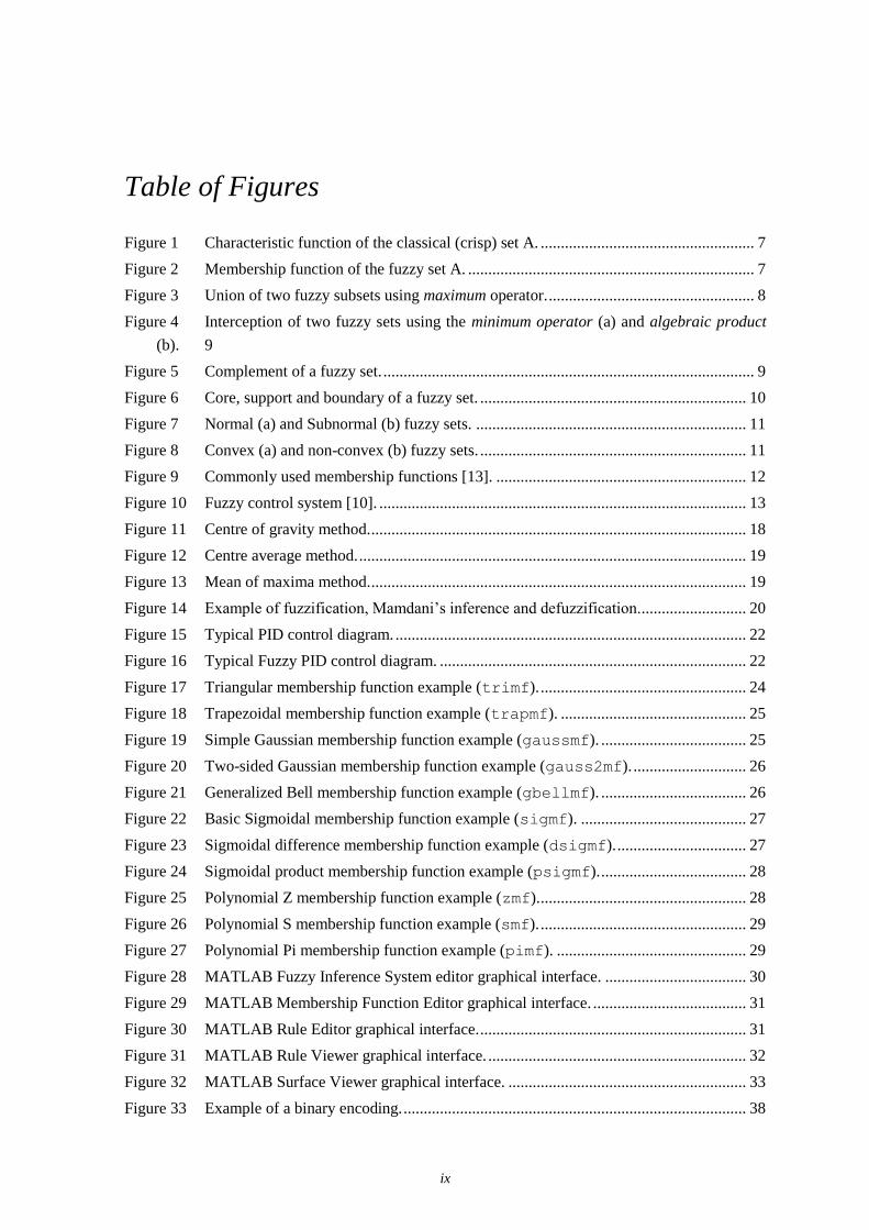
The functions are [18]:

Triangular

The triangular membership function is one of simplest ones and the name in the toolbox is

trimf. This function is nothing more than a collection of three points forming a triangle

(Figure 17).

Figure 17 Triangular membership function example (trimf).

25

Trapezoidal

The trapezoidal membership function, the trapmf, has a flat top and really is just a

truncated triangle curve (Figure 18).

Figure 18 Trapezoidal membership function example (trapmf).

Simple Gaussian

The simple Gaussian membership function, the gaussmf (Figure 19).

Figure 19 Simple Gaussian membership function example (gaussmf).

26

Two-sided Gaussian

The two-sided composite of two different Gaussian curves, the gauss2mf (Figure 20).

Figure 20 Two-sided Gaussian membership function example (gauss2mf).

Generalized Bell

The generalized bell membership function is specified by three parameters and has the

function name gbellmf. The bell membership function has one more parameter than the

Gaussian membership function, so it can approach a non-fuzzy set if the free parameter is

tuned (Figure 21).

Figure 21 Generalized Bell membership function example (gbellmf).

27

Basic Sigmoidal

Sigmoidal membership function, which is either open left or right, and the name is sigmf

(Figure 22).

Figure 22 Basic Sigmoidal membership function example (sigmf).

Sigmoidal Difference

The sigmoidal difference membership function is the difference of two membership

functions, and the name is dsigmf (Figure 23).

Figure 23 Sigmoidal difference membership function example (dsigmf).

28

Sigmoidal Product

The sigmoidal product membership function is the product of two membership functions,

and the name is psigmf (Figure 24).

Figure 24 Sigmoidal product membership function example (psigmf).

Polynomial Z

Polynomial Z membership function is based on the Z function curve, the asymmetrical

polynomial curve open to the left, and the name is zmf (Figure 25).

Figure 25 Polynomial Z membership function example (zmf).

29

Polynomial S

Polynomial S membership function is based on the S function curve, is the mirror-image

function that opens to the right and the name is smf (Figure 26).

Figure 26 Polynomial S membership function example (smf).

Polynomial Pi

Polynomial Pi membership function is based on the Pi function curve, is zero on both

extremes with a rise in the middle and the name is pimf (Figure 27).

Figure 27 Polynomial Pi membership function example (pimf).

30

The Fuzzy Inference System (FIS) editor of the toolbox can be opened typing the

command fuzzy in the MATLAB command line. With this the editor opens with default

values. The graphical interface of the FIS editor looks like the diagram shown in Figure 28.

Figure 28 MATLAB Fuzzy Inference System editor graphical interface.

The default inference mechanism is the Mamdani’s inference mechanism, which will be

the one used in this work. The FIS editor allows to change the logic operations of rules,

implication, aggregation and defuzzification method. It also permits adding inputs and

outputs, likewise the membership functions and its range.

The Membership Function Editor is the tool used to display and edit the membership

functions associated to every input and output for the entire inference mechanism. Figure

29 shows the graphical interface of the Membership Function Editor. This interface allow

users to add and edit membership functions for every input and output, as its limit ranges.

In this interface is possible to choose between the membership functions available from the

toolbox, or user defined functions, and edit its parameters, add membership functions for

every variable and edit the range of the universe of discourse for that all variables. These

configurations must be done for all variables independently.

31

Figure 29 MATLAB Membership Function Editor graphical interface.

Another tool that is also available is the Rule Editor that is represented in Figure 30. This

graphical tool allow users to add rules to the rule-base. In this interface the user can create

the rule-base based on the inputs and outputs and their relations. These relations are logic

operations, the antecedents, that imply a certain consequents to the outputs. The logical

operations are the AND, the OR and the NOT. Is also possible to define a weight for every

rule.

Figure 30 MATLAB Rule Editor graphical interface.

32

The Rule Viewer is another graphical interface that displays a roadmap of the whole fuzzy

inference process. This interface represent the antecedents and consequents of the rules

according to the implications and aggregation operands used. Here is possible to see how a

change in the inputs affects the outputs according to the defuzzification function selected

in the FIS interface. This Rule Viewer interface is shown in Figure 31.

Figure 31 MATLAB Rule Viewer graphical interface.

The Surface Viewer is used to show the entire span of the output set based on the entire

span of the input set. The surface can be either 2D or 3D based on number of inputs and

outputs. A 2D surface needs two variables and a 3D surface need 3 variables, two inputs

and one output, however, if the system has more than two inputs and more than one output,

it is not possible to show a surface for all because the surface is a 3D space, only three

variable are possible, thus, several surfaces are created and each one appears by selecting

two inputs and one output only. The surfaces can be more or less smooth, depending on the

number of plot points, that can be edited in the interface. The interface is shown in Figure

32.

33

Figure 32 MATLAB Surface Viewer graphical interface.

With all this in mind, is now possible to export the project to the MATLAB workspace or

to a file, where all this fuzzy logic parameters will be saved to later be used as a fuzzy

logic block. This block can also be imported to the SIMULINK software and be used in

simulation projects to test the behaviour of the controller. In this particular case the

simulation diagram will be similar to the one shown in Figure 16, that later will be

combined with the GAs.

35

3. GENETIC ALGORITHMS

Genetic Algorithms (GAs) are techniques used for searching minimums or maximums and

for finding the solutions that satisfy the objectives of the problem. When solving a problem

with GAs the best solutions are found after a few interactions or generations, where

crossover and mutations happen until the best individuals, that satisfy the requisites of the

problem in question, are found. These objectives are fulfilled in an evolutionary way

performing operations in the codified structure, the chromosome, resembling what happens

in nature.

GAs where developed by John Holland and his colleagues and students in the University of

Michigan during the 60’s and 70’s [9]. In contrast to other evolutionary strategies and

programming, the main goal of Holland, was not to develop algorithms to solve scientific

problems, but to study the phenomenon of adaptation as it happens in nature, by

developing ways to import these natural mechanisms to computational systems. In his

book Adaptation in Natural and Artificial Systems (1975) he showed GA as an

interpretation and adaptation of what happens in nature [9][19].

Charles Darwin’s Theory of Natural Selection is the base to better understand the evolution

of GAs. According to this theory, in one population of individuals, only survive and

reproduce the most able individuals; the less able ones die eventually after some

36

generations. Charles Darwin observed with different evolutionary characteristics in birds

of the same species, in different Galapago’s islands. As an example, he observed birds

from the same species with different nozzles shape, as an attempt of a better adaptation to

the habitat they were in. This adaption is the result of several generations that were high

lightening the expression of the advantage of that characteristic to easily find food.

Darwin’s theory was very contested for not totally answering how this individuals diversity

or their characteristics are passed over future generations.

In the XX century, with the discovery of genetic material, genetics started to answer these

questions. All living organisms are composed of cells; the cells are then composed of

genes that have on its structure a combination of basic units named DNA

(deoxyribonucleic Acid). These small units are responsible for setting the characteristics of

each individual. These sequences and combinations of genes are denominated

chromosomes, where the genetic information is stored. Even with low probability, crossing

over might cause mutations that can lead to individuals with characteristics more or less

competitive in the environment they are in. However, these mutations may result in non

significant impact to the individual. Concepts such as chromosome, gene, crossover,

mutation, fitness function, population or generation are present in GAs.

The word genetics comes from the word gene. Genetics is the science that studies the

transmission of hereditary characteristics from one generation to another. All the biological

information is codified in genes that are the basic units of a chromosome. These specific

characteristics can be genotypic (allelic constitution) or phenotypic (observable

characteristic of appearance or physiology). The same gene may have alternative forms

called alleles, which means that an allelic variation causes hereditary variation within a

species. The chromosome region where a gene is located is called locus (plural, loci).

During replication, which is the crossing over of genetic material between two individuals,

the molecular information of the progenitors is carried out to the next generation. Although

rare sometimes mutations may occur [20]. In fact, a mutation can contribute for genetic

variability within a species. The individual’s characteristics combined with the

environmental conditions determine the basis of natural selection process of species, where

the strongest ones are always selected. So, the relative probability of survival and

reproduction rate of a phenotype or genotype is called Darwinian fitness, which evaluates

37

the ability of each individual to survive and reproduce [20]. All this genetic concepts are

present in GAs as their biological basis.

In GAs, the chromosome normally represents an individual and a possible solution to the

problem, commonly encoded as a string of bits, since computer memory is composed by

matrices of bits; in fact, any information can be codified by a sequence of bits. The genes

are either single bits or short blocks of adjacent bits that encode for a particular element of

the chromosome or for a possible solution. An allele in a bit string is typically a 0 or a 1,

depending on the terminology used to represent it. At each locus more alleles are possible

when using larger alphabets. Crossover typically consists of exchanging genetic material

between two single parent’s chromosomes. Mutation consists of inverting the bit at a

randomly chosen locus (or, for larger alphabets, replacing a symbol at a randomly chosen

locus with a randomly chosen new symbol). The majority of genetic algorithms

applications use single chromosome individuals, i.e., haploid individuals. Considering a

GA using bit strings, the individual genotype is simply the configuration, of that

individual’s chromosome, in bits [9]. An analogy between genetics and genetic algorithms

is displayed in Table 3.

Table 3 Correspondence between genetics and genetic algorithms concepts.

Genetics Genetic Algorithms

Chromosome Vector or string

Gene Characteristic

Allele Value of the characteristic

Locus Position in the vector

Genotype Structure or codified vector

Phenotype Set of parameters, decoded structure

38

3.1. TYPES OF ENCODING

Encoding is the process of representing the individual genes, using bits, numbers, trees,

matrices, lists or other objects that better represent the individual that will depend on the

problem itself. Regarding the searching and learning method, the way how candidate

solutions are encoded is a central factor for the success of a genetic algorithm. Most GA

applications use fixed length, i.e., a fixed order of bit strings to encode candidate solutions.

However, recently, many experiments have been performed with other types of encodings.

The decision on the most appropriate encoding technique must be taken by the developer.

In fact, the developer needs to do the trial, test for errors and adapt the encoding that better

fits the problem. One interesting idea is to have a self-adaptable encoding so that the GA

could make better use of it [9][21].

The binary encoding is one of the most common forms of GAs encoding. Nevertheless, for

many applications it is common to use an alphabet with many characters or real numbers to

represent chromosomes. These types of encoding forms uses specific approaches by

applying encoding characters such as octal, hexadecimal, real numbers permutation,

values, or tree [9].

3.1.1. BINARY ENCODING

In binary encoding each chromosome codifies one binary string and each bit in the

sequence represents one characteristic of the solution. Despite that, this string might also

represent an integer or real number. Binary encoding varies with problems and allows

chromosomes with less number of alleles. According to Holland (1975) [19], binary

encoding has the advantage of using less space to store the same data which could result in

a better performance. Nevertheless, this type of encoding is not natural to many problems

and, sometimes, several modifications must be done after the genetic operations. The most

commonly used binary string is the encoded with zeros and ones where the length of the

string depends on the required precision. The encoding shown in Figure 33 is an example

of binary encoding.

Figure 33 Example of a binary encoding.

39

3.1.2. MANY-CHARACTER AND REAL-VALUED ENCODINGS

The octal encoding is another possible form of encoding that uses octal numbers (0 to 7).

In Figure 34 it is possible to observe an example of an octal encoding.

Figure 34 Example of an octal encoding.

The hexadecimal encoding, represented in Figure 35, is characterized by the application of

decimal numbers (0 to 9) and letters (A to F).

Figure 35 Example of a hexadecimal encoding.

The real numbers permutation encoding is useful for ordering problems. Here, each

chromosome represents a sequence of real numbers that sometimes has to be modified

after the genetic operations so that the consistency of the chromosome is kept and,

therefore maintained the sequence validity. The encoding represented in Figure 36 is an

example of real numbers permutation encoding.

Figure 36 Example of real numbers permutation encoding.

The value encoding is also another form of encoding that consists in a sequence of values

that can be anything related with the problem, such as real numbers, characters or other

type of objects. Considering an event where complicated values, such as real numbers, are

used the application of binary encoding would be very difficult; in this case, the value

encoding leads to better results. But sometimes the development of new genetic operators,

specific for the problem, is required. In Figure 37 an example of a value encoding is

displayed.

40

Figure 37 Example of a value encoding.

3.1.3. TREE ENCODING

The tree encoding is another encoding possibility considering genetic programming

evolution. In this case, each chromosome is a tree of some objects such as functions and

commands in a programming language. One advantage of tree encoding is the searching of

open-ended spaces, although there is the risk of uncontrolled tree growing where many of

these very large structured trees might difficult reading.

3.2. GENETIC ALGORITHMS

An algorithm is a sequence of steps that lastly will solve a problem. It is a genetic model

inspired method based on searching and finding the best possible solutions. The GA is

used to find optimal solutions in a certain search space that is the space where all possible

solutions are present, and where each point of the search space represents a possible

solution. The distance between two sequences of candidate solutions is the number of

positions in which the bits, at the corresponding positions, differ from each other. In most

cases the next candidate solutions will depend on the previous test sequencing results.

Some algorithms assume the existence of some correlation between the quality of the

neighbouring candidate solutions. Genetic algorithms assume that high quality parent

candidate solutions, from different regions in the space, can be combined via crossover to

produce high quality offspring candidate solutions [9].

In GA the populations of chromosomes are processed by successively replacing one

population for another. Here, the fitness function is a key concept that, in the current

population, gives a score (fitness) to each chromosome in order to evaluate how that

chromosome solves the problem. The greater the fitness function the higher the probability

of an individual being selected for reproduction and remain alive [9]. Therefore, the main

objective of this technique is to find the best solutions in all space. However, one of the

problems in searching and finding these solutions is the presence of local optimal solutions

and the selection of the starting point of search; local optimal solution might not be the

global optimal solution leading to bad solutions. Since these types of algorithms are

41

stochastic, even if the search space has no optimal local there is no guarantee that the GA

will find the global optimal solution, but instead a reasonable good solution, i.e., the

solution that satisfies the problem specifications [9].

In simple GA operators such as crossover, mutation and selection are used. Moreover,

inversion, gene doubling or deletion are also applied operators. So, the selection of the

most appropriate operator depends on the problem as well as on the GA developer.

3.3. DESIGNING GENETIC ALGORITHM PRINCIPLES

Before implementing a GA it is important to understand some guidelines in order to create

a general search algorithm, i.e., an algorithm of global optimization based on the fitness

function properties and on the most common optimization methods.

A purely deterministic search may lead to an extremely high quality solution. A non

deterministic search should be stochastic, though it could have a substantial part of

determinism. A purely stochastic method normally is too slow, and is reasonable more

efficient deterministic predictions in the most promissory directions.

When approaching GA the criterion of integrity is very important. Every solution must

have its own codification, the non redundancy, codes and solutions should have an

univocal matching named robustness. Every genetic code produced by genetic operators

should have a matching solution, and considering the perseverance of the characteristics

the descendents must inherit useful parent characteristics. The basic steps to solve a GA

problem are the representations of the problem, the calculation of the fitness function, the

several variables and parameters involved in the control of the algorithm − population size,

crossover rate, and mutation rate − the representation of the results and the way how to

finish the algorithm.

3.4. SIMPLE GENETIC ALGORITHM

The basic structure of a GA starts with randomly generating an initial population of

individuals that might be possible solutions. Sometimes heuristic knowledge could also be

used to create the first population. This first population should be large and diverse to

explore all searching spaces, otherwise the algorithm might only explore a small part of the

search space and miss a global optimum leading to premature convergence. However, if

42

the size of the initial population is very large the computational complexity increases

taking more time to the algorithm to converge. The algorithm converges when the

individuals are so similar that a mutation might be needed to improve the population.

Every individual must be evaluated by the fitness function. The next step is to create a new

generation of individuals, using the genetic operator selection, crossover and mutation, and

repeat it until the new generation is created. The new population should then replace the

previous one. This new generation must be evaluated to see if it satisfies the requisites of

the problem. In a positive case, the algorithm stops and the solutions are found; otherwise,

the algorithm should be restarted with the last population of individuals. In Figure 38 it is

represented an example of a flowchart of a simple GA.

Figure 38 Example of a simple Genetic Algorithm flowchart.

43

Based on the previously analysed references the main tasks of a genetic algorithm can be:

- The selection of individuals for reproduction is the first step. It is a random

selection with a certain probability depending on the relative aptitude of the

individuals and where the bests are selected for reproduction. The fitness function

has an important task in the selection of individuals, in which the better values lead

to better individuals.

- The crossover is the second step of when building an algorithm. The descendents

are created by the individuals that were selected for reproduction. A combination of

two chromosomes where subparts of each other are combined, originating two new

generation chromosomes. It is important to mention that recombination and

mutation can be used to generate new individuals [9][22].

- The mutation that is a rare random change of an individual’s portion of genetic

material. This occurs after the crossover phase due to swap or inversion of one or

more genes in the generated chromosome. In every generation the reproduction

chromosomes are selected in order to originate new chromosome generations.

- The replacement is the last step where the last population is replaced by the new

generation of individuals or chromosomes. The individuals are evaluated according

to their fitness and normally the ones with high values of fitness function are the

best solutions and the better candidates to be in the new generation.

The algorithm stops when the stopping criteria is settled, i.e., when the solutions found

converge to the global optimal solution according to the specifications of the problem and

the stopping conditions.

3.5. SELECTION METHODS

The selection is the artificial mechanism of natural selection when finding the most able

individuals giving emphasis to the most able ones. This process starts a random selection

of the parent’s chromosomes in agreement with the fitness function of the individuals.

During the pressure selection, which is the ratio between the maximum aptitude and the

average aptitude, it is important to select the best individuals. If the pressure is high the

intensification grows and the better individuals are favoured; in the case of less pressure

44

the diversity will be less. The pressure leads the algorithm to improve the aptitude along

with generations. The rate of convergence of the GA is highly determined by the

magnitude of the pressure that may lead to higher rates of convergence. GAs should be

capable of identifying optimal solutions, or at least closer to the optimum, by using an

intelligent scheme of pressures. However, if the pressure is too low the rate of convergence

will be too slow and therefore the GA will take more time to find the ideal solution. On the

other hand, if the pressure is too high a premature convergence can lead to a local optimal

solution or even bad solutions [9].

Besides providing pressure selection the selection schemes should also preserve the

population diversity by helping to avoid premature convergence. In the complete absence

of pressure GA will become a total stochastic process of random walk type rendering the

selection probability equal for all individuals.

Normally there are two types of selection − the proportional and the ordinal selection.

In proportional selection individuals are selected based on the comparison of the fitness

function values with the fitness function values of other individuals. In the ordinal

selection individuals are selected based on their positions in the population rather than on

the value of their fitness function. For that, the pressure needs to be independent from the

distribution of the population fitness and only dependent on the population ranking. It is

also possible to use a scale function to redistribute the fitness population interval to adjust

the pressure. The selection has to be balanced with the variation of crossover and mutation.

A very strong selection will lead to suboptimal highly able individuals reducing the

diversity needed for evolution and progress. A very weak selection will result in a slow

evolution.

3.5.1. PROPORTIONAL SELECTION

The proportional selection or roulette wheel is a selection directly proportional to the

fitness function. Considering a circle divided by n regions, that is the size of the

population, where the area of each region is proportional to the fitness of the individual. A

roulette is placed with n cursors equally spaced; after one turn the cursors position

indicates the selected individuals. The individuals with greater area will have higher

probability of being selected more often (Figure 39).

45

This type of selection adds the sum of the fitness values for all individuals in the

population T. Then generates a random number (r) in the interval [0, T] and travels all the

population by adding the values of the fitness until the sum is equal or greater than r. The

individual whose fitness value passes that limit is the selected one. The first step is only

performed once for each population. In this case premature convergence might occur.

Figure 39 Example of a roulette wheel selection method [23].

3.5.2. RANDOM SELECTION

The selection is a method that, as the name indicates, randomly selects one of the parents

from the population. Overall, it is more appropriate to break the genetic codes than the

roulette selection.

3.5.3. RANK SELECTION

The rank selection exists due to the big differences between fitness values in the roulette

selection. First the rank selection classifies the population and then gives each individual a

fitness value determined by its classification. The worst individual will have a fitness of 1,

the second worst 2, etc. so that the best will have their fitness equal to the number of

individuals in the population. After this process all individuals have a probability of being

selected; however, this method may result in a lower convergence since the best

individuals cannot be distinguished from each other. This method reduces the premature

convergence giving more importance to the less able.

46

3.5.4. TOURNAMENT SELECTION

The tournament selection creates a selection strategy capable of adjusting the selective

pressure by applying a competition by tournament between all individuals of the

population. The tournament best individual has the highest fitness and, therefore is the

winner. The competitors and winner are placed in the matting pool to repeat the

tournament until all reproducers are selected. Further, the group of selected reproducers

has an average fitness function higher than the rest of the population. In fact, this fitness

function difference introduces the selection pressure needed to improve the next

generations in terms of fitness. Thus this method reveals to be more efficient and leads to

an optimal solution.

3.5.5. STOCHASTIC SAMPLING SELECTION

The stochastic sampling selection method is done by mapping all individuals into

contiguous segments of a line. The size of each segment is proportional to the value of the

mapped individual fitness. The sizes are normalized and a number between and

is

randomly selected, pointers are pointed to the lines segments at positions

. The individuals that own that pointed line segment are then selected. This

ensures that the selection of descendents is closer to the deserved in comparison with the

roulette selection.

3.6. CROSSOVER

The crossover step is inspired on the biological mechanisms of reproduction where living

organism from the same specie mate and give origin to new identical organisms. Crossover

is the operator responsible for the recombination of the parent’s characteristics during

reproduction leading to the inheritance of these features by the new generation. It is

considered the most predominant genetic operator, so it is applied with the probability

given by the rate of crossing. To achieve this purpose some crossover techniques can be

used:

- One point crossover. A point of crossing is randomly selected and in that point the

genetic information is switched. One part of each parent is given to the child so that

it will keep the same chromosome format as parents.

47

- Two points crossover. Based on the same principle as the one point crossover, but

instead of switching the information of both parents in two parts, it switches the

information in three parts. The child receives two parts from one parent and one

part of the chromosome of the other parent.

- Multi-point crossover. It is a generalization of one point crossover where several

points are chosen to transfer the information to the child, keeping the same

principle as the one and the two point crossover.

- Uniform crossover. In this case points are not used; instead a probability for each

variable is applied to be changed by parents to the child using an auxiliary

chromosome as a mask that determines the probability.

- The three parents crossover technique compares each bit of the first parent with the

second parent and if they are equal the bit passes to the child; if not the bit of the

third parent is passed instead.

- The reduced surrogate crossover constrains the crossing to insure the creation of

new individuals when possible. The implementation is made constraining the

crossing to the points where the gene’s values are different.

- The shuffle selection is related with the uniform crossing. One crossing point is

used, but before switching the variables they are randomly disordered in both

parents; after recombination the variables are reordered.

- The precedent preservative crossover (PPX) keeps the order of the parent’s gene

precedence throughout a mask similar to the mask used in the uniform crossing.

This method selects genes from one parent; in case this gene creates a non-viable

child the operator searches for the next gene of the same parent to maintain the

child viability.

- In the partially mapped crossover (PMX) two randomly crossing points are made in

both parents; the resulting subchains genes are integrally inherited by both children.

These subchains also determine the relationship mapping between the parent genes

with the goal of treating the infeasibility originated by the process.

48

- The ordered crossover (OX) is based on the idea that, two randomly crossing points

are made in both parents and the resulting gene subchains are inherited integrally

by both children. After the last cut in each chromosome, other parent’s genes that

are not in the inherited subchain, are then searched to fill the child chromosome.

The frequency at which the crossover is done is called crossover probability. If there is no

crossing the children are exact copies of their parents. But if crossing occurs the children

chromosomes are a mixed of their parent’s chromosomes parts. If the probability of

crossover is 100%, then all children chromosomes are created by the crossing. A high

crossing probability means that new structures are rapidly introduced in the population; if

this rate is too high structures with high fitness could be removed and the greater part of

the populations will be replaced. If this rate is low the algorithm could become too slow.

3.7. MUTATION

Mutations happen at a very low probability and consist of small changes during the

crossing over of the genetic material. These changes may occur in one or more alleles,

according to a previously settled probability.

When vectors suffer a low probability mutation algorithm may not stay blocked in an

optimal local; this will helps to recover the lost genetic materials acting as an insurance

preventing the lost of irreversible genetic material. This is traditionally considered a simple

search operator. Crossing finds the best individuals for exploring the actual solution while

mutation has the ability to explore the entire search space which is very important to keep

the population’s genetic diversity. The random insertion of new genetic structures in the

population modifies some of their constructive blocks.

There are different ways in which a mutation may occur. In binary representation a simple

mutation may consist in inverting the value of a gene with low probability. Normally the

probability is in the form of

where is the length of the chromosome. It is also possible

to implement operators of hill-climbing type, i.e., operators that only make the mutation if

the quality of the solution improves. This operator may accelerate the search, yet this must

be done with careful since the diversity of the population may be reduced leading the

algorithm to converge prematurely to an optimum local. Mutation of one bit consists in

inverting one bit from 0 to 1 or the other way around. The different types of mutations are:

49

- Mutation by change. Changes all bits from 1 to 0 and from 0 to 1 based on a mask

chromosome.

- Mutation by interchange. Two positions are randomly generated and the

correspondent bits are swapped.

- Mutation by inversion. In this case a position in the chromosome is randomly

chosen and the bits next to that position are inverted.

- Mutation by probability. The transformation of the chromosome parts is decided by

the operator. If the mutation does not take place the result is generated immediately

after crossing without any changes. If the mutation takes place, one or more parts of

the chromosome are changed. If probability is 100% the entire chromosome is

changed; on the other hand, if probability is 0% no changes are made to the

chromosome. Mutation normally prevents the algorithm to fall in local optimums.

If the mutation frequency is high the genetic algorithm becomes a random search

algorithm.

3.8. REPLACEMENT

The replacement is the last step of the entire reproduction cycle.

Two parents are removed from a fixed size population generating two children and only

two, of these four members, will pass to the new population. A method must be applied in

order to choose which individuals should stay in the new population. The technique must

proportionally influence the convergence to the selection operator. There are several

techniques for replacing the population in the genetic algorithm:

- The generation type consists in the creation of N children from one population of N

size to create the new generation that will replace all parents from the old

generation. This type of generation implies that an individual can only cross with

individuals from the same generation. Other forms of this type of generation are

and . Here from one population

of parents size are created children where . The best individuals from

both populations, parents and children, will create the next generation.

50

- The stationary type is very radical and consists in inserting new created individuals

in the population, contrary to generation actualization where all generation is

created in every generation. The insertion of a new individual normally demands

the replacement of other member of the population; in this case can be the worst or

the oldest member inserting more pressure. Normally the stationary type

actualizations use a method based in order, both for selection and replacement.

- The random replacement is other method that consists in randomly selecting two

individuals in the population and replacing them by new individuals. This

technique may be useful to keep the search in small populations since that weak

individuals may be introduced in the population.

- The weak parents replacement happens when a weak parent is replaced by a

stronger child. From the four individuals, parents and children, only the two more

able ones pass to the new population. This process improves the fitness function of

the population when used together with a selection method that uses strong parents

and weak parents for reproduction.

- The both parents replacement is a simple replacement method where the child

replaces the parents, so the parents only reproduce once, resulting in a continuous

process of moving the genetic material along with generations. However, problems

may occur if combined with a selection technique that strongly favours strong

parents. In this case, good solutions evolve but are eliminated immediately.

3.9. STOPPING CRITERIA

The algorithm stops when the defined objectives are reached. The stop criteria are:

- The maximum number of generations. If the number of generation hits the

maximum number of generations the algorithm stops.

- The time limit. If the elapsed time reaches the maximum specified time the

algorithm stops.

- The fitness limit. The fitness of the best individual, in the actual population, is less

or equal to the fitness limit the algorithm stops.

51

- The generation stall. If in a number of generations the fitness function does not

improve the algorithm stops.

- The time stall. If in a defined elapsed time the fitness function does not improve the

algorithm stops.

3.10. RESTRICTIONS

To apply the GA to a real and practical problem it is necessary to deal with some

restrictions such as financial ones, rules that cannot be broken or market dynamics.

Scientific problems may also be subjected to some restrictions such as numeric ones,

temperature, light or even time.

Essentially there are two types of restrictions, the hardconstrains and the softconstrains.

The hardconstrains are restrictions that must be completely followed otherwise the solution

will not be valid. The softconstrains are desired but may not be followed, for instance

speed is always positive and in this case the search space is all positive numbers so there is

no need to search negative numbers, leading to a faster algorithm.

The search space is always divided in two regions, the feasible and the non-feasible region.

The feasible region is the part of the search space where the solutions satisfies the

restrictions, the rest corresponds to the non-feasible region. Although, invalid solutions

should not be completely removed from the search space, thus they may be near an optimal

solution as represented in Figure 40.

Figure 40 Example of search space with restrictions and feasible region.

52

3.11. MATLAB GLOBAL OPTIMIZATION TOOLBOX

As previously mentioned, MATLAB is a mathematical computation tool used to develop

and simulate numerous scientific and engineering problems. It contains the Fuzzy Logic

Toolbox plus the Global Optimization Toolbox (GOT) to work with GAs. This toolbox is a

collection of functions that includes routines that allows solving optimization problems by

using GAs. Those functions are the ga, the gaoptimset and the gaoptimget [24].

The MATLAB version used for this work was the R2011b and the Global Optimization

Toolbox was version 6.1.

To solve a minimization or maximization problem using this toolbox it is necessary to

define the problem’s fitness function to then minimize or maximize. The toolbox itself

does not applies the maximization, but instead solves the problem by using the form:

So if the intention is to maximize it can be done by minimizing .

First of all, it is important to mention that the images displayed in this section result from

the application and manipulation of the MATLAB toolbox software [24]. Overall, there are

two different ways to start the GA toolbox, i.e., this can be done by using the command

line or by means of a graphical interface. To use the GA from the command line, the basic

syntax presented below must be written, allowing the call of the ga function displayed:

[x fval] = ga(@fitnessfun, nvars, options)

Where:

@fitnessfun is a handle to the fitness function.

nvars is the number of independent variables for that fitness function.

options is a structure that contains options for the genetic algorithm. In case this

argument does not pass the default options will be assumed.

Then the results are stored in:

fval is the final value of the fitness function.

53

x is the point at which the final value is attained.

The function gaoptimset is used to set the options parameters in the genetic algorithm.

It is used to set parameters such as population size, restrictions, limits, operators, stopping

criteria and the remaining used in genetic algorithms. Once the options are set, it is

possible to see the selected ones that will be used by the ga function. To do that it is

required to use the gaoptimget function.

Despite the previously mentioned, to obtain more information regarding the several ga

function options it is important to analyse the user’s manual or to use the command line

typing ’help ga’.

In case the user wants to use the GA with the graphical interface, and without using the

command line, the syntax optimtool (‘ga’) − that opens the window shown below

(Figure 41) − must be entered.

54

Figure 41 Genetic algorithm solver graphical interface.

55

4. OPTIMAL TUNING OF

FUZZY PID CONTROLLERS

This chapter presents the simulation results for the Fuzzy Logic PID controller tuned with

GAs (FL-PID). Simulations were also performed for the PID controller tuned with ZN

step-response method (PID-ZN) and for the PID controller tuned with GAs method (PID-

GA). In addition to these tuning methods, an optimal tuning method named Zhuang

Atherton (ZA) setpoint method was also applied for comparison purposes. The mentioned

controllers were tested with six benchmark systems with different dynamics and

characteristics.

The main purpose of this work is to develop a FL-PID controller that uses GAs to achieve

the parameters optimization, and thus reducing the system step response error to a

minimum. For that, several performance indices were adopted in the simulations.

Moreover, the step responses and the performance indices results were compared in order

to evaluate the effectiveness of the GAs in tuning the PID and Fuzzy PID controllers.

4.1. BENCHMARK SYSTEMS

The proposed Fuzzy controller intends to be used for controlling several types of systems

without the need of changing the controller itself, but only their parameters in order to

56

control that particular system. These parameters should then be tuned with GAs to find the

optimal values.

The FL-PID controller must be compared with other type of control to evaluate its

performance. The chosen controller used for comparison purposes was the classical PID

controller. To compare both controllers’ performances, six benchmark systems with

distinct characteristics are proposed:

System 1: First order system with delay [25]:

(28)

System 2: Fast and slow mode system [26]:

(29)

System 3: Fourth order system [26]:

(30)

System 4: Fourth order system with three zeros [25]:

(31)

System 5: Inverted pendulum system [27]:

(32)

System 6: Time varying system with the following differential equation [28]:

(33)

The systems were controlled using both types of control (PID and FL-PID). Firstly,

systems were controlled with PID-ZN and PID controller tuned with Zhuang and Atherton

method (PID-ZA). It is important to mention that these methods cannot be used for

systems 5 and 6 since they cannot be approximately modelled by a first order plus time

delay (FOPDT) model. Later, systems were controlled using PID-GA and FL-PID

controllers.

57

To approach the simulation to a real control system, a non-linearity was implemented on

the controller output. The saturation levels were set equal for both PID and FL-PID

controllers, so they can be compared with each other.

4.2. PERFORMANCE INDICES

The error measurement allows the evaluation on how the system tuning is being evaluated.

If the tuning is correctly performed, the error is low; however, if the tuning is poor, the

error value is higher. Bearing this in mind, and considering the system response, the

performance indices can be achieved by measuring the system step response error.

There are several performance indices errors [29]. Nevertheless, the work focus on four,

namely the Integral of Absolute Error (IAE), the Integral of Square of the Error (ISE), the

Integral Time multiplied by the Absolute Error (ITAE) and the Integral of Time multiplied

by the Square Error (ITSE).

The IAE criterion measures the absolute error deviation from the reference along the time

and the mathematical expression is as follows [4]:

(34)

The main disadvantage of the ISE criterion is that it amplifies large errors and

consequently, leads to closed-loop oscillation. The mathematical representation is as

follows [4]:

(35)

To minimize the initial error impact of the step response, and to amplify the error in

steady-state the ITAE was also used. This performance index is the one that provides the

best selectivity and whose mathematical expression is [4][29]:

(36)

The other used criterion was the ITSE, similar to the ITAE criterion, whose mathematical

expression is [29]:

58

(37)

In all performance indices expressions the parameter is the simulation time and

is the error, as the difference between the reference signal (step) and the output response.

4.3. PID CONTROLLER

The controller used to compare with the FL-PID was the classical PID and the SIMULINK

diagram used was a simple PID with a low-pass filter on the derivative part, without

disturbances for simplicity purposes (Figure 42). To simulate a real control system, a

saturation was implemented after the controller which expression is as follows:

(38)

This model accepts gains ( ) as inputs for the PID block in accordance to ZN, ZA

or GA methods and returns IAE, ISE, ITAE and ITSE performance indices.

Figure 42 Block diagram of the PID control system.

4

ITSE

3

ITAE

2

ISE

1

IAE

G(s)

SystemStep ScopeSaturation

Product1

Product

PID(s)

PID Controller

|u|2

Math

Function1

|u|2

Math

Function

1

s

Integrator4

1

s

Integrator3

1

s

Integrator2

1

s

Integrator1

Clock1

|u|

Abs1

|u|

Abs

59

As previously shown, the expression of a classical PID controller can be given as:

(39)

or

(40)

Where:

(41)

(42)

(43)

The parameters and are the proportional, integral and derivative gains,

respectively. These gains are the variables subjected for tuning in the PID controller.

For practical applications, it is common to apply a first order low-pass filter in the

derivative part to reduce the noise that is produced in the derivative part [30][28]. The

transfer function of the PID with the filter in derivative part can be represented as follows:

(44)

The first order low-pass filter has a coefficient , which is normally set to if both

controllers, (40) and (44), should have similar responses. In this work we set .

To obtain the PID gains using ZN and ZA tuning methods the system should be

represented as an approximation of a FOPDT model whose transfer function is [30]:

(45)

where and are the system gain, time delay and time constant, respectively.

60

Dingyu Xue et al. (2007) [28] proposed a MATLAB function (opt_app) that identifies

the system and approximates it to a FOPDT model. The MATLAB syntax that finds the

FOPDT model parameters is shown below [28]:

Gr = opt_app(G,0,1,1);

[n,d] = tfdata(Gr,'v');

k = dcgain(Gr);

T = d(1)/d(2);

L = Gr.ioDelay;

The ZN gains calculation was done using a MATLAB function (ziegler) also

proposed by Dingyu Xue et al. (2007) [28], based on the ZN step response and frequency

response methods (Table 4). The function receives the transfer model parameters and

returns the PID parameters. The function syntax is as follows:

% ZN step response method

[Gc,Kp,Ti,Td] = ziegler(3,[k L T N])

Kp = Kp;

Ki = Kp/Ti;

Kd = Kp*Td;

Table 4 PID controller parameters obtained from the ZN methods [28].

Step response Frequency response

Control type

P

PI

PID

Where:

(46)

The parameters and given in Table 4 are obtained when the system is in the limit of

stability, i.e. oscillating, and known as the ultimate gain and the ultimate period,

respectively.

61

Table 5 PID controller parameters using ZA setpoint method [28].

Range of

Criterion ISE ITSE IST2E ISE ITSE IST

2E

1.048 1.042 0.968 1.154 1.142 1.061

-0.897 -0.897 -0.904 -0.567 -0.579 -0.583

1.195 0.987 0.977 1.047 0.919 0.892

-0.368 -0.238 -0.253 -0.220 -0.172 -0.165

0.489 0.385 0.316 0.490 0.384 0.315

0.888 0.906 0.892 0.708 0.839 0.832

To find the PID gains using the ZA tuning methods another function (optpid) was

used [28]. The PID parameters are calculated as follows:

(47)

(48)

(49)

Where for different ratio

, the coefficients are defined in Table 5.

The ZA setpoint method uses three performance indices to calculate the PID parameters,

the ISE, the ITSE and the Integral Squared Time-squared weighted Error (IST2E) [28].

However, in this work it was decided to use only the ITSE criterion. The statement syntax

to find the PID parameters is represented below:

% ZA setpoint method using ITSE criterion

[Gc kp Ti Td]= optpid(3, 1, [k L T N 2]);

Kp=kp;

Ki=kp/Ti;

Kd=kp*Td;

62

4.4. FUZZY LOGIC PID CONTROLLER

Regarding the FL-PID controller, it was used a Fuzzy Logic PD+I controller whose

diagram is represented in Figure 43 and the expression is as follows [31]:

(50)

where is a nonlinear function of inputs, error ( ) and derivative of error ( ).

To test if the FL-PID controller is properly designed it is possible to use the PID controller

gains results from the ZN method, but with the FL-PID controller linear approximation.

Then both step responses must be exactly the same [31].

The linear approximation of the fuzzy PID diagram is [31]:

(51)

(52)

Where:

63

Figure 43 Block Diagram of the Fuzzy PD+I control system.

The FL-PID controller linear approximation implies that the rules-base should act as a

summation. The input and output sets have to be triangular functions and 50% overlapped,

i.e., the sets should be crossed at , for the AND connective must be used the

algebraic product, the output of the rule base must be the AND product of all inputs and

the COG defuzzification method must be used [31]. This controller has four gains instead

of three − , , and – thus, this controller has four degrees of freedom against

three in the classical PID. The should be non-zero and must be set as the maximum

error in the fuzzy controller. The other three gains are calculated as follows:

(53)

(54)

(55)

4

ITSE

3

ITAE

2

ISE

1

IAE

Step ScopeSaturation

Product1

Product

|u|2

Math

Function1

|u|2

Math

Function

1

s

Integrator4

1

s

Integrator3

1

s

Integrator2

1

s

Integrator1

1

s

Integrator

Ku

Gain3

Kce

Gain2

Kie

Gain1

Ke

Gain

Fuzzy Logic

Controllerdu/dt

Derivative

Clock1

|u|

Abs1

|u|

Abs

system

64

The SIMULINK model presented above (Figure 43) is used for all the displayed systems

and is based on a Mandani fuzzy inference mechanism.

Seven linguistic terms were used for both inputs (error and change on error) and output and

since the terms are 7, the rules used for all the systems are 49 and are listed in Table 6.

Table 6 Fuzzy rule-base for output.

NB NM NS Z PS PM PB

NB NB NB NB NB NM NS Z

NM NB NB NB NM NS Z PS

NS NB NB NM NS Z PS PM

Z NB NM NS Z PS PM PB

PS NM NS Z PS PM PB PB

PM NS Z PS PM PB PB PB

PB Z PS PM PB PB PB PB

Before choosing the membership functions, some tests were made in order to check which

function better fits the proposed problems. Simulations, using triangular functions and

Gaussian functions, were made. The results with Gaussian functions revealed to be better

for the majority of systems. Therefore, the Gaussian membership functions were chosen

for all the linguistic variables (error, change on error and output).

In order to find the input and output membership function limits that better fit all the

proposed systems some tests were also done. The best results were achieved for the

linguistic variables limits between for both inputs and output. The distribution of the

membership functions along the universe of discourse were chosen empirically and were

set as in Figure 44. For this fuzzy inference mechanism the corresponding surface is shown

in Figure 45.

Another parameter from the Mandani inference mechanism, that was changed from its

default value, is the antecedents of rules AND method, that was set to use the product (*)

operator instead of the minimum operator. The

remaining parameters were left as default. The OR method for the antecedents rules, uses

the default maximum operator. The rules’ weight is the

same for all rules and was left as default, i.e., equal to one. The implication method of rules

65

uses the default minimum operator. The aggregation of rules uses the default maximum

operator and the defuzzification method to find the crisp output value is the default COG.

These parameters were set as displayed in Figure 46.

(a)

(b)

Figure 44 Gaussian membership functions of inputs (a) and output (b).

66

Figure 45 Output control surface.

Figure 46 Fuzzy inference system.

67

4.5. STRUCTURE OF THE GENETIC ALGORITHM

GAs were chosen to find the optimal parameters for the PID and FL-PID controllers; for

that a MATLAB program was created. This program uses the function ga available in the

MATLAB GOT [24]. The function that allows changing the ga parameters is the

gaoptimset. The changed parameters are: the number of generations, the population

initial range, the population size, the creation function, the selection function, the crossover

function, the mutation function, the tolerance function and the initial population; the

remaining parameters were left as default. To create the initial population the function

gacreationlinearfeasible was used; this is the default creation function when

there are constrains. An individual was inserted to the initial population − the resulting

gains of the ZN tuning, except for systems 5 and 6 where there are no results. The

crossover function used is the crossoverscattered, and the mutation function used

is the mutationadaptfeasible.

The stopping criterion, number of generations, was changed to 70 generations instead of

the default value of 100 generations. This number of generations was chosen because after

some tests with both numbers of generations the fitness results were very similar in all the

cases. Despite this, it is important to mention that for some cases, 30 generations are

sufficient. Overall, 100 generations do not significantly improve the fitness functions, and

the costs of processing time do not compensate the improvement. The processing time for

100 generations is approximately 30% more than the time to process 70 generations. In

fact, in some cases the algorithm started to converge far before the 70 generations. Since

the purpose of this work is to develop a FL-PID that covers the largest number of systems

possible, 70 generations seems to be a good commitment between the algorithm

performance and the systems response. Despite this stopping criterion, the algorithm

should stop after a certain number of generations, if the fitness does not improve, even if

the number of generations stopping limit is not reached. Thus, the GA option tolerance

function value for the stall generations limit was changed to 0 and the stall number of

generations was changed to 20.

The number of chromosomes are denoted as population size and defined as 30 individuals.

Initially, some tests were performed with 50 individuals but the processing time was very

high and does not justify the cost regarding the results, i.e., the fitness values were very

similar. During the first tests, the algorithm showed that it is preferable to have more

68

generations rather than more individuals. The tournament selection method used was the

selectiontournament that increases some pressure in the algorithm, since the global

optimal should be near the results of the ZN methods. This function uses four randomly

chosen individuals. Since the number of best individuals that migrate to the new generation

is two, the elite-count was set on 2 individuals. Some plots were selected to show

information such as the current best solution, the mean and current best individual, while

the algorithm is running. A summary with the GA parameters used in all simulations are

presented in Table 7.

Table 7 GA parameters used in all simulations.

PID FL-PID

Number of variables 3 4

Individuals 30

Generations limit 70

Stall generations limit 20

Tolerance function value 0

Elite-count 2

Creation function gacreationlinearfeasible

Crossover function crossoverscattered

Mutation function mutationadaptfeasible

Selection function selectiontournament

Plot functions gaplotbestf ; gaplotbestindiv

The GA options syntax is listed below:

options = gaoptimset('PlotFcns',...

{@gaplotbestf,@gaplotbestindiv},...

'SelectionFcn',@selectiontournament,...

'CreationFcn',@ gacreationlinearfeasible,...

'CrossoverFcn',@crossoverscattered,...

'MutationFcn',@mutationadaptfeasible,...

'StallGenLimit',20,...

'TolFun',0,...

'EliteCount',2,...

'Generations',70,...

'PopulationSize',30);

The lower bound for the variables is zero since the gains should be positive. The initial

population is defined for each system individually, the values differ from every system,

and these are the results of the ZN method for that particular system. The syntax examples

displayed below are from System 1; nevertheless, it is important to mention that the

procedure is the same for the remaining systems. An example of the code, that uses the ga

function to find the optimal gains for System 1 PID-GA and IAE criterion, is shown below:

69

vars=3;

options.PopInitRange=[0 0 0;15 1 40];

options.InitialPopulation=[Kp_ZN Ki_ZN Kd_ZN];

[X,FVAL] = ga(@Fit_01_IAE,vars,[],[],[],[],[0 0 0

0],[15 1 40],[],options)

Another example that uses the ga function to find the optimal gains for System 1 FL-PID

and IAE criterion is shown below:

vars=4;

Ke_ini=20;

Ku_ini=Kp_ZN/Ke_ini;

Kce_ini=Kd_ZN/Ku_ini;

Kie_ini=Ki_ZN/Ku_ini;

options.PopInitRange=[0 0 0 0;30 100 2 2];

options.InitialPopulation=[Ke_ini Kce_ini Kie_ini

Ku_ini];

[X,FVAL] = ga(@Fit_01_IAE,vars,[],[],[],[],[0 0 0

0],[30 100 2 2],[],options)

Regarding the fitness function, it receives the variables (gains) and returns the fitness value

for the current variables. According to the number of variables, 3 or 4, the function

processes the PID or the FL-PID control system, respectively. The SIMULINK model is

called and returns the four performance indexes (fitness values) calculated in the system.

An example of the fitness function code for System 1 and IAE criterion is displayed below:

function J=Fit_01_IAE(K)

if length(K) < 4

% PID-GA

Kp=K(1);

Ki=K(2);

Kd=K(3);

[T X IAE ISE ITAE ITSE]=sim('PID_Sys_01.mdl');

else

% FL-PID

Ke=K(1);

Kce=K(2);

Kie=K(3);

Ku=K(4);

[T X IAE ISE ITAE ITSE]=sim('Fuz_Sys_01.mdl');

end

J=IAE(end);

The PC used has installed the Windows7 64 bit Home Premium Service Pack 1 operating

system. The CPU is an Intel Core Duo P7450 running at 2.13 GHz with 4.00 GB of RAM.

The MATLAB version edition installed is the R2011b 64-bit and the Global Optimization

Toolbox (which includes Genetic Algorithms) is the version 6.1.

70

4.6. SIMULATION AND RESULTS

The simulation and results for the systems response controlled with PID and FL-PID

controllers are presented in this section. It is important to mention that, to have results with

statistical value, the GA was performed 10 times and the best result was selected. In the

first four systems, the PID-ZN and PID-ZA were used and compared with PID-GA and

FL-PID. As already mentioned, Systems 5 and 6 were not controlled using the PID-ZN and

PID-ZA. The system step responses are presented and the performance indices displayed in

order to compare and discuss the obtained results.

4.6.1. SYSTEM 1

System 1 uses a first order system with a delay; it was proposed by Nina et al. (2008) [25],

and its transfer function is represented as follows:

(56)

Figure 47 Step response of System 1.

The system uncontrolled step response is shown in Figure 47. According to the system

dynamics response, the step time used for the simulations was and the

simulation time was , which are reasonable values and covers the four

simulations (PID-ZN, PID-ZA, PID-GA and FL-PID). The controller output saturation

0 50 100 150 200 2500

0.1

0.2

0.3

0.4

0.5

0.6

0.7

Step Response

Time (seconds)

Am

plit

ude

71

limits were set to . The initial population and upper bounds used in the GAs are


Table 8 GA upper bounds and initial population used for System 1 simulations.

PID FUZZY PID

Initial Population 12.0295 0.8853 40.8636 20 67.9391 1.4719 0.6015

Upper Bounds 20 1 45 30 80 2 1

The GA fitness evolution, for the 70 generations, for the IAE, ISE, ITAE and ITSE criteria

for PID-GA and FL-PID controllers are shown in Figure 48. The fitness evolution of

System 1 converged (meaning that it has approximately the same fitness value of the last

generation) in all the tested criteria before the 40th

generation. It is notorious that regarding

the PID-GA, this convergence for the IAE and ISE criteria occurred right after 10

generations. In the case of the PID, and comparing both controllers, the GA required less

generations to converge the fitness to the final value.


regarding System 1.

0 10 20 30 40 50 60 7013

14

15

16

17

18

19

20

21

22

23

Generation

(a)

Fitness

PID-GA

FL-PID

0 10 20 30 40 50 60 70

10.7

10.8

10.9

11

11.1

11.2

11.3

11.4

11.5

11.6

11.7

Generation

(b)

Fitness

PID-GA

FL-PID

0 10 20 30 40 50 60 70100

150

200

250

Generation

(c)

Fitness

PID-GA

FL-PID

0 10 20 30 40 50 60 7060

65

70

75

80

85

90

95

100

Generation

(d)

Fitness

PID-GA

FL-PID

72

The obtained results for the PID-ZN, PID-ZA, PID-GA and FL-PID, such as gains,

performance indices, percent overshoot ( ), rise time ( ) and settling time ( ) are

shown in Tables 9 and 10 for the FL-PID and PID controllers, respectively.

Table 9 Results of Fuzzy PID tuned with GAs for System 1.

Criterion

Error Gains Time specifications

FL-PID

IAE 13.9626 10.4330 26.3018 0.2219 0.6219 1.2055 9.2874 20.5870

ISE 11.5351 19.9986 60.1656 0.3693 0.4788 5.1205 8.6278 >150

ITAE 166.3534 20.8174 65.8669 0.3591 0.3462 1.0232 13.4562 26.3099

ITSE 72.1393 11.6940 44.5881 0.2560 0.5957 4.8667 9.0776 123.4329

Table 10 Results of PID tuned with ZN, ZA and GAs methods for System 1.

Criterion


ZN

IAE 22.5635

12.0295 0.8853 40.8636 76.1792 6.0196 66.4432 ISE 16.1235

ITAE 391.0852

ITSE 202.4182

ZA

IAE 16.7984

8.8327 0.2719 35.4354 16.7889 6.2088 83.9584

ISE 10.9634

ITAE 311.7143

ITSE 72.4907

GA

IAE 13.3135 7.3085 0.1420 23.6208 2.6730 8.2203 35.5794

ISE 10.6158 9.8262 0.1754 36.3355 14.9986 6.0327 62.9333

ITAE 104.5882 7.8950 0.1502 25.6243 7.2207 7.1484 35.9486

ITSE 61.0970 8.7909 0.1627 31.1613 12.4503 6.4141 44.4589

The step responses of System 1 for the four controllers (PID-ZN, PID-ZA, PID-GA and

FL-PID) and for indices IAE, ISE, ITAE and ITSE are shown in Figure 49. It is possible to

state that the system step response presents worse results when controlled with the PID-ZN

controller, and is notorious the big overshoot when comparing with the other controllers. In

fact, the error was higher in all the measured criteria using this controller. The step

responses analysis showed that this controller presents the worst results, except for the rise

time, that is the best for all simulations, although, for ISE criterion the difference is not

significant when comparing with the PID-GA. The FL-PID presents the lowest overshoot

in all criteria, and the fastest settling time for IAE and ITAE criteria. The rise time of the

FL-PID is the slowest of all, but not significantly different from the other controllers,

except in the case of the ITAE criterion. In fact, this characteristic is the reason the fitness

value is not so good has the PID-GA, which has the best fitness in all criteria. The FL-PID

73

settling time for ISE and ITSE criteria is the highest observed, having an oscillation in the

steady-state. It is important to note that the ISE and ITSE criteria penalises more the initial

error than the steady-state error, and this is the reason of this oscillation for these criteria.

Overall, it is possible to state that for this system, the FL-PID presents lower overshoot for

all criteria and lower settling time in the IAE and ITAE criteria. Even though, the error

criteria are not the best, only the PID-ZN presents worse results. The PID-GA controller

presents the most satisfactory results comparing with the others PID controllers (PID-ZN

and PID-ZA).


criteria.

0 50 100 1500

0.2

0.4

0.6

0.8

1

1.2

1.4

1.6

1.8

Step response(a)

PID-ZN

PID-ZA

PID-GA

FL-PID

0 50 100 1500

0.2

0.4

0.6

0.8

1

1.2

1.4

1.6

1.8

Step response(b)

PID-ZN

PID-ZA

PID-GA

FL-PID

0 50 100 1500

0.2

0.4

0.6

0.8

1

1.2

1.4

1.6

1.8

Step response(c)

PID-ZN

PID-ZA

PID-GA

FL-PID

0 50 100 1500

0.2

0.4

0.6

0.8

1

1.2

1.4

1.6

1.8

Step response(d)

PID-ZN

PID-ZA

PID-GA

FL-PID

74

4.6.2. SYSTEM 2

System 2 uses a fast and slow mode system and was proposed by C. Thammarat et al.

(2007) [26], and the transfer function is represented as follows:

(57)


The system uncontrolled step response is shown in Figure 50. The step time used for the

simulations was and the simulation time was , which are reasonable

values and covers the four simulations (PID-ZN, PID-ZA, PID-GA and FL-PID). The

controller output saturation limits were set to . The initial population and upper

bounds used in the GAs are presented in Table 11.


PID FUZZY PID

Gains


Upper Bounds 70 5 10 40 5 60 10

The GA fitness evolution, for the 70 generations, for IAE, ISE, ITAE and ITSE criteria for

PID-GA and FL-PID controllers are shown in Figure 51. The fitness evolution of System 2

0 20 40 60 80 100 1200

2

4

6

8

10

12

Step Response

Time (seconds)

Am

plit

ude

75

converged before 10 generations for all criteria and in both controllers. The number of

generations required to converge in both controllers are similar in all cases.


regarding System 2.





Criterion


FL-PID

IAE 0.1813 28.8210 2.6536 0.7620 1.5682 2.6727 0.1551 0.6230

ISE 0.1306 26.5711 2.3094 0.9621 9.3268 1.0385 0.1481 >5

ITAE 0.0260 15.8725 1.5510 0.3868 3.0192 1.2151 0.1605 0.5693

ITSE 0.0098 20.0447 2.0265 0.5693 2.5504 2.5381 0.1508 0.5943

0 10 20 30 40 50 60 700.18

0.185

0.19

0.195

0.2

0.205

0.21

0.215

Generation

(a)

Fitness

PID-GA

FL-PID

0 10 20 30 40 50 60 700.1305

0.1306

0.1307

0.1308

0.1309

0.131

0.1311

0.1312

0.1313

Generation

(b)

Fitness

PID-GA

FL-PID

0 10 20 30 40 50 60 700.025

0.03

0.035

0.04

0.045

0.05

0.055

0.06

0.065

Generation

(c)

Fitness

PID-GA

FL-PID

0 10 20 30 40 50 60 700.0096

0.0098

0.01

0.0102

0.0104

0.0106

0.0108

Generation

(d)

Fitness

PID-GA

FL-PID

76


Criterion


ZN

IAE 0.3137

11.7007 34.1900 1.0011 54.8041 0.1377 1.0934 ISE 0.1869

ITAE 0.0982

ITSE 0.0332

ZA

IAE 0.3303

6.3133 0.4099 0.8918 0 0.3297 2.1734

ISE 0.1640

ITAE 0.2211

ITSE 0.0208

GA

IAE 0.1938 40.4850 1.1655 3.8210 4.4551 0.1484 0.9504

ISE 0.1311 39.2095 2.1186 3.4777 5.3982 0.1449 0.9861

ITAE 0.0410 42.9914 1.0016 4.6676 2.0130 0.1649 0.8765

ITSE 0.0104 49.2967 1.3481 4.6900 4.1245 0.1489 1.1165

The system step responses for the four controllers (PID-ZN, PID-ZA, PID-GA and FL-

PID) and for the indices IAE, ISE, ITAE and ITSE are shown in Figure 52. Regarding the

results for System 2, the system step responses also presents worse results when controlled

with the PID-ZN controller; in fact the error was also higher for all the measured error

criteria. The step response analysis presented worse results, except for the rise time, that

was better for all simulations. The FL-PID presents better overshoot in all simulations,

around half the overshoot of the PID-GA and PID-ZA controllers. The rise time of the four

controllers is similar, except for the PID-ZA, that is more than the double of the rise time

of the other controllers. The best results in error measurement criteria was achieved by the

FL-PID controller, despite by a small margin when comparing with the PID-GA.

Overall, it is possible to state that for this system, all controllers had similar responses,

except for the PID-ZN, that presents a big overshoot comparing with the other controllers.

Even though, with similar responses, in general the FL-PID presents better results.

77


criteria.

4.6.3. SYSTEM 3

System 3 uses a four order system and was proposed by C. Thammarat et al. (2007) [26],

and the transfer function is as follows:

(58)

0 1 2 3 4 50

0.2

0.4

0.6

0.8

1

1.2

1.4

1.6

Step response(a)

PID-ZN

PID-ZA

PID-GA

FL-PID

0 1 2 3 4 50

0.2

0.4

0.6

0.8

1

1.2

1.4

1.6

Step response(b)

PID-ZN

PID-ZA

PID-GA

FL-PID

0 1 2 3 4 50

0.2

0.4

0.6

0.8

1

1.2

1.4

1.6

Step response(c)

PID-ZN

PID-ZA

PID-GA

FL-PID

0 1 2 3 4 50

0.2

0.4

0.6

0.8

1

1.2

1.4

1.6

Step response(d)

PID-ZN

PID-ZA

PID-GA

FL-PID

78




simulation time was , which are reasonable values and covers the four simulations

(PID-ZN, PID-ZA, PID-GA and FL-PID). The controller output saturation limits were set

to . The initial population and upper bounds used in the GAs are presented in Table

14.


PID FUZZY PID

Initial Population 2.2938 1.7295 0.7605 20.000 6.6313 15.0799 0.1147

Upper Bounds 20 5 10 30 10 20 1


for PID-GA and FL-PID controllers are shown in Figure 54. In System 3, the fitness value

converged in all criteria before approximately 20 generations for both controllers. The

number of generations needed to converge are similar in all cases.

0 1 2 3 4 5 6 70

0.1

0.2

0.3

0.4

0.5

0.6

0.7

0.8

0.9

1

Step Response

Time (seconds)

Am

plit

ude

79


regarding System 3.





Criterion


FL-PID

IAE 0.7667 12.2924 5.6405 3.0024 0.4825 3.5904 0.6228 3.7046

ISE 0.5106 19.6130 9.6729 11.0075 0.5620 28.3641 0.4229 >10

ITAE 0.4619 8.7223 4.4969 2.2998 0.5709 1.9291 0.7059 2.2265

ITSE 0.1580 9.6231 4.7088 2.2796 0.7245 5.9657 0.5493 5.1601

0 10 20 30 40 50 60 700.7

0.75

0.8

0.85

0.9

0.95

Generation

(a)

Fitness

PID-GA

FL-PID

0 10 20 30 40 50 60 700.46

0.48

0.5

0.52

0.54

0.56

0.58

0.6

0.62

Generation

(b)

Fitness

PID-GA

FL-PID

0 10 20 30 40 50 60 700.4

0.5

0.6

0.7

0.8

0.9

1

Generation

(c)

Fitness

PID-GA

FL-PID

0 10 20 30 40 50 60 70

0.145

0.15

0.155

0.16

0.165

0.17

0.175

0.18

0.185

Generation

(d)

Fitness

PID-GA

FL-PID

80


Criterion


ZN

IAE 1.1330

2.2938 1.7295 0.7605 18.8131 0.8856 3.9073 ISE 0.7066

ITAE 1.1158

ITSE 0.3490

ZA

IAE 1.2170

1.8739 1.4820 0.6534 15.5804 1.0309 4.4601

ISE 0.7541

ITAE 1.3339

ITSE 0.3935

GA

IAE 0.7299 7.1659 1.5191 3.2616 4.3141 0.5533 3.3321

ISE 0.4709 9.9292 2.2709 4.4336 12.9374 0.4578 6.0390

ITAE 0.4689 6.7521 1.4556 3.1404 3.2883 0.5795 3.3448

ITSE 0.1463 7.8301 1.7342 3.4527 6.6100 0.5171 3.9531


PID) and for the indices IAE, ISE, ITAE and ITSE are shown in Figure 55. Regarding the

results of System 3, it is possible to state that the system step response presents worse

results when controlled with the PID-ZN controller; except, when compared with the

overshoot of the FL-PID (ISE criterion), and the settling time of the PID-GA (ISE and

ITSE criteria) and FL-PID (ISE criterion). The FL-PID presents lower overshoot in all

simulations, except for the ISE criterion, which presents the worst overshoot of all

controllers. The rise time has differences in all controllers but nothing significant,

nevertheless, the PID-GA and FL-PID has lower rise times than the PID-ZN and PID-ZA

controllers. In terms of settling time the differences are not notorious, except in the FL-PID

controller for criteria ISE, where the output presents an oscillatory response in steady-state.

Overall, it is possible to state that for this system the FL-PID and the PID-GA has better

results, but the differences between these two controllers are not significant, even though,

the PID-GA has slightly better responses. The other two controllers, the PID-ZN and the

PID-ZA controllers, presents worse results.

81


criteria.

4.6.4. SYSTEM 4

System 4 uses a tank with stirrer with a heating and cooling model system. It was proposed

by Nina et al. (2008) [25], and its transfer function is represented as follows:

(59)

0 2 4 6 8 100

0.2

0.4

0.6

0.8

1

1.2

1.4

Step response(a)

PID-ZN

PID-ZA

PID-GA

FL-PID

0 2 4 6 8 100

0.2

0.4

0.6

0.8

1

1.2

1.4

Step response(b)

PID-ZN

PID-ZA

PID-GA

FL-PID

0 2 4 6 8 100

0.2

0.4

0.6

0.8

1

1.2

1.4

Step response(c)

PID-ZN

PID-ZA

PID-GA

FL-PID

0 2 4 6 8 100

0.2

0.4

0.6

0.8

1

1.2

1.4

Step response(d)

PID-ZN

PID-ZA

PID-GA

FL-PID

82




simulation time was , which are reasonable values and covers the four

simulations (PID-ZN, PID-ZA, PID-GA and FL-PID). The controller output saturation

limits were set to . The initial population and upper bounds used in the GAs are



PID FUZZY PID


Upper Bounds 5 1 20 30 120 2 1


for PID-GA and FL-PID controllers are shown in Figure 57. In System 4, the fitness

converged in all criteria approximately before 30 generations, except in the PID-GA for the

IAE criterion, that required more generations, around 55.

0 20 40 60 80 100 120 140 160-0.2

0

0.2

0.4

0.6

0.8

1

1.2

Step Response

Time (seconds)

Am

plit

ude

83


regarding System 4.





Criterion


FL-PID

IAE 12.7164 17.4441 72.0042 0.5209 0.1439 5.2835 6.5787 >100

ISE 10.7838 18.4292 113.8933 0.7225 0.1522 10.6630 10.8474 >100

ITAE 107.1201 20.0203 79.5582 0.7451 0.1110 11.3715 8.1889 28.0419

ITSE 59.6902 19.1328 106.0468 0.6950 0.1237 1.5838 12.2189 >100

0 10 20 30 40 50 60 708

9

10

11

12

13

14

15

16

17

Generation

(a)

Fitness

PID-GA

FL-PID

0 10 20 30 40 50 60 709

9.5

10

10.5

11

11.5

12

12.5

13

Generation

(b)

Fitness

PID-GA

FL-PID

0 10 20 30 40 50 60 7040

60

80

100

120

140

160

180

200

220

Generation

(c)

Fitness

PID-GA

FL-PID

0 10 20 30 40 50 60 7025

30

35

40

45

50

55

60

65

70

75

Generation

(d)

Fitness

PID-GA

FL-PID

84


Criterion


ZN

IAE 17.4025

1.0850 0.0561 5.2430 0 17.0648 33.8687 ISE 12.4572

ITAE 241.7287

ITSE 82.4615

ZA

IAE 19.9938

1.0899 0.1002 5.0118 24.1498 11.0077 80.8138

ISE 13.1307

ITAE 348.6541

ITSE 107.1933

GA

IAE 8.9877 3.1179 0.1170 13.8706 3.7243 3.0272 17.1222

ISE 9.2227 2.7958 0.1036 14.4219 1.3840 9.9544 17.7573

ITAE 45.9068 3.1652 0.1164 14.1389 4.6208 2.8356 21.5776

ITSE 29.8276 3.1140 0.1139 14.4956 3.0473 2.9027 20.8411


PID) and for the indices IAE, ISE, ITAE and ITSE are shown in Figure 58. Looking at

these graphics is possible to state that the step responses of the four controllers are distinct,

for instance the PID-ZN rise time is notoriously higher than the other three controllers,

although, this controller presents the lower overshoot. The step responses analysis showed

that the error measurement has worse results with the PID-ZN controller, except for the

ISE criterion when compared with the PID-ZA controller, that presented the worst error in

this criterion. The PID-GA has the lowest error in all criteria compared with the other

controllers, followed by the FL-PID controller, even though, in the ITAE and in the ITSE

criteria the difference is almost the double, when comparing these two controllers tuned

with the GAs. The FL-PID presents oscillation in steady-state, only with ITAE criterion it

shows no oscillation. The lowest overshoot is achieved by the PID-ZN controller in all

criteria, while the worst overshoot was presented by the PID-ZA. The worst results in

terms of settling time was achieved by FL-PID controller, except in the ITAE criterion

when compared with the PID-ZN and the PID-ZA, mostly motivated by the oscillation in

steady-state. Nevertheless, in the ITAE criterion, the FL-PID presents satisfactory

responses.

Overall, it is possible to state that for this system the FL-PID does not present satisfactory

results in terms of steady-state response when comparing with the other controllers.

Regarding overshoot, the FL-PID is lower than the PID-ZA in all criteria, and lower than

the PID-GA in the ITSE criterion. In this system the FL-PID probably needs to be better

85

tuned to improve performance, especially in oscillation. This improvement could be done

by changing other parameters in the fuzzy logic inference mechanism, for instance, the

membership functions shape and limits and/or adapting the rules-base.


criteria.

4.6.5. SYSTEM 5

System 5 uses an inverted pendulum proposed by Mahadi Hasan et al. (2012) [27], whose

transfer function is represented by:

(60)

0 20 40 60 80 100-0.6

-0.4

-0.2

0

0.2

0.4

0.6

0.8

1

1.2

1.4

Step response(a)

PID-ZN

PID-ZA

PID-GA

FL-PID

0 20 40 60 80 100-0.4

-0.2

0

0.2

0.4

0.6

0.8

1

1.2

1.4

Step response(b)

PID-ZN

PID-ZA

PID-GA

FL-PID

0 20 40 60 80 100-0.6

-0.4

-0.2

0

0.2

0.4

0.6

0.8

1

1.2

1.4

Step response(c)

PID-ZN

PID-ZA

PID-GA

FL-PID

0 20 40 60 80 100-0.6

-0.4

-0.2

0

0.2

0.4

0.6

0.8

1

1.2

1.4

Step response(d)

PID-ZN

PID-ZA

PID-GA

FL-PID

86


The system uncontrolled step response is shown in Figure 59. The step time used for the


values and covers the two simulations (PID-GA and FL-PID). The controller output

saturation limits were set to . The initial population and upper bounds used in the GAs

are presented in Table 20.


PID FUZZY PID

Initial Population - - - - - - -

Upper Bounds 350 15 30 40 5 1 100


for PID-GA and FL-PID controllers are shown in Figure 60. The fitness evolution in

0 1 2 3 4 5 6 7 8 9 100

2

4

6

8

10

12x 10

24 Step Response

Time (seconds)

Am

plit

ude

87

System 5, in general, converged in all criteria before around 10 generations in both

controllers. The number of generations required to converge are similar, but in the case of

the FL-PID the number of generations required to converge are a little bit less than the

PID-GA controller.


regarding System 5.




0 10 20 30 40 50 60 700.32

0.325

0.33

0.335

0.34

0.345

0.35

0.355

0.36

Generation

(a)

Fitness

PID-GA

FL-PID

0 10 20 30 40 50 60 700.232

0.234

0.236

0.238

0.24

0.242

0.244

0.246

0.248

0.25

Generation

(b)

Fitness

PID-GA

FL-PID

0 10 20 30 40 50 60 700.22

0.23

0.24

0.25

0.26

0.27

0.28

0.29

0.3

Generation

(c)

Fitness

PID-GA

FL-PID

0 10 20 30 40 50 60 700.16

0.165

0.17

0.175

Generation

(d)

Fitness

PID-GA

FL-PID

88


Criterion


FL-PID

IAE 0.3201 19.1309 1.6321 0.1213 77.4072 0.2414 0.1520 1.4556

ISE 0.2332 29.3575 2.2943 0.0065 46.2671 6.8308 0.1420 1.4286

ITAE 0.2291 20.2984 1.6832 0.0973 86.0909 3.6755 0.1460 1.4453

ITSE 0.1608 12.5003 0.9620 0.0333 50.8648 8.1566 0.1410 1.4200

Table 22 Results of PID tuned with GAs method for System 5.

Criterion


GA

IAE 0.3504 268.5237 10.2484 24.3540 2.7311 0.1510 1.5018

ISE 0.2453 249.6788 0.0178 21.3981 8.0222 0.1410 1.4764

ITAE 0.2611 237.2882 9.5052 20.8583 5.2902 0.1440 1.4893

ITSE 0.1713 294.4720 0.0270 25.0687 8.9230 0.1400 1.4743

The system responses for the two controllers (PID-GA and FL-PID) and for the indices

IAE, ISE, ITAE and ITSE are shown in Figure 61. By observing System 5 responses, with

both controllers, it is possible to state that it presents worse results when controlled with

the PID-GA controller, except for the rise time, that is similar to that of the FL-PID

controller in all criteria, nevertheless, the rise time of the PID-GA is marginally lower. The

FL-PID presents lower overshoot, lower settling time, better error response in all

simulations. It is important to mention that in all criteria, the PID-GA cannot reach the

reference value of 1, presenting an error, while in the case of the FL-PID this error is null,

i.e., it can reach the desired reference value (Figure 61).

Overall, it is possible to state that for this system the FL-PID has the better results.

Definitely this is a case where the FL-PID has more advantages and presents more

satisfactory results than the conventional PID controller.

89

Figure 61 1 second impulse responses of System 5 according to IAE (a), ISE (b), ITAE (c) and

ITSE (d) criteria.

4.6.6. SYSTEM 6

System 6 uses a nonlinear time varying system that was proposed by Xue et al. (2007)

[28], whose state space representation is:

(61)

0 0.5 1 1.5 2 2.5 3 3.5 4 4.5 5-0.2

0

0.2

0.4

0.6

0.8

1

1.2

Step response

(a)

Setpoint

PID-GA

FL-PID

0 0.5 1 1.5 2 2.5 3 3.5 4 4.5 50

0.2

0.4

0.6

0.8

1

1.2

1.4

Step response

(b)

Setpoint

PID-GA

FL-PID

0 0.5 1 1.5 2 2.5 3 3.5 4 4.5 5-0.2

0

0.2

0.4

0.6

0.8

1

1.2

Step response

(c)

Setpoint

PID-GA

FL-PID

0 0.5 1 1.5 2 2.5 3 3.5 4 4.5 50

0.2

0.4

0.6

0.8

1

1.2

1.4

Step response

(d)

Setpoint

PID-GA

FL-PID

90

Figure 62 SIMULINK block diagram of System 6.


The SIMULINK block diagram that represents System 6 is displayed in Figure 62 and the

respective uncontrolled step response is shown in Figure 63. The step time used for the


values and covers the two simulations (PID-GA and FL-PID). The controller output

saturation limits were set to . The initial population and upper bounds used in the GAs

are presented in Table 23.

Step Scope

Product3

Product2

1

s

Integrator6

1

s

Integrator

exp(-5*u)*sin(2*u+6)

Fcn1

exp(-0.2*u)

Fcn

Clock1

0 1 2 3 4 5 6 7 8 9 100

2

4

6

8

10

12

14

16

18

20

Time (seconds)

Am

plit

ude

Step Response

91


PID FUZZY PID

Initial Population - - - - - - -

Upper Bounds 200 200 200 200 200 200 200


for PID-GA and FL-PID controllers are shown in Figure 64. In System 6 the fitness

converged in all criteria approximately before 50 generations.


regarding System 6.




0 10 20 30 40 50 60 700.2

0.4

0.6

0.8

1

1.2

1.4

1.6

Generation

(a)

Fitness

PID-GA

FL-PID

0 10 20 30 40 50 60 700.2

0.3

0.4

0.5

0.6

0.7

0.8

0.9

1

1.1

1.2

Generation

(b)

Fitness

PID-GA

FL-PID

0 10 20 30 40 50 60 700

0.2

0.4

0.6

0.8

1

1.2

1.4

1.6

1.8

2

Generation

(c)

Fitness

PID-GA

FL-PID

0 10 20 30 40 50 60 700

0.1

0.2

0.3

0.4

0.5

0.6

0.7

Generation

(d)

Fitness

PID-GA

FL-PID

92


Criterion

Error Gains time specifications

FL-PID

IAE 0.3332 9.1703 1.5443 0.0269 8.9210 0.4080 0.3671 0.5894

ISE 0.2527 5.0747 0.6545 0.0207 11.7548 6.3193 0.3456 0.8494

ITAE 0.0837 10.2721 1.5760 0.1172 13.3333 0.4490 0.3585 0.5764

ITSE 0.0381 7.6341 1.0113 0.0527 11.9326 5.2029 0.3471 0.8102

Table 25 Results of PID tuned with GAs methods for System 6.

Criterion

Error Gains time specifications

GA

IAE 0.4272 15.2599 0.0402 4.2555 5.4990 0.5238 1.5253

ISE 0.2629 23.1950 0.0781 4.1531 12.3975 0.3880 1.2556

ITAE 0.2424 7.6059 9.7656e-4 3.1847 2.9757 0.8196 2.0571

ITSE 0.0446 21.8549 0.1123 4.6887 8.1311 0.4245 1.3077

The step responses of System 6 controlled with the two controllers (PID-GA and FL-PID)

and for indices IAE, ISE, ITAE and ITSE are shown in Figure 65. Observing these

graphics and the step responses analysis, we can confirm that the responses are very

different, the FL-PID presents a notorious better step response in all analysis performed.

Analysing the step responses, we can say that the FL-PID presents lower overshoot, lower

rise time, lower settling time and lower error. This is the case of another system where the

FL-PID is definitely a better choice, obtaining better results in all response characteristics

and for all error criteria.

93


criteria.

4.7. CONTROLLERS RESULTS AND DISCUSSION

According to the obtained results, the PID controller tuned with GAs revealed better step

responses in comparison to the other PID tuning methods tested, namely the ZN and the

ZA methods. In fact, the PID controller tuned with ZN method have shown the worst step

responses. Therefore, it is possible to state that the GAs are the best PID tuning technique

tested along this project. Nevertheless, when comparing the PID with the FL-PID, both

tuned with GAs, in many cases the FL-PID becomes a more advantageous controller; this

was observed for more complex systems such as Systems 2, 5 and 6. In fact, even in

System 1, which is a simple first order system with delay, the FL-PID controller also

proved better results in terms of overshoot. Is important to mention that in the majority of

the simulations, the overshoot of the FL-PID is the lowest, especially with IAE and ITAE

0 0.5 1 1.5 2 2.5 3 3.5 4 4.5 50

0.2

0.4

0.6

0.8

1

1.2

1.4

Step response

(a)

PID-GA

FL-PID

0 0.5 1 1.5 2 2.5 3 3.5 4 4.5 50

0.2

0.4

0.6

0.8

1

1.2

1.4

Step response

(b)

PID-GA

FL-PID

0 0.5 1 1.5 2 2.5 3 3.5 4 4.5 50

0.2

0.4

0.6

0.8

1

1.2

1.4

Step response

(c)

PID-GA

FL-PID

0 0.5 1 1.5 2 2.5 3 3.5 4 4.5 50

0.2

0.4

0.6

0.8

1

1.2

1.4

Step response

(d)

PID-GA

FL-PID

94

criteria. The results also showed that the best responses of PID-GA and FL-PID were

obtained with IAE and ITAE criteria, with the ITAE having a small advantage, while ISE

and ITSE criteria generate more overshoot and more oscillating responses.

Observing the generation evolution graphics, it is possible to state that, for all systems, GA

converged before the last generation (70th

generation) which means that the GA seems to

be properly designed and that it can be used to tune different systems controlled with PID

and FL-PID controllers in a satisfactory manner. Overall, in the experiments of this work,

the GA presented the best results than the other tuning methods used, either for the PID

and for the FL-PID controllers. In general, the repeatability of the GA is very good in both

controllers, but in the case of the PID the convergence is better in terms of number of

generations, i.e., less generations required to converge. This could be explained by the fact

that the chromosome has less genes (variables) to tune in the case of the PID. In fact it has

three genes ( and ), while the FL-PID had four genes ( and ).

Regarding the two controllers tuned with GAs, FL-PID revealed a better performance in

more complex systems, which might indicate that for more complex systems, and systems

with more nonlinear characteristics, this type of controllers could be the election controller.

Nevertheless, the PID controller is a very useful controller for more simple systems; in

fact, a large percentage of real systems are simple and PID obtains satisfactory results for

this type of systems. PID has the advantage to be more simple and easy to implement

comparing with the FL-PID. On the other hand if the purpose is to develop a controller

capable of control either simple and/or complex systems, then the developing of a FLC

could be a good choice, once this type of controllers has much more degrees of freedom

than the PID.

95

5. CONCLUSIONS

Ideally, the GAs would be able to tune all fuzzy controller parameters so that the tuning

would be totally automatic taking advantage of all its potential. In this work, a FL-PID

controller was developed tuned with GAs in order to control the majority of the available

systems. An advantage of the fuzzy controllers is their simplicity to design since they use

verbal language.

The objective was accomplished and the results are satisfactory, considering the time and

the resources available. A key factor of this project is that, instead of a developing a tool to

optimal tune FL-PID, it was developed a tool to tune both FL-PID and PID.

The study revealed that in general, to perform controllers’ tuning in closed-loop, the best

error criteria of the four indices used in this work, are the IAE and ITAE, even though the

ITAE revealed even better results. These criteria showed lower overshoot, faster settling

times and consequently less oscillating responses.

The GAs tuning method proved to be the best method to tune either PID or FL-PID

controllers, while the heuristic ZN method revealed to be the worst method used in this

study. GAs are definitely the best tuning method of all the methods presented in this work.

96

The FL-PID stands out from the other controllers when applied in more complex systems

and revealed to be better than the PID when compared with the ZN and the ZA tuning

methods. Even though, it obtained better responses in more simple systems in some

situations when compared with the PID-GA. When choosing a controller, the requisites of

the problem must be taken in account. If the objective is to develop a controller that might

be able to control systems with distinct dynamics, then a FL-PID tuned with GAs must be

considered, since it is relatively easy to implement and very effective.

Having in mind the work that has been performed it would be interesting to use more real

and complex systems to see if the FL-PID improve significantly over the classical PID. To

achieve this, a good approach is to let the GAs also tune other parameters in the fuzzy

controller, like the parameters and type of membership functions, inputs and output limits

and other fuzzy inference mechanism parameters that might make the difference, even for

the type of systems used in this work. In a future work the rules-base could also be

explored in order to improve the FL-PID controller, therefore, obtain better responses than

the PID-GA, either in more complex or more simple systems.

97

References

[1] Ogata K. 2000. Engenharia de Controle Moderno. LTC – Livros Técnicos e

Científicos Editora S.A., Rio de Janeiro, 3ª Edição.

[2] Bubnicki Z. 2005. Modern Control Theory. Springer, Germany.

[3] Sinthipsomboon K, Hunsacharoonroj I, Khedari J, Po-ngaen W and Pratumsuwan P.

2012. A hybrid of fuzzy and fuzzy self-tuning PID controller for servo electro-

hydraulic system. In: Fuzzy Controllers – Recent Advances in Theory and

Applications. InTech, Rijeka, Croatia. Chap. 13. Pp. 299-314.

[4] Åström KJ and Hägglund T. 1995. PID Controllers: theory, design, and tuning.

Instrument Society of America, USA, 2nd

Edition.

[5] Lilly, JH. 2010. Fuzzy control and identification. John Wiley & Sons, Inc, New

Jersey, USA.

[6] Al-Odienat AI and Al-Lawama AA. The advantages of PID fuzzy controllers over

the conventional types. Am J Appl Sci 2008;5(6):653-658.

[7] Iancu I. 2012. A Mamdani type fuzzy logic controller. In: Fuzzy Logic – Controls,

concepts, theories and applications. (Ed. by Dadios EP). InTech, Rijeka, Croatia.

Chap. 16. pp. 325-350.

[8] Zadeh LA. Fuzzy sets. Information and Control 1965;8:338-353.

[9] Melanie M. 1999. An introduction to genetic algorithms. A Bradford Book The MIT

Press, Cambridge, England.

[10] Passino KM and Yurkovich S. 1998. Fuzzy Control. Addison Wesley Longman, Inc.

California, USA.

[11] Chen G and Pham TT. 2001. Introduction to fuzzy sets, fuzzy logic and fuzzy control

systems. CRC Press, Florida, USA.

[12] Timothy JR. 2004. Fuzzy logic with engineering applications. John Wiley & Sons

Inc., West Sussex, England, 2nd

Edition.

[13] Jantzen J. Design of fuzzy controllers. Tech Report 1998; 98-E 864.

[14] Varshavsky V, Marakhovsky V, Levin I and Saito H. 2011. Hardware

Implementation of Fuzzy Controllers. In: Fuzzy Controllers, Theory and

Applications (Ed. by Grigorie TL). InTech, Rijeka, Croatia. Chap. 1. pp. 3-44.

[15] Hameed IA and Sorensen CG. 2010. Fuzzy Systems in Education: A more reliable

System for Student Evaluation (Ed by Azar AT), InTech, Vukovar, Croatia.

[16] Vladimiro M. 2000. Introdução à Lógica Difusa – Aplicações Práticas e

Investigação. Departamento de Matemática, Instituto Superior de Engenharia do

Porto, Porto, Portugal.

[17] Leonid R. 1997. Fuzzy controllers. BH Newnes. Great Britain.

98

[18] Anonymous. Fuzzy Logic Toolbox 2, User’s guide. 2009. The Mathworks, Inc.,

USA.

[19] Holland JH. 1998. Adaptation in Natural and Artificial Systems. MIT Press Edition,

Massachusetts, USA, 5th

Edition.

[20] Griffiths AJF, Wessler SR, Lewontin RC and Carroll SB. 2008. Introduction to

Genetic Analysis. W. H. Freeman, USA, 9th

edition.

[21] Durán RJ, Miguel I, Merayo N, Fernández P, Aguado JC, Bahillo A, Rosa R and

Alonso A. 2001. Genetic algorithms for semi-static wavelength-routed optical

networks. In: Real-world applications of genetic algorithms. (Ed. by Olympia

Roeva). InTech, InTech, Rijeka, Croatia. Chap. 16. pp 331-342.

[22] Davendra D, Zelinka I and Onwubolu G. 2010. Chaotic attributes and permutative

optimization. In: Evolutionary Algorithms and Chaotic Systems. (Ed. by Zelinka I,

Celikovsky S, Richter H and Chen G), Springer, Warsaw, Poland, Chap 15. pp. 481–

517.

[23] http://www.edc.ncl.ac.uk/highlight/rhjanuary2007g02.php. Newcastle University,

Engineering Design Center, (12-07-2013, 21:32).

[24] Anonymous. Genetic algorithm and direct search toolbox user’s guide. MATLAB®

2004. The Mathworks, Inc, USA.

[25] Nina FT, Sachin CP, Sirish LS. A continuous stirred tank heater simulation model

with applications. Journal of Process Control 2008; 18(3−4):347–360.

[26] Thammarat C, Sukserm P and Puangdownreong D. Design of PID Controllers via

Genetic Algorithm for Benchmark Systems. The 2007 ECTI International

Conference, Thailand 2007, pp. 221-224.

[27] Hasan M, Saha C, Rahman M, Sarker RI and Aditya SK. Balancing of an inverted

pendulum using PD controller. J Sci 2012; 60(1):115-120.

[28] Xue D, Chen YQ and Atherton DP. 2007. Linear Feedback Control: Analysis and

Design with MATLAB. J Soc Ind Appl Math, Philadelphia, USA, 1st Edition.

[29] Richard CD and Robert HB. 2010. Modern Control Systems. Prentice Hall. 12th

Edition.

[30] Zhuang M and Atherton DP. Automatic tuning of optimum PID controllers. IEE

Proceedings-D 1993; 140(3):216-224.

[31] Jantzen J. Tuning of fuzzy PID controllers. 1998. Tech. Report 1998; 98-H 871:1-22.

http://www.edc.ncl.ac.uk/highlight/rhjanuary2007g02.php

optimal fuzzy pid c tuned with g...

Documents