optimal gait
TRANSCRIPT

Guy BessonnetStéphane ChesséPhilippe SardainLaboratoire de Mécanique des Solides, CNRS-UMR6610University of Poitiers, SP2MI, Bd. M. & P. Curie, BP 3017986962 Futuroscope-Chasseneuil, [email protected]
Optimal GaitSynthesis of aSeven-LinkPlanar Biped
Abstract
In this paper, we carry out the dynamics-based optimization of sagit-tal gait cycles of a planar seven-link biped using the Pontryagin max-imum principle. Special attention is devoted to the double-supportphase of the gait, during which the movement is subjected to severelimiting conditions. In particular, due to the fact that the biped movesas a closed kinematic chain, overactuation must be compatible withdouble, non-sliding unilateral contacts with the supporting ground.The closed chain is considered as open at front foot level. A full setof joint coordinates is introduced to formulate a complete Hamil-tonian dynamic model of the biped. Contact forces at the front footare considered as additional control variables of the stated optimalcontrol problem. This is restated as a state-unconstrained optimiza-tion problem which is finally recast, using the Pontryagin maximumprinciple, as a two-point boundary value problem. This final problemis solved using a standard computing code. A gait sequence, com-prising starting, cyclic, and stopping steps, is generated in the formof a numerical simulation.
KEY WORDS—sagittal gait, gait optimization, Pontryaginmaximum principle
1. Introduction
Walking is an essentially unstable movement. It requires per-fect coordination of joint actuating torques, together with ac-curate control of ground reaction forces in order to ensure thedynamic balance of the biped. Therefore, mastering such amovement requires mastering its dynamics.
The most popular technique used to generate and controla stable gait is based on the concept of “zero moment point”(ZMP) presented in Vukobratovic et al. (1990). It was espe-cially used in Hirai, Hirose, and Takenaka (1998), Fujimoto,Obata, and Kawamura (1998), Inoue et al. (2000) and Löffler,
The International Journal of Robotics ResearchVol. 23, No. 10–11, October–November 2004, pp. 1059-1073,DOI: 10.1177/0278364904047393©2004 Sage Publications
Gienger, and Pfeiffer (2002) to control the gait of humanoidrobots walking on a level surface. The ZMP correlates themotion dynamics with the normal contact forces exerted onlevel ground. In this case, the normal forces are reducible to aunique force applied to a point of the supporting surface wheretheir moment is zero. This point is the center of pressure (CoP)which coincides with the ZMP. If the CoP–ZMP migrates tothe edge of the supporting surface (in fact the convex hull ofall supporting surfaces) the biped may be precariously bal-anced and even lose its equilibrium. Thus, the ZMP criterionis a rather simple and efficient means of controlling the gaitof a walking machine. However, this technique makes use ofa global dynamic model and does not allow the internal mo-tion organization to be taken directly into account. A differentstrategy, based on a control parameter optimization approach,is presented in Kiriazov (2002). It allows for the adjusting of afinite set of control parameters in order to satisfy output con-ditions and minimize an energy cost. The method is appliedto the gait synthesis of a seven-link planar biped.
Another approach is to develop numerical motion gener-ators for computing reference trajectories that are kinemati-cally well organized and dynamically stable, respecting theintrinsic dynamics of the biped. This idea results in extract-ing, using an appropriate selecting criterion, a solution of themotion equations fitting the biped capacities at best, as wellas satisfying kinematic and sthenic constraints that define afeasible gait. In this way, a motion optimization problem isstated whereby reference steps are generated by minimizing aperformance criterion on a double set of feasible control andstate variables. The movements generated, having improvedkinematics and dynamics, are anticipated to be easier to con-trol and less energy-consuming.
Essentially two quite different methods have been devel-oped to generate optimal gait trajectories. The most frequentlyused approach is based on parametric optimization, whereasthe second comes within the framework of optimal controltheory. Parametric optimization techniques developed for thepurpose of motion optimization mostly rely on representing
1059
1060 THE INTERNATIONAL JOURNAL OF ROBOTICS RESEARCH / October–November 2004
the joint trajectories or any equivalent set of variables as func-tions of time defined by a finite set of discrete parameters tobe dealt with as optimization variables. The nonlinear opti-mization problem that results can be solved by implementingsequential quadratic programming algorithms, widely usedin the field of mathematical programming. Early attemptsto generate optimal steps of five-link bipeds using this ap-proach were carried out in Beletskii and Chudinov (1977)and Channon, Hopkins, and Pham (1992) using polynomialfunctions defined over the whole range of time. The single-support phase (SSP) only is considered, as in Chevallereauand Aoustin (2001) and Plestan et al. (2003), where a sagittalgait cycle consists of a swing phase ending with an instan-taneous impact, this initiating the following step. In Muraro,Chevallereau, and Aoustin (2003) a similar approach is usedto generate three different gaits of a quadruped considered asthree different bipeds by putting symmetric legs together. Un-like for the above works, in Saidouni and Bessonnet (2003)cubic splines connected at points uniformly distributed alongthe motion time are used to generate complete optimal steps,including a double-support phase (DSP). We can also mentionMartin and Bobrow (1999) where B-splines were used to ap-proximate the joint trajectories of open kinematic chains. Theauthors emphasized the need for using analytic gradients ofthe cost functions and constraints. Accordingly, in Section 2of this paper, we emphasize the need to use exact formula-tion of Jacobians and gradients in order to cope with the stiffnumerical conditioning of the stated problems.
Parametric optimization is an efficient means for comput-ing suboptimal trajectories. However, due to the fact that dis-crete optimization variables are reduced to a finite number,the complete fulfillment of constraints, defined over the wholerange of time, may be difficult to achieve. Besides, polyno-mial functions may introduce undesirable oscillations of ap-proximated functions (Visioli 2000) or jerky variations of thesame functions at connecting points (Saidouni and Bessonnet2002).
In the second method, the optimization problem is consid-ered as an optimal control problem to be dealt with using thePontryagin maximum principle (PMP). As shown in Besson-net, Sardain, and Chessé (2002), a major interest in usingthe PMP lies in its ability to account directly and exactly forlimitations and constraints affecting kinetic loads, actuatinginputs and contact forces. In a similar way, state constraints,set in order to limit joint motions and avoid obstacles, can beuniformly satisfied. However, the PMP is often perceived asbeing computationally ineffective. It should be emphasizedthat its computational effectiveness is revealed by employ-ing Hamiltonian dynamic models (Bessonnet, Sardain, andChessé 2002).
A first attempt to generate optimal walk was formally car-ried out using the PMP in Chow and Jacobson (1971). Re-cently, in Rostami and Bessonnet (2001), the SSP of a planarseven-link biped was optimized by considering a limited set of
independent joint coordinates. A complete cyclic step involv-ing SSPs and DSPs of a footless five-link biped was generatedin Chessé and Bessonnet (2001).
The main objective of this work is to solve the constrained-dynamics problem which arises during the DSP of gait, aplanar biped having human-like feet being considered. Gen-erating this crucial phase of gait will help in the creationof walking sequences involving starting, cyclic, decelerat-ing, and stopping steps. Furthermore, generating SSPs with-out impact at heel-touch will ensure the continuity of veloci-ties throughout any gait sequence. Such an objective is aimedat providing the local controller of the robot with referencemovements that are well coordinated, dynamically efficient,and low on energy consumption.
The present paper extends and deepens the study presentedin Bessonnet, Chessé, and Sardain (2002). The presentationis focused on the DSP. During this, the locomotion systemworks as a planar seven-bar mechanism subjected to unilateralcontacts with its supporting base. The basic idea consists offreeing a ground–foot contact in order, first, to deal with a fullset of configuration variables and, second, to consider contactforces as additional actuating control variables giving directcontrol over their limiting values.
In Section 2, the kinematic model of the seven-link pla-nar model of the biped robot BIP described in Sardain, Ros-tami, and Bessonnet (1998) and Espiau and Sardain (2000) isthoroughly detailed. In Section 3, attention is focused on theconstrained Hamiltonian dynamic model to be dealt with inthe DSP, during which the biped moves as a closed kinematicchain. Constraints defining a feasible step are formulated inSection 4. In Section 5, a constrained optimization problem isrecast as a state-unconstrained optimal control problem. Ap-plying the PMP in Section 6 allows the latter problem to besolved as a two-point boundary value problem. Section 7 isdevoted to the presentation of numerical simulations includ-ing generations of starting, cyclic, decelerating, and stoppingsteps. Conclusions and prospects are formulated in Section 8.
2. Kinematic Model of the Planar Biped
In this section, the walking cycle of sagittal human-like gaitis described mainly for the purpose of dynamic modeling. Wecan recall that, for orthopedists, the typical walk cycle is thestride which refers to the motion cycle of either locomotionlimb. Conventionally, it goes from the foot strike of one limbto the next foot strike of the same limb (Sutherland, Kauf-man, and Moitoza 1994). In human locomotion, this kine-matic scheme is perfectly appropriate for analyzing normaland pathological walking, considering either limb during itsown cycle. A different scheme is needed to accomplish thedynamic modeling of the gait. In this case, since the simulta-neous driving effects of both legs must be taken into account,the gait has to be considered as a sequence of steps. Steps can

Bessonnet, Chessé and Sardain / Optimal Gait Synthesis 1061
i2O
)( 4iL
ii74 OO = tt
74 OO =
t6f
i6O
)( 5iL
i5O i
3O
)( 1iL
)( 2iL
i1A
ii11 BOO ¹¹
DSP
)( 3iL
f3O
)( 6iL
X0ti11 ɗɗ = t
6A
t3O
t5O
t6O
f4O
f5O
i6ɗ
i4ɗ
i7ɗ
i3ɗ
i2ɗ
f1ɗ
f2ɗ
t2ɗ
f5ɗ
f4ɗ
f7ɗ
t3ɗ
t7ɗ
t4ɗ
t6ɗ f
6ɗ
t5ɗ
i6B
SSP
f3ɗ
i5ɗ
i5j
i6j
)( 7iL
i6A
f6B
Y0
Fig. 1. Cyclic step of a planar seven-link biped; equalitiesLi = ∣∣Bi
6Bi1
∣∣ = Lf = ∣∣Bi1B
f
6
∣∣ define the step length.
be executed in quite varied ways, while showing kinematicfeatures which are fundamentally the same. In particular, anystep is the result of linking two successive phases, kinemati-cally quite different (Figure 1).
• The SSP, during which the locomotion system movesas an open tree-like kinematic chain. This motion hasthe greater amplitude. It goes from toe-off to heel-touchof the foot of the swing leg.
• The DSP, during which the locomotion system is kine-matically closed, and overactuated. It goes from heel-touch of the front foot to toe-off of the rear foot. It canbe considered as a movement of propulsion and equi-librium recovery. Its amplitude is less than the SSP.
It must be emphasized that the notion of closed kinemat-ics needs to take very restricting conditions into account forstating and dealing with dynamic models of mechanical sys-tems having kinematic loops. These conditions are even moreconstraining when considering closure statements due to uni-lateral contacts. This is the situation in the case of the doublesupport of gait.
The kinematic configuration of the biped may change dur-ing each of both above phases. In particular, the DSP com-prises an initial heel rocker movement of the front foot fol-lowed by foot-flat contact. The latter subphase results in theloss of one degree of freedom with respect to the initial con-figuration. On the other hand, in Figure 1, the whole SSP isrepresented with flat contact of the stance foot. This kine-matic choice may be considered as suitable for a mechanicalbiped. However, during human gait, the stance foot rotates
about its metatarsal axis before toeing-off. This additionaljoint motion generates a subphase whose kinematic configu-ration introduces one further degree of freedom. In this case,the joint configuration of the planar biped model changes fromsix degrees of freedom to seven.
By contrast, the presence of a kinematic loop results in thereduction of the number of degrees of freedom of the loco-motion system: two and three degrees of freedom are lost inthe sagittal model before and after the front foot is flat on theground, three and six, respectively, for a three-dimensionalbiped, assuming that heel contact acts as a single point on theground before the foot becomes flat. This double cut in thenumber of degrees of freedom could suggest that the configu-ration variables should be reduced to a set of independent jointcoordinates. Such a transformation would require expressingthe remaining joint coordinates as functions of independentones.As the total number of joint coordinates is large, this op-eration would be quite involved. Furthermore, it would lead toimpractical formulations of motion equations. To avoid suchintricacy, we need to model the biped as an open kinematicchain during the DSP.
In the course of the sequence of events SSP–DSP shown inFigure 1, the tip of the foot located in middle position (pointBi
1) is a fixed fulcrum about which the foot rotates (or doesnot rotate in the case of the beginning of SSP) with respectto the ground. It is then practical to consider this central footas the proximal linkL1 of the planar biped, and to describethe joint motions successively (as indicated in Figure 1) forthe other foot, now labeledL7 and considered as the distallink. Then the same set of joint coordinates (consisting, forinstance, of absolute joint rotations defined as indicated inFigure 1) may be used to describe both SS and DS phases.Note that the complementary sequence DSP–SSP would notallow such a common description of the two step phases.
In the above kinematic description, it is assumed that thekinematic loop formed by the locomotion system during theDSP is cut at the level of ground contact of the front foot,labeledLf6 in Figure 1. In this way, in both phases, the samenq-order coordinate-vector, defined as
q = (q1, ..., qnq )T , qi ≡ θi , i � nq , nq = 7, (1)
will be used to formulate the motion equations of the biped.The step cycle is characterized by limiting postural config-
urations identified in Figure 1 by the superscripts “i” stand-ing for initial (configuration), “t” for transition (between SSPand DSP), and “f ” for final. The first coordinateq1 will beassumed to remain constant during the SSP, namely
t ∈ [t i , t t ] , q1(t) = π − β, (2)
while in the DSP, the vectorq in eq. (1) is subjected to clo-sure constraints that can be written as (see Figure 1 for thenotations)
1062 THE INTERNATIONAL JOURNAL OF ROBOTICS RESEARCH / October–November 2004
t6f
i6d
tq6
t6B
i6A
t6A
ɔ
iq6
ɓ
Ŭ
i6O
t6O
i6B
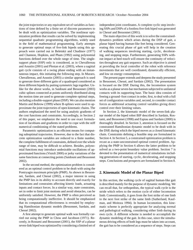
Fig. 2. Rear foot at toe-off, and front foot at heel-touch.
t ∈ [t t , t f ] ,{C1(q(t)) ≡ Oi
1At
6 · X0 − L+ � = 0 , (3)C2(q(t)) ≡ Oi
1At
6 ·Y0 = 0, (4)
∈ [t t + ε, tf ] , C3(q(t)) ≡ φ(q(t)) = 0. (5)
In eq. (2),β is the angle of the foot triangle at the tip Bi6(Figure 2).
ConstraintsC1 andC2 in eqs. (3) and (4) specify the Carte-sian coordinates of the contact pointAt
6 of the heel of the frontfoot. In eq. (3),L and� denote the step and foot lengths, re-spectively. In eq. (5),φ represents the inclination angle of thefront foot with the ground;ε is a short duration, after whichthe front foot remains flat on the ground, as specified by theconstraintC3.
In the following, constraints such as eqs. (3), (4), and(5) will be put together in the vector-valued functionCh de-fined as
Ch(q) = (C1(q), ..., Cnh(q))T , (6)
wherenh is the number of closure (or holonomic) constraints(nh = 2 or 3, above).
Moreover, the Jacobian matrix
���(q) = ∂Ch/∂q (7)
is used in the next section for deriving the Lagrange equationof motion.
Another approach could be used to describe the closedkinematics of the biped. Some authors, such as Azevedo,Poignet, and Espiau (2002), Chevallereau and Aoustin (2001)and Saidouni and Bessonnet (2003), cut all ground contactsand consider the biped as a free system in the two-dimensionalCartesian space. The Cartesian coordinates of the hip point areadded to the seven joint coordinates to describe the biped mo-tions. Two or three further closure conditions formulated atthe rear foot level are added to the above constraints (2)–(5).The main interest of this description lies in the fact that it al-lows the formulation of motion equations to be identical for
the two step phases. Nevertheless, the approach described be-low leads to a less constrained problem that is also simpler toformulate.
Absolute joint coordinates defined in Figure 1 lead tothe formulation of a concise dynamic model. No three-dimensional model of the biped would benefit from this sim-pler description. In this case, introducing a set of relativejoint coordinates, defined for instance using the well-knownDenavit–Hartenberg construction, becomes necessary.
3. Constrained Dynamic Model
As we want to formulate motion equations using a full set ofdependent configuration variables, this approach will resultin proposing a constrained dynamic model. Moreover, as weintend to implement the PMP, a state equation formulated instate space form is required. Special attention is devoted toboth the above dynamic modeling aspects in the followingsubsections.
3.1. Basic Dynamic Formulation
As stated in Section 2, in both motion phases the biped is as-sumed to be an open kinematic chain, the front foot contactbeing explicitly specified through closure constraints. Thiskinematic description results in stating a Lagrangian dynamicmodel with Lagrange multipliers, subjected to geometric clo-sure conditions, i.e., holonomic constraints. Lagrange equa-tions may be formulated as the generalnq-vector equation
M (q)q + C(q, q)+ G(q) = D (q, q)+ Bτττ +���T (q)λλλ,(8)
whereM is the biped mass-matrix,C contains centrifugaland Coriolis inertia terms,G and D represent gravity anddissipative terms, respectively,τττ is thenq-vector of actuatingjoint torques, defined asτττ = (0, τ2, ..., τnq )
T (τ1 = 0 meansthat, unlike the human foot, the tip of the foot is not actuated),λλλ is the Lagrangenh-vector multiplier associated to holonomicconstraintsCh, andB is a matrix that depends on the choiceof joint coordinates.
Equation (8) is the basic dynamic model we need to beginwith. In fact, this equation cannot be dissociated from con-straints (6) (or, equivalently, constraints (3)–(5)). This doublesystem of relationships is a set of differential-algebraic equa-tions. As discussed in Chessé and Bessonnet (2001) it needsto be especially adapted for implementing the PMP. With thisaim in view, a first requirement is to restate the Lagrangeequations in Hamiltonian form.
3.2. Hamiltonian Dynamic Model
Hamiltonian formalism is not in widespread use in the fieldof multibody system dynamics. Nevertheless, as shown in
Bessonnet, Chessé and Sardain / Optimal Gait Synthesis 1063
Bessonnet, Sardain, and Chessé (2002), a dynamic state equa-tion formulated in Hamiltonian canonic variables has a math-ematical structure that is perfectly appropriate for implement-ing the PMP, that is to say for deriving the necessary optimalityconditions stated by the maximum principle itself.
The reader is referred to Bessonnet, Sardain, and Chessé(2002) for specific statements related to Hamiltonian dynamicequations. In brief, we can recall that they are derived fromthe Lagrange equations by means of a change of variables thatconsists of substituting the conjugate momentump = ∂T /∂q(the Legendre transformation, whereT is the kinetic energyof the mechanical system) for the Lagrangian velocityq. Thenit can be shown (Bessonnet, Sardain, and Chessé 2002) thatthe Lagrangian vector-equation (8) splits up into twonq-ordersubsystems solved in the Hamiltonian phase velocities(q, p)as follows{
q = M−1(q)p ≡ g(q,p),
p = 1/2gTM ,qg − G(q)+ D(q,g(q,p))+BτBτBτ +���T (q)λλλ,(9)
whereM ,q ≡ ∂M/∂q.At this point, two types of variables must be identified, as
follows.
• The state variables of the controlled mechanical system,which are simply the Hamiltonian phase variables (orcanonic variables)q andp that we put together in the2nq-vectorx such asxT = (qT ,pT ).
• The control variables, which are the joint actuatingtorques. However, the multiplierλλλ represents efforts tobe applied to the front foot in order to hold this foot in itsspecified ground-contact position. Thus, it is possibleto add the components ofλλλ as complementary controlvariables. In this way, we are able to exert direct con-trol over the contact forces. These must obey specificconditions, as stated in Section 4.3. Consequently, wedefine the control vector on each phases by setting
t ∈ [t i , t t ] , u(t) = τττ(t) (10)
t ∈ [t t , t f ] , u (t)T = ( τττ (t)T , λλλ(t)T ). (11)
Equations (9) may be then restated on the first interval oftime as the 2nq-order differential equation
t ∈ [t i , t t ], x(t) = f (x(t))+ B u(t) ≡ F(x(t), u(t)), (12)
while, on the second, we have to deal with the differential-algebraic system
t ∈ [t t , t f ],
x(t) = f (x(t))+ B∗(x(t))u (t)
≡ F (x(t),u (t)), (13)
Ch(x(t)) = 0, (14)
whereB∗(x) ≡ (B,���T (x)).Both state equations (12) and (13) have the required form to
implement the PMP. We emphasize the fact that the Jacobianmatrix ∂F/∂x of F in eq. (13) must be derived exactly, inorder to benefit from accurate computation of the associatedadjoint system (45). This results from the implementation ofthe PMP, as shown below.
4. Defining a Feasible Step
Any feasible step obeys some specified conditions and limitsthe way we define a realistic gait which the biped will be ableto execute efficiently and control safely. Such specificationsdefined on the step cycle may be instantaneous or continuous.Also, they can apply to phase variables, as well as to controlinputs.
The first basic data to be introduced are the walk speeds,V . The step length,L, may be specified or optimized versusV . In any case, the step cycle timeT = t f − t i is defined bythe relationshipT = L/V . Moreover, settingTSS = t t − t i
andTDS = t f − t t , we consider that the DSP time representsabout 0.15%–0.25% of the cycle time as observed in humanwalking, i.e.,
TDS = T − TSS = k T ,0.15 � k � 0.25.
4.1. Transition Constraints
These are instantaneous constraints that characterize or definetransition postural configurations between the step phases. InFigure 1, the SSP–DSP cycle is depicted by three limitingconfigurations identified using superscriptsi, t , andf , as al-ready mentioned in Section 2. The step pattern is essentiallydefined by feet and hip positions and velocities at transitiontimest i , t t , andt f .
At initial time t i , the position and velocity of the tip Bi6 ofthe rear foot at toe-off must satisfy
OBi
6 = −Li X0,V(Bi
6) = 0 (15)
whereLi is the initial step length, whileV is the velocityvector.
It can be noted that many authors take into account heel-strike and introduce an equation of impact at transition be-tween successive steps (see, for example, Channon, Hopkins,and Pham 1992; Chevallereau andAoustin 2001; Plestan et al.2003). This means that velocities are discontinuous and sub-jected to instantaneous jumps from one step to the other. Sucha condition implies that accelerations have infinite jumps. Attransition timet t , this situation is avoided here, since we spec-ify, as advocated in Blajer and Schiehlen (1992), impactlessheel-touch at point At6 in order to prevent destabilizing effects

1064 THE INTERNATIONAL JOURNAL OF ROBOTICS RESEARCH / October–November 2004
on the motion control of the biped. Conditions to be satisfiedare similar to constraints (15), namely
OAt
6 = (Lf − �)X0, V(A t
6) = 0, (16)
whereLf is the final step length, and� is the foot length.At final time t f , the front foot being considered as flat on
the ground, we must have
OOf
6 = OOi
6 + LfX0, V(Of
6 ) = 0. (17)
Projecting the above six vector-relationships on ortho-normalized base vectorsX0 andY0 yields scalar relationships,which we write formally as
k � ntc ,
Cik(xL(t i)) = 0, (18)
Ctk(xL(t t )) = 0, (19)
Cf
k (xL(tf )) = 0, (20)
wherexL is the vector of the Lagrange phase variables,xTL
=(qT , qT ), andntc is here equal to 4.
If the step is cyclic, firstLf = Li = L and, secondly,xL(tf ) must be identified toxL(t i), given that the legs areswitched. Using the joint coordinate representation in Fig-ure 1, correlations betweenxL(tf ) andxL(t i) result from ex-changing initial and final coordinates as follows
qf
1 = qi6 + γ + π , qf
2 = qi5 + π , qf
3 = qi4 + π
qf
4 = qi3 − π , qf
5 = qi2 − π , qf
6 = −β − γ , qf
7 = qi7(21)
and swapping the joint velocities according to the scheme
k � 5 , qf
k = q i7−k , qf
6 = 0 , qf7 = q i7. (22)
Let us note that the relationships in eq. (22) appear sim-ply as the derivatives of relationships (21). Moreover, in thatcase, due to eqs. (21) and (22), constraints (20) are ipso factosatisfied.
Further conditions must be added to constraints (18)–(20)in order to ensure step feasibility. We have a choice betweentwo approaches. The first approach would be to limit the val-ues of key factors such as position and velocity of hip joint,inclination, and rotation rate of the trunk, and feet at toe-offand heel-touch. Such an approach would allow the transitionstatesxL(t i), xL(t t ), andxL(tf ) to be optimized while account-ing for constraints (18)–(20). A simpler approach would be tospecify the above factors as follows (see Figures 1 and 2 fornotations and symbols)
k = i, t, f
OOk
4 ·X0 = Xk4 , OOk
4 · Y0 = Y k4
V(Ok
4) ·X0 = V k4X , V(Ok
4) · Y0 = V k4Y
qk7∼= π/2 , qk7 ∼= 0
(23)
qi6 = δi6 − γ − π , qi6 = ω i6
qt6 = φt6 + α − π , qt6∼= 0
qf
1 = δf
1 , qf
1 = ωf
1
(24)
where quantities in the right-hand terms denote given values.The symbol “∼=” means that these values might be slightlydifferent from indicated ones. Then, relationships (18)–(20)can be solved inxL(t i), xL(t t ), andxL(tf ). In this way, tran-sition states are known and considered as simple boundaryvalue conditions. In Section 7, numerical simulations are per-formed using this approach.
4.2. State Constraints
As for any human movement or robot motion, joint trajec-tories of walking machines must be subjected to a limitedrange in order to avoid unfeasible movements, such as jointcounter-flexion, or ground and obstacle collisions. Such nec-essary constraints cannot be omitted. They involve joint coor-dinates and velocities considered throughout the cycle time.Considering relative joint coordinates defined as (Figure 1)
ϕ1 = θ1, ϕi = θi − θi−1 , i = 2, ..., nq,
joint motion limitations and counter-flexing avoidance at kneeand ankle level must be taken into account by setting
t ∈ [t i , tf ] ,
ϕ min
5 � ϕ 5(t) � 0
−γ � ϕ 6(t) � 0
0 � ϕ 3(t) � ϕ max3
. (25)
The first two double inequalities relate to the knee andankle of the swing leg. The third refers to the knee of thestance leg, which becomes the rear leg during the DSP. Wecan rewrite the six above inequalities in the generic form
t ∈ [t i , tf ] , CS
j(x(t)) � 0 , j = 1, ...,6. (26)
Let us note that joint velocities could be moderated usingsimilar inequalities.
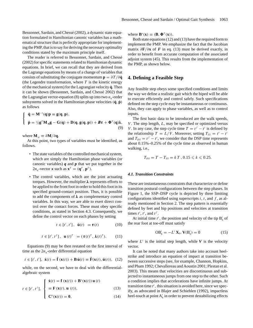
Further constraints must be stated to enable swing footclearance from the ground, and stepping over an obstacle, ifneeded. In Figure 3, bell-shaped curves are used to define ex-clusion zones from which the foot must be removed upwards.
The lower curve may be used for specifying foot clearance,and the upper one for obstacle avoidance. This approach wasfirst introduced in Rostami and Bessonnet (2001). Here, weuse a simpler algebraic description of the curve by consideringthe fourth-order polynomial function
x ∈ [a, b] , f (x) = h
((x − a)(b − x)
(c − a)(b − c)
)2
wherea andb represent the abscissa of points situated be-tween, or coinciding with, the toe-off point Bi6 and the heel-touch point At6. The functionf satisfies obviouslyf (a) =
Bessonnet, Chessé and Sardain / Optimal Gait Synthesis 1065
)( Axf
)(xfAy
0 i6B t
6AxAx c
a b
B
A
)( Axf
)(xfAy
0 i6B t
6AxAx c
a b
B
A
Fig. 3. Foot clearance and obstacle avoidance.
f (b) = 0, f (c) = h, f ′(a) = f ′(b) = 0, andf ′(c) = 0,provided thatc = (a + b)/2. Therefore,h defines the maxi-mum clearance height. This need only be a few centimeters forwalking on level ground. Foot clearance is considered to beeffective if the foot sole remains clear of the curve. Fulfillmentof this condition by sole ends A and B may be sufficient toprevent any ground collision. Using the notations in Figure 3,such a condition is expressed by the set of inequalities
f (xA)− yA � 0, f (xB)− yB � 0
wherexA, xB , yA, andyB must be formulated as functions ofthe state variables, reduced here to the joint coordinates. It isthen possible to restate the above constraints in a form similarto eq. (21), i.e.,
t ∈ [t i , t t ] , CS
j(x(t)) � 0 , j = 7,8. (27)
A third constraint formulated for the middle point of thesole might be added to improve the fulfillment of clearancecondition.
4.3. Sthenic Constraints
We use the term sthenic constraints (sthenic is from Greeksthenos meaning “force”), for restrictions formulated on ac-tive and passive interacting forces that are at work and at stakein the kinematic chain. First, technological limitations of ac-tuators need to keep actuating torques within limits such that
t ∈ [t i , tf ] , τmini
� τi(t) (≡ ui(t)) � τmaxi, i = 2, ...,7.
(28)
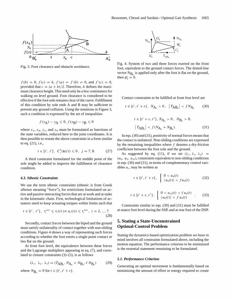
Secondly, contact forces between the biped and the groundmust satisfy unilaterality of contact together with non-slidingconditions. Figure 4 shows a way of representing such forcesaccording to whether the foot exerts a single point contact orlies flat on the ground.
At front foot level, the equivalence between these forcesand the Lagrange multipliers appearing in eq. (7), and corre-lated to closure constraints (3)–(5), is as follows
(λ1, λ2, λ3) = (TAB6, NA6
+NB6, �NB6
) (29)
whereNB6= 0 for t ∈ [t t , t t + ε] .
6ABT
6BN6AN
t6O
t6A
t6B
t6f
Fig. 4. System of two and three forces exerted on the frontfoot, equivalent to the ground contact forces. The dotted-linevector NB6
is applied only after the foot is flat on the ground,thenφt6 = 0.
Contact constraints to be fulfilled at front foot level are
t ∈ [t t , t t + ε] , NA6> 0 ,
∣∣ TAB6
∣∣ < fNA6(30)
t ∈ [t t + ε, tf ] , NA6> 0 , NB6
> 0,∣∣ TAB6
∣∣ < f (NA6+NB6
). (31)
In eqs. (30) and (31), positivity of normal forces means thatthe contact is unilateral. Non-sliding conditions are expressedby the remaining inequalities wheref denotes a dry-frictioncoefficient between the foot sole and the ground.
As suggested by eq. (11), if we set(λ1, λ2, λ3) =(u8, u9, u10), constraints equivalent to non-sliding conditionsin eqs. (30) and (31), in terms of complementary control vari-ablesui , may be written as
t ∈ [t t , t t + ε] ,{
0< u9(t)
| u8(t)| < fu9(t)(32)
t ∈ [t t + ε, tf ] ,{
0< u10(t) < � u9(t)
| u8(t)| < f u9(t). (33)
Constraints similar to eqs. (30) and (31) must be fulfilledat stance foot level during the SSP, and at rear foot of the DSP.
5. Stating a State-UnconstrainedOptimal-Control Problem
Stating the dynamics-based optimization problem we have inmind involves all constraints formulated above, including themotion equation. The performance criterion to be minimizedis the essential statement remaining to be formulated.
5.1. Performance Criterion
Generating an optimal movement is fundamentally based onminimizing the amount of effort or energy required to create
1066 THE INTERNATIONAL JOURNAL OF ROBOTICS RESEARCH / October–November 2004
the motion.The energy criterion presents some disadvantages.First, resulting optimal actuating torques have discontinuousvariations of bang-zero-bang type (see, for example, Lewisand Syrmos 1995). The consequences would be movementsexecuted with repeated backlashes on the joint axis.This couldhave destabilizing effects on the biped control. Secondly, dueto the abovementioned discontinuities, the problem is non-smooth and cannot be solved satisfactorily. A performancecriterion, defined as the integral quadratic amount of drivingtorquesτi and reaction forcesλj , represents a suitable choicefor dealing with optimal dynamics of jointed multibody sys-tems which have closed kinematics. Thus, we consider thedouble criterion (with notations from eqs. (10) and (11))
JSS(u) = 1
2
t t∫t i
u(t)TDuu (t) dt ≡ 1
2
t t∫t i
τττ (t)TDττττ (t) dt
(34)
JDS(u) = 1
2
tf∫t t
u (t)Du u (t)dt
≡ 1
2
tf∫t t
(τττ (t)TDττττ (t)+ λλλ(t)TDλλλλ(t)) dt. (35)
In eqs. (34) and (35),Dτ andDλ,or equivalentlyDu andDu,are diagonal weighting matrices. Initially, only unity matricesare considered. Then, if we want the optimization process togive more (less) input to torquesτ i , or interacting forcesλj ,the corresponding weighting coefficients will be set at val-ues smaller (greater) than unity. The effect expected can onlybe revealed by carrying out numerical tests. Values between0.5 and 2 could be sufficient for producing results showingsignificant differences.
Minimizing the quadratic values of actuating torques en-sures their continuity. Moreover, the biped being essentiallysubjected to gravity forces, such a criterion will favor uprightwalking patterns which require little effort to support the bipedweight. The quadratic term inλ is aimed at minimizing antag-onistic forces, especially sliding forces, which might appearin the locomotion system during the DSP.
Bounds introduced in eq. (28) on control variablesτi(i �nτ = 7) define, during the SSP, a set of feasible values, whichis a parallelepiped in annτ -dimensional Euclidian space. Wewill denote this feasible set asU . During the DSP, bounds(28) together with constraints (32) and (33) prescribed forcomplementary control variablesu7+j ≡ λj(j � nλ, nλ =2 or 3) define, in an(nτ + nλ)-dimensional Euclidian space,a set with polyhedral geometry which has right and obliquefaces. It is a time-dependent convex polytope in which theabove criterion (35) must be minimized. We will label thisfeasible setU(t), in which optimal controlu has to be foundduring the DSP.
5.2. State-Unconstrained Optimal-Control Problem
Dealing directly with state inequality constraints such aseqs. (26) and (27), using the PMP, leads to quite involvednon-smooth optimal conditions (Pontryagin et al. 1962; Ioffeand Tihomirov 1979) that make the optimal control prob-lem practically unsolvable. An alternative approach is to im-plement a penalty technique. This resembles methods usedto solve mathematical programming problems. An exteriorpenalty method, as used in Chessé and Bessonnet (2001) andBessonnet, Chessé, and Sardain (2002), is easy to implement,and proved to be computationally efficient. It consists of min-imizing the integral amount of the constraints wherever theyare an infringement. To that end, let us group together in-equality state constraints (26) and (27) in the vector-valuedfunctionCS(x (t)) such that
CS = (CS
1 , ..., CS
nS)T , (nS � 8).
Then, setting
t ∈ [t i , tf ] , CS+i(x(t)) = Max(0, CS
i(x(t))) ;
CS+ = (CS+1 , ..., CS+
nS)T ,
we define the quadratic penalty functionψS such that
ψS(x) = 12[CS+(x)]TDSCS+(x). (36)
Moreover, we deal with state equality constraints (14) us-ing a similar approach, by introducing the second penaltyfunction
t ∈ [t t , t f ] , ψh(x(t)) = 12[Ch(x(t))]T Dh Ch(x(t)). (37)
In eqs. (36) and (37),DS andDh denote diagonal weightingmatrices. Both of the above functions will be minimized byconsidering the augmented criteria
J ∗SS(u) = JSS(u)+ rS
tf∫t i
ψS(x(t)) dt (38)
J ∗DS(u) = JDS(u)+
tf∫t t
[rSψS(x(t))+ rhψh(x(t))] dt (39)
whererS andrh are penalty factors. In theory, it can be shownthat penalty functions vanish through the minimization of thecost function when penalty factors tend towards infinity (Leleand Jacobson 1969). In fact, reasonably high given valueswill enable the penalty functions to have negligible residualvalues. The reader is referred to the beginning of Section 7for numerical examples.
At this point, the state-unconstrained optimal-control prob-lem we intend to solve can be summarized as follows
for rS great,
{minimize
u∈UJ ∗SS(u), (40)
andrh great, minimizeu∈U(t)
J ∗DS(u), (41)

Bessonnet, Chessé and Sardain / Optimal Gait Synthesis 1067
while satisfying the state equations
t ∈ [t i , t t ] , x(t) = F(x(t), u(t)), (42)
t ∈ [t t , t f ] , x(t) = F(x(t),u(t)), (43)
together with either the boundary constraints
k = 1, ..., 4
Cik(xL(t i)) = 0
Ctk(xL(t t )) = 0
Cf
k (xL(tf )) = 0
(44)
or the boundary conditions
xL(t i) = xiL
xL(t t ) = xtL
xL(tf ) = xfL. (45)
In the latter case,xiL, xt
L, andxfL denote given values.
As we want to optimize both step phases separately, theabove problem will be split into two independent optimizationproblems set on the intervals of time[t i , t t ] and[t t , t f ] of theSSP and DSP of the gait, respectively.
6. Solving a Two-Point Boundary Value Problem
The presentation is focused on the DSP which adds to the char-acteristics of the SSP, quite restrictive geometric and sthenicclosure conditions. Nevertheless, both problems as stated ineqs. (40), (41) and (42), (43), each being completed with con-ditions (44) or (45), are formally identical. Indeed, differencesbetween the two problems, due to additional terms appearingin the second, expand when deriving necessary conditions ofoptimality stated by the PMP.
The reader is referred to textbooks and monographs suchas Pontryagin et al. (1962), Ioffe and Tihomirov (1979), andLewis and Syrmos (1995) for details concerning the formula-tion of the PMP. In fact, as the final optimal control problemwe have to deal with is unconstrained in the state, optimalityconditions are formally quite easy to derive.
We assume that constraints (44) are solved in the statexL through relationships (21)–(24). Therefore, we take onlyboundary conditions (44) into consideration. In this way, theoptimization problem to be solved consists of determining astate vector-functiont → x(t) and a control vector-functiont → u(t) ∈ U(t) minimizing the augmented criterion (41),while satisfying the state equation (43) together with theboundary conditions (45).
Setting
L(x,u) = uTDuu + rSψS(x)+ rhψh(x)
for the Lagrangian of criterionJ ∗DS
in eq. (39), and definingthe Hamiltonian function
w ∈ �nq , H(x, u, w) = wTF(x, u)− L(x, u),
the PMP states that, ift → (x(t),u(t)) is a solution ofeqs. (42), (43), and (45), then a 2nq-vector adjoint functiont → w(t) exists such thatt → (x(t),u(t),w(t)) satisfies theadjoint equation
t ∈ [t t , t f ] , w(t) = −(∂H/∂ x)T
≡ −(∂F/∂x)Tw + (∂L/∂x)T (46)
and the maximality condition of the Hamiltonian
t ∈ [t t , t f ] , H(x(t),u (t),w(t)) = Maxv∈U(t)
H(x(t), v,w(t)).
(47)
Condition (47) plays a key role in dealing with the controlvectoru. It allowsu to be expressed, at every timet , as a func-tion of both the state and the co-state vector variablesx andw, that isu(t) = U(x(t),w(t)). Substituting this expressionfor u in state and co-state equations (43) and (46) yields the4nq-order differential system
t ∈ [t t , t f ] ,{
x(t) = F∗(x(t),w(t))w(t) = G∗(x(t),w(t))
, (48)
in which the state variablex must satisfy the 4nq endconditions {
x(t t ) = xt
x(tf ) = xf(49)
derived from eq. (45).The two-point boundary value problem (48), (49) can be
solved using existing algorithms. The numerical techniqueswe use are described in Bessonnet, Sardain, and Chessé(2002). The method involves solving the problem in twostages. In the first stage, we are searching for a guess solutionby implementing an easy-to-use shooting method describedin Bryson and Ho (1975), and based on the construction of atransition matrix algorithm. As this technique lacks numeri-cal robustness, the problem is solved with null penalty factorsrS and rh, these giving rise to some stiff numerical condi-tioning. In the second stage, the problem is solved iterativelyfor increasing values ofrS andrh using the routine D02RAFof the NAG FORTRAN Library, which implements a finite-difference algorithm. This computing code is quite efficient,and withstands sufficiently high values of penalty factors forhaving non-significant final residual values of both penaltyfunctions.
7. Generating an Optimal Walking Sequence
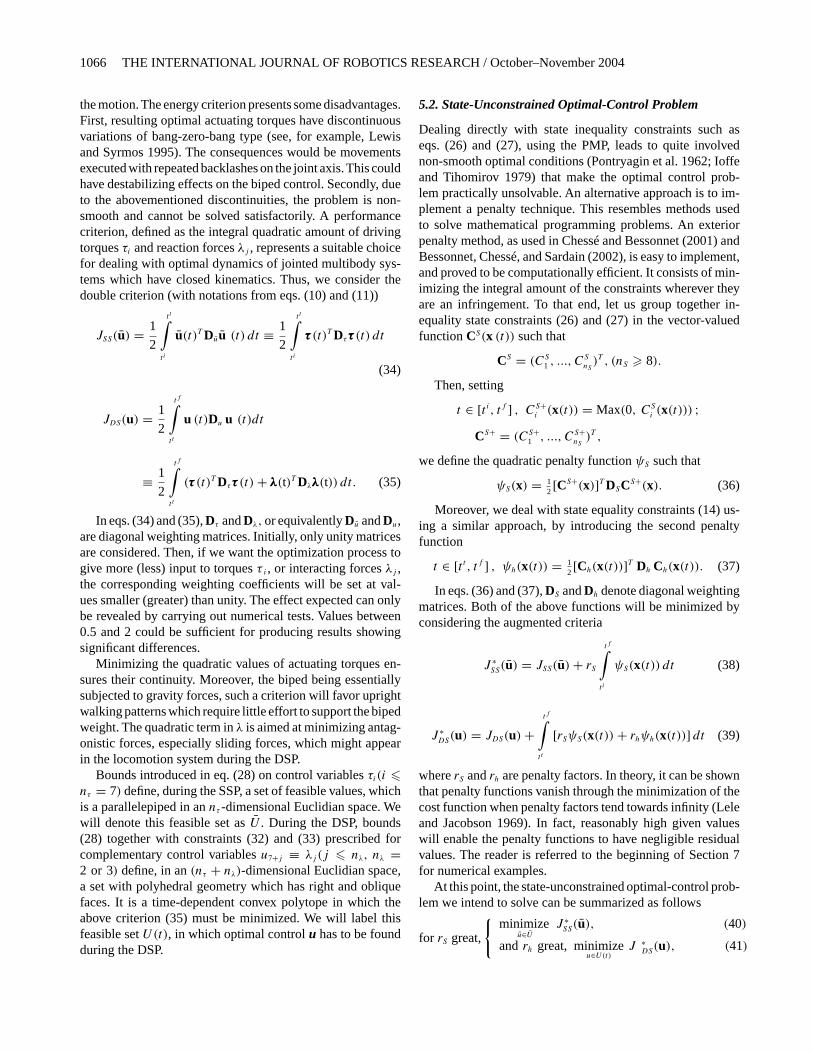
In this section we present results concerning the construc-tion of a walking sequence on level ground. This comprisesstarting, cyclic, decelerating, and stopping steps. Computa-tions were carried out on the basis of numerical data given inTable 1. These data represent the mechanical characteristics
1068 THE INTERNATIONAL JOURNAL OF ROBOTICS RESEARCH / October–November 2004
Table 1. Mechanical Design Parameters of the Biped BIP (Figure 5)
Link Li L1 L2 L3 L4 L5 L6 L7
Lengthri (m) 0.188 0.410 0.410 0.410 0.410 0.290 0.146Massmi (kg) 2.340 6.110 10.900 10.900 6.110 2.340 66.110ai (m) 0.143 0.258 0.250 0.160 0.152 0.045 0.391bi (m) 0.042 0.028 0.005 –0.005 –0.028 –0.042 0.029Ii (m2kg) 0.100 0.690 1.310 1.020 0.720 0.070 18.990
Centers of gravity are defined by setting OiGi = aixi + biyi (Figure 1),xi = OiOi+1/ri , yi = z0 × xi . Ii refers to the momentof inertia of link Li about Oi .
Fig. 5. The biped BIP and its locomotion system: 15 degreesof freedom, 1.8 m, 107 kg (LMS, University of Poitiers, andINRIA- R.A., France).
of the biped BIP (Figure 5) when considered to be movingin its sagittal plane. A cyclic step is first presented becauseits transition kinematic characteristics are required to definestarting and stopping steps.
Penalty factorsrS andrh introduced in eqs. (38) and (39)were set at 150. It should be noted that the residual distancefrom the position of pointAt6 computed on the basis of closureconstraints (3) and (4) to its assigned position never exceeds0.3 mm.
7.1. Cyclic Step
A purely cyclic step is defined (as described in Section 4.1) byconditions (18) and (19), together with the swapping relation-ships (21) and (22) at the end of the cycle. Such conditionsneed some complementary data. Walk speed is the most sig-nificant one. In the simulation presented here, it is equal to0.75 m s−1 (2.7 km h−1), which represents a fairly fast walk.After a few numerical tests, the corresponding step length wasset at 0.5 m, while the motion time of the DSP was set at 0.25%of the total cycle time.
A stick diagram of the optimal motion is shown in Figure 6.The gait pattern has particular characteristics. First, the legs
(DSP) (SSP)
Fig. 6. Cyclic optimal step (sagittal DSP and SSP) of thebiped BIP.
are slightly flexed in order for the foot of the stance leg toremain flat on the ground during the whole swing phase. Sec-ondly, at the end of the swing phase, heel-touch takes placewithout impact. These two specific features are expected toensure safer control of gait.
In Figure 7, actuating torques show few variations and re-main at fairly moderate values (Tij is the torque exerted bylink Li (i = 2, . . . ,7) on linkLj(j = 1, . . . ,6)). Althoughthe ground contact conditions represent very restrictive con-straints, time charts of ground interaction forces in Figure 8show they are perfectly fulfilled. During both phases, all nor-mal components of the contact forces are positive. Moreover,normal components NB1 and NA6B6 (NA6B6 is a short no-tation for NA6+NB6) during the double support, and normalcomponents NA6 and NB6 during the single support, crosseach other during their respective phases. This indicates thatthere is a steady transfer of the biped weight forward. Note alsothat the horizontal components, TAB1 and TAB6, never ex-ceed 20% of normal ones. Therefore, little grip on the groundis needed to avoid sliding. It can be seen also that, at the begin-ning of the double support, the biped lifts its weight off theground. Conversely, at the beginning of the single support,there is an increase in the normal supporting force as the hiprises.
In Figure 9, note that the seventh joint velocity V(L6/gd),referring to the rotation rate of link L6 versus the ground, is
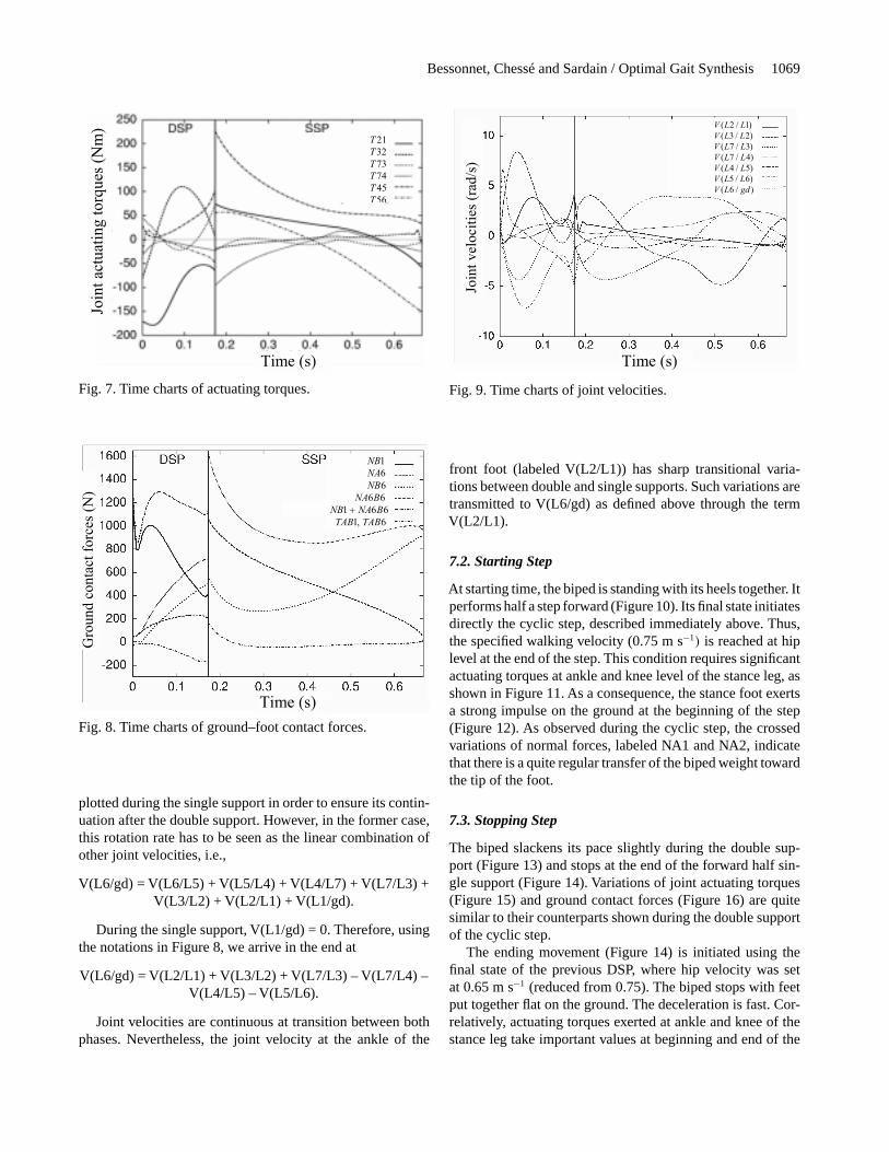
Bessonnet, Chessé and Sardain / Optimal Gait Synthesis 1069
Time (s)
Join
t ac
tuat
ing t
orq
ues
(N
m)
56
45
74
73
32
21
T
T
T
T
T
T
Fig. 7. Time charts of actuating torques.
Time (s)
Gro
und c
onta
ct f
orc
es (
N)
6,1
661
66
6
6
1
TABTAB
BNANB
BNA
NB
NA
NB
Fig. 8. Time charts of ground–foot contact forces.
plotted during the single support in order to ensure its contin-uation after the double support. However, in the former case,this rotation rate has to be seen as the linear combination ofother joint velocities, i.e.,
V(L6/gd) = V(L6/L5) + V(L5/L4) + V(L4/L7) + V(L7/L3) +V(L3/L2) + V(L2/L1) + V(L1/gd).
During the single support, V(L1/gd) = 0. Therefore, usingthe notations in Figure 8, we arrive in the end at
V(L6/gd) = V(L2/L1) + V(L3/L2) + V(L7/L3) – V(L7/L4) –V(L4/L5) – V(L5/L6).
Joint velocities are continuous at transition between bothphases. Nevertheless, the joint velocity at the ankle of the
)/6(
)6/5(
)5/4(
)4/7(
)3/7(
)2/3(
)1/2(
gdLV
LLV
LLV
LLV
LLV
LLV
LLV
Time (s)
Join
t v
elo
citi
es (
rad
/s)
Fig. 9. Time charts of joint velocities.
front foot (labeled V(L2/L1)) has sharp transitional varia-tions between double and single supports. Such variations aretransmitted to V(L6/gd) as defined above through the termV(L2/L1).
7.2. Starting Step
At starting time, the biped is standing with its heels together. Itperforms half a step forward (Figure 10). Its final state initiatesdirectly the cyclic step, described immediately above. Thus,the specified walking velocity (0.75 m s−1) is reached at hiplevel at the end of the step. This condition requires significantactuating torques at ankle and knee level of the stance leg, asshown in Figure 11. As a consequence, the stance foot exertsa strong impulse on the ground at the beginning of the step(Figure 12). As observed during the cyclic step, the crossedvariations of normal forces, labeled NA1 and NA2, indicatethat there is a quite regular transfer of the biped weight towardthe tip of the foot.
7.3. Stopping Step
The biped slackens its pace slightly during the double sup-port (Figure 13) and stops at the end of the forward half sin-gle support (Figure 14). Variations of joint actuating torques(Figure 15) and ground contact forces (Figure 16) are quitesimilar to their counterparts shown during the double supportof the cyclic step.
The ending movement (Figure 14) is initiated using thefinal state of the previous DSP, where hip velocity was setat 0.65 m s−1 (reduced from 0.75). The biped stops with feetput together flat on the ground. The deceleration is fast. Cor-relatively, actuating torques exerted at ankle and knee of thestance leg take important values at beginning and end of the
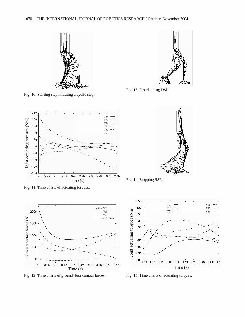
1070 THE INTERNATIONAL JOURNAL OF ROBOTICS RESEARCH / October–November 2004
Fig. 10. Starting step initiating a cyclic step.
Join
t ac
tuat
ing t
orq
ues
(N
m)
21
32
73
74
45
56
T
T
T
T
T
T
Time (s)
Fig. 11. Time charts of actuating torques.
Time (s)
Gro
un
d c
on
tact
fo
rces
(N
)
1
1
1
11
TAB
NB
NA
NBNA
Fig. 12. Time charts of ground–foot contact forces.
Fig. 13. Decelerating DSP.
Fig. 14. Stopping SSP.
Join
t ac
tuat
ing t
orq
ues
(N
m)
Time (s)
73
32
21
T
T
T
56
45
74
T
T
T
Fig. 15. Time charts of actuating torques.

Bessonnet, Chessé and Sardain / Optimal Gait Synthesis 1071
Join
t ac
tuat
ing t
orq
ues
(N
m)
Time (s)
73
32
21
T
T
T
56
45
74
T
T
T
Fig. 16. Time charts of ground–foot contact forces.
Join
t ac
tuat
ing t
orq
ues
(N
m)
Time (s)
21
32
73
74
45
56
T
T
T
T
T
T
Fig. 17. Time charts of actuating torques.
movement (Figure 17). Similarly, the normal ground reactionforce (Figure 18) shows high values at the same moments asabove. We can see that the system of two forces NA1 and NA2applied at the ends of the sole, and equivalent to uniformlydistributed normal interaction forces, ends with values closeto each other. This result shows that the biped is statically wellbalanced after stopping.
The four motions described above are assembled in thewalking sequence shown in Figure 19. We can observe thatthe trunk leans forward slightly, especially during the cyclicand stopping steps.
Gro
un
d c
on
tact
fo
rces
(N
)
Time (s)
122121
TANANAANA
Fig. 18. Time charts of ground–foot contact forces.
Fig. 19. Optimal walking sequence comprising starting,cyclic, and stopping steps.
7.4. Energetic Cost
The energy expended during each elementary movement wascomputed using
E =t2∫
t1
7∑i=2
|ϕi(t)τi(t)| dt
wheret1 andt2 are some initial and final times.The energetic cost of the cyclic step amounts to 205.8 J
(96.3 J for the only DSP). The starting step requires 81.9 J.
1072 THE INTERNATIONAL JOURNAL OF ROBOTICS RESEARCH / October–November 2004
The stopping step needs 112.1 and 105.1 J during the dou-ble support and single support, respectively. Thus, the totalamount of energy expended to create the walking sequenceshown in Figure 18 is equal to 504.9 J. In addition, the powerrequired to perform a steady walk generated on the basis ofthe cyclic step, amounts to 307 W. The above energetic ex-penditure is greater than its human counterpart during normalgait. In fact, the gait generated is not really human-like. Inparticular, the biped keeps its knees flexed in order to main-tain its stance foot flat on the ground during swing phases. Inhuman gait, the heel of the stance foot lifts up before the endof such phases, making the transition towards the next dou-ble support smoother. Moreover, as heel-touch takes placewithout impact, the biped must tightly control its swing legat the end of the single support. On the other hand, a goodmeans of lowering the energetic expenditure, and making themovement smooth, would be to optimize the transition stateslinking two successive phases. This is future work.
8. Concluding Remarks
Legged-locomotion systems perform as time-varying me-chanical structures and obey quite restrictive constraints. Inthis respect, two specific aspects of gait require particularattention. First, there is the unilaterality of ground–foot con-tacts, which affects the biped equilibrium and strictly limitsthe set of feasible solutions. Secondly, during the DSP ofbipedal gait, the biped moves as a closed-loop kinematic sys-tem. In that case, for any joint trajectories, there is a continuumof solutions in terms of joint actuating torques. This indeter-minacy could yield inappropriate distribution of actuating in-puts in the locomotion system. It could then be the cause ofantagonistic forces exerted between legs. The most likely con-sequence of this would be contact loss and sliding. The paperis especially focused on this particular phase of gait. The ap-proach developed involves opening the closed loop at groundcontact level in order to formulate a simple dynamic modeland to obtain direct control over the contact forces. Indeed,the latter, especially horizontal grip forces, are considered ascomplementary control variables. This helps the process offinding optimal inputs directly compatible with non-slidingconditions. Closure conditions are taken into account simplythrough the minimization of a penalty function. In this way,the problem stated for generating optimal DSPs is formallyquite similar to their SSP counterparts.
The approach presented may be completed consideringvarious aspects of the optimization problem. First, posturalconfigurations of the biped at transition between successivephases could be optimized in order to obtain smoother and lessenergy-consuming gait cycles. Secondly, dividing the SSPinto two subphases in order to allow the stance foot to rotateabout its tiptoe axis before heel-touch of the swing foot wouldcontribute to smooth the transition from single support to dou-
ble support. Thirdly, gait cycles could be globally optimized.In this case, necessary optimality conditions stated using thePMP would lead to anN -point boundary value problem withN � 3.
Generating three-dimensional gait is not basically differ-ent from generating sagittal gait. However, due to the greaterkinematic complexity, stating the optimization problem wouldrequire a great deal of effort. Furthermore, solving algorithmscould be quite sensitive to this greater complexity. Neverthe-less, lateral movements of three-dimensional bipeds have lim-ited range with smooth variations during normal gait. For thisreason, the numerical conditioning of stated problems mightbe only moderately modified.
Finally, a good challenge would be to generate optimalsteps using updated constraints at every time in order to ac-count for external disturbances. In other words, the optimiza-tion problem would be stated and solved at current timet
with updated constraints to generate the finishing step. Solv-ing such a problem in real time, as is required, seems beyondthe reach of current algorithms and computers. However, ifconstraint disturbances are not too stiff, the solution att+ δtwill be very close to the solution at timet . The latter could beefficiently used to initiate and obtain a rapid numerical con-vergence toward the new solution att+ δt, and so on. Such anapproach would be useful to generate and control unsteadygait of biped robots walking in a fluctuating environment.
References
Azevedo, C., Poignet, P., and Espiau, B. 2002. Moving horizoncontrol for biped robots without reference trajectory.Pro-ceedings of the IEEE International Conference on Roboticsand Automation (ICRA), Seoul, Korea, pp. 2762–2767.
Beletskii, V.-V., and Chudinov, P.-S. 1977. Parametric opti-mization in the problem of biped locomotion.Mechanicsof Solids 12(1):25–35.
Bessonnet, G., Chessé, S., and Sardain, P. 2002. Generatingoptimal gait of a human-sized biped robot.Proceedings ofthe 5th International Conference on Climbing and WalkingRobots, Paris, France, pp. 717–724.
Bessonnet, G., Sardain, P., and Chessé, S. 2002. Optimal mo-tion synthesis – dynamic modeling and numerical solvingaspects.Multibody System Dynamics 8:257–278.
Blajer, W., and Schiehlen, W. 1992. Walking without impactsas a motion/force control problem.ASME Journal of Dy-namic Systems, Measurement, and Control 114:660–665.
Bryson, A.E., and Ho, Y.C. 1975.Applied Optimal Control,Hemisphere, New York.
Channon, P.-H., Hopkins, S.-H., and Pham, D.-T. 1992.Derivation of optimal walking motions for a bipedal walk-ing robot.Robotica 10:165–172.
Chessé, S., and Bessonnet, G. 2001. Optimal dynamics ofconstrained multibody systems. Application to bipedalwalking synthesis.Proceedings of the IEEE International
Bessonnet, Chessé and Sardain / Optimal Gait Synthesis 1073
Conference on Robotics and Automation (ICRA), Seoul,Korea, pp. 2499–2505.
Chevallereau, C., andAoustin,Y. 2001. Optimal reference tra-jectories for walking and running of a biped robot.Robot-ica 19:557–569.
Chow, C.-K., and Jacobson, D.-H. 1971. Studies of humanlocomotion via optimal programming.Mathematical Bio-sciences 10:239–306.
Espiau, B., and Sardain, P. 2000. The anthropomorphic bipedrobot BIP 2000.Proceedings of the IEEE InternationalConference on Robotics and Automation (ICRA), San Fran-cisco, CA, pp. 3997–4002.
Fujimoto,Y., Obata, S., and Kawamura,A. 1998. Robust bipedwalking with active interaction control between foot andground.Proceedings of the IEEE International Conferenceon Robotics and Automation, Leuven, Belgium, pp. 2030–2035.
Hirai, K., Hirose, M., and Takenaka, T. 1998. The devel-opment of Honda humanoid robot.Proceedings of theIEEE International Conference on Robotics and Automa-tion (ICRA), Leuven, Belgium, pp. 160–165.
Inoue, K.,Yoshida, H.,Arai, T., and Mae,Y. 2000. Mobile ma-nipulations of humanoids – real-time control based on ma-nipulability and stability.Proceedings of the IEEE Inter-national Conference on Robotics and Automation (ICRA),San Francisco, CA, pp. 2217–2222.
Ioffe, A.-D., and Tihomirov, V.-M. 1979.Theory of ExtremalProblems, North-Holland, Amsterdam.
Kiriazov, K. 2002. Learning robots to walk dynamically – bi-ological control concepts.Proceedings of the 5th Interna-tional Conference on Climbing and Walking Robots, Paris,France, pp. 3–10.
Lele, M.-M., and Jacobson, D.-H. 1969. A proof of the con-vergence of the Kelley–Bryson penalty function techniquefor state-constrained control problem.Journal of Mathe-matical Analysis and Application 26:163–169.
Lewis, F.-L., and Syrmos,V.-L. 1995.Optimal Control,Wiley,New York.
Löffler, K., Gienger, M., and Pfeiffer, F. 2002. Trajectorycontrol of a biped robot.Proceedings of the 5th Interna-
tional Conference on Climbing and Walking Robots, Paris,France, pp. 437–444.
Martin, B.-J., and Bobrow J.-E. 1999. Minimum-effort mo-tions for open-chain manipulators with task-dependentend-effector constraints.International Journal of RoboticsResearch 18(2):213–224.
Muraro, A., Chevallereau, C., and Aoustin, Y. 2003. Opti-mal trajectories for a quadruped robot with trot, amble andcurvet gaits for two energetic criteria.Multibody SystemDynamics 9:39 –62.
Plestan, F., Grizzle, J.-W., Westervelt, E.-R., and Abba, G.2003. Stable walking of a 7-DOF biped robot.IEEE Trans-actions on Robotics and Automation 19(4):653 –668.
Pontryagin, L., Boltiansky, V., Gamkrelitze, A., andMishchenko, E. 1962.The Mathematical Theory of Op-timal Processes, Wiley Interscience, New York.
Rostami, M., and Bessonnet, G. 2001. Sagittal gait of a bipedrobot during the single-support phase, Part 2: optimal mo-tion. Robotica 19:241–253.
Saidouni, T., and Bessonnet, G. 2002. Gait trajectory opti-mization using approximation functions.Proceedings ofthe 5th International Conference on Climbing and Walk-ing Robots, Paris, France, pp. 709–716.
Saidouni, T., and Bessonnet, G. 2003. Generating globallyoptimized sagittal gait cycles of a biped robot.Robotica21:199–210.
Sardain, P., Rostami, M., and Bessonnet, G. 1998. An an-thropomorphic biped robot: dynamic concepts and tech-nological design.IEEE Transactions on Systems, Man andCybernetics 28A(6):823–838.
Sutherland, D.-H., Kaufman, K.-R., and Moitoza, J.-R. 1994.Kinematics of normal human gait.HumanWalking, J. Roseand J.G. Gamble, editors, Williams and Wilkins, Balti-more, MD, pp. 23–44.
Visioli, A. 2000. Trajectory planning of robot manipulatorsby using algebraic and trigonometric splines.Robotica18:611–631.
Vukobratovic, J., Borovac, B., Surla, D., and Stokic, D. 1990.Biped Locomotion: Dynamics, Stability, Control and Ap-plications, Springer-Verlag, Berlin.