Optimal Hamiltonian Simulationby

Quantum Signal Processing Guang-Hao Low, Isaac L. Chuang

Massachusetts Institute of Technology

QIP 2017

January 19

1

Physics ↔ ComputationPhysical concepts inspire problem-solving techniques◦ Adiabatic evolution, Quantum walks

◦ Universal quantum computation

◦ Compiling to specific architecture has large overheads

Physical systems solve problems◦ Boson sampler, Analog quantum simulator

◦ Very elegant, simple, fast; Near future prospects

◦ Generally not fault-tolerant

Quantum Signal Processing: Abstraction of physical dynamics into a computing module `Quantum Signal Processor’ that◦ Preserve intuition of how original physical system computes

◦ Preserve simplicity, optimality of original physical system

◦ In a FTQC compatible manner

2

Outline

1. Hamiltonian Simulation

◦ A Brief History of Simulation

2. Overview of Algorithm

◦ Quantum Signal Processing

◦ Optimal Hamiltonian Simulation

3. Conclusion

3

1. Hamiltonian Simulation

4

Difficult for classical computers in generalCurse of dimensionality: 𝑛 qubits ⇒ 𝑁 = 2𝑛 states

PromiseBQP-complete

𝑖𝑑ȁ ۧ𝜓

𝑑𝑡= 𝐻ȁ ۧ𝜓 𝑒−𝑖 𝐻𝑡

“… nature isn’t classical, dammit, and if you want to make a simulation of nature, you’d better make it quantum mechanical, and by golly it’s a wonderful problem, because it doesn’t look so easy.”Richard Feynman (1982)

Run quantum algorithms:Quantum walks, span programs etc.

Simulate nature: Chemistry, materials, etc.

Assumptions𝒌-local interactions [Lloyd 1996]

• 𝐻 = σ𝑗=1𝑚 𝐻𝑗, 𝐻𝑗 on 𝑘 = 𝑂(1) qubits

• Naturally describes physical systems

• 𝑒−𝑖𝐻𝑗𝑡 are easy; 𝑒−𝑖( መ𝐴+ 𝐵) = (𝑒−𝑖 መ𝐴/𝑟𝑒−𝑖 𝐵/𝑟)𝑟+𝑂(1/𝑟)

𝐻𝑗

𝒅-sparse matrices [Aharanov & Ta-Shma 2002]

• 𝑑 non-zero entries per row, e.g. 𝑑 = 2𝑘𝑚• Oracles for positions & values of non-zero elements• Exponential speedups claimed when 𝑑 = polylog(𝑁)• Popular in quantum algorithm design by quantum walk

Unitary access model [Childs & Wiebe 2012]

• 𝐻 = σ𝑗=1𝑚 𝛼𝑗 𝑈𝑗, 𝑈𝑗 are Unitary, Oracles for 𝛼𝑗 & 𝑈𝑗

• New promising approach to quantum physics simulations

0 −2−2 0.333

0 00 1

0 ⋯−𝑖 ⋯

0 00 1

−1 11 2

1 ⋯0 ⋯

0 𝑖⋮ ⋮

1 0⋮ ⋮

0 ⋯⋮ ⋱

𝑁

5

A Brief History of Simulation

𝒌-local era

[L96] 𝑂 𝑚𝑚𝑡 𝐻 2

d-sparse Graph coloring era

[AT02] poly(𝑑, log 𝑁)( 𝐻 𝑡)3/2/ 휀

[PZ10] 𝑂 𝑚𝑚𝑡 𝐻1 𝑚𝑡 𝐻2

𝛿

𝛿

[C04] 𝑂(𝑑4log4𝑁 𝐻 𝑡)1+𝛿/휀𝛿

[BACS07] 𝑂(𝑑4log∗𝑁 𝐻 𝑡)1+𝛿/휀𝛿

[CK11] 𝑂(𝑑3log∗𝑁 𝐻 𝑡)1+𝛿/휀𝛿

d-sparse Quantum walk era[C10][BC12] 𝑂 𝑑 𝐻 max𝑡 /휀

Optimal time & sparsity

Unitary access era [CW12]

𝐎 𝑚2 𝐻𝑗 𝑡 exp 1.6 log𝑚 𝐻𝑗 𝑡

Better than product formulas

Parameters:𝑡 time휀 error𝑁 dimension𝑚 terms𝑑 sparsity𝛿 > 0

Aharanov Ahokas Berry Childs Cleve Kothari Lloyd Novo Papageorgiou Sanders Somma Ta-Shma Wiebe Zhang

[BACS07] 𝑂 𝑚𝑚𝑡 𝐻 1+𝛿

𝛿

[LC16B]2

𝑂 𝜏 +log(1/ )

log log(1/ )

Qubitization2 Era?𝐻 ∝ ۦ ȁ𝐺 𝑈 ۧȁ𝐺

Modern History

7

[BCCKS14B]

𝑂 𝜏log(𝜏/ )

log log(𝜏/ )

[NB16]

𝑂 𝜏log 𝜏

log log 𝜏+ log

1

[BCCKS14A]

𝑂 𝜏 𝑑log(𝜏/ )

log log(𝜏/ )

Optimal error

1Low, Chuang, arXiv:1606.02685 | Phys. Rev. Lett. 118, 0105012Low, Chuang, arXiv:1610.06546

d-sparse Quantum walk 𝜏 = 𝑑 𝐻 max𝑡

Unitary access 𝜏 = 𝑡 σ𝑗=1𝑚 𝛼𝑗 ≥ 𝐻 𝑡

d-sparse Graph coloring 𝜏 = 𝑑 𝐻 max𝑡

Lege

nd

[BCK15] 𝑂 𝜏log(𝜏/ )

log log(𝜏/ )

Lower bound 𝛺 𝜏 +log(1/ )

log log(1/ )

Our results!

[LC16A]1

𝑂 𝜏 +log(1/ )

log log(1/ )

Optimal

[BN16]

𝑂 𝜏log log 𝜏

log log log 𝜏+ log

1

Parameters:𝑡 time휀 error𝑁 dimension𝑚 terms𝑑 sparsity

2. Overview of AlgorithmInput: 𝒅-sparse oracles

8

COLUMNȁ ۧ𝑖 ȁ ۧ𝑙 = ȁ ۧ𝑖 ȁ ۧ𝑓(𝑙, 𝑗) ELEMENTȁ ۧ𝑖 ȁ ۧ𝑗 ȁ ۧ𝑧 = ȁ ۧ𝑖 ȁ ۧ𝑗 ห𝑧 ⊕ ൿ𝐻𝑖𝑗

row 𝑙th non-zero column row column

Discrete-time quantum walk for any Hamiltonian [Childs 2010]

Implement 𝑒𝑖 arcsin(𝐻/𝑑 𝐻 max) with 2 COLUMN & 4 ELEMENT queries

Linearize with `quantum signal processing’

Linearize spectrum with eigenphase transformation 𝑒𝑖 𝜆 ↦ 𝑒−𝑖𝑑 𝐻 maxsin(𝜆)

𝑂 𝑡𝑑 𝐻 max +log(1/ )

log log(1/ )single qubit gates & queries to controlled-walk

1 ancilla qubit

Extremely small overhead: Candidate for small quantum computer!

Output: ≈ 𝑒−𝑖 𝐻𝑡

Quantum Physics 8.01Single-qubit unitary

9

𝑅[𝜃] ≡ 𝑒−𝑖𝜃2𝑋 ≡ cos

𝜃

21 − 𝑖 sin

𝜃

2𝑋 ≡ 𝑅

Combination of Ideas: 𝑅 𝜃 is a computational

module that computes some function depending on input parameter 𝜃, input state and measurement basis.

Q: How does this compute?

Choose 𝜃 and make a gate

e.g. 1, 𝑋, 𝐻, 𝑇?

Quantum Computation

Apply it to a state to comput

estimate 𝜃?

Quantum Metrology

Can 𝜃 and / or the input state

be chosen?

Quantum control

Composite gate: ۦ ȁ0 𝑅 𝜃 𝑅 𝜃 ⋯ 𝑅 𝜃 ȁ ۧ0 = cos𝑁𝜃

2

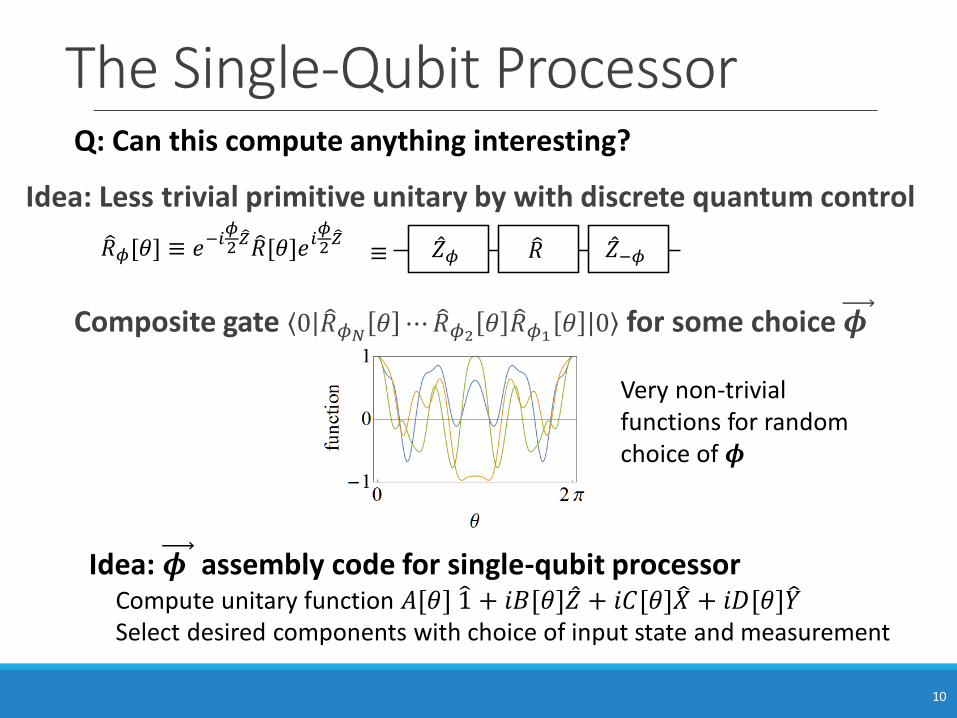
Idea: 𝝓 assembly code for single-qubit processorCompute unitary function 𝐴[𝜃] 1 + 𝑖𝐵[𝜃] መ𝑍 + 𝑖𝐶[𝜃] 𝑋 + 𝑖𝐷[𝜃] 𝑌Select desired components with choice of input state and measurement

Composite gate ۦ ȁ0 𝑅𝜙𝑁𝜃 ⋯ 𝑅𝜙2

𝜃 𝑅𝜙1𝜃 ȁ ۧ0 for some choice 𝝓

The Single-Qubit Processor

Idea: Less trivial primitive unitary by with discrete quantum control

10

𝑅𝜙[𝜃] ≡ 𝑒−𝑖𝜙2𝑍 𝑅[𝜃]𝑒𝑖

𝜙2𝑍 𝑅መ𝑍𝜙 መ𝑍−𝜙≡

Very non-trivial functions for random choice of 𝝓

Q: Can this compute anything interesting?

Qubit Unitary Function SynthesisQ: Why is this hard? Analogy:◦ Single-qubit gate synthesis from {H, T}

◦ Single-qubit function synthesis from { 𝑅𝜙 𝜃 , 𝝓 ∈ ℝ}

Exponential time for finding best-fit 𝝓 via gradient descent◦ 𝑅𝜙𝑁

𝜃 ⋯ 𝑅𝜙2𝜃 𝑅𝜙1

𝜃 = 𝐴 𝜃 1 + 𝑖𝐵 𝜃 መ𝑍 + 𝑖𝐶[𝜃] 𝑋 + 𝑖𝐷[𝜃] 𝑌

Necessary & sufficient constraints on achievable 𝑨 𝜽 , 𝑪[𝜽]1

1. 𝐴 0 = 1

2. 𝐴 𝜃 2 + 𝐶 𝜃 2 ≤ 1

3. 𝐴 𝜃 = σ𝑘=0𝑁/2

𝑎𝑘 cos 𝑘𝜃

4. 𝐶 𝜃 = σ𝑘=1𝑁/2

𝑐𝑘 sin(𝑘𝜃)

◦ Given 𝐴 𝜃 , 𝐶[𝜃], can compute 𝝓 in classical poly(N) time

Fourier series

1Low, Yoder, Chuang, Phys. Rev. X 6, 041067 (2016) 11

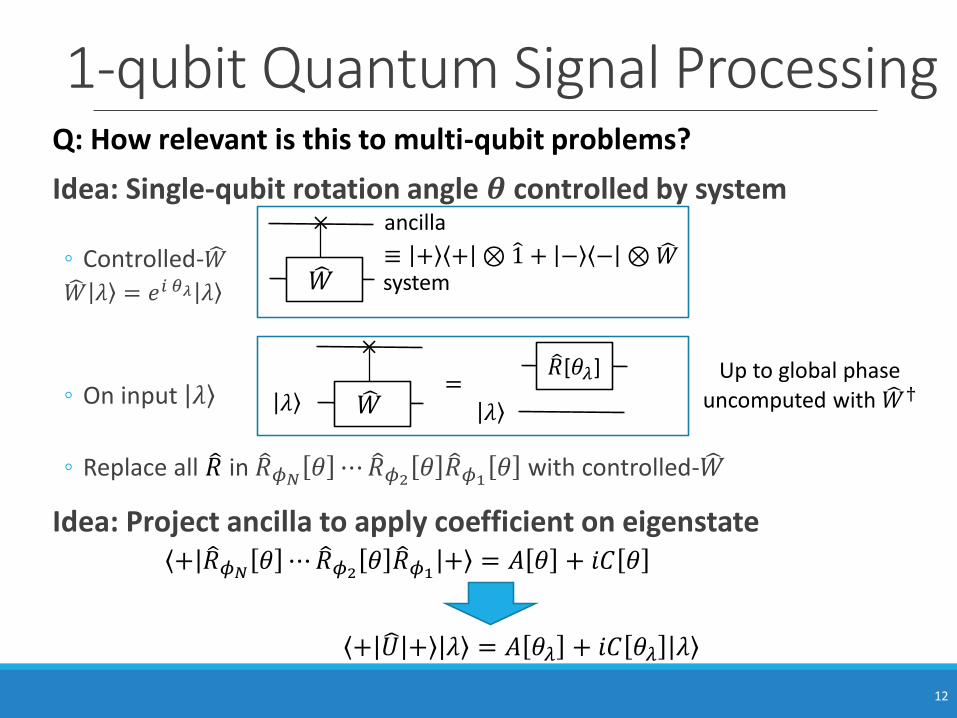
Idea: Single-qubit rotation angle 𝜽 controlled by system

◦ Controlled- 𝑊𝑊ȁ ۧ𝜆 = 𝑒𝑖 𝜃𝜆ȁ ۧ𝜆

◦ On input ȁ ۧ𝜆

◦ Replace all 𝑅 in 𝑅𝜙𝑁𝜃 ⋯ 𝑅𝜙2

𝜃 𝑅𝜙1𝜃 with controlled- 𝑊

Idea: Project ancilla to apply coefficient on eigenstate

1-qubit Quantum Signal Processing

𝑊

×

≡ ȁ ۧ+ ۦ ȁ+ ⊗ 1 + ȁ ۧ− ۦ ȁ− ⊗ 𝑊

12𝑊

×

=ȁ ۧ𝜆

𝑅[𝜃𝜆]

ȁ ۧ𝜆

Up to global phase uncomputed with 𝑊†

ۦ ȁ+ 𝑈ȁ ۧ+ ȁ ۧ𝜆 = 𝐴 𝜃𝜆 + 𝑖𝐶 𝜃𝜆 ȁ ۧ𝜆

ۦ ȁ+ 𝑅𝜙𝑁𝜃 ⋯ 𝑅𝜙2

𝜃 𝑅𝜙1ȁ ۧ+ = 𝐴 𝜃 + 𝑖𝐶 𝜃

12

ancilla

system

Q: How relevant is this to multi-qubit problems?

Quantum Signal Processing (cont.)

Approximate 𝑒𝑖 𝜃 → 𝑒𝑖 ℎ 𝜃 with degree N/2 Fourier series

◦ Input: Objective function ℎ: [0,2𝜋) → [0,2𝜋)

◦ 𝐴 𝜃 + 𝑖𝐶 𝜃 − 𝑒𝑖 ℎ 𝜃∞≤ 𝜖 ⇒ can find achievable 𝐴1 𝜃 + 𝑖𝐶1 𝜃 s.t.

𝐴1 𝜃 + 𝑖𝐶1 𝜃 − 𝑒𝑖 ℎ 𝜃∞≤ 8𝜖

Eigenphase transformation

◦ Output: ۦ ȁ+ 𝑈ȁ ۧ+ ȁ ۧ𝜆 = 𝐴1 𝜃𝜆 + 𝑖𝐶1 𝜃𝜆 ȁ ۧ𝜆 ≈ 𝑒𝑖 ℎ 𝜃𝜆 ȁ ۧ𝜆

◦ Query Complexity N vs. 𝜖 depends on smoothness / analyticity of 𝑒𝑖 ℎ 𝜃

◦ Trace distance ≤ 8𝜖

◦ Success probability ≥ 1 − 16𝜖

131Methodology of … Composite Quantum Gates, Low, Yoder, Chuang, Phys. Rev. X 6, 041067 (2016)

Q: What can this do?

k-smooth: 𝜖−1/𝑘

Analytic: log(1/ 𝜖)Entire: super-logarithmic

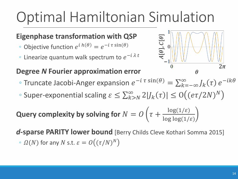
Optimal Hamiltonian SimulationEigenphase transformation with QSP

◦ Objective function 𝑒𝑖 ℎ 𝜃 = 𝑒−𝑖 𝜏 sin(𝜃)

◦ Linearize quantum walk spectrum to 𝑒−𝑖 𝜆 𝑡

Degree N Fourier approximation error

◦ Truncate Jacobi-Anger expansion 𝑒−𝑖 𝜏 sin(𝜃) = σ𝑘=−∞∞ 𝐽𝑘 𝜏 𝑒−𝑖𝑘𝜃

◦ Super-exponential scaling 휀 ≤ σ𝑘>𝑁∞ 2ȁ𝐽𝑘 𝜏 ȁ ≤ Ο (𝑒𝜏/2𝑁)𝑁

Query complexity by solving for 𝑁 = 𝑂 𝜏 +log(1/ )

log log(1/ )

d-sparse PARITY lower bound [Berry Childs Cleve Kothari Somma 2015]

◦ 𝛺(𝑁) for any 𝑁 s.t. 휀 = 𝛰 (𝜏/𝑁)𝑁

14

𝜃2𝜋

𝐴[𝜃],𝐶[𝜃]

Big Crunch Big Rip

15

Gate optimal simulation

Time-dependent simulation

Open quantum system simulation

Hamiltonians with structured information

Analog simulation [Stephen Piddock 2:00-2:40 !]

Other query models

Many open problems in Quantum simulation

3. Conclusion

Quantum Signal

Processor1

Quantum Control3

Quantum Algorithms2,5

Quantum

Metrology4

16

Thank you!

Work related to the single-qubit quantum signal processor1) Hamiltonian simulation by qubitization, Low, Chuang, arXiv preprint arXiv:1610.065462) Optimal Hamiltonian simulation by quantum signal processing, Low, Chuang, Physical Review Letters 118 (1), 0105013) Methodology of resonant equiangular composite quantum gates, Low, Yoder, Chuang, Physical Review X 6 (4), 0410674) Quantum imaging by coherent enhancement, Low, Yoder Chuang, Physical Review Letters 114 (10), 1008015) Fixed-point quantum search with an optimal number of queries , Yoder, Low, Chuang, Physical Review Letters 113 (21), 210501