optimal inventory control in cardboard box producing...
TRANSCRIPT

Optimal Inventory Control inCardboard Box Producing Factories:
A Case Study
Catherine D. Black
Thesis presented in partial fulfilment of the requirements for the degreeMaster of Science in Engineering Sciences at the Department of Applied
Mathematics of the University of Stellenbosch, South Africa
Supervisor: Prof J.H. van Vuuren July 2004


Declaration
I, the undersigned, hereby declare that the work contained in this thesis is my ownoriginal work and that I have not previously in its entirety or in part submitted it at anyuniversity for a degree.
Signature: Date:
i

ii
Abstract
This thesis is a case study in optimal inventory control, applied to Clickabox factory, aSouth African cardboard box producer from whom cardboard boxes may be ordered atshort notice via the internet.
The problem of developing a decision–support system for optimal stockholding at thefactory, in order to minimize cardboard off–cut wastage subject to required service levels,is addressed in this thesis. Previously a simple replenishment policy, based largely onexperience, was implemented at the factory. The inventory model developed for andapplied to Clickabox in this thesis takes account of a raw materials substitution cascade,as well as the stochasticity of demand, and other factors such as cost, service level andspatial requirements for the storage of stock. This combination of stochastic demand andproduct substitution has not, to the author’s knowledge, previously been dealt with inthe literature.
There are two primary deliverables of this study. The first is a suggestion as to the suitablestock composition (cardboard types from which boxes may be manufactured) to be keptin inventory at the factory. The second deliverable is a computerised decision–supportsystem, based on the inventory model developed, to aid in future inventory replenishmentdecisions at Clickabox.
Some of the results of this thesis have, at the time of writing, already been implementedwith success at the factory. These include the suggestions given to the managementof Clickabox as to the suitable stock types to be held in inventory, which have beenimplemented in stages since March 2003. The suggested stock composition has proven tobe superior to the previous stock types held, in terms of a reduction in off–cut wastageand increased availability of suitable boards.

iii
Opsomming
Hierdie tesis is ’n gevallestudie in optimale voorraadbeheer, toegepas op Clickabox fabriek,’n Suid–Afrikaanse kartondoosprodusent by wie kartondose op kort kennisgewing via dieinternet bestel kan word.
In hierdie tesis word ’n besluitnemingsteunstelsel ontwikkel vir optimale bestuur van voor-raad by die fabriek, wat karton afknipselvermorsing onderhewig aan vereiste diensvlakkeminimeer. Vantevore is ’n eenvoudige voorraad aanvullingstrategie, wat hoofsaaklik opondervinding gebaseer was, by die fabriek toegepas. ’n Wetenskaplike gefundeerde voor-raadmodel word vir Clickabox ontwikkel en toegepas, waarin ’n rou–voorraad kaskade–substitusie proses in aanmerking geneem word, asook die stogastiese vraag na kartondoseen faktore soos prys, diensvlakke en benodigde stoorruimte. Hierdie kombinasie van sto-gastiese vraag en rou–voorraad kaskade–substitusie is, tot die skrywer se kennis, nog niein die literatuur behandel nie.
Die studie het twee hoof–uitkomste ten doel. Die eerste is ’n aanbeveling ten opsigte van’n geskikte rou–voorraad samestelling (kartontipes waaruit kartondose geproduseer kanword) wat by die fabriek in voorraad gehou moet word. Die tweede is ’n rekenaarmatigebesluitnemingsteunstelsel, wat op die ontwikkelde voorraadbeheermodel gegrond is, enwat vir toekomstige besluite in verband met voorraadaanvulling by Clickabox bedoel is.
Van die resultate wat in hierdie tesis vervat is, is reeds ten tyde van die opskryf daarvandoeltreffend by die fabriek geımplementeer. Ondermeer is die aanbeveling in verbandmet die geskikte voorraadsamestelling, geleidelik vanaf Maart 2003 by die fabriek inge-faseer. Dit het duidelik geword dat hierdie samestelling beter as die vorige voorraad-profiel funksioneer, in terme van ’n verlaging in afknipselvermorsing en ’n verhoging indie beskikbaarheid van geskikte kartonne.

iv

v
Acknowledgements
The author hereby wishes to express her gratitude towards those without whose supportthe completion of this thesis would have been impossible:
• Prof Jan van Vuuren for his guidance, insight, patience and dedication, particularlygiven the difficulties of distance.
• The staff of Clickabox, and in particular Mr Piet Taljaard, for their enthusiasticsupport of the project, willingness to provide all the information required, andtolerance of my frequent presence at the factory.
• Mr Werner Grundlingh for his assistance with technical typesetting issues.
• T-Systems SA for their sponsorship of this research project.
• The Department of Applied Mathematics of the University of Stellenbosch, for theuse of their computing facilities.
• My husband, who bore the brunt of my frustrations along the way.

vi
Terms of Reference
This thesis is a case study in optimal inventory control at Clickabox, a cardboard boxmanufacturing company in the South African Western Cape Industria. The company’sinventory control practices take into account a number of factors, most notably non-stationary, partially observed stochastic demand and cascading product substitution. Tothe author’s knowledge this combination of factors has not previously been dealt with inthe literature.
The company was founded by Mr Bob Fuller in May 1988 as Corrucape Packaging CC,the first private carton manufacturing plant in the greater Cape Town area. Its turnovergrew steadily and reached a high point in 1996, when it achieved an annual turnover ofR4.3 million. It was converted to a PTY LTD company in 1997. Stiff competition andMr Fuller’s approach with respect to remaining a one–man business led to a decline inturnover in 1997 and 1998, and as a result he decided to sell the company. In October 1999the company was bought by Mr Piet Taljaard. The new directors, the Taljaard FamilyTrust, changed the company name to Clickabox Pty Ltd in November 2000, reflecting thecompany’s new focus on e–commerce.
The need for a scientific inventory control process was identified during the developmentof a web–based interface for Clickabox that allows customers to receive quotes and placeorders online. This website interfaces with the Pastel [58] accounting system, used byClickabox, that maintains information on stock levels, sales, etc. It was developed duringthe period October 2000 – August 2001 by Netcommerce Consulting [69], a companyowned and managed by Mr Leon Swanepoel.
Mr Swanepoel introduced Mr Taljaard, the director of Clickabox factory, to Prof Jan vanVuuren from the Department of Applied Mathematics at the University of Stellenbosch,in March 2001. At this meeting Mr Taljaard expressed his interest in a solution to hisinventory control problem. Since then, the factory has twice been used as a case studyfor projects forming part of a project driven postgraduate course at the Department ofApplied Mathematics, called Methods of Operations Research [25]. This thesis is the firststudy beyond Honours level to be conducted at Clickabox.
Prof van Vuuren was the supervisor for this thesis. The first meeting between the authorand the director of Clickabox took place on 8 May 2001, and after a number of subsequentvisits a research proposal was drawn up and presented to the director. The factory wasvisited by the author on a weekly basis during the two months July to August 2001, forthe purposes of observing the quoting, ordering, manufacturing, and other administrativeprocesses. Subsequent to that period, the factory was visited by the author whenever

vii
required, but in any case at least on a bi–monthly basis. The computing facilities ofthe Department of Applied Mathematics, as well as private facilities, were used duringnumerical simulations so as to obtain model solutions. Much of the data required werecollected by the author on site at the factory, or provided by correspondence with MrTaljaard. Mr Jannie Brandt, a programmer from Netcommerce Consulting, assisted withextraction of data from the Pastel database. Work on this thesis was completed in July2004, and work emanating from this study was presented twice at annual conferences ofthe Operations Research Society of South Africa (ORSSA).

viii
Definition of Symbols
A number of symbols will conform to the following convention:A Symbol denoting a set. (Caligraphy capitals)A Symbol denoting a matrix. (Boldfaced capitals)a Symbol denoting a vector. (Underlined letters)
α(β) Service level of board βAt Total floor area at Clickabox factory [m2]As Floor area of the storage space at Clickabox factory [m2]A(β) Area of board type β [m2]β Fraction of demand that is backordered during a stockout periodB Set of indices of board types kept in inventory, |B| = b and
B = BAC ∪ BDWB
BAC Set of indices of board types of cardboard type AC kept in inventory,|BAC | = 28
BDWB Set of indices of board types of cardboard type DWB kept in inventory,|BDWB| = 18
χnj The sum of n independent, identically distributed random variables with
distribution rvi
j,z in class j ∈ Kc Cost of capital rate [Rands per week]D(β) Average annual demand for board type β [Sheets per annum]d
vit Demand class of board preference vector vi in week t
Φ(ξ) The probability density function of random demand ξφi,f The wastage cost incurred when the f–th board in board preference vector
vi is used instead of the optimal board [Rands per board]fn(x) Discounted expected cost for an n–period model under an optimal control
policy with an on hand inventory level of x [Rands per week]Ft(ft)(j, x) Expected holding cost in time period t, given demand state j and inventory
level x [Rands per time period]G Set of grid points (potential stock boards)gi,β The wastage per board when one sheet of type i ∈ S is cut out of a board
of type β ∈ B [m2]g′
i,β The percentage wastage when one sheet of type i ∈ S is cut out of a boardof type β ∈ B
G(β)t (u
(β)t ) The single week expected cost for board type β and inventory
position ut [Rands per week]

ix
η$(z) Spatial constraint for cardboard type z of rank $ [Number of boards]
h′ The height to which boards may be stacked [m]h(β) Holding cost per week of board type β [Rands per week]hT Total holding cost per week over all board types [Rands per week]
H(β)t (u
(β)t ) The total single week cost for board type β and inventory position ut,
comprising the purchasing cost and the inventory cost Gt(ut|πt, l)[Rands per week]
Ivit Vector of information available at the start of week t for board
preference vector vi
κ(β) Number of order cycles in a year for board type β
Kjt The fixed order cost in week t and demand state j [Rands per order]
Kj
t The expected fixed order cost in week t + 1 and demand state j [Rands perorder]
K Set of indices of demand classes, |K| = 7L(S, x) Expected period cost for on hand inventory level x and order–up–to level SLBf
The length of entry f in the set B [m]LGf
The length of entry f in the set G [m]LOf
The length of entry f in the set O [m]l Lead–time for delivery of raw materials [Number of weeks]
m(i,β)t The maximum number of sheets, optimally produced by board preference
vector vi, i ∈ V, that can be produced from board type β ∈ B in week t[Sheets per board]
m(β,f) The maximum number of sheets of type f ∈ S that can be produced fromboard type β ∈ B [Sheets per board]
nj(σvi) The number of times that state j occurs in the sequence σvi
Oi Modified set of past orders (excluding those made by β1 to βi)O Set indices of past ordersΠ
vi
j,t The probability of board preference vector vi being in demand statej, given the information available up to week t
Pvi The transition probability matrix for board preference vector vi
Pvi
j,k The probability of the demand state of board preference vector vi changing
from state j to state kp(β) Purchasing cost per unit of board type β [Rands per board]
q(β)t The quantity of board type β ordered in week t [Boards per week]
q∗ Economic order quantity [Number of boards]Rc Rental cost per volume of stock per week [Rands per m3 per week]Rp Total annual rent paid [Rands per annum]Rs Proportion of annual rent paid attributed to storage space [Rands per annum]RT Total rent per period [Rands per week]r Re–order level [Number of boards]rvi Probability distribution of demand for board preference vector vi
rvi
j,k Probability of a demand realisation in demand class k, given a current
demand state of j distribution of demand for board preference vector vi
rvi
j,k The probability distribution of the lead time demand of board preference
vector vi

x
S Set of indices of possible sheet types for which orders may be received, |S| = sS Order–up–to or base–stock level [Number of boards]S∗(β) Optimal number of stockouts of board type β in a year [Stockouts per annum]
S(β)
Probability of a stockout of board type β in each order cycles Re–order level [Number of boards]s(β) Cascading shortage cost per unit of board type β [Rands per board]T Point of time at which the myopic behaviour of the demand is terminatedT Set of indices of one–week time periods, |T | = 52τ Expediting factorθ Discount factor
u(β)t Inventory position of board type β at the start of week t [Number of boards]
υvi
j Mean of distribution j
υ(2)vi
j Second moment about the mean of distribution j
v(β) Volume of board β [m3]V Set of indices of board preference vectors, |V| = µvi Board preference vector iWBf
The width of entry f in the set B [m]WGf
The width of entry f in the set G [m]WOf
The width of entry f in the set O [m]w
vit Realised demand for board preference vector vi in week t [Number of boards]
W βt Realised demand for board type β in week t [Number of boards]
W βt,i The i–th level demand for board type β in week t [Number of boards]
W βt Realised demand for board type β during the lead time from week t
[Number of boards]Ψ(β) Shortage cost of board type β [Rands per week]X Set of indices of boards in the board preference vector, |X | = 3
x(β)t Inventory level of board type β in week t [Number of boards]
ζ(i,k)t The set of all possible demand state sequences σ
vit = (d
vit , d
vi
t+1, . . . dvi
t+l)such that d
vit = k

xi
Glossary
Adaptive policy. A policy in which the information gained during each time period isused to update the estimates of unknown parameters, for use during the subsequentperiods.
Backorder. A customer demand that has not been met due to a stockout situation,where the customer is prepared to wait for the raw materials to arrive in stock.
Base–stock level. The inventory level to which an inventory replenishment order shouldbring the stock on hand.
Base–stock Policy A continuous review inventory replenishment policy which com-prises a single parameter, namely an order–up–to or base–stock level, S.
Bill of Materials. A listing of raw materials required by a manufacturer to completeor produce a specified product.
Board. A piece of cardboard received as is from a supplier, not yet cut to the correctdimensions for the manufacturing of a cardboard box.
Board Preference Vector. A set of three boards from which a sheet order may beproduced, listed in order of increasing offcut wastage incurred.
Certainty equivalent control. Inventory replenishment policies under which somedata are observed, the unknown parameters are estimated by maximum likelihoodmethods, and inventory policies are chosen, assuming that the demand distributionparameters equal the estimated values.
Cost of capital rate. The cost of financing an investment, such as the interest paid ona loan.
Continuous review. An inventory control policy under which replenishment ordersmay be placed at any time.
Decision Support System. A computerised system designed to assist managers in se-lecting and evaluating courses of action, by providing a logical analysis of the rele-vant factors influencing decisions.
Economic Order Quantity. The optimal replenishment order quantity that minimizesthe holding and order costs of on hand inventory.

xii
Fill Rate. The percentage of inventory items demanded during a fixed time period thatwill be in stock when needed.
Holding cost. The cost per unit of holding stock in inventory. This comprises rental
cost, insurance, and the opportunity cost of tied–up capital investment.
Inventory level. On hand inventory less backorders.
Inventory position. On hand inventory together with stock on order from raw mate-
rials suppliers, less backorders.
ISO9000. Certification Standards created by the International Organization for Stan-dardizations in 1987 that now play a major role in setting process documentationstandards for global manufacturers. These standards are recognized in over 100countries. ISO9000 provides general requirements for various aspects of a firm’s op-erations, including Purchasing, Design Controls, Contracts, Inspection, Calibration,etc. [2].
K–convexity. A condition used to prove the optimality of the (s, S) policy in the caseof both fixed and variable order costs. A function is said to be K–convex if thesecant line connecting any two points on the graph of the function, when extendedto the right, is never more than K units above the function.
Lead Time. The time span between the placing of a replenishment order and its sub-sequent arrival into inventory.
Lost Sales. Potential sales that are lost, because there is no stock available in inventory(if the waiting time for delivery of an order is too long).
Manufacturer. A company involved in a series of interrelated activities and operationsinvolving the design, material selection, planning, production, quality assuranceand marketing of commercial goods.
Moving Average. The average over the last N points in a set of data is said to be an“N–period moving average.” This is sometimes used to make forecasts, based onthe most recent data.
Myopic Policy. A policy which does not take future costs as a result of current decisionsinto account.
Non–stationary Demand. Demand having a probability distribution that changesover time.
Obsolescence. Stock that is no longer usable for its intended purpose through expira-tion, contamination, damage, or change of need.
Offcut Wastage. The wastage incurred when boards are cut into sheets of the requireddimension in order to produce cardboard boxes, resulting in pieces of cardboardtoo small for re–use.
On hand inventory. The stock immediately available in inventory.

xiii
Opportunity cost. Potential earnings from an alternative investment, such as the in-terest which would be earned on capital were it to be placed in a bank account,instead of being invested in inventory.
Order cost. The costs involved in placing an inventory replenishment order at a supplier.
Order cycle. The length of time between the placement of successive orders to replenishan inventory.
Order quantity. The number of stock items to be ordered when an inventory replen-ishment order is placed.
Order–up–to level The on hand inventory level up to which a replenishment ordershould bring the stock on hand in an (s, S)–model or under a base–stock policy.
Pallet. A rectangular wooden based support for unitized lots of cardboard, subject tostandards of length and width for storage in pre–determined places. Constructionof the wooden base is such that there is air space between the bottom of the palletand the load bearing surface of the pallet sufficient to allow the insertion of liftingforks so as to transport the pallet by forklift.
Partially Observed Demand. Demand for which the underlying distribution is notcompletely observed — it is only partially observed through the demand that hasactually realised.
Periodic Review System. An inventory replenishment or control policy in which theorder cycle is a fixed period of time.
Product Substitution. The use of a non–primary or sub–optimal product or compo-nent (at a cost), normally when the primary or optimal item is not available.
Purchasing cost. The cost per unit of raw materials purchased from a supplier.
(Q, r) Model. An inventory replenishment or control policy in which an order of mag-nitude Q inventory units is placed if the inventory level reaches the re–order level
r.
Raw materials. Materials purchased by a manufacturer to be used in the manufactur-ing of products.
Recyclable Materials. Goods that may be collected for re–use as raw materials tomanufacture new products.
Rental cost. The cost of hiring space used for warehouse and inventory control func-tions, including office space. For owned buildings a fair market rental value ordepreciation is used instead.
Re–order level. The inventory level at or below which a purchase requisition is initi-ated. It is a combination of expected usage during the lead time period and a safety
stock buffer.

xiv
Re–order Quantity. The number of stock items to be ordered when a re–order level isreached.
Safety stock. Inventory which serves to promote continuous supply when unpredictabledemands exceed forecasts, or the delivery of raw materials from a supplier is de-layed.
Scrap Material. Material that is deemed worthless to a production facility and is onlyvaluable to the extent to which it can be recycled.
Service Level. The probability of not running short of stock before an inventory replen-ishment order arrives (i.e., the percentage of order cycles during the year in whichthere were no stockouts).
Set–up Cost. The marginal cost of a machine or workstation setup. This generallyincludes the labour and the materials cost associated with the scrap material gen-erated by the setup.
Sheet. A piece of cardboard that has been cut to the exact dimensions required for themanufacturing of a cardboard box order.
Shortage cost. The cost incurred when a sub–optimal inventory item must be used toproduce an order, due to a stockout of the optimal inventory item.
Simulation. A representation of reality, often used for experimentation. In operationsmanagement, computer simulations of complex systems, such as factories or serviceprocesses, are often utilized in to order experiment with changes in managementdecisions. Experimenting with a simulation model may help to identify problemsand opportunities for improvement, without having to actually build (or change) thephysical system in order to evaluate the repercussions of such changes. Computersimulations of this type are generally discrete event simulation models, as opposedto continuous simulation models in which quantities have continuous measure.
(s, S) Model. An inventory replenishment or control policy in which an order is placedif the inventory level is less than or equal to some specified value, s. The size ofthe order placed is sufficient to raise the inventory level to the order–to level S.
Stationary Demand. Demand having a single probability distribution that does notchange over time.
Stock. The commodity or commodities on hand in a storeroom or warehouse to supportoperations.
Stockout. The condition existing when a supply requisition cannot be filled from stock.
Supplier. A provider of raw materials.

Table of Contents
List of Figures xix
List of Tables xxi
1 Introduction 1
1.1 Introduction to Clickabox Factory . . . . . . . . . . . . . . . . . . . . . . 1
1.1.1 Products and Services . . . . . . . . . . . . . . . . . . . . . . . . 2
1.1.2 The Industry as a Whole . . . . . . . . . . . . . . . . . . . . . . . 2
1.2 Informal Problem Description . . . . . . . . . . . . . . . . . . . . . . . . 3
1.3 Thesis Overview . . . . . . . . . . . . . . . . . . . . . . . . . . . . . . . . 3
2 Literature Review 5
2.1 Brief Overview of Inventory Theory . . . . . . . . . . . . . . . . . . . . . 5
2.1.1 Stationary Demand, Fully Observed . . . . . . . . . . . . . . . . . 8
2.1.2 Non–stationary Demand, Fully Observed . . . . . . . . . . . . . . 8
2.1.3 Stationary Demand, Partially Observed . . . . . . . . . . . . . . . 11
2.1.4 Non–stationary Demand, Partially Observed . . . . . . . . . . . . 13
2.2 Important Concepts in Inventory Modelling . . . . . . . . . . . . . . . . 14
2.2.1 Modelling of a Markovian Decision Process . . . . . . . . . . . . 14
2.2.2 Multiple Products and Stock Substitution . . . . . . . . . . . . . 15
2.2.3 Stockout Situations . . . . . . . . . . . . . . . . . . . . . . . . . . 16
2.2.4 Variability of Lead Time . . . . . . . . . . . . . . . . . . . . . . . 17
2.2.5 Advance Demand Information . . . . . . . . . . . . . . . . . . . . 17
2.3 Chapter Summary . . . . . . . . . . . . . . . . . . . . . . . . . . . . . . 18
3 Clickabox Factory 19
3.1 Clickabox : The Business . . . . . . . . . . . . . . . . . . . . . . . . . . . 20
xv

xvi Table of Contents
3.1.1 Business Objectives . . . . . . . . . . . . . . . . . . . . . . . . . . 20
3.1.2 Business Strategy . . . . . . . . . . . . . . . . . . . . . . . . . . . 21
3.1.3 Financial Situation . . . . . . . . . . . . . . . . . . . . . . . . . . 22
3.2 Clickabox : The Factory . . . . . . . . . . . . . . . . . . . . . . . . . . . . 22
3.2.1 Factory Location and Layout . . . . . . . . . . . . . . . . . . . . 23
3.2.2 Workshop Machinery and Manufacturing Process . . . . . . . . . 26
3.2.3 Factory Staff . . . . . . . . . . . . . . . . . . . . . . . . . . . . . 28
3.3 Raw Materials . . . . . . . . . . . . . . . . . . . . . . . . . . . . . . . . . 28
3.4 Order Classification . . . . . . . . . . . . . . . . . . . . . . . . . . . . . . 30
3.5 Processes at Clickabox . . . . . . . . . . . . . . . . . . . . . . . . . . . . 32
3.5.1 Ordering of Stock from Raw Materials Suppliers . . . . . . . . . . 33
3.5.2 Ordering of Boxes from Clickabox by clients . . . . . . . . . . . . 33
3.5.3 Manufacturing Process Protocol . . . . . . . . . . . . . . . . . . . 38
3.5.4 Administrative Manufacturing Process . . . . . . . . . . . . . . . 39
3.5.5 Post Manufacturing Process . . . . . . . . . . . . . . . . . . . . . 40
3.6 Chapter Summary . . . . . . . . . . . . . . . . . . . . . . . . . . . . . . 40
4 Analysis of Board Demand 41
4.1 Description of Demand Data . . . . . . . . . . . . . . . . . . . . . . . . 41
4.2 Determining Suggested Stock Board Profile . . . . . . . . . . . . . . . . . 43
4.2.1 ABC Analysis of Cardboard Types . . . . . . . . . . . . . . . . . 43
4.2.2 Graphical Representation of Data . . . . . . . . . . . . . . . . . . 45
4.2.3 Restrictions on Stock Boards . . . . . . . . . . . . . . . . . . . . 47
4.2.4 Heuristic for Determining a Suggested Stock Profile . . . . . . . 47
4.2.5 Results . . . . . . . . . . . . . . . . . . . . . . . . . . . . . . . . 50
4.2.6 Evaluation of Results . . . . . . . . . . . . . . . . . . . . . . . . . 54
4.3 Demand Distributions . . . . . . . . . . . . . . . . . . . . . . . . . . . . 54
4.3.1 Board Preference Vectors . . . . . . . . . . . . . . . . . . . . . . 54
4.3.2 Board Demands . . . . . . . . . . . . . . . . . . . . . . . . . . . 56
4.4 Chapter Summary . . . . . . . . . . . . . . . . . . . . . . . . . . . . . . 63
5 Inventory Model 67
5.1 General Modelling Assumptions . . . . . . . . . . . . . . . . . . . . . . . 67
5.2 Spatial Constraints . . . . . . . . . . . . . . . . . . . . . . . . . . . . . . 68

Table of Contents xvii
5.3 Board Holding costs . . . . . . . . . . . . . . . . . . . . . . . . . . . . . 70
5.3.1 Rental Cost . . . . . . . . . . . . . . . . . . . . . . . . . . . . . . 70
5.3.2 Opportunity Cost . . . . . . . . . . . . . . . . . . . . . . . . . . . 71
5.3.3 Insurance Cost . . . . . . . . . . . . . . . . . . . . . . . . . . . . 72
5.3.4 Total Holding Costs . . . . . . . . . . . . . . . . . . . . . . . . . 72
5.4 Cascading Shortage Costs . . . . . . . . . . . . . . . . . . . . . . . . . . 72
5.5 Service Level Measures . . . . . . . . . . . . . . . . . . . . . . . . . . . . 73
5.6 Optimal Control Policy . . . . . . . . . . . . . . . . . . . . . . . . . . . . 77
5.6.1 Board Preference Vector Demand . . . . . . . . . . . . . . . . . . 78
5.6.2 Inventory Position . . . . . . . . . . . . . . . . . . . . . . . . . . 79
5.6.3 Shortage Cost Revisited . . . . . . . . . . . . . . . . . . . . . . . 85
5.6.4 Optimal Inventory Policy . . . . . . . . . . . . . . . . . . . . . . . 86
5.7 Sub–optimal Control Policy . . . . . . . . . . . . . . . . . . . . . . . . . 88
5.8 Chapter Summary . . . . . . . . . . . . . . . . . . . . . . . . . . . . . . 90
6 Model Results 91
6.1 Structure of the Simulation Model . . . . . . . . . . . . . . . . . . . . . . 91
6.1.1 Decision Support System Interface . . . . . . . . . . . . . . . . . 92
6.1.2 Simulation Database . . . . . . . . . . . . . . . . . . . . . . . . . 92
6.1.3 Program Code . . . . . . . . . . . . . . . . . . . . . . . . . . . . . 92
6.1.4 Decision Support System Output . . . . . . . . . . . . . . . . . . 93
6.2 Model Validation . . . . . . . . . . . . . . . . . . . . . . . . . . . . . . . 94
6.2.1 Continuity . . . . . . . . . . . . . . . . . . . . . . . . . . . . . . . 95
6.2.2 Consistency . . . . . . . . . . . . . . . . . . . . . . . . . . . . . . 95
6.2.3 Degeneracy . . . . . . . . . . . . . . . . . . . . . . . . . . . . . . 98
6.2.4 Absurd Conditions . . . . . . . . . . . . . . . . . . . . . . . . . . 98
6.3 Determination of Simulation Truncation Point . . . . . . . . . . . . . . . 99
6.4 Single Period Optimisation Results . . . . . . . . . . . . . . . . . . . . . 100
6.5 Multiple Period Optimisation Results . . . . . . . . . . . . . . . . . . . . 101
6.6 Evaluation of Results . . . . . . . . . . . . . . . . . . . . . . . . . . . . . 102
6.7 Chapter Summary . . . . . . . . . . . . . . . . . . . . . . . . . . . . . . 104
7 Conclusion 105
7.1 Summary of What Has Been Achieved . . . . . . . . . . . . . . . . . . . 105

xviii Table of Contents
7.2 Further Work . . . . . . . . . . . . . . . . . . . . . . . . . . . . . . . . . 107
A Suggested Stock Boards 109
B Realised Demand and Shortage Cost 111
C Program Code 115
C.1 Determination of an Optimal Stock Profile . . . . . . . . . . . . . . . . . 116
C.2 Determination of the Sub–optimal Board Types . . . . . . . . . . . . . . 120
C.3 Calculation of the Optimal Board to use for a Sheet Order . . . . . . . . 121
C.4 Calculation of Transition Probabilities . . . . . . . . . . . . . . . . . . . 124
C.5 Calculation of Board Factor Probabilities . . . . . . . . . . . . . . . . . 125
C.6 Implementation of the Inventory Model . . . . . . . . . . . . . . . . . . 126
D Snapshot of Demand Data 141
E Board Preference Vectors 143
F Multiple Period Optimisation Results 151
G Instructions for using Compact Disc 153
References 155

List of Figures
2.1 Economic Order Quantity . . . . . . . . . . . . . . . . . . . . . . . . . . 6
2.2 Stock Movement Over Time under the (s, S) Inventory Policy . . . . . . 7
2.3 Stock Movement Over Time under the Base–Stock Inventory Policy . . . 9
2.4 Stock Movement Over Time under the (Q, r) Inventory Policy . . . . . . 17
3.1 View of Clickabox from Parin Street . . . . . . . . . . . . . . . . . . . . . 19
3.2 Turnover of Clickabox . . . . . . . . . . . . . . . . . . . . . . . . . . . . 21
3.3 Location of Clickabox . . . . . . . . . . . . . . . . . . . . . . . . . . . . . 22
3.4 Factory Layout . . . . . . . . . . . . . . . . . . . . . . . . . . . . . . . . 23
3.5 Storerooms and Office Area . . . . . . . . . . . . . . . . . . . . . . . . . 24
3.6 Production Area . . . . . . . . . . . . . . . . . . . . . . . . . . . . . . . 25
3.7 Machinery for Small Order Batches . . . . . . . . . . . . . . . . . . . . . 26
3.8 Machinery for Large Order Batches . . . . . . . . . . . . . . . . . . . . . 27
3.9 Forklift and Delivery Vehicle . . . . . . . . . . . . . . . . . . . . . . . . . 28
3.10 Manufacturing Process Flow Diagram . . . . . . . . . . . . . . . . . . . . 29
3.11 Raw Materials Delivery . . . . . . . . . . . . . . . . . . . . . . . . . . . . 30
3.12 Profiles of Cardboard Types Kept in Inventory at Clickabox . . . . . . . 30
3.13 The Regular Slotted Carton Box Type . . . . . . . . . . . . . . . . . . . 34
3.14 The Tuck–in–Flap Box Style . . . . . . . . . . . . . . . . . . . . . . . . . 34
3.15 Clickabox Website Order Screen . . . . . . . . . . . . . . . . . . . . . . . 35
3.16 Creasing Allowances . . . . . . . . . . . . . . . . . . . . . . . . . . . . . 36
3.17 Clickabox Website Quotation Screen: Buy–in Board . . . . . . . . . . . . 37
3.18 Clickabox Website Quotation Screen: Stock Board . . . . . . . . . . . . . 38
3.19 Bill of Materials . . . . . . . . . . . . . . . . . . . . . . . . . . . . . . . . 39
4.1 Example of a Works Ticket . . . . . . . . . . . . . . . . . . . . . . . . . . 42
xix

xx List of Figures
4.2 Cumulative Usage Values Stock in ABC Classification . . . . . . . . . . . 44
4.3 Graphical Representation of ABC Stock Classification . . . . . . . . . . . 45
4.4 Scatter Charts of Board Demand . . . . . . . . . . . . . . . . . . . . . . 46
4.5 Process of Finding the Suggested Stock Boards . . . . . . . . . . . . . . 49
4.6 Previous versus Proposed AC Stock against Sheet Orders . . . . . . . . . 50
4.7 Previous versus Proposed DWB Stock against Sheet Orders . . . . . . . 52
4.8 Demand Quantities of Board Preference Vector 1 . . . . . . . . . . . . . 57
4.9 Demand Quantities of Board Preference Vector 29 . . . . . . . . . . . . . 58
4.10 Graphical Depiction of Summary Statistics for each Demand Class . . . . 64
4.11 The Demand Realisation Distributions for Classes 2 to 6 . . . . . . . . . 65
4.12 The Demand Realisation Distributions for Class 7 . . . . . . . . . . . . . 65
6.1 Decision Support System Initial Option Screen . . . . . . . . . . . . . . . 92
6.2 Stages of the Single Period Optimisation Simulation . . . . . . . . . . . . 93
6.3 Stages of the Multiple Period Optimisation Simulation . . . . . . . . . . 93
6.4 Decision Support System Output Screen: Single Period Optimisation . . 94
6.5 Decision Support System Output Screen: Dynamic Optimisation . . . . . 94
6.6 Continuity of the Simulation Model . . . . . . . . . . . . . . . . . . . . . 96
6.7 Consistency of the Simulation Model . . . . . . . . . . . . . . . . . . . . 97
6.8 Non–degeneracy of the Simulation Model . . . . . . . . . . . . . . . . . . 98
6.9 Determination of the Simulation Transient Phase Truncation Point . . . 100
6.10 Suggested Dynamic Weekly Replenishment Parameters . . . . . . . . . . 103
C.1 Structure of the Database Tables . . . . . . . . . . . . . . . . . . . . . . 140

List of Tables
3.1 Cardboard Flute Types . . . . . . . . . . . . . . . . . . . . . . . . . . . . 31
3.2 Standard Orders . . . . . . . . . . . . . . . . . . . . . . . . . . . . . . . 31
3.3 Standard Stock . . . . . . . . . . . . . . . . . . . . . . . . . . . . . . . . 32
3.4 Cardboard Creasing Allowances . . . . . . . . . . . . . . . . . . . . . . . 36
4.1 Cardboard Type Classifications . . . . . . . . . . . . . . . . . . . . . . . 45
4.2 Current and Proposed AC Stock Board Profiles . . . . . . . . . . . . . . 51
4.3 Current and Proposed DWB Stock Board Profiles . . . . . . . . . . . . . 53
4.4 Example of a Board Preference Vector . . . . . . . . . . . . . . . . . . . 55
4.5 Results of the Distribution Analysis . . . . . . . . . . . . . . . . . . . . . 57
4.6 Frequency of Occurrence of Order Quantities . . . . . . . . . . . . . . . . 59
4.7 Summary Statistics of the Demand Classes . . . . . . . . . . . . . . . . . 60
4.8 Transitional Probabilities . . . . . . . . . . . . . . . . . . . . . . . . . . . 61
4.9 Example of Board Factors . . . . . . . . . . . . . . . . . . . . . . . . . . 62
5.1 Spatial Constraints . . . . . . . . . . . . . . . . . . . . . . . . . . . . . . 69
5.2 Theoretical Service Levels for AC Boards . . . . . . . . . . . . . . . . . . 76
5.3 Theoretical Service Levels for DWB Boards . . . . . . . . . . . . . . . . 77
5.4 Performance Measures . . . . . . . . . . . . . . . . . . . . . . . . . . . . 77
5.5 Calculation of Realised Demand: An Example . . . . . . . . . . . . . . . 84
5.6 Shortage Costs for an Example of the Calculation of Realised Demand . 84
5.7 Results of Trend and Correlation Anaylsis . . . . . . . . . . . . . . . . . 89
6.1 Results of Single Period Optimisation . . . . . . . . . . . . . . . . . . . . 101
6.2 Results of Multiple Period Optimisation . . . . . . . . . . . . . . . . . . 102
A.1 Sub–optimal Board Types for AC Stock Boards . . . . . . . . . . . . . . 109
xxi

xxii List of Tables
A.2 Sub–optimal Board Types for DWB Stock Boards . . . . . . . . . . . . . 110
D.1 Snapshot of Demand Date . . . . . . . . . . . . . . . . . . . . . . . . . . 141
E.1 AC Board Preference Vectors . . . . . . . . . . . . . . . . . . . . . . . . 143
E.2 DWB Board Preference Vectors . . . . . . . . . . . . . . . . . . . . . . . 147
F.1 Multiple Period Optimisation Results: AC Cardboard Types . . . . . . . 151
F.2 Multiple Period Optimisation Results: DWB Cardboard Types . . . . . . 152

Chapter 1
Introduction
Inventory is held by manufacturing companies for a number of reasons, such as to allow forflexible production schedules and to take advantage of economies of scale when orderingstock [55]. Most importantly, an inventory acts as a buffer between supply and demand,compensating for variations in demand and safeguarding against variations in deliverylead time of raw materials. Failure to meet demand compromises customer satisfaction,and may lead to high costs of emergency production [79]. The efficient managementof inventory systems is therefore a crucial element in the operation of any productioncompany [19]. Benefits from efficient inventory management to the customers include in-creased “off the shelf” availability of products, whilst benefits to the management includereduced tied–up investment capital in the inventory, reduced operating costs associatedwith warehousing functions, and a reduction in obsolescence accrual [35].
There are a number of factors that should be taken into account when developing aninventory model, such as the nature of the demand for the product, customer require-ments and costs involved. In this thesis, an inventory control model will be developed for amanufacturing company where the production process is characterised by non–stationary,partially observed stochastic demand and a cascade of stock substitution during produc-tion.
The remainder of this chapter is structured as follows: Clickabox, the factory on whichthe case study for this thesis is based, is introduced in §1.1, and a brief and informaldescription of the research problem to be considered in this thesis is given in §1.2. Finally,an overview of the structure of the remaining chapters in the thesis is given in §1.3.
1.1 Introduction to Clickabox Factory
Clickabox is a cardboard box manufacturer in the South African Western Cape. It is aprivately owned factory which caters for a niche in the local cardboard packaging industrycharacterised by short delivery times, and therefore availability of stock is a high priorityfor the company.
1

2 CHAPTER 1. INTRODUCTION
1.1.1 Products and Services
Clickabox has become an established manufacturer and supplier of cardboard boxes toindustries in the Western Cape. Its products include cartons (printed with either oneor two colours), creased boards, pads and sheets – all manufactured from corrugatedcardboard bought in from a number of large manufacturers, such as Mondi [52], Nampak
[56], and Atlantic packaging [5], who typically have long delivery response times for orders.
The company’s focus is on the manufacturing of smaller order quantities and deliveringwith a shorter response time than its competitors. This is the perceived gap left in themarket by the larger players mentioned above, and it is within this niche that Clickabox
competes.
The activities of Clickabox are divided into two kinds of business: long orders and quick
orders. Customers who are prepared to wait for up to ten working days for their ordersto be met may place a long order. Boxes ordered as such are less expensive, as partiallyprocessed boards are bought in from the supplier (whose lead time is ten days) at noextra cost to Clickabox and cut to size, so that offcut wastage is minimal. The company’sfocus is, however, on the market for quick orders. For these orders, produced from theunprocessed boards kept in stock at the factory, Clickabox guarantees product deliverywithin two working days. This is significantly faster than deliveries made by largercompanies, which may take up to three weeks to deliver an order to individuals. Theclosest competitor to Clickabox, in terms of delivery time, is Cape Town Box [14], whichguarantees a four day lead time [71].
Boxes are made to order; even very small orders are accepted by Clickabox, and freedelivery is offered on large orders. A major part of the service delivery of Clickabox is itsability to supply quick quotes to customers, and its ability to perform all the transactionsaccurately and quickly, in electronic fashion. The company website [57], from which itderives its name, forms a significant part of its service offering in this regard. Customersmay register, request quotes, and view inventory and product information online. Thewebsite gives the company a competitive advantage in that it makes its products accessibleto inexperienced clients.
1.1.2 The Industry as a Whole
The South African corrugated packaging industy is very competitive and has undergonea rationalisation phase during the period 1999–2001 [72]. Major players in the industry,like Mondi [52] and Kohler [41], have rationalised their capacity and have closed some oftheir production plants. Other companies, like Corruboard, Smart Packaging and Naledi,have closed down completely. With steeply rising input costs (due to price increases in thepaper industry) and a slump in the fruit exports from the South African Western Capeduring the period 2000–2001 [46], the capacity still exceeds the demand and there arevery few new entrants in the market. This abundance of competition heightens the needfor Clickabox to remain competitive in its pricing. Direct competitors include Cape Town
Box [14], Boxes for Africa [13], and a host of smaller manufacturers. This cut–throatcompetitiveness necessitates streamlining of all processes if companies wish to survive.

1.2. Informal Problem Description 3
1.2 Informal Problem Description
The goal of this study is to establish a good inventory management policy for Clickabox
factory.
The service offering of Clickabox, namely delivery of quick orders within two workingdays, is dependent on the availability of suitable cardboard in stock. Suitability of astock board is determined by the amount of off–cut wastage that results when it is usedto meet an order, which, in turn, depends on the dimensions of orders for boxes. Theobjective of the model in this thesis will be to minimize stockholding costs, subject tothe following constraints:
I Raw material off–cut wastage is to be limited to at most 15% of the surface area ofa stock board used.
II A service level of 95% is to be achieved for all orders being met with stock boardsin inventory.
The first deliverable of the study is a recommendation as to a suitable set of boards whichshould be kept in stock, in order to meet the above mentioned objective, subject to theconstraints. The second deliverable is a computerised decision support system, which,given certain inputs (such as inventory composition and current inventory levels), willprovide re–order and order–to levels for each of the boards kept in stock.
1.3 Thesis Overview
Apart from this introductory chapter, this thesis comprises a further six chapters. Chap-ter 2 opens with a very brief survey of the large body of inventory theory literature, andthen examines in more detail the literature related to specific aspects of the inventoryproblem at Clickabox. This is followed, in Chapter 3, by an in–depth description of Click-
abox factory, its production and ordering processes and its business objectives. Chapter4 is devoted to an analysis of the demand for cardboard boxes, in order to determinewhich board sizes are ideal to keep in stock, and to derive demand distributions for theseoptimal board sizes. A theoretical inventory model is formulated in Chapter 5 and then asub–optimal control policy is developed, which is more practical with regards to compu-tational requirements. The verification and results of the computerised simulation model,built on the inventory model of Chapter 5, are discussed in Chapter 6. The computeriseddecision support system developed for use at Clickabox is based on this simulation model.

4 CHAPTER 1. INTRODUCTION

Chapter 2
Literature Review
There is a vast body of literature concerning inventory theory. This chapter is aimedat briefly tracing the development of inventory theory, in order to place the topic ofthis thesis in context, and then exploring, in some detail, specific concepts in inventorymodelling. The relevance of each of these concepts to the situation at Clickabox factoryis explained and utilised in the approach taken in the remainder of this study.
2.1 Brief Overview of Inventory Theory
The goal of inventory modelling is typically to find a policy (usually comprising elementssuch as re–order levels and re–order quantities) which minimises total inventory cost,subject to a given service level. Total inventory cost normally comprises ordering andsetup costs, unit purchase costs, holding costs and shortage costs.
An early Operations Management philosophy, namely the theory of an economic order
quantity (EOQ), where inventory costs are minimised for independent demand, was de-veloped as early as 1913 [28]. Early works include those of Harris (1913, [30]), and Wilson(1934, [78]) on the classic economic lot size model, which recommends an optimal produc-tion batch size by a trade–off of the inventory holding cost against production change–overcosts. This formed the basis of the EOQ model, still used widely today. The objectiveof the model is to minimize total cost, assuming continuous review, a known, constantdemand, and a known, constant lead time. As shown in Figure 2.1, the minimum cost isincurred when the cost of holding stock is balanced with the cost of ordering stock. TheEOQ is given by q∗ =
√
2KD/h, where K is the fixed ordering cost, D is the averageannual demand, and h is the holding cost per unit per year. The re–order point is givenby the demand per period multiplied by the lead time (in number of periods). The readeris referred to Hadley and Whitin (1963, [29]), Johnson and Montgomery (1974, [34]), andWinston (1994, [80]) for discussions on the EOQ model and its applications.
The largest body of literature, however, stems from the post World War II period. Aclassic work is that of Arrow, et al. (1951, [3]). They derived an optimal inventory policyfor problems in which demand is known and constant, and then for single period problemsin which demand is random, with a known probability distribution. They also analysed
5

6 CHAPTER 2. LITERATURE REVIEW
� ���
������� �������������������
����� ��"! �#���$���%�'&)(+*-,
. �0/
12�������3�������4���� � ���56�7�8�9������ �� �����9�
Figure 2.1: A graphical depiction of the concept of an economic order quantity, whichis the order quantity at which the holding and ordering costs are balanced, in order tominimise total cost.
the general dynamic problem, under the assumption of a fixed setup cost and a unit ordercost, proportional to the order size. Under these assumptions the optimal inventory policywas suspected to be an (s, S) policy, in which an order is placed if the inventory level isless than or equal to some specified value, s, at the beginning of a period. The size of theorder placed is sufficient to raise the inventory level to S. The optimality of this policywas proven in later years for various cases (see Scarf (1960, [64]) and Bensousson, et al.
(1983, [11])). The (s, S) inventory policy is illustrated schematically in Figure 2.2.
A number of important advances were contained in the monograph of Arrow, et al. (1958,[4]), which provided a foundation for future work in inventory theory. A paper by Karlinand Scarf (1958, [39]), appearing in this monograph, investigated delivery lags, i.e. casesin which there is a positive lead time from the supplier, with two major results. The firstresult was for the case of backordered sales, where in a stockout situation the customer isprepared to wait for his order to be delivered. The optimal re–ordering policy was shownto be a function of the inventory position (the sum of the stock on hand and the stockon order less backordered stock). The second result was for the case of lost sales, wherein a stockout situation the customer is not prepared to wait and the sale is lost. It wasshown that the simple policy that is optimal for the case of backordering is not optimalfor the lost sales case. A detailed study of optimal policies was presented for the caseof lost sales, delivery lags and a linear purchasing cost. The analysis was conducted bymeans of the standard dynamic programming formulation of the inventory problem. Foran on hand inventory of x units, an initial order–up–to quantity of S units, a linear unit
2.1. Brief Overview of Inventory Theory 7
� � ���� �� �� � ���
� ���
� ������������ ����� ��� �"!
# �������%$'&)()$+*,� � ����� ���.-�!/ 0000000000000100000000000002
# �,�����435�6�7 &98�:�*�;*=<?>6@( � 8�A����
/ 0000000000000100000000000002
# �,�����7 &98�:�*�;*=<>"@8"����;����B
/ 0000000000000000100000000000000002
# �,�����435�6�7 &98�:�*�;*=<?>�C( � 8�A����
/ 000000000000000001000000000000000002
# ������� 7 &98�:�*�;*=<>�CD86�E�,;�+��B
F �G8��H*, ��� F �G8��H*, ���
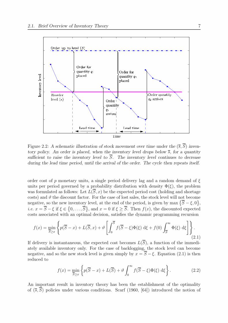
Figure 2.2: A schematic illustration of stock movement over time under the (s, S) inven-tory policy. An order is placed, when the inventory level drops below s, for a quantitysufficient to raise the inventory level to S. The inventory level continues to decreaseduring the lead time period, until the arrival of the order. The cycle then repeats itself.
order cost of p monetary units, a single period delivery lag and a random demand of ξunits per period governed by a probability distribution with density Φ(ξ), the problemwas formulated as follows: Let L(S, x) be the expected period cost (holding and shortagecosts) and ϑ the discount factor. For the case of lost sales, the stock level will not becomenegative, so the new inventory level, at the end of the period, is given by max
{
S − ξ, 0}
,
i.e. x = S − ξ if ξ ∈{
0, . . . , S}
, and x = 0 if ξ ≥ S. Then f(x), the discounted expectedcosts associated with an optimal decision, satisfies the dynamic programming recursion
f(x) = minS≥x
{
p(S − x) + L(S, x) + ϑ
[
∫ S
0
f(S − ξ)Φ(ξ) dξ + f(0)
∫ ∞
S
Φ(ξ) dξ
]}
.
(2.1)If delivery is instantaneous, the expected cost becomes L(S), a function of the immedi-ately available inventory only. For the case of backlogging, the stock level can becomenegative, and so the new stock level is given simply by x = S− ξ. Equation (2.1) is thenreduced to
f(x) = minS≥x
{
p(S − x) + L(S) + ϑ
∫ ∞
0
f(S − ξ)Φ(ξ) dξ
}
. (2.2)
An important result in inventory theory has been the establishment of the optimalityof (s, S) policies under various conditions. Scarf (1960, [64]) introduced the notion of
8 CHAPTER 2. LITERATURE REVIEW
K–convexity, a condition he used to prove the optimality of an (s, S) policy in the caseof both fixed and variable ordering costs K. A function f(x) is said to be K–convex ifthe secant line connecting any two points on the graph of the function, when extendedto the right, is never more than K units above the function, or in algebraic terms, if
f(x) + a
[
f(x)− f(x− b)
b
]
≤ f(x + a) + K, (2.3)
for a, b > 0 and all x.
Scarf [64] defined fn(x) to be the cost function associated with optimal decisions for an n–period inventory problem. He showed that the function ps+L(s)+ϑ
∫∞
0fn−1(s−ξ)Φ(ξ)dξ
is K–convex, and proved, by induction, the optimality of the (s, S) policy in the casewhere backlogging is allowed. The only constraint on the parameters of the problem isthat if the setup costs vary over time, they must decrease with increasing time.
Iglehart (1963, [31]) investigated the limiting behaviour of the value function,
fn(x) = mins≥x
{
p(s− x) + L(s) + ϑ
∫ ∞
0
fn−1(s− ξ)Φ(ξ) dξ
}
, (2.4)
and the optimal policies, (st, St), as t→∞, when the discount factor is ϑ = 1.
The nature of the demand process is an important factor that affects the type of optimalpolicy in a stochastic inventory model. The inventory control literature that followedafter 1960 is categorized according to the type of demand studied, i.e. stationary ornon–stationary, and whether the demand is fully or partially observed. In a stationarydemand process, the demand follows a single probability distribution, whilst in a non–stationary process the probability distribution of the demand varies with time. A fullyobserved process is one for which all parameters are known with certainty. A problemwith partial information is one in which the demand distribution possesses one or moreunknown parameters that may be either discrete or continuous. In the case of partialinformation, the estimate of the unknown parameters is usually updated as the actualdemand is observed over time.
2.1.1 Stationary Demand, Fully Observed
The inventory problem with fully observed and stationary demand forms the body ofmost of the classical theory of inventory control. As discussed above, Scarf (1960, [64])presented the result that if the demands during successive periods are independent andidentically distributed random variables, and the demand is fully observed, an (s, S)policy is optimal.
2.1.2 Non–stationary Demand, Fully Observed
Inventory problems with fully observed, non–stationary demand, although more complex,have also been studied extensively. The dynamic inventory model of Arrow, et al. (1951,
2.1. Brief Overview of Inventory Theory 9
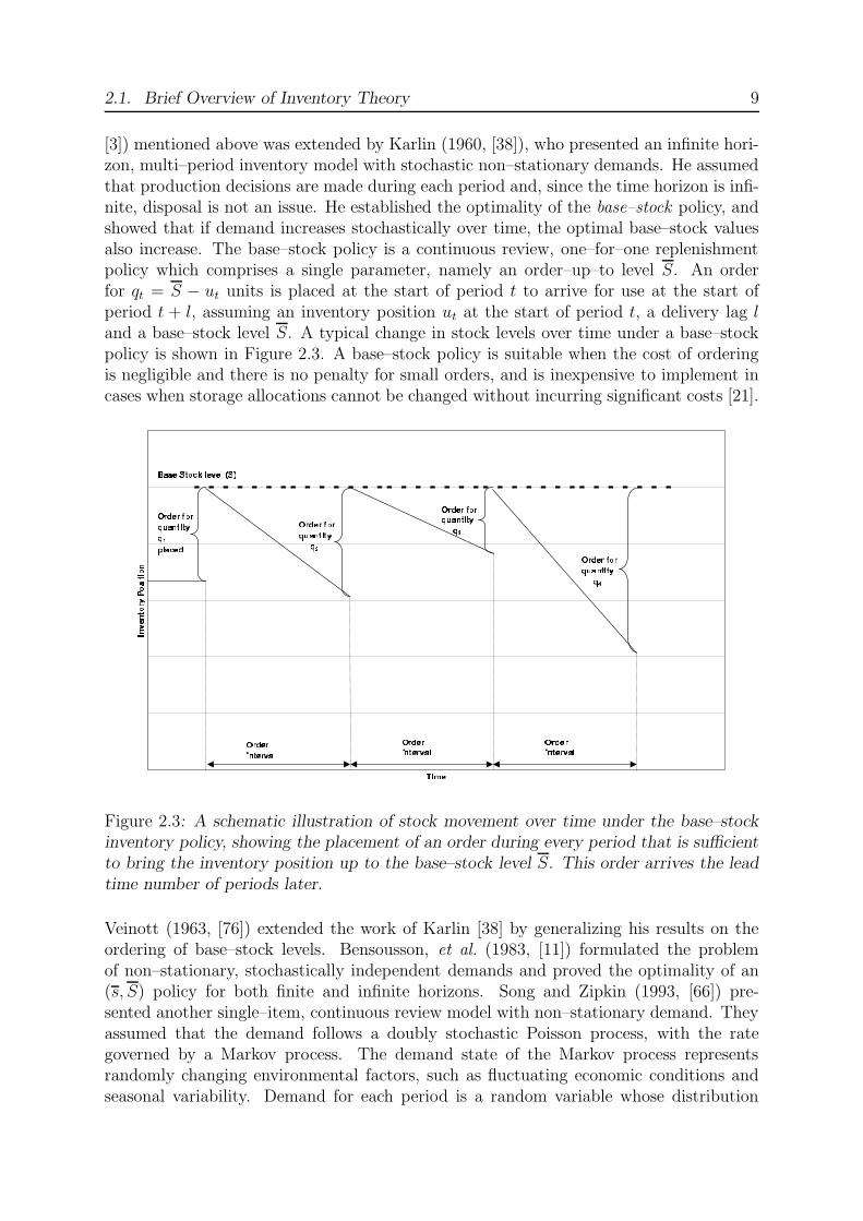
[3]) mentioned above was extended by Karlin (1960, [38]), who presented an infinite hori-zon, multi–period inventory model with stochastic non–stationary demands. He assumedthat production decisions are made during each period and, since the time horizon is infi-nite, disposal is not an issue. He established the optimality of the base–stock policy, andshowed that if demand increases stochastically over time, the optimal base–stock valuesalso increase. The base–stock policy is a continuous review, one–for–one replenishmentpolicy which comprises a single parameter, namely an order–up–to level S. An orderfor qt = S − ut units is placed at the start of period t to arrive for use at the start ofperiod t + l, assuming an inventory position ut at the start of period t, a delivery lag land a base–stock level S. A typical change in stock levels over time under a base–stockpolicy is shown in Figure 2.3. A base–stock policy is suitable when the cost of orderingis negligible and there is no penalty for small orders, and is inexpensive to implement incases when storage allocations cannot be changed without incurring significant costs [21].
Figure 2.3: A schematic illustration of stock movement over time under the base–stockinventory policy, showing the placement of an order during every period that is sufficientto bring the inventory position up to the base–stock level S. This order arrives the leadtime number of periods later.
Veinott (1963, [76]) extended the work of Karlin [38] by generalizing his results on theordering of base–stock levels. Bensousson, et al. (1983, [11]) formulated the problemof non–stationary, stochastically independent demands and proved the optimality of an(s, S) policy for both finite and infinite horizons. Song and Zipkin (1993, [66]) pre-sented another single–item, continuous review model with non–stationary demand. Theyassumed that the demand follows a doubly stochastic Poisson process, with the rategoverned by a Markov process. The demand state of the Markov process representsrandomly changing environmental factors, such as fluctuating economic conditions andseasonal variability. Demand for each period is a random variable whose distribution
10 CHAPTER 2. LITERATURE REVIEW
function is dependent on the demand state (generated by the Markov process) in thatperiod. They formulated a dynamic program to compute an optimal policy, using modified
value iteration. Modified value iteration is an algorithm for finding optimal policies forpartially observed Markov decision processes, aimed at accelerating the iteration processby reducing the number of dynamic programming updates to its convergence. Value iter-ation starts with an initial value function, which represents the expected total discountedreward for following a certain policy, and iteratively performs dynamic programming up-dates to generate a sequence of value functions, which converges to the optimal valuefunction [83]. This typically requires a large number of dynamic programming updates,so the strategy followed in modified value iteration is to improve the value functionsby means of certain additional steps. After a value function is improved by a dynamicprogramming update, it is fed to the additional steps for improvements.
Sethi and Cheng (1997, [65]) presented a more general model than that of Song and Zipkin[66], including the case of seasonal demand and incorporating service level and storageconstraints. They used the concept of K–convexity, first utilized by Scarf (1960, [64]),to establish the optimality of the state–dependent (s, S) policy in the case of Markoviandemand and full backlogging. The first assumption they made, under which the optimalpolicy is an (s, S) policy, was
Kjt ≥ K
j
t+1 ≡n∑
j=1
PjkKjt+1 ≥ 0, t ∈ T , j, k ∈ K, (2.5)
where Kjt is the fixed ordering cost for period t and demand state j, K
j
t+1 is the expectedfixed ordering cost for period t + 1 and demand state j, K = {1, 2, . . . , n} is the finite setof possible demand states, T =
{
0, 1, . . . , t}
is the planning horizon of the problem, andPjk are the transition probabilities of the Markov process, in other words the probabilityof the demand state changing from state j to state k, for all j, k ∈ K. This assumptionstates that the fixed cost of ordering during a given period with demand state j shouldbe no less than the expected fixed cost of ordering during the next period. The secondassumption made was that
pjtx + Ft+1(ft+1)(j, x)→∞ as x→∞, t ∈ T , j ∈ K, (2.6)
where pjt is the purchasing cost for period t and demand state j, x is the surplus level (of
inventory or backlog) at the beginning of a period and Ft+1(ft+1)(j, x) is the expectedholding cost. This assumption states that either pj
t > 0 or Ft+1(ft+1)(j, x) → ∞ as|x| → ∞, or both. This generalises the usual assumption that the inventory carryingcost, h, is positive. Under these and other standard assumptions, they proved that thereexist sequences of numbers sj
t , Sjt for all t ∈ T , j ∈ K, with sj
t ≤ Sjt , such that the order
quantity under an optimal policy is given by
qt(j, x) = (Sjt − x)Γ(sj
t − x), (2.7)
where the step function Γ(•) is defined as Γ(z) = 0 when z ≤ 0, and Γ(z) = 1 whenz > 0.
Graves (1999, [27]) presented a model for a single–item inventory system with a deter-ministic lead–time, but subject to a stochastic, non–stationary demand process, in which

2.1. Brief Overview of Inventory Theory 11
the demand process behaves like a random walk. The demand process is an integratedmoving average process, for which an exponential–weighted moving average provides theoptimal forecast. An adaptive base–stock policy, in which the information gained dur-ing each period is used to update the estimates of an unknown parameter (the optimalorder–up–to quantity) was proposed for inventory replenishment. It was observed thatthe safety stock required for the case of non–stationary demand is much greater than forstationary demand; furthermore, the relationship between safety stock and the replenish-ment lead–time becomes convex when the demand process is non–stationary, quite unlikethe case of stationary demand.
Kambhamettu (2000, [36]) investigated the problem of parameter estimation when theobserved demand is generated by discrete parametric probability distributions. Demandwas modelled as a partially observed Markov decision process, and it was assumed thatthe demand states are characterised by either the Poisson or the Negative Binomialdistribution. The estimation maximization algorithm, developed by Baum, et al. (1970,[9]), was applied to estimate the parameters, and the model with the best estimates wasselected.
2.1.3 Stationary Demand, Partially Observed
Stationary, partial information problems are more difficult to solve than cases where de-mand is fully observed. Scarf (1959 [63], 1960 [64]) was a pioneer in the use of Bayesiantechniques for inventory control. Bayesian analysis is a statistical procedure which en-deavours to estimate the parameters of an underlying distribution, based on the observeddata. It begins with a prior distribution, which may be based on anything, including anassessment of the relative likelihoods of parameters or the results of non–Bayesian obser-vations. In practice, it is common to assume a uniform distribution over an appropriaterange of values for the prior distribution. The Bayesian method allows for updating of thedemand distribution as new data become available, while avoiding storage of all historicaldata. It provides a rigorous framework for dynamic demand updating when the demanddistribution is not known with certainty.
Scarf (1959, [63]) studied a conventional dynamic inventory problem in which the purchasecost is strictly proportional to the quantity purchased, so that the optimal policy is definedin period t by a single critical number S, the order–up–to level. The innovation in thepaper was to allow the density of demand Φ(ξ, ω), where ξ represents the demand, todepend on an unknown statistical parameter, ω, which describes the demand density. Astime evolves, the sequence of realized demands generates holding, shortage, and purchasecosts, but in addition, more is learnt about the true value of the underlying parameter.For the analysis to be manageable, the demand distribution is assumed to take the formΦ(ξ, ω) = β(ω)e−ξωr(ξ), where β and r are functions of the unknown parameter andthe demand respectively. With this specification, if the t–th period is entered with aknowledge of the current stock level, x, and a history of past demands, ξ1, . . . , ξt−1, theentire history may be summarized in the sufficient statistic,
ν =
∑t−1i=1 ξi
t− 1, (2.8)

12 CHAPTER 2. LITERATURE REVIEW
so that the dynamic programming formulation depends only on the variables x and ν. Themonotonicity of St(ν) was demonstrated in (1959, [63]), and the asymptotic behaviour ofSt(ν) and ν, as t→∞, was determined.
Karlin (1960, [38]), Scarf (1960, [64]) and Iglehart (1964, [32]) studied dynamic inventorypolicy updating when the demand density has unknown parameters and is a memberof the exponential or range families. They showed that an adaptive critical value (ororder–up–to) policy is optimal, where the critical value is determined dynamically.
Conrad (1976, [18]) examined the effect of demand censoring by the inventory level onPoisson demand estimation. Demand censoring occurs when there are lost sales and nobackordering, resulting in partially observed demand. He proposed an unbiased maximumlikelihood estimate of the Poisson parameter.
Azoury (1985, [7]) and Miller (1986, [51]) generalised and extended the results of Kar-lin [38], Scarf [64] and Iglehart [32] to other classes of demand distributions. Azoury(1984, [6]) also investigated the effect of dynamic Bayesian demand updating on optimalorder quantities. She concluded that Bayesian demand updating, compared to the non–Bayesian method, yields a more flexible optimal policy by allowing updates of the orderquantities in future periods. The Bayesian approach is generally difficult to implement,because of extensive computational demands. Lovejoy (1990, [47]) showed that a simpleinventory policy based on a critical value (using a myopic parameter adaptive technique)may be optimal or near–optimal in some inventory models. A myopic policy is a re-plenishment policy that minimizes the average total cost per product until the inventoryis depleted, ignoring the influence of future costs on the current decision. He also gavetwo numerical examples to illustrate the performance of simple myopic policies. Lovejoy(1992, [48]) further extended this analysis of myopic policies by considering policies thatterminate the myopic behaviour at some point in time, which may be fixed or may berandom.
Lariviere and Porteus (1995, [43]) considered Bayesian techniques for a lost sales problemin which sales, not true demand, are observed. Because of lost sales, the retailer maylearn more about the true demand process by holding inventory at a higher level initiallyto establish quickly a better estimate of the true demand. Gallego, et al. (1996, [26])demonstrated a so–called Min–Max technique for the analysis of various distribution–free finite horizon models for which the distribution is specified by a limited numberof parameters, such as the mean and variance, or a set of percentiles of demand. ThisMin–Max technique is a linear programming approach, where the objective is to mini-mize the maximum expected cost over all demand distributions, satisfying a set of linearconstraints.
Ding and Puterman (1998, [20]) investigated the effect of demand censoring on the opti-mal policy in newsvendor inventory models with general parametric demand distributionsand unknown parameter values. The main result of the paper is that the combined effectof an unknown demand distribution and unobservable lost sales results in higher optimalorder quantities than in the fully observable demand case. This illustrates the trade–offbetween information and optimality, in the sense that it is optimal to set the inventorylevel higher during earlier periods in order to obtain additional information about thedemand distribution, so as to allow for better decisions during later periods.

2.1. Brief Overview of Inventory Theory 13
2.1.4 Non–stationary Demand, Partially Observed
Considerably less work has been done on the more complex inventory problems withnon–stationary demand and partial information. One paper that considers a problem inthis class is by Kurawarwala and Matsuo (1996, [42]). They presented a growth modelto estimate the parameters of a demand process over its entire life cycle. In their basecase, production decisions are made at the beginning of the problem for the entire lifecycle. They presented a technique with which the initial estimation of parameters of theirforecasting model is made. However, they do not thoroughly address the issue of revisingthese estimates, using new observations.
Treharne and Sox (2002, [73]) examined several different policies for an inventory controlproblem in which the demand process is non–stationary and partially observed. Theprobability distribution for the demand during each period is determined by the stateof a Markov chain; this underlying distribution is called the core process. However, thestate of this core process is not directly observed; only the actual demand (defined as wt)is observed by the decision maker. The inventory control problem is a composite–state,partially observed Markov decision process. For an inventory position ut, the single–period expected inventory cost function is defined as
Gt(ut|πt, l) = Ewt,l|πt[Ψ max {0, wt,l − ut}+ h max {0, ut − wt,l}] , (2.9)
where wt,l =∑l
n=0 wt+n,l represents the observed demand during the lead time l, πt isa matrix characterizing the current belief of the demand distribution, Ψ represents theunit shortage cost, h represents the unit holding cost, p represents the unit purchase cost,and Ewt,l|πt[•] denotes the expected value operator, which gives the expected value of thecost function based on the calculation of lead time demand, which is conditional on thecurrent belief of the demand distribution. The transition equation, by which the mostrecent observation, wt, is used to update πt+1, is
πk,t+1 = Tk(πt|wt = z) =
∑Nj=1 πj,trj,zPj,k∑N
j=1 πj,trj,z
, (2.10)
where rj,z is the probability that the observed demand is z, given a demand state j, andPj,k is the transition probability of the Markov decision process between states j and k.
The order quantity in period t was defined as qt, and the dynamic programming recursion
Jt(ut, πt) = −put + minyt≥ut
{
pyt + Gt(yt|πt, l) + Ewt|πt [Jt+1((yt − wt), T (πt|wt))]}
, (2.11)
where yt = ut + qt, was then shown to be convex for all ut. This demonstrates that, inthe absence of fixed ordering costs, a state–dependent base–stock policy is optimal forthe problem. In the case of a positive fixed order cost, Treharne and Sox [74] proved thatthe optimal policy is a state–dependent (s, S) policy.
Composite–state, partially observed Markov decision process problems are in practice of-ten solved by means of certainty equivalent control (CEC) policies. Under these policiessome data are observed, the unknown parameters are estimated by maximum likelihood

14 CHAPTER 2. LITERATURE REVIEW
methods, and inventory policies are chosen, assuming that the demand distribution pa-rameters equal the estimated values. However, Treharne and Sox presented results thatdemonstrate that there are other practical control policies that almost always providemuch better solutions to this problem than the CEC policies commonly used [73]. Thepolicies they compared were the myopic, limited look–ahead (LLA), open–loop feedbackcontrol (OLFC), and the CEC policies. Under the OLFC policy it is assumed that feed-back will not be used in future periods, in other words the policy does not anticipate theuse of future information about the prior distribution. It is implemented on a rolling–
horizon basis, where πt is updated using the prior observations. The LLA policy optimisesthe dynamic problem for only a limited number of periods into the future. For the myopicLLA policy, only the current period costs are minimised, in other words (2.11) is reducedto
Jt(ut, πt) = −put + minyt≥ut
{pyt + Gt(yt|πt, l)} . (2.12)
The computational results in [73] also indicate how specific problem characteristics influ-ence the performance of each of the alternative policies.
2.2 Important Concepts in Inventory Modelling
In this section, an outline is given of literature related to various concepts in inventorymodelling which are relevant to the case study presented in this thesis. One such concept,the nature of the demand process, has already been dealt with in some detail in the previ-ous section. The nature of the demand at Clickabox is non–stationary, partially observeddemand. This places it in the class of problems dealt with in §2.1.4. The transitionbetween demand states at Clickabox will be modelled as a Markov decision process. Anumber of papers concerned with Markovian–modulated demand have been mentioned in§2.1; these and other related papers will be discussed in some detail. Another distinctiveaspect of the inventory at Clickabox is its cascading product substitution. Other conceptsto be discussed in this section are lead time, stockout situations, and advance demand
information.
2.2.1 Modelling of a Markovian Decision Process
The modelling of Markovian–modulated demand was discussed in §2.1.2, in particularwith reference to the study by Sethi and Cheng (1997, [65]). The use of a Markovdecision process in the case of non–stationary, partially observed demand was introducedin §2.1.4. The methodology behind the adaptive inventory control policy proposed byTreharne and Sox (2002, [73]) and summarised in §2.1.4 will be followed in this thesis,with a number of adaptions, for the development of an inventory model for Clickabox.However, a significant adaption involves the definition of demand states. The approachtaken by Treharne and Sox [73] is that the demand states, determined by the state ofa Markov chain, represent the underlying demand distribution during that time period.Demand classes are defined, to represent ranges of values. The demand distributionsthen represent the probability of a time period demand realisation in each of the demand

2.2. Important Concepts in Inventory Modelling 15
classes. In other words, if the underlying demand distribution is weighted toward largedemand realisations (a distribution which would, for example, be in effect during peakseasons), it is probable that the time period demand realisation will be for one of thehigher demand classes. It would, however, still be possible that the demand realisationfalls into one of the lower demand classes. This approach was attempted for the Clickabox
application. However, as will be discussed in Chapter 4, the nature of the demandsuggested a modification. The demand states and demand classes are merged in thisthesis, to form just one set of demand classes, each representing a range of potentialdemand realisations. The transition between demand classes is determined by the stateof the Markov chain, and the actual demand realisation within the class is modelled bya set of probability distributions, one for each demand class.
2.2.2 Multiple Products and Stock Substitution
Veinott (1965, [77]) presented the earliest work on an optimal policy for a multi–productinventory model. This study was generalised by Ignall and Veinott (1969, [33]). Theygave conditions under which the optimal order quantity is a monotone function of theinitial inventory. Bassok, et al. (1999, [8]) followed the approach of Veinott [77] and Ignalland Veinott [33], and developed a single period, periodic review model with stochasticdemand and downward substitution. They considered N products and N demand classeswith full downward substitution, where excess demand for class i can be substituted, usingproduct j, for i ≥ j. They showed that a greedy allocation policy, for the allocation ofproducts to demand classes, is optimal. The algorithm works sequentially from product1 to product N . Demand for class i is satisfied first with stock of product i, and then ifnecessary, leftover stock of product i− 1, i− 2, . . . , 1 is used to satisfy remaining unmetdemand of class i. A similar approach is taken in the inventory model for Clickabox.However, the situation at Clickabox is more complex in the sense that strict downwardsubstitution is not appropriate. This is a result of the directional property of cardboardused in the manufacturing of boxes — each board has two properties, namely lengthand width, both of which affect the board’s structural suitability as a substitute, as asubstitute board must have both dimensions at least as large as the board for which it isa substitute. The length and width of the board are independent of each other, in otherwords if board A has a length greater than that of board B, it will not necessarily havea width greater than that of board B. Boards cannot, therefore, be arranged in a simplelist where product i is smaller than, and therefore can be substituted by, product i + 1.
Drezner, et al. (1995, [23]) considered the substitution problem for a two–product inven-tory, and established optimal order and substitution quantities, using the standard EOQmodelling approach. Drezner, et al. (2000, [22]) formulated the problem for an n–productinventory, where product j can substitute products j + 1, . . . , n, at certain costs. Theyused the same approach as Drezner, et al. [23], but found that the total cost functionmay not be convex if the number of products exceeds two. They then reformulated theproblem to determine analytically the optimal run–out time for the n products. Theyformed a new cost function, which was shown to be convex, and found the optimal deci-sion parameters (order and substitution quantities) by backward substitution. However,in both [23] and [22], demand was assumed to be known and deterministic.

16 CHAPTER 2. LITERATURE REVIEW
Downs, et al. (2001, [21]) developed a base–stock inventory model which incorporates mul-tiple products, multiple resource constraints, lost sales and delivery lags. Nonparametricestimates of the expected holding and shortage costs were developed, and a mathematicalprogramming approach was taken in determining a near–optimal policy, which comparedfavourably with the optimal solution in some numerical experiments. However, a criticalassumption of the model developed is that the cost of placing orders is negligible, whichis not appropriate in the case of Clickabox, as there is a minimum order quantity whichresults in a high penalty cost if orders for small quantities are placed frequently.
2.2.3 Stockout Situations
There are two general situations for the demand process in a stockout period — eitherthe demand is backordered, in other words customers are prepared to wait until theirdemand is satisfied, or sales are lost, in other words customers are not prepared towait, and consequently go elsewhere to satisfy their needs. The former is more widelycovered in the literature, partly because inventory studies have historic roots in militaryapplications, where the assumption of backlogging is realistic [15]. Montgomery, et al.
(1973, [53]) investigated a more realistic case — a mixture of lost sales and backorders.They considered first a deterministic demand model, and then a model with stochasticdemand for a particular case with a time–independent backorder cost and neglecting thestockout period in computing the expected order cycle length. Kim and Park (1985, [40])extended their work to allow for time–weighted backorders. This is implemented in a(Q, r) inventory model, where a fraction β of demand is backordered during a stockoutperiod, and the remaining fraction of 1− β is lost. The (Q, r) policy states that an orderof a fixed quantity Q should be placed when the inventory level drops to the re–orderpoint r. This policy is illustrated in Figure 2.4.
The (Q, r) policy is applicable to situations in which demand can only be for a single unitat a time, as the danger exists that a demand for more than one unit could reduce theinventory level to below the re–order point r, in which case the computations that led tothe calculation of the optimal re–order quantity Q are invalidated. On the other hand, the(s, S) inventory model is typically used for situations in which demand for more than oneunit at a time occurs. The model in [40] was developed, based on a heuristic treatmentof a lot–size re–order–point policy. The situation at Clickabox is in essence different tothe two general situations of backordering or lost sales, and to those in [40] and [53], inthe sense that product substitution takes place. If the optimal board to satisfy an orderis not available, the next best board is substituted, at a higher cost to the customer.The ‘lost sale’ of the optimal board is penalised in the wastage cost incurred when boardsubstitution takes place. In the case of no board being available to satisfy an order, itwill be assumed that demand is backordered.
2.2.4 Variability of Lead Time
The majority of inventory literature assumes lead time to be a constant. Bookbinderand Cakanyildirim (1999, [12]) considered a (Q, r) model with constant demand, random

2.2. Important Concepts in Inventory Modelling 17
� � �� �� �� �� � ���
� ��
�� ��������� ��� ��� ��� "!
# $$$$$$$$$$$$$$%$$$$$$$$$$$$$$&
' �(�) ��*�+-,/."0 021�435!
# $$$$$$$$$$$$$$%$$$$$$$$$$$$$$&
' ���� ��*"+-,/.�0 061�738!
# $$$$$$$$$$$$$$%$$$$$$$$$$$$$$&
' �(�� ��*"+9,/."0 021 �435!
:; , � 0 �< :; , � 0 ��
Figure 2.4: Schematic illustration of the stock movement over time under the (Q, r)inventory policy. An order for Q units is placed, to arrive the lead time number ofperiods later, each time the inventory level reaches a level of r.
lead time, and expedited orders. For expedited orders, a shorter–than–average lead timemay be obtained at a cost. The expediting factor τ is the constant of proportionalitybetween the expedited lead time and the ordinary lead time. The expected cost functionwas shown to be jointly convex in the decision variables Q, r and τ . The dynamics of leadtime variability could be incorporated into an inventory model for Clickabox. However,due to the already complex nature of the problem considered in this thesis, it will beassumed that lead time is constant, as is standard practice.
2.2.5 Advance Demand Information
Karaesmen, et al. (2002, [37]) investigated the value of advance demand information inimproving the performance of inventory systems. They discussed two cases with differingdelivery requirements. Firstly, a model was considered in which each customer announcesa future date for delivery and requires a timely delivery (i.e., the delivery may not be earlyor late). The second model assumes that the customer submits requirements in advance,and accepts early deliveries. Karaesmen, et al. [37] identified conditions in each caseunder which advance demand information may bring significant benefits. One importantfactor was found to be the average system load — the relative benefits of advance demandinformation disappear in extremely high system loads. Another factor is the nature of thedelivery requirements — if customers order in advance and accept early deliveries, thereis a significant benefit to the manufacturer. However, if early deliveries are not accepted,the value of advance demand information is not as significant. This is a topic for potentialfurther study at Clickabox, in the sense that if the value of advance demand information

18 CHAPTER 2. LITERATURE REVIEW
can be determined, rewards may be offered to regular customers for submitting orders inadvance, or in a more regular fashion. This topic, however, falls outside the scope of thisthesis.
2.3 Chapter Summary
A brief overview of literature concerning inventory theory was given in this chapter. Theinventory control literature considered was broadly divided into categories according tothe nature of the demand process, and work done in each of these categories was discussed.A number of concepts in inventory theory considered especially relevant to this study werethen explored, and their applications in the inventory model to be developed in this thesiswere discussed. The non–stationary nature of the demand process at Clickabox suggeststhe use of a Markovian decision process for the modelling of the demand, following theapproach in a number of works cited in §2.2.1. A core characteristic of the situationat Clickabox is the existence of multiple products and cascading stock substitution —various approaches to similar situations were discussed. The issue of the reaction tostockout situations was raised, as well as that of the variability of lead time. Finally,the value of advance demand information was discussed, and highlighted as an area ofpotential further study at Clickabox.

Chapter 3
Clickabox Factory
In order to develop an appropriate inventory model for Clickabox factory, it is necessaryto have a clear understanding of Clickabox ’s products, business objectives, as well asadministrative and production processes. The objective of this chapter is to providethe reader with the information necessary to gain this understanding. It is against thebackground provided in this chapter that the assumptions made for the development ofthe inventory model in Chapter 5 should be understood.
Figure 3.1: View of Clickabox from Parin Street. The office block and parking lot arevisible. To the left of the (white) office block the receiving goods entrance is visible,whilst the finished goods exit is just off the photograph, to the right.
19

20 CHAPTER 3. CLICKABOX FACTORY
3.1 Clickabox : The Business
In this section, the business objectives and business strategy of Clickabox will be dis-cussed. These are drivers of the company’s operational strategy, of which the manage-ment of its inventory forms a major part. The financial situation of the company willalso be discussed briefly, in order to give an indication of the growth in business that istaking place.
3.1.1 Business Objectives
There were two primary business objectives set out by the management of Clickabox forthe 2003 financial year. The first was to achieve a growth in real (after–tax) income ofat least 10% per annum. There were various deliverables associated with this objective,which included:
1. Achieving ISO9000 accreditation by June 2003, by measuring waste more accu-rately, reducing waste by 25%, and improving customer loyalty. The ISO9000 ac-creditation was achieved in May 2003.
2. Achieving a growth of at least 10% in annual turnover in real terms. A growth of32% was achieved over the 2003 financial year.
3. Optimising the stockholding process, by developing an inventory model, which isthe topic of this thesis.
4. The addition of die–cut capability by June 2003. This would have involved thepurchasing of a new machine, which allows boxes to be made to interlock, insteadof using the current methods of glueing or stitching. There were three optionsavailable: a roller bed die–cutter which costs approximately R100 000, a platten–type die–cutter which ranges in price from R200 000 to R1 000 000, or a rotary die–cutter, the high speed machine used by large scale manufacturers such as Nampak
[56], which costs approximately R3 000 000. The decision as to which of thesemachines to purchase has been put on hold temporarily, due to uncertain marketconditions and the resultant risk of over–capitalisation.
The second primary objective was to be a recognised leader in e–commerce in the pack-aging industry in South Africa by December 2004. It was envisaged that this objectivewould be met by achieving the following goals:
1. The development of the online quote program by June 2003 to the point whereit is a saleable product on the international market. The internet quote programexpansion was still in progress at the time of writing of this thesis.
2. Selling at least one copy of the online quote program in the financial year endingFebruary 2004.

3.1. Clickabox: The Business 21
PSfrag replacements
Turn
over
[in
104
R]
Date
0
10
20
30
40
50
60
70
80
90M
ay–88
Nov–88
May–89
Nov–89
May–90
Nov–90
May–91
Nov–91
May–92
Nov–92
May–93
Nov–93
May–94
Nov–94
May–95
Nov–95
May–96
Nov–96
May–97
Nov–97
May–98
Nov–98
May–99
Nov–99
May–00
Nov–00
May–01
Nov–01
May–02
Nov–02
Figure 3.2: The monthly turnover of Clickabox since its foundation in May 1988, with amoving average line to show the growth in turnover over the 14 year period. The periodduring which the company has been under the current ownership is indicated by an arrowon the graph.
The director of Clickabox is in the process of drawing up a business plan for this projectin conjunction with Mr Leon Swanepoel (a software developer) [69]. The plan involvesthe extension of the program to apply to not only the cardboard box industry, but alsoto other industries where two dimensional stock selection is required.
3.1.2 Business Strategy
The business strategy of Clickabox involves improving productivity through improvedmanagement and control systems. Consultants were employed to assist in the imple-mentation of ISO9000 standards during the period May 2001 to May 2003. Additionalfuture marketing and advertising channels include the company website, commission–based agents, advertising material, such as calendars and flyers, and targeted fax oremail advertisements to companies that are similar to existing customers. This thesisforms a part of the stockholding optimization project which is an integral part of the
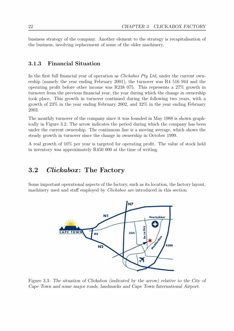
22 CHAPTER 3. CLICKABOX FACTORY
business strategy of the company. Another element to the strategy is recapitalisation ofthe business, involving replacement of some of the older machinery.
3.1.3 Financial Situation
In the first full financial year of operation as Clickabox Pty Ltd, under the current own-ership (namely the year ending February 2001), the turnover was R4 516 944 and theoperating profit before other income was R238 075. This represents a 27% growth inturnover from the previous financial year, the year during which the change in ownershiptook place. This growth in turnover continued during the following two years, with agrowth of 23% in the year ending February 2002, and 32% in the year ending February2003.
The monthly turnover of the company since it was founded in May 1988 is shown graph-ically in Figure 3.2. The arrow indicates the period during which the company has beenunder the current ownership. The continuous line is a moving average, which shows thesteady growth in turnover since the change in ownership in October 1999.
A real growth of 10% per year is targeted for operating profit. The value of stock heldin inventory was approximately R450 000 at the time of writing.
3.2 Clickabox : The Factory
Some important operational aspects of the factory, such as its location, the factory layout,machinery used and staff employed by Clickabox are introduced in this section.
Figure 3.3: The situation of Clickabox (indicated by the arrow) relative to the City ofCape Town and some major roads, landmarks and Cape Town International Airport.

3.2. Clickabox: The Factory 23
3.2.1 Factory Location and Layout
The factory is located in Parow Industrial Area (12 Parin Street), about 50km from thecity of Cape Town and 15km from Cape Town International Airport (as shown in Figure3.3).
The factory is divided into five functional areas. A floor plan of the factory is shown inFigure 3.4. The raw materials store is a 59.3m by 15m area, with access to Parin Streetfor the receiving of raw material deliveries from suppliers. Raw materials are stored indemarcated bays, which run down the length of the raw materials store, on either sideof a walkway down the centre, as shown in Figure 3.5(a). Boards may be stacked to aheight of 3.2m in these demarcated bays.
� �� �
Parking Area
15.00m
Raw Material
Store
Alley
Workshop
Finished Goods Store
Office
Waste Recovery
Area
15.00m 23
.00m
15.00m
15.00m
59.3
0m
49.7
0m
35.9
0m
Road
Figure 3.4: A floor plan of the factory, showing its division into five functional areas.
Adjacent to the raw materials store is the workshop, a 49.7m by 15m area where man-ufacturing of the boxes takes place, as shown in Figure 3.6. The equipment used in theproduction of the boxes is arranged in two production lines in the workshop, one linesuitable for large batches and the other for small batches, as the setup time and unitproduction times differ for the various machines on the two lines.
The finished goods store, shown in Figure 3.5(b), is a 35.9m by 15m area, adjacent to theworkshop and the waste recovery area. Completed boxes are stored on wooden palletsin this area, awaiting dispatch, as shown in Figure 3.5(b). It holds three categories offinished goods. The first category consists of boards that have been processed (cut down

24 CHAPTER 3. CLICKABOX FACTORY
(a) Raw Materials Store (b) Finished Goods Store
(c) Waste Recovery Area (d) Foyer to Office Area
Figure 3.5: The storerooms: The raw materials store, where the stock boards are keptin bays, the finished goods store, where goods ready for delivery are kept, and the wasterecovery area, where offcuts are kept for re–use or recycling. Also shown is the foyer ofthe office block, where administration, receiving of quotes, etc. takes place.
to creased sheets of specified dimensions, which may be folded into boxes) and packed tofill an order. These boards are generally dispatched as soon as the manufacturing of theentire order is complete. The second category consists of boards that do not require anyprocessing which are sold as is. The third category are boards that are bought specificallyfor manufacturing of a particular, popular box, for customers who regularly order boxesof the same type and dimensions. These boards are kept in the receiving area untilprocessing. They are processed as soon as there is spare capacity, and then transferredimmediately to the finished goods store. The finished goods store has access to ParinStreet for the dispatching of orders.
The waste recovery area, shown in Figure 3.5(c), is a 23m by 15m area which providesstorage space for large offcuts, which are stored for later use, and unusable offcuts, whichare recycled. Offcuts of more than 50cm in each direction are classified as re–usable.These are entered into the database as raw materials (available for use in production)

3.2. Clickabox: The Factory 25
Figure 3.6: The production area, where the manufacturing of boxes takes place. Themachinery is organised in two production lines, on either side of the central aisle. Theproduction line on the left of the photo is used for small order batches and the line onthe right is used for large order batches.
at half their original cost price. This ensures that they will be the first choice for theproduction of boxes when they are of a suitable size. Offcuts of more than 50cm in justone direction are entered into the database as raw materials, but at a price of zero, and sowill also be used as soon as possible. Other offcuts are put into a bin for recycling. Thesescraps are collected weekly by Nampak [56], who pays Clickabox R0.38/kg for the scraps.This results in an income of approximately R750 per month. The entire waste recoveryoperation, including both the recycling and re–using of offcuts, currently generates anincome of approximately R1 875 per month [75].
Finally, there is an office area at the front of the warehouse, approximately 5m by 15m indimension, where the administration, receiving of quotes, etc. takes place. This comprisesa separate office for the director, a meeting room, and adjacent offices for the otheradministrative staff. This gives a total floor area of approximately 2518.5m2. The foyerat the entrance to the office area is shown in Figure 3.5(d).

26 CHAPTER 3. CLICKABOX FACTORY
(a) Slitter/Creaser (b) Beamslotter
(c) Stapler (d) Strapper
Figure 3.7: Machinery used for small order batches, and the strapper. The Slitter/Creasercuts the cardboards into sheets, and makes the required creases. The Beamslotter cutsslots in the boards for folding. The Stapler uses metal staples to join box flaps, and thestrapper bundles the completed boxes together.
3.2.2 Workshop Machinery and Manufacturing Process
As mentioned in §3.2.1, the equipment used for the production of cardboard boxes is ar-ranged in two production lines in the workshop, one line suitable for large order batchesand the other for small order batches. Machines are set up manually according to specifi-cations on a so–called works ticket, which is printed for each order. All machines requirethe operators to feed through the cardboard manually. Boxes are manufactured accordingto a cutting pattern, which specifies the required creases and slots that need to be cutinto the cardboard.
Small order batches are processed by three machines in succession. These machines areshown in Figure 3.7(a)–(c). The first machine in this sequence is the slitter/creaser(Figure 3.7(a)), which cuts the cardboards into sheets of the required dimensions, andmakes creases in the cardboard as required for folding. This machine has an average setup

3.2. Clickabox: The Factory 27
(a) Printer/Slitter/Creaser (b) Gluer
Figure 3.8: Machinery used for large order batches. The Printer/Slitter/Creaser cutsboards into sheets, makes the required creases, and prints in one or two colours. TheGluer joins the folds of boxes.
time of 3 to 10 minutes, depending on the number of creases required, and a productionrun time of approximately 400 sheets an hour, for average sheet sizes [24].
The second machine is the beamslotter (Figure 3.7(b)), which cuts slots into the card-board, as specified on the works ticket. The beamslotter has a setup time of 5 minutes,and a production run time of approximately 205 sheets an hour [24].
Finally, there are four staplers, which are used to join the box flaps (one is shown inFigure 3.7(c)). The customer may choose whether to have the boxes stapled or glued,but in general, when it is not specified, the stapler will be used for the small order batches.
There are also two strapping machines (one is shown in Figure 3.7(d)), which are usedto bundle the completed boxes together, so that bundles may be transported togetherconveniently and tidily.
Larger order batches are processed by the printer/creaser/slotter (shown in Figure 3.8(a))— a single machine which performs all the functions of the slitter/creaser and the beam-slotter, as well as any printing on boxes, if required by the customer. This machine takeslonger to set up than the other machines, 35 to 200 minutes, depending on the numberof colours to be printed, but it is more efficient for large batch processing, as it has ashorter unit processing time (approximately 800 sheets per hour) [24].
The boxes in large order batches are then joined by the carton glueing machine, shownin Figure 3.8(b). The gluer has a 15 minute setup time and a processing time of approx-imately 800 sheets per hour [24].
There are two forklifts used to transport the boards around the factory (see Figure 3.9(a)).Completed boxes are delivered to the customer using the delivery vehicle shown in Figure3.9(b).

28 CHAPTER 3. CLICKABOX FACTORY
(a) Forklift (b) Delivery Vehicle
Figure 3.9: A forklift is used for moving piles of boards or boxes around the factory, anda delivery vehicle is used for transportation of the finished goods to the customer.
The stages of the manufacturing process described here are illustrated schematically inFigure 3.10.
3.2.3 Factory Staff
Piet and Miemie Taljaard are the owners and directors of the company, and it is man-aged by Piet Taljaard. There are eight other permanent staff members: a supervisor ofquotes and technical issues, an accountant, and six factory staff members, who performproduction tasks in the workshop. When necessary, in periods of high demand, additionalworkers are employed (generally up to three) on an hourly basis [70].
3.3 Raw Materials
Most raw materials are ordered from Mondi [52]. Other suppliers, such as Nampak [56],are used when Mondi cannot meet the demand. Figure 3.11 shows a raw materialsdelivery being received at Clickabox.
Cardboard is classified by its type, flute and category. There is a range of cardboardtypes available from Mondi. Of these, only two types are kept in stock at Clickabox.These are the Mondi Liner (single corrugated board) and Double Wall Board (doublecorrugated board). The reason for this is that the other types are more expensive andtherefore less popular. If required, these boards may be bought in for special orders. The

3.3. Raw Materials 29
Raw Material Arrival
Sell as is or process further?
Finished Goods Store
Sell as is
Raw Material
Store
Process further
Order Received
Large or small batch?
Slitter\Creaser
Beam Slotter
Stapler Printer\Creaser\Slotter
Gluer
Large batch
Small batch
Finished Goods Store
Figure 3.10: Manufacturing Process Flow Diagram
single corrugated board is the most common material used. Double corrugated board isused when stronger boxes and extra padding are required. Cross sections of these twocardboard types are shown schematically in Figure 3.12.
The flute type describes the structure of the wave shaped cardboard material that makesup a board’s corrugation. There are a number of flute types, each with a differentthickness and therefore different usages. The flute types used by customers of Clickabox
are described in Table 3.1. Double corrugated board is composed of a combination of a Band a C flute. The fluting gives the board a directional property, the width of the board ismeasured in the flute direction. The directional property is important in the productionprocess as it determines to a large degree the structural properties and strength of a box.
Cardboards are divided into categories, dependent on their quality and thickness. Inthe industry, these are referred to as classes, however the term classes will be used in adifferent sense in this thesis. Hence classes of cardboard will be referred to as categories.The categories allow for a balance between cost and performance for various applications.Thickness of linerboard increases from Category A (typically 140 or 150g/m) to Category

30 CHAPTER 3. CLICKABOX FACTORY
Figure 3.11: A truck bringing a delivery of raw materials from a supplier to the deliveryentrance of Clickabox, in Parin Street.
(a) Profile of a Single Corrugated Board (b) Profile of a Double Corrugated Board
Figure 3.12: Profiles of the two cardboard types kept in inventory at Clickabox.
D (typically 250g/m). The fluting is likely to deform the liner of Category A board,making the back of the board unsuitable for printing or lamination. However the thickerCategory C and D boards may be laminated on both sides.
3.4 Order Classification
There are three classes of orders received by Clickabox, namely:
Standard Orders: These comprise orders for box types, such as “A4”, which can only bemanufactured in one way, or recurring orders for an established customer, such asContinental China [17], which has a few set box orders. The raw materials used forthese standard orders may therefore be processed as soon as they arrive and thereis spare time in between the production of other orders, as mentioned in §3.2.1, andneed not be kept (unprocessed) in the warehouse. The processed material is thenstored as “Finished Goods Stock”. This produce will always be either on hand oron order, as it is re–ordered as soon as levels are low. Some raw materials are sold

3.4. Order Classification 31
FLUTE THICKNESS COMMENTS
C 4.4 mm good stacking strengthgood crushing resistancevery common materialtypical packaging for glass, furniture, dairy products
B 3.2 mm good puncture resistanceless space consumed in warehousetypical packaging for canned goods, displays
E 1.6 mm light weightstrong alternative to paper boardsuperior printing surfaceexcellent for custom die cut boxestypical packaging for displays, point of purchase boxes
Table 3.1: The properties and usages of the different flute types available.
as is. Boards currently used for standard orders, at the time of writing, are shownin Table 3.2.
Reference Type Category Flute Size (in mm)Stock 600 Mondi Liner A C 600×400×400Stock 505 Mondi Liner A C 505×350×355Ref A3 Mondi Liner B C 430×305×290Ref A4 Mondi Liner B C 305×215×290P–AD4 Mondi Liner B C 440×360×408P–EXP Double Wall Board A B and C 526×418×318P–ONT Double Wall Board A B and C 458×458×254P–W2 Mondi Liner B C 500×250×250P 1 Mondi Liner B C 560×334×500P 3 Mondi Liner B C 560×334×286P 4 Mondi Liner B C 750×463×200PTD Mondi Liner B C 750×463×140PTS Mondi Liner B C 750×463×70
Table 3.2: The properties of the standard order raw materials boards (in other words,boards used for boxes commonly ordered from Clickabox), which may be manufactured assoon as the raw materials arrive, when there are spare time lulls in between the productionof other orders.
Special Orders: These are orders for boxes not commonly ordered, such as for boxes ofa flute type not stocked by Clickabox. The cardboard required to produce theseorders is therefore brought in on request and not kept in inventory.
Standard Stock Orders: These are orders that utilise the board sizes most commonlyordered, as determined from experience. These are the board sizes kept in inventory,and used by Clickabox ’s quote program in the preparation of a quote and orderform. A section of this thesis will be devoted to determining the ideal dimensionsof standard stock board to be kept in inventory, in order to minimize expectedaverage wastage. Prior to this study the standard stock profile consisted of 28

32 CHAPTER 3. CLICKABOX FACTORY
different sizes of Category A, Flute C board (termed AC board) and 18 sizes ofDouble Wall Board (termed DWB board). The make–up of the previous stockprofile is given in Table 3.3.
Category Flute Length Width(in mm) (in mm)
A C 1 000 1 400A C 1 220 21 00A C 1 250 1 300A C 1 360 2 100A C 1 400 1 300A C 1 425 1 125A C 1 500 1 500A C 1 530 1 300A C 1 540 910A C 1 550 1 400A C 1 555 1 540A C 1 600 1 300A C 1 650 1 500A C 1 700 1 000A C 1 700 1 200A C 1 710 1 500A C 1 850 1 510A C 1 860 1 200A C 1 870 1 055A C 1 920 910A C 2 000 1 200A C 2 000 1 500A C 2 100 1 000A C 2 200 1 200A C 2 200 1 500A C 2 300 1 000A C 2 300 1 200A C 2 358 1 062
(a) Dimensions of AC Stock Board
Category Flute Length Width(in mm) (in mm)
DWB DWB 1 200 2 100DWB DWB 1 350 2 100DWB DWB 1 350 2 270DWB DWB 1 440 1 020DWB DWB 1 500 1 050DWB DWB 1 500 1 300DWB DWB 1 500 1 400DWB DWB 1 600 1 000DWB DWB 1 600 1 800DWB DWB 1 700 1 200DWB DWB 1 840 1 200DWB DWB 1 850 1 500DWB DWB 1 920 1 800DWB DWB 2 000 1 200DWB DWB 2 120 1 510DWB DWB 2 200 1 350DWB DWB 2 300 1 600DWB DWB 2 380 1 200
(b) Dimensions of DWB Stock Board
Table 3.3: Standard stock, the board sizes kept in inventory at Clickabox prior to thiscase study, from which boxes ordered as ‘quick orders’ were manufactured.
3.5 Processes at Clickabox
The current inventory control processes of Clickabox are described in this section. Thiswill allow for a meaningful evaluation of the results obtained by the inventory modeldeveloped in Chapter 5, in terms of feasibility of the model, the costs of implementingthe model, and potential savings as a result of the model solution (in Chapter 6). Theprocesses followed by Clickabox, from providing quotations to the delivery of finishedboxes, are then described.

3.5. Processes at Clickabox 33
3.5.1 Ordering of Stock from Raw Materials Suppliers
The minimum order quantity per raw material board size that Clickabox may order fromits suppliers for each order is 1 000 units. However, orders of 500 boards are takensubject to a surplus cost of R0.37 per board. Furthermore, Mondi [52] specifies that,where possible, orders should be deckled to one of two widths in order to fit the width oftheir machinery. Orders are processed at the supplier as soon as the deckle width is full.For punctual delivery, it is optimal to place an order which fills the deckle width. So if,for example, one orders a type B flute, which is uncommon, one must either wait for avery long time or pay for the full width of the cardboard from which boards are cut. Thedeckle widths are 2 415mm and 2 275mm.
The minimum order quantity policy was, however, under review at the time of writing,and furthermore, it is possible for Clickabox to use other suppliers who do not imposeminimum order quantities. These restrictions will therefore not be included in the modelwhen computing the suggested raw material re–order quantities. The concept of minimumorder quantities is, instead, cited as a potential area of future study at Clickabox.
Currently, a continuous review (s,S) inventory policy is followed at Clickabox. Re–ordering is done daily, when necessary. Two values are defined for this policy:
Re–order level, s: The stock level at which re–ordering of stock should take place.
Order–up–to level, S: The stock level up to which the replenishment order brings thestock on hand.
Each morning the stock level of each board type used the previous day is taken. If thelevel has fallen below the re–order level, an order is placed for the re–order quantity.Currently the re–order level is 300 for all board types. The order–up–to–level is 800 forDWB boards and 1300 for AC boards. The lead time for orders to arrive is approximatelytwo weeks.
3.5.2 Ordering of Boxes from Clickabox by clients
The processes followed by Clickabox when receiving orders from customers during thegeneration of a quotation, and during the manufacturing of boxes, are described in thissection.
Box dimensions and types
In the packaging industry, the size of corrugated boxes is expressed by three dimensions:Length (L), Width (W ) and Depth (D), all in millimeters (mm). These measurementsrefer to the inside dimensions of the box. The length, L, is the larger dimension of theopening, the width, W , is the smaller dimension of the opening and the depth, D, isthe dimension perpendicular to the opening. This differs from the terminology used for

34 CHAPTER 3. CLICKABOX FACTORY
L W
L W
D D
W/2
W
W/2
L
Figure 3.13: The ‘Regular Slotted Carton’, and the cutting pattern according to whichit is manufactured.
L L W/2
D
W
W/2 W/2 W/2
W
L
D W
Figure 3.14: The ‘Tuck–in–Flap’ box, and the cutting pattern according to which it ismanufactured.
cardboard sheets, where the length and width are determined by the directional propertyof the fluting, as discussed previously.
There are a number of different box styles that may be ordered by clients, each withdifferent creasing and cutting requirements. The most commonly ordered box style is the‘Regular Slotted Carton’. This box is produced from one sheet of cardboard, with verylittle manufacturing wastage and is therefore the most economical. The Regular SlottedCarton is shown schematically, together with its cutting pattern, in Figure 3.13.
Another box style, the ‘Tuck–in–flap’, is shown together with its cutting pattern in Figure3.14.
Quote Generation
The Clickabox website [57], mentioned in §1.1.2 and from which Clickabox derives itsname, provides customers with access to a computer program which allows the user to
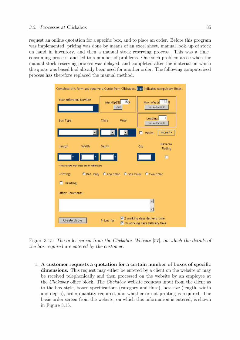
3.5. Processes at Clickabox 35
request an online quotation for a specific box, and to place an order. Before this programwas implemented, pricing was done by means of an excel sheet, manual look–up of stockon hand in inventory, and then a manual stock reserving process. This was a time–consuming process, and led to a number of problems. One such problem arose when themanual stock reserving process was delayed, and completed after the material on whichthe quote was based had already been used for another order. The following computerisedprocess has therefore replaced the manual method.
Figure 3.15: The order screen from the Clickabox Website [57], on which the details ofthe box required are entered by the customer.
1. A customer requests a quotation for a certain number of boxes of specificdimensions. This request may either be entered by a client on the website or maybe received telephonically and then processed on the website by an employee atthe Clickabox office block. The Clickabox website requests input from the client asto the box style, board specifications (category and flute), box size (length, widthand depth), order quantity required, and whether or not printing is required. Thebasic order screen from the website, on which this information is entered, is shownin Figure 3.15.

36 CHAPTER 3. CLICKABOX FACTORY
2. The required sheet (cutting pattern) dimensions are calculated. The sheetdimensions are determined by the box dimensions and style. These dimensionsinclude an allowance for creasing, which is dependent on the flute and cardboardtype. The creasing allowances are given in Table 3.4.
Type Flute Creases Wall thickness Creases Wall thicknessagainst flute in flute in flute against flutedirection (a) direction (b) direction (c) direction (d)
SC B 3 2 9 1SC C 5 3 10 3SC E 2 2 5 1
DWB B and C 9 6 18 7
Table 3.4: Creasing allowances (in mm), dependent on flute and cardboard type. Theseallowances are included in the calculation of the dimensions of the cardboard sheet re-quired to manufacture the board ordered.
For example, the dimensions of the sheet required to manufacture a Regular SlottedCarton of length L, width W , and depth D are then (L + a) + (W + a) + (L + a) +(W + d) by (W/2 + b) + (D + c) + (W/2 + b), as illustrated in Figure 3.16, wherethe symbols a, b, c and d are as defined in Table 3.4.
W/2+b
D+c
W+d
L+a W+a W+d L+a
Figure 3.16: The dimensions of the sheet required to manufacture a regular slotted cartonof length L, width W and depth D.
3. The delivery option is selected. The customer must also decide whether toorder from stock, in which case lead time for the order is two working days, or totake the “buy–in” option. This is the cheaper option for the client: exactly theright cardboard size is ordered from the suppliers for manufacturing and thereforethere is no wastage. The disadvantage is that the order may take more than sevenworking days if this option is executed.
4. A list of boards that may be used in the manufacturing of the requiredboxes is compiled. If the “buy–in” option is chosen, a board of the optimal size

3.5. Processes at Clickabox 37
is ordered from the supplier, and it is priced accordingly. If not, the program thensearches through all the boards in the Pastel database (where on hand inventorydata is stored) to obtain a list of viable boards from which the required sheet may becut. This list is sorted in order of increasing wastage, and then available quantitiesare checked. The result is an array of boards, the on hand inventory of that board,and the cost of using that board.
5. A quote is compiled. Activity based costing is used. A fixed setup cost is charged,and divided by the number of boards ordered to give a unit cost per board. This isthe only form of quantity discount given, in that the greater the quantity of boardsordered, the lower the unit allocation of the fixed cost. This is added to the variablecost (dependent on the production time for that board type) and raw materials costper board, and the full amount is multiplied by a markup. The average markup is1.45; discounts are given to larger customers.
This costing information is presented to the user in the form of an invoice. Aquotation generated for the “buy–in” option is shown in Figure 3.17, and a quotationgenerated for the same order using the stock board option is shown in Figure 3.18.The price quoted is calculated on the total area used, so the use of sub–optimalboards is more expensive.
Figure 3.17: The quotation screen from the Clickabox Website [57], giving a quotationfor a buy–in board order — one of the two options available to the customer, includingthe price and creasing information.
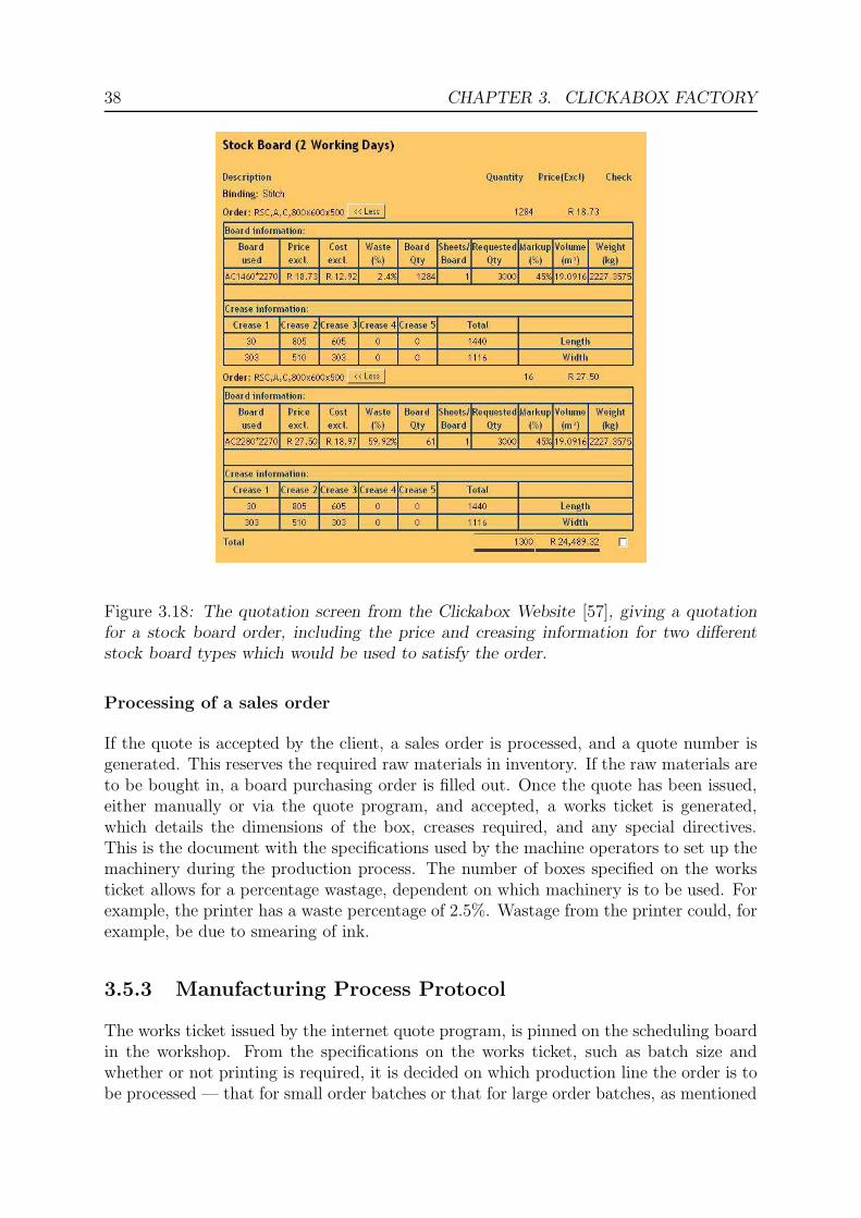
38 CHAPTER 3. CLICKABOX FACTORY
Figure 3.18: The quotation screen from the Clickabox Website [57], giving a quotationfor a stock board order, including the price and creasing information for two differentstock board types which would be used to satisfy the order.
Processing of a sales order
If the quote is accepted by the client, a sales order is processed, and a quote number isgenerated. This reserves the required raw materials in inventory. If the raw materials areto be bought in, a board purchasing order is filled out. Once the quote has been issued,either manually or via the quote program, and accepted, a works ticket is generated,which details the dimensions of the box, creases required, and any special directives.This is the document with the specifications used by the machine operators to set up themachinery during the production process. The number of boxes specified on the worksticket allows for a percentage wastage, dependent on which machinery is to be used. Forexample, the printer has a waste percentage of 2.5%. Wastage from the printer could, forexample, be due to smearing of ink.
3.5.3 Manufacturing Process Protocol
The works ticket issued by the internet quote program, is pinned on the scheduling boardin the workshop. From the specifications on the works ticket, such as batch size andwhether or not printing is required, it is decided on which production line the order is tobe processed — that for small order batches or that for large order batches, as mentioned

3.5. Processes at Clickabox 39
in §3.2.2. This decision, made by the foreman on the floor, may also be influenced by thecurrent workloads on either production line.
The boards are then cut to size, and the printing, slotting, creasing and joining areperformed, as described in §3.2.2. Once the boxes have been manufactured, it is confirmedexactly how many boards were used for the order. There are a number of possible causesfor discrepancies in this figure. The works ticket contains an allowance for wastage— if, for example, 700 boxes are ordered, it may be calculated that 714 need to bemanufactured, taking into account the waste allowance. It is possible, however, thatthere may only be raw materials to produce 710 boxes in the warehouse, as a deliveryof raw materials could have been 10 boards short. Then only 710 will be made, so thisneeds to be entered on the works ticket and the inventory updated accordingly. There aredaily stock–takes of the raw materials in order to keep inventory information as accurateas possible.
The completed boxes are finally moved to the finished goods store, where they are stackedand await dispatching. Offcuts are moved to the Wastage recovery area for re–use orrecycling.
3.5.4 Administrative Manufacturing Process
The accounting package used is Pastel Manufacturing [58]. All information about stock— raw material and finished goods, clients etc. — is stored in this system. Each rawmaterials type is assigned a code, and each box order is associated in Pastel with a setof raw material codes. This is known as the Bill of Materials. An example of a Bill ofMaterials from Pastel is shown in Figure 3.19.
CLICKABOX (PTY) LTD 27/06/2001 14:22 Page: 1Prepared by: CORRUCAPE (PTY) LTD
Bill of MaterialsCode : 505 AC/RSC/505*350*355Manufactured Item : 505 505 × 350 × 355
Item Description Unit Quantity Average Cost Last Cost505–AC 1 748 × 717 Cr 176–365–176 1.000 3.277 3.170Total for Components 3.277 3.170
Cost 1 0.000 0.000Cost 2 0.000 0.000Cost 3 0.000 0.000Total Cost for Manufactured Item 3.277 3.170Update Manuf. Selling Prices : NoNo. of Notes : 0
Figure 3.19: Bill of Materials
When a box is manufactured, it is necessary to perform a process, known as the adminis-trative manufacturing process, in order to update the inventory. A finished goods code isgenerated, representing the type and dimensions of the finished box. The finished goodsinventory is credited with the number of these boxes manufactured. The raw materialsthat made up the boxes, as specified in the Bill of Materials, are subtracted from the rawmaterials inventory.
40 CHAPTER 3. CLICKABOX FACTORY
3.5.5 Post Manufacturing Process
Once completed, the boxes are bundled and strapped together so that they are easy tohandle in batches. A delivery note is completed with the totals of boxes to be deliveredand is attached to order bundles; this is signed on delivery. An invoice is sent out toclients after delivery, and statements are sent at the end of each month.
3.6 Chapter Summary
The various processes of Clickabox factory were described in some detail in this chapter,in order to provide the reader with an understanding of the environment in which thisstudy was conducted. The business strategy and objectives of the factory were discussedin §3.1, as well as its financial situation, highlighting the importance to Clickabox ofan efficient inventory management system. The layout, products and processes of thefactory were described in §3.2–3.5, focussing, in particular, on previous inventory controlpractice.
Chapter 4
Analysis of Board Demand
There are a number of factors influencing the demand for cardboard boxes. The cor-rugated carton industry in the Western Cape is highly dependent on the fruit industry,and so demand increases notably during the fruit–picking season, May and October toJanuary. Also, being a small but growing manufacturer, the averages of board size andquantity ordered from Clickabox may be affected significantly with the acquisition of evenone new, large client [70]. Thus any calculations of optimal board or re–order strategymust be dynamic. The orders placed over a two year period for boxes from Clickabox
factory1 were analysed in order to answer the first research question formulated in §1.2(which boards to keep in stock) and to begin the process of answering the second re-search question (what inventory policy to follow) by examining the nature of the demandprocess. The demand data available are described in §4.1, and then the various stepstaken towards determining an optimal set of stock boards to be held in inventory, basedon these historic data, are described in §4.2. Finally, in §4.3, the nature of the demandprocess is discussed, and the way in which this demand will be modelled in Chapter 5is detailed. The notion of board preference vectors is introduced, and a set of demanddistributions for each of these board preference vectors is derived.
4.1 Description of Demand Data
Data from the period 1 February 2001 — 31 January 2003 were used to obtain an impres-sion of demand at Clickabox. This set of data was extracted from works tickets which arestored by Clickabox in excel worksheets for each board manufactured. It was analyzedby means of a program written by the author in Visual Basic [50]2. Data were extractedfrom a total of 3 965 works tickets, representing all orders processed during the periodmentioned above. February 2001 is the earliest period for which data were available, asit is only since then that works tickets have been created electronically and stored byClickabox.
1A snapshot of this data is given in Appendix D. The full list of works tickets is included on a CDinside the back cover of this thesis.
2The relevant Visual Basic source code, as well as the structure of the Microsoft Access databasetables, are given in Appendix C.
41

42 CHAPTER 4. ANALYSIS OF BOARD DEMAND
The following details of each order were observed:
• Order Date. The date on which the order was placed.
• Board Style. The type, category and flute of cardboard required to process theorder.
• Box Design. The design of the box required, for example a regular slotted carton.This design influences the dimensions of the board required to manufacture the box.
• Box Dimensions. The length, width and depth of the required box.
• Quantity. The number of boxes ordered.
• Sheet dimensions required. The dimensions of the sheet (length and width)required to produce the box ordered, calculated from the box dimensions, style anddesign, with standard provisions for wastage, etc. For the purposes of establishingdemand distributions in this chapter, and for the inventory model which will bedeveloped in Chapter 5, customer orders are considered to be sheet orders, i.e.
the box design and dimensions are no longer relevant, only the dimensions andcardboard type of the sheet are required.
• Board used. A list of the dimensions of the boards actually used to process eachorder, is stored. Each sheet may be produced by a number of boards, with varyingamounts of wastage associated with each board type chosen to fulfil an order for aspecific sheet type. Multiple board types may be used to process an order, if thereis not sufficient stock to process the entire order with the optimal board. The worksticket lists all board types, and the quantity of each board type that was used, inorder of preference (in terms of wastage incurred).
CLICKABOX WORKS TICKET Date: 27/02/2002Design: RSC Board Type: DWB R/m2: R4.46Size: 550 × 330 × 430 Printing: Ref onlyQuantity: 50 Delivery: 05/03/2002 Joint: StitchDelivery address: Reactor Road, Stikland Triangle FarmCreasings: 35 559 339 559 337 Sheet Length: 1829
171 448 171 Sheet Width: 790Stock Board Quantity Sheets/board % Waste Board AreaDWB 1920×0900 10 1L×1W=1 18.94% 1 728 000DWB 1920×1800 15 1L×2W=2 18.94% 3 456 000DWB 2100×1700 25 1L×2W=2 22.87% 3 570 000
Figure 4.1: Works ticket produced upon a client’s acceptance of a quotation, indicatingthe board style, box design and dimensions, delivery details, and the quantity required,as well as creasing and printing instructions. Also indicated are the stock boards fromwhich this order will be produced, and the quantities of each board that will be used.
An example of a works ticket is given in Figure 4.1.

4.2. Determining Suggested Stock Board Profile 43
4.2 Determining Suggested Stock Board Profile
The steps taken towards determining an optimal set of stock boards to be kept in inven-tory, using the historical data described in the previous section, are now described. AnABC analysis was conducted on the various cardboard types available, and the cardboardtypes responsible for the largest percentage of annual profit were determined. The resultsof this analysis are given in §4.2.1. The demand data for these cardboard types were thenanalysed, and a heuristic was used to determine a set of suitable stock boards (as detailedin §4.2.2–4.2.4) to be kept in stock. The resulting set of boards recommended to be keptin inventory is given in §4.2.5, and compared to the previous stock profile.
4.2.1 ABC Analysis of Cardboard Types
Pareto’s law is a concept developed by Vilfredo Pareto, a 19th century Italian economist,who noticed a common phenomenon that a small percentage of a group of individualstypically accounts for the largest fraction of the group impact [55]. ABC Analysis is aform of Pareto analysis, developed by General Electric during the 1950’s, and appliedto a set of products kept in inventory in order to classify them according to financialimpact [81]. The ABC Classification places items into three basic categories, which maybe treated differently in the processes of stock planning and control. These categoriesare:
Class A Items: Items that, according to an ABC classification, belong to a small setof products that represents approximately 75–80%3 of the annual demand, usageor production volume, in monetary terms, but only some 15–20% of the inventoryitems. For the purpose of stock control and planning, the greatest attention is paidto this category of products. Class A items typically are of strategic importance tothe business concerned.
Class B Items: An intermediate set of products, representing approximately only 15–20% of the annual demand, usage or production value, but some 20–25% of thetotal number of inventory items. Less management attention is paid to this classthan to the Class A items.
Class C Items: Products which, according to an ABC classification, belong to the 60–65% of inventory that typically represent only approximately 5–10% of the annualdemand, usage or production value. Least attention is paid to this category for thepurpose of stock control and planning.
The first step in an ABC Classification at Clickabox was to determine a ranking, accordingto the total profit yielded by each cardboard type per year, termed the annual usagevalue4. Profit per board was calculated as the difference between raw material cost and
3These percentages represent typical values, which will vary for different sets of data. In the classifi-cation process, only the percentage of items is set for each class, the usuage value represented by eachclass is then derived [55].
4The profit per board multiplied by the average number of boards of that type sold in a year.

44 CHAPTER 4. ANALYSIS OF BOARD DEMANDPSfrag replacements
Usa
geva
lue
%
Cardboard type
Usage value %Cumulative usage values %
AC DWB AB BC CC BB0
10
20
30
40
50
60
70
80
90
100
Figure 4.2: The individual and cumulative usage values of the six cardboard types avail-able, used for the ABC classification of the cardboard types at Clickabox.
board selling price (per square metre) multiplied by the average board size for that type.Next, products were ranked in order of decreasing usage value. The cumulative usagevalue was then calculated progressively, and expressed as a percentage of the total usagevalue. These cumulative usage values are shown in Figure 4.2.
Finally, the cumulative percentage of items was derived, by expressing the rank numberas a percentage of the total number of items (here, cardboard types). In other wordseach cardboard type comprises 16.6% of the number of different cardboard types thatmay be kept in inventory. The class break points were then set, as shown in Figure 4.3and Table 4.1, with the top 16.6% of the items (cardboard type AC) being classified asClass A items, the next 16.6% of the items (cardboard type DWB) being classified asClass B items, and the remaining 66.6% of the items (cardboard types AB, BC, CC andBB) being classified as Class C items.
The results of this analysis showed that the cardboard type “AC” is a Class A Item,accounting for approximately 59% of the profit, the “DWB” boards are Class B Items,accounting for approximately 35% of the profit, and the other cardboard types are theClass C Items, collectively accounting for approximately only 6% of the profit. It wasconsequently decided that the analysis of Clickabox’s inventory policy would focus on ACand DWB boards only.

4.2. Determining Suggested Stock Board Profile 45
Rank Cumulative Board % Usage Cumulative % Class% of Items Type Value Usage Value
1 16.6 AC 58.92 58.92 A2 33.3 DWB 34.56 93.48 B3 50.0 AB 3.07 96.55 C4 66.6 BC 1.83 98.38 C5 83.3 CC 0.93 99.31 C6 100 BB 0.69 100.00 C
Table 4.1: Determination of the class break points, in terms of the usage value, for thedifferent classes of items (cardboard types) in the ABC classification at Clickabox.
PSfrag replacements
% of Products
Cum
ula
tive
%of
Usa
geVal
ue
Class
Class
Class
“A”
“B”
“C”
Items
Items
Items
0 10 20 30 40 50 60 70 80 90 1000
10
20
30
40
50
60
70
80
90
100
Figure 4.3: Graphical representation of the class breakpoints in the ABC Classification,showing the cumulative percentage of the total usuage value represented by each class ofproducts.
4.2.2 Graphical Representation of Data
Given the results of the ABC analysis, it was decided that the demand data will beanalysed as two separate sets, namely Category A — Flute C board (AC cardboardtypes) and Double Wall Board (DWB cardboard types). Other grades of board may bebought in for special orders and should not be kept in stock, as cumulatively they account

46 CHAPTER 4. ANALYSIS OF BOARD DEMAND
for less than 7% of the annual usage value.
The scatter charts in Figure 4.4 were plotted to give a graphical indication of the distri-bution of order sizes for sheets of various dimensions of both AC and DWB cardboardtypes. They show the considerable range of different sheet dimensions ordered, one of theproperties of the demand profile of Clickabox that makes both the choice of stock boardsand the choice of inventory control policy difficult.
� � � � ��� � � ��� � � � � � � � � � ��
� ���
��� � �
��� � �
� � ���
� � ���
� ���
�� �����
��������������
���������
��� �������! �"�#�$ % $ &
(a) AC Board
' ( ' ' )�' ' ' )�( ' ' *+' ' ' *+( ' ''
( ' '
)�' ' '
)�( ' '
*+' ' '
*+( ' '
, -./01
243 5+6 7
8!9�9�9
:�9�9�9
;�9�9�9
(b) DWB Board
Figure 4.4: Scatter charts representing all orders placed over the two year period 1February 2001 — 31 January 2003, for each of the class A and B cardboard types, givingan indication of the range of sheet dimensions ordered from Clickabox, and the orderquantities involved.

4.2. Determining Suggested Stock Board Profile 47
4.2.3 Restrictions on Stock Boards
Two restrictions are placed on boards under consideration to be made stock boards, forthe purposes of the heuristic described below. The first restriction is on the dimensionsof the board. The maximum length of board that may be kept in stock at Clickabox is2 490mm, and the maximum width is 2 370mm, due to the capacity of equipment usedduring the production process. Boards may be ordered by Clickabox in dimensions ofany integer millimetre measurement from the supplier, but the process described belowwill use steps of 10mm for practical reasons.
The second restriction is on the minimum percentage of orders that must be met bythe set of stock boards, in order to satisfy the service level of 95% of orders being metby boards in inventory (as dictated by the management of Clickabox in thesis objectiveII, see §1.2). This is implemented in the heuristic by setting a minimum number ofhistorical orders which should be met by each stock board5. This criterion is reset at thebeginning of each iteration of the heuristic, dependent on the number of historical ordersthat have not yet been filled by boards already selected for stock, and on the number ofstock boards still to be selected. So, for example, if there are five boards to be kept instock, each board is expected to fill at least 20% of the historical orders. If then the firstboard found by the heuristic fills more than this minumum percentage, say 50% of thehistorical orders, the second board will only be required to fill a quarter of the remaininghistorical orders, in other words an eighth of the original number of historical orders (inthis case this percentage would be 12.5%). If the second board fills 50% of the remaininghistorical orders, the third board will only be required to fill a third of the remaininghistorical orders, in other words a twelfth of the original number of historical orders, andso forth.
4.2.4 Heuristic for Determining a Suggested Stock Profile
Demand data were imported into a database, and an application was written by theauthor to analyze the data6. The demand data are represented by a set O of orderedpairs (LOf
, WOf), where LOf
and WOfrepresent the length and width respectively of the
sheet required to produce entry f in the set of all boxes ordered from Clickabox.
It is assumed, for the purposes of this study, that the number of boards of each cardboardtype will be chosen as the previous values, that is, 28 AC board types and 18 DWB boardtypes. This is done primarily to allow comparisons between the previous and suggestedstock board profiles. Other assumptions made in the process followed to determine asuggested stock profile are that the boards are always available, and that the reuse ofoff–cuts is ignored.
The heuristic process followed to determine a suggested stock profile, is outlined below.
5This is calculated by dividing the number of historical order dimensions for each cardboard type bythe number of boards of that cardboard type to be kept in stock.
6This was implemented by means of programs written by the author in Microsoft Access and VisualBasic, and the relevant source code is given in §C.1 of Appendix C.

48 CHAPTER 4. ANALYSIS OF BOARD DEMAND
1. A two–dimensional grid was created, with the horizontal axis representing the lengthof potential stock boards and the vertical axis representing width. The range ofthe horizontal axis was defined as [0, 2 490]mm, with values increasing in steps of10mm, as discussed previously. Values on the vertical axis increase from 0mm to2 370mm, also in steps of 10mm. This grid is represented by the set G of grid points(LGj
, WGj), where LGj
and WGjrepresent the length and width respectively of the
j–th potential stock boards. Note that the directional properties of the cardboarddo not allow for board orientation to be changed.
2. The constraint on the minimum number of historical orders to be filled by eachstock board is calculated as described above in §4.2.3.
3. The following procedure was then followed for each data point (LGj, WGj
) on thegrid, and for each point (LOf
, WOf) in the set of demand points:
(a) The grid point (LGj, WGj
) and order (LOf, WOf
) were compared for each com-bination of j ∈ {1, . . . , 46} and f ∈ {1, . . . , 3 965}. If LOf
> LGjor WOf
> WGj
then the box ordered could not be produced from the board investigated atthe gridpoint, and a variable is incremented to store this information.
(b) If LOf≤ LGj
and WOf≤ WGj
, the following calculations were made: thenumber of sheets that could be produced lengthwise out of the board size beinginvestigated was calculated as
⌊
LGj/LOf
⌋
, and similarly the number of sheetsthat could be made widthwise out of the board size being investigated wascalculated as
⌊
WGj/WOf
⌋
. The factor m(j,f), the total number of sheets thatcould be produced from a board of this size, was determined as the productof these factors, m(j,f) =
⌊
LGj/LOf
⌋
×⌊
WGj/WOf
⌋
.
(c) Now the wastage gf,j, when m(j,f) sheets of dimensions (LOf, WOf
) were to beproduced from boards of dimension (LGj
, WGj), was calculated as
gf,j = LGj×WGj
− (m(j,f) × LOf×WOf
).
Total wastage is then given by wastage per board multiplied by the quantityordered, q, i.e. gf,j × q.
Steps (1) and (3) are illustrated graphically in Figure 4.5.
In the figure the point (LGj, WGj
) is the point on the grid under investigation, andpoint (LOf
, WOf) represents one of the boards in the set of orders, O. Note that
LOfand WOf
may take on any integer value, whilst LGjand WGj
are multiples of10, and thus the point (LOf
, WOf) will not necessarily lie on the grid.
As illustrated by the dotted lines, the factors for this point are as follows:⌊
LGj/LOf
⌋
= 2,⌊
WGj/WOf
⌋
= 2, and m(j,f) = 2 × 2 = 4. In other words, two sheets maybe cut out of the board lengthwise, and two sheets widthwise; in total four sheetsof size (LOf
, WOf) may therefore be produced from board (LGj
, WGj). The shaded
area represents the wastage per board,(
LGj×WGj
−(
m(j,f) × LOf×WOf
))
, whichis then multiplied by the number of boards required to obtain the total area ofwastage. The number of boards required to fill an order is obtained by dividing thenumber of sheets ordered by the board factor m(j,f).

4.2. Determining Suggested Stock Board Profile 49
� �� �������
� ���������������
��� ���! #"�� $�%'& (�%)��%�*+ '� ,#���- "�� (.*+ '� ,'�0/21+ #%#"3(+465�,7(78�"9� ,#:#8��3�!� ;#%)�!� #,<�%)�!%�*+ '� ,'�0/=��>78?8@�@4657,7(�8�"9� ,#:'8��3�!� ;#%)�!� #,
A A
B�CEDFA
BHG#I#A
/KJ6LNMPO#QRLNME4
/KJTSUMVO)QWSUM74
Figure 4.5: Illustration of the process followed to find the suggested stock boards, whereeach point on a grid is analysed in terms of the wastage incurred in producing each orderwithin its range.
4. The total wastage for each grid point was then summed over all demand points,and this value was stored in the database.
5. The board size with the lowest total wastage, which satisfied the constraint (fromstep (2)) of the minimum number of orders to be met, was then selected.
6. A subset, O1, of the demand data set O was then created as follows:
(a) For each demand data point, if the sheet ordered could not be produced fromthe “optimal board” selected, (the check for validity was conducted as in Step3(a) above), the length, width and quantity demanded were inserted into thenew demand set O1 (as this order had to be satisfied by another stock board.)
(b) Wastage was calculated for each demand data point, but unlike in Step 3(c),where total wastage was calculated, here the percentage waste,
g′f,j = 100× (LGj
×WGj− (m(j,f) × LOf
×WOf))/(m(j,f) × LOf
×WOf),
was considered. If this wastage was more than the threshold value of 15% (asdictated by the management of Clickabox in thesis objective I), the order wasalso inserted into the new demand set O1.
7. Steps (2) to (6) above were then re–executed on the new set O1, to find the secondboard to be kept in stock, and in the process creating a new demand set O2. This

50 CHAPTER 4. ANALYSIS OF BOARD DEMAND
process was repeated until the specified number of stock boards were found, or allthe orders in the data set were satisfied.
4.2.5 Results
The process detailed in §4.2.4 was conducted on the data available, from the period 1February 2001 — 31 January 2003. The analysis described in §4.2.4 was first conductedto find the 28 suggested AC boards to keep in inventory. The resultant set of AC boards,as well as the previous stock boards and all orders placed at Clickabox during the twoyear period for which the analysis was conducted, are shown graphically in Figure 4.6.
��
�����
�����
�������
�������
�������
�������
�����
�����
������
������
�� ����
��������
����� �!�#"$&%('�'��!"#)*�!�+$�)*,(-/.10���,�2�3546�78%(�#�#�:9�);$<)*,<-=.>0��#,�2?354��
Figure 4.6: Depiction of previous and proposed AC stock boards profile against sheetorders received.
The dimensions of the previous and suggested stock profiles are given in Table 4.2, alongwith the average percentage of (retrospective) wastage per board, and the percentage oftotal orders during the two year period met optimally by each board.
The performance of the suggested stock profile was compared to that of the previousstock profile kept in inventory, with respect to the historical data available. This wasachieved by means of a computerised procedure which calculated the optimal board tobe used for each sheet order during the period 31 January 2001 — 1 February 2003, and

4.2. Determining Suggested Stock Board Profile 51
then stored data as to the percentage of wastage incurred for that order7. In other words,assuming optimal stock boards were always available, various statistics, such as averageand total wastage, were calculated for both the previous and the suggested stock. It isimportant to note that the figures do not give the actual performance of the previousstock boards, but rather an optimistic measure of performance, as in reality there wasnot always sufficient optimal stock boards available, and sub–optimal boards had to beused frequently.
Length Width Avg. % % Orders(mm) (mm) Waste Met1 000 1 400 4.06% 0.66%1 220 21 00 25.92% 5.01%1 250 1 300 10.86% 2.95%1 360 2 100 11.86% 5.94%1 400 1 300 10.85% 3.30%1 425 1 125 11.87% 3.38%1 500 1 500 18.19% 6.87%1 530 1 300 14.01% 5.48%1 540 910 17.50% 6.72%1 550 1 400 10.20% 2.72%1 555 1 540 13.37% 2.52%1 600 1 300 5.77% 0.50%1 650 1 500 12.49% 2.29%1 700 1 000 16.64% 2.8%1 700 1 200 8.37% 3.18%1 710 1 500 9.87% 2.33%1 850 1 510 10.56% 2.72%1 860 1 200 10.44% 2.56%1 870 1 055 12.58% 3.11%1 920 910 15.39% 5.01%2 000 1 200 12.98% 3.42%2 000 1 500 8.88% 1.59%2 100 1 000 18.36% 4.82%2 200 1 200 10.47% 2.14%2 200 1 500 11.09% 3.07%2 300 1 000 17.20% 5.01%2 300 1 200 5.93% 1.17%2 358 1 062 12.33% 5.59%
(a) Current AC Stock Boards
Index Length Width Rank Avg. % % Orders(mm) (mm) Waste Met
1 1 030 2 370 B 12.73% 1.59%2 1 260 2 300 A 15.30% 5.79%3 1 280 1 300 B 9.57% 2.45%4 1 330 2 370 B 5.10% 0.78%5 1 360 2 300 A 12.93% 5.32%6 1 380 1 310 B 7.44% 1.40%7 1 460 2 370 A 13.71% 3.65%8 1 470 1 480 A 12.27% 2.76%9 1 500 1 540 B 14.39% 1.20%10 1 510 1 810 A 18.58% 9.32%11 1 530 1 380 A 12.67% 5.36%12 1 550 1 020 B 10.02% 1.55%13 1 680 1 080 A 12.28% 3.69%14 1 720 1 210 A 12.78% 4.89%15 1 800 1 200 B 10.45% 1.55%16 1 860 1 000 B 8.54% 1.09%17 1 860 1 490 A 15.96% 8.08%18 1 910 1 880 A 14.92% 5.09%19 2 000 1 400 B 6.21% 1.48%20 2 030 1 240 A 12.47% 3.15%21 2 110 1 010 A 11.85% 3.30%22 2 110 1 680 A 17.04% 7.15%23 2 200 1 200 B 8.79% 1.28%24 2 260 1 520 A 16.48% 4.50%25 2 260 2 160 A 13.98% 6.99%26 2 300 1 220 B 11.30% 2.17%27 2 300 1 710 A 10.13% 3.42%28 2 370 1 250 B 10.38% 0.82%
(b) Suggested AC Stock Boards
Table 4.2: The dimensions of the previous and the proposed AC board stock profiles,indicating the average wastage per board and percentage of orders optimally met by eachboard. Also given is the rank of each stock board, an indication of the predicted frequencyof use of each of the stock boards (corresponding to the percentage of historical ordersmet optimally with each board).
The average wastage for each order (over all AC stock boards) was 12.43% for the previousstock profile, and 12.09% for the suggested stock profile. The suggested stock profile alsoperforms slightly better in terms of total wastage for each order, where the wastage perboard is weighted by the quantity of boards in the order, with an average of 11.98%wastage compared to the 12.18% wastage using the previous stock profile. The suggested
7This procedure was implemented by means of programs written by the author in Microsoft Accessand Visual Basic, and the relevant source code is given in §C.3 of Appendix C.

52 CHAPTER 4. ANALYSIS OF BOARD DEMAND
��
�����
�����
�������
�������
�������
�������
�����
�����
������
������
�� ����
��������
����� �!�#"$&%('�'��!"#)*�!�+$�)*,(-/.10���,�2�3546�78%(�#�#�:9�);$<)*,<-=.>0��#,�2?354��
Figure 4.7: Depiction of previous and proposed DWB board stock profile against sheetorders received.
stock profile affects a reduction in total retrospective waste over the previous stock profile,during the two year period 31 January 2001 — 1 February 2003, of 9.37%.
The suggested stock boards satisfied 99.81% of the historical demand, compared to the96.85% attained by the previous stock profile. In terms of the percentage of total ordersmet with less than the threshold wastage (15%, as defined in thesis objective I), thesuggested stock profile again performed better, with 65.67% compared to the 59.52% ofthe previous stock profile.
Also given in Table 4.2 is the ranking of each proposed stock board, which will be usedin Chapter 5 in the allocation of storage bays. These rankings are determined by thepercentage of historical orders met by each stock board. All stock boards which metmore than a threshold percentage of historical orders optimally were classified as rank Aboards, and the remainder as rank B boards. This threshold percentage was set to 2.5%for the AC boards, and 5% for the DWB boards, for reasons that will be explained later.The rankings estimate, given the previous sheet order data, which stock boards are likelyto be used most frequently for sheet orders in the future, if the past data is any indicationof future demand.
A similar analysis was then conducted to find the 18 optimal DWB boards to keep ininventory. The set of suggested DWB stock boards emanating from the analysis, as well

4.2. Determining Suggested Stock Board Profile 53
as the previous stock boards and all orders placed on Clickabox during the two yearperiod for which the analysis was conducted, are shown graphically in Figure 4.7.
The dimensions of the previous and suggested stock profiles for the DWB cardboard typeare given in Table 4.3, along with the average percentage of (retrospective) wastage perboard, and the percentage of total orders in the two year period met optimally by eachboard.
Results in terms of average wastage per board were again similar. The average wastagefor each order (over all DWB stock boards) was 14.59% for the previous stock profile,and 14.01% for the suggested stock profile. The average wastage weighted by orderquantity was 13.62% for the previous stock profile and only 12.65% for the suggestedstock profile. The suggested stock profile affects a reduction in total retrospective wasteover the previous stock profile, during the two year period 31 January 2001 — 1 February2003, of 16.17%.
The suggested DWB stock boards satisfied 98.71% of the historical demand, comparedto the 97.95% attained by the previous stock profile. The suggested stock profile alsoperformed far better in terms of the percentage of total orders met with less than thethreshold wastage, with 57.31% compared to the 47.13% of the previous stock profile.
Length Width Avg. % % OrdersWaste Met
1 200 2 100 19.24% 5.43%1 350 2 100 22.09% 5.31%1 350 2 270 10.85% 1.55%1 440 1 020 5.84% 2.63%1 500 1 050 9.24% 1.25%1 500 1 300 16.01% 10.69%1 500 1 400 13.57% 2.81%1 600 1 000 7.09% 0.66%1 600 1 800 14.93% 4.54%1 700 1 200 14.68% 6.57%1 840 1 200 12.98% 3.40%1 850 1 500 21.50% 13.31%1 920 1 800 16.51% 6.15%2 000 1 200 15.52% 6.63%2 120 1 510 11.38% 4.12%2 200 1 350 10.88% 3.58%2 300 1 600 15.86% 8.66%2 380 1 200 24.52% 12.72%
(a) Current DWB Stock Boards
Index Length Width Rank Avg. % % OrdersWaste Met
29 1 480 1 310 A 14.4% 9.42%30 1 780 1 620 A 16.23% 7.31%31 1 820 2 090 A 16.75% 5.67%32 1 050 1 980 B 12.50% 1.52%33 1 230 1 420 B 12.72% 4.15%34 1 270 1 700 B 11.83% 2.11%35 1 170 1 310 B 13.06% 3.10%36 1 410 1 940 A 18.42% 6.37%37 1 530 1 370 B 12.93% 2.63%38 1 670 1 010 A 15.48% 5.67%39 2 010 1 460 A 14.33% 5.26%40 2 150 1 640 A 12.97% 7.66%41 2 030 1 080 B 12.86% 5.03%42 2 330 2 000 B 12.5% 4.56%43 1 870 1 350 A 18.49% 11.70%44 2 270 1 430 A 12.71% 5.03%45 2 410 1 690 A 15.22% 6.78%46 2 300 2 180 B 8.77% 4.74%
(b) Suggested DWB Stock Boards
Table 4.3: The dimensions of the previous and the proposed DWB board stock profiles,indicating the average wastage per board and percentage of orders optimally met by eachboard. Also given is the rank of each stock board, an indication of the predicted frequencyof use of each of the stock boards (corresponding to the percentage of historical ordersmet optimally with each board).

54 CHAPTER 4. ANALYSIS OF BOARD DEMAND
4.2.6 Evaluation of Results
The results in §4.2.5 were presented to the director of Clickabox during a meeting inFebruary 2003 [70]. The proposed changes in stock profile were accepted by the director,and have been implemented since March 2003. It was noted by the director that manyof the changes proposed involved increasing the width of boards kept. This seemedreasonable as previously strict constraints on the width of boards kept in inventory,imposed by the machinery available at the time, have been relaxed with the procurementof new equipment. However, since these new acquisitions the stock profile had not beenrevised.
The suggested stock boards were entered into the Pastel system, with zero inventorylevels. It was noted over the next month (February 2003) that for most orders placedthe new stock boards were chosen by the quote program, above the previous stock, asthe optimal boards with which to produce the boxes ordered. The new boards in Tables4.2(b) and 4.3(b) were then phased into stock during March 2003.
4.3 Demand Distributions
In this section, the concept of a board preference vector is introduced, in order to incor-porate the cascading product substitution that occurs at Clickabox into the modelling ofthe demand process. This approach is discussed, and the board preference vectors aredetermined in §4.3.1. An analysis is then conducted of the demand for each of these boardpreference vectors in §4.3.2. The method of Treharne and Sox [73], outlined in Chapter2, is further explained, and the modifications made to their approach in this thesis arediscussed. The demand classes are then established, and the probability distributionsof the demand realisation processes are derived in §4.3.2.1 to §4.3.2.3. The Markoviantransition probabilities that govern the transition between demand states are calculated,in §4.3.2.4, for each board preference vector. Finally, in §4.3.2.5, the sheet–to–boardconversion factors are discussed.
4.3.1 Board Preference Vectors
Out of the 4 285 works tickets containing data of orders placed for AC or DWB boardsduring the period 1 February 2001 to 31 January 2003, there were 2 461 different sheetsizes ordered. This indicates that, for many of the sheet sizes ordered, there were onlyone or two orders placed during the period in question. Demand cannot, therefore,be sensibly modelled by considering the probability distributions of specific sheet sizesordered. However, it is also not viable to simply derive a probability distribution ofdemand for the stock boards from the historical data of boards actually used, as the idealboard would not always have been available.
The approach taken in this thesis was therefore the following. For each sheet order,a vector of the stock boards in Tables 4.2(b) and 4.3(b) that may be used to produce

4.3. Demand Distributions 55
that sheet was constructed, and sorted in order of decreasing wastage8. Wastage wascalculated as the difference between the area of the board used and the total board area,as a fraction of the total board area. This approach resulted in 526 distinct vectors whenapplied to the demand data during the period 1 February 2001 to 31 January 2003. Theaverage wastage was calculated for all orders during the two year period for which datawere available, under the assumption that enough of the board associated with the leastwastage was, in fact, always available. This average wastage was 13.80%. The averagewastage, always using the second best board, was 19.84%, whilst that, always using thethird best board, was 25.40%. Finally, the average wastage resulting from always usingthe fourth best board was 28.81%.
Very few sheets (only 1.44%) could be made out of the fourth best board with a wastageof less than 15%, which is the maximum acceptable percentage of wastage set by themanagement of Clickabox (see thesis objective I in §1.2). It was therefore decided thateach sheet order would be associated with a vector of only three stock boards, arranged inorder of decreasing wastage. This vector is termed a board preference vector for the sheetin question. If there is sufficient stock of the board associated with the lowest wastage(the first entry in the board preference vector), this board is to be used to produce sheetsordered. If not, the second, and then third best board is to be used. Should therebe insufficent stock of any of the three board options available to produce the order, ahigh cascading shortage cost is incurred. The restriction on the number of boards ineach board preference vector further reduced the number of distributions that had to becomputed from 526 to 386. Two examples of board preference vectors are given in Table4.4. A complete list of board preference vectors is given in Appendix E.
Sheet Board Board 1 Board 2 Board 3Index Type
1 AC 1 030 × 2 370 2 030 × 1 240 2 200 × 1 20029 AC 1 460 × 2 370 1 380 × 1 310 1 720 × 1 210
Table 4.4: The board preference vectors of two of the popular sheet dimensions.
The notation used in conjunction with the board preference vectors in the modellingprocess is now formalised. Suppose that there are s possible sheet types that may beordered, and let S = {1, . . . , s} index these sheet types. Suppose further that there areb different board types that are kept in inventory, and let B = {1, . . . , b} index theseboard types. Therefore b = 46, according to Tables 4.2(b) and 4.3(b). Each sheet may beproduced from a number of boards, with varying amounts of wastage associated with eachboard type chosen to fulfil an order for a specific sheet type. Suppose that a maximumof m(i,β) sheets of type i ∈ S may be produced from board type β ∈ B.
Now for a sheet i ∈ S ordered, a board preference vector, denoted vi, is defined, containingthe indices of those board types from which that sheet may be produced. As discussed,these board preference vectors are limited to containing three board types. For example,vi,k = β indicates that, for the manufacturing of sheet i, the k–th best board to useis board β, where i ∈ S, β ∈ B and k ∈ X := {1, 2, 3}. The board preference vectors
8This was implemented by means of programs written by the author in Microsoft Access and VisualBasic, and the relevant source code is given in §C.3 of Appendix C.

56 CHAPTER 4. ANALYSIS OF BOARD DEMAND
v1, . . . , vs are now relabelled as v1, . . . , vµ, where µ ≤ s, by eliminating duplicates of thesame set of board preference vector entries (i.e. by avoiding vector multiplicities). Letthe set V = {1, . . . , µ} index this new numbering of the board preference vectors.
4.3.2 Board Demands
As discussed in §2.2.1, the Markovian demand modelling approach to be followed inthis thesis is based on that of Treharne and Sox [73]. In their approach to adaptiveinventory control techniques, they defined two core processes. The first was the demand
realisation process, governed by a set of conditional probabilities that give the probabilityof a demand occuring within a certain demand class during the current time period, giventhat the system is currently in a certain demand state. The demand classes representranges of quantities in which demand may occur, and the demand states represent thevarious distributions which may be assumed by the demand process. The second was theMarkov decision process, governed by a set of transition probabilities that determine thetransition between demand states.
The method followed in [73] was modified as follows with respect to the case study atClickabox. The notions of demand classes and demand states were merged, and a numberof classes were formulated. The Markov process then determines the transition betweenthese classes, which are ranges of order quantities which may materialise during a timeperiod. The demand realisation process determines, given the current demand class,which quantity within that class will occur.
This modification is motivated by an analysis of the quantities of each board preferencevector ordered during each week in §4.3.2.1. In this subsection the clumpy nature of thedata is shown to prohibit direct use of any standard theoretical distributions to model thedemand. As a result, empirical distributions had to be derived from the historical data.The clumpy nature of the data also suggest a grouping of potential demand realisationsaround certain common order quantities. The demand classes are derived in §4.3.2.2, andthen the distribution to model demand realisation within a class is derived in §4.3.2.3.The Markov transition probabilities are determined in §4.3.2.4, and finally the modellingof the sheet–to–board conversion factors is discussed in §4.3.2.5.
4.3.2.1 Probability Distributions
The demand data of the board preference vectors were analysed in Arena Input Analyzer
[60]. The Arena Input Analyzer tests the data against the following theoretical dis-tributions: Beta, Erlang, Exponential, Gamma, Johnson, Lognormal, Normal, Poisson,Triangular, Uniform and Weibull. It establishes the minimum square error distribution,in other words the distribution that has the smallest sum of squared discrepancies betweenthe histogram frequency and the frequency of the fitted data.
The goodness–of–fit of the minimum square error distribution is then assessed by meansof hypothesis testing. The null hypothesis is that the fitted distribution adequatelyrepresents the data. The results are reported in the form of a so–called p–value, which isthe smallest level of significance at which the null hypothesis is rejected. A larger p–value

4.3. Demand Distributions 57
represents a better fit. Two goodness–of–fit tests are conducted, namely the Chi–squaretest and the Kolmogorov–Smirnov test. The minimum square error distributions, as wellas the results of both goodness–of–fit tests, for three of the board preference vectors aregiven, as examples, in Table 4.5. It was found, for all board preference vectors tested,that no standard theoretical demand distribution fitted the data at a satisfactory levelof significance, and that the test results became worse as data became more sparse.
Board Pref. Vector 1 Board Pref. Vector 2 Board Pref. Vector 3
Best Distribution Exponential Weibull WeibullExpression EXPO(136) WEIB(0.0373, 0.176) WEIB(11.9, 0.187)Square Error 0.006 904 0.005 367 0.015 869Chi Square Test
Number of intervals 1 1 2Degrees of freedom -1 -2 -1Test Statistic 0.558 0.304 37.3Corresponding p-value < 0.005 < 0.005 < 0.005Kolmogorov-Smirnov Test
Test Statistic 0.581 0.411 0.159Corresponding p-value < 0.01 < 0.01 < 0.01
Table 4.5: The results of the distribution analysis, showing the minimum square errordistributions, as well as the outcome of the goodness–of–fit tests for three board preferencevectors.
� ��� ��� ��� ��� ��� �� �� ��� �� ������
�����
�������
�������
�������
�������
�������
�������
�������
�������
��������� �������
� �� !"! #$%& '%'&
Figure 4.8: The quantities ordered over a two year period of board preference vector 1,showing how demand quantities tend to occur most frequently for certain values such as100, 500 and 1 000. Here week 0 corresponds to the period 1 — 7 February 2001, week1 to the period 8 — 14 February, and so on, until week 103, which corresponds to theperiod 25 — 31 January 2003.
The unsuitability of any of the above–mentioned standard theoretical distributions to fitthe data is attributed to the clumpy nature of the quantities ordered. The quantitiesordered during the two year period 31 January 2001 — 1 February 2003 of the twoboard preference vectors given in Table 4.4 are shown in Figure 4.8 and Figure 4.9 as anillustration of this phenomenon. It was therefore necessary to model the demand by means

58 CHAPTER 4. ANALYSIS OF BOARD DEMAND
� ��� ��� ��� � � � � ��� � � � �� ������
�� �
� ���
�����
� � �
����� �
���� �
� � � �
���� �
������� ������
� ������ !"# $"$#
Figure 4.9: The quantities ordered over a two year period of board preference vector 29,showing how demand quantities tend to occur most frequently for certain values such as100 and 1 000. Here week 0 corresponds to the period 1 — 7 February 2001, week 1 tothe period 8 — 14 February, and so on, until week 103, which corresponds to the period25 — 31 January 2003.
of empirical distributions. The first step in the formulation of empirical distributions forweek demand is to establish the demand classes on which the distributions will be based.
4.3.2.2 Derivation of Demand Classes
Time period demand for board preference vectors is divided into a number of classes,indexed by the set K = {0, . . . , k}. For example, k = 0 may represent a weekly demandof orders of between 0 and 100 sheets, which may be produced by boards from a givenboard preference vector.
The demand classes in K were established as follows. The frequency of occurrence of eachpotential quantity of weekly demand was established from the historical data. The k mostfrequently ordered values were taken to each represent a demand class, and the demandclasses were chosen so that each value was the mode (the most frequently occurring value)of its demand class. The number of demand classes (k) was taken to be the minimumnumber of classes for which there is a probability of at least 95% that the realised demandquantity will be one of these values, if past data is an indication of future demand.
As shown in Table 4.6, the quantities in the set {0, 50, 100, 200, 250, 500, 1 000} occur inmore than 95% of the instances for AC board types, so the value of k for AC board typesis taken as seven. The DWB board types have a slightly wider spread of quantities, theset of quantities required to meet the above-mentioned specification contains the sevenquantities given for AC boards, as well as the quantities {1, 10, 20, 30}. However, anincrease from seven to eleven demand classes would translate to an increase from 7 497 to18 513 entries in the transition probability matrix of the resulting Markov process. So inorder to ensure manageability and efficiency of the model, it was decided not to include

4.3. Demand Distributions 59
CumulativeQuantity Frequency Probability
of Occurrence0 22 098 91.59%
500 199 92.41%100 148 93.02%
1 000 147 93.63%50 136 94.20%
200 106 94.64%250 88 95.01%
1 87 95.36%20 57 95.60%30 48 95.80%
150 44 95.98%60 44 96.16%
......
...
(a) AC Boards
CumulativeQuantity Frequency Probability
of Occurrence0 14282 89.76%
50 182 90.90%1 128 91.70%
100 113 92.41%500 94 93.01%10 73 93.46%20 57 93.82%
1000 55 94.17%250 52 94.49%200 51 94.82%30 47 95.11%40 37 95.34%
......
...
(b) DWB Boards
Table 4.6: The frequency of occurrence of order quantities (number of sheets ordered perweek) for each optimal board type, showing the cumulative probability of occurrence, cal-culated using the ratio of the frequency of occurrence to the total number of occurrences.The table is truncated at the twelfth demand quantity.
these additional categories for the DWB board types separately, but instead to use theseven categories determined for the AC board types, into which these four quantities areincorporated in any case. This decision is justified by the results of the ABC classificationin §4.2.1, which showed the AC board types to be of far more importance in decisionmaking with regards to inventory control than DWB boards. Furthermore, as will bedescribed later, the demand realisation within a class is represented by a probabilitydistribution over the values in the class, so the information pertaining to the frequencyof occurence of the quantities {1, 10, 20, 30} is not lost as a result of their ommission asindividual classes.
The demand class divisions had to be formulated next, in such a way that the values inthe set each form the mode of a class. As the demand classes are required to span allinteger order quantities, the classes are formed as being intervals between the midpointsfrom one mode to the next, with the exception of zero, which forms a class of its own.The classes thus formed are given in Table 4.7, along with the mode, median (value atthe centre of the set) and mean (average) of each class. Figure 4.10 gives a graphicaldepiction of these summary statistics for both board types.
Note that there are only two significant discrepancies amongst the values of the summarystatistics for each demand class in Table 4.7. The first is for the class 1− 75, where themean and median are approximately half of the mode for both cardboard types. Thereader is referred to Table 4.6 for an explanation of this observation. Table 4.6 showsthat the next three most frequently ordered quantities for the AC board types are infact {1, 20, 30}, which is the reason that the median (and mean) of the class 1− 75 areweighted away from its mode of 50, towards the lower range of the class. Similarly for theDWB board types, the values {1, 10, 20, 30} were shown to occur almost as frequently as
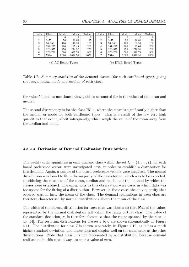
60 CHAPTER 4. ANALYSIS OF BOARD DEMAND
Index Class Mode Mean Median1 0 0 0 02 1–75 50 28.66 253 76–150 100 110.38 1004 151–225 200 195.49 2005 226–375 250 274.92 2506 376–750 500 525.70 5007 751+ 1 000 1 826.50 1 050
(a) AC Board Types
Index Class Mode Mean Median1 0 0 0 02 1–75 50 26.81 203 76–150 100 108.93 1004 151–225 200 193.04 2005 226–375 250 276.31 2606 376–750 500 510.79 5007 751+ 1 000 1 410.91 1 000
(b) DWB Board Types
Table 4.7: Summary statistics of the demand classes (for each cardboard type), givingthe range, mean, mode and median of each class.
the value 50, and as mentioned above, this is accounted for in the values of the mean andmedian.
The second discrepancy is for the class 751+, where the mean is significantly higher thanthe median or mode for both cardboard types. This is a result of the few very highquantities that occur, albeit infrequently, which weigh the value of the mean away fromthe median and mode.
4.3.2.3 Derivation of Demand Realisation Distributions
The weekly order quantities in each demand class within the set K = {1, . . . , 7}, for eachboard preference vector, were investigated next, in order to establish a distribution forthis demand. Again, a sample of the board preference vectors were analysed. The normaldistribution was found to fit in the majority of the cases tested, which was to be expected,considering the closeness of the mean, median and mode, and the method by which theclasses were establised. The exceptions to this observation were cases in which data wastoo sparse for the fitting of a distribution. However, in these cases the only quantity thatoccured was, in fact, the mean of the class. The demand realisations in each class aretherefore characterised by normal distributions about the mean of the class.
The width of the normal distribution for each class was chosen so that 95% of the valuesrepresented by the normal distribution fall within the range of that class. The value ofthe standard deviation, σ, is therefore chosen so that the range spanned by the class is4σ [54]. The resulting distributions for classes 2 to 6 are shown schematically in Figure4.11. The distribution for class 7 is shown separately, in Figure 4.12, as it has a muchhigher standard deviation, and hence does not display well on the same scale as the otherdistributions. Note that class 1 is not represented by a distribution, because demandrealisations in this class always assume a value of zero.

4.3. Demand Distributions 61
4.3.2.4 Derivation of Transition Probabilities
Based on the demand classes established in §4.3.2.2, the following analysis was conductedfor each board preference vector, based on the historical demand data available9. Thenumber of transitions from each demand class j ∈ K to each other demand class m ∈ Kwas calculated. This was expressed as a fraction of the total number of incidents of thedemand in class j. These are conditional probabilities (with the condition being thatdemand class m is the current one realised) that quantify the likelihood that demandclass j will be the next one realised. The conditional probabilities therefore determinethe transition between states in the Markov demand process. These computations wereconducted for each initial demand class j of each of the board preference vectors. Thetransition probabilities for one of the board preference vectors is given, as an example,in Table 4.8.
Demand ToState j = 1 j = 2 j = 3 j = 4 j = 5 j = 6 j = 7
m = 1 0.49 0.11 0.04 0.09 0.04 0.09 0.13F m = 2 0.38 0.63 0.13 0.13 0.00 0.63 0.25r m = 3 0.50 0.00 0.00 0.00 0.00 0.00 0.00o m = 4 0.25 0.25 0.08 0.42 0.00 0.00 0.00m m = 5 0.5 0.5 0.00 0.00 0.00 0.00 0.00
m = 6 0.29 0.29 0.14 0.14 0.00 0.00 0.14m = 7 0.64 0.07 0.00 0.00 0.00 0.14 0.14
Table 4.8: The transition probabilities for board preference vector 6, indicating the prob-ability of a transition from each state to each other state.
A complete list of the resulting transition matrices is included in a CD inside the backcover of this thesis.
4.3.2.5 Derivation of Conversion Factor Probabilities
As discussed, each sheet order is converted to an order for a board preference vector.However, in this process the information as to how many sheets can be produced fromeach board is lost. This number may be different for each sheet that is associated with aspecific board preference vector. Hence, each order placed for a certain board preferencevector may be associated with different sheet–to–board conversion factors.
One intuitive way of countering this information loss would be to expand the boardpreference vectors, in order to retain this information. This could be achieved by includinga conversion factor for each sheet associated with the board preference vector, for eachboard in the vector, so that orders for the same combination of boards, but differentconversion factors, are distinct entries. However, this would increase the number of boardpreference vectors from 386 to 781. Such an increase is not desirable, as it greatly reducesthe number of historical demand entries associated with each board preference vector,thereby decreasing the accuracy of the probabilities derived, based on the historical data.
9This was implemented by means of programs written by the author in Microsoft Access and VisualBasic, and the relevant source code is given in §C.4 of Appendix C.

62 CHAPTER 4. ANALYSIS OF BOARD DEMAND
The eventual approach taken was therefore not to include the sheet–to–board conversionfactors in the board preference vectors, but rather to derive a probability distribution forthe sheet–to–board conversion factors. In this way, when a demand for a board preferencevector is realised, the corresponding sheet–to–board conversion factor for each board inthe board preference vector is derived from the probability distribution.
This was achieved, again by analysis of the historical data10, as follows. The averagesheet–to–board conversion factor per week, for each board in each board preference vec-tor, was calculated. The averages were weighted to take into account the quantity ofeach order. The number of occurrences of each of the sheet–to–board conversion factoraverages, for each board in each board preference vector, was then divided by the to-tal number of demand occurrences for that board preference vector. The probability ofoccurrence of the first few sheet–to–board conversion factors for one of the board prefer-ence vectors is given, as an example, in Table 4.9. A complete list of the sheet–to–boardconversion factor probabilities for all board preference vectors is included on a CD insidethe back cover of this thesis.
The notation of the sheet–to–board conversion factor m(i,β) is amended to m(i,β)t , as the
board factor now represents the probable number of sheets, optimally manufactured byboard preference vector vi, that may be produced from board β in week t.
Board Index Factor Probability1 4.00 0.311 5.33 0.031 6.00 0.031 6.26 0.031 6.58 0.031 6.67 0.031 7.45 0.061 7.57 0.031 8.00 0.402 2.00 0.962 4.00 0.043 2.00 0.033 4.00 0.313 5.33 0.033 6.00 0.033 6.26 0.033 6.58 0.033 6.67 0.033 7.45 0.063 7.57 0.033 8.00 0.40
Table 4.9: The entries in the board factor matrix for board preference vector 1, givingthe probability of occurrence of some potential factors for the board in each of the threepositions in the board preference vector.
10This was implemented by means of programs written by the author in Microsoft Access and VisualBasic, and the relevant source code is given in §C.5 of Appendix C.

4.4. Chapter Summary 63
4.4 Chapter Summary
The historical data available from Clickabox was analysed in this chapter, in order todetermine an optimal set of stock boards to be kept in inventory, and to characterisethe nature of the demand process for the purposes of inventory modelling. An ABCclassification was conducted in §4.2.1, the results of which showed board types AC andDWB to be the most important board types to be kept in stock, because of their highannual usage values. The heuristic used to determine a suitable set of board dimensionsto be kept in inventory was described in §4.2.4, and the results were given and discussedin §4.2.5. The resulting suggested stock board profile has been accepted and implementedby the management of Clickabox as of March 2003. The new stock profile has provedto perform well compared to the old stock profile in terms of a reduction in wastage,as, when both stock profiles were loaded in the system, the newly suggested stock boardtypes were consistently chosen over the old stock boards to be the optimal boards ininventory to satisfy customer orders. The concept of a board preference vector, usedto incorporate the cascading product substitution that takes place at Clickabox, wasthen introduced in §4.3.1. In §4.3.2, demand classes for board preference vectors weredefined, and then two core inventory modelling processes were introduced, namely thedemand realisation process and the Markov decision process. Based on the historicaldata available, distributions were derived to model these processes. It is upon thesedistributions that the inventory model in the following chapter is built.

64 CHAPTER 4. ANALYSIS OF BOARD DEMAND
�
�����
�����
�����
�����
������
������
������
������
������
�������
� � ��������������������� ����� ��������� ��������������������������������������
!#"�$�% &�'!#"�&�'!#�($("
) *+ ,-./0,11* 2304 *45 645 76
8:9<;>=@?BADC�E�=GF�F:CH=IJ9<K@L@M�NO9<F
(a) AC board types
P
Q�P�P
R�P�P
S�P�P
T�P�P
UP�P�P
UQ�P�P
UR�P�P
US�P�P
P U V�W�X�YZX�S�V�W�U�Y�P[U�Y�U\V�W�Q�Q�Y]Q�Q�S�V�W�^�X�Y]^�X�S�V�W�X�Y�P X�Y�P�_
`#W(a�b`#b�c�d`#b�aJe c�d
f gh ijklminng opmq gqr sqr ts
u:v<w>x@yBz|{H}�xG~�~:{Hx�Jv<�@�@���Ov<~
(b) DWB board types
Figure 4.10: Graphical depiction of summary statistics for each demand class, showingthe correlation between the mean, mode and median of each class.

4.4. Chapter Summary 65
200 400 600 800
0.005
0.01
0.015
0.02
0.025Cl.2
Cl.3
Cl.4
Class¬ 5 ®
Class¬ 6 ®
Figure 4.11: The normal distributions of demand classes 2 to 6, indicating the range ofeach class. Demand realisations in class 1 assume the value of zero. The demand distri-bution for class 7 has a much higher standard deviation and so is illustrated separately.
1000 2000 3000 4000 5000
0.0001
0.0002
0.0003
0.0004
0.0005Class¬ 6 ®
Class7 �
Figure 4.12: The normal distribution of demand class 7, indicating the range of the class.

66 CHAPTER 4. ANALYSIS OF BOARD DEMAND

Chapter 5
Inventory Model
The objective in this chapter is to design a strategic mathematical model in order to aidthe inventory manager when replenishing stock at Clickabox. A theoretical optimal controlpolicy is defined for the case of non–stationary, partially observed demand, modelled asa finite state Markov Chain. A sub–optimal control policy, which is more practical withrespect to computational requirements, is then developed. The objective of this policy isthe minimization of expected tied–up inventory capital subject to an acceptable level ofoffcut wastage costs, whilst satisfying the given service level requirements.
5.1 General Modelling Assumptions
The following modelling assumptions will be assumed to hold throughout this chapter.
1. The financial year is divided into 52 one–week time periods. These week periods areindexed by the set T = {0, . . . , 51}, with period 0 being the week 1 — 7 February,period 1 being the week 8 — 14 February and so on, until period 51, which is theweek 25 — 31 January. The planning horizon for the model is one year.
2. Boards are ordered at the start of a one–week time period, and are delivered atthe start of the week, the lead time number of weeks later. Lead time for deliveryof boards from suppliers is constant (l = 2 weeks). The lead time in reality isvariable, but not highly variable (typically between seven and ten working days).This assumption simplifies the modelling process.
3. Unsold boards at the end of the one–year planning horizon maintain their value forfuture periods.
4. Demand for any box type during any given week arises from one of a number ofprobability distributions. The distribution changes randomly from one week to thenext. At the beginning of any given week it is not certain from which distributionthe demand will be generated for that week. However, the transition probabilitiesfor demand from one week to the next are known and fixed.
67

68 CHAPTER 5. INVENTORY MODEL
5. If the optimal board is not available to satisfy an order, the next best board isused. This is termed stock cascading, as discussed before. The cost of customerdissatisfaction is represented by the increased wastage cost sustained when using asub–optimal board. The wastage cost is in reality sustained by the customer andnot by Clickabox, but for modelling purposes will represent the cost of shortage.
6. In the case of no suitable board being available to produce an order, i.e. not evena substitute board is available, demand is completely backordered. As discussed inChapter 4, this will result in a high shortage cost being incurred.
7. Raw materials are available for production as soon as they arrive at the warehouse.There are at most two raw materials deliveries to the factory per day [70]. Thedeliveries are offloaded directly into the warehouse and the boards are markedavailable for use as soon as the delivery is recorded into the system. Under normalcircumstances this will happen immediately.
8. Income that is redeemed through the processing or recycling of offcuts is neglected.This is justified as the income from recycling is approximately R1 845 per month,compared to a turnover of R450 000 — R600 000 per month in 2002.
9. Orders are assumed to be fulfilled as soon as production is complete, i.e. deliveryis assumed to take place on the same day that an order is ready. This is normallythe case [70], the exceptions are a result of poor production planning and do notfall within the scope of this thesis.
10. No raw materials are damaged in storage. Storage damage occurs when piles arestacked too high and fall over, usually as a result of the warehouse being too full.It is assumed that, given the cost associated with holding stock included in theinventory model, the occurrence of this will be minimal. It is, in fact, estimated bymanagement that less than 0.1% of the stock in inventory at Clickabox is lost dueto damage in storage [70].
11. Fulfillment of orders is dependent only on availability of stock, i.e. machine break-downs and labour shortages do not influence the production schedule. As in (8)above, exceptions to this assumption fall beyond the scope of this thesis.
5.2 Spatial Constraints
Spatial constraints for the inventory model will be establised as firstly the volume ofstorage space available, and then as an approximate number of boards that can be storedin the available space.
Available space is calculated in cubic meters. There is a restriction on the height to whichboards may be stacked in the warehouse, for convenience purposes and to prevent theboards from being damaged due to pressure in the stack. The maximum height to whichboards should be stacked is 3.2 metres. Allowance must also be made for loading andmanoeuvering of forklifts, so 45 metres of the length of the storage area and 11 metres

5.2. Spatial Constraints 69
of its width are used for storage. Available space in the raw materials store is therefore1 584m3.
The approximate number of boards that can be stored in this space is now calculated.The maximum length of boards is 2.49m and the maximum width is 2.38m, due toconstraints on the machinery used to process orders. Hence the available space allowsfor 72 bays in which to store different board dimensions, 18 lengthwise and 4 widthwisein the storeroom. The bays are divided proportionately between the AC and the DWBboards, according to the number of sizes of each cardboard type kept in stock. Thisresults in 44 bays for the AC boards, and 28 bays for the DWB boards. Each bay holdsonly one type of board; the more popular board dimensions are allocated more than onebay. As discussed in Chapter 4, the stock boards are ranked according to annual usuagevalue. It is assumed that the 16 most popular AC board dimensions (termed the Rank A
board types in Table 4.2) are allocated two bays each, and the remaining 12 AC boardtypes (termed the Rank B board types in Table 4.2) are allocated one bay each, to makeup the total of 44 bays allocated for storage of the AC board types. Similarly, the tenDWB Rank A board types are allocated two bays each, and the remaining eight DWBRank B board types are allocated one bay each, to make up the total of 28 bays allocatedfor storage of the DWB board types.
AC boards are 4.4mm thick, while DWB boards are 7.6mm thick. The number of ACboards that can be stored in each bay is therefore 3.2m ÷ 0.004 4m = 727 boards, andthe number of DWB boards that can be stored is 3.2m ÷ 0.007 6m = 421 boards. Theconstraint on the number of boards of each type that may be stored in the availablespace, dependent on board type and rank, is defined as η$
(z), where $ is the rank (either
A or B), and z is the board type (either AC or DWB). The current constraints on thenumber of each board type and rank that may be held in inventory are given in Table5.1(a).
If the threshold values given in Table 5.1(a) are exceeded, the viability of renting addi-tional storage space must be investigated.
ηA(AC)
1 454
ηB(AC)
727
ηA(DWB)
842
ηB(DWB)
421
(a) Current Position
ηA(AC)
2 182
ηB(AC)
727
ηA(DWB)
1 263
ηB(DWB)
421
(b) Upper Limit
Table 5.1: Spatial constraint for each board type and rank, given as the number ofboards, that can be stored in inventory. Table (a) gives the constraints based on thecurrent storage position, and Table (b) gives the so–called upper limit, which representsthe approximate number of boards which could be stored in inventory were all viableavailable space to be used for storage.
The current wastage recovery area has a usable area of 11 metres by 23 metres, whichpotentially allows for an additional 20 bays for AC boards and an additional 12 bays for

70 CHAPTER 5. INVENTORY MODEL
DWB boards, in other words an additional 14 540 AC and 5 052 DWB boards may bestored in this area, if required, at an additional cost. It is assumed that any additionalstorage space will be occupied proportionally between AC and DWB boards. The ap-proximate number of boards which could then be kept in storage, based on one bay forthe rank A boards of both board types, are given in Table 5.1(b). These are the valuesthat will be used in the optimisation model as the upper limit of the order–to level.
5.3 Board Holding costs
Three categories of holding costs (dependent on the quantity of boards kept in the in-ventory) have been identified. These are the rental cost of floorspace in the factory, theopportunity cost of tied–up capital, and the cost of insurance.
5.3.1 Rental Cost
The building in which the Clickabox factory is housed is owned by the director of thefactory, and Clickabox pays a monthly rental to him at a market–related rate. This is afixed rental charge, independent of inventory levels. However, an increase in the amountof space utilised results in decreased manoeuvrability of the forklifts in the warehouse,and therefore an increase in the time required to fetch raw materials for production. Themodelling of rental costs therefore takes into account the positive correlation between theamount of stock held and the cost of holding the stock. This is done as follows.
The proportion of total rental cost attributed to the storage area is given by
Rs =As
At
Rp
=1 584m2
2 518.5m2R415 400
= R261 264.09,
where At represents the total floor area of the factory, As represents the floor area of thestorage space (as calculated in §3.2), and Rp the total rent paid per annum.
Rental cost for the storage area per volume of stock per week is now calculated as
Rc =Rs
52Ash′
=R261 264.09
52 weeks × 1 584m2 × 3.2m
= R0.99 per m3 per week, (5.1)
where h′ represents the height to which boards may be stacked.
This rate applies to the available space in the raw materials store, which can store approx-imately 31 988 AC boards and 11 788 DWB boards (as calculated in §5.2). If inventory

5.3. Board Holding costs 71
levels exceed these thresholds, an additional cost will be incurred, as it will be necessaryto utilize the current waste recovery area for the storage of stock. The waste recoveryarea currently generates an income of approximately R1 845 per month, or R461.25 perweek [75]. The additional cost incurred is the opportunity cost of converting the spaceutilized for this recovery operation to storage space for inventory. Space available in thisarea is sufficient for the storage of a further 14 540 AC and 5 052 DWB boards.
Boards vary in dimension, so rental cost per board is different for each board kept instock, and is given by the cost per cubic metre, Rc, multiplied by the volume of theboard. There are 28 AC board types and 18 DWB board types kept in inventory fromwhich sheets may be produced; let the sets BAC = {1, . . . , 28} and BDWB = {29, . . . , 46}index these board types respectively, and let B = BAC ∪ BDWB.
The rental cost function for board β ∈ B during week t is given by x(β)t Rcv
(β), where x(β)t
is the number of boards of type β in inventory during week t, where v(β) is the volumeper board of type β and Rc is the rental cost per volume of stock, as calculated in (5.1).The total rental cost is therefore given by
RT =
{
∑46β=1 x
(β)t Rcv
(β), if x(β)t ≤ η
$β
(zβ) for all β ∈ B∑46
β=1 x(β)t Rcv
(β) + R461.25, otherwise,(5.2)
where $β ∈ {A, B} denotes the rank and zβ ∈ {AC, DWB} denotes the type of the boardindexed by β ∈ B. In other words, the additional rental cost for the waste recovery areais incurred if the inventory level of any of the stock board types exceeds the limit η
$β
(zβ)
for any board β ∈ B, as shown in Table 5.1.
The values of v(β), the volume of each board β, are listed in Tables A.1 and A.2 ofAppendix A.
5.3.2 Opportunity Cost
The loss due to capital tied up in stock is an opportunity cost, calculated in terms of theinterest that would have been earned, were that money invested in the bank. Tied–upcapital is therefore directly proportional to the cost of the raw materials. For a rawmaterial purchase price of p(β) [Rands per board of type β] and a cost–of–capital–per–week rate c, the opportunity cost of keeping one unit of board β in stock for one week isgiven by cp(β). The purchase cost p(β) is given by
p(β) =
{
A(β) × 2.54, if zβ = ACA(β) × 4.46, if zβ = DWB,
(5.3)
where A(β) denotes the surface area of board β.
The total tied–up capital during week t is therefore
P =46∑
β=1
cp(β)x(β)t
= 2.54c28∑
β=1
A(β)x(β)t + 4.46c
46∑
β=29
A(β)x(β)t . (5.4)

72 CHAPTER 5. INVENTORY MODEL
5.3.3 Insurance Cost
Insurance costs are calculated on the total value of stock and machinery housed in thefactory. This amount is reviewed annually, and the value of stock insured is calculatedbased on the estimated average stockholding for the year to come.
However, it is practically very difficult to link a variation in the number of boards instock month by month to monthly insurance costs. The monthly insurance premium is,in fact, predetermined, and the number of boards insured at any stage depends on thecomposition of the inventory (in terms of board sizes, types and numbers) during thesame month of the previous financial year, and the cost price of each board in stock.
This cost variation is negligible compared to the opportunity cost of the capital investmentin the inventory. Insurance cost will therefore be considered a fixed cost for modellingpurposes.
Current insurance rates are approximately R2 280 per month, i.e. R570 per week, forinsurance on a replacement value of R500 0001 of stock in inventory.
5.3.4 Total Holding Costs
The unit holding cost for board β is therefore
h(β) = x(β)t
(
Rcv(β) + cp(β)
)
+R570.00
46, (5.5)
and the total holding cost is given by
hT = P + RT + R570.00, (5.6)
where P and RT are given in (5.4) and (5.2) respectively.
5.4 Cascading Shortage Costs
Shortage costs are difficult to estimate, due to the complicated nature of customer senti-ment. This cost should incorporate bad sentiment if customers’ orders are not met withinthe promised lead time, and also if the orders are met, but at a high cost due to the use ofsub–optimal boards, with much wastage. In the case of Clickabox, the cascading shortagecost s(β) is formulated as the expense incurred due to this wastage (although it is, in fact,incurred by the customer and not the factory itself).
This cost may be estimated by
s(β) =A(k) − A(β)
A(β)p(β), (5.7)
1This replacement value was estimated by the management of Clickabox, after inspection of theaverage value of stock in inventory during 2002, for the purposes of determining the insurance premiumsfor 2003 [70].

5.5. Service Level Measures 73
if board type k is the board type used instead of the optimal board type β, where p(β) isthe purchase cost of board type β, and A(β) is the area of board type β as before.
However, the actual shortage cost depends on the composition of the board preferencevectors and on the inventory levels, and calculation of the actual shortage cost thereforerequires a knowledge of a number of issues not yet addressed. For the purposes of cal-culating service levels, however, the simplistic cascading shortage cost estimate in (5.7)is used. This concept will be extended later to comprise a wastage cost defined for eachboard in each board preference vector, and a shortage cost dependent on a combinationof these wastage costs and the inventory levels of each board in the board preferencevector.
In the case of no boards being available to satisfy an order, the order is backlogged, anda fixed stockout penalty cost is incurred.
5.5 Service Level Measures
In this section the choice of service level will be discussed, beginning with a clarification ofthe difference between service level and fill rate. A service level is the required percentageof order cycles during the year, during which there will be no shortages. A fill rate is therequired percentage of units demanded that will be in stock when needed. The fill rateis generally significantly higher than the service level.
An algebraic computation can be performed to determine an appropriate service levelα(β) for each board type β ∈ B, taking into account the trade–off between holding costh(β) and shortage costs s(β), and the frequency at which the factory is exposed to thepossibility of running out of stock [16]. This is calculated individually for each boardtype in the four steps outlined below.
Step 1: Computing the optimal number of stockouts each year, S∗(β). This is achieved bytaking the ratio of the annual holding cost h(β) of board type β to the shortage cost s(β)
for board type β, because if the holding cost is relatively high compared to the shortagecost, the factory should plan on stocking out relatively often, since the cost of carryinghigh safety stocks would be prohibitive. Conversely, with relatively high shortage costs,the factory may plan for a low probability of stocking out by carrying high safety stock.Therefore the planned number of stockouts per year is given by
S∗(β) =h(β)
s(β), β ∈ B. (5.8)
Step 2: Computing the number, κ(β), of order cycles each year. This is given by theaverage annual demand D(β) for boards of type β divided by the quantity ordered duringeach cycle, that is
κ(β) =D(β)
q(β), β ∈ B. (5.9)
In the case of a fixed review problem, κ(β) is the number of review periods in a year. Thisindicates the potential number of exposures to stockout the factory will experience for
74 CHAPTER 5. INVENTORY MODEL
board β each year.
Step 3: Computing the probability S(β)
of a stockout during each order cycle given theoptimal number of stockouts computed in (5.8) and the number of exposures to stockoutsgiven by (5.9). Suppose, as an example, the optimal number of stockouts is one everytwo years, and there are five order cycles a year. Then there are ten order cycles in thetwo year period. If there is one stock out during these ten order cycles, there is a one inten, or 10%, chance of stockout during the order cycle. In general this probability is
S(β)
=S∗(β)
κ(β), β ∈ B. (5.10)
Step 4: Deriving the service level, α(β), as the probability of not stocking out of boardβ during each order cycle, i.e.
α(β) = 1− S(β)
= 1−S∗(β)
κ(β)
= 1−h(β)q(β)
s(β)D(β), β ∈ B, (5.11)
by utilisation of (5.8)–(5.10).
A major assumption of this computation is that holding and shortage costs are linear,i.e. carrying 100 boards costs twice as much as carrying 50 boards, and a stockout of fiveboards costs five times as much as a stockout of one board.
Service levels calculated as above will almost always be lower than intended, as thecalculation does not take into account all the issues that affect customer perceptions,such as the length of stockout periods. Plossl and Wight (1967, [59]) suggest that theservice level should be inflated to compensate for this phenomenom. However, they donot suggest by how much.
In view of the above discussion, the specification by the management of Clickabox that“95% of orders should be met within the specified time” is, in fact, a fill rate.
The above method was used to calculate a theoretically appropriate service level for eachstock board at Clickabox.
A number of additional assumptions are made for the purposes of this calculation:
1. Rental cost and the cost of insurance are assumed to be fixed costs; holding cost istherefore only the opportunity cost defined in (5.4). Thus the assumption requiredfor the service level computation, i.e. that the holding cost is linear, is assumed tohold.
2. The cost–of–capital–per–week rate is derived from the prime interest rate in SouthAfrica at time of writing, namely 17% per annum [62].
3. The shortage cost, defined in (5.7) are also assumed to be linear for the purpose ofthe service level computation.

5.5. Service Level Measures 75
4. It is assumed that the sub–optimal board used will be the board type, amongstthose having each dimension greater than or equal to those of the optimal boardtype, that is closest in area to the optimal board type. This is a ‘best case’ scenario,as this ‘second best’ board will not in reality always be available, and a differentboard, associated with a higher wastage cost, would have to be used. The readershould note that this is a simplifying assumption made in order to define a simplelinear shortage cost per board for the purposes of the service level calculations only.As mentioned in §5.4, the modelling of the total shortage cost in a realistic manneris more complex and will be discussed in detail later.
The ‘sub–optimal’ board types were determined by means of a program written by theauthor in Visual Basic [50] and Microsoft Access [49]2. The program also takes intoaccount the possibility of using more than one board type, for example board type AC2 300 × 1 200 cannot be substituted by a single board type, as there is no other stockboard type of length 2 300 or greater. This board is most efficiently substituted by twoboards of type AC1 250 × 1 300, joined lengthwise. The set of board types and theirsub–optimal board types are given in Appendix A.
The optimal service level is now calculated for board type AC 1 260×2 300, as an example.
Step 1: The optimal number of stockouts each year is given by
S∗(β) =h(β)
s(β)
=p(β)c
s(β)(Assumption (1), Equation (5.4))
= p(β)cA(β)
(A(k) − A(β))p(β)(Assumption (3), Equation (5.7))
= 0.17×2.898m2
0.23m2, (Assumption (3))
= 2.14.
Thus the optimal number of stockouts is approximately two each year.
Step 2: The order quantity during each cycle is 1 000, as discussed in §3.5.1. The numberof order cycles each year is then
κ(β) =D(β)
q(β)
=38 315
1 000= 38.32.
This gives an indication of the number of exposures to stockouts each year.
Step 3: The probability during each order cycle of a stockout is
S(β)
=S∗(β)
κ(β)
= 0.055 8.2The relevant code is given in §C.2 of Appendix C

76 CHAPTER 5. INVENTORY MODEL
Step 4: The probability of not stocking out is therefore
α(β) = 1− S(β)
= 0.944 2.
Index Board Type Stockouts Order cycles Stockout probability Theoreticalper year per year per order cycle Service Level
1 AC 1 030 × 2 370 0.58 12.21 0.05 95.22%2 AC 1 260 × 2 300 2.14 38.32 0.06 94.41%3 AC 1 280 × 1 300 1.97 11.27 0.17 82.54%4 AC 1 330 × 2 370 1.74 5.93 0.29 70.67%5 AC 1 360 × 2 300 1.60 31.19 0.05 94.87%6 AC 1 380 × 1 310 1.01 6.91 0.15 85.36%7 AC 1 460 × 2 370 0.84 24.55 0.03 96.59%8 AC 1 470 × 1 480 2.75 9.57 0.29 71.23%9 AC 1 500 × 1 540 0.93 5.04 0.18 81.60%10 AC 1 510 × 1 810 0.54 46.06 0.01 98.82%11 AC 1 530 × 1 380 0.54 34.74 0.02 98.43%12 AC 1 550 × 1 020 1.15 5.93 0.19 80.59%13 AC 1 680 × 1 080 1.16 17.08 0.07 93.23%14 AC 1 720 × 1 210 0.81 33.55 0.02 97.58%15 AC 1 800 × 1 200 1.03 5.31 0.19 80.64%16 AC 1 860 × 1 000 1.17 10.48 0.11 88.87%17 AC 1 860 × 1 490 0.71 52.06 0.01 98.64%18 AC 1 910 × 1 880 0.47 29.15 0.02 98.38%19 AC 2 000 × 1 400 0.75 6.48 0.12 88.43%20 AC 2 030 × 1 240 0.96 25.41 0.04 96.22%21 AC 2 110 × 1 010 0.71 24.23 0.03 97.06%22 AC 2 110 × 1 680 1.55 29.78 0.05 94.79%23 AC 2 200 × 1 200 2.70 4.02 0.67 32.79%24 AC 2 260 × 1 520 1.17 18.21 0.06 93.56%25 AC 2 260 × 2 160 0.28 27.65 0.01 98.99%26 AC 2 300 × 1 220 3.05 10.95 0.28 72.16%27 AC 2 300 × 1 710 0.44 21.89 0.02 98.01%28 AC 2 370 × 1 250 1.38 5.17 0.27 73.34%
Table 5.2: The optimal number of stockouts each year (S∗(β)), the number of order cycles
a year (κ), the probability during each order cycle of a stockout (S(β)
), and the theoreticalservice levels for each of the suggested AC Stock Boards to be kept in inventory.
The theoretical service level for board type AC 1 260 × 2 300 is therefore 94.42%. Thetheoretical service levels for the other AC boards, calculated by the process detailedabove, are given in Table 5.2.
Note that for the board AC 2 200×1 200 a very close substitute, namely AC2 300×1 220,is available with only 5.92% wastage. The cost of shortage is therefore quite low, andso the optimal number of stockouts a year is high. This, along with a low demand andtherefore few order cycles a year, result in a service level of only 32.79%. In contrast,board AC1 910× 1 880 has a 98.38% service level as the closest substitute is board typeAC2 260× 2 160, with a large wastage of 26.44%.
The average theoretical service level for AC boards is 87.61%, and the average theoreticalservice level for DWB boards is 90.68%. The theoretical service levels for the DWB boardsare given in Table 5.3.
The fill rate used in this study is as specified by the factory director. There is currentlyno record kept of the factory’s performance in terms of wastage loss and orders being

5.6. Optimal Control Policy 77
Index Board Type Stockouts Order cycles Stockout probability Theoreticalper year per year per order cycle Service Level
29 DWB 1 050 × 1 980 0.20 5.67 0.04 96.39%30 DWB 1 170 × 1 310 1.22 5.57 0.22 78.14%31 DWB 1 230 × 1 420 0.72 5.28 0.14 86.37%32 DWB 1 270 × 1 700 0.64 9.07 0.07 92.98%33 DWB 1 410 × 1 940 0.44 14.62 0.03 97.02%34 DWB 1 480 × 1 310 2.10 14.25 0.15 85.30%35 DWB 1 530 × 1 370 0.45 6.04 0.07 92.51%36 DWB 1 670 × 1 010 0.57 10.83 0.05 94.77%37 DWB 1 780 × 1 620 0.76 12.26 0.06 93.77%38 DWB 1 820 × 2 090 0.53 17.88 0.03 97.01%39 DWB 1 870 × 1 350 1.05 21.80 0.05 95.20%40 DWB 2 010 × 1 460 0.84 9.97 0.08 91.54%41 DWB 2 030 × 1 080 0.35 6.29 0.06 94.37%42 DWB 2 150 × 1 640 1.10 9.21 0.12 88.09%43 DWB 2 270 × 1 430 0.67 7.13 0.09 90.64%44 DWB 2 300 × 2 180 0.27 6.10 0.04 95.54%45 DWB 2 330 × 2 000 0.27 4.94 0.05 94.56%46 DWB 2 410 × 1 690 2.82 8.84 0.32 68.06%
Table 5.3: The optimal number of stockouts each year (S∗(β)), the number of order cycles
a year (κ), the probability during each order cycle of a stockout (S(β)
), and the theoreticalservice levels for each of the suggested DWB Stock Boards to be kept in inventory.
met; these figures were estimated by two methods. The first was by consultation withthe director of the factory, who is involved with all the operational aspects of the factoryand is perceived to have a good idea of the situation. The estimates provided by thefactory director were averages for all board types. The second method was by analysisof data of orders placed and met during the time period 1 February 2001 — 31 January2003. This was done for AC and DWB board types separately. These estimates are givenin Table 5.4.
Opinion of director Observed values Observed values RequiredAll AC DWB All
Orders met on time 90% ≥95%Orders made with ideal board 80% 72.13% 74.27% n\aOff–cut wastage 30% 29.76% 29.68% ≤15%
Table 5.4: Performance Measures
Note that, due to the nature of the data available, the number of orders processed withideal board is underestimated, as it is obtained by a count of only those orders made withmore than one board type, and does therefore not include those orders filled completelywith a sub–optimal board.
5.6 Optimal Control Policy
In this section an inventory model for Clickabox is derived for the case of non–stationary,partially observed demand with a positive lead time, l. The demand during each weekmay be generated by any one of a number of probability distributions. The probability

78 CHAPTER 5. INVENTORY MODEL
distribution for the demand is determined by a Markov decision process. An expressionfor the expected inventory cost for each week is derived, and then an optimal controlpolicy, which minimises this cost subject to the service levels derived in §5.5, is found.
5.6.1 Board Preference Vector Demand
The demand classes were defined in Chapter 4 to be seven ranges of values which maybe assumed by the demand process (see Figure 4.7). For the remainder of this chapterthe terms demand state and demand class will be used interchangeably, as each demandclass represents a state in the Markovian process. The demand state process for eachboard preference vector, in other words the sequence of classes that may be taken on bythe demand distribution for each board preference vector vi, is not known with certainty.It is modelled as a finite state Markov Chain, which may take on any one of a number ofstates during each week t, indexed by the set K = {1, 2, . . . , 7}.
The demand class of board preference vector vi during week t is denoted by
dvit , i ∈ V, t ∈ T . (5.12)
The Markov process is governed by a transition probability matrix, Pvi. Each time thesystem is in class k (that is, if d
vit = k for some time t ∈ T ), there is a fixed probability
Pvi
k,j (the entry in row k and column j of a matrix of probabilities, Pvi) that it will next be
in class j (that is, dvi
t+1 = j, t ∈ T \ {51}). These values, Pvi
k,j, are known as the transitionprobabilities of the Markov chain,
Pvi
k,j = Pr[
(dvi
t+1 = j)|(dvit = k)
]
. (5.13)
The transition probabilities satisfy the conditions
Pvi
k,j ≥ 0 and7∑
j=1
Pvi
k,j = 1, k, j ∈ K, i ∈ V. (5.14)
The transition probability matrices Pv1, . . . ,Pvµ are themselves assumed to be stationary.Stationary demand for the board preference vector vi may be modelled by taking Pvi = I,the identity matrix, whilst trends in demand for board preference vector vi may bemodelled by taking Pvi as an upper or lower triangular matrix.
The demand state process is partially observed and the observed demand for board pref-erence vector vi up to the start of week t ∈ T is defined as the measurement process{w
vi
0 , . . . , wvi
t−1}. The observed demand wvit for board preference vector vi during week t
is the sum of all order quantities of orders placed during week t for sheets in S that maybe produced by boards indexed in vi. It is assumed, for expected optimal replenishmentpurposes, that the best board in each board preference vector, that is the board vi,1, willbe used to fulfil an order. However, the inventory cost function will take into accountthe shortage cost incurred when the demand must, to some extent, be met by boards vi,2
and vi,3, due to stockout.
As discussed in Chapter 4, the demand realisation process is characterised by a normaldistribution about the mean of each class. The demand realisation during a period

5.6. Optimal Control Policy 79
is conditional on the current demand class. If dt = k, the probability distribution ofdemand for board preference vector vi during week t is given by
Pr[(wvit = z)|(dt = k)] = r
vi
k,z, k ∈ K, t ∈ T , z ∈ {0} ∪ R+, i ∈ V. (5.15)
5.6.2 Inventory Position
The quantity of the order placed by Clickabox at its suppliers during week t for board βis denoted by q
(β)t . The inventory position for board β at the start of period t is defined
as the net inventory level x(β)t (on hand inventory less backorders) added to the stock on
order at the beginning of week t, that is
u(β)t = x
(β)t +
l∑
f=1
q(β)t−f , t ∈ T , β ∈ B. (5.16)
Here q(β)−1 , q
(β)−2 , . . . , q
(β)−l are assumed to represent orders placed during the l weeks immedi-
ately prior to the one year time window for which an optimal inventory policy is sought.All orders placed within the lead time number of weeks before any week t are included inthe inventory position, as the demand considered in the inventory model is the lead timedemand. Under the assumption of timely delivery of raw materials orders, all these orderswill arrive within that lead time number of weeks, as measured from week t onwards.
The prior distribution, Πvit , is a rectangular matrix characterising the current belief of
the distribution of the demand state dvit , given the information available up to the start
of week t, that is
Πvi
k,t = Pr[(dvit = k)|It
vi ], t ∈ T , k ∈ K, i ∈ V, (5.17)
where Ivit is the vector of information available at the start of week t for board preference
vector vi. The initial prior distribution, Πvi
k,0, is assumed to be externally specified, based
on market analysis and industry knowledge. The information vector Ivit is defined as
Ivi
0 = (Πvi
1,0, Πvi
2,0, . . . , Πvi
7,0), (5.18)
together with
Ivit =
uvi,1
0 . . . uvi,1
t−1
uvi,2
0 . . . uvi,2
t−1
uvi,3
0 . . . uvi,3
t−1
wvi
0 . . . wvi
t−1,
, i ∈ V, t ∈ T \ {0} . (5.19)
At the start of any week t, the previous values of the order quantities placed, (q(β)t−1, q
(β)t−2
, . . . , q(β)t−l), the current inventory level (x
(β)t ) and the current inventory position (u
(β)t ) are
assumed to be known for each board β ∈ B. Also known are the values of the priordistribution Π
vi
j,t and the previous demand observations in the information matrix Ivit .
As discussed, optimal inventory management should allow for the best board associatedwith a sheet to be available, on expectation. However, as a result of fluctuations in the

80 CHAPTER 5. INVENTORY MODEL
actual demand this will not always be the case in reality. Observed demand for a boardduring a week is the sum of the observed demand for each board preference vector inwhich that board is the first choice, referred to as first level demand, added to the sum ofthe vector demands where that board was a second choice (which could not be satisfiedby the first choice board), referred to as second level demand, and similarly where it wasthe third choice, called the third level demand.
In order to determine the realised demand for a board, it must be decided how availablestock of a board will be allocated to board preference vector demand. In other words, ifthere is insufficient stock of a board to fill all the demand for which it is the optimal board,it must be decided which of the board preference vector demands will be supplied by thefirst choice board. The remainder of the demand will be filled by the second or thirdchoice board. It is necessary to allocate available stock of a board to a specific boardpreference vector demand as the sheet–to–board conversion factors differ for differentboards in a board preference vectors. As a result, different quantities of each board inthe board preference vector would be required to fill a demand.
The allocation is based on the wastage cost, associated with each board in each boardpreference vector, incurred when a sub–optimal board is used. For the purpose of thisthesis, a greedy algorithm was adopted, which attempts to minimise the wastage costincurred by different allocations. Hence board allocation is conducted such that availablestock of the first choice board is first allocated to the board preference vector for whichthe wastage cost of using the second choice board is the highest. Similarly, available stockof the second choice board is first allocated to the board preference vector for which thewastage cost of using the third choice board is the highest.
Define φi,f as the wastage cost incurred, per board, when the f–th best board in boardpreference vector vi is used instead of the optimal board to meet a demand for boardpreference vector vi, where f ∈ {2, 3}. This wastage cost is given by
φi,f = (Avi,f − Avi,1)÷ Avi,1 . (5.20)
Now the realised demand for board β during week t is given by
W(β)t =
[
W(β)t,1 ; W
(β)t,2 ; W
(β)t,3
]
, (5.21)
where
W(β)t,1 =
∑
vi,1=β
wvit
m(i,β)t
(5.22)
W(β)t,2 =
b∑
k=1
∑
vi,1=k
vi,2=β
wvit
m(i,k)t
−min
wvit
m(i,k)t
, max
x(k)t −
∑
φj,2>φi,2
vj,1=k;vj,2=β
wvj
t
m(j,k)t
, 0
m(i,k)t
m(i,β)t
(5.23)

5.6. Optimal Control Policy 81
W(β)t,3 =
b∑
k=1
∑
vi,1=k
vi,3=β
wvit
m(i,k)t
−min
wvit
m(i,k)t
, max
x(k)t + max
xvi,2
t −∑
vm,1=vi,2
wvmt
m(m,vi,2)t
, 0
−∑
φj,3>φi,3
vj,1=k;vj,3=β
wvj
t
m(j,k)t
, 0
×m
(i,k)t
m(i,β)t
(5.24)
for all t ∈ T , k, β ∈ B, and i ∈ V, where m(i,β)t represents the number of sheets, optimally
manufactured by board preference vector vi, that may be produced from board β in weekt.
The rationale behind these expressions is perhaps best explained by means of an example.
Consider the board preference vectors,
v1 =
b1
b2
b4
, v2 =
b3
b1
b4
, v3 =
b3
b1
b2
, v4 =
b2
b1
b4
, v5 =
b4
b2
b1
, v6 =
b4
b3
b1
,
with demands during week t of wv1t , w
v2t , w
v3t , w
v4t , w
v5t and w
v6t respectively. Let the
inventory levels of the boards b1, b2, b3 and b4 at the start of week t be x(b1)t , x
(b2)t , x
(b3)t ,
and x(b4)t respectively. Now the first level demand for board b1, the sum of all the board
preference vector demands where vi,1 = b1, given by (5.22), is
W(b1)t,1 =
∑
vi,1=b1
wvit
m(i,b1)t
=w
v1t
m(1,b1)t
. (5.25)
The second level demand for board b1 is the sum of all the board preference vectordemands where vi,2 = b1 and where the demand is not met by the best board in thatvector. This demand is calculated for each board type k, over all board preference vectorsfor which vi,1 = k and vi,2 = b1, as the ‘left over’ demand to be met by board type b1
is dependent on the inventory level of each board k. The sum of all demands for boardpreference vector vj where vj,1 = k, vj,2 = b1, and the shortage cost incurred by thesecond best board in vj is higher than that incurred by the second best board in vi, issubtracted from the inventory position of board k. The second level demand for boardb1, given by (5.23), is
W(b1)t,2 =
b4∑
k=b1
∑
vi,1=k
vi,2=b1
wvit
m(i,k)t
−min
wvit
m(i,k)t
, max
x(k)t −
∑
φj,2>φi,2
vj,1=k
vj,2=b1
wvj
t
m(j,k)t
, 0
×m
(i,k)t
m(i,b1)t

82 CHAPTER 5. INVENTORY MODEL
=∑
vi,1=b2
vi,2=b1
wvit
m(i,b2)t
−min
wvit
m(i,b2)t
, max
x(b2)t −
∑
φj,2>φi,2
vj,1=b2
vj,2=b1
wvj
t
m(j,b2)t
, 0
×m
(i,b2)t
m(i,b1)t
+∑
vi,1=b3
vi,2=b1
wvit
m(i,b3)t
−min
wvit
m(i,b3)t
, max
x(b3)t −
∑
φj,2>φi,2
vj,1=b3
vj,2=b1
wvj
t
m(j,b3)t
, 0
×m
(i,b3)t
m(i,b1)t
=
(
wv4t
m(4,b2)t
−min
{
wv4t
m(4,b2)t
, max{
x(b2)t − 0, 0
}
})
×m
(4,b2)t
m(4,b1)t
+
wv2t
m(2,b3)t
−min
wv2t
m(2,b3)t
, max
x(b3)t −
∑
φj,2>φi,2
vj,1=b3
vj,2=b1
wvj
t
m(j,b3)t
, 0
×m
(2,b3)t
m(2,b1)t
+
wv3t
m(3,b3)t
−min
wv3t
m(3,b3)t
, max
x(b3)t −
∑
φj,2>φi,2
vj,1=b3
vj,2=b1
wvj
t
m(j,b3)t
, 0
×m
(3,b3)t
m(3,b1)t
(5.26)
Note that the remaining demand for board k is converted from the number of boardsof board type k required to the number of board preference vectors vi required, by
multiplying by the factor m(i,k)t , and then to the number of boards of board type b1
required, by dividing by the factor m(i,b1)t .
The third level demand for board b1 is the sum of all the board preference vector demandswhere vi,3 = b1 and the demand is not met by the best or second best board in the boardpreference vector. A summation is performed for all boards k, over all board preferencevectors having vi,1 = k and vi,3 = b1. In this example, this applies to board b4, in
vectors v5 and v6. Available stock of the first choice board (x(k)t ) is added to the available
stock of the second choice board (given by the difference of the inventory position ofthat board and the sum of all first level demand for that board). The sum of all boardpreference vector demands incurring a higher shortage cost than that incurred by theboard preference vector under consideration is then subtracted, as this demand would begiven preference in being supplied. Finally, this is subtracted from the total demand forthat board preference vector, and converted to demand for board b1. Third level demandis therefore given by

5.6. Optimal Control Policy 83
W(b1)t,3 =
wv5t
m(5,b4)t
−min
wv5t
m(5,b4)t
, max
x(b4)t + max
xv5,2
t −∑
vm,1=v5,2
wvmt
m(m,v5,2)t
, 0
−∑
φj,3>φ5,3
vj,1=b4
vj,3=b1
wvj
t
m(j,b4)t
, 0
×m
(5,b4)t
m(5,b1)t
+
wv6t
m(6,b4)t
−min
wv6t
m(6,b4)t
, max
x(b4)t + max
xv6,2
t −∑
vm,1=v6,2
wvmt
m(m,v6,2)t
, 0
−∑
φj,3>φ6,3
vj,1=b4
vj,3=b1
wvj
t
m(j,b4)t
, 0
×m
(6,b4)t
m(6,β)t
=w
v5t
m(5,b1)t
−m
(5,b4)t
m(5,b1)t
×min
wv5t
m(5,b4)t
, max
x(b4)t + max
(
xb2t −
wv4t
m(4,b2)t
, 0
)
−∑
φj,3>φ5,3
vj,1=b4;vj,3=b1
wvj
t
m(j,b4)t
, 0
+w
v6t
m(6,b1)t
−m
(6,b4)t
m(6,b1)t
×min
wv6t
m(6,b4)t
, max
x(b4)t
+ max
(
xb3t −
{
wv2t
m(2,b3)t
+w
v3t
m(3,b3)t
}
, 0
)
−∑
φj,3>φ6,3
vj,1=b4;vj,3=b1
wvj
t
m(j,b4)t
, 0
.
(5.27)
Now suppose the inventory positions of the boards b1, b2, b3 and b4 at the start of week tare as follows: x
(b1)t = 10, x
(b2)t = 12, x
(b3)t = 8, and x
(b4)t = 10, and the board factor and
demand realisation data for week t are as given in Table 5.5.

84 CHAPTER 5. INVENTORY MODEL
v1 m(1,β)t v2 m
(2,β)t v3 m
(3,β)t v4 m
(4,β)t v5 m
(5,β)t v6 m
(6,β)t
b1 1 b3 1 b3 2 b2 1 b4 1 b4 1b2 2 b1 1 b1 2 b1 1 b2 4 b3 1b4 1 b4 1 b2 1 b4 3 b1 3 b1 1
wv1
t = 8 wv2
t = 14 wv3
t = 21 wv4
t = 10 wv5
t = 2 wv6
t = 12
Table 5.5: Sheet–to–board conversion factors and board preference vector demand datafor an example of the calculation of realised demand for a board preference vector.
Furthermore, let the shortage costs φi,k for each of the second and third choice boards ineach board preference vector be as given in Table 5.6.
i → 1 2 3 4 5 6k = 2 5 2 6 1 2 6k = 3 8 3 8 5 4 10
Table 5.6: Shortage costs φi,k, representing the cost incurred when the k–th best boardin board preference vector i is used instead of the best board, for use in the example ofthe calculation of realised demand.
Now the first level demand for board b1, given by (5.25), is
W(b1)t,1 =
wv1t
m(1,b1)t
= 8.
The second level demand, given by (5.26), is
W(b1)t,2 =
(
wv4t
m(4,b2)t
−min
{
wv4t
m(4,b2)t
, x(b2)t
})
×m
(4,b2)t
m(4,b1)t
+
(
wv2t
m(2,b3)t
−min
{
wv2t
m(2,b3)t
, max
{
x(b3)t −
wv3t
m(3,b3)t
, 0
}})
×m
(2,b3)t
m(2,b1)t
+
(
wv3t
m(3,b3)t
−min
{
wv3t
m(3,b3)t
, max{
x(b3)t − 0, 0
}
})
×m
(3,b3)t
m(3,b1)t
=
(
10
1−min
{
10
1, 12
})
×1
1+
(
14
1−min
{
14
1, max
{
8−21
2, 0
}})
×1
1
+
(
21
2−min
{
21
2, 8
})
×2
2= 16.5.
Note that there was sufficient stock of board b2 to fill the demand for board preferencevector v4, so there is no second level demand for board b2 for v4. However, there wasinsufficient stock of board b3 to meet the combined demand for board preference vectorsv2 and v3, so the outstanding quantity must be met by board b1. The demand for boardpreference vector v3 is met first, as it incurrs a higher shortage cost than board preferencevector v2. The sheet–to–board conversion factor indicates that two sheets of v3 may be

5.6. Optimal Control Policy 85
produced from each board b3, so 10.5 boards are required. There is an on hand inventoryof 8, leaving a shortage of 2.5 boards to meet demand for board preference vector v3.There is no remaining stock of board b3 to fill any of the demand for board preferencevectors v2, so the entire quantity of 14 becomes second level demand for board b1. Notealso that non–integer demand quantities are allowed, as values such as the sheet–to–boardconversion factors are averages over a week.
The third level demand, given by (5.27), is
W(b1)t,3 =
wv5t
m(5,b1)t
−m
(5,b4)t
m(5,b1)t
×min
{
wv5t
m(5,b4)t
, max
[
x(b4)t + max
(
xb2t −
wv4t
m(4,b2)t
, 0
)
−w
v6t
m(6,b4)t
, 0
]}
+w
v6t
m(6,b1)t
−m
(6,b4)t
m(6,b1)t
×min
{
wv6t
m(6,b4)t
, max
[
x(b4)t + max
(
xb3t
−
{
wv2t
m(2,b3)t
+w
v3t
m(3,b3)t
}
, 0
)
, 0
]}
=2
3−
1
3min
(
2
1, max
[
10 + max
{
12−10
1, 0
}
−12
1, 0
])
+12
1−
1
1min
(
12
1,
max
[
10 + max
{
8−14
1−
21
2, 0
}
, 0
])
.
Note that of the demand of 14 for the two board preference vectors with b1 in thirdposition, a quantity of 10 was met by the optimal board b4, 2 by one of the secondbest boards, b2, and none by the other second best board (b3). The remaining demandquantity of 2 is the third level demand (in number of sheets) for board b1.
5.6.3 Shortage Cost Revisited
The total shortage cost Ψ(β) is given by the quantity of sheets that have to be manu-factured by the second best board, if there is not a sufficient quantity of the best boardto fulfil an order, multiplied by the corresponding wastage, added to the quantity ofsheets that must be manufactured by the third best board, if there is not a sufficientquantity of the second best board to fulfil the shortage, multiplied by the correspondingwastage, added to the quantity of sheets that is backordered, multiplied by the cost ofbackordering. The cost of backordering is represented by the shortage cost φj,4. It isassumed that boards are first used to supply demand for the orders where they are thefirst choice, then, if there are any remaining boards of this type in stock, they are used tosupply demand for orders for which they are the second choice, and finally for orders forwhich they are the third choice. Priority is given to the supply of the first choice boardsfor the board preference vectors which incur the highest wastage penalty when using thesecond best board. Similarly, the demand for second best boards is prioritised in termsof descending wastage costs, where the wastage cost refers to the cost of using the thirdbest board instead for that order.
The total shortage cost for board β is calculated, in view of equations (5.23) and (5.24),

86 CHAPTER 5. INVENTORY MODEL
as
Ψ(β) =b∑
k=1
∑
vi,1=k
vi,2=β
φi,2m
(i,k)t
m(i,β)t
wvit
m(i,k)t
−min
wvit
m(i,k)t
, max
u(k)t −
∑
φj,2>φi,2
vj,1=k;vj,2=β
wvj
t
m(j,k)t
, 0
+∑
vi,1=k
vi,3=β
φi,3m
(i,k)t
m(i,β)t
wvit
m(i,k)t
−min
wvit
m(i,k)t
, max
u(k)t + max
uvi,2
t −∑
vm,1=vi,2
wvmt
m(m,vi,2)t
, 0
−
∑
φj,3>φi,3
vj,1=k;vj,3=β
wvj
t
m(j,k)t
, 0
+ φj,4m
(i,k)t
m(i,β)t
max
max
∑
vi,1=k
vi,3=β
[
wvit
m(i,k)t
−
max
uvi,2
t −∑
vm,1=vi,2
wvmt
m(m,vi,2)t
, 0
, 0
−max
ukt −
∑
vi,1=k
vi,2=β
wvit
m(i,k)t
, 0
, 0
for all t ∈ T , i ∈ V, β ∈ B. (5.28)
The calculation of realised demand and total shortage costs was implemented by meansof a greedy algorithm, which is described in detail in Appendix B.
5.6.4 Optimal Inventory Policy
The inventory control process begins with the information vector Ivit , and proceeds as
follows. The order placed the lead time l periods previously, if an order was placed,is received. The demand w
vit occurs and inventory costs are incurred. The time index
advances to t + 1, and the demand state process advances from dvit to d
vi
t+1, accordingto the transition matrix Pvi . The posterior distribution, Π
vi
k,t+1, which will become theprior distribution for week t + 1, is now computed. The likelihood of occurence of theobserved distribution is calculated as Pr[(w
vit = z)|(d
vit = k)]Pr[(d
vi
t+1 = m)|(dvit = k)].
The likelihood function is multiplied by the prior distribution, and then the function isnormalized to obtain a unit probability over all possible demand states. This results in aso–called transition function which is applied to determine the transition from the priordistribution to the posterior distribution. The transition function Tm is given by
Πvi
m,t+1 = Tm(Πvi
k,t|Ivit )
=
∑N
k=1 Πvi
k,tPr[(wvit = z)|(d
vit = k)]Pr[(d
vi
t+1 = m)|(dvit = k)]
∑Nk=1 Π
vi
k,tPr[(wvit = z)|(d
vit = k)]
,
(5.29)

5.6. Optimal Control Policy 87
for t ∈ T \ {51} , z ∈ N , k, m ∈ K, i ∈ V. This is written, using the notation in (5.14)and (5.16), as
Πvi
m,t+1 =
∑Nk=1 Π
vi
k,trvi
k,zPvi
k,m∑N
k=1 Πvi
k,trvi
k,z
, t ∈ T \ {51} , z ∈ N , k, m ∈ K, i ∈ V. (5.30)
The inventory position, defined in (5.16), follows the transition equation
u(β)t+1 = u
(β)t + q
(β)t −W
(β)t,1 , t ∈ T \ {51} , β ∈ B, i ∈ V, (5.31)
where W(β)t,1 is the first level demand for board β in week t, as defined in (5.22). For an
inventory position u(β)t , a shortage cost Ψ(β) and a holding cost h(β), the single period
expected inventory cost function for board β is defined in [73] as
G(β)t (u
(β)t ) = E
[
Ψ(β) + h(β) max{
0, u(β)t − W
(β)t,1
}]
, t ∈ T \ {51} , β ∈ B, (5.32)
where the first level demand for the lead time from week t onwards is given by W(β)t,1 =
∑ln=0 W
(β)t+n,1, t ≤ 51 − l, and E[•] denotes the expected value operator. Only the first
level demand is considered as the model allows for the best board associated with a sheetto be available, on expectation.
The total single period inventory cost function is defined as
H(β)t (u
(β)t ) = G
(β)t (u
(β)t ) + p(β)q(β). (5.33)
Let ζt be the set of all possible lead time demand state sequences σvit = (d
vit , d
vi
t+1, . . . dvi
t+l),
and define ζ(i,k)t =
{
σvit ∈ ζ : d
vit = k, for all k ∈ K, t ∈ T , i ∈ V
}
. The probabilitydistribution for weekly demand for board preference vector vi was defined in (5.15) asr
vi
k,z = Pr[(wvit = z)|(d
vit = k)]. The probability distribution for the lead time demand for
board preference vector vi is calculated over all possible demand state sequences, as theprobability of that sequence occuring, multiplied by the probability of an observed leadtime demand of z, given that sequence, i.e.
rvi
k,z =∑
σvit ∈ζ
(i,k)t
Pr[σvi]Pr[(wvit = z)|σ
vit ] for all t ∈ T \ {51} , i ∈ V, k ∈ K, (5.34)
where wvit is the lead time demand observations of board preference vector vi, i.e.
wvit =
∑l
f=0 wvi
t+f for all t ≤ 51 − l, and Pr[σvi] = Pdvit ,d
vit+1
Pdvit+1,d
vit+2
. . .Pdvit+l−1,d
vit+l
is
the probability of demand state sequence σvi occurring.
Now let nk(σvit ) be the number of times that state k occurs in the sequence σ
vit , and
let χnk denote the sum of n independent, identically distributed random variables with
distribution rvi
k,z in state k ∈ K.
From these definitions, the lead time demand distribution, given the state sequence σvit ,
is given by
Pr[(wvit = z)|σvi] = Pr
[
k′
∑
k=1
χnk(σvi )k = z
]
for all t ∈ T , i ∈ V, k ∈ K, (5.35)

88 CHAPTER 5. INVENTORY MODEL
which is calculated as a simple convolution of l + 1 independent random variables.
For example, given a lead time of 2 weeks, and two possible demand states, say k1 andk2, the set of possible demand state sequences for k = k1 is ζ
(i,k1)t = {(k1, k1), (k1, k2)}
and for k = k2 is ζ(i,k2)t = {(k2, k1), (k2, k2)}. Then
rvi
k,z = Pr[(k1, k1)]Pr[(wvit = z)|(k1, k1)] + Pr[(k1, k2)]Pr[(w
vit = z)|(k1, k2)]
= Pk1,k1Pr[(wvit = z)|(k1, k1)] + Pk1,k2Pr[(w
vit = z)|(k1, k2)],
for all t ∈ T \ {51} , i ∈ V, k ∈ K. The demand realisation probabilities are given byPr[(w
vit = z)|(k1, k1)] = Pr[χ2
k1= z] and Pr[(w
vit = z)|(k1, k2)] = Pr[χ1
k1+ χ1
k2= z].
If p(β) is the linear procurement cost per board of type β, as before, and y(β)t = u
(β)t +q
(β)t ,
then the total period cost to be minimised is the sum of the purchase cost p(β)q(β) andthe single period cost G
(β)t (y
(β)t ) defined in (5.32).
The dynamic programming recursion for the optimal inventory control policy is therefore
J(β)t (u
(β)t ,Πt) = −p(β)u
(β)t + min
y(β)t ≥u
(β)t
{
p(β)y(β)t + G
(β)t (y
(β)t ) + E[J
(β)t+1(y
(β)t − w
(β)t ,Πt)]
}
(5.36)
for t = 0, . . . , T, where t = 0 indexes the first period and the sequence of calculationsoccurs over T, T − 1, . . . , 1, 0 as noted in (2.11). The terminal cost function is defined as
J(β)T+1(u
(β)T+1,ΠT+1) = −p(β)u
(β)T+1.
Treharne and Sox [73] proved that the function Jt(ut,Πt) is nonincreasing and convex forut < St(Πt) and nondecreasing and convex for ut ≥ St(Πt), and therefore is convex forall ut. This demonstrates the optimality of a state–dependant (s, S) policy in the case ofa positive ordering cost, and a base–stock policy in the absence of fixed ordering costs.
Hence there exists a pair of values(
s(β)t (Πt), S
(β)t (Πt)
)
that minimise the cost function
such that the optimal policy is
q(β)t =
{
S(β)t (Πt)− u
(β)t , if u
(β)t < s
(β)t (Πt)
0, otherwise.(5.37)
5.7 Sub–optimal Control Policy
Due to the intense computational requirements for determining an optimal solution tothe model developed in §5.6, it is necessary to consider sub–optimal control policies,as alternatives. As discussed in §2.1, Treharne and Sox [73] compared a number ofsub–optimal policies, applicable to non–stationary, partially observed demand situations,that may be computed more easily than the optimal policy, and found them to performrelatively well. They made recommendations as to which sub–optimal policy should beutilised, based on the trend and correlation of the demand data.
The trend of the demand data is calculated as
Trend(Pvi,Πvi) =N∑
k=1
N∑
j=1
Πvi
k,0P(4)vi
kj υvi
j −N∑
k=1
Πvi
k,0υvi
j , k, j ∈ K, i ∈ V, (5.38)

5.7. Sub–optimal Control Policy 89
where υvi
j =∑
k krvi
j,k is the mean of distribution j and P(4)vi
ij is the four–step transitionprobability from state i to state j, derived from the transition matrix defined in (5.12),given by
P(4)vi
ij =(
P vi × P vi × P vi × Pvi
ij
)
. (5.39)
The correlation of the demand data is given by
Corr(Pvi ,Πvi) =Cov(w
vi
0 , wvi
1 |Πvi)
√
Var(wvi
0 |Πvi)√
Var(wvi
1 |Πvi)
. (5.40)
This is found by the calculation of the covariance,
Cov(wvi
0 , wvi
1 |Πvi) =
N∑
k=1
N∑
j=1
Πvi
k,0Pkjυvi
k υvi
j −N∑
k=1
Πvi
k,0υvi
k
N∑
k=1
N∑
j=1
Πvi
k,0P(4)kj υ
vi
j , (5.41)
for k, j ∈ K, i ∈ V, and of the variances,
Var(wvi
0 |Πvi) =
N∑
k=1
Πvi
k,0υvi(2)j −
(
N∑
k=1
Πvi
k,0υvi
j
)2
, and
Var(wvi
1 |Πvi) =
N∑
k=1
N∑
j=1
Πvi
k,0Pkjυvi(2)j −
(
N∑
k=1
N∑
j=1
Πvi
k,0Pkjυvi
j
)2
, (5.42)
for k, j ∈ K, i ∈ V, where υvi(2)j denotes the second moment of distribution j, i.e. υ
vi(2)j =
∑
k k2rvi
j,k.
The trend and correlation of the board demand data were calculated for a number of theboard preference vectors. The results were varied for the trend, although the trend waspredominately positive. The correlation, however, was negative for all board preferencevectors tested. The results for five of the cases tested are given in Table 5.7. Accordingto Treharne and Sox’s study [73], this suggests the use of a myopic policy, as it is fasterthan the other strategies, and almost always optimal for this class of problems.
Statistic B.P.V. 2 B.P.V. 6 B.P.V. 10 B.P.V. 11 B.P.V. 12Trend −32.4 61.41 −217.39 −25.74 0.49Covariance −4 056.41 –32 013.84 −2 853.15 −21 159.39 −0.56Variance 1 32 576.86 623 853.81 198 827.48 154 340.59 31.16Variance 2 19 251.29 590 892.87 7 025.28 91 157.74 60.92Correlation −0.16 −0.05 −0.08 −0.18 −0.01
Table 5.7: Partial results of the trend and correlation analysis conducted on a sampleof board preference vectors, indicating the suitability of a myopic policy for adaptiveinventory control.
The myopic policy is a special case of the Limited Look–ahead Strategies. These controlpolicies find an optimal solution to the problem for a limited number of weeks into thefuture, say ρ weeks, instead of for the whole future. The myopic policy minimises onlythe current period costs, i.e. ρ = 0.

90 CHAPTER 5. INVENTORY MODEL
For all limited look ahead policies, the transition equation Πt = T (Πt−1|wt−1) updatesthe prior distribution at the beginning of week t. For the myopic policy, the objective isdefined as
JtL0
(ut,Πt) = minSt≥ut {c(St − ut) + Gt(St|Πt, l)} . (5.43)
5.8 Chapter Summary
A strategic mathematical model was developed in this chapter, aimed at assisting man-agement at Clickabox in inventory replenishment decision making. The assumptions andconstraints under which the model was developed were discussed in §5.1 and §5.2 respec-tively, and the costs incorporated in the model were defined in §5.3 and §5.4. Servicelevels for the stock board types were derived in §5.5. A theoretical optimal control policywas then derived in §5.6, based on the approach by Treharne and Sox, and finally a morepractical, sub–optimal control policy was described in §5.7.

Chapter 6
Model Results
The inventory model described in Chapter 5 was implemented in Visual Basic1 in theform of a number of programs. These programs form a logical unit which is referred tothroughout this chapter generically as the simulation model, for the purposes of validationand generation of results. The practical implementation of the simulation model is adecision support system, in which an interface allows a user to select from a number ofpossible simulations, based on the output required. The two principal outputs soughtfrom the simulation model were (i) a single set of static replenishment parameters, i.e.
a re–order and order–to level for each stock board that minimises expected one–periodcosts and (ii) a dynamic set of re–order and order–to levels for each stock board thatminimises total expected cost each week for a given number of weeks.
The structure and basic elements of the simulation model are outlined in §6.1. In §6.2,the model is shown to be reasonable by presentation of the results of testing the modelon four key conditions. The existence of a transient phase, before the system reaches asteady state, is discussed in §6.3, and the Welch method is followed in order to determinea truncation point for this transient phase. In §6.4 and §6.5 the results of the simulationmodel are presented and discussed. Section 6.4 is devoted to the static single periodoptimisation solution, giving the desired output outlined in (i) above. In §6.5 the dynamicmultiple period optimisation results are given, that is the desired output discussed in (ii)above. Finally, in §6.6, the results of the model are compared and evaluated.
6.1 Structure of the Simulation Model
The simulation model developed consists of three basic elements, each of which will bedescribed in some detail in this section. These are an Access database, containing anumber of tables which store data and are updated dynamically during a simulation run;a set of programs written in Visual Basic, based on the assumptions and logic establishedin Chapter 5, which process the data in the database; and an interface to the programs,which allows a user to select the type of simulation required.
1The relevant source code is given in Section C.6 of Appendix C.
91

92 CHAPTER 6. MODEL RESULTS
Figure 6.1: Decision Support System Initial Option Screen
6.1.1 Decision Support System Interface
The initial option screen of the decision support system developed for interactive use atClickabox is shown in Figure 6.1.
The basic options are to administer the stock profile — this includes adding or removingstock board types and changing values such as the purchase cost of stock board — or torun either a single or multiple period optimisation simulation.
6.1.2 Simulation Database
The data used by the simulation model are the matrices and distributions derived inChapter 4, that is the demand realisation distribution (given in §4.3.2.2), the transitionprobabilities and sheet–to–board conversion factors (given in §4.3.2), as well as requiredinformation about the stock, such as the board dimensions and unit purchase price. Thedimensions and ranks of boards kept in inventory are given in Tables 4.2 and 4.3, andpurchase and holding costs for each board were computed in (5.3) and (5.5) respectively.This information is stored in tables in the Access database and referenced by the VisualBasic code. The structure of the main tables in the database is given in Appendix C.
6.1.3 Program Code
The program code is included, with commentary, in Appendix C. The basic stages of thesingle period optimisation are illustrated in Figure 6.2. Each of these stages represents aprogram which is executed in sequence, reading and ammending the database.
The simulation model calculates the total cost incurred for each board type for all po-tential values of the re–order level s and the order–to level S. For practical2 and com-
2It was decided, by consultation with the director of Clickabox [70], that orders from the suppliershould be placed in multiples of 100, so as not to complicate practical issues such as bundling and stock

6.1. Structure of the Simulation Model 93
Initialise ←− ←− ←− ←−↓
Determine Stock on Order←− ↑↓ ↑ Loop until RepeatDemand Realisation ↑ Steady State ↑ for each↓ ↑ Reached potential
Advance Demand State −→ ↑ (s,S)↓ pair
Calculate Costs −→ −→ −→
Figure 6.2: Stages of the Single Period Optimisation Simulation
putational purposes, these calculations were performed in steps of 100 for both values.Potential values for the order–to level S range from the quantity (s + 100) to the upperlimit of the spatial constraint for the board type and rank in question, as given in Table5.1(b). The cost incurred by each potential pair of replenishment parameters, for eachstock board type, is written to a table in the database, and the least cost solution isextracted by means of a query. Each repetition of the entire process is referred to as aniteration.
The basic stages of the multiple period optimisation are illustrated in Figure 6.3. Notethat, due to its different application as a planning device to be used in a specific situation,compared to the single period model which minimises costs on average, the model beginsin a specified demand state. It is not necessary to bring the dynamic model into a steadystate. The stages illustrated in Figure 6.3 are repeated for the number of weeks for whichthe projection is required, for each stock board.
Initialise → Calculate Costs →Repeat for each (s, S) pair↓Select Minimum Cost Alternative↓
Determine Stock on Order↓Demand Realisation↓
Advance Demand State
Figure 6.3: Stages of the Multiple Period Optimisation Simulation
6.1.4 Decision Support System Output
The output generated by the single period model is a list of suggested replenishmentparameters for each of the board types investigated. An example of the output generated
checking.

94 CHAPTER 6. MODEL RESULTS
Figure 6.4: Decision Support System Output Screen: Single Period Optimisation
Figure 6.5: Decision Support System Output Screen: Dynamic Optimisation
by the decision support system for the single period optimisation is shown in Figure 6.4.An option is available to store the results obtained in the stock table for future use orapplication in the dynamic model.
The output generated by the dynamic model, namely a list of the suggested (s, S) pairsfor each of the specified number of weeks, for each board type selected, is illustrated inFigure 6.5.
6.2 Model Validation
A simulation model may be validated against the following factors [10]:
• Continuity: Small changes made to input parameters should be reflected by corre-spondingly small changes in the model output.
• Consistency: Model output should not vary significantly if the model is run througha number of iterations under slight changes (such as a change in the random numbergenerator seed).

6.2. Model Validation 95
• Degeneracy: The model should be shown to perform differently with the removalof one or more features of the model, such as resources. If, for example, one oftwo output–generating resources is removed, the output of the system should bereduced, and overloading of the remaining resource could occur.
• Absurd conditions: Absurd conditions introduced to the model should not neces-sarily produce absurd results; variables should always remain within their rangedefinition.
A number of tests were conducted to ensure that the model developed conforms to allof the above mentioned conditions. These tests were conducted against the single periodmodel, as it generates results which can more easily be evaluated against these conditionsthan those generated from the dynamic model. The validation applies, however, to bothmodels, as the components of and logic behind the programs are the same.
6.2.1 Continuity
The continuity of the model was tested by varying the initial stock level used in thesimulation, and confirming that the ouput converges to similar results. The initial stocklevel in the simulation model was assumed to be a half of the order–to value, and theinitial stock on order was taken to be zero. This approximation is compensated for inthe model by discarding the output from the first few steps in the simulation, until thesituation stabilizes, as will be discussed in some detail later. The single period simulationmodel, which determines the optimal replenishment parameters for each board, was runfive times, each time altering the parameters of the model by making a small change tothe initial stock level. The initial stock levels used were 0.9I, 0.95I, I, 1.05I and 1.1I,where I represents half of the order–to value. The resulting holding and purchase costsfor each of 52 successive weeks for each of the five simulations, are shown in Figure 6.6.
Figure 6.6 illustrates that the holding and purchase cost curves for each simulation runfall within the same range. This establishes continuity in the model.
6.2.2 Consistency
The consistency of the model was verified by an analysis of the output of the singleperiod optimisation, in which the model was run through 1 000 iterations, and the randomnumber generator seed was changed at each iteration. In each iteration, the simulationmodel was brought to a steady state, and then the minimum total single period cost wascalculated. The minimum total costs for the first 100 iterations3 for two of the boardtypes are shown in Figure 6.7(a). The holding cost over all boards for the first 100iterations is shown to be consistent in Figure 6.7(b).
The mean of the holding cost over all boards for the 100 iterations shown in Figure 6.3(b)is 20 202.41, and the standard deviation is 352.107. The mean is therefore two orders of
3For practical reasons only the first 100 of the 1 000 iterations are shown on the graph.

96 CHAPTER 6. MODEL RESULTS
(a) Holding Cost as a function of time over all boards
(b) Purchasing Cost as a function of time over all boards
Figure 6.6: Holding and purchasing costs for five different initial stock levels: 0.9I, 0.95I, I,1.05I and 1.1I, where I represents half of the order–to value. This demonstrates continuityin the simulation model.

6.2. Model Validation 97
(a) Minimum total period cost for 100 iterations of the simulation model forboards 30 and 32
(b) Holding Cost over all boards for 100 iterations
Figure 6.7: The consistency of the model is shown in that the minimum total periodcosts for boards and the total holding cost fluctuate within a restricted range, over 100iterations in which only the random generator seed was changed.

98 CHAPTER 6. MODEL RESULTS
magnitude larger than the standard deviation, which indicates that the expected valueis a good measure of expectation, and demonstrates the consistency of the model.
6.2.3 Degeneracy
The non–degeneracy of the model was verified by the observation that a reduction inthe number of different board types kept in stock results in an increase in the shortagecost incurred. This was tested by progressively decreasing the number of boards keptin inventory (achieved programatically by setting the stock level of certain stock boardsto zero), and running the single period optimisation model to calculate the single periodshortage costs incurred each time. The results, illustrating the non–degeneracy of themodel, are shown in Figure 6.8.
Figure 6.8: Illustration of the non–degeneracy of the simulation model. Note that thesingle period shortage cost increases with the reduction of the number of board typesavailable.
6.2.4 Absurd Conditions
Conditions were set in the programming of the model to ensure that variables were notpermitted to vary outside of their defined range. Particularly, the probability realisations

6.3. Determination of Simulation Truncation Point 99
are strictly controlled by “if. . .then” statements4 so that only the values specified mayoccur. All variables are initialised to zero, or an appropriate initial value, and terminatingconditions are set on all loops. Furthermore, data types are specified in the Access tables,so all data stored or retrieved is done so in a set format (i.e. integer, decimal with a setnumber of decimal places etc.).
6.3 Determination of Simulation Truncation Point
An important feature of a non–terminating stochastic model is the presence of a transientphase, which introduces bias into the statistics [10]. This phenomenon is accommodatedby determining a truncation point, at which the transient phase ends and the steady statebehaviour of the system begins. All data that had been collected up to the truncationpoint was discarded to eliminate bias. The truncation point was determined by means ofthe well–known Welch method, which is outlined below.
1. Perform n replications (n > 5) of length m of the simulation, where the lengthrepresents the number of periods into the future for which costs are calculated.Define Xji as the i–th observation in replication j for all j = 1, 2, . . . , n and alli = 1, 2, . . . , m.
2. Determine the averages Xi =∑n
j=1Xji
nfor i = 1, 2, . . . , m. The averaged process
reduces the variance to 1n
of the original variance.
3. Determine the moving average X i(w), where w is the window length such thatw ≤ m
2, as
X i(w) =
∑ws=−w Xi+s
2w+1if i = w + 1, . . . , m− w
∑i−1s=−(i−1)
Xi+s
2i−1if i = 1, . . . , w.
(6.1)
4. Plot X i(w) for i = 1, 2, . . . , m−w, and choose the truncation point to be the valueof i beyond which X i(w) appears to have converged.
The Welch method was applied to the simulation model, where the values of Xji representthe value of the total cost function (5.33) in each observation i (made in subsequent weeks)of each replication j of the model. Step 4 of the Welch method is illustrated in Figure6.9, showing the system to enter into a steady state in week four. The simulation modelwas therefore run for four time periods before the calculation of period costs, for boththe single and multiple period solutions.
4The program code referenced is contained in Appendix C.6.

100 CHAPTER 6. MODEL RESULTS
Figure 6.9: Determination of the truncation point, at which the system enters into asteady state, by means of the Welch method. The total cost function in (5.33) is shownto converge to a steady state, for both a window period of one and two weeks, by weekfour.
6.4 Single Period Optimisation Results
The simulation model was run for 1 000 iterations. An iteration is a simulation of demandfor a four week time period. In each iteration the total cost incurred in the fourth weekof the simulation was calculated (for each stock board), for each set of re–order pointand order–to levels. The fourth week was used as it was shown in §6.3 that it is in thefourth period that the system enters into a steady state. The steady state was attainedby stepping four times through the inventory control process, updating data pertainingto demand state, inventory levels etc., as described in §5.6.4, by application of equations(5.29), (5.30) and (5.36). The expected period cost for the fourth week was then calculatedby equation (5.32). The expected period cost for each set of re–order point and order–tolevels was averaged over all iterations, and those parameters that minimise, on average,the expected total cost in the fourth week were selected. The results of this simulation,presented as a suggested re–order point and order–to level pair for each stock board, areshown in Table 6.1. The simulation was run on a Pentium I, with a processing speedof 400MHz and 32MB of RAM, and each iteration took approximately 15 minutes toexecute.

6.5. Multiple Period Optimisation Results 101
Board Type Re–order Order–toPoint Level
AC 1 030 × 2 370 800 1 200AC 1 260 × 2 300 900 1 600AC 1 280 × 1 300 900 1 500AC 1 330 × 2 370 800 1 100AC 1 360 × 2 300 1 000 1 600AC 1 380 × 1 310 1 000 1 700AC 1 460 × 2 370 800 1 600AC 1 470 × 1 480 1 000 1 500AC 1 500 × 1 540 900 1 100AC 1 510 × 1 810 100 200AC 1 530 × 1 380 900 1 700AC 1 550 × 1 020 1 000 1 500AC 1 680 × 1 080 1 400 1 800AC 1 720 × 1 210 900 1 200AC 1 800 × 1 200 1 000 1 200AC 1 860 × 1 000 900 1 700AC 1 860 × 1 490 800 1 100AC 1 910 × 1 880 800 1 300AC 2 000 × 1 400 800 1 600AC 2 030 × 1 240 1 000 1 400AC 2 110 × 1 010 1 100 1 600AC 2 110 × 1 680 1 200 1 600AC 2 200 × 1 200 800 1 700AC 2 260 × 1 520 800 1 500AC 2 260 × 2 160 1 000 1 400AC 2 300 × 1 220 1 000 1 400AC 2 300 × 1 710 800 1 000AC 2 370 × 1 250 200 900
(a) AC Boards
Board Type Re–order Order–toPoint Level
DWB 1 480 × 1 530 100 200DWB 1 780 × 2 150 700 900DWB 1 820 × 2 300 600 800DWB 1 050 × 1 820 300 700DWB 1 230 × 1 270 600 900DWB 1 270 × 1 410 200 600DWB 1 170 × 1 230 500 600DWB 1 410 × 1 820 400 800DWB 1 530 × 1 780 700 900DWB 1 670 × 2 030 100 200DWB 2 010 × 2 150 300 700DWB 2 150 × 2 410 400 900DWB 2 030 × 2 270 500 600DWB 2 330 × 1 820 200 700DWB 1 870 × 2 010 100 200DWB 2 270 × 2 410 400 800DWB 2 410 × 1 270 100 700DWB 2 300 × 2 410 400 900
(b) DWB Boards
Table 6.1: Results of the single period optimisation, showing the re–order point andorder–to level for each stock board that minimises total cost in (5.32).
6.5 Multiple Period Optimisation Results
The second objective was to provide a facility by which to obtain a dynamic set of replen-ishment parameters for each board, for multiple periods into the future. The model takesas input the current inventory position and the number of look–ahead periods required.The results presented in this section were obtained from a simulation run for a four weekperiod. The output of the simulation run is a set of replenishment parameters for eachstock board which minimises the one period look ahead cost function in (5.32) for eachof four successive weeks. These calculations are based on the assumption that the otherboards are replenished according to the stationary replenishment parameters calculatedfor each board in §6.4. This assumption was necessary as a result of the computationalcomplexity of the problem, as the expected cost of each set of replenishment parametersfor each board type is dependant on the replenishment parameters for all other boardtypes. The viable alternatives were to calculate a set of replenishment parameters foreach week to be applied uniformly to all board types, or to calculate the optimal dynamicreplenishment parameters for each board type individually, whilst assuming some staticre–order and order–to values for all other board types. The latter option was selectedas being more practical, and the static re–order and order–to values taken to be the

102 CHAPTER 6. MODEL RESULTS
parameters calculated in §6.4.
The initial inventory positions and demand states were set, and then the set of replen-ishment parameters that minimise the one period look ahead cost function was selected.The system then advanced to the next demand state, and inventory levels were adjusted,based on these optimal replenishment parameters. Expected cost for the following periodwas then calculated for all potential replenishment parameters. The replenishment pa-rameters that minimise expected total cost for the following week were selected, and thecycle was repeated for four weeks. The simulation was again run on a Pentium I, witha processing speed of 400MHz and 32MB of RAM, and each step (generating the resultsfor one board type) took approximately 3.5 hours to execute.
The resulting set of suggested weekly replenishment parameters for one AC stock boardtype and one DWB stock board type are given in Table 6.2(a) and (b), and illustratedin Figure 6.10(a) and (b). The results for all board types are given in Appendix F.
Week Re–order Point Order–to Level1 500 9002 700 1 2003 600 1 4004 700 1 000
(a) Board Type 11 (AC)
Week Re–order Point Order–to Level1 200 5002 100 2003 200 3004 100 200
(b) Board Type 46 (DWB)
Table 6.2: Results of the multiple period optimisation, showing the optimal re–orderpoint and order–to level for each of four successive weeks for board types 11 (an ACstock board) and 46 (a DWB stock board).
This model can be run for any time period from any given week. Data from the previousweek’s demand — that is inventory levels, stock on order, and demand state — may beprovided as input to the model, and then the model may be solved to generate a set ofsuggested replenishment parameters for the selected number of periods ahead. This isdone for each board under the assumption that the other boards are replenished accordingto the stationary replenishment parameters given in Table 6.1 (a) and (b).
6.6 Evaluation of Results
The average theoretical service levels established in §5.5 were 87.61% for AC boardsand 90.68% for DWB boards. The expected service levels, based on the single periodoptimisation, are 99.67% for AC boards and 91.61% for DWB boards. These servicelevels represent the percentage of orders expected to be met by stock boards with lessthan 15% wastage. The expected average service level over all board types is 96.52%.The model results therefore conform to the objectives specified in §1.2, for the set ofrandom orders generated in the simulation.
Two estimates of the expected value of stock in inventory were used to gauge the differencein expected stockholding between the previous and suggested replenishment policies. The

6.6. Evaluation of Results 103
(a) Board Type 7 (AC)
(b) Board Type 29 (DWB)
Figure 6.10: Suggested dynamic replenishment parameters for one AC and one DWBstock board, giving the re–order and order–to value for each of four successive weeks.
first was the midpoint between the re–order point and the order–to level, measuringthe average expected stock level, and the second was the order–to level, measuring the

104 CHAPTER 6. MODEL RESULTS
maximum stock levels. The expected stockholding based on the stationary replenishmentvalues given in Table 6.1 (a) and (b) was then compared to the expected stockholdingbased on the previous replenishment policy discussed in §3.5.1. The results were a 38%reduction in average stock levels for AC board types and a 22% reduction in the averagestock levels for DWB board types.
6.7 Chapter Summary
The implementation of the inventory model derived in Chapter 5 was described in thischapter. The components of the model were discussed in §6.1, and the validation ofthe model under four key conditions was detailed in §6.2. The determination of thetruncation point of the transient phase of the simulation by means of the Welch methodwas discussed in §6.3. The results of the model, comprising a stationary suggested setof replenishment parameters for each board type, and a dynamic, multiple period, set ofreplenishment parameters to be used for each board type, were then given in §6.4 and §6.5respectively. The results of the model were evaluated in §6.6 with respect to previous andcurrent practice at the factory. The model inventory was found to perform at an averageexpected service level of 96.52% and at a reduction in stockholding of approximately 28%.

Chapter 7
Conclusion
The problem of inventory control in an environment characterised by non–stationary,partially observed demand and cascading product substitution was considered in thisthesis. This is a combination of factors which, to the author’s knowledge, has not yetbeen dealt with in the literature. The inventory model developed was implemented atClickabox, a cardboard box manufacturing company in the South African Western Cape.The objective of this model was to minimise stock holding costs, subject to a service levelof 95% of orders being met by suitable stock boards in inventory, and to a maximumraw material offcut wastage of 15% of the stock board ordered. The deliverables of thestudy were a suggested stock profile to be kept in inventory, and a computerised decisionsupport system to aid in future replenishment decisions at Clickabox.
7.1 Summary of What Has Been Achieved
Apart from the introductory chapter, in which Clickabox factory was introduced infor-mally and an informal problem description given, and this chapter (the conclusion) thisthesis comprises a further five chapters.
Chapter 2 contains a brief overview of the vast body of inventory control literature avail-able, paying particular attention to the nature of the demand process in models. Theinventory control literature stemming from the foundational work of Arrow, et al. (1951,[3]) and Karlin and Scarf (1958, [39]) is categorized according to the type of demandstudied, that is stationary or non–stationary, and whether it is fully or partially ob-served. A number of important concepts in inventory modelling, related to the situationat Clickabox, were also discussed. These are the concept of Markovian–modulated de-mand, cascading product substitution, lead time, the handling of stockout situations, andthe value of advance demand information.
Chapter 3 contains a detailed examination of Clickabox factory. The layout, products andprocesses followed at the factory were described, in order to provide the reader with anunderstanding of the environment in which the study was conducted. The financial situ-ation and business objectives of the company were discussed, highlighting the importanceof efficient inventory control practices at the factory.
105

106 CHAPTER 7. CONCLUSION
The focus of Chapter 4 was on the demand process at Clickabox. The demand dataavailable were described, and then, based on these historical data, an investigation wasconducted into a suitable stock profile to be kept in inventory. This was acheived byconducting an ABC analysis on the different cardboard types, through which the twocardboard types of the highest financial importance were identified. Restrictions onthe dimensions of stock board types were established, and a heuristic was developedto obtain a suitable set of stock boards to be kept in inventory, based on historicaldemand. This suggested stock profile has been implemented with success at Clickabox.The concept of a board preference vector was then introduced, in order to incorporatethe cascading product substitution that occurs at Clickabox into the modelling of thedemand process. The board preference vectors were determined, and an analysis of thedemand for each of these board preference vectors was conducted. Based on this analysis,demand was categorised into classes, and the various probability distributions requiredfor the modelling of the demand process were derived.
Chapter 5 opened with the introduction of a number of general modelling assumptions,a description of the spatial constraints at the warehouse, and a discussion of the variousinventory costs. A separate section was devoted to an investigation into service levelmeasures, in which theoretically appropriate service levels were calculated for each stockboard at Clickabox. A theoretical optimal control policy was then derived for the caseof non–stationary, partially observed demand, modelled as a finite state Markov Chain.Finally, a sub–optimal control policy, which is more practical with respect to computa-tional requirements, was developed. The objective of this policy is the minimization ofexpected tied–up inventory capital subject to an acceptable level of offcut wastage costs,whilst satisfying the given service level requirements.
The inventory model derived in Chapter 5 was then implemented in the form of a simula-tion model. The structure and results of the simulation model were described in Chapter6. A number of conditions were tested in order to establish the validity of the simulationmodel. The truncation point, at which the simulation enters into a steady state, was alsodetermined. Two major results obtained by the simulation model were presented.
The first was a stationary set of suggested replenishment parameters for each boardtype. These suggested replenishment parameters were obtained by repeatedly bringingthe system into a steady state and calculating the expected single period cost of eachpotential set of replenishment parameters, for each board. The result is, for each board,the re–order level and order–to point that obtain, on average, the lowest expected singleperiod total cost. These results are given in Table 6.1.
The second result was a dynamic, multiple period set of replenishment parameters, foreach board type. These are the re–order levels and order–to points for each stock boardwhich minimise the one period look–ahead cost function for each of four successive weeks.The model takes as input the current inventory position and the number of look–aheadperiods required. The results, as presented in Table 6.2 and Figure 6.5, were obtainedfrom simulation runs for a four week period.
These results allow for two possible implementations. Implementation of the stationaryreplenishment policy, where the re–order level and order–to point for each board calcu-lated in §6.5 are used during each period, is a simple option, which minimises expected

7.2. Further Work 107
total cost on average. The parameters may be re–calculated, say on a bi–annual basis,to allow for changes in customer requirements. The second option is the dynamic re-plenishment policy, in which the replenishment parameters are calculated for a specifiednumber of periods in advance, such as for a month in advance. This policy may also bere–calculated as new customer requirements become known.
Finally, the results obtained were evaluated, in terms of the objectives specified in §1.2,and the effect of the suggested replenishment policy on expected inventory levels wasdiscussed. The inventory model was found to perform at an average expected servicelevel of 96.52% of orders met with a raw material offcut wastage of less than 15% of theboard ordered, and at a reduction in stockholding of approximately 28%, based on datafor the period 1 February 2001 — 31 January 2003.
7.2 Further Work
In view of current levels of inflation, it would be valuable to consider its effect on inventorypolicies. Wirth (1987, [82]) discussed a model in which the cost of capital is reduced bythe rate of inflation to give a more accurate discount rate to be used in the calculationof the optimal re–order quantity.
The approach taken in this thesis was to determine a single, static, stock profile, andthen a replenishment policy based on this profile. Due to the cyclical behaviour of certainsources of demand, such as demand for the packaging of agricultural produce, it wouldbe beneficial to consider a policy that allows for dynamic stock board selection. Such astrategy would involve determining an optimal stock board profile at any stage, and thenselecting a replenishment policy based on that stock board profile. It would, however,also be necessary to take into account the logistical issues arising from a changing stockprofile.
Another area of potential study, an investigation into the expected value of advancedemand information, was mentioned in §2.2.5. This is, in fact, an area that has beenhighlighted by the director of Clickabox as a business need [70], as it would enable thecompany to develop an appropriate reward scheme for customers with regular orderingpatterns.
The existence of supplier–imposed minimum order quantity specifications was mentionedin §3.5. These restrictions are specific to the current supplier and subject to change, andso were not included in the model. However, it is noted as an area of potential furtherstudy, particularly as a means to compare the benefits of two or more suppliers withdifferent restrictions, in terms of expected penalty costs and stockholding.

108 CHAPTER 7. CONCLUSION

Appendix A
Suggested Stock Boards
Stock Sub–optimal Board Wastage BoardBoard Type Board Type factor Percentage Volume (m3)AC 1 030 × 2 370 AC 1 330 × 2 370 1 22.56% 1.074×10⁻³
AC 1 260 × 2 300 AC 1 360 × 2 300 1 7.35% 1.275×10⁻³
AC 1 280 × 1 300 AC 1 380 × 1 310 1 7.95% 7.322×10⁻⁴
AC 1 330 × 2 370 AC 1 460 × 2 370 1 8.90% 1.387×10⁻³
AC 1 360 × 2 300 AC 1 460 × 2 370 1 9.60% 1.376×10⁻³
AC 1 380 × 1 310 AC 1 530 × 1 380 1 14.38% 7.954×10⁻⁴
AC 1 460 × 2 370 AC 1 720 × 1 210 2 16.87% 1.522×10⁻³
AC 1 470 × 1 480 AC 1 500 × 1 540 1 5.82% 9.573×10⁻⁴
AC 1 500 × 1 540 AC 1 510 × 1 810 1 15.48% 1.016×10⁻³
AC 1 510 × 1 810 AC 1 910 × 1 880 1 23.89% 1.203×10⁻³
AC 1 530 × 1 380 AC 1 860 × 1 490 1 23.81% 9.290×10⁻⁴
AC 1 550 × 1 020 AC 1 680 × 1 080 1 12.86% 6.956×10⁻⁴
AC 1 680 × 1 080 AC 1 720 × 1 210 1 12.82% 7.983×10⁻⁴
AC 1 720 × 1 210 AC 2 030 × 1 240 1 17.32% 9.157×10⁻⁴
AC 1 800 × 1 200 AC 2 030 × 1 240 1 14.19% 9.504×10⁻⁴
AC 1 860 × 1 000 AC 2 110 × 1 010 1 12.72% 8.184×10⁻⁴
AC 1 860 × 1 490 AC 2 260 × 1 520 1 19.32% 1.219×10⁻³
AC 1 910 × 1 880 AC 2 260 × 2 160 1 26.44% 1.580×10⁻³
AC 2 000 × 1 400 AC 2 260 × 1 520 1 18.49% 1.232×10⁻³
AC 2 030 × 1 240 AC 2 370 × 1 250 1 15.03% 1.108×10⁻³
AC 2 110 × 1 010 AC 2 200 × 1 200 1 19.28% 9.377×10⁻⁴
AC 2 110 × 1 680 AC 2 300 × 1 710 1 9.87% 1.560×10⁻³
AC 2 200 × 1 200 AC 2 300 × 1 220 1 5.92% 1.162×10⁻³
AC 2 260 × 1 520 AC 2 300 × 1 710 1 12.66% 1.511×10⁻³
AC 2 260 × 2 160 AC 2 300 × 1 710 2 37.94% 2.148×10⁻³
AC 2 300 × 1 220 AC 2 370 × 1 250 1 5.28% 1.235×10⁻³
AC 2 300 × 1 710 AC 1 510 × 1 810 2 28.05% 1.731×10⁻³
AC 2 370 × 1 250 AC 1 280 × 1 300 2 10.98% 1.304×10⁻³
Table A.1: AC Stock Boards and the corresponding sub–optimal board types, whichwould be used to meet orders for that board type if there were no stock available of theoptimal board type, for the purposes of the calculation of theoretical service levels in §5.5.Also given are the board–to–board conversion factors, i.e. the number of the sub–optimalboard type that are required to produce a board of the optimal board type dimensions,and the wastage incurred when the sub–optimal board type is used.
109

110 APPENDIX A. SUGGESTED STOCK BOARDS
Stock Sub–optimal Board Wastage BoardBoard Type Board Type factor Percentage Volume (m3)DWB 1 480 × 1 530 DWB 1 530 × 1 370 1 7.50% 1.720×10⁻³
DWB 1 780 × 2 150 DWB 2 150 × 1 640 1 18.22% 2.908×10⁻³
DWB 1 820 × 2 300 DWB 2 300 × 2 180 1 24.14% 3.181×10⁻³
DWB 1 050 × 1 820 DWB 1 820 × 2 090 1 45.34% 1.452×10⁻³
DWB 1 230 × 1 270 DWB 1 270 × 1 700 1 19.10% 1.187×10⁻³
DWB 1 270 × 1 410 DWB 1 410 × 1 940 1 21.07% 1.360×10⁻³
DWB 1 170 × 1 230 DWB 1 230 × 1 420 1 12.25% 1.093×10⁻³
DWB 1 410 × 1 820 DWB 1 820 × 2 090 1 28.09% 1.950×10⁻³
DWB 1 530 × 1 780 DWB 1 780 × 1 620 1 27.31% 2.069×10⁻³
DWB 1 670 × 2 030 DWB 2 030 × 1 080 1 23.07% 2.576×10⁻³
DWB 2 010 × 2 150 DWB 2 150 × 1 640 1 16.77% 3.284×10⁻³
DWB 2 150 × 2 410 DWB 2 410 × 1 690 1 13.43% 3.937×10⁻³
DWB 2 030 × 2 270 DWB 2 270 × 1 430 1 32.46% 3.502×10⁻³
DWB 2 330 × 1 820 DWB 1 820 × 2 090 2 38.75% 3.222×10⁻³
DWB 1 870 × 2 010 DWB 2 010 × 1 460 1 13.97% 2.856×10⁻³
DWB 2 270 × 2 410 DWB 2 410 × 1 690 1 20.30% 4.157×10⁻³
DWB 2 410 × 1 270 DWB 1 270 × 1 700 2 5.68% 2.326×10⁻³
DWB 2 300 × 2 410 DWB 2 410 × 1 690 2 38.45% 4.212×10⁻³
Table A.2: DWB Stock Boards and the corresponding sub–optimal board types, whichwould be used to meet orders for that board type if there were no stock available of theoptimal board type, for the purposes of the calculation of theoretical service levels in §5.5.Also given are the board–to–board conversion factors, i.e. the number of the sub–optimalboard type that are required to produce a board of the optimal board type dimensions,and the wastage incurred when the sub–optimal board type is used.

Appendix B
Realised Demand and Shortage Cost
This appendix contains the algorithm used in the calculation of realised demand andshortage costs, as referenced in §5.6.3. This procedure is followed each week for eachboard β for which the following condition holds:
∑
vi,1=β wvit /m
(i,β)t < u
(β)t . In other
words, the shortage cost is calculated for each board for which there is not sufficientstock on hand in the current period to fulfil all demand for the board preference vectorsin which it is the optimal board.
The following procedure is conducted for each board β, during each week t.
Step 1 : Determine the demand to be met with the best board, that is, the orders that would
incur the highest cost should the second best board be used instead of the optimal
board. Select the board preference vector vi for which the following conditions hold:
vi,1 = β,
φi,2 = max {φj,2 : j ∈ V} ,
wvit > 0.
Now set wvi ← max{
wvit −m
(i,β)t u
(β)t , 0
}
and u(β)t ← max
{
u(β)t − w
vit /m
(i,β)t , 0
}
.
Repeat this sequence until u(β)t = 0 or
∑
vi,1=β wvit /m
(i,β)t = 0.
Step 2 : Determine the demand to be met with the second best board, that is, the orders
that would incur the highest cost should the third best board be used instead of the
second best board. This step is executed for each of the second best boards, in boardpreference vectors with a positive demand, which have β as the optimal board. Inother words, each board j is selected for which the following conditions hold:
vi,1 = β,vi,2 = j,w
vit > 0.
(B.1)
111

112 APPENDIX B. REALISED DEMAND AND SHORTAGE COST
Execute the following for each such board j:
a. Set u(j)t ← max
{
u(j)t −
∑
vi,1=j wvit /m
(i,β)t , 0
}
, as board j is first used to sat-
isfy its first level demand before satisfying the second level demand of board β.
b. If∑
vi,1=β,vi,2=j wvit /m
(i,β)t ≤ u
(j)t , all demand can be met with the second best
board. Therefore the quantity of unmet demand is reduced, the inventory levelof board k is reduced, and the shortage cost is set. Therefore set
wvit ← wvi −
∑
vi,1=β,vi,2=j
wvit /m
(i,β)t ,
u(j)t ← u
(j)t −
∑
vi,1=β,vi,2=j
wvit /m
(i,β)t ,
Ψ(β) ← Ψ(β) + φi,2
∑
vi,1=β,vi,2=j
wvit /m
(i,β)t
.
c. If∑
vi,1=β,vi,2=j wvi/m(i,β)t > u
(j)t , not all demand can be met with the second
best board. It must now be decided which of the demands to fill by usingthe second best board. This is done, as in step one, by selecting those orderswhich would incur the highest shortage cost, should it be neccesary to use thethird best board. The board preference vector vi for which the conditions in(B.1) hold, and φi,3 = max {φi,3 : i ∈ V}, is selected. The unmet demand andinventory levels are reduced accordingly, and the shortage cost set:
wvit ← max
{
wvit −m
(i,β)t u
(j)t , 0
}
,
u(k) ← max{
u(j) − wvit /m
(i,β)t , 0
}
,
Ψ(β) ← Ψ(β) + φi,2 min{
wvit /m
(i,β)t , u
(j)t
}
.
Step 2(c) is repeated until u(j)t = 0, at which stage the third best board must
then be used to satisfy the remainder of the demand, or
∑
vi,1=β,vi,2=j
wvit /m
(i,β)t = 0, (B.2)
in which case the demand for all board preference vectors where vi,1 = β andvi,2 = j has been filled.

113
Step 3 : Determine the wastage from the demand met with the third best board. Thisis done following the approach outlined in step 2, but using the third levelwastage cost φ(i,3) instead. In order to avoid repetition the formulaes will notbe given here again, but the procedure is similar to that of step 2.

114 APPENDIX B. REALISED DEMAND AND SHORTAGE COST

Appendix C
Program Code
This appendix contains the code from the Visual Basic [50] programs written by theauthor for the analysis of demand data. The program references and ammends data storedin a Microsoft Access [49] database. Each section of this chapter contains a procedure orset of procedures written for a specific purpose, as referenced in the body of the thesis.
The program written to find the optimal set of stock boards is given in §C.1. In thisprocedure a loop through all possible board dimensions is executed, in order to find aboard that could produce the required percentage of historical orders, with the minimumwastage. The board is then added to the table of stock boards, and the loop executedagain, until the required number of stock boards has been found. The following section,§C.2, contains the program used to determine the set of sub–optimal stock boards usedin the service level calculation in Chapter 5. The code written to calculate the optimalboard to use for a sheet order is given in §C.3. This is used in determining retrospectivewastage over all the historical data for a given set of boards, in order to compare theperformance of different sets of boards in terms of wastage and the number of orders met.It is also used to determine the board preference vector for each sheet order. An iterativeprocess, similar to that in §C.1, is followed, looping through each board and calculatingthe values of certain decision parameters.
Section C.4 contains the code written to extract the values of the transition probabili-ties required for the inventory model, as detailed in §4.3.2.4. The code used to deter-mine sheet–to–board conversion factor probabilities, according to the process detailed in§4.3.2.5, is given in §C.5.
The code behind the single and multiple period simulation models is then given in §C.6.
A number of tables in the database are referenced in the code. Two tables store thehistorical data of orders placed (each cardboard type stored in a separate table), which isupdated to indicate the board used to produce each order. A further two tables store thesuggested stock boards, and two store the current stock boards, again each board type isstored in a separate table. The structure of the two tables containing orders is identical,they are separated to reduce processing time, and similarly for the four tables containingthe suggested stock board dimensions. The tables are therefore referred to in the code as‘Orders’ and ‘Stock’, this was adapted when necessary to refer to the specific tables, i.e.
115

116 APPENDIX C. PROGRAM CODE
‘ACOrders’ or ‘DWBOrders’ and ‘SugACStock’, ‘SugDWBStock’, ‘CurACStock’, and‘CurDWBStock’. A further two tables are the ‘ACVectors’ and ‘DWBVectors tables,containing the information pertaining to the board preference vectors of each board type,referred to in the code as ‘Vectors’. Another tables referenced frequently is the transitionprobability table. The structure of these tables are given in Figure C. Various othertables, in which results are stored, are introduced in the code, and described wherenecessary.
C.1 Determination of an Optimal Stock Profile
This program determines the set of optimal stock boards, for either the ‘AC’ or ‘DWB’ board type. Ittakes as a parameter the number of stock boards to be found.
Private Sub FindStock(numstock)
‘Define the connection to the Access database.strcon = "DSN=Boards;"
Set conndb = CreateObject("ADODB.Connection")
conndb.Open strcon
Set rst = CreateObject("ADODB.recordset")
‘Set the parameters of the search.‘Get the number of boards already found.strsql = "SELECT count(id) AS cnt FROM SugStock"
rst.Open strsql, conndb
brdsfound = rst("cnt")
rst.Close
‘The maximum length and width of a stock board are predetermined constants.maxl = 2 490maxw = 2 370‘The search is started at 0 length and width, and increased in steps of 10.minl = 0
minw = 0
step = 10
‘Repeat this loop until the required number of stock boards have been found.Do While brdsfound < numstock ‘Count the number of orders in the set for which no suitable stockboard from which the order can be produced has been found.
strsql = "SELECT count(*) AS unmade FROM Orders WHERE board1 is null"
rst.Open strsql, conndb
unmade = rst("unmade")
rst.Close
‘Calculate the approximate number of orders that must be met by each stock board. From this number,a threshold is set to represent the maximum number of ‘un–makeable’ orders for each stock board. Anorder is termed ‘un–makeable’ if either dimension of the order is greater than those of the potential stockboard. Once this threshold is exceeded, the potential stock board is rejected, as it is impossible to producethe required allocation of board orders.
NumPerBoard = unmade / (numstock - brdsfound)
‘Initialise the wastage measurewastemin = -1
‘Loop through the grid of co–ordinates representing potential stock boards, incrementing each dimensionprogressively from the minimum to the maximum values.

C.1. Determination of an Optimal Stock Profile 117
Do While lboard ≤ maxl
wboard = minw
Do While wboard ≤ maxw
‘‘Initialise the variables representing cumulative wastage and number of un–makeable orders for this po-tential stock board.
WasteSum = 0
unmade = 0
‘Get a list of all the orders in the set for which there are not yet suitable stock boards, from which theorders can be produced.
strsql = "SELECT l,w,q FROM Orders WHERE board1 is null"
rst.Open strsql, conndb
‘Initialise the boolean variable used to stop the loop if the maximum number of un–makeable orders hasbeen reached.
continue = True
‘The performance of this potential stock board is now calculated against the historic data, in terms oftotal wastage and number of un–makeable orders.
Do While Not rst.EOF And continue
lsheet = rst(‘‘l") ‘The length of the sheet ordered.
wsheet = rst(‘‘w") ‘The width of the sheet ordered.
qsheet = rst(‘‘q") ‘The quantity of sheets ordered.
If lsheet > lboard Or wsheet > wboard Then
‘The order cannot be made from this potential stock board, so increase the number of un–makeable ordersinvalid = invalid + 1
wasteboard = 0
Else
‘Call the GetFactor function (detailed below), in order to calculate the number of sheets that can be madeout of each board.
m(L) = GetFactor(lsheet, lboard)
m(W ) = GetFactor(wsheet, wboard)
m = m(L) ∗m(W )
‘Calculate the total wastage incurred when the board under investigation is used to produce this sheet.g = (q / m) * (lboard * wboard - m * lsheet * wsheet)
End If
‘Sum the total waste for this board.WasteSum = WasteSum + g
‘Test the conditions that determine whether the loop through all orders should be continued.If invalid > maxinvalid Then
‘The maximum number of un–makeable sheets has been exceeded and the loop is terminated.continue = False
ElseIf wastemin > -1 And WasteSum > wastemin Then
continue = False
‘It is not the first board being investigated, where wastemin = -1, and the cumulative wastage so far hasexceeded a preceeding boards’ wastage, in other words a better board has already been found, so the looptesting this board should be terminated.
Else
continue = True ‘Continue the loopEnd If
rst.MoveNext ‘Get the details of the next order in the set.Loop
‘All entries in the set have been examined, or a terminating condition has been reached, so the set isclosed.
rst.Close
If (continue = True And (wastemin = -1)) Or ((WasteSum < wastemin) And
(invalid < maxinvalid)) Then

118 APPENDIX C. PROGRAM CODE
‘Either it is the first board being investigated or no better board has yet been found. The temporary pa-rameters, representing the optimal board, are updated with the length, width, and cumulative wastage ofthis board.
wastemin = WasteSum
templ = lboard
tempw = wboard
End If
‘The width of the board being investigated is increased by 10wboard = wboard + step
‘The loop is executed again, until the maximum width has been reached.Loop
‘The length of the board being investigated is increased by 10lboard = lboard + step
‘The loop is executed again, until the maximum length has been reached.Loop
‘Add the best board found into the set of stock boards.res = AddStock(templ, tempw)
‘Increase the number of boards found.brdsfound = brdsfound + 1
Loop
End Sub
This function, called by the above procedure, includes the board with the specified dimensions as asuggested stock board.
Private Function AddStock(L, W) As Integer
‘Define the connection to the databasestrcon = ‘‘DSN=Boards;"
Set conndb = CreateObject(‘‘ADODB.Connection")
conndb.Open strcon
Set rst = CreateObject(‘‘ADODB.recordset")
Set rst2 = CreateObject(‘‘ADODB.recordset")
‘Add the specified board to the table containing the stock board dimensions.strQuery = "INSERT into Stock (l,w) values (" L "," W ")"
rst.Open strQuery, conndb
‘Get the id of the newly entered board.strQuery = ‘‘SELECT id FROM Stock WHERE L= " L ‘‘ and w =" W
rst.Open strQuery, conndb
Id = rst(‘‘id")
rst.Close
‘Update the table containing orders to indicate which orders should be produced by thisboard.strsql = "SELECT l,w,q FROM Orders WHERE board1 is null"
rst.Open strsql, conndb
‘Loop through all orders not yet allocated to a board and test whether each order can be

C.1. Determination of an Optimal Stock Profile 119
produced with the new stock board.Do While Not rst.EOF
lsheet = rst("l")
wsheet = rst(‘‘w")
If lsheet > lboard Or wsheet > wboard Then
‘If either dimension of the order is greater than that of the grid point (board) then the order cant be madewith this board.
Else
‘Calculate the wastage.boardfactor = GetFactor(lsheet, lboard, wsheet, wboard)
percentagewaste = 100 * (lboard * wboard - boardfactor * lsheet * wsheet) /
(lboard* wboard)
wasteboard = (q / boardfactor) * (lboard * wboard - boardfactor * lsheet *
wsheet)
‘Check against the threshold percentage waste, set at 30%If percentagewaste ≤ 30 Then
strsql = "UPDATE Orders SET made = " Id , waste = " percentagewaste
"WHERE l = " lsheet " and w = " wsheet
rst2.Open strsql, conndb
End If
End If
rst.MoveNext
Loop
rst.Close
AddStock = 1
End Function
This function, also called by the FindStock procedure, determines the number of sheets that can beproduced using the board investigated.
Private Function GetFactor(Lsheet, Lboard, Wsheet, Wboard) As Integer
‘The number of sheets that can be produced lengthwise from each board is calculated, round-ing up to the nearest even number from 2 to 10, a process specified by the management atClickabox.Lfactor = Lboard / Lsheet
If Lfactor < 2 Then Lfactor = 1
ElseIf Lfactor < 4 Then Lfactor = 2
ElseIf Lfactor < 6 Then Lfactor = 4
ElseIf Lfactor < 8 Then Lfactor = 6
ElseIf Lfactor < 10 Then Lfactor = 8
Else Lfactor = 10 End If
‘Similarly, the number of sheets that can be produced widthwise from each board is calcu-
lated.
Wfactor = Wboard / Wsheet
If Wfactor < 2 Then Wfactor = 1
ElseIf Wfactor < 4 Then Wfactor = 2
ElseIf Wfactor < 6 Then Wfactor = 4
ElseIf Wfactor < 8 Then Wfactor = 6
ElseIf Wfactor < 10 Then Wfactor = 8
Else

120 APPENDIX C. PROGRAM CODE
Wfactor = 10
boardfactor = Lfactor * Wfactor
End If
GetFactor = boardfactor
End Function
C.2 Determination of the Sub–optimal Board Types
This program determines the set of sub–optimal stock boards, for either the ‘AC’ or ‘DWB’ board type,to be used in the service level calculation.
Private Sub GetSubOptBoard()
‘Define the connection to the databasestrcon = "DSN=NewBoard;"
Set conndb = CreateObject("ADODB.Connection")
conndb.Open strcon
Set rst = CreateObject("ADODB.recordset")
Set rst2 = CreateObject("ADODB.recordset")
‘Repeat this procedure for each stock board.strsql = "SELECT * FROM Stock"
rst.Open strsql, conndb
Do While Not rst.EOF
optboard1 = rst(‘‘id")
lopt = rst(‘‘l")
wopt = rst(‘‘w")
tempwaste = 9999999
strsql = "SELECT * FROM Stock WHERE id 6=" optboard "and l ≥" lopt "and w ≥" wopt
rst2.Open strsql, conndb
Do While not rst2.eof
’Get the waste incurred when this board is used instead of the optimal board.waste = (lopt - rst2("l"))(wopt - rst2("w"))
if waste ≤ tempwaste then
tempid = rst2(‘‘id")
tempwaste = waste
end if
rst2.movenext
loop
rst2.close
if tempwaste=9999999 then
’No suitable board has been found with both dimensions greater than those of the optimal board.strsql = "SELECT * FROM Stock WHERE id 6=" optboard "and (l ≥" lopt "or w ≥" wopt )
rst2.Open strsql, conndb
‘Find sub–optimal board where one join is required.Do While not rst2.eof
’Get the waste incurred when this board is used instead of the optimal board.if l ≥ lopt then waste = (lopt - rst2(‘‘l"))(2* rst2(‘‘w") - wopt)
C.3. Calculation of the Optimal Board to use for a Sheet Order 121
elseif w ≥ wopt then waste = (2*rst2(‘‘l") - lopt)(wopt - rst2(‘‘w"))
endif
if waste ≤ tempwaste then
tempid = rst2(‘‘id")
tempwaste = waste
end if
rst2.movenext
loop
rst2.close
if tempwaste=9999999 then
’A sub--optimal board must be found that requires a join in more than one direction.
strsql = "SELECT * FROM Stock WHERE id 6= " optboard
rst2.Open strsql, conndb
Do While not rst2.eof
waste = (2* rst2(‘‘l") - lopt)(2* rst2(‘‘w") - wopt)
if waste ≤ tempwaste then
tempid = rst2(‘‘id")
tempwaste = waste
end if
rst2.movenext
loop
rst2.close
end if
end if
strsql = "INSERT into SubOpt values (" optboard1 "," tempid ")"
rst2.open strsql, conndb
rst.movenext
loop
rst.close
C.3 Calculation of the Optimal Board to use for a
Sheet Order
This procedure finds the optimal stock board with which an order should be produced. There are twosimilar implementations of this procedure. The first, ‘GetBestBoard’, is used to compare the wastageand number of orders met for the current and suggested stock profiles. The second, ‘GetVectors’ is tofind the board preference vectors for each order.
Private Sub GetBestBoard()
‘Define the connection to the databasestrcon = "DSN=NewBoard;"
Set conndb = CreateObject("ADODB.Connection")
conndb.Open strcon
Set rst = CreateObject("ADODB.recordset")
Set rst2 = CreateObject("ADODB.recordset")
‘Get the set of sheets for which the optimal board must be found. This statement is adaptedas required.

122 APPENDIX C. PROGRAM CODE
strsql = "SELECT * FROM Orders WHERE board1 = 0 or board1 is null"
rst.Open strsql, conndb
Do While Not rst.EOF
lsheet = rst("l")
wsheet = rst("w")
‘Select all valid stock boards (from either the current or suggested stock board table)strsql = "SELECT * FROM Stock WHERE L ≥ " lsheet " and W ≥ " wsheet
rst2.Open strsql, conndb
continue = True
First = True
tempwaste = 0
made = 0
‘Test each valid stock board.Do While continue And Not rst2.EOF
lboard = rst2("L")
wboard = rst2("W")
board1 = rst2("id")
‘Calculate the number of sheets that can be made out of this boardlFactor = GetFactor(lsheet, lboard)
wfactor = GetFactor(wsheet, wboard)
boardfactor = lFactor * wfactor
‘Calculate the percentage wastage incurred when this sheet is made out of this board.percentagewaste = 100 * (lboard * wboard - boardfactor * lsheet * wsheet) /
(lboard * wboard)
If First Or percentagewaste < tempwaste Then
made = board1
tempwaste = percentagewaste
tempfact = boardfactor
First = False
End If
rst2.MoveNext
Loop
rst2.Close
strsql = "UPDATE Orders SET board1 = " made ", waste1 = " tempwaste " , factor1 = "
tempfact " WHERE l = " lsheet " and w= " wsheet
rst2.Open strsql, conndb
rst.MoveNext
Loop
rst.Close
End Sub
This procedure is run to find the entries in the board preference vector for each order. It takes as aparameter the index of the board to be found, i.e. the first, second or third board.
Private Sub GetVector(index)
‘Define the connection to the databasestrcon = "DSN=NewBoard;"
Set conndb = CreateObject("ADODB.Connection")
conndb.Open strcon
Set rst = CreateObject("ADODB.recordset")
Set rst2 = CreateObject("ADODB.recordset")

C.3. Calculation of the Optimal Board to use for a Sheet Order 123
‘Get the set of sheets for which the optimal board must be found.strsql = "SELECT * FROM Orders WHERE board"index "= 0 or board"index "is null"
rst.Open strsql, conndb
Do While Not rst.EOF
lsheet = rst("l")
wsheet = rst("w")
b1 = rst("board1")
b2 = rst("board2")
b3 = rst("board3")
‘Select all valid stock boards (from either the current or suggested stock board table)strsql = "SELECT * FROM Stock WHERE L ≥ " lsheet " and W ≥ " wsheet " and id <>"
b1 " and id <> " b2 " and id <> " b3
rst2.Open strsql, conndb
continue = True
First = True
tempwaste = 0
made = 0
‘Test each valid stock board.Do While continue And Not rst2.EOF
lboard = rst2("L")
wboard = rst2("W")
board1 = rst2("id")
‘Calculate the number of sheets that can be made out of this boardlFactor = GetFactor(lsheet, lboard)
wfactor = GetFactor(wsheet, wboard)
boardfactor = lFactor * wfactor
‘Calculate the percentage wastage incurred when this sheet is made out of this board.percentagewaste = 100 * (lboard * wboard - boardfactor * lsheet * wsheet) /
(lboard * wboard)
If First Or percentagewaste < tempwaste Then
made = board"index "
tempwaste = percentagewaste
tempfact = boardfactor
First = False
End If
rst2.MoveNext
Loop
rst2.Close
strsql = "UPDATE Orders SET board"index " = " made ", waste"index " = " tempwaste ",
factor"index " = " tempfact " WHERE l = " lsheet " and w= " wsheet
rst2.Open strsql, conndb
rst.MoveNext
Loop
rst.Close
End Sub

124 APPENDIX C. PROGRAM CODE
C.4 Calculation of Transition Probabilities
This procedure calculates and stores the probabilities that govern the transition from one demand stateto the next, from the historical data.
Private Sub TransitionProb()
‘Define the connection to the databasestrcon = "DSN=NewBoard;"
Set conndb = CreateObject("ADODB.Connection")
conndb.Open strcon
Set rst = CreateObject("ADODB.recordset")
Set rst2 = CreateObject("ADODB.recordset")
‘Initialise the table, inserting an entry for each demand state and each board preferencevector.cntvec = 1
Do While cntvec < NumVectors
state = 1 Do While state < 8 strsql = "INSERT into TransitionProb values
(" cntvec "," state "," 0,0,0,0,0,0,0)"
rst.Open strsql, conndb
state = state + 1
Loop
cntvec = cntvec + 1
Loop
‘Find the probability of a demand realisation in each demand class, given the current de-mand state, for each board preference vector.cntvec = 1
‘Loop through all board preference vectors.Do While cntvec < NumVectors
‘Initialise the variables
count1 = 0
count2 = 0
count3 = 0
count4 = 0
count5 = 0
count6 = 0
‘Loop through all Demand Classes (1 to 7).
strsql = "SELECT * FROM States"
rst2.open strsql, conndb
Do While not rst2.eof
‘Loop through all historical orders for this board preference vector in this state.
strsql = "SELECT * FROM Orders WHERE vector =" cntvec "and weekstate ="
rst2("weekstate")
rst.open strsql, conndb
Do While not rst.eof
‘Determine the demand class this order falls in to, dependant on the order quantity,
and increment the relevant counter.
if rst("q") < 76 then count1 = count1 +1
elseif rst("q") > 75 and rst("q") < 151 then count2 = count2 +1
elseif rst("q") > 150 and rst("q") < 226 then count3 = count3 +1
elseif rst("q") > 225 and rst("q") <376 then count4 = count4 +1
elseif rst("q") > 375 and rst("q") < 756 then count5 = count5 +1

C.5. Calculation of Board Factor Probabilities 125
elseif rst("q") > 750 then count6 = count6 +1
end if
rst.movenext
loop
‘Sum these counters to get the total number of instances of this demand state for this
board preference vector.
countall = count1 + count2 + count3 + count4 + count5 + count6
‘Update the RealisationProb table with these probabilities.
strsql = "UPDATE TransitionProb SET k1=" count1/countall ",k2="
count2/countall ",k3=" count3/countall ",k4=" count4/countall ",k5="
count5/countall ",k6=" count6/countall "WHERE vector=" cntvec "and weekstate="
rst2("weekstate")
rst.Open strsql, conndb
rst2.movenext
Loop
cntvec = cntvec + 1
loop
End Sub
C.5 Calculation of Board Factor Probabilities
This procedure calculates the probability of the occurrence of each potential board factor,which represents the number of sheets that can be made out of a stock board.
Private Sub FactorProb()
‘Define the connection to the databasestrcon = "DSN=NewBoard;"
Set conndb = CreateObject("ADODB.Connection")
conndb.Open strcon
Set rst = CreateObject("ADODB.recordset")
Set rst2 = CreateObject("ADODB.recordset")
‘Initialise the table, inserting an entry for each board in each board preference vector.cntvec = 1
Do While cntvec < NumVectors
cntbrd = 1
Do While cntbrd < 4
strsql = "INSERT into factorprob values (" cntvec "," cntbrd ",0,0,0,0,0,0)"
rst.Open strsql, conndb
cntbrd = cntbrd + 1
Loop
cntvec = cntvec + 1
Loop
‘Find the probability of the occurrence of each board factor, for each board in each boardpreference vector.cntvec = 1
‘Loop through all board preference vectors.Do While cntvec < NumVectors
‘Count the number of instances of each board preference vector.strsql = ”SELECT count(weekid) AS weeks FROM finalacorders WHERE vectorid = ” cntvecrst.Open strsql, conndb

126 APPENDIX C. PROGRAM CODE
total = rst(”weeks”)rst.Closecntbrd = 1
‘Loop through all boards in each board preference vector.Do While cntbrd < 4
‘Select each possible board factor.strsql = "SELECT * FROM factors"
rst.Open strsql, conndb
Do While Not rst.EOF
‘Count the number of occurrences of each board factor.strsql = "SELECT count(weekid) AS wks FROM finalacorders WHERE vectorid
= " cntvec "and board =" cntbrd "and factor" cntbrd "= " rst("factor")
rst2.Open strsql, conndb
bfactor = rst2("wks")
rst2.Close
’Calculate the probability of each factor, and round off to two decimal places.bfactor = 100 * (bfactor / total)
bfactor = Int(bfactor)
bfactor = bfactor / 100
strsql = "UPDATE factorprob SET f" rst("factor") "= " bfactor " WHERE
vector = " cntvec " and board = " cntbrd
rst2.Open strsql, conndb
rst.MoveNext
Loop
rst.Close
cntbrd = cntbrd + 1
Loop
cntvec = cntvec + 1
Loop
End Sub
C.6 Implementation of the Inventory Model
These procedures constitute the simulation model, and the application of the model into a decision sup-port system for implementation at Clickabox.
This is the code that executes the single period simulation model.
Private Function SinglePeriodOpt()
‘Define the connection to the databasestrcon = "DSN=NewBoard;"
Set conndb = CreateObject("ADODB.Connection")
conndb.Open strcon
Set rst = CreateObject("ADODB.recordset")
Set rst2 = CreateObject("ADODB.recordset")
Set rst3 = CreateObject(”ADODB.recordset”)
it = 1
Do While it < 1 000

C.6. Implementation of the Inventory Model 127
Randomize (it)
reorder = 100
Do While reorder < OrderMax - 100 ’orderto max set by board type and rankorderto = reorder + 100
Do While orderto < OrderMax
Initialise(reorder, orderto)
‘Step through the model four times to get the system into a steady state.count = 1
Do While count < 5
res = DetermineSOO(reorder, orderto)
res = CalculateWaste()
res = AdvanceDemand()
count = count + 1
loop
res = DetermineSOO(reorder, orderto)
strsql = "UPDATE Stock SET shortcost = 0"
rst.open strsql, conndb
res = CalculateWaste()
brd = 1
Do While brd < NumBrds
‘Calculate service level attained by each board, as the percentage of board preference vectors where thatboard is the optimal board that have no unfilled demand.
strsql = "SELECT count(*) AS cnt FROM Vectors WHERE UnfilledDemand
= 0 and board1 = " brd
rst.open strsql, conndb
cnt = rst("cnt")
rst.Close
strsql = "SELECT count(*) AS cnt2 FROM Vectors WHERE UnfilledDemand
<> 0 and board1 = " brd
rst.open strsql, conndb
If cnt + rst("cnt2") = 0 Then sl = 100
Else sl = 100 * cnt / (cnt + rst("cnt2")) End If
rst.Close
strsql = "SELECT shortcost, Sorder1*Cost*L*W*10−6 AS purchase,
([hold]*[Stock]![StockLevel]) AS holding FROM Stock WHERE id = "
brd
rst.open strsql, conndb
strsql = "INSERT into Stationary values (" it "," brd ","
rst("holding") "," rst("shortcost") "," reorder "," orderto "," sl
"," rst("purchase") ")"
rst3.open strsql, conndb
rst.Close
brd = brd + 1
Loop
orderto = orderto + 100
Loop
reorder = reorder + 100
Loop
it = it + 1
Loop
End Function
This procedure initialises the model, by generation random numbers and applying the for-mulae of Chapter 5 to calculate initial demand states and update the relevant tables in thedatabase.

128 APPENDIX C. PROGRAM CODE
Private Function Initialise(reorder As Integer, orderto As Integer)
‘Define the connection to the databasestrcon = "DSN=NewBoard;"
Set conndb = CreateObject("ADODB.Connection")
conndb.Open strcon
Set rst = CreateObject("ADODB.recordset")
Set rst2 = CreateObject("ADODB.recordset")
Set rst3 = CreateObject("ADODB.recordset")
’Initialise the random number generatorRandomize (brd)
’Set the initial demand states (see §5.6.2) from table pi.vec = 1
Do While vec < NumVectors
strsql = "SELECT * FROM pi WHERE vector = " vec
rst2.open strsql, conndb
prob = Rnd
If prob ≤ rst2("to1") Then nextdem = 1
ElseIf prob ≤ (rst2("to1") + rst2("to2")) Then nextdem = 2
ElseIf prob ≤ (rst2("to1") + rst2("to2") + rst2("to3")) Then nextdem = 3
ElseIf prob ≤ (rst2("to1") + rst2("to2") + rst2("to3") + rst2("to4")) Then
nextdem = 4
ElseIf prob ≤ (rst2("to1") + rst2("to2") + rst2("to3") + rst2("to4") +
rst2("to5")) Then
nextdem = 5
ElseIf prob ≤ (rst2("to1") + rst2("to2") + rst2("to3") + rst2("to4") +
rst2("to5") + rst2("to6")) Then
nextdem = 6
ElseIf prob ≤ (rst2("to1") + rst2("to2") + rst2("to3") + rst2("to4") +
rst2("to5") + rst2("to6") + rst2("to7")) Then
nextdem = 7
Else nextdem = 1
End If
strsql = "UPDATE Vectors SET demandstate = " nextdem " WHERE vectorid = " vec
rst.open strsql, conndb
rst2.Close
vec = vec + 1
Loop
’Set the initial Stock levelsstrsql = "UPDATE Stock SET StockLevel = orderto, Sorder1 = 0, Sorder2 = 0"
rst.open strsql, conndb
’Update a field containing unfilled demand for each board preference vector, based on the demand statestrsql = "UPDATE Vectors SET UnfilledDemand = 0"
rst.open strsql, conndb
vec = 1
Do While vec <NumVecs
strsql = "SELECT DemandState.Median FROM DemandState INNER JOIN Vectors
ON DemandState.DemandState = Vectors.DemandState WHERE vectorid = " vec
‘The DemandState table stores the median of each demand class.
rst3.open strsql, conndb

C.6. Implementation of the Inventory Model 129
If Not rst3.EOF Then
prob = Rnd
q = NormDist(prob,rst3("Median"))
rst3.Close
‘Update the Vectors table with the outstanding demand on that board preference vector.
strsql = "UPDATE Vectors SET UnfilledDemand = " q " WHERE
vectorid = " vec
rst3.open strsql, conndb
Else rst3.Close End If
vec = vec + 1
Loop
End Function
Private Function DetermineSOO(reorder As Integer, orderto As Integer)
‘Define the connection to the databasestrcon = "DSN=NewBoard;"
Set conndb = CreateObject("ADODB.Connection")
conndb.Open strcon
Set rst = CreateObject("ADODB.recordset")
Set rst2 = CreateObject("ADODB.recordset")
’Update stock levelsstrsql = "SELECT * FROM Stock"
rst.open strsql, conndb
Do While Not rst.EOF
StockLevel = rst("stocklevel") + rst("sorder1") + rst("sorder2")
’Stock that has been on order for two weeks arrives and is received into stockstrsql = "UPDATE Stock SET stocklevel = stocklevel + Sorder2 WHERE id = " rst("id")
rst2.open strsql, conndb
’Stock on order for one week moves to ”Sorder2”strsql = "UPDATE Stock SET Sorder2 = Sorder1 WHERE id = " rst("id")
rst2.open strsql, conndb
’Determine the quantity to be ordered this periodIf stocklevel ≤ reorder Then
q = orderto - rst("stocklevel") - rst("Sorder1") - rst("Sorder2")
strsql = "UPDATE Stock SET Sorder1 = " q " WHERE id = " rst("id")
rst2.open strsql, conndb
Else
strsql = "UPDATE Stock SET Sorder1 = 0 WHERE id = " rst("id")
rst2.open strsql, conndb
End If
rst.movenext
Loop
rst.Close
End Function
Private Function CalculateWaste() As Double
‘Define the connection to the databasestrcon = "DSN=NewBoard;"
Set conndb = CreateObject("ADODB.Connection")
conndb.Open strcon

130 APPENDIX C. PROGRAM CODE
Set rst = CreateObject("ADODB.recordset")
Set rst2 = CreateObject("ADODB.recordset")
Set rst3 = CreateObject("ADODB.recordset")
shortcost = 0
brd = 1
Do While brd < numbrds
‘Determine the stock level of the board being investigated. Randomize (brd)
strsql = "SELECT Stock.StockLevel FROM Stock WHERE id = " brd
rst2.open strsql, conndb
If Not rst2.EOF Then stock = rst2("stocklevel")
Else stock = 0 End If
rst2.Close
‘Get a list of board preference vectors, in order of descending first level wastage, for whichthe optimal board is the board being investigated.
strsql = "SELECT * FROM Vectors WHERE board1 = " brd " And ((UnfilledDemand) > 0)
ORDER BY wcost1 DESC"
rst.open strsql, conndb
‘While there is outstanding demand and stock available of the optimal board, allocate thestock to the board preference vector.
Do While Not rst.EOF And stock > 0
maxwaste = rst("wcost1")
demand = rst("unfilleddemand")
vec = rst("vectorid")
prob = Rnd
cumprob = 0
fac = 1
‘Generate a factor representing the number of sheets that can be made from each board from the factorprobability table.
strsql = "SELECT * FROM FactorProb WHERE vector =" vec "and board = 1 "
rst2.open strsql, conndb
Do While cumprob < prob And Not rst2.EOF
cumprob = cumprob + rst2("probability")
fac = rst2("factor")
rst2.movenext
Loop
rst2.Close
demand = demand / fac
If demand ≤ stock Then ’update all, met with 1st levelstrsql = "UPDATE Stock SET Stock.StockLevel = [Stock]![StockLevel] -"
demand " WHERE id = " brd
rst3.open strsql, conndb
strsql = "UPDATE Vectors SET UnfilledDemand = 0 WHERE
vectorid = " vec
rst3.open strsql, conndb
Else
’Fill this demand with optimal board because of the high potential shortage coststrsql = "UPDATE Stock SET Stock.StockLevel = 0 WHERE id = " brd
rst3.open strsql, conndb
strsql = "UPDATE Vectors SET UnfilledDemand = UnfilledDemand - "

C.6. Implementation of the Inventory Model 131
stock " WHERE vectorid = " vec
rst3.open strsql, conndb
End If
strsql = "SELECT Stock.StockLevel FROM Stock WHERE id = " brd
rst2.open strsql, conndb
stock = rst2("stocklevel")
rst2.Close
rst.movenext
Loop
brd = brd + 1
rst.Close
Loop
’repeat until there is no more stock of the optimal board or no more outstanding demandbrd = 1
Do While brd < numbrds
brd2 = 1
shortcost = 0
Do While brd2 < numbrds
’Second level demand: select the boards with the greatest shortage costs.strsql = "SELECT * FROM Vectors WHERE (((Board1) = " brd ") And
((Board2) = " brd2 ") And((UnfilledDemand) > 0)) OrDER BY wcost2 DESC"
rst.open strsql, conndb
If rst.EOF Then
Else
vec = rst("vectorid")
strsql = "SELECT Stock.StockLevel FROM Stock WHERE id = " brd2
rst2.open strsql, conndb
stock = rst2("stocklevel")
rst2.Close
Do While Not rst.EOF And stock > 0
waste1 = rst("wcost2")
demand = rst("unfilleddemand")
vec = rst("vectorid")
prob = Rnd
cumprob = 0
fac = 1
strsql = "SELECT * FROM FactorProb WHERE vector =" vec "and board =2"
rst2.open strsql, conndb
Do While cumprob < prob And Not rst2.EOF
cumprob = cumprob + rst2("probability")
fac = rst2("factor")
rst2.movenext
Loop
rst2.Close
demand = demand / fac
If demand ≤ stock Then
’Update tables with all orders met with first levelstrsql = "UPDATE Stock SET StockLevel = StockLevel - " demand
"WHERE id = " brd2
rst3.open strsql, conndb
strsql = "UPDATE Vectors SET UnfilledDemand = 0 WHERE vectorid = "
vec
rst3.open strsql, conndb
shortcost = shortcost + (waste1 * demand)
strsql = "UPDATE Stock SET shortcost = shortcost + " waste1 *

132 APPENDIX C. PROGRAM CODE
demand " WHERE id = " brd
rst3.open strsql, conndb
Else
’Fill this demand with optimal board because of the high potential shortage coststrsql = "UPDATE Stock SET Stock.StockLevel = 0 WHERE id = " brd2
rst3.open strsql, conndb
strsql = "UPDATE Vectors SET UnfilledDemand = UnfilledDemand - "
stock " WHERE vectorid = " vec
rst3.open strsql, conndb
shortcost = shortcost + (waste1 * stock)
strsql = "UPDATE Stock SET shortcost = shortcost + " waste1 *
stock " WHERE id = " brd
rst3.open strsql, conndb
End If
strsql = "SELECT Stock.StockLevel FROM Stock WHERE id = " brd2
rst2.open strsql, conndb
stock = rst2("stocklevel")
rst2.Close
rst.movenext
Loop
End If
’Repeat until no more stock of the optimal board or that there is no more unfilled demandrst.Close
brd2 = brd2 + 1
Loop
brd = brd + 1
Loop
’Investigate third level demandstrsql = "SELECT * FROM Vectors WHERE UnfilledDemand > 0"
rst.open strsql, conndb
Do While Not rst.EOF
maxwaste = rst("wcost2")
demand = rst("unfilleddemand")
vec = rst("vectorid")
prob = Rnd
cumprob = 0
strsql = "SELECT * FROM FactorProb WHERE vector = " vec " and board = 3 "
rst2.open strsql, conndb
Do While cumprob < prob And Not rst2.EOF
cumprob = cumprob + rst2("probability")
fac = rst2("factor")
rst2.movenext
Loop
rst2.Close
demand = demand / fac
brd = rst("board3")
strsql = "SELECT Stock.StockLevel FROM Stock WHERE id = " brd
rst2.open strsql, conndb
If rst2.EOF Then stock = 0
Else stock = rst2("stocklevel") End If
rst2.Close
If demand ≤ stock Then
strsql = "UPDATE Stock SET StockLevel = StockLevel - demand " WHERE id = " brd
rst3.open strsql, conndb

C.6. Implementation of the Inventory Model 133
strsql = "UPDATE Vectors SET UnfilledDemand = 0 WHERE vectorid = " vec
rst3.open strsql, conndb
shortagecost = shortagecost + demand * maxwaste
strsql = "UPDATE Stock SET shortcost = shortcost + " demand * maxwaste
"WHERE id = " brd
rst3.open strsql, conndb
Else
strsql = "UPDATE Stock SET Stock.StockLevel = 0 WHERE id = " brd
rst3.open strsql, conndb
strsql = "UPDATE Vectors SET UnfilledDemand = UnfilledDemand - " stock
"WHERE vectorid = " vec
rst3.open strsql, conndb
shortagecost = shortagecost + stock * maxwaste
strsql = "UPDATE Stock SET shortcost = shortcost + " stock * maxwaste " WHERE
id = " brd
rst3.open strsql, conndb
End If
rst.movenext
Loop
End Function
Private Function AdvanceDemand()
‘Define the connection to the databasestrcon = "DSN=NewBoard;"
Set conndb = CreateObject("ADODB.Connection")
conndb.Open strcon
Set rst = CreateObject("ADODB.recordset")
Set rst2 = CreateObject("ADODB.recordset")
Set rst3 = CreateObject("ADODB.recordset")
strsql = "SELECT * FROM Vectors"
rst.open strsql, conndb
Do While Not rst.EOF
vec = rst("vectorid")
From = rst("demandstate")
prob = Rnd
strsql = "SELECT * FROM TransitionProb WHERE vector = " vec " and FROM = " From
rst2.open strsql, conndb
If prob ≤ rst2("to1") Then nextdem = 1
ElseIf prob ≤ (rst2("to1") + rst2("to2")) Then nextdem = 2
ElseIf prob ≤ (rst2("to1") + rst2("to2") + rst2("to3")) Then nextdem = 3
ElseIf prob ≤ (rst2("to1") + rst2("to2") + rst2("to3") + rst2("to4")) Then
nextdem = 4
ElseIf prob ≤ (rst2("to1") + rst2("to2") + rst2("to3") + rst2("to4") + rst2("to5"))
Then
nextdem = 5
ElseIf prob ≤ (rst2("to1") + rst2("to2") + rst2("to3") + rst2("to4") + rst2("to5")
+ rst2("to6")) Then
nextdem = 6
ElseIf prob ≤ (rst2("to1") + rst2("to2") + rst2("to3") + rst2("to4") + rst2("to5")
+ rst2("to6") + rst2("to7")) Then
nextdem = 7
Else nextdem = 1 End If
rst2.Close

134 APPENDIX C. PROGRAM CODE
strsql = "UPDATE Vectors SET demandstate = " nextdem " WHERE vectorid = " vec
rst2.open strsql, conndb
rst.movenext
Loop
rst.Close
vec = 1
Do While vec < numvectors
strsql = "SELECT DemandState.Median FROM DemandState INNER JOIN Vectors ON
DemandState.DemandState = Vectors.DemandState WHERE vectorid = " vec
rst3.open strsql, conndb
If Not rst3.EOF Then
q = rst3("Median")
rst3.Close
strsql = "UPDATE Vectors SET UnfilledDemand = " q " WHERE vectorid =" vec
rst3.open strsql, conndb
Else rst3.Close End If
vec = vec + 1
Loop
End Function
The following programs form the code that executes the multiple period simulation model.
Private Sub DynamicModel()
‘Define the connection to the databasestrcon = "DSN=NewBoard;"
Set conndb = CreateObject("ADODB.Connection")
conndb.Open strcon
Set rst = CreateObject("ADODB.recordset")
Set rst2 = CreateObject("ADODB.recordset")
Set rst3 = CreateObject("ADODB.recordset")
’Loop through all stock board typesboardid = 1
Do While boardid < numbrds
weekid = 1
’Initialise the data in the Vectors and Stock tables.res = Initialise(boardid)
’Repeat for each week Do While weekid < NumWeeks
’Loop through all potential sets of replenishment parametersorderto = MinOrderTo
Do While orderto < MaxOrderTo
reorder = MinReorder
Do While reorder < orderto
’Evaluate the total cost functionres = CalculateCosts(reorder, orderto, weekid, boardid)
reorder = reorder + 100
Loop
orderto = orderto + 100
Loop
’Select the re–order and order–to levels that minimise total expected costs.strsql = "SELECT min(shortcost) AS mincost FROM TempResults WHERE week = "
weekid " and brd = " boardid
rst.open strsql, conndb

C.6. Implementation of the Inventory Model 135
strsql = "SELECT * FROM TempResults WHERE week = " weekid " and brd = "
boardid " and shortcost = " rst("mincost")
rst2.open strsql, conndb
rst.Close
tmpreorder = rst2("reorder")
tmporderto = rst2("orderto")
rst2.Close
‘Write the re–order and order–to levels incurring the lowest cost into the results table ”Dynamic”strsql = "INSERT into Dynamic values (" boardid "," weekid "," tmpreorder ","
tmporderto ")"
rst.open strsql, conndb
res = DetermineSOO(tmpreorder, tmporderto, boardid)
res = CalculateWaste()
‘Invoke a procedure to advance the demand state for each board preference vector according to the tran-sition probabilities.
res = AdvanceDemand()
weekid = weekid + 1
Loop
boardid = boardid + 1
Loop
End Sub
Private Function CalculateCosts(reorder As Integer, orderto As Integer, wk As Integer,
tstboard As Integer)
‘Define the connection to the databasestrcon = "DSN=NewBoard;"
Set conndb = CreateObject("ADODB.Connection")
conndb.Open strcon
Set rst = CreateObject("ADODB.recordset")
Set rst2 = CreateObject("ADODB.recordset")
Set rst3 = CreateObject("ADODB.recordset")
total = 0
loopbrd = 1
Do While loopbrd < numbrds
k = 1
Do While k < numbrds
If k = loopbrd Then
Else
’Determine the cost of the second level demand’Get the stock level of the optimal board
strsql = "SELECT * FROM Stock WHERE id = " k
rst2.open strsql, conndb
stock = rst2("stocklevel") + rst2("sorder1")
rst2.Close
’Get a list of board preference vectors with “loopbrd” as the second best board and “k” as the optimalboard
strsql = "SELECT * FROM Vectors WHERE board1=" k "and board2=" loopbrd
" and demandstate > 1"
rst.open strsql, conndb
Do While Not rst.EOF

136 APPENDIX C. PROGRAM CODE
waste = rst("wcost1")
demand = rst("unfilleddemand")
‘Calculate the total outstanding demand from all of these board preference vectors that have a first levelwastage cost greater than that of the current board preference vector
strsql = "SELECT sum(unfilleddemand) AS sumdem FROM Vectors WHERE
board1=" k "and board2=" loopbrd "and wcost1 > " waste
rst2.open strsql, conndb
’Determine a sheet per board conversion factor for the optimal boardprob = Rnd
cumprob = 0
fac = 1
strsql = "SELECT * FROM Factorprob WHERE vector = " rst("vectorid")
" and board = 1"
rst3.open strsql, conndb
Do While cumprob < prob And Not rst3.EOF
cumprob = cumprob + rst3("probability")
m = rst3("factor")
rst3.movenext
Loop
rst3.Close
’Determine a sheet per board conversion factor for the second best boardprob = Rnd
cumprob = 0
fac = 1
strsql = "SELECT * FROM Factorprob WHERE vector =" rst("vectorid")
" and board = 2"
rst3.open strsql, conndb
Do While cumprob < prob And Not rst3.EOF
cumprob = cumprob + rst3("probability")
n = rst3("factor")
rst3.movenext
Loop
rst3.Close
’If there is sufficient stock to fill all outstanding demand with a greater wastage cost than that of thecurrent board preference vector then the remaining stock (A) is set to the difference between the stocklevel and the total demand, otherwise it is set to zero
If stock > rst2("sumdem") Then A = stock - rst2("sumdem")
Else A = 0 End If
’If the remaining stock is sufficient to fill the demand for the current board preference vector than thequantity (B) that must be filled by the second best board is zero, else it is the demand less the remainingstock
If A > demand / m Then B = 0
Else B = demand / m - A End If
rst2.Close
total = total + waste * m * B / n
rst.movenext
Loop
rst.Close
’Calculate third level demandstrsql = "SELECT * FROM Vectors WHERE board1=" k "and board3=" loopbrd
rst.open strsql, conndb
Do While Not rst.EOF
waste = rst("wcost2")
demand = rst("unfilleddemand")

C.6. Implementation of the Inventory Model 137
prob = Rnd
cumprob = 0
fac = 1
strsql = "SELECT * FROM Factorprob WHERE vector = " rst("vectorid")
" and board = 3 "
rst3.open strsql, conndb
Do While cumprob < prob And Not rst3.EOF
cumprob = cumprob + rst3("probability")
n = rst3("factor")
rst3.movenext
Loop
rst3.Close
strsql = "SELECT * FROM Vectors WHERE board1=" k "and board3=" loopbrd
"
and wcost2 > " waste
rst2.open strsql, conndb
tempsum = 0
Do While Not rst2.EOF
strsql = "SELECT unfilleddemand FROM Vectors WHERE vector = "
rst2("vectorid")
rst3.open strsql, conndb
tempdem = rst3("unfilleddemand")
rst3.Close
prob = Rnd
cumprob = 0
fac = 1
strsql = "SELECT * FROM Factorprob WHERE vector = " rst2("vectorid")
" and board = 1"
rst3.open strsql, conndb
Do While cumprob < prob And Not rst3.EOF
cumprob = cumprob + rst3("probability")
p = rst3("factor")
rst3.movenext
Loop
rst3.Close
tempsum = tempsum + tempdem / p
rst2.movenext
Loop
strsql = "SELECT * FROM Stock WHERE id = " rst("board2")
rst3.open strsql, conndb
stock2 = rst3("stocklevel") + rst3("sorder1")
rst3.Close
prob = Rnd
cumprob = 0
fac = 1
strsql = "SELECT * FROM FactorProb WHERE vector = " rst("vectorid")
" and board = 1 "
rst3.open strsql, conndb
Do While cumprob < prob And Not rst3.EOF
cumprob = cumprob + rst3("probability")
q = rst3("factor")

138 APPENDIX C. PROGRAM CODE
rst3.movenext
Loop
rst3.Close
strsql = "SELECT sum(unfilleddemand) AS demand2 FROM Vectors WHERE
board1=" rst("board2")
rst3.open strsql, conndb
If stock2 > rst3("demand2") Then D = stock2 - rst3("demand2")
Else D = 0 End If
C = demand + D
If C > tempsum Then A = C - tempsum
Else A = 0 End If
If A > demand Then B = demand
Else B = A End If
rst3.Close
rst2.Close
total = total + waste * (demand - B) / n
rst.movenext
Loop
rst.Close
End If
k = k + 1
Loop
loopbrd = loopbrd + 1
Loop
strsql = "SELECT * FROM Stock WHERE id = " tstboard
rst.open strsql, conndb
If Not rst.EOF Then
StockLevel = rst("stocklevel") + rst("sorder1") + rst("sorder2")
If StockLevel ≤ reorder Then q = orderto - StockLevel
Else q = 0 End If
purchase = q * Cost * rst("L") * rst("W")*10−6
holdcost = rst("hold") * rst("StockLevel")
End If
rst.Close
strsql = "INSERT into TempResults values (" reorder "," orderto "," total "," wk ","
tstboard "," holdcost "," purchase ")"
rst2.open strsql, conndb
End Function
This function is an adaptation of the ‘DetermineSOO()’ function in the single periodoptimisation model, with the only difference being the use of the variables ‘orderto’ and‘reorder’ for the stock board currently being investigated and the values stored in the Stocktable for the other boards, compared to the single period model which uses the variables forall board types.
Private Function DetermineSOO(reorder As Integer, orderto As Integer, brd As Integer)
‘Define the connection to the databasestrcon = "DSN=NewBoard;"
Set conndb = CreateObject("ADODB.Connection")
conndb.Open strcon
Set rst = CreateObject("ADODB.recordset")
Set rst2 = CreateObject("ADODB.recordset")

C.6. Implementation of the Inventory Model 139
’Update stock levelsstrsql = "SELECT * FROM Stock"
rst.open strsql, conndb
Do While Not rst.EOF
StockLevel = rst("stocklevel") + rst("sorder1") + rst("sorder2")
’Stock that has been on order for two weeks arrives and is received into stockstrsql = "UPDATE Stock SET stocklevel = stocklevel + Sorder2 WHERE id = " rst("id")
rst2.open strsql, conndb
’Stock on order for one week moves to ”Sorder2”strsql = "UPDATE Stock SET Sorder2 = Sorder1 WHERE id = " rst("id")
rst2.open strsql, conndb
’Determine the quantity to be ordered this periodIf rst("id") = brd Then
If StockLevel ≤ reorder Then
q = orderto - rst("stocklevel") - rst("Sorder1") - rst("Sorder2")
strsql = "UPDATE Stock SET Sorder1 = " q " WHERE id = " rst("id")
rst2.open strsql, conndb
Else strsql = "UPDATE Stock SET Sorder1 = 0 WHERE id = " rst("id")
rst2.open strsql, conndb
End If
rst.movenext
Else
‘Use the reorder and orderto values resulting from the single period optimisation, as stored in the Stocktable.
If StockLevel ≤ rst("reorder") Then
q = rst("orderto") - rst("stocklevel") - rst("Sorder1") - rst("Sorder2")
strsql = "UPDATE Stock SET Sorder1 = " q " WHERE id = " rst("id")
rst2.open strsql, conndb
Else
strsql = "UPDATE Stock SET Sorder1 = 0 WHERE id = " rst("id")
rst2.open strsql, conndb
End If
rst.movenext
End If
Loop
rst.Close
End Function

140 APPENDIX C. PROGRAM CODE
Field DescriptionWeekId Week id, from the set {0, . . . , 51}WeekState Week state, from the set {L, I, H}L Sheet LengthW Sheet WidthQ Order QuantityBoard1 Id of optimal boardWaste1 Wastage when this order is produced from board 1Factor1 The number of sheets of this order that can be produced by board 1Board2 Id of second–best boardWaste2 Wastage when this order is produced from board 2Factor2 The number of sheets of this order that can be produced by board 2Board3 Id of third–best boardWaste3 Wastage when this order is produced from board 3Factor3 The number of sheets of this order that can be produced by board 3Vector The id of the board preference vector for this order
(a) Orders
Field DescriptionId Board IdL Board LengthW Board WidthStockLevel On Hand Inventory Level
(b) Stock
Field DescriptionVector Vector IdDemandState Initial Demand Statek1 Probability of a transition from the initial demand state to demand state k = 1k2 Probability of a transition from the initial demand state to demand state k = 2k3 Probability of a transition from the initial demand state to demand state k = 3k4 Probability of a transition from the initial demand state to demand state k = 4k5 Probability of a transition from the initial demand state to demand state k = 5k6 Probability of a transition from the initial demand state to demand state k = 6k7 Probability of a transition from the initial demand state to demand state k = 7
(c) TransitionProb
Field DescriptionVector Vector IdBoard1 Board Id of optimal boardBoard2 Board Id of second–best boardBoard3 Board Id of third–best boardDemandState Current demand state of board preference vectorUnfilledDemand Outstanding demand on this board preference vectorwcost1 Wastage cost when the second–best board is used instead of the optimal boardwcost2 Wastage cost when the third–best board is used instead of the second–best board
(d) Vectors
Figure C.1: Structure of the tables referenced in the code. The Orders table contains thedemand history, and various calculated values such as the id of the board preference vectorused to make each order. The Stock table contains the dimensions of stock boards. TheTransitionProb table contains the demand state transition probabilities and the Vectorstable contains information pertaining to the board preference vectors.

Appendix D
Snapshot of Demand Data
Date Style Box Size Qty Board Board Board BoardType Class Flute L W D Used 1 Used 2 Length Width
06/03/01 RSC A C 145 145 205 2 500 2 000×1 500 628 36506/03/01 RSC A C 145 145 210 2 500 2 000×1 500 628 37007/03/01 RSC A C 415 285 260 1 000 1 530×1 300 1 448 56007/03/01 RSC A C 415 285 260 1 000 1 458×560 1 448 56007/03/01 RSC A C 510 348 225 25 1 860×1 200 1 764 58912/03/01 FOLF A C 995 240 750 250 1 400×1 300 1 530×1300 1 275 1 24012/03/01 FOLF A C 995 240 750 250 1 285×1 240 1 275 1 24012/03/01 FOLF A C 995 240 750 500 1 285×1 240 1 275 1 24012/03/01 FOLF A C 995 240 750 1 000 1 285×1 240 1 275 1 24019/03/01 RSC A C 1108 460 380 250 1 795×0910 1 700×1 000 1 608 85619/03/01 RSC A C 1108 460 380 500 1 795×0910 1 700×1 000 1 608 85620/03/01 RSC A C 564 485 325 250 2 358×1 062 2 146 82520/03/01 RSC A C 1108 460 380 250 1 795×0910 1 700×1 000 1 608 85620/03/01 RSC A C 1108 460 380 250 1 618×856 1 608 85620/03/01 Sleeve DWB – 1400 650 850 4 2 380×1 200 2 103 85020/03/01 Lid DWB – 1420 670 150 8 1 840×1 200 1 758 1 00020/03/01 RSC A C 620 504 454 250 2 358×1 062 2 296 97420/03/01 RSC A C 620 252 454 500 1 850×1 510 1 792 72220/03/01 RSC A C 454 252 620 500 1 540×910 1 795×910 1 460 88820/03/01 RSC A C 460 360 210 5000 1 700×1 200 1 860×1 200 1 688 58622/03/01 RSC A C 620 252 454 500 1 850×1 510 1 792 722
Table D.1: Snapshot of the works tickets stored by Clickabox, containing all informationnecessary for the production of an order, such as the dimensions, cardboard type, andbox design required.
141

142 APPENDIX D. SNAPSHOT OF DEMAND DATA

Appendix E
Board Preference Vectors
Index Board 1 Board 2 Board 3
1 AC 1 030 × 2 370 AC 2 030 × 1 240 AC 2 200 × 1 2002 AC 1 030 × 2 370 AC 2 110 × 1 680 AC 1 910 × 1 8803 AC 1 030 × 2 370 AC 2 200 × 1 200 AC 2 300 × 1 2204 AC 1 030 × 2 370 AC 2 260 × 1 520 AC 2 110 × 1 6805 AC 1 030 × 2 370 AC 1 550 × 1 020 AC 2 110 × 1 6806 AC 1 260 × 2 300 AC 1 360 × 2 300 AC 1 330 × 2 3707 AC 1 260 × 2 300 AC 1 360 × 2 300 AC 2 110 × 1 6808 AC 1 260 × 2 300 AC 2 300 × 1 710 AC 1 360 × 2 3009 AC 1 260 × 2 300 AC 2 370 × 1 250 AC 1 360 × 2 30010 AC 1 280 × 1 300 AC 1 380 × 1 310 AC 1 260 × 2 30011 AC 1 280 × 1 300 AC 1 380 × 1 310 AC 1 530 × 1 38012 AC 1 280 × 1 300 AC 1 380 × 1 310 AC 1 720 × 1 21013 AC 1 280 × 1 300 AC 2 260 × 1 520 AC 1 380 × 1 31014 AC 1 330 × 2 370 AC 1 280 × 1 300 AC 1 460 × 2 37015 AC 1 330 × 2 370 AC 1 460 × 2 370 AC 1 380 × 1 31016 AC 1 330 × 2 370 AC 1 460 × 2 370 AC 1 510 × 1 81017 AC 1 360 × 2 300 AC 1 330 × 2 370 AC 1 280 × 1 30018 AC 1 360 × 2 300 AC 1 330 × 2 370 AC 1 460 × 2 37019 AC 1 360 × 2 300 AC 1 330 × 2 370 AC 1 470 × 1 48020 AC 1 360 × 2 300 AC 1 330 × 2 370 AC 1 530 × 1 38021 AC 1 360 × 2 300 AC 1 330 × 2 370 AC 1 550 × 1 02022 AC 1 360 × 2 300 AC 1 460 × 2 370 AC 1 380 × 1 31023 AC 1 360 × 2 300 AC 1 530 × 1 380 AC 1 470 × 1 48024 AC 1 360 × 2 300 AC 1 550 × 1 020 AC 1 460 × 2 37025 AC 1 380 × 1 310 AC 1 360 × 2 300 AC 1 330 × 2 37026 AC 1 380 × 1 310 AC 1 530 × 1 380 AC 1 470 × 1 48027 AC 1 380 × 1 310 AC 1 720 × 1 210 AC 1 530 × 1 38028 AC 1 380 × 1 310 AC 2 370 × 1 250 AC 1 530 × 1 38029 AC 1 460 × 2 370 AC 1 380 × 1 310 AC 1 720 × 1 21030 AC 1 460 × 2 370 AC 1 500 × 1 540 AC 1 510 × 1 81031 AC 1 460 × 2 370 AC 1 510 × 1 810 AC 1 720 × 1 21032 AC 1 460 × 2 370 AC 1 530 × 1 380 AC 1 470 × 1 48033 AC 1 460 × 2 370 AC 1 680 × 1 080 AC 1 510 × 1 81034 AC 1 460 × 2 370 AC 1 680 × 1 080 AC 1 720 × 1 21035 AC 1 460 × 2 370 AC 1 720 × 1 210 AC 1 530 × 1 38036 AC 1 460 × 2 370 AC 2 300 × 1 710 AC 2 200 × 1 20037 AC 1 460 × 2 370 AC 1 550 × 1 020 AC 1 380 × 1 31038 AC 1 460 × 2 370 AC 1 550 × 1 020 AC 1 680 × 1 08039 AC 1 460 × 2 370 AC 1 550 × 1 020 AC 1 910 × 1 88040 AC 1 470 × 1 480 AC 1 460 × 2 370 AC 1 500 × 1 540
Table E.1: A list of the preference vector index and composition of all AC board preferencevectors.
143

144 APPENDIX E. BOARD PREFERENCE VECTORS
Index Board 1 Board 2 Board 3
41 AC 1 470 × 1 480 AC 1 500 × 1 540 AC 1 510 × 1 81042 AC 1 470 × 1 480 AC 1 860 × 1 490 AC 1 500 × 1 54043 AC 1 470 × 1 480 AC 2 200 × 1 200 AC 2 260 × 1 52044 AC 1 500 × 1 540 AC 1 510 × 1 810 AC 1 260 × 2 30045 AC 1 500 × 1 540 AC 1 510 × 1 810 AC 1 360 × 2 30046 AC 1 500 × 1 540 AC 1 510 × 1 810 AC 1 860 × 1 49047 AC 1 500 × 1 540 AC 1 510 × 1 810 AC 1 550 × 1 02048 AC 1 510 × 1 810 AC 1 260 × 2 300 AC 1 360 × 2 30049 AC 1 510 × 1 810 AC 1 260 × 2 300 AC 2 370 × 1 25050 AC 1 510 × 1 810 AC 1 360 × 2 300 AC 1 330 × 2 37051 AC 1 510 × 1 810 AC 1 360 × 2 300 AC 1 460 × 2 37052 AC 1 510 × 1 810 AC 1 360 × 2 300 AC 1 550 × 1 02053 AC 1 510 × 1 810 AC 1 460 × 2 370 AC 1 530 × 1 38054 AC 1 510 × 1 810 AC 1 460 × 2 370 AC 1 910 × 1 88055 AC 1 510 × 1 810 AC 1 460 × 2 370 AC 2 110 × 1 68056 AC 1 510 × 1 810 AC 1 530 × 1 380 AC 1 500 × 1 54057 AC 1 510 × 1 810 AC 1 720 × 1 210 AC 1 530 × 1 38058 AC 1 510 × 1 810 AC 1 860 × 1 490 AC 1 550 × 1 02059 AC 1 510 × 1 810 AC 2 300 × 1 220 AC 1 260 × 2 30060 AC 1 510 × 1 810 AC 1 550 × 1 020 AC 1 460 × 2 37061 AC 1 510 × 1 810 AC 1 550 × 1 020 AC 1 910 × 1 88062 AC 1 510 × 1 810 AC 1 550 × 1 020 AC 2 110 × 1 68063 AC 1 530 × 1 380 AC 1 030 × 2 370 AC 1 550 × 1 02064 AC 1 530 × 1 380 AC 1 470 × 1 480 AC 1 460 × 2 37065 AC 1 530 × 1 380 AC 1 470 × 1 480 AC 1 500 × 1 54066 AC 1 530 × 1 380 AC 1 470 × 1 480 AC 2 260 × 1 52067 AC 1 530 × 1 380 AC 1 500 × 1 540 AC 1 510 × 1 81068 AC 1 530 × 1 380 AC 1 510 × 1 810 AC 1 860 × 1 49069 AC 1 530 × 1 380 AC 1 860 × 1 490 AC 2 000 × 1 40070 AC 1 530 × 1 380 AC 2 030 × 1 240 AC 1 860 × 1 49071 AC 1 530 × 1 380 AC 2 260 × 2 160 AC 1 470 × 1 48072 AC 1 530 × 1 380 AC 1 550 × 1 020 AC 1 470 × 1 48073 AC 1 530 × 1 380 AC 1 550 × 1 020 AC 1 510 × 1 81074 AC 1 530 × 1 380 AC 1 550 × 1 020 AC 2 030 × 1 24075 AC 1 680 × 1 080 AC 1 510 × 1 810 AC 1 720 × 1 21076 AC 1 680 × 1 080 AC 1 720 × 1 210 AC 1 530 × 1 38077 AC 1 680 × 1 080 AC 1 720 × 1 210 AC 1 800 × 1 20078 AC 1 680 × 1 080 AC 1 720 × 1 210 AC 2 110 × 1 01079 AC 1 680 × 1 080 AC 1 860 × 1 000 AC 1 720 × 1 21080 AC 1 680 × 1 080 AC 1 860 × 1 000 AC 2 030 × 1 24081 AC 1 680 × 1 080 AC 1 860 × 1 490 AC 1 720 × 1 21082 AC 1 680 × 1 080 AC 2 260 × 2 160 AC 1 030 × 2 37083 AC 1 680 × 1 080 AC 2 260 × 2 160 AC 2 200 × 1 20084 AC 1 680 × 1 080 AC 2 300 × 1 220 AC 2 370 × 1 25085 AC 1 680 × 1 080 AC 1 550 × 1 020 AC 1 720 × 1 21086 AC 1 680 × 1 080 AC 1 550 × 1 020 AC 1 860 × 1 00087 AC 1 720 × 1 210 AC 1 530 × 1 380 AC 1 470 × 1 48088 AC 1 720 × 1 210 AC 1 530 × 1 380 AC 1 800 × 1 20089 AC 1 720 × 1 210 AC 1 800 × 1 200 AC 1 030 × 2 37090 AC 1 720 × 1 210 AC 1 800 × 1 200 AC 1 680 × 1 08091 AC 1 720 × 1 210 AC 1 800 × 1 200 AC 1 910 × 1 88092 AC 1 720 × 1 210 AC 1 800 × 1 200 AC 2 030 × 1 24093 AC 1 720 × 1 210 AC 1 800 × 1 200 AC 2 110 × 1 68094 AC 1 720 × 1 210 AC 1 800 × 1 200 AC 2 260 × 2 16095 AC 1 720 × 1 210 AC 2 030 × 1 240 AC 1 860 × 1 49096 AC 1 720 × 1 210 AC 2 110 × 1 010 AC 1 800 × 1 20097 AC 1 800 × 1 200 AC 1 260 × 2 300 AC 2 370 × 1 25098 AC 1 800 × 1 200 AC 1 910 × 1 880 AC 2 030 × 1 24099 AC 1 800 × 1 200 AC 2 030 × 1 240 AC 2 200 × 1 200100 AC 1 800 × 1 200 AC 2 110 × 1 680 AC 1 910 × 1 880101 AC 1 800 × 1 200 AC 2 260 × 2 160 AC 1 030 × 2 370102 AC 1 800 × 1 200 AC 2 260 × 2 160 AC 2 030 × 1 240103 AC 1 800 × 1 200 AC 2 370 × 1 250 AC 1 330 × 2 370104 AC 1 800 × 1 200 AC 2 370 × 1 250 AC 1 910 × 1 880105 AC 1 860 × 1 000 AC 1 720 × 1 210 AC 2 110 × 1 010106 AC 1 860 × 1 000 AC 1 720 × 1 210 AC 2 300 × 1 220107 AC 1 860 × 1 000 AC 1 860 × 1 490 AC 2 000 × 1 400108 AC 1 860 × 1 000 AC 2 110 × 1 010 AC 1 800 × 1 200109 AC 1 860 × 1 000 AC 2 110 × 1 010 AC 2 260 × 2 160110 AC 1 860 × 1 490 AC 1 030 × 2 370 AC 2 260 × 1 520
Table E.1 (cntd.): AC Board Preference Vectors

145
Index Board 1 Board 2 Board 3
111 AC 1 860 × 1 490 AC 1 470 × 1 480 AC 2 260 × 1 520112 AC 1 860 × 1 490 AC 1 720 × 1 210 AC 2 000 × 1 400113 AC 1 860 × 1 490 AC 1 860 × 1 000 AC 2 110 × 1 010114 AC 1 860 × 1 490 AC 1 910 × 1 880 AC 1 800 × 1 200115 AC 1 860 × 1 490 AC 2 000 × 1 400 AC 1 280 × 1 300116 AC 1 860 × 1 490 AC 2 000 × 1 400 AC 1 530 × 1 380117 AC 1 860 × 1 490 AC 2 000 × 1 400 AC 2 260 × 1 520118 AC 1 860 × 1 490 AC 2 000 × 1 400 AC 2 260 × 2 160119 AC 1 860 × 1 490 AC 2 000 × 1 400 AC 2 370 × 1 250120 AC 1 860 × 1 490 AC 2 000 × 1 400 AC 1 550 × 1 020121 AC 1 860 × 1 490 AC 2 260 × 1 520 AC 2 110 × 1 680122 AC 1 860 × 1 490 AC 2 260 × 2 160 AC 1 030 × 2 370123 AC 1 860 × 1 490 AC 1 550 × 1 020 AC 2 260 × 1 520124 AC 1 910 × 1 880 AC 1 030 × 2 370 AC 2 030 × 1 240125 AC 1 910 × 1 880 AC 1 680 × 1 080 AC 1 860 × 1 000126 AC 1 910 × 1 880 AC 1 860 × 1 000 AC 1 510 × 1 810127 AC 1 910 × 1 880 AC 1 860 × 1 000 AC 1 720 × 1 210128 AC 1 910 × 1 880 AC 1 860 × 1 000 AC 2 110 × 1 010129 AC 1 910 × 1 880 AC 1 860 × 1 000 AC 2 300 × 1 710130 AC 1 910 × 1 880 AC 1 860 × 1 490 AC 1 860 × 1 000131 AC 1 910 × 1 880 AC 1 860 × 1 490 AC 2 000 × 1 400132 AC 1 910 × 1 880 AC 2 030 × 1 240 AC 1 860 × 1 490133 AC 1 910 × 1 880 AC 2 110 × 1 010 AC 2 260 × 2 160134 AC 1 910 × 1 880 AC 2 260 × 2 160 AC 1 030 × 2 370135 AC 1 910 × 1 880 AC 2 300 × 1 710 AC 2 260 × 2 160136 AC 1 910 × 1 880 AC 1 550 × 1 020 AC 1 680 × 1 080137 AC 2 000 × 1 400 AC 1 280 × 1 300 AC 2 260 × 1 520138 AC 2 000 × 1 400 AC 2 260 × 1 520 AC 2 110 × 1 680139 AC 2 000 × 1 400 AC 2 260 × 2 160 AC 2 260 × 1 520140 AC 2 030 × 1 240 AC 1 720 × 1 210 AC 1 330 × 2 370141 AC 2 030 × 1 240 AC 1 860 × 1 490 AC 2 000 × 1 400142 AC 2 030 × 1 240 AC 2 000 × 1 400 AC 2 300 × 1 220143 AC 2 030 × 1 240 AC 2 000 × 1 400 AC 2 370 × 1 250144 AC 2 030 × 1 240 AC 2 200 × 1 200 AC 1 860 × 1 490145 AC 2 030 × 1 240 AC 2 200 × 1 200 AC 2 000 × 1 400146 AC 2 030 × 1 240 AC 2 200 × 1 200 AC 2 260 × 1 520147 AC 2 030 × 1 240 AC 2 300 × 1 220 AC 2 370 × 1 250148 AC 2 110 × 1 010 AC 2 030 × 1 240 AC 2 200 × 1 200149 AC 2 110 × 1 010 AC 2 200 × 1 200 AC 2 300 × 1 220150 AC 2 110 × 1 010 AC 2 260 × 1 520 AC 2 110 × 1 680151 AC 2 110 × 1 010 AC 2 260 × 2 160 AC 1 030 × 2 370152 AC 2 110 × 1 010 AC 2 260 × 2 160 AC 2 030 × 1 240153 AC 2 110 × 1 010 AC 2 260 × 2 160 AC 2 200 × 1 200154 AC 2 110 × 1 680 AC 1 030 × 2 370 AC 2 030 × 1 240155 AC 2 110 × 1 680 AC 1 680 × 1 080 AC 2 260 × 2 160156 AC 2 110 × 1 680 AC 1 910 × 1 880 AC 1 680 × 1 080157 AC 2 110 × 1 680 AC 1 910 × 1 880 AC 1 860 × 1 000158 AC 2 110 × 1 680 AC 1 910 × 1 880 AC 1 860 × 1 490159 AC 2 110 × 1 680 AC 1 910 × 1 880 AC 2 260 × 2 160160 AC 2 110 × 1 680 AC 1 910 × 1 880 AC 2 300 × 1 710161 AC 2 110 × 1 680 AC 2 260 × 2 160 AC 1 030 × 2 370162 AC 2 110 × 1 680 AC 2 260 × 2 160 AC 2 030 × 1 240163 AC 2 110 × 1 680 AC 2 300 × 1 710 AC 1 500 × 1 540164 AC 2 110 × 1 680 AC 2 300 × 1 710 AC 2 110 × 1 010165 AC 2 110 × 1 680 AC 2 300 × 1 710 AC 2 260 × 2 160166 AC 2 110 × 1 680 AC 1 550 × 1 020 AC 1 910 × 1 880167 AC 2 200 × 1 200 AC 1 680 × 1 080 AC 2 300 × 1 220168 AC 2 200 × 1 200 AC 2 110 × 1 010 AC 1 380 × 1 310169 AC 2 200 × 1 200 AC 2 110 × 1 010 AC 2 300 × 1 220170 AC 2 200 × 1 200 AC 2 110 × 1 680 AC 1 720 × 1 210171 AC 2 200 × 1 200 AC 2 260 × 1 520 AC 1 720 × 1 210172 AC 2 200 × 1 200 AC 2 300 × 1 220 AC 1 260 × 2 300173 AC 2 200 × 1 200 AC 2 300 × 1 220 AC 2 370 × 1 250174 AC 2 260 × 1 520 AC 1 260 × 2 300 AC 2 300 × 1 710175 AC 2 260 × 1 520 AC 1 380 × 1 310 AC 2 300 × 1 710176 AC 2 260 × 1 520 AC 1 500 × 1 540 AC 1 550 × 1 020177 AC 2 260 × 1 520 AC 1 720 × 1 210 AC 2 300 × 1 220178 AC 2 260 × 1 520 AC 1 860 × 1 490 AC 2 300 × 1 710179 AC 2 260 × 1 520 AC 2 110 × 1 680 AC 1 260 × 2 300180 AC 2 260 × 1 520 AC 2 110 × 1 680 AC 1 910 × 1 880
Table E.1 (cntd.): AC Board Preference Vectors

146 APPENDIX E. BOARD PREFERENCE VECTORS
Index Board 1 Board 2 Board 3
181 AC 2 260 × 1 520 AC 2 110 × 1 680 AC 2 300 × 1 710182 AC 2 260 × 1 520 AC 2 200 × 1 200 AC 2 110 × 1 680183 AC 2 260 × 1 520 AC 2 200 × 1 200 AC 2 300 × 1 220184 AC 2 260 × 1 520 AC 2 300 × 1 710 AC 1 470 × 1 480185 AC 2 260 × 1 520 AC 2 300 × 1 710 AC 1 530 × 1 380186 AC 2 260 × 1 520 AC 2 300 × 1 710 AC 2 260 × 2 160187 AC 2 260 × 1 520 AC 1 550 × 1 020 AC 2 110 × 1 680188 AC 2 260 × 2 160 AC 1 030 × 2 370 AC 1 260 × 2 300189 AC 2 260 × 2 160 AC 1 030 × 2 370 AC 1 280 × 1 300190 AC 2 260 × 2 160 AC 1 030 × 2 370 AC 1 510 × 1 810191 AC 2 260 × 2 160 AC 1 030 × 2 370 AC 2 030 × 1 240192 AC 2 260 × 2 160 AC 1 030 × 2 370 AC 2 200 × 1 200193 AC 2 260 × 2 160 AC 1 030 × 2 370 AC 2 260 × 1 520194 AC 2 260 × 2 160 AC 1 260 × 2 300 AC 1 360 × 2 300195 AC 2 260 × 2 160 AC 1 460 × 2 370 AC 2 300 × 1 710196 AC 2 260 × 2 160 AC 1 470 × 1 480 AC 2 260 × 1 520197 AC 2 260 × 2 160 AC 1 510 × 1 810 AC 1 260 × 2 300198 AC 2 260 × 2 160 AC 2 030 × 1 240 AC 2 200 × 1 200199 AC 2 260 × 2 160 AC 2 200 × 1 200 AC 1 510 × 1 810200 AC 2 260 × 2 160 AC 2 200 × 1 200 AC 2 300 × 1 220201 AC 2 260 × 2 160 AC 2 260 × 1 520 AC 1 260 × 2 300202 AC 2 260 × 2 160 AC 2 260 × 1 520 AC 2 110 × 1 680203 AC 2 260 × 2 160 AC 2 260 × 1 520 AC 2 300 × 1 710204 AC 2 260 × 2 160 AC 2 300 × 1 220 AC 1 260 × 2 300205 AC 2 260 × 2 160 AC 2 300 × 1 220 AC 2 370 × 1 250206 AC 2 300 × 1 220 AC 1 260 × 2 300 AC 2 370 × 1 250207 AC 2 300 × 1 220 AC 2 370 × 1 250 AC 1 280 × 1 300208 AC 2 300 × 1 220 AC 2 370 × 1 250 AC 1 330 × 2 370209 AC 2 300 × 1 220 AC 2 370 × 1 250 AC 1 910 × 1 880210 AC 2 300 × 1 220 AC 2 370 × 1 250 AC 2 260 × 1 520211 AC 2 300 × 1 220 AC 2 370 × 1 250 AC 2 260 × 2 160212 AC 2 300 × 1 220 AC 2 370 × 1 250 AC 2 300 × 1 710213 AC 2 300 × 1 710 AC 1 330 × 2 370 AC 1 460 × 2 370214 AC 2 300 × 1 710 AC 1 470 × 1 480 AC 1 500 × 1 540215 AC 2 300 × 1 710 AC 1 500 × 1 540 AC 1 510 × 1 810216 AC 2 300 × 1 710 AC 1 500 × 1 540 AC 2 260 × 2 160217 AC 2 300 × 1 710 AC 1 510 × 1 810 AC 1 260 × 2 300218 AC 2 300 × 1 710 AC 1 510 × 1 810 AC 2 260 × 2 160219 AC 2 300 × 1 710 AC 1 510 × 1 810 AC 2 300 × 1 220220 AC 2 300 × 1 710 AC 1 530 × 1 380 AC 1 470 × 1 480221 AC 2 300 × 1 710 AC 2 110 × 1 010 AC 2 260 × 2 160222 AC 2 300 × 1 710 AC 2 110 × 1 680 AC 1 910 × 1 880223 AC 2 300 × 1 710 AC 2 260 × 2 160 AC 1 510 × 1 810224 AC 2 300 × 1 710 AC 2 260 × 2 160 AC 2 200 × 1 200225 AC 2 300 × 1 710 AC 2 260 × 2 160 AC 2 300 × 1 220226 AC 2 300 × 1 710 AC 2 300 × 1 220 AC 2 370 × 1 250227 AC 2 370 × 1 250 AC 1 280 × 1 300 AC 1 380 × 1 310228 AC 2 370 × 1 250 AC 1 280 × 1 300 AC 2 260 × 1 520229 AC 2 370 × 1 250 AC 1 330 × 2 370 AC 1 280 × 1 300230 AC 2 370 × 1 250 AC 1 720 × 1 210 AC 1 800 × 1 200231 AC 2 370 × 1 250 AC 1 910 × 1 880 AC 2 030 × 1 240232 AC 2 370 × 1 250 AC 2 260 × 1 520 AC 2 300 × 1 710
Table E.1 (cntd.): AC Board Preference Vectors

147
Index Board 1 Board 2 Board 3
1 DWB 1 480 × 1 310 DWB 1 410 × 1 940 DWB 1 530 × 1 3702 DWB 1 480 × 1 310 DWB 1 530 × 1 370 DWB 1 780 × 1 6203 DWB 1 480 × 1 310 DWB 1 530 × 1 370 DWB 1 270 × 1 7004 DWB 1 480 × 1 310 DWB 1 530 × 1 370 DWB 1 410 × 1 9405 DWB 1 480 × 1 310 DWB 1 530 × 1 370 DWB 1 670 × 1 0106 DWB 1 480 × 1 310 DWB 1 530 × 1 370 DWB 2 030 × 1 0807 DWB 1 480 × 1 310 DWB 1 530 × 1 370 DWB 1 870 × 1 3508 DWB 1 480 × 1 310 DWB 1 530 × 1 370 DWB 2 300 × 2 1809 DWB 1 480 × 1 310 DWB 2 010 × 1 460 DWB 1 530 × 1 37010 DWB 1 780 × 1 620 DWB 1 820 × 2 090 DWB 1 870 × 1 35011 DWB 1 780 × 1 620 DWB 1 670 × 1 010 DWB 2 150 × 1 64012 DWB 1 780 × 1 620 DWB 2 010 × 1 460 DWB 1 670 × 1 01013 DWB 1 780 × 1 620 DWB 2 010 × 1 460 DWB 2 150 × 1 64014 DWB 1 780 × 1 620 DWB 2 010 × 1 460 DWB 2 270 × 1 43015 DWB 1 780 × 1 620 DWB 2 010 × 1 460 DWB 2 300 × 2 18016 DWB 1 780 × 1 620 DWB 2 150 × 1 640 DWB 1 820 × 2 09017 DWB 1 820 × 2 090 DWB 1 480 × 1 310 DWB 1 530 × 1 37018 DWB 1 820 × 2 090 DWB 1 780 × 1 620 DWB 2 010 × 1 46019 DWB 1 820 × 2 090 DWB 1 050 × 1 980 DWB 1 270 × 1 70020 DWB 1 820 × 2 090 DWB 1 050 × 1 980 DWB 2 030 × 1 08021 DWB 1 820 × 2 090 DWB 1 050 × 1 980 DWB 2 330 × 2 00022 DWB 1 820 × 2 090 DWB 1 530 × 1 370 DWB 2 030 × 1 08023 DWB 1 820 × 2 090 DWB 2 030 × 1 080 DWB 2 330 × 2 00024 DWB 1 820 × 2 090 DWB 2 030 × 1 080 DWB 2 300 × 2 18025 DWB 1 820 × 2 090 DWB 2 330 × 2 000 DWB 2 300 × 2 18026 DWB 1 820 × 2 090 DWB 1 870 × 1 350 DWB 2 150 × 1 64027 DWB 1 820 × 2 090 DWB 2 410 × 1 690 DWB 2 330 × 2 00028 DWB 1 820 × 2 090 DWB 2 300 × 2 180 DWB 2 300 × 2 18029 DWB 1 050 × 1 980 DWB 2 010 × 1 460 DWB 1 170 × 1 31030 DWB 1 050 × 1 980 DWB 2 030 × 1 080 DWB 2 330 × 2 00031 DWB 1 050 × 1 980 DWB 2 330 × 2 000 DWB 2 300 × 2 18032 DWB 1 230 × 1 420 DWB 1 480 × 1 310 DWB 1 530 × 1 37033 DWB 1 230 × 1 420 DWB 1 480 × 1 310 DWB 2 410 × 1 69034 DWB 1 230 × 1 420 DWB 1 270 × 1 700 DWB 1 410 × 1 94035 DWB 1 230 × 1 420 DWB 1 410 × 1 940 DWB 1 480 × 1 31036 DWB 1 230 × 1 420 DWB 1 530 × 1 370 DWB 1 270 × 1 70037 DWB 1 230 × 1 420 DWB 2 010 × 1 460 DWB 1 410 × 1 94038 DWB 1 230 × 1 420 DWB 2 010 × 1 460 DWB 1 870 × 1 35039 DWB 1 230 × 1 420 DWB 2 010 × 1 460 DWB 2 410 × 1 69040 DWB 1 230 × 1 420 DWB 2 410 × 1 690 DWB 1 270 × 1 70041 DWB 1 230 × 1 420 DWB 2 410 × 1 690 DWB 1 410 × 1 94042 DWB 1 230 × 1 420 DWB 2 410 × 1 690 DWB 1 530 × 1 37043 DWB 1 270 × 1 700 DWB 1 820 × 2 090 DWB 1 410 × 1 94044 DWB 1 270 × 1 700 DWB 1 410 × 1 940 DWB 1 780 × 1 62045 DWB 1 270 × 1 700 DWB 1 410 × 1 940 DWB 1 670 × 1 01046 DWB 1 170 × 1 310 DWB 1 230 × 1 420 DWB 1 480 × 1 31047 DWB 1 170 × 1 310 DWB 1 230 × 1 420 DWB 1 820 × 2 09048 DWB 1 170 × 1 310 DWB 2 330 × 2 000 DWB 2 270 × 1 43049 DWB 1 170 × 1 310 DWB 2 330 × 2 000 DWB 2 300 × 2 18050 DWB 1 170 × 1 310 DWB 2 270 × 1 430 DWB 1 230 × 1 42051 DWB 1 410 × 1 940 DWB 1 480 × 1 310 DWB 1 530 × 1 37052 DWB 1 410 × 1 940 DWB 1 780 × 1 620 DWB 1 480 × 1 31053 DWB 1 410 × 1 940 DWB 1 780 × 1 620 DWB 1 670 × 1 01054 DWB 1 410 × 1 940 DWB 1 780 × 1 620 DWB 2 010 × 1 46055 DWB 1 410 × 1 940 DWB 1 780 × 1 620 DWB 2 150 × 1 64056 DWB 1 410 × 1 940 DWB 1 820 × 2 090 DWB 2 330 × 2 00057 DWB 1 410 × 1 940 DWB 1 670 × 1 010 DWB 1 820 × 2 09058 DWB 1 410 × 1 940 DWB 1 670 × 1 010 DWB 1 230 × 1 42059 DWB 1 410 × 1 940 DWB 1 670 × 1 010 DWB 2 150 × 1 64060 DWB 1 530 × 1 370 DWB 1 780 × 1 620 DWB 2 010 × 1 46061 DWB 1 530 × 1 370 DWB 1 820 × 2 090 DWB 1 780 × 1 62062 DWB 1 530 × 1 370 DWB 1 270 × 1 700 DWB 1 410 × 1 94063 DWB 1 530 × 1 370 DWB 1 270 × 1 700 DWB 1 870 × 1 35064 DWB 1 530 × 1 370 DWB 1 410 × 1 940 DWB 1 780 × 1 62065 DWB 1 530 × 1 370 DWB 2 030 × 1 080 DWB 2 300 × 2 18066 DWB 1 530 × 1 370 DWB 1 870 × 1 350 DWB 1 780 × 1 62067 DWB 1 530 × 1 370 DWB 1 870 × 1 350 DWB 1 820 × 2 09068 DWB 1 530 × 1 370 DWB 1 870 × 1 350 DWB 1 410 × 1 94069 DWB 1 530 × 1 370 DWB 2 300 × 2 180 DWB 1 870 × 1 35070 DWB 1 670 × 1 010 DWB 1 820 × 2 090 DWB 1 480 × 1 310
Table E.2: A list of the preference vector index and composition of all DWB boardpreference vectors.

148 APPENDIX E. BOARD PREFERENCE VECTORS
Index Board 1 Board 2 Board 3
71 DWB 1 670 × 1 010 DWB 1 820 × 2 090 DWB 1 780 × 1 62072 DWB 1 670 × 1 010 DWB 1 820 × 2 090 DWB 1 050 × 1 98073 DWB 1 670 × 1 010 DWB 1 820 × 2 090 DWB 1 530 × 1 37074 DWB 1 670 × 1 010 DWB 1 820 × 2 090 DWB 2 030 × 1 08075 DWB 1 670 × 1 010 DWB 1 820 × 2 090 DWB 2 410 × 1 69076 DWB 1 670 × 1 010 DWB 1 230 × 1 420 DWB 1 820 × 2 09077 DWB 1 670 × 1 010 DWB 1 410 × 1 940 DWB 1 820 × 2 09078 DWB 1 670 × 1 010 DWB 1 530 × 1 370 DWB 2 030 × 1 08079 DWB 1 670 × 1 010 DWB 2 150 × 1 640 DWB 1 820 × 2 09080 DWB 2 010 × 1 460 DWB 1 170 × 1 310 DWB 2 270 × 1 43081 DWB 2 010 × 1 460 DWB 2 150 × 1 640 DWB 1 820 × 2 09082 DWB 2 010 × 1 460 DWB 2 150 × 1 640 DWB 2 410 × 1 69083 DWB 2 010 × 1 460 DWB 1 870 × 1 350 DWB 2 150 × 1 64084 DWB 2 010 × 1 460 DWB 2 270 × 1 430 DWB 1 230 × 1 42085 DWB 2 010 × 1 460 DWB 2 270 × 1 430 DWB 2 150 × 1 64086 DWB 2 010 × 1 460 DWB 2 270 × 1 430 DWB 2 300 × 2 18087 DWB 2 010 × 1 460 DWB 2 300 × 2 180 DWB 1 170 × 1 31088 DWB 2 010 × 1 460 DWB 2 300 × 2 180 DWB 2 150 × 1 64089 DWB 2 010 × 1 460 DWB 2 300 × 2 180 DWB 2 410 × 1 69090 DWB 2 150 × 1 640 DWB 1 820 × 2 090 DWB 2 410 × 1 69091 DWB 2 150 × 1 640 DWB 2 030 × 1 080 DWB 2 010 × 1 46092 DWB 2 150 × 1 640 DWB 2 330 × 2 000 DWB 2 010 × 1 46093 DWB 2 150 × 1 640 DWB 2 410 × 1 690 DWB 1 050 × 1 98094 DWB 2 150 × 1 640 DWB 2 410 × 1 690 DWB 1 410 × 1 94095 DWB 2 150 × 1 640 DWB 2 410 × 1 690 DWB 2 030 × 1 08096 DWB 2 150 × 1 640 DWB 2 410 × 1 690 DWB 2 330 × 2 00097 DWB 2 150 × 1 640 DWB 2 300 × 2 180 DWB 2 410 × 1 69098 DWB 2 030 × 1 080 DWB 2 150 × 1 640 DWB 2 300 × 2 18099 DWB 2 030 × 1 080 DWB 2 330 × 2 000 DWB 2 150 × 1 640100 DWB 2 030 × 1 080 DWB 2 330 × 2 000 DWB 2 300 × 2 180101 DWB 2 030 × 1 080 DWB 1 870 × 1 350 DWB 2 010 × 1 460102 DWB 2 030 × 1 080 DWB 2 300 × 2 180 DWB 2 010 × 1 460103 DWB 2 030 × 1 080 DWB 2 300 × 2 180 DWB 1 870 × 1 350104 DWB 2 030 × 1 080 DWB 2 300 × 2 180 DWB 2 270 × 1 430105 DWB 2 330 × 2 000 DWB 1 170 × 1 310 DWB 1 670 × 1 010106 DWB 2 330 × 2 000 DWB 2 270 × 1 430 DWB 2 300 × 2 180107 DWB 2 330 × 2 000 DWB 2 300 × 2 180 DWB 2 300 × 2 180108 DWB 2 330 × 2 000 DWB 2 300 × 2 180 DWB 1 820 × 2 090109 DWB 2 330 × 2 000 DWB 2 300 × 2 180 DWB 1 170 × 1 310110 DWB 2 330 × 2 000 DWB 2 300 × 2 180 DWB 1 410 × 1 940111 DWB 2 330 × 2 000 DWB 2 300 × 2 180 DWB 1 670 × 1 010112 DWB 2 330 × 2 000 DWB 2 300 × 2 180 DWB 2 270 × 1 430113 DWB 2 330 × 2 000 DWB 2 300 × 2 180 DWB 2 410 × 1 690114 DWB 1 870 × 1 350 DWB 1 780 × 1 620 DWB 2 010 × 1 460115 DWB 1 870 × 1 350 DWB 1 820 × 2 090 DWB 1 780 × 1 620116 DWB 1 870 × 1 350 DWB 1 820 × 2 090 DWB 1 050 × 1 980117 DWB 1 870 × 1 350 DWB 1 820 × 2 090 DWB 2 010 × 1 460118 DWB 1 870 × 1 350 DWB 2 010 × 1 460 DWB 1 170 × 1 310119 DWB 1 870 × 1 350 DWB 2 010 × 1 460 DWB 2 270 × 1 430120 DWB 1 870 × 1 350 DWB 2 150 × 1 640 DWB 2 030 × 1 080121 DWB 1 870 × 1 350 DWB 2 410 × 1 690 DWB 1 780 × 1 620122 DWB 2 270 × 1 430 DWB 1 230 × 1 420 DWB 2 150 × 1 640123 DWB 2 270 × 1 430 DWB 1 230 × 1 420 DWB 2 410 × 1 690124 DWB 2 270 × 1 430 DWB 2 150 × 1 640 DWB 2 410 × 1 690125 DWB 2 270 × 1 430 DWB 2 330 × 2 000 DWB 2 150 × 1 640126 DWB 2 270 × 1 430 DWB 2 410 × 1 690 DWB 1 270 × 1 700127 DWB 2 270 × 1 430 DWB 2 410 × 1 690 DWB 2 330 × 2 000128 DWB 2 270 × 1 430 DWB 2 300 × 2 180 DWB 1 230 × 1 420129 DWB 2 410 × 1 690 DWB 2 410 × 1 690 DWB 2 410 × 1 690130 DWB 2 410 × 1 690 DWB 1 780 × 1 620 DWB 1 670 × 1 010131 DWB 2 410 × 1 690 DWB 1 780 × 1 620 DWB 2 010 × 1 460132 DWB 2 410 × 1 690 DWB 1 780 × 1 620 DWB 2 150 × 1 640133 DWB 2 410 × 1 690 DWB 1 780 × 1 620 DWB 2 330 × 2 000134 DWB 2 410 × 1 690 DWB 1 050 × 1 980 DWB 1 270 × 1 700135 DWB 2 410 × 1 690 DWB 1 270 × 1 700 DWB 1 410 × 1 940136 DWB 2 410 × 1 690 DWB 1 270 × 1 700 DWB 1 670 × 1 010137 DWB 2 410 × 1 690 DWB 1 270 × 1 700 DWB 2 330 × 2 000138 DWB 2 410 × 1 690 DWB 2 030 × 1 080 DWB 2 330 × 2 000139 DWB 2 410 × 1 690 DWB 2 330 × 2 000 DWB 2 330 × 2 000140 DWB 2 410 × 1 690 DWB 2 330 × 2 000 DWB 2 270 × 1 430
Table E.2 (cntd.): DWB Board Preference Vectors

149
Index Board 1 Board 2 Board 3
141 DWB 2 410 × 1 690 DWB 2 330 × 2 000 DWB 2 300 × 2 180142 DWB 2 300 × 2 180 DWB 2 300 × 2 180 DWB 2 300 × 2 180143 DWB 2 300 × 2 180 DWB 1 820 × 2 090 DWB 1 820 × 2 090144 DWB 2 300 × 2 180 DWB 1 230 × 1 420 DWB 2 410 × 1 690145 DWB 2 300 × 2 180 DWB 1 170 × 1 310 DWB 1 230 × 1 420146 DWB 2 300 × 2 180 DWB 1 170 × 1 310 DWB 2 270 × 1 430147 DWB 2 300 × 2 180 DWB 2 150 × 1 640 DWB 2 410 × 1 690148 DWB 2 300 × 2 180 DWB 1 870 × 1 350 DWB 1 780 × 1 620149 DWB 2 300 × 2 180 DWB 2 270 × 1 430 DWB 2 150 × 1 640150 DWB 2 300 × 2 180 DWB 2 270 × 1 430 DWB 2 410 × 1 690151 DWB 2 300 × 2 180 DWB 2 410 × 1 690 DWB 1 270 × 1 700152 DWB 2 300 × 2 180 DWB 2 410 × 1 690 DWB 2 330 × 2 000153 DWB 2 300 × 2 180 DWB 2 410 × 1 690 DWB 2 270 × 1 430
Table E.2 (cntd.): DWB Board Preference Vectors

150 APPENDIX E. BOARD PREFERENCE VECTORS

Appendix F
Multiple Period OptimisationResults
Board Type Week 1 Week 2 Week 3 Week 4AC 1 030 × 2 370 (500, 1 300) (100, 800) (200, 800) (600, 1 200)AC 1 260 × 2 300 (300, 400) (500, 1 000) (400, 800) (400, 900)AC 1 280 × 1 300 (200, 600) (100, 200) (500, 900) (400, 1 000)AC 1 330 × 2 370 (600, 900) (600, 1 000) (700, 900) (800, 1 100)AC 1 360 × 2 300 (500, 1 000) (100, 400) (100, 500) (300, 800)AC 1 380 × 1 310 (900, 1 100) (100, 900) (1 400, 1 900) (1 000, 1 500)AC 1 460 × 2 370 (500, 900) (700, 1 200) (600, 1 400) (700, 1 000)AC 1 470 × 1 480 (1 300, 1 500) (1 100, 1 900) (1 000, 1 600) (1 100, 1 600)AC 1 500 × 1 540 (500, 700) (1 000, 1 100) (800, 900) (200, 600)AC 1 510 × 1 810 (1 000, 1 100) (1 300, 1 500) (600, 1 900) (600, 1 500)AC 1 530 × 1 380 (100, 1 100) (500, 1 500) (300, 700) (300, 1 900)AC 1 550 × 1 020 (400, 1 300) (1 500, 1 600) (400, 800) (600, 1 200)AC 1 680 × 1 080 (900, 1 000) (1 100, 1 600) (1 200, 1 500) (1 100, 1 800)AC 1 720 × 1 210 (500, 1 300) (1 500, 1 600) (500, 1 100) (400, 1 100)AC 1 800 × 1 200 (1 800, 1 900) (1 600, 1 700) (400, 1 000) (1 100, 1 700)AC 1 860 × 1 000 (1 000, 1 400) (500, 1 100) (400, 1 300) (900, 1 100)AC 1 860 × 1 490 (700, 900) (200, 1 100) (1 400, 1 900) (500, 700)AC 1 910 × 1 880 (100, 300) (300, 1 800) (700, 1 500) (1 400, 1 900)AC 2 000 × 1 400 (200, 600) (300, 500) (100, 1 800) (100, 300)AC 2 030 × 1 240 (1 100, 1 400) (100, 1 400) (500, 600) (300,900)AC 2 110 × 1 010 (1 500, 1 600) (600, 1 500) (700, 1 100) (100, 200)AC 2 110 × 1 680 (100, 900) (300, 1 300) (500, 1 300) (300, 800)AC 2 200 × 1 200 (100, 600) (300, 1 200) (500, 800) (600, 900)AC 2 260 × 1 520 (1 000, 1 300) (1 100, 1 200) (100, 200) (300, 500)AC 2 260 × 2 160 (1 200, 1 400) (100, 1 400) (600, 1 600) (1 500, 1 800)AC 2 300 × 1 220 (1 200, 1 800) (700, 900) (400, 1 000) (200, 500)AC 2 300 × 1 710 (300, 1 000) (800, 1 200) (700, 1 000) (500, 1 000)AC 2 370 × 1 250 (200, 700) (100, 700) (200, 800) (200, 900)
Table F.1: Results of a Dynamic Optimisation Simulation for a four week period, forthe 28 AC cardboard types. The replenishment paramters for each week are given in theformat (s, S), where s represents the re–order level and S the order–to level.
151

152 APPENDIX F. MULTIPLE PERIOD OPTIMISATION RESULTS
Board Type Week 1 Week 2 Week 3 Week 4DWB 1 480 × 1 530 (200, 600) (200, 600) (500, 700) (200, 700)DWB 1 780 × 2 150 (300, 500) (100, 400) (600, 800) (700, 900)DWB 1 820 × 2 300 (100, 600) (200, 300) (500, 900) (700, 800)DWB 1 050 × 1 820 (500, 800) (100, 600) (300, 500) (500, 700)DWB 1 230 × 1 270 (300, 800) (200, 500) (600, 700) (200, 700)DWB 1 270 × 1 410 (300, 400) (100, 700) (800, 900) (100, 700)DWB 1 170 × 1 230 (400, 900) (300, 700) (100, 300) (100, 600)DWB 1 410 × 1 820 (100, 900) (100, 500) (500, 700) (800, 900)DWB 1 530 × 1 780 (100, 500) (500, 700) (700, 800) (400, 800)DWB 1 670 × 2 030 (300, 800) (400, 900) (100, 600) (700, 800)DWB 2 010 × 2 150 (400, 700) (500, 800) (500, 600) (500, 600)DWB 2 150 × 2 410 (200, 300) (500, 700) (200, 900) (400, 700)DWB 2 030 × 2 270 (400, 600) (100, 500) (300, 800) (100, 300)DWB 2 330 × 1 820 (400, 700) (700, 800) (100, 400) (500, 800)DWB 1 870 × 2 010 (400, 700) (300, 400) (200, 700) (100, 800)DWB 2 270 × 2 410 (100, 400) (100, 700) (500, 900) (400, 800)DWB 2 410 × 1 270 (400, 500) (400, 500) (200, 900) (200, 400)DWB 2 300 × 2 410 (700, 800) (400, 900) (100, 800) (300, 900)
Table F.2: Results of a Dynamic Optimisation Simulation for a four week period, for the18 DWB cardboard types. The replenishment paramters for each week are given in theformat (s, S), where s represents the re–order level and S the order–to level.

Appendix G
Instructions for using Compact Disc
This appendix contains an description of the contents of the compact disc attached tothis thesis, and brief instructions for the use of this disc. The disc contains two files,both in Microsoft Excel worksheet format. The first file, named “Data from ClickaboxWorkstickets” comprises one sheet listing all the worksticket data as stored on a dataserver by Clickabox. The second file, named “Tables”, comprises four sheets, namelyTransitionProbAC (containing the data from the transition probability table for ACboard types), TransitionProbDWB (containing the data from the transition probabilitytable for DWB board types), FactorProbAC (containing the data from the sheet–to–board conversion factor table for AC board types) and FactorProbDWB (containing thedata from the sheet–to–board conversion factor table for DWB board types).
153

154 APPENDIX G. INSTRUCTIONS FOR USING COMPACT DISC

References
[1] N. Agrawal & S.A. Smith, Estimating Negative Binomial Demand for Retail Inventory Man-agement with Unobservable Lost Sales, Naval Research Logistics, 43(6), 839–861, 1996.
[2] J.F. Cox & J.H. Blackstone Jr., APICS Dictionary, APICS Educational and Research Foun-dation, Inc., 10th Edition, Alexandra, VA, p. 58, 2002.
[3] K.J. Arrow, T.E. Harris & J. Marschak, Optimal Inventory Policy, Econometrica, 19(3),250–272, 1951.
[4] K.J. Arrow, S. Karlin & H. E. Scarf, Studies in the Mathematical Theory of Inventory andProduction, Stanford University Press, Stanford, CA, 1958.
[5] Atlantic Packaging, Atlantic Packaging, Cape Town, South Africa, [Online], [cited 2003, De-cember 11], Available from: http://zapages.com/atlantic--packaging
[6] K.S. Azoury & B.L. Miller, Comparison of Optimal Ordering Levels of Bayesian and Non–Bayesian Inventory Models, Management Science, 30(8), 993–1003, 1984.
[7] K.S. Azoury, Bayes Solution to Dynamic Inventory Models Under Unknown Demand Distribu-tions, Management Science, 31(9), 1150–1160, 1985.
[8] Y. Bassok, R. Anupindi & R. Akella, Single–Period Multiproduct Inventory Models with Sub-stitution, Operations Research, 47(4), 632–642, 1999.
[9] L.E. Baum, T. Petrie, G. Soules & N. Weiss, A Maximization Technique Occuring in the Sta-tistical Analysis of Probabilistic Functions of Markov Chains, The Annals of Mathematical Statistics,41(1), 164–171, 1970.
[10] J. Bekker, Simulation of Discrete–Event Stochastic Processes, Department of Industrial Engineer-ing, University of Stellenbosch, 2002.
[11] A. Bensousson, M. Crouchy & J. Proth, Mathematical Theory of Production Planning, North–Holland, Amsterdam, 1983.
[12] J.H. Bookbinder & M. Cakanyildirim, Random Lead Times and Expedited Orders in (Q, r)Inventory Systems, European Journal of Operational Research, 115(2), 300–313, 1999.
[13] Boxes for Africa, Boxes for Africa, Erasmia, South Africa, [Online], [cited 2004, July 14],Available from: http://cbn.co.za/buslist/package/Box300.htm
[14] Cape Town Box Manufacturers, Cape Town Box Manufacturers, Cape Town, South Africa,ph.: 021–5058505
[15] F. Cheng & S.P. Sethi, Optimality of State–dependent (s, S) Policies in Inventory Models withMarkov–modulated Demand and Lost Sales, Production and Operations Management, 8(2), 183–192, 1999.
[16] B.J. Coleman, Determining the Correct Service Level Target, Production and Inventory Manage-ment Journal, 1, 19–23, 2000.
[17] Continental China, Continental China, Blackheath, Western Cape, South Africa, [Online], [cited2004, July 14], Available from: http://www.continental.za.com
155

156 References
[18] S.A. Conrad, Sales Data and the Estimation of Demand, Operations Research Quarterly, 27(1),123–127, 1976.
[19] M.J. Davis, N.J. Aquilano & R.B. Chase, Fundamentals of Operations Management,Irwin/McGraw–Hill, New York, NY, Third Ed., pp. 461–464, 1999.
[20] X. Ding & M.L. Puterman, The Censored Newsvendor and the Optimal Aquisition of Informa-tion, Technical Report, Faculty of Commerce and Business Administration, University of BritishColumbia, 1998.
[21] B. Downs, R. Metters & J. Semple, Managing Inventory with Multiple Products, Lags in De-livery, Resource Constraints and Lost Sales: A Mathematical Programming Approach, ManagementScience, 47(3), 464–479, 2001.
[22] Z. Drezner & H. Gurnani, Deterministic Heirarchical Substitution Inventory Models., Journalof the Operational Research Society, 51, 1, 129–133, 2000.
[23] Z. Drezner, H. Gurnani & B.A. Pasternack, An EOQ Model with Substitution BetweenProducts, Journal of the Operational Research Society, 46, 5, 887–891, 1995.
[24] D. Ford (Foreman at Clickabox), Personal communications, 27/06/01.
[25] P. du T Fourie, I. Nieuwoudt & J.H. van Vuuren, Methods of OR: A New Graduate Course,Submitted to ORiON, 2003.
[26] G. Gallego, J.K. Ryan & D. Simchi–Levi, Minimax Analysis for Finite Horizon InventoryModels, Working paper, Columbia University, New York, NY, 1996.
[27] S.C. Graves, A Single–Item Inventory Model for a Non–Stationary Demand Process, Manufactur-ing and Service Operations Management, 1(1), 50–61, 1999.
[28] K.W. Green Jr. & R.A. Inman, Production and Operations Management Philosophies: Evolu-tion and Synthesis, Revised as of 22 August 2000, [Online], [cited 2004, July 14], Available from:http://www.hsu.edu/faculty/greenk/pomphil.htm
[29] G. Hadley & T. Whitin, Analysis of Inventory Systems, Prentice Hall, Englewood Cliffs, NJ,1963.
[30] F.W. Harris, How Many Parts to Make at Once, Factory, The Magazine of Management, 10(2),135–152, 1913.
[31] D.L. Iglehart, Dynamic Programming and Stationary Analysis of Inventory Problems, in: H.Scarf, D. Gilford, M. Shelley, eds., Multistage Inventory Models and Techniques, StanfordUniversity Press, Stanford, CA, 1–31, 1963.
[32] D.L. Iglehart, The Dynamic Inventory Problem with Unknown Demand Distribution, Manage-ment Science, 10(3), 429–440, 1964.
[33] E. Ignall & A.F. Veinott, Jr., Optimality of Myopic Invenotry policies for Several SubstituteProducts, Management Science, 15(5), 284–304, 1969.
[34] L. Johnson & D. Montgomery, Operations Research in Production, Scheduling, and InventoryControl, John Wiley & Sons, Inc, New York, NY, 1974.
[35] W. Johnson, Distributed National Inventory: Introduction to the project, [Online], [cited 2003,May 6], Available from: http://www.ptnintra.mbsa.co.za
[36] S.S. Kambhamettu, Estimation for Partially Observable Markov Decision Processes, MSc. Thesis,Auburn University, Auburn, AL, 2000.
[37] F.K. Karaesmen, G. Liberopoulos & Y. Dallery, The Value of Advance Demand Informationin Production/Inventory systems, Revised as of September 2002, [Online], [cited 2003, January 17],Available from: http://www.lgi.ecp.fr/users/fikri/pdfs/advinfo2.pdf
[38] S. Karlin, Dynamic inventory policy with varying stochastic demands, Management Science, 6(3),231–258, 1960.

References 157
[39] S. Karlin & H.E. Scarf, Inventory Models of the Arrow–Harris–Marschak Type with Time Lag,in: K.J. Arrow, S. Karlin, H.E. Scarf, eds., Studies in the Mathematical Theory of Inventoryand Production, Stanford University Press, Stanford, CA, 1958.
[40] D.H. Kim & K.S. Park, (Q, r) Inventory Model with a Mixture of Lost Sales and Time–weightedBackorders, Journal of the Operational Research Society, 36(3), 231–238, 1985.
[41] Kohler Packaging, Kohler Packaging, 23 Hagart Rd., Pinetown, South Africa, [Online], [cited2003, December 11], Available from: http://www.kohler.co.za/CartonPrint/
[42] A.A. Kurawarwala & H. Matsuo, Forecasting and Inventory Management of Short Life–cycleProducts, Operations Research, 44(1), 131–150, 1996.
[43] M.A. Lariviere & E.L. Porteus, Informational Dynamics and New Product Pricing, Workingpaper, Standford University, Stanford, CA., 1995.
[44] H.L. Lee & S. Nahmias, Single Product, Single–Location Models, in: S.C. Graves, RinnooyA.H.G. Kan, P.H. Zipkin, eds., Handbooks in Operations Research and Management Science:Logistics of Production and Inventory, Elsevier Science, Amsterdam, Volume 4, pp. 1–55, 1993.
[45] B.G. Leroux & M.L. Puterman, Maximum–penalized–likelihood Estimation for Independent andMarkov–dependent Mixture Models, Biometrics, 48, 545–558, 1992.
[46] E. Lombaard (Sunday Times, 27 Oct 2002), Hunger stalks land of plenty, [Online], [cited 2004,July 14], Available from: http://www.sundaytimes.co.za/2002/10/27/news/news10.asp
[47] W.S. Lovejoy, Myopic Policies for Some Inventory Models with Uncertain Demand Distributions,Management Science, 36(6), 724–738, 1990.
[48] W.S. Lovejoy, Stopped Myopic Policies in Some Inventory Models with Generalized DemandProcesses, Management Science, 38(5), 688–707, 1992.
[49] Microsoft Corporation, Microsoft Access 2000, [Online], [cited 2004, July 14], Available from:http://msdn.microsoft.com/office/previous/access
[50] Microsoft Corporation, Microsoft Visual Basic 1987, [Online], [cited 2004, July 14], Availablefrom: http://msdn.microsoft.com/vbasic/
[51] B. Miller, Scarf ’s State Reduction Method, Flexibility and a Dependent Demand Inventory Model,Operations Research, 34(1), 83–90, 1986.
[52] Mondipak Corrugated, Mondipak Corrugated, Losack Ave., Epping Industrial, South Africa,[Online], [cited 2004, July 14], Available from: http://www.mondi.co.za
[53] D.C. Montgomery, M.S. Bazaraa & A.K. Keswani, Inventory models with a mixture ofbackorders and lost sales, Naval Research Logistics Quarterly, 20, 255–263, 1973.
[54] D.C. Montgomery, & G.C. Runger, Engineering Statistics, John Wiley & Sons, Inc, New York,NY, 66, 1998.
[55] S. Nahmias, Production and Operations Analysis, Irwin/McGraw–Hill, Burr Ridge, IL, Third Edi-tion, pp. 213–215, 1989.
[56] Nampak Corrugated, Nampak Corrugated, 27 Boland St., Daljosophat, Paarl, South Africa,[Online], [cited 2004, July 14], Available from: http://www.nampak.co.za
[57] Netcommerce, Clickabox Website, [Online], [cited 2004, July 14], Available from:http://www.clickabox.co.za
[58] Pastel, Pastel Accounting Package, [Online], [cited 2004, July 14], Available from:http://www.pastel.com
[59] G.W. Plossl & O.W. Wight, Production and Inventory Control: Principles and Techniques,Prentice–Hall, Englewood Cliffs, NJ, 1967.
[60] Rockwell Software Inc, Arena Arena Input Analyser, Version 5, [Online], [cited 2004, July14], Available from: http://www.arenasimulation.com/

158 References
[61] S. Ross, A First Course in Probability, Prentice–Hall, Englewood Cliffs, NJ, 328–331 & 134–139,2002.
[62] SA Financial Sector Forum, SA Reserve Bank Website, [Online], [cited 2003, March 16],Available from: http://www.resbank.co.za/sarbdata/rates/rates.asp?type=cmr
[63] H.E. Scarf, Bayes Solutions of the Statistical Inventory Problem, Annals of Mathematical Science,30, 490–508, 1959.
[64] H.E. Scarf, The Optimality of (s, S) policies in the Dynamic Inventory Problem, K. Arrow, S.Karlin and P. Suppes (eds.), Mathematical Methods in the Social Sciences, Stanford UniversityPress, Stanford, CA, 1960.
[65] S.P. Sethi & F. Cheng, Optimality of (s, S) Policies in Inventory Models with Markovian De-mand, Operations Research, 45(6), 931–939, 1997.
[66] J. Song & P. Zipkin, Inventory Control in a Fluctuating Demand Environment, OperationsResearch, 41(2), 351–370, 1993.
[67] J. Song & P. Zipkin, Managing Inventory with the Prospect of Obsolescence, Operations Research,44(1), 215–222, 1996.
[68] C.R. Sox, S.S. Kambhamettu & J. T. Treharne, Modeling Adaptive Inventory Control Prob-lems, Working paper, Auburn University, Auburn, AL, 2002.
[69] L. Swanepoel (Owner of Netcommerce), E–mail address: [email protected].
[70] P. Taljaard (Director of Clickabox), Personal communications, 08/05/01, 01/06/01,13/06/01, 21/06/01, 27/06/01, 11/07/01, 26/07/01, 14/09/01, 28/02/02, 06/06/02, 21/08/02,15/10/02, 13/12/02, 17/02/03.
[71] P. Taljaard (Director of Clickabox), Correspondence, 26/07/01, 25/04/02, 05/12/02,05/02/03, 27/02/03, 16/04/03, 25/04/03, 20/05/03, 21/10/03, 30/10/03.
[72] P. Taljaard, Clickabox Company Profile, Unpublished document, p. 2, 2003.
[73] J.T. Treharne & C.R. Sox, Adaptive Inventory Control for Stationary Demand and PartialInformation, Management Science, 48(5), 607–624, May 2002.
[74] J.T. Treharne & C.R. Sox, Models and Methods for Adaptive Inventory Control, Working paper,Auburn University, Auburn, AL, 1999.
[75] N. van Heerden (Accountant for Clickabox), Personal communication, Financials for yearending 28 February 2003, 05/05/03.
[76] A.F. Veinott, Optimal Stockage Policies with Non–stationary Stochastic Demands, in: H. Scarf,D. Gilford, M. Shelly, eds., Multistage Inventory Models and Techniques, Office of Naval Re-search Monograph Series on Mathematical Methods in Logistics, Stanford University Press, Stan-ford, CA, Volume 4, pp. 85–115, 1963.
[77] A.F. Veinott, Optimal Policy for a Multi–Product, Dynamic, Non–stationary Inventory Problem,Management Science, 12(3), 206–222, 1965.
[78] R.H. Wilson, A Scientific Routine for Stock Control, Harvard Business Review, 13, 116–128, 1934.
[79] W.L. Winston, Operations Research, Applications and Algorithms, Duxbury Press, Bellmont, CA,Third Edition, p. 870, 1994.
[80] W.L. Winston, Operations Research, Applications and Algorithms, Duxbury Press, Bellmont, CA,Third Edition, pp. 869–880, 1994.
[81] W.L. Winston, Operations Research, Applications and Algorithms, Duxbury Press, Bellmont, CA,Third Edition, pp. 934–935, 1994.
[82] A. Wirth, Inventory Control and Inflation: A Review, International Journal of Operations &Production Management, 9(1), 67–72, 1989.
[83] N.L. Zhang & W. Zhang, Speeding Up the Convergence of Value Iteration in Partially ObservedMarkovian Decision Processes, Journal of Artificial Intelligence Research, 14, 29–51, 2001.