Prahahilistic Engineering Mechanics 9 (1994) 213 219

Optimal isolation and response of a linear- quadratic system under random excitation

Department ql Aerospace

Yahli Narkis* & Constantinos S. Lyrintzis Engineering and Engineering Mechanics, San Diego State University, San Diego, Cal(/brnia 92182-0183, USA

(Received 19 August 1991; revised version received and accepted 14 June 1993)

Optimal isolation of linear-quadratic systems excited by stationary, random vibrations can be analyzed using the state space method. Since the state vector is not uniquely defined, several optimal control schemes can be considered for a single process. It was shown that when the excitation is a non-white random input, a combined-state space variables vector may provide a better optimal control than using basic state variables. The combined-state method is developed for a single-DOF system excited by random base vibrations, where the input PSI) is described as a piecewise-linear curve in a log-log plane. A method for calculating the average response of the optimally controlled system is presented. based on the same input. A numerical example demonstrates the calculation procedures and the advantages of the combined-state control.

INTRODUCTION

Active vibration control has the potential of providing much better isolation than can be achieved with traditional passive elements, such as constant springs and dampers. The development of appropriate optimal control analysis methods, followed by advances in the technologies of precise measurements, high speed calculations and controllable force generating devices, made active vibration isolation feasible. Thus, different active control techniques have been analyzed and implemented in various mechanical systems, such as the vibration isolation of road vehicles, 1'2 discrete multi- degrees-of-freedom -~ or continuous structures, 45 with many applications aimed at large flexible spacecraft. ~7

The analysis of active vibration control systems is based on optimal stochastic control theory. The controlled process is usually assumed to be linear- quadratic (LQ) and the disturbing input is a stationary, random base motion. This assumption is justified for most of the practical mechanical systems, which are either linear or can be approximated as linear in the relevant dynamic range. Quadratic cost criteria are also very common, especially for random vibrations, where

*On sabbatical leave from RAFAEL, Israeli Ministry of De fence.

Probabilistic Engineering Mechanics 0266-8920/94/S07.00 ~' 1994 Elsevier Science Limited.

213

the cost is expressed as a sum of mean-square quantities. Some earlier works s'9 used the Weiner filter in order to define the optimal controller, but the most widely used method for this type of stochastic optimization problem is solving the steady state Riccati equation. I° The optimal control policy is then obtained in terms of the state vector, or an output variables vector, multiplied by a constant gain matrix, which is independent of the properties of the disturbance. These output variables are usually linear functions of the state variables.

When a linear system is disturbed by a white noise input, the above mentioned feedback control policy provides the unique optimal solution. However, when the disturbing input is non-white, this feedback link by itself constitutes a sub-optimal control of the process, and can be regarded as an approximate solution. Hence, different sets off state vectors can be utilized, each of them with its optimal gain matrix and the respective minimal cost. The problem of achieving best control by looking for the best set of state variables is somewhat similar to one of finding the best combination of state variables in constructing an output variables vector. As was recently shown by the authors, I1 a "better' optimal control can be achieved by using a combined-state space variables vector, where one or more of the state variables is expressed as a linear combination of basic state variables. In this paper, the combined-state method is extended to cases of general stationary, random excitation, and the response of the optimally controlled system is investigated.

214 K Narkis , C.S. Lyr imz i s

COMBINED-STATE OPTIMAL CONTROL

The stat ionary l inear-quadratic process which is treated here is formulated in a matrix form. The dynamic system is governed by a linear equat ion with constant coeflScients,

- Fx(t) + c u ( t ) + L w ( O

where x is the state vector, u the contro~ vector and w is a s tat ionary r a n d o m disturbance. F, G and L are giver_. constant matrices. A s was already mentioned, the state vector x is no t umque. Different sets o f state space variables can be used. for instance, by changing the coordinate system from Cartesian to polar, or using moving versus static coordinates. The quadrat ic cost funct ion for this process is the sum of the mean squares o f the state variables and the control

= u ]LNT dt (2) 2tr io R

where Q, R and N are constam weighting matrices, and tr is the process time. The superscript T indicates a t ranspose of a matrix.

The opt imizat ion problem is to find the control u t! which will minimize the cost. eqn (2), subject to the dynamic constraint, eqn (1). It is known f rom stochastic controi theory I° that with a perfect knowledge of the state, the opt imal control is

u( t ) - R T G V S ] x ( 5

where S is a constant symmetric matrix, obtained by solving the steady Riccati equat ion for the undisturbed system

SF -- FTs + (SG + N)R -1 (N T - GTs'I - Q (4)

While the dynamics o f an uncontrol led system are independent o f the arbitrarily chosen space variables, this choice may have a significant effect in the present case o f a feedback controlled process. Since the controls are equal to the sate vector multiplied by a gain matrix, the use of different state vectors might result in different minimal costs. There seems to be no general method for finding the 'best ' se~ o f variables, which will result in the lowest minimal cost. The main criterion for defining an efficient state vector is that alI the variables which have to be minimized, i.e. appear explicitly in the cos~ function, slaould be incorporated directly in the state vector. However, in many cases the weighting matrices Q and N contain mainly zeros, and some o f the sta~e variabies still remain undefined It was shown u that using a linear combina t ion o f state variables yields better opt imal control than each of them used separately. This wili be demonst ra ted for a singie- degree-of-freedom system, but the same method can be used for any mul t i -DOF system. The choice o f these state variables is subjected to observability and general measurabii i ty conditions.

T N N ±

F~g. 1. Single degree-o£-freedom system.

Consider the s ingle-DOF system shown in Fig. ; i t consists o f a point mass m disturbed by a given stat ionary r andom base mot ion The oniy force acting on the mass is the control 4o which is designed ;o minimise a given cost function. The cost here is a weighted sum o f the mean squares of the re!ative displacement Xs, the mass acceleration a and the control force. Since the control u is tee only force acting on the mass, the acceleration wil! be directly propor t iona l to that force° and its weighted cost can be included in tee control The cost function witl therefore be

2 2 ~uaUrms

where C~, C ~ are the corresponding weight factors. This cost function can be written as an integral over me whole process time ~f

J = jo iGxs CuJ] d t (6i

The two state variables for a s ingie-DOF system are displacement and velocity. Since the relative displace° merit contributes explicitly to the cost, it is chosen as one o f the state variables. On the other hand, there is ~o velocity term in the eos~ function. This suggests a definition of a generalized veiocity variable as a t/near combina t ion o f the mass absolute velocity v and Ks relative velocity %

V = c~v~ (l c~)v (7)

is a proport ional i ty factor° which wilt be caicuiated later.

The dynamic equat ion o f the system is then

] = F ] xs - - G u Lw !8: Lv ':

r@ i - F - ~Sa"

0 0

G = 0 1/m] T ;8b

T- (i - od 0 7 L = | (Sc~

0 - ~ j

w = [% ~o] v ~Sd)

where

Isolation and response of a linear-quadratic system 215

and %, i:o are the stationary, random base velocity and acceleration, respectively. Although w has two compo- nents, it is still a single-input system. The analysis should simultaneously consider the disturbance Vo and its time derivative b o. The weighting matrices for the cost function (2) are

0] /9,> O 0

R = m 2 Cua

N "r = [0 0]

The Riccati equation (4) reduces in this case to

0 SII 1 V 3 2 S12S22 "

q- m~aCua ] [ S12S22 $22 - S ) I -2S12

I c0 °01

(9b)

(9c)

(lO)

where Sll, SI2, $22 are the components of the symmetric matrix S. Solving the above matrix equation yields

S l l /m2Cua = x/2r 3/4 (1 la)

Sl2/m2Cua - r 1/2 (1 lb)

S22/m2C., , x/2r I/4 ( I I c )

where

r = C,/m2Cu. ( l ld )

Substituting eqns (1 l) into eqn (3) yields the optimal control as

u(t) = - m r l / 2 x s ( l ) -- v /2mr I/4 V(t) (12)

This control is independent of the input spectrum. Taking <, = 0, the control is identical to what is usually referred to as the optimal 'skyhook' damper. In order to determine the optimal combined-velocity variable, V, we have to calculate the cost which is associated with the optimal control (12), and minimize it by selecting the appropriate ~ factor. The cost calculation is simple for a LQ system disturbed by a single white noise input. In the present case, the disturbing input, eqn (8d), consists of the base velocity and acceleration, which obviously cannot have both white spectrums. A new method for the calculation of cost function,/2 which is valid for any stationary input, will be used here.

Substituting the optimal control eqn (3) in eqn (1), the dynamic equation can be rewritten in a general form

~k = Fox + Lw (13)

where

F o F - GR-I(GTS + N T) (14)

It was shown 12 that the cost function is given by

J = T r ( S M L T) (15)

where Tr is the trace operator and M is a cross

correlation between the state vector and the noise, calculated by integration in the frequency domain

I x M = - (co2l + F2)-lFoLW(co) dco (16) ~x2,

Here I is an identity matrix and W(co) is the matrix spectral power density of the disturbing noise.

Substituting the constant matrices pertinent to the present case in eqn (14) yields

[ 0 ' ] F o ~ ~ (17)

- S l l / m ' C u a - S 2 2 / m - C u a

The spectral density matrix can be written explicitly as

~,1"p W ~,,-, >

where W, and W~:, are the power spectral densities of the random base velocity and acceleration, respectively. They are both even functions off co and related by

W,;. = co2 W,:(w) (18a)

W,,+ is the cross-spectral density of the base velocity and acceleration, and is an odd function of co.

Combining all the previous equations in eqns (16) and (15) and performing the necessary matrix operations, the cost off the optimally controlled process is expressed as the integral

1/2 2 ~ fv< CO2 ÷ rl/2 J = r m % a I . 4 ~ - r ~ ÷

, I "*c o., r

× [(1 - f . ~ ) 2 r l / 2 w . + x / 2 r l / 4 o ~ ( l ~)W~.b

+ ct2 W,,] dco (19)

Since W,,,-.(co) is an odd function, it will cancel in the integration. The remaining terms can be written as

J = (1 - c~)2J1 + c.~2J2 (20)

where

ix= CO2 rl/2 Jl = 2rm2C,, + W,.(co) dco (20a)

0 CO4 -r- rl/2co 2 -- r

is the minimal cost when the optimal control is based on the state vector (x~, v), and

i :,,c co2 q_ rl/2

J2 2rt/2mZC,~ W,..(co) dw (20b) 0 co4 q_ rl/2cj2 __ r

is the minimal cost of the process when the control is based on the state vector (xs, %). The combined-velocity variable which yields the lowest minimal cost is determined by differentiating eqn (20) and equating to zero, so that the optimal c~ is found to be

t~opt -- J1/(J1 + J2) (21)

and the corresponding minimal cost is

Jmin = J I J 2 / ( J I + J2) (22)

The calculation of Ji and J2 requires a knowledge of

216 Y. Narkis, C.S. Lyr imz is

£ ~o ©

, / /

, /

/ ~d

/

/ /

/ /

/

(w~, cod .... . u

l o g co

Fig° 2. A general piecewise-linear PSD curve.

the detailed spectral density of the disturbance. This may be obtained from spectral anaiysis of time-dependent measurements of the disturbing base motion, or may be given as a design requirement. In some cases the base itself is a part of a more complex structure, and its motion can be calculated using a relevant structural dynamic model of this structure. When the design input is a requirement of any vibration standard procedure, it is specified as a PSD of the base acceleration, comprised of linear segments ira a log-log graph. Since the acceleration PSD is an even function of the frequency, the positive half-plane gives a complete definition of that function, such as the polygonal one shown in Fig. 2. When the disturbing input is either measured or calculated, it can also be approximated by a similar graph. The acceleration PSD for the ith segment in this case is

V/o(~) = W} (23)

where 0 i is the slope of the segment in the log-log graph. Using eqn (18a), the velocity PSD can be written as

77 \</

Substituting eqns (23), (24) into (20a,b) and defining a non-dimensional frequency f 2 - ,~r V4 the minimal costs for the two basic processes, for an input PSD comprised of N segments, are

N ~ rg2,+l J, = t

N ~n+l J2 = 2ri/4m2Cua n~ ~gn J'[L

dU

(25)

n2+ l /n5 °o i<)

(26)

Equations (25) and (26) can be integrated numerically, e.g. using Simpson's method, to calculate the minimal cost of isolating a single-DO mass from any random base vibrations, employing either a relative displace-

ment absolute velocity state vector, or a reiauve displacement relative velocity vecton When the two costs J~ and J2 are known the optimaI combined- velocity variable can be defined using % > from eqn (2 i), and the cost of the optimal process, controlled by the relative displacement combined-velocity state vec,:or is obtained from eqn (22).

AVERAGE R E S P O N S E

The theoretical optimal control serves as a iim~ting performance solution, by indicating the best per£or- mance. Le. minimal cost. which can be achieved by any practical control system. This aspect is frequently represented by trade-off curves. The minimal cost function is a weighted sum of several parameters. The trade-oK between those parameters, usually displace- mere versus accebration, depends on the given rauo r as was the mimmai cost. However. the separate trade-off parameters canno: be recovered from. the minima] cosu and the response of the optimally system shou!d %e studied again. Although PSD data does not contain complete information aboul the disturbance° it ia sufficient for average response analysis.

Defining the average behavior of the system as the mean square value of the state vector,

it was shown n that the following relation holds for a stationary system

(Fo ~T + ML r) + (Fo PT + MLT) T - 0 (28)

For the combined-velocity control, P can, he written explicitly as

Vj v (29)

Substituting eqn (29) and the matrix expressions for F~, M, L in eqn (28) results in a set of three !.inear aigebraic equations for the P components. Hence, the equations can be solved for the average, or mean square relative displacement, yielding

[ ~ c°2 + 2r I/2 -- 2@ -- 2 ) +/n 2 + RV~ dco

i (30) ÷ 2~2 Jo ~4 + yl/'2&)2 q_ r

Equation (30) can be identified as a weighted, sum of the two average displacements

'~ 2 \ i \ 2 2 f \ 2 / ' ; ,1 "~ (Xs);ms-- (1 ez ~tqs~ .... + ~ ~X2s; .... <~;

where c~ was given in eqn t z b , and the ~verage displacements for the two basic control sets, i.e. relatb/e

w+

Isolation and response o/'a linear-quadratic .9'stem 217

0.016

0.004

0.001

02=0

1 20 80 250 1000

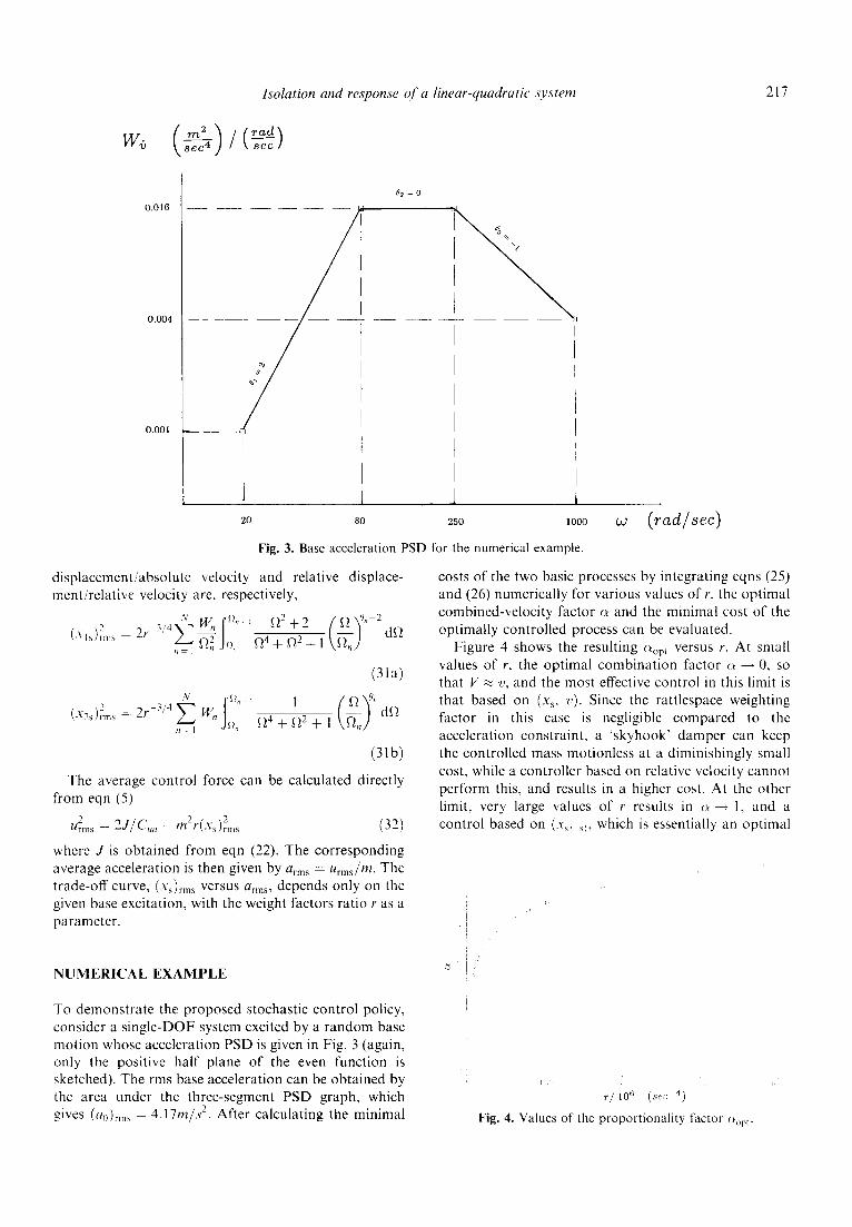
Fig. 3. Base acceleration PSD for the numerical example.

displacement/absolute velocity and relative displace- ment/relative velocity are, respectively,

2 r 3 " 4 ~ " ~ - n / [~2+2

(31a)

(-"2s)~m~ = 2r 3'/4 Z W n a2 d [ ] n = 1 £2. [~4 + + 1

(31b)

The average control force can be calculated directly from eqn (5)

2 2 J / C . . 2 2 " r m s -- - - m r(Xs)rm s (32)

where J is obtained f rom eqn (22). The corresponding average acceleration is then given by arm s : Urms/m. The trade-off curve, (x~)~m~ versus arms, depends only on the given base excitation, with the weight factors ratio r as a parameter.

N U M E R I C A L E X A M P L E

costs o f the two basic processes by integrating eqns (25) and (26) numerically for various values of r, the optimal combined-velocity factor ~ and the minimal cost o f the optimally controlled process can be evaluated.

Figure 4 shows the resulting ~op~ versus r. At small values of r, the optimal combinat ion factor ¢t ~ 0, so that V ~ v, and the most effective control in this limit is that based on (Xs, v). Since the rattlespace weighting factor in this case is negligible compared to the acceleration constraint, a ' skyhook ' damper can keep the controlled mass motionless at a diminishingly small cost, while a controller based on relative velocity cannot perform this, and results in a higher cost. At the other limit, very large values of r results in (~ ~ 1, and a control based on (x s, ~/, which is essentially an optimal

i j

i I :

b ! ,i

To demonstrate the proposed stochastic control policy, consider a s ingle-DOF system excited by a r andom base motion whose acceleration PSD is given in Fig. 3 (again, only the positive half plane o f the even function is sketched). The rms base acceleration can be obtained by the area under the three-segment PSD graph, which gives (a0)rm., 4.17m/s 2. After calculating the minimal

r~ 106 ( sec 4)

Fig. 4. Values of the proportionality factor (~opt.

218 Y. Narkis , C.S. Lyrintz is

~ q

i

/

! ii &

%-

o o o c 8 0 0 12C.0 1~0.0

r/ lO 6 (~ec 4)

Fig. 5. Comparison of minimal costs for the basic controllers J1, J2 and for the combined-state controller Jmi,~.

passive control setup, is superior. For ali intermediate values of r, the approPriate Crop t c a n be found from the graph and used to determine the combined-velocity variable.

The cost of the combined-state controlled process, Jmi~_, is pIotted in Fig. 5 along with the minimal costs of the two basic processes. I t can be seen that the 'break even' point between the basic processes is at r ~ 53 x 106 s -4. Below this value Ji is smaller, so that the 'skyhook' control is more effective, and above this value the optimal passive control yields a lower cost. The cost of the control based on the combined variable vector, (Xs, V), is always lower than those of the basic processes, and at the break-even point it is just half the cost of either process.

The trade-off curves for the three controls are plotted in Fig. 6, for values of 3 x 106 < r < 154 × 106 S -4 , ~t SHOWS the trade-off between the two response para- meters, which had to be minimized subject to the dynamic equations and the given cost function. It can be seen that the optimal 'skyhook' control restricts mainly the acceleration, at the cost off higher displacement. The passive optima1 control is characterized by smaller displacements, but higher accelerations. The curve of the combined-state control exhibits a considerable improvement when compared to the less-alleviated response parameter of each of the basic controllers (e.g. acceleration for the passive isolation), at a slightly higher value of the other response parameter. This resutts in a lower total cost for the combined-state controller, as was shown previously in Fig. 5.

C O N C L U S I O N S

A combined-state variable vector was suggested for use in the optimal control of a linear-quadratic process, excited by stationary random vibrations. The minimal cost and trade-off curve for the optimally controIted

2'

2

oi d i

0.0

(z~, v) s~ghook

k'Zs~ ~s) p~NS~V~

~,~ i ~ / ~ =)

F~g. 6° Trade-off cnrves for the three con~rotlers~

process can be calculated when the input is approx~ mated by a piecewise-tinear PSD in the tog W,~-log_ plane. Numerical results were given for a singleoDOF system which has to be isoiated from a random base motion, described by a three-segment PSD curve. This typical case shows the advantage of the combined-state control over the traditionai passive or ~skyhook ~ controllers in a total process cos~ f-auction and on it5 trade-off curve.

ACKNOWLEDGEMENT

This work was supported in par~ by a gran~ from the San Diego State University Foundation.

REFERENCES

t. Karnopp, D.C., Active damping in road vehicle suspen- sion systems. Vehicle System Design, i2 (1983) 291-316.

2. Hac, A., Suspension optimization of a 2-DOF vehicle model using a stochastic optimal comro? tec1~nique. Journal o f Sound and Vibration, 108 (198D 343-57~

3. Nishimura, H., Yoshida, K & Shimogo, T.. Optimal dynamic vibration absorber for multi-degree-of-Ereedom systems. J S M E International gournai, series 3. 32 (!989) 373-9.

4. Politansky, H. & Pilkey, W.D.. Suboptimal feedback vibration control of a beam with a oroof-rnass actuator. Journal of Guidance, Control and Dynamics. t2 (19891 691 7.

5. Raju, P.K. & Sun, S.K. Modal control of a flexibie beam with multiple sensors and actuators. 12th Biennia[ ASM'E Conference on Mechanical Vibration and Noise. Montreal Canada, Sept. 17-21, 1989.

6. Meirovitch, L. & Kwak, M.K., Control of spacecraft with multi-targeted flexibie antennas. Journal of the Astrona~,~- tical Sciences, 38 (1990) i87-99.

7. Fnkuda, T. & Arakawa, A., Control of a flexibte space manipulator with three degrees of freedom. ]6g,~ inter- national Symposium of Space TechnoIogy and. Science Sapporo, Japan, May 22-27. i988.

Isolation and response of a linear-quadratic system 219

8. Sevin, E. & Pilkey, W.D., Optimum Shock and Vibration Isolation. Shock and Vibration Monograph No. 6, The Shock and Vibration Information Center, Naval Research Center, Washington, DC, 1971.

9. Karnopp, D.C. & Trikha, A.K., Comparative study of optimization techniques for shock and vibration isolation, ASME Journal of Engineering .for Industry, 91 (1969) 1128 32.

10. Stengel, R.F., Stochastic Optimal Control. John Wiley, New York, 1986.

11. Narkis, Y. & Lyrintzis, C.S., Optimal control of linear- quadratic processes using combined state variables. J. Sound and Vibration (submitted for publication).

12, Narkis, Y., Cost function calculation for stationary, linear- quadratic systems with colored noise. 1EEE Transactions on Automatic Control, 37 (1992) 1772 4.