Optimal Model Complexity in Geological

Carbon Sequestration: A Design of

Experiment (DoE) & Response Surface (RS)

Uncertainty Analysis

DE-FE-0009238

Ye Zhang1, Mingkan Zhang1, Peter Lichtner2

1. Dept. of Geology & Geophysics, University of Wyoming, Laramie, Wyoming

2. OFM Research, Inc., Santa Fe, New Mexico

U.S. Department of Energy

National Energy Technology Laboratory

Strategic Center for Coal’s

FY16 Carbon Storage Annual Review Meeting

August 16-18, 2016, Pittsburg, PA

2

Project Objectives

Overall Goals:

1. Support industry’s ability to predict CO2 storage capacity

in geologic formations to within ±30% accuracy;

2. Develop and validate technologies to ensure 99% storage

permanence.

Specific Objectives:

For GCS in environments with permeability (k) heterogeneity:

1. develop lower resolution, cost-effective, and fit-for-purpose models

that can be built with limited data at reduced cost;

2. explore subsurface conditions (offshore Gulf of Mexico) that lead to

gravitationally stable trapping;

A typical CO2 storage reservoir:

• Physically and chemically heterogeneous at multiple scales, e.g., lamina, bedding,

facies, facies assemblage, formation.

• Site characterization data are not sufficient to resolve small-scale reservoir

petrophysical and geochemical variability.

• Reservoir heterogeneity is represented at some “homogenization scale”, e.g.

1. A facies model was used to simulate CO2 storage at Sleipner, ignoring sub-facies

heterogeneity.

2. A formation model was used to evaluate pore pressure from CO2 injection into the Mt Simon

sandstone in Illinois Basin, ignoring heterogeneity within the sandstone.

• What is the conceptual model uncertainty in CO2 modeling?

• Is small-scale heterogeneity important for making large-scale long-term

predictions?

• Can lower resolution models be useful? And, what are their uses?

3

Motivation

We evaluate conceptual models at different resolutions to determine

the condition under which low-resolution models can be used to

evaluate GCS performance metrics.

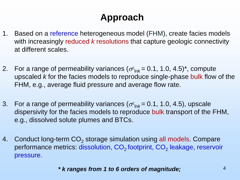
Approach

1. Based on a reference heterogeneous model (FHM), create facies models

with increasingly reduced k resolutions that capture geologic connectivity

at different scales.

2. For a range of permeability variances (s2lnk = 0.1, 1.0, 4.5)*, compute

upscaled k for the facies models to reproduce single-phase bulk flow of the

FHM, e.g., average fluid pressure and average flow rate.

3. For a range of permeability variances (s2lnk = 0.1, 1.0, 4.5), upscale

dispersivity for the facies models to reproduce bulk transport of the FHM,

e.g., dissolved solute plumes and BTCs.

4. Conduct long-term CO2 storage simulation using all models. Compare

performance metrics: dissolution, CO2 footprint, CO2 leakage, reservoir

pressure.

4* k ranges from 1 to 6 orders of magnitude;

5. Develop, test, and verify a Design of Experiment (DoE) and Response

Surface (RS) uncertainty analysis for all models to evaluate:

1. If facies models can capture the “parameter space” of the FHM, i.e., key

parameters that impact the long-term performance metrics.

2. If facies models can capture the “prediction space” of the FHM, i.e.,

uncertainty envelope of each performance metric;

3. Determine an optimal facies resolution for each performance metric.

4. Identify a low resolution model for reservoir analysis in lieu of the FHM.

6. Investigate increasing reservoir depth on storage security: conduct a

global sensitivity analysis to evaluate CO2 storage in GOM sediments.

7. Develop upscaling relations for geochemical parameters of the facies

models. Determine optimal resolutions.

5

Approach

6

Data from the XES facility

http://www.safl.umn.edu/Prof. Chris Paola

0.5 billion cells

XES Prototype experiment (1996)

7

Conceptual Reservoir Models

Lx=5,000 m, Ly=5,000 m, Lz=400 m

Nx=251, Ny=251, Nz=40

FHM 8-unit facies model 3-unit facies model

• A 1-unit formation model, where a single k* is computed, is also created.

s2lnk=4.5

Decreasing resolution, decreasing cost

3.2×106 individual k values 8 individual k* values 3 individual k* values

8

Intrinsic Permeability Upscaling

BC1

BC2

BCm

Symmetry

…

Zhang et al. (2006) WRR; Li et al. (2011) WRR

9

Permeability Upscaling & Verification

Reservoir Fluid Pressure Comparison

,HSM ,ref

1 i,ref

1100%

li i

i

h hMRE

l h

• MRE for predicting the single-phase flow rate is similar to MRE for pressure

prediction. When lnk variance is lower (0.1, 1.0, 4.5), both errors decrease

from those of s2lnk =7.

• For a given s2lnk, P and flow rate prediction accuracy: 1-unit model < 3-unit

model < 8-unit model.

• When s2lnk = 7, optimal resolution is the 3-unit model if we accept ~5% error

in P and flow rate. If we reduce the error threshold, a higher resolution

model (i.e. ,8-unit) is required.

• When s2lnk = 0.1, the 1-unit model is optimal for identical error thresholds;

When s2lnk >>1.0, the 1-unit model is inaccurate: it fails to capture k

connectivity which, under high variance, becomes preferential flow.

• Optimal resolution depends on user-specified error

thresholds and the underlying system variability.

Dispersivity Upscaling & Verification

• For a given variance, accuracy in

transport prediction: 8-unit > 3-unit

> 1-unit model;

• For s2lnk up to 4.5, 8- and 3-unit

models can accurately capture the

plume migration pathway, mass

centroid, and plume dimensions;

Optimal resolution: 3-unit model.

• For s2lnk = 0.1, all models can

accurately capture transport BTC;

Optimal resolution: 1-unit model.

• For s2lnk = 4.5, only the 8-unit

model can capture some aspects

of transport BTC; Optimal

resolution: 8-unit or higher.

• Solute transport is more

sensitive to heterogeneity

resolution. Optimal resolution

depends on the prediction

goal and the underlying

system variability.

Zhang & Zhang (2016) WRR

CO2 Storage Modeling

11

Lx=5,000 m, Ly=5,000 m, Lz=600 m

Nx=251, Ny=251, Nz=60

3.78M grid cells

12

CO2 Modeling with PFLOTRAN

Multicomponent-multiphase-multiphysics non-isothermal reactive flow and

transport simulator (Multilab open source code: LANL, LBNL, ORNL, PNNL);

Massively parallel---based on the PETSc parallel framework; Peta-scale performance

Highly scalable (run on over 265k cores)

Supercritical CO2-H2O Span-Wagner EOS for CO2 density & fugacity coefficient

Mixture density for dissolved CO2-brine (Duan et al., 2008)

Viscosity CO2 (Fenghour et al., 1998)

Pc assumed zero for viscous (injection) and gravity flow (monitoring);

Relative permeability (van Genuchten-Mualem) has no residual trapping;

Finite Volume Discretization Variable switching for changes in fluid phase

Operator splitting for modeling transport and reactions

Structured/Unstructured grids

Object oriented Fortran 2003;

http://www.pflotran.org/

13

Performance Scaling on Yellowstone

Yellowstone is a 1.5-petaflops supercomputer with 72,288 processor cores & 144.6 TB of memory.http://www2.cisl.ucar.edu/resources/yellowstone

A test run (1-unit model; 25 M grid cells) simulating CO2 injection

• Injecting scCO2 for 10~40 years; total simulation time = 2000 years;

• 4 uncertainty factors identically varied for each conceptual model in a 3-

level Box–Behnken design:

geothermal gradient; k of caprock; brine salinity; injection rate*

• The same set of experiments for all models to evaluate their parameter &

prediction space; 300 simulations at 3 reservoir variances (0.1, 1.0, 4.5);

Design of Experiment for CO2 Storage

* Injection duration is varied so the

same amount of CO2 is injected.

A facies model of the

lowest resolution that

can capture the

parameter & prediction

space of the FHM is

considered optimal.

15

Parameter Ranking

Outcome = dissolution storage at 2,000 years

Though not capturing the numerical values of the importance statistics of the

FHM, all facies models have captured the correct parameter ranking regardless of

system lnk variance.

For the given ranges of the parameters varied, the most important parameter

influencing dissolution storage is salinity.

16

Parameter Ranking

Outcome = total leakage of CO2 at 2,000 years

Though not capturing the numerical values of the importance statistics of the

FHM, all facies models have captured the correct parameter ranking regardless of

system lnk variance.

For the given ranges of the parameters varied, the most important parameter

influencing CO2 leakage is caprock permeability.

17

Response Surface Modeling (1-Unit; s2lnk=0.1)

Outcome= dissolution storage

End of

Injection

End of

Monitoring

Ongoing work:

• Create cdf of different

predictions at two time

scales for all models and

for all 3 system variances;

• Uncertainty of all

predictions using all

models will be compared.

18

Case 1: isosurface of dissolved CO2 at 0.004 liquid mole fraction at 2000

years with σ2 = 0.1 (a - d) and σ2 = 4.5 (e -h).

• In the weakly heterogeneous system, convective mixing is simulated by all models.

• In the strongly heterogeneous system (σ2 =4.5), convective mixing is suppressed

by the representation of heterogeneity.

19

CO2 dissolution over time for case 2 (high salinity) and case 1 (low salinity):

σ2 = 0.1 σ2 = 1.0 σ2 = 4.5

Under high salinity, for all variances, heterogeneity resolution is not important because

convective mixing is suppressed: 1-unit model is optimal.

Under low salinity, for all variances, 1-unit model overestimates dissolution by up to

40% due to enhanced convective mixing; 3-unit model is optimal.

20

s2lnk=4.5

t (year)

p(

10

7P

a)

100

101

102

1032.188

2.189

2.19

1unit

FHM

t (year)

p(

107

Pa)

100

101

102

1032.004

2.008

2.012

2.016

1unit

FHM

relative P

error =0.5%

t (year)

p(

107

Pa)

100

101

102

1032.0918

2.0919

2.092

2.0921

2.0922

1unit

FHM

t (year)

p(

107

Pa)

100

101

102

1031.954

1.96

1.966

1.972

1.978 1unit

FHM

[2510, 2510, 205]

[2510, 2510, 445]

[2510, 2510, 305]

[2510, 2510, 395]

FHM v. 1-Unit Model Pressure Comparison

Caprock

21

Offshore Storage (Gulf of Mexico)

• Offshore environments:

(1) low T and high P; (2)

infrastructure (boreholes

and pipelines) from oil

gas development, Close

et al., [2008], Han et al.,

[2009], Li et al. [2010],

among others.

• Wells have been drilled to

10 km depth, and both

saline aquifer storage

and CO2-EOR is

possible.

• Based on GOM sediment and geothermal data, a global sensitivity analysis: (1)

identify key parameters that impact CO2 storage & leakage; (2) evaluate conditions

for gravity stable storage. 1000 simulations carried out.

22

Uncertain Input parameters* Min. Max. Base

case

Distribution

Reservoir

Property

Sediment thickness (km) 0.005 0.9 500 Uniform

Mean permeability (D) 0.001 8 1.0 Log uniform

Permeability anisotropy factor 0.01 0.5 0.1 Uniform

Permeability variance 0.0 5.0 0/1.0 Uniform

Horizontal integral scale (km) 0.5 5.0 1.0 Uniform

Mean porosity 0.1 0.42 0.2 Correlated to

perm

Physical

Parameter

Water depth (km) 0.1 4.4 2.5 Uniform

CO2 injection rate (kg/s) 0.002 2.0 0.3 Correlated to

depth

Seafloor temperature (ºC) 1 20 2 Correlated to

depth

Geothermal gradient (ºC/km) 5 50 20 Correlated to

depth

* Based on sediment data collected from 4 GOM sites; temperature and geothermal gradients are from

literature. See detail in Dai, Zhang, Stauffer, et al. (2016) Identification of Gravitational Trapping

Processes of CO2 Sequestration in Offshore Marine Sediments, poster presentation, this meeting.

23

See detail in Dai, Zhang, Stauffer, et. al (2016) Identification of Gravitational Trapping Processes of

CO2 Sequestration in Offshore Marine Sediments, poster presentation, this meeting.

Summary of Progress

• Created high-resolution FHM from an Experimental Stratigraphy; scale it to

increasing lnk variances (0.1, 1.0, 4.5);

• For each variance, created 3 facies models to with reduced k resolutions;

• Multiscale, multi-variance flow & transport upscaling and verification;

• Multiscale, multi-variance CO2 storage modeling using PFLOTRAN:

• Under increasing reservoir variability, conduct DoE and RS modeling;

evaluate optimal resolution for predicting each performance metric.

(1) scaling on petascale Yellowstone supercomputer at NCAR-Wyoming Supercomputing Center.

(2) CO2 simulations and uncertainty analysis have used ~12 million core hours.

• Investigated increasing depth on storage security. Completed a suite of

uncertainty analysis using reservoir parameters from the Gulf of Mexico.

• Developed improved geochemical relations for CO2-fluid-rock reactions.

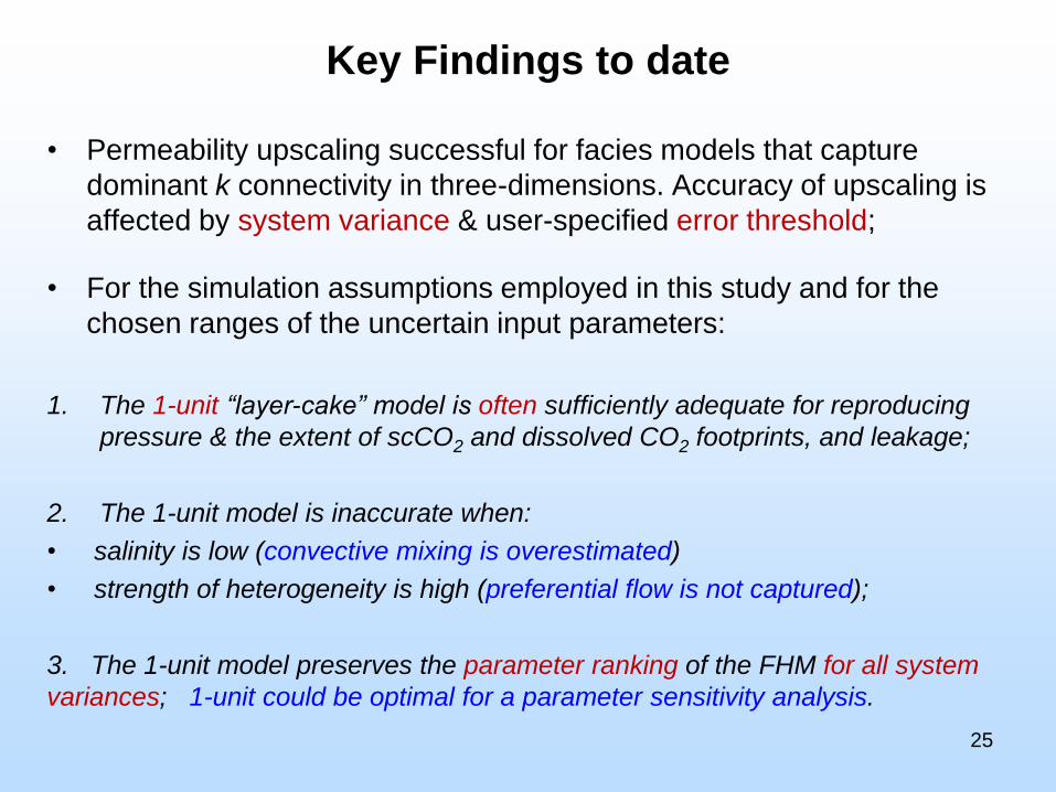
Key Findings to date

• Permeability upscaling successful for facies models that capture

dominant k connectivity in three-dimensions. Accuracy of upscaling is

affected by system variance & user-specified error threshold;

• For the simulation assumptions employed in this study and for the

chosen ranges of the uncertain input parameters:

1. The 1-unit “layer-cake” model is often sufficiently adequate for reproducing

pressure & the extent of scCO2 and dissolved CO2 footprints, and leakage;

2. The 1-unit model is inaccurate when:

• salinity is low (convective mixing is overestimated)

• strength of heterogeneity is high (preferential flow is not captured);

3. The 1-unit model preserves the parameter ranking of the FHM for all system

variances; 1-unit could be optimal for a parameter sensitivity analysis.

25

Key Findings to date

4. Dissolution, leakage, footprint, and pressure can be captured by the 3-unit

model for all system variances; An overall optimal model.

5. Brine salinity is the single most influential factor impacting dissolution while

caprock is the single most influential factor impacting leakage. This finding is

independent of the conceptual models and the system variability tested;

• History matching using fluid pressure & plume sizes alone cannot lead to

the unique estimation of k, as under many conditions, different k

parameterizations (8-, 3-, 1-unit) can match these performance metrics

equally well. Detailed multiphase saturation and CO2 breakthrough data

are likely needed.

26

27

Key Findings to date

Sensitivity analysis with the Gulf of Mexico data:

1. When lnk variance is high, gravitational trapping can be achieved

at a water depth of 1.2 km, extending previously identified self-

sealing conditions requiring water depth > 2.7 km.

2. Strong permeability/porosity heterogeneity can enhance

gravitational trapping.

Ongoing Research

Our simulation studies have limitations;

Relative permeability upscaling under different capillary, viscosity,

versus gravity regimes.

Upscaling of geochemical parameters for the ‘facies’ models;

Develop new reservoir inversion techniques to identify and

parameterize facies models without upscaling (Jiao & Zhang, 2016).

28

29

Bibliography

• Mingkan Zhang, Ye Zhang (2015) Multiscale Dispersivity Upscaling for Three-Dimensional

Hierarchical Porous Media, Water Resources Research, 51, doi:10.1002/2014WR016202.

• Jianying Jiao, Ye Zhang (2016) Direct Method of Hydraulic Conductivity Structure

Identification for Subsurface Transport Modeling, Journal of Hydrologic Engineering,

10.1061/(ASCE)HE.1943-5584.0001410, 04016033.

• Lichtner, Peter (2016) Kinetic Rate Laws Invariant to Scaling the Mineral Formula Unit,

American Journal of Science, in press.

• Mingkan Zhang, Ye Zhang, Peter Litchtner (2016) Uncertainty analysis in modeling CO2

dissolution in three-dimensional heterogeneous aquifers: effect of multiple conceptual models

and explicit fluid flow coupling, International Journal of Greenhouse Gas Control, in

submission.

• Zhenxue Dai, Ye Zhang, Phil Stauffer, Mingkan Zhang, et al. (2016) Identification of

gravitational trapping processes of CO2 sequestration in offshore marine sediments, Natural

Geoscience, in prep.

Extra Slides

30

31

Presentation Outline

– Project Objectives

– Study Approach

– Progress to Date on Key Technical Issues

– Project Wrap-Up

Plans for Remaining Technical Issues

32

• Complete the geochemical upscaling study to evaluate if

HSMs can capture mineral storage when the system

contains significant amount of (homogeneous versus

heterogeneously distributed) reactive minerals.

• Complete the DoE and RS analysis for all static models

with mineral reactions to compare their parameter

sensitivity & prediction uncertainty.

• Evaluate the uncertainty in the EOS, which is relevant for

identifying suitable conditions for gravity-stable injection

in both onshore and offshore settings.

33

Heterogeneity, Physiochemical Coupling,

& Feedback

Base case: No upscaling of geochemical parameters (assume the same

bulk mineralogy and reactive mineral parameters):

• How does the resolution of physical heterogeneity affects flow paths and

therefore reaction sites and rates and ultimately mineral storage?

• How important is the change in porosity due to the reactions? If

important, then feedback between flow and rxn must be accounted for.

• Common assumptions (e.g., Xu et al., 2003, 2004, 2007; Liu et al.,

2011; Zhu et al., 2013), neglecting the effect of physical heterogeneity,

physiochemical coupling, and (often) porosity-permeability changes and

their feedback with flow.

Upscaling mineral specific surface areas

1) Issues linking grain size to FHM's permeability distribution:

• Different published sources reported distinct grain size-permeability relationships

for sandstones.

• If any given grain size-permeability relation is used to estimate reactive surface

area, the reactive surface areas for different minerals will be the same, which is not

consistent with detailed laboratory measurements reported in the literature.

2) Issues using surface roughness to distinguish different minerals:

• The calculated reactive surface area using surface roughness is several orders of

magnitude different from the experiment data from the literature.

3) Issues using an empirical formula directly linking grain size to reactive

surface area:

Grain size is no longer a constant value compared to experiment data from the

literature. Therefore, we have to measure grain size for every mineral.

4) Issues using an empirical formula directly linking reactive surface area to lnk:

High uncertainty (ranging form positive, zero, to negative) exists in their correlation.

34

35

Parallel Simulation for k Upscaling

Test model (0.4M):

Serial time (calling an optimized IMSL on BigRed at IU): 1 hour

Parallel time (H2oc.gg.uwyo.edu): 37 sec (64 processors)

36

37

Code Comparison with TOUTHREACT

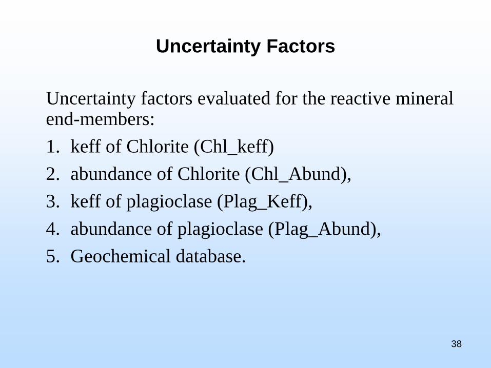
Uncertainty Factors

38

Uncertainty factors evaluated for the reactive mineral end-members:

1. keff of Chlorite (Chl_keff)

2. abundance of Chlorite (Chl_Abund),

3. keff of plagioclase (Plag_Keff),

4. abundance of plagioclase (Plag_Abund),

5. Geochemical database.

Uncertainty Factors

39

Uncertainty factors evaluated for the fast-reactingmineral end-members:

1. keff of Chlorite (Chl_keff)

2. abundance of Chlorite (Chl_Abund),

3. keff of plagioclase (Plag_Keff),

4. abundance of plagioclase (Plag_Abund),

5. Database.

40

Chl_Keff Chl_Abund Plag_Keff Plag_Abund Database

10 0 -1 0 L2

2-1 1 -1 -1 L2

30 0 0 0 L2

40 1 0 0 L1

51 1 -1 1 L2

60 -1 -1 1 L1

71 -1 0 0 L1

80 0 0 -1 L2

9-1 0 -1 -1 L1

101 -1 -1 -1 L2

11-1 -1 1 1 L1

121 -1 1 1 L2

13-1 1 -1 1 L1

141 0 1 -1 L1

15-1 -1 0 1 L2

16-1 0 0 0 L1

17-1 1 1 -1 L1

181 0 0 1 L1

191 1 1 -1 L2

200 1 1 1 L1

21-1 1 1 1 L2

221 1 -1 -1 L1

23-1 -1 -1 0 L2

24-1 -1 1 -1 L2

250 -1 0 -1 L1

260 0 1 0 L2

Changes in Volume Fraction: Chlorite after 2000 years

41

Changes Volume Fraction:

Siderite after 2000 years

42

Changes Volume Fraction:

Magnesite after 2000 years

43

Changes Volume Fraction:

without Chlorite after 2000 years

44

45

Chl_Keff Chl_Abund Plag_Keff Plag_Abund Database

10 0 -1 0 L2

2-1 1 -1 -1 L2

30 0 0 0 L2

40 1 0 0 L1

51 1 -1 1 L2

60 -1 -1 1 L1

71 -1 0 0 L1

80 0 0 -1 L2

9-1 0 -1 -1 L1

101 -1 -1 -1 L2

11-1 -1 1 1 L1

121 -1 1 1 L2

13-1 1 -1 1 L1

141 0 1 -1 L1

15-1 -1 0 1 L2

16-1 0 0 0 L1

17-1 1 1 -1 L1

181 0 0 1 L1

191 1 1 -1 L2

200 1 1 1 L1

21-1 1 1 1 L2

221 1 -1 -1 L1

23-1 -1 -1 0 L2

24-1 -1 1 -1 L2

250 -1 0 -1 L1

260 0 1 0 L2

Changes in Volume Fraction: Chlorite after 2000 years

46

47

48

FHM v. 1-Unit Model

Dissolved CO2 at the end of monitoring (inj rate= 0.05 Mt/yr):

5km

5km

400 m

Under both low and high variances, for the given combination of dynamic

parameters, the 1-unit model can capture plume footprint and fluid pressure

distribution of the FHM well. For these performance metrics, 1-unit model is

sufficient, even though the 8-unit and 3-unit models yield more accurate

predictions (not shown);

(An identical set of DoE dynamic parameters)

49

FHM v. HSMs (Dissolved CO2 plume )

Under high reservoir lnk variances, for the given combination of dynamic

parameters, the 1-unit model can capture scCO2 plume footprint and fluid

pressure distribution of the FHM well. For these performance metrics, 1-unit

model is sufficient, even though the 8-unit and 3-unit models yield more

accurate predictions (not shown);

(An identical set of DoE dynamic parameters)

Dissolved CO2 at the end of monitoring (inj rate= 0.063 Mt/yr):

5km

5km

400 m

50

FHM v. 1-Unit Model (Dissolved CO2 Plume)

Dissolved CO2 at the end of monitoring

(An identical set of DoE dynamic parameters)

Low salinity (0 Molal) &

Low injection rate (0.252 Mt/yr for 10 yr)

High salinity (4.0 Molal) &

High injection rate (0.063 Mt/yr for 40 yr)

Medium caprock permeability 1E-17.5 m2 and medium temperature gradient -0.0375oc/m

51

FHM v. 1-Unit Model (scCO2 Plume) (An identical set of DoE dynamic parameters)

scCO2 at the end of monitoring

Medium caprock permeability 1E-17.5 m2 and medium temperature gradient -0.0375oc/m

Low salinity (0 Molal) &

Low injection rate (0.252 Mt/yr for 10 yr)

High salinity (4.0 Molal) &

High injection rate (0.063 Mt/yr for 40 yr)

Design of Experiment (1-Unit; s2lnk=0.1)

52

Pattern T_Gradient Brin_Salinity K_Cap Inj_rate DC_EOI DC_EOM

−−00 -1 -1 0 0 6.00E+06 4.73E+07

−+00 -1 1 0 0 3.41E+06 1.13E+07

+−00 1 -1 0 0 5.98E+06 4.75E+07

++00 1 1 0 0 2.56E+06 1.89E+07

00−− 0 0 -1 -1 5.64E+06 2.04E+07

00−+ 0 0 -1 1 5.13E+06 2.14E+07

00+− 0 0 1 -1 3.94E+06 1.72E+07

00++ 0 0 1 1 4.09E+06 1.83E+07

−00− -1 0 0 -1 4.80E+06 1.89E+07

−00+ -1 0 0 1 4.34E+06 2.00E+07

+00− 1 0 0 -1 4.79E+06 1.88E+07

+00+ 1 0 0 1 4.31E+06 1.98E+07

0−−0 0 -1 -1 0 7.28E+06 4.85E+07

0−+0 0 -1 1 0 5.50E+06 4.66E+07

0+−0 0 1 -1 0 4.00E+06 1.27E+07

0++0 0 1 1 0 2.92E+06 9.92E+06

−0−0 -1 0 -1 0 5.28E+06 2.10E+07

−0+0 -1 0 1 0 3.91E+06 1.77E+07

+0−0 1 0 -1 0 5.27E+06 2.08E+07

+0+0 1 0 1 0 3.89E+06 1.75E+07

0−0− 0 -1 0 -1 6.63E+06 4.86E+07

0−0+ 0 -1 0 1 5.92E+06 4.71E+07

0+0− 0 1 0 -1 3.62E+06 1.10E+07

0+0+ 0 1 0 1 3.33E+06 1.18E+07

0000 0 0 0 0 4.43E+06 1.92E+07

Environmental/engineering factors Dissolved CO2 at 2 time scales

• The DoE runs for a given

static model use the same

injector, injecting the same

amount of CO2, and

assuming the same BC.

• Identical DoE is used for all

static models.

• Total simulations = 25 (DoE)

x 4 (models) x 3 (lnk

variances) =300

53

Parameter Ranking (1-Unit; s2lnk=0.1)

End of

Injection

End of

Monitoring

Outcome:

dissolved CO2

CO2 Simulation: Mineral Trapping

• Reactive minerals in sandstone such as chlorite and plagioclase can

provide cations such as Mg2+, Fe2+, and Ca2+, which are essential

chemical components for forming carbonate precipitates during GCS

(Xu et al., 2012).

• The reactions between cations and CO2 forms carbonate minerals

(e.g., calcite, siderite, magnesite, and ankerite) to trap CO2 as

precipitates.

• When modeling mineral storage, uncertainty exists in (1) reactive

mineral volume fractions; (2) reactive surface areas; (3) kinetic rate

parameters; (4) thermodynamic database.

• When we have multiple static models, uncertainty also exists in

upscaling geochemical reaction parameters (e.g., mineral volume

fractions, reactive surface areas).54

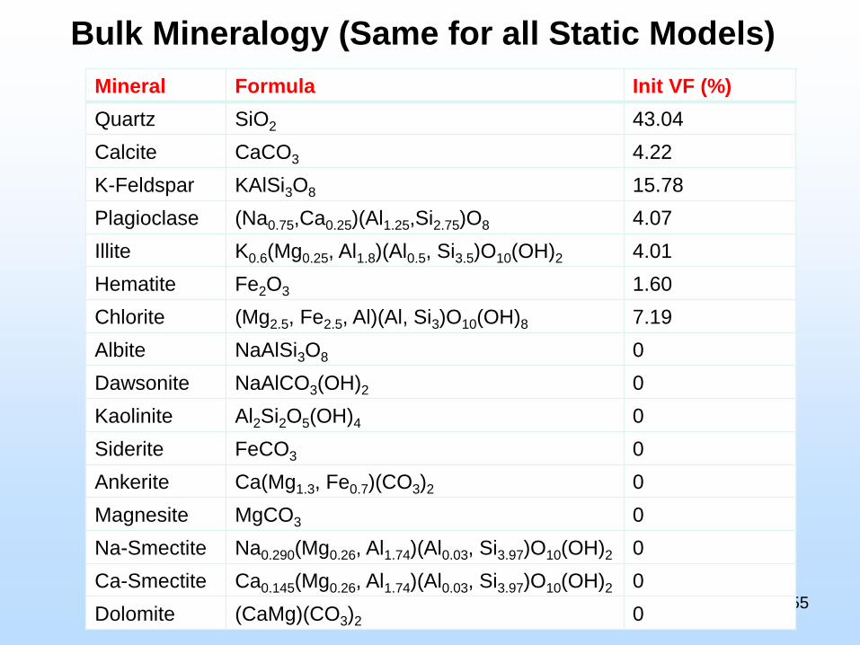
Bulk Mineralogy (Same for all Static Models)

55

Mineral Formula Init VF (%)

Quartz SiO2 43.04

Calcite CaCO3 4.22

K-Feldspar KAlSi3O8 15.78

Plagioclase (Na0.75,Ca0.25)(Al1.25,Si2.75)O8 4.07

Illite K0.6(Mg0.25, Al1.8)(Al0.5, Si3.5)O10(OH)2 4.01

Hematite Fe2O3 1.60

Chlorite (Mg2.5, Fe2.5, Al)(Al, Si3)O10(OH)8 7.19

Albite NaAlSi3O8 0

Dawsonite NaAlCO3(OH)2 0

Kaolinite Al2Si2O5(OH)4 0

Siderite FeCO3 0

Ankerite Ca(Mg1.3, Fe0.7)(CO3)2 0

Magnesite MgCO3 0

Na-Smectite Na0.290(Mg0.26, Al1.74)(Al0.03, Si3.97)O10(OH)2 0

Ca-Smectite Ca0.145(Mg0.26, Al1.74)(Al0.03, Si3.97)O10(OH)2 0

Dolomite (CaMg)(CO3)2 0

56

Mineral Mass Balance (1-unit model)

CO2 is injected at 10 kg/s for 10 years or 3.1536*109 kg

After 40,000 years,

around 10% of the

injected CO2 has

been transformed

to carbonate

minerals

Onshore simulations using the

Span-Wagner EOS suggest that a

very low geothermal gradient is

needed to develop conditions

suitable for gravity-stable injection.

Such cool conditions may exist in

parts of the continental US. We’re

collecting data from these locations

to obtain precise in-situ reservoir T

and P data before repeating the

simulations.

57

Deep Storage: Onshore

Bachu & Stewart (2002)

MIT (2006)

58

Deep Storage: Off-shore

Personal

communication,

Phil Stauffer, Feb

(2015); Also, Levine

et al. (2013)

When gravity stable, caprock for the reservoir is not needed