optimal patent policy for pharmaceutical industry
TRANSCRIPT

Olena IzhakTanja SaxellTuomas Takalo
Optimal Patent Policy for Pharmaceutical Industry
VATT INSTITUTE FOR ECONOMIC RESEARCH
VATT Working Papers 131

VATT WORKING PAPERS
131
Optimal Patent Policy for Pharmaceutical Industry
Olena Izhak Tanja Saxell
Tuomas Takalo
Valtion taloudellinen tutkimuskeskus VATT Institute for Economic Research
Helsinki 2020
Olena Izhak, Düsseldorf Institute for Competition Economics, [email protected]
Tanja Saxell, VATT Instute for Economic Research, [email protected]
Tuomas Takalo, Bank of Finland and VATT, [email protected]
We thank Vanessa Behrens, Vincenzo Denicolò, Alberto Galasso, Matthew Grennan, Dietmar Harhoff, Jussi Heikkilä, Ari Hyytinen, William Kerr, Matthew Mitchell, Petra Moser, Benjamin Roin, Mark Schankerman, Carlos Serrano, Morten Sæthre, Ashley Swanson, Robert Town, Janne Tukiainen, Hannes Ullrich, Rosemarie Ziedonis, and audiences of numerous seminars and conferences for useful comments and discussions. We gratefully appreciate the hospitality of the Economics Departments at Boston and Stanford Universities, and Health Care Management Department of Wharton School where parts of this research has been conducted. We also gratefully acknowledge funding from Yrjö Jahnsson Foundation.
ISBN 978-952-274-253-7 (PDF) ISSN 1798-0291 (PDF) URN:ISBN:978-952-274-253-7 Valtion taloudellinen tutkimuskeskus VATT Institute for Economic Research Arkadiankatu 7, 00100 Helsinki, Finland Helsinki, May 2020

Optimal Patent Policy for Pharmaceutical Industry∗
Olena Izhak
Düsseldorf Institute for
Competition Economics
Tanja Saxell
VATT
Tuomas Takalo
Bank of Finland and VATT
May 10, 2020
Abstract
We show how characterizing optimal patent policy for the pharmaceutical industry only
requires information about generic producers’ responses to changes in the effective duration and
scope of new drug patents. To estimate these responses, we use data on Paragraph IV patent
challenges, and two quasi-experimental approaches: one based on changes in patent laws and
another on the allocation of patent applications to examiners. We find that extending effective
patent duration increases generic entry via Paragraph IV patent challenges whereas broadening
protection reduces it. Our results imply that pharmaceutical patents should be made shorter
but broader.
Keywords: Patent policy, pharmaceuticals, generic entry, innovation, imitation
∗We thank Vanessa Behrens, Vincenzo Denicolò, Alberto Galasso, Matthew Grennan, Dietmar Harhoff, JussiHeikkilä, Ari Hyytinen, William Kerr, Matthew Mitchell, Petra Moser, Benjamin Roin, Mark Schankerman, CarlosSerrano, Morten Sæthre, Ashley Swanson, Robert Town, Janne Tukiainen, Hannes Ullrich, Rosemarie Ziedonis, andaudiences of numerous seminars and conferences for useful comments and discussions. We gratefully appreciate thehospitality of the Economics Departments at Boston and Stanford Universities, and Health Care Management De-partment of Wharton School where parts of this research has been conducted. We also gratefully acknowledge fundingfrom Yrjö Jahnsson Foundation. Contacts: [email protected], [email protected], [email protected].
1

1 Introduction
Patent policy aims at stimulating innovation by providing exclusive rights to innovators at the cost
of reduced competition. This tradeoff between competition and innovation incentives is at the core of
the mature theoretical literature on the optimal design of patent length and scope, dating back to the
seminal works by Nordhaus (1969) and (1972). Empirical studies such as Sakakibara and Branstetter
(2001), Moser (2005), Quian (2007), and Lerner (2009)) provide estimates of the effects of patent
policy reforms on innovation.1 However, these empirical results are not enough to guide the optimal
design of patent length and scope. We combine theory and two-quasi experimental approaches to
characterize optimal patent policy for the US pharmaceutical industry. Our results indicate that
the terms of pharmaceutical patents should probably be shorter and their scope broader. The key
mechanism behind our conclusion is the positive effect of longer patent duration on early generic
entry: we find that one year increase in effective patent length increases generic entry before the
expiration of new drug patents by roughly five percentage points. These results support the theory of
costly imitation pioneered by Gallini (1992), which points to the optimality of broad but short-lived
patents because long-lasting patents encourage to invent around those patents.
The US pharmaceutical industry provides a well-defined setting to assess the theory of costly
imitation: The Drug Price Competition and Patent Term Restoration Act of 1984 (aka the "Hatch-
Waxman" Act) introduced generic drug applications with Paragraph IV (PIV) certifications. In
such a drug application a generic firm certifies noninfringement or invalidity of a new drug patent,
allowing the FDA to approve the application before the expiration of that patent. Hemphill and
Sampat (2011a) and Branstetter et al. (2016) document a substantial increase in such PIV patent
challenges during this millennium.
Our theoretical model shows how characterizing optimal pharmaceutical patent policy only
requires information about generic firms’ entry responses to changes in the effective length and
scope of new drug patents. We estimate the impact of effective patent length on the probability of
PIV entry (that is, a successful PIV patent challenge by a generic entrant). We exploit two patent
law reforms inducing quasi-experimental variation in the effective terms of patents depending on
their prosecution time at the U.S. Patent and Trademark Office (USPTO): First, the Agreement on1Denicolò (1996) and Belleflamme and Peitz (2015, Chapter 19) synthesize the theoretical literature and Boldrin
and Levine (2013), Moser (2013), and Budish et al. (2016) survey the empirical evidence.
1
Trade-Related Aspects of Intellectual Property (TRIPS) of 1994 changed the statutory patent term
from 17 years from the grant date to 20 years from the first filing date. TRIPS also introduced patent
term adjustments (PTAs) to compensate for some delays in patent prosecution, but we document
that those USPTO PTAs were initially insignificant. Second, the American Inventors Protection
Act (AIPA) of 1999 expanded PTAs to compensate for long delays in patent prosecution. We show
how the two reforms affected the effective terms of patents with grant lags exceeding three years,
whereas the effective terms of patents with shorter grant lags were hardly changed.
Using difference-in-differences (DiD) regressions, we find that TRIPS decreased the effective
terms of patents prosecuted at least three years by 17 percent, compared to other patents. This
shorter effective patent length reduced the rate of PIV entry around 8–10 percentage points. In
contrast, AIPA increased the effective terms of patents with the long prosecution lags by 10 percent,
which in turn increased the rate of PIV entry by seven percentage points. These results, together
with supporting evidence from ordinary least squares (OLS) regressions, indicate that longer patent
duration increases PIV entry.
Using multiple measures of patent scope and OLS regressions, we also provide evidence that
broadening patent scope reduces PIV entry. To address the endogeneity of patent scope, we develop
instrumental variables (IV) for some of our scope measures by exploiting differences in the propensity
of some patent examiners to grant broader or more claims. The evidence from our IV regressions
– though not conclusive given the lack of fully randomized examiner assignment (see Righi and
Simcoe, 2019) – implies that extending the scope of patent claims decreases the probability of PIV
entry by about two percentage points.
Our theoretical model yields two formulas characterizing optimal patent policy. These formulas
require as key inputs an estimate of the elasticity of PIV entry with respect to effective patent length
or patent scope. Based on the DiD and IV estimates, we extrapolate the elasticity of PIV entry
with respect to effective length and scope to be around three and −1, respectively. Using these
elasticity estimates in our formulas allows us to predict the effects of changes in patent length and
scope on innovation and welfare. The results point to the optimality of shorter patent length, which
should be compensated by broadening the scope of protection. This conclusion is at odds with
some policies of balancing competition and innovation incentives in the pharmaceutical industry.
For example, the Drug Price Competition and Patent Term Restoration Act – as its name suggests
2

– simultaneously lengthened pharmaceutical patent terms and narrowed their scope by introducing
the FDA patent term extension and PIV patent challenge mechanisms.
Our model builds on the theory of costly imitation developed by Gallini (2002) and later ex-
panded by, e.g., Takalo (1998), Wright (1999), and Maurer and Scotchmer (2002). Our empirical
results concerning patent length are consistent with the findings in Lerner (2009) and Giorcelli and
Moser (2019) showing little effects of longer duration of intellectual property rights on innovation
and creative work. To identify the effects of patent length, we build on the studies on the effects
of TRIPS (e.g., Abrams, 2009; Kyle and McGahan, 2012) and of commercialization lags (Budish
et al., 2015) on innovation in the pharmaceutical industry. To identify the effects of patent scope, we
draw on Kuhn and Thompson (2019), Sampat and Williams (2019) and Farre-Mensa et al. (2020)
who develop similar examiner-leniency IVs. Methodologically, our approach is also close to Deni-
colò (2007) and Budish et al. (2016) who emphasize the estimation of innovation elasticities for the
design of optimal patent policy. We complement these papers by estimating the effects of changes
in patent length and scope on generic entry. Moreover, by using these estimates in our theoretical
formulas, we can characterize optimal patent policy without using data on innovating firms.
A limitation of our study is that we abstract away from the issues related to the effects of patents
on cumulative innovation (e.g., Galasso and Schankerman, 2015; Sampat and Williams, 2019).
2 Optimal Pharmaceutical Patent Length and Scope: Theory
2.1 The Model
We consider a pharmaceutical drug market where two firms, an originator (brand) drug manufac-
turer (firm B) and a generic drug manufacturer (firm G), interact. The originator firm can invest
in developing a new drug, automatically protected by a patent. The generic firm can invest in
challenging the new drug patent.2 We allow for no ex ante licensing.3
2The assumption of only one potential generic entrant is made for simplicity. However, the Drug Price Competitionand Patent Term Restoration Act also stipulates the first successful PIV entrant at minimum a 180-day exclusivityperiod during which no further generic firms are allowed to enter. Allowing free entry to invent around patents wouldnot qualitatively change the results (see, e.g., Gallini, 1992 and Wright, 1999).
3Optimal policy depends on the feasibility of ex ante licensing (see, e.g., Maurer and Scotchmer, 2002). We viewour assumption as reflecting the pharmaceutical industry practice: Our data, as also the findings, e.g., in Hemphilland Sampat (2011a) and Branstetter et al. (2016), show that PIV challenges occur frequently, indicating a failurein the market for ex ante licenses. There is also little evidence of generic entry based on licensing prior to PIVchallenges.
3

Time t ∈ [0,∞) is continuous but, for brevity, we assume that the firms act sequentially at
t = 0 by directly choosing the success probabilities of their investments pf ∈ [0, 1], f = B,G.
(Alternatively, we may think that the firms choose an investment project from a collection of projects
indexed by pf .) The success Yf : {0, 1} → {0, 1} of the firm f ’s investment thus has a Bernoulli
distribution with parameter pf . The associated investment cost functions Cf : [0, 1] → [0,∞),
f = B,G, are twice continuously differentiable with the standard properties ∂Cf/∂pf > 0 and
∂2Cf/∂p2i > 0 for pf > 0, and Cf (0) = ∂Cf (0)/∂pf = 0. The cost functions are sufficiently convex
to satisfy second-order conditions.
We consider two patent policy variables, length (term) T ∈ [0,∞) and scope (breadth) b ∈ [0,∞).
(To simplify the proofs, we allow b and T to only take arbitrarily large but finite values.) As is
common in the theoretical literature (see Budish et al., 2015, for an exception), we assume that a
marketing authorization and a patent are granted to a new drug simultaneously upon the investment
success realization yB = 1 at t = 0, from which patent length is counted. Hence, T reflects effective
new drug patent length. Following Gallini (1992), we assume that the cost of challenging a valid
new drug patent is increasing in b, i.e., ∂CG(pG, b)/∂b > 0. (Maurer and Scotchmer, 2002 argue
for this way of modeling patent scope.) In our context, this assumption means that a broader new
drug patent makes generic entry prior to the patent expiration more difficult. If a patent that has
not been successfully challenged expires at some time t = T , b = 0 for t ≥ T and generic entry will
become costless, CG(pG, 0) = 0. (This assumption can be relaxed in so far entry is cheaper after
the patent expiration.)
After the realizations yf ∈ {0, 1} of Yf , f = B,G, the firms compete in the market. The net
cash flow from selling a drug is given by π̃N ∈ [0,∞), in which subscript N ∈ {0, 1, 2} denotes the
number of competing drugs in the market. The drug market will exist only if yB = 1; otherwise
N = 0 and π̃0 = 0. Conditional on yB = 1, our assumptions imply that N = 1 only if t < T
and yG = 0; otherwise N = 2. For simplicity, we allow no perfect collusion and, hence, π̃1 > 2π̃2.
(The assumption of equal net cash flows in the case of a duopoly can be relaxed at the cost of
complicating the notation.)
Reminiscent of the results in Wright (1999), the shape of the patent challenging cost function
turns out to be crucial for the characterization of the optimal patent policy. We introduce the
4

following definitions to characterize the shape of CG(pG, b) :
εp := pG∂2CG/∂p
2G
∂CG/∂pG, (1)
and
εb := pG∂2CG/∂b∂pG∂CG/∂b
. (2)
In words, εp is the elasticity of the marginal cost of patent challenging, providing us with a measure
of the convexity of the generic firm’s cost function. To avoid the need to check out additional
corners, we assume that εp > 0 for all pG. (The additional restrictions here are mild, since our other
assumptions imply that εp > 0 at least for pG ∈ (0, 1).) In turn, εb is the elasticity of the impact of
patent scope on patent challenging costs. Since ∂CG/∂b > 0, the sign of εb is given by the sign of
∂2CG/∂pG∂b. We proceed under the assumption that ∂2CG/∂b∂pG > 0, i.e.,
Assumption 1. εb > 0.
According to Assumption 1, the effect of patent scope on patent challenging costs is the stronger
the easier is patent challenging. Besides shortening the analysis considerably, making this simpli-
fication has four justifications: First, as shown in Appendix A.1 where we we relax Assumption 1,
effects of patent scope in the case εb ≤ 0 are counterintuitive. For example, if εb < 0, an increase
in patent scope making patent challenging more expensive has a positive impact on the probability
of a successful patent challenge. Such effects can be viewed as being in conflict with the definition
of patent scope. Second, our results concerning patent length are do not depend on Assumption 1
(see Appendix A.1). Third, our empirical results of the negative effect of broader patent scope on
PIV entry provide support for Assumption 1. Fourth, this assumption is often implicitly done in
the previous literature modelling imitation costs as a function of patent scope.
We consider the following two-stage game: In the first stage the originator firm first chooses its
success probability pB(b, T ) ∈ [0, 1]. In the second stage, after observing YB = yb, the generic firm
chooses pG(yB, b, T ) ∈ [0, 1]. The outcome yG ∈ {0, 1} of that investment is realized. The firms
collect their payoffs depending on the realizations of Yf , f = B,G, and patent length T . Denote
the firm f ’s expected profit by Πf , f = B,G. A subgame perfect equilibrium of this game is a pair
(p∗B, p∗G(yB(pB))) such that for all yB(pB) ∈ {0, 1}, p∗G(yB(pB)) = arg maxpG∈[0,1] ΠG(pG, yB(pB))
5

and p∗B = arg maxpB∈[0,1] ΠB(pB, p∗G(yB(pB))).
2.2 Equilibrium Incentives for New Drug Development and Patent Challenging
Consider the second stage of the game after the realization of YB. Clearly, if yB(pB) = 0, the market
for the new drug fails to arise, and p∗G = 0. In what follows, we therefore focus on determining
the part of the equilibrium where the drug market exists, (p∗B, p∗G(yB(pB) = 1)), and suppress the
argument yB(pB) for brevity.
Given yB(pB) = 1, the generic firm’s problem can be written as
maxpG∈[0,1]
ΠG = pG
∞∫0
e−rtπ̃2dt+ (1− pG)
∞∫T
e−rtπ̃2dt− CG(pG, b), (3)
in which r ∈ [0,∞) denotes the firms’ common discount rate. The first integral on the right-
hand side of equation (3) captures the generic firm’s profits if, with probability pG, it successfully
challenges the new drug patent. The second integral captures the profits if, with probability 1−pG,
the challenge fails and the generic entry is postponed until the patent expiration. The last term
captures the costs of patent challenging.
Using the definition π2 := π̃2/r yields the first-order condition for the problem (3) as
(1− e−rT
)π2 −
∂CG(p∗G, b)
∂pG= 0. (4)
The solution to equation (4) implicitly determines the unique p∗G(b, T ) conditional on yB(pB) = 1.
In the first stage the originator firm chooses pB. The private value of an approved new drug to
the originator firm is given by
V P (T, p∗G(b, T )) =
T∫0
e−rt [(1− p∗G (b, T )) π̃1 + p∗G (b, T ) π̃2] dt+
∞∫T
e−rtπ̃2dt, (5)
in which p∗G (b, T ) is determined by equation (4). The first term on the right-hand side of equation
(5) depicts the originator firm’s profits when its new drug patent is in force. The originator firm
will be in a monopoly position if the generic firm’s patent challenge fails (the first term in the
square brackets) but will encounter generic competition if the patent challenge succeeds (the second
6

term in the square-brackets). The second term expresses the originator firm’s profits from generic
competition after the patent expiration.
The originator firm’s problem is given by
maxpB∈[0,1]
ΠB = pBVP (T, p∗G(b, T ))− CB(pB),
in which V P (T, p∗G(b, T )) is given by equation (5) and the last term captures the costs of developing
a new drug. The first-order condition for this problem is given by
V P (T, p∗G(b, T ))−∂CB(p∗B)
∂pB= 0. (6)
Equations (4) and (6) determine the unique subgame perfect equilibrium (p∗B, p∗G) with an active
drug market (yB(pB) = 1). We first characterize the behavior of p∗G:
Proposition 1: Increasing patent length or narrowing patent scope increases the probability of a
successful patent challenge.
Proof: Applying the implicit function theorem to equation (4) yields
∂p∗G∂T
=re−rTπ2∂2CG/∂p2G
> 0 (7)
and∂p∗G∂b
= −∂2CG/∂pG∂b
∂2CG/∂p2G< 0, (8)
in which the inequalities follow from the assumptions ∂2CG/∂p2G > 0 and ∂2CG/∂pG∂b > 0. �
Proposition 1 confirms the standard results arising from the models of patent policy with costly
imitation like ours: A longer patent duration makes waiting for patent expiration less attractive and
hence stimulates investments to challenge new drug patents, whereas broader patents discourage
patent challenging by increasing its costs.
To facilitate the characterization of the impacts of patent length and scope on incentives to
develop new drugs and the optimal patent policy in the next subsection, we define
f(pG) := εp −pG
1− pG, (9)
7

in which εp > 0 is defined by equation (1). Then, we have the following result:
Proposition 2: Broader patent scope increases incentives to develop new drugs. Increasing (de-
creasing) patent length increases incentives to develop new drugs if f(p∗G) > 0 (f(p∗G) < 0).
Proof: Using the implicit function theorem in equation (6) together with ∂2CB/∂p2B > 0 imply
that the signs of ∂p∗B/∂b and ∂p∗B/∂T are given by the signs of ∂V P /∂b and ∂V P /∂T , respectively.
Then, differentiating equation (5) with respect to b and using the definition πN := π̃N/r yield
∂V P
∂b= −
(1− e−rT
)(π1 − π2)
∂p∗G∂b
, (10)
in which ∂p∗G/∂b < 0 by Proposition 1. The claim concerning patent scope follows.
Similarly, differentiating equation (5) with respect to T gives
∂V P
∂T= (π1 − π2)
[re−rT (1− p∗G)−
∂p∗G∂T
(1− e−rT )
]. (11)
After using equations (1), (4), and (7), we can rewrite this equation as
∂V P
∂T=re−rT
εp(π1 − π2)f(p∗G)(1− p∗G), (12)
in which f(pG) is defined by equation (9). As a result the sign of ∂V P /∂T and, by implication, the
sign of ∂p∗B/∂T is given by the sign of f(p∗G). The claim concerning patent length follows. �
Propositions 1 and 2 suggest, as is intuitive, that the sign of ∂p∗B/∂b is the reverse of the sign
of ∂p∗G/∂b: broader patent scope weakens incentives to challenge new drug patents which in turn
enhances incentives to develop new drugs.
In contrast, patent length has both a direct and an indirect effect on incentives to develop
new drugs. The direct effect, captured by the first term in the square-brackets of equation (11),
is positive: if there is no generic entry, the originator firm’s monopoly lasts longer. However, the
indirect effect via p∗G (the second-term in the square-brackets of equation (11)) is negative: as
suggested by Proposition 1, a longer patent duration enhances incentives to challenge new drug
patents. Hence, an increase in patent length can have a positive or a negative effect on incentives
to develop new drugs depending on whether the direct or indirect effect dominates which in turn
8
depends on the sign of f(p∗G) of equation (9).
With mild additional assumptions (∂f/∂pG < 0 and limT→∞ f(p∗G(T )) < 0), these direct and
indirect effects of patent length would create the inverted-U relationship between patent length and
innovation incentives (with the peak at some T ′ solving f(p∗G(T ′)) = 0), which has been discovered
in the literature (see, e.g., Gallini, 2002; Quian, 2007). When a patent is sufficiently short lived,
the probability of a successful patent challenge is sufficiently low to guarantee that the direct effect
of patent length on incentives for new drug development dominates. As a result, increasing patent
length enhances new drug development. However, when patent protection lasts sufficiently long,
the probability of a successful patent challenge becomes so high that the indirect effect dominates
and renders the impact of patent length on new drug development negative.
2.3 Optimal Patent Policy
Let us denote welfare flow from a new drug by w̃N ∈ [0,∞) when N ∈ {0, 1, 2} drugs are competing
in the market. As usual, wN+1 > wN and w0 = 0. Let wN := w̃N/r denote the discounted welfare
from the new drug.
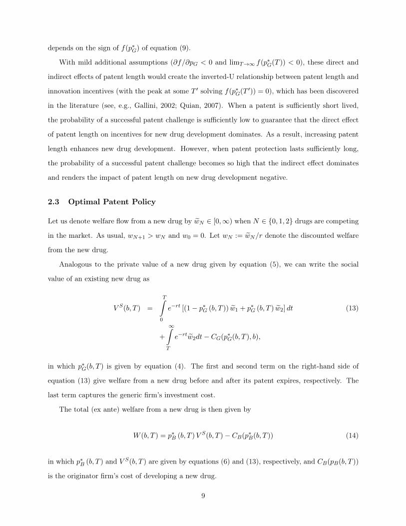
Analogous to the private value of a new drug given by equation (5), we can write the social
value of an existing new drug as
V S(b, T ) =
T∫0
e−rt [(1− p∗G (b, T )) w̃1 + p∗G (b, T ) w̃2] dt (13)
+
∞∫T
e−rtw̃2dt− CG(p∗G(b, T ), b),
in which p∗G(b, T ) is given by equation (4). The first and second term on the right-hand side of
equation (13) give welfare from a new drug before and after its patent expires, respectively. The
last term captures the generic firm’s investment cost.
The total (ex ante) welfare from a new drug is then given by
W (b, T ) = p∗B (b, T )V S(b, T )− CB(p∗B(b, T )) (14)
in which p∗B (b, T ) and V S(b, T ) are given by equations (6) and (13), respectively, and CB(pB(b, T ))
is the originator firm’s cost of developing a new drug.
9

Following the standard practice, we determine the socially optimal combination of patent length
and scope in the pharmaceutical industry by maximizing the social surplus from a new drug, keeping
incentives for new drug development fixed at a desired level pB. The regulator’s problem can thus
be expressed as
maxb∈[0,∞), T∈[0,∞)
V S(b, T )
subject to
p∗B (b, T ) = pB. (15)
Recalling that εb > 0 (Assumption 1) the optimal patent policy can be characterized as follows:
Proposition 3: i) If f(p∗G) < 0, it is optimal to reduce both patent length and patent scope; ii)
If εb > f(p∗G) > 0, it is optimal to reduce patent length and increase patent scope; iii) If f(p∗G) > εb,
it is optimal to reduce patent scope and increase patent length.
Proof: In Appendix A.1.
We may explain Proposition 3 as follows: If εb > f(p∗G), short-lived patents are optimal irre-
spective of the sign of f(p∗G). This result tends to arise from the models of costly imitation. In our
context, a possibility to challenge new drug patents makes longer patent duration an inefficient way
to promote new drug development, since it also increases incentives for patent challenging.
When short-lived patents are optimal, the sign of f(p∗G) > 0 determines the optimal direction
of adjusting patent scope. If f(p∗G) > 0, shorter patent length has an adverse effect on incentives to
develop new drugs and it should be compensated by making patents broader. If f(p∗G) < 0, patent
challenging is so lucrative that shortening patent length has a positive effect on incentives to develop
new drugs, and patents can be made narrower without jeopardizing new drug development. Thus the
sign of f(p∗G) also determines whether patent length and scope are substitutable or complementary
policy tools with regard to new drug development.
Nonetheless, even in the presence of costly imitation, it is possible that narrow and long-lived
patents are optimal. Here this scenario happens when f(p∗G) > εb. A small εb makes increasing
patent scope less efficient since then it has only a relatively small impact on the generic firm’s patent
challenging incentives but a relatively large impact on its costs. Thus, distortions caused by broader
patents can even be larger than distortions caused by longer patents. It is, however, difficult to
10

come up with a cost function that would generate this outcome.
Example 1. Let us assume that the generic firm’s cost function has a constant elasticity, and
takes the form
CG(pG, b) =c(b)pηGGηG
, (16)
in which ηG > 1 is a constant capturing the elasticity of the cost function, and c(b) ≥ 0 denotes
a constant scaling the cost function. Assume that this constant is an increasing function of patent
scope, ∂c/∂b > 0.
The cost function specified by equation (16) implies that Assumption 1 holds and, as a result,
Propositions 1 and 2 also hold with respect to patent scope.
As to the optimal policy, equation (16) implies that εp = ηG − 1 and we can rewrite equation
(9) as
f(pG) = ηG −1
1− pG. (17)
Since ∂CG/∂b = (∂c/∂b)pηGG /ηG and ∂C2G/∂pG∂b = (∂c/∂b)pηG−1G , εb = ηG. As a result, εb > f(pG).
Thus, by Proposition 3, short-lived patents are optimal irrespective of the sign of f(pG). However,
the sign of f(pG) determines the sign of ∂p∗B/∂T and solves the question of whether patent scope
should be made broader or narrower to neutralize the effect of shorter patent duration on the
incentives to develop new drugs.
2.4 Implications for Empirical Analysis
The theoretical model suggests several hypotheses that can be evaluated by merely using data on
the generic firms’ challenges to new drug patents: First, the model – like other models of costly
imitation – predicts that ∂p∗G/∂T > 0. If ∂p∗G/∂T > 0 holds in our data, then designing the optimal
patent length for the pharmaceutical industry should take into account the additional distortions
arising from enhanced incentives for patent challenging.
Second, we determine the sign of ∂p∗G/∂b in our data. Based on the literature, we use multiple
measures of patent scope in our empirical analysis. A good measure of patent scope should almost
by definition imply that ∂p∗G/∂b < 0. Furthermore, if ∂p∗G/∂b < 0 based on some measure of patent
scope, then that measure of patent scope could be used neutralize the effect of a change in patent
length on incentives to develop new drugs.
11
Third, according to our results, the effect of a change in patent length on incentives to develop
new drugs depends on the sign of f(p∗G) := εp−p∗G(1−p∗G). Establishing the sign of f(p∗G) also tells
whether patent length and scope are substitutable or complementary policy tools. Our data gives
a direct estimate of p∗G. To recover εp, we develop two approaches: one based on the point estimate
of ∂p∗G/∂T and another based on the point estimate of ∂p∗G/∂b. These point estimates also allow us
to assess whether εb is larger or smaller than f(p∗G), and thereby to complete the characterization
of the optimal patent policy.
3 Construction of Data and Variables
To characterize optimal patent policy for pharmaceutical industry, we measure generic entry prior
to the expiration of new drug patents, and the responses of that entry to changes in effective patent
length and in patent scope.
The FDA is our source of the data concerning patents protecting approved new drugs, generic
entry before patent expiration, and new drug characteristics. We obtain information on patent
attributes from the USPTO and the European Patent Office (EPO). We next explain the construc-
tion of variables used in our main regressions. Appendices 2–4 contain further details of our data
sources, the dataset development, and the description of variables used in robustness checks.
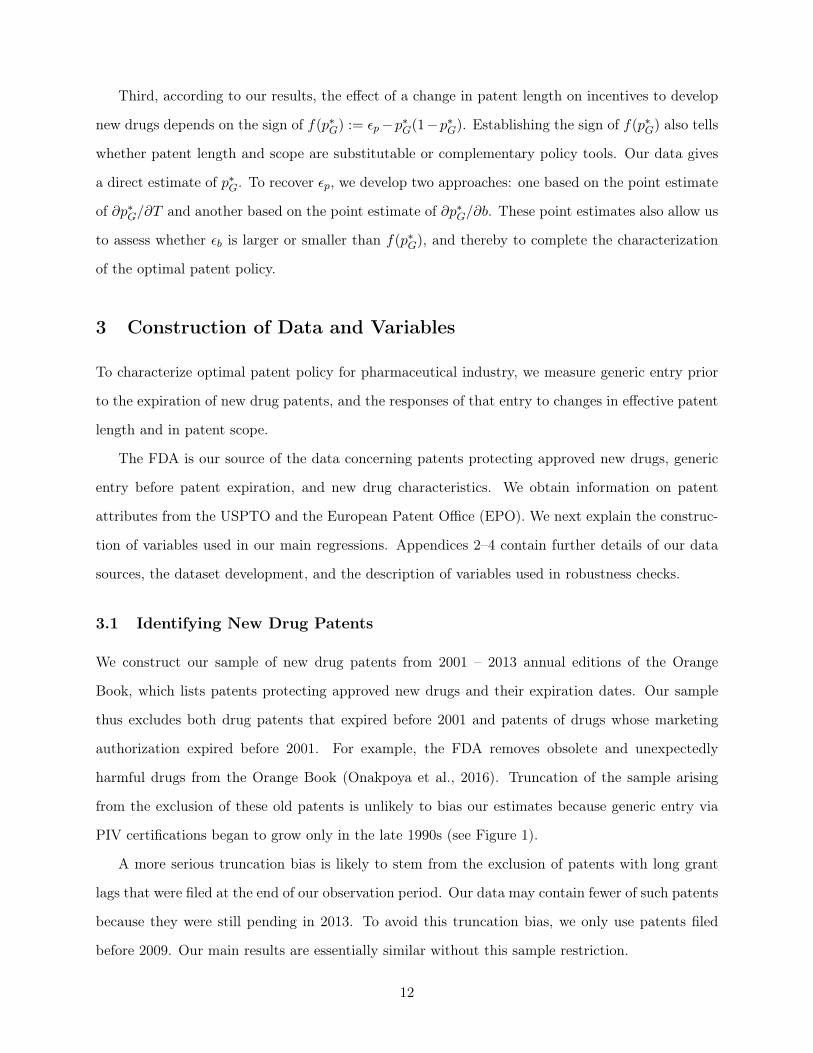
3.1 Identifying New Drug Patents
We construct our sample of new drug patents from 2001 – 2013 annual editions of the Orange
Book, which lists patents protecting approved new drugs and their expiration dates. Our sample
thus excludes both drug patents that expired before 2001 and patents of drugs whose marketing
authorization expired before 2001. For example, the FDA removes obsolete and unexpectedly
harmful drugs from the Orange Book (Onakpoya et al., 2016). Truncation of the sample arising
from the exclusion of these old patents is unlikely to bias our estimates because generic entry via
PIV certifications began to grow only in the late 1990s (see Figure 1).
A more serious truncation bias is likely to stem from the exclusion of patents with long grant
lags that were filed at the end of our observation period. Our data may contain fewer of such patents
because they were still pending in 2013. To avoid this truncation bias, we only use patents filed
before 2009. Our main results are essentially similar without this sample restriction.
12

Long grant lags could also cause a reverse distortion at the beginning of our observation period
if a patent was filed before 1980, but our data contains only 14 such patents. We drop all patents
with grant lags exceeding five years in robustness analyses. Our final sample consists of 3517 new
drug patents granted between 1980 – 2013 and listed in the Orange Book.
3.2 Measuring Generic Entry via Patent Challenges
Our outcome variable is an indicator for whether a new drug patent listed in the Orange Book has
successfully been challenged via PIV certification at least once. In a PIV challenge, a generic firm
seeks to enter prior to the expiration of a new drug patent listed in the Orange book by filing an
FDA application containing a certification that the new drug patent is invalid, unenforceable, or
noninfringed by the generic product (FDA, 2004).
We obtain a list of 1020 approved generic drugs with a PIV certification from the FDA. The list,
however, contains no patent information. To identify the successfully challenged new drug patents,
we read the FDA’s generic drug approval letters. Some of the approval letters are readily available
from the Drugs@FDA database. We obtain more approval letters by submitting the Freedom of
Information Act requests to the FDA. However, we fail to specify the challenged patents for 343
approved generic drugs with a PIV certification.
Although the missing patent observations may lead to an underestimate of the number of success-
ful PIV challenges at a patent level, the measurement error in our outcome variable, the indicator for
at least one successful challenge of a patent via PIV certification, is likely to be small. To measure
the outcome variable accurately, it suffices to observe only one of potentially many successful PIV
challenges. Moreover, when we aggregate the successful challenges to the active ingredient level,
we almost always observe a corresponding challenged patent in our sample. We provide further
arguments for why missing patent information is unlikely to bias the results in Appendix 2.
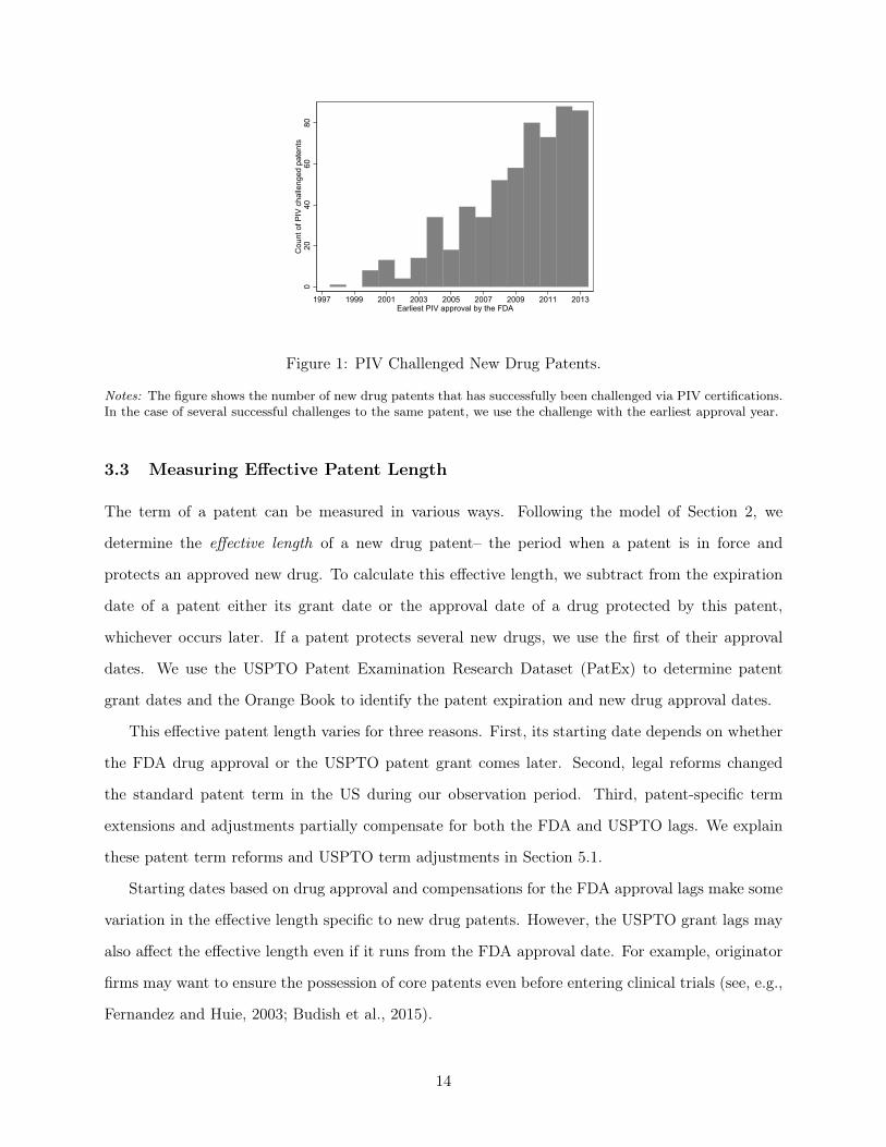
Figure 1 depicts the number of originator drug patents successfully challenged via PIV certifi-
cations in our sample by the generic entry year. If we observe multiple successful PIV challenges
of the same new drug patent, we use the one with the earliest generic drug approval date. While
using a different measure, Figure 1 confirms the finding documented by Branstetter et al. (2016)
that generic entry via PIV certifications became de facto possible only after a series of legal and
policy changes at the turn of the millennium.
13
020
4060
80C
ount
of P
IV c
halle
nged
pat
ents
1997 1999 2001 2003 2005 2007 2009 2011 2013Earliest PIV approval by the FDA
Figure 1: PIV Challenged New Drug Patents.
Notes: The figure shows the number of new drug patents that has successfully been challenged via PIV certifications.In the case of several successful challenges to the same patent, we use the challenge with the earliest approval year.
3.3 Measuring Effective Patent Length
The term of a patent can be measured in various ways. Following the model of Section 2, we
determine the effective length of a new drug patent– the period when a patent is in force and
protects an approved new drug. To calculate this effective length, we subtract from the expiration
date of a patent either its grant date or the approval date of a drug protected by this patent,
whichever occurs later. If a patent protects several new drugs, we use the first of their approval
dates. We use the USPTO Patent Examination Research Dataset (PatEx) to determine patent
grant dates and the Orange Book to identify the patent expiration and new drug approval dates.
This effective patent length varies for three reasons. First, its starting date depends on whether
the FDA drug approval or the USPTO patent grant comes later. Second, legal reforms changed
the standard patent term in the US during our observation period. Third, patent-specific term
extensions and adjustments partially compensate for both the FDA and USPTO lags. We explain
these patent term reforms and USPTO term adjustments in Section 5.1.
Starting dates based on drug approval and compensations for the FDA approval lags make some
variation in the effective length specific to new drug patents. However, the USPTO grant lags may
also affect the effective length even if it runs from the FDA approval date. For example, originator
firms may want to ensure the possession of core patents even before entering clinical trials (see, e.g.,
Fernandez and Huie, 2003; Budish et al., 2015).
14

3.4 Measuring Patent Scope
There are many different measures of patent scope (breadth). We identify several measures of
patent claim scope from the USPTO Patent Claims Research Dataset. We calculate the count of
"Markus groups" in the first independent claim. Drug patent claims often include such Markush
groups – lists of functionally equivalent alternatives (see, e.g., Kuhn and Thompson, 2019). The
count of Markush groups in the first independent claim of a patent might reflect different potential
uses of the drug protected by the patent, and hence its scope. A common and acceptable form of a
Markush group is “...selected from the group consisting of A, B, and C.”.4 We thus use the count
of the phrase "selected from" in the first independent claim as a proxy for the count of Markush
groups. (We get similar results if we use the phrase "consisting of" as a proxy for a Markush group).
We also calculate the count of "or" in the first independent claim, since the coordinating con-
junction "or" might be used to introduce variants or different elements of the drug protected by the
patent. In addition, we calculate the count of words in the first independent claim. Some studies
(e.g., Okada et al., 2016; Kuhn and Thompson, 2019; Marco et al., 2019) use the number of words
in claims as an inverse proxy for patent scope. However, Kuhn and Thompson (2019) argue that
the use of Markush groups reverses this inverse relationship between claim length and scope in the
case of pharmaceutical patents. Following, e.g., Lanjouw and Schankerman (2001, 2004) and Marco
et al. (2019), we also use the number of independent claims as a proxy for patent scope.
Measures of patent claim scope are frequently used in the literature since they are easy to
construct and their legal foundations are clear: the purpose of patent claims is to set out "the
metes and bounds" of the patent rights (e.g., Merges and Nelson, 1990 and Freilich, 2015). In our
case, another advantage of claim scope measures is that we can formulate patent-examiner specific
instruments in an attempt to identify the effects of patent scope on PIV patent challenges (see
Section 6). Yet, measures of claim scope are at best imperfect proxies for patent scope and, at
worst, it is ambiguous whether a change in a claim scope measure (e.g., an additional claim or
word) makes a patent broader or narrower. We thus also seek alternative proxies for patent scope.
Using the Orange Book, we create dummies measuring whether or not a patent in our sample
protects a drug with new chemical entity (NCE), orphan drug, or pediatric exclusivity. These4See, e.g., the USPTO Manual of Patent Examining Procedure (9th edition) §803.02, https://www.uspto.gov/
web/offices/pac/mpep/s803.html#d0e98237, last accessed on February 5, 2020.
15

exclusivities are granted by the FDA upon approval of the drug, and they prevent generic companies
from using clinical trials data from the original products, making generic entry all but prohibitively
costly during the exclusivity period (see, e.g., Yin, 2017). NCE exclusivity last four to five years, and
orphan drug exclusivity seven years. These exclusivities thus should make a drug patent stronger
compared to patents with no exclusivity or with the three year clinical investigation exclusivity.
Pediatric drugs may get six months of exclusivity on the top of other exclusivity periods and the
patent term. Pediatric exclusivity thus makes patent protection both broader and longer.
Finally, we create dummies measuring whether a patent in our data covers an active ingredient,
a method of use, or some other pharmaceutical invention (e.g., drug formulation or composition).
Active ingredient patents might provide stronger protection than other types of new drug patents
(Hemphill and Sampat, 2011b). As detailed in Appendix 2, we infer these patent properties from the
abstracts and claims of patents by using text pattern recognition algorithm and manual verification.
3.5 Other Patent Characteristics
We control for several characteristics of our sample patents and of the drugs protected by those
patents. We determine from the Orange Book whether a patent protects a drug that is available
as a capsule, an injection, a tablet or in some other, less common form. A dosage form may affect
generic firms’ incentives to engage in PIV challenges, since some dosage forms may be easier, e.g., to
manufacture or to distribute to consumers, or to use by consumers. From the Drugs@FDA database,
we identify whether a patent protects a drug priority reviewed by the FDA. Such priority reviews
may reflect drug value.
We collect data on backward and forward patent citations from the USPTO Patent Full-Text
and Image Database (PatFT), and on patent family size from the Open Patent Services of the
EPO. Patent family size and citations are commonly used indicators of patent value (Lanjouw
and Schankerman, 2004; Gambardella et al., 2008). Backward citations could also serve as proxy
for patent scope: for example, careful documentation of prior art can make a patent difficult to
invalidate on the grounds of failure to disclose prior art (Lanjouw and Schankerman, 2001; Harhoff
and Reitzig, 2004). However, a high number of backward citations may also indicate a patent
protecting an incremental invention, which could make the patent less lucrative for PIV challenges.
From PatEx, we identify patents filed as continuation, continuation-in-part or divisional appli-
16

cations. Such "continuing patents" may differ from other patents across various dimensions (Lemley
and Moore, 2004) that may affect propensity to encounter PIV challenges.
We retrieve the main three-digit U.S. Patent Classification (USPC) number and the filing year of
each patent in our sample from PatEx, and use them as fixed effects to control for technology specific
idiosyncrasies and time trends in patenting. To account for possible negative bias in our length
estimates due to different exclusivity periods, we construct fixed effects for the latest exclusivity
expiration year (obtained from the Orange Book).5 To cluster the regression standard errors, we
identify from the Orange Book the first FDA-approved active ingredient related to each patent.
3.6 Summary Statistics
Table 1 reports the summary statistics for our sample of 3517 new drug patents. Over 17 percent of
these patents have been successfully challenged by generic firms via PIV certifications. The effective
length of pharmaceutical patents is on average almost 13 years, varying from one month to 20 years.
A new drug patent has three independent claims on average. An average first independent claim
contains one Markush group and 117 words of which three are the conjunction "or". The average
numbers of backward and forward citations are both roughly around 35, and the mean patent family
size is 13. All count variables have highly skewed distributions.
Half of the patents in our sample protect a drug covered by either NCE exclusivity or orphan drug
exclusivity. Furthermore, pediatric exclusivity is attached to 18 percent of the patents. Approxi-
mately 23 percent of the patents concern active ingredients and 31 percent concern new methods
of use. A majority of the patents are filed as continuing applications. Around 20 percent of the
patents protect injectable drugs, 16 percent capsules, 38 percent tablets, and around eight percent
protect drugs priority reviewed by the FDA.5When constructing these fixed effects for the latest exclusivity expiration year, we group together patents pro-
tecting a drug for which we observe no exclusivity. This group includes both drugs for which the FDA never awardedexclusivity and drugs whose exclusivity expired before 2001 (the beginning of our observation period). Our resultsremain similar when estimated using the sample of patents protecting drugs for which we observe exclusivity (seeTable 7 in Appendix A.3).
17

Table 1: Summary Statistics for New Drug Patents.
Mean Std. Dev. Min Max NPIV entry 0.171 0.377 0 1 3517Effective length 12.586 3.931 0.096 20 3517Markush groups 0.704 4.151 0 112 3485Conjuctions "or" 3.256 9.572 0 184 3485Words 116.890 153.337 1 2197 3485Independent claims 3.187 3.840 1 92 3488NCE exclusivity 0.374 0.484 0 1 3517Orphan drug exclusivity 0.123 0.328 0 1 3517Pediatric exclusivity 0.177 0.382 0 1 3517Method patent 0.311 0.463 0 1 3517Active ingredient patent 0.226 0.419 0 1 3517Forward citations 35.705 57.889 0 1297 3517Backward citations 34.065 63.209 0 1005 3517Patent family size 13.418 12.031 1 51 3511Continuing patent 0.589 0.492 0 1 3517Priority review 0.078 0.269 0 1 3517Tablet 0.384 0.486 0 1 3517Capsule 0.160 0.366 0 1 3517Injectable 0.195 0.397 0 1 3517
Notes: This table reports summary statistics for our sample of 3517 new drugpatents. PIV entry equals 0 if a patent has never been successfully challenged viaa PIV certification, and 1 otherwise. Effective length is measured in years anddefined as "Expiration date - max{Grant date, Drug approval date}". The third,fourth and fifth row depict the counts of Markush groups, conjunctions "or", andwords, respectively, in the first independent claim. Each exclusivity indicatorequals 1 if a patent covers a drug that has been awarded the correspondingexclusivity. The indicators Method patent and Active ingredient patent equal 1if a patent protects a method of use and an active ingredient, respectively. Theindicators Tablet, Capsule, and Injectable equal 1 if the drug protected by apatent has the corresponding dosage form. The Priority review indicator equals1 if a patent has been priority reviewed by the FDA, and the Continuing patentindicator equals 1 if a patent is filed as a continuation, a continuation-in-partor a divisional application. Independent claims, Backward citations, Forwardcitations, and Patent family size give the count of independent claims includedin a patent in our sample, of earlier patents cited by a patent in our sample, oflater patents citing a patent in our sample, and of countries where the same newdrug has been patented, respectively.
18
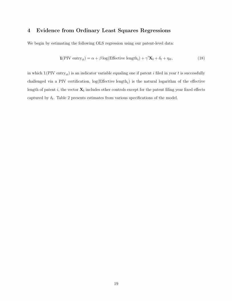
4 Evidence from Ordinary Least Squares Regressions
We begin by estimating the following OLS regression using our patent-level data:
1(PIV entryit) = α+ β log(Effective lengthi) + γ′Xi + δt + ηit, (18)
in which 1(PIV entryit) is an indicator variable equaling one if patent i filed in year t is successfully
challenged via a PIV certification, log(Effective lengthi) is the natural logarithm of the effective
length of patent i, the vector Xi includes other controls except for the patent filing year fixed effects
captured by δt. Table 2 presents estimates from various specifications of the model.
19

Table 2: PIV Entry and Patent Characteristics: OLS Estimates.
(1) (2) (3)log(Effective length) 0.129*** 0.069*** 0.065***
(0.015) (0.013) (0.013)NCE exclusivity -0.091*** -0.075***
(0.025) (0.026)Orphan drug exclusivity -0.093*** -0.092***
(0.024) (0.025)Pediatric exclusivity 0.087** 0.086**
(0.035) (0.035)Priority review 0.179*** 0.178***
(0.046) (0.047)Tablet 0.181*** 0.183***
(0.027) (0.028)Capsule 0.106*** 0.112***
(0.034) (0.035)Injectable -0.041* -0.033
(0.024) (0.024)log(Markush groups+1) -0.012
(0.012)Method patent -0.029*
(0.017)Active ingredient patent -0.063***
(0.021)log(Forward citations+1) 0.003
(0.007)log(Backward citations+1) -0.021**
(0.008)log(Patent family size) 0.010*
(0.006)Continuing patent 0.024
(0.015)Mean dep. variable 0.171 0.171 0.173Observations 3517 3517 3483R-squared 0.065 0.224 0.237Filing year FE × × ×Exclusivity expiration year FE × ×USPC FE ×
Notes: This table reports coefficients from OLS regressions of the PIV en-try indicator on log(Effective length), various measures of patent scope andcontrols. FE stands for fixed effects. Standard errors, in parentheses, are clus-tered at the level of patents protecting the same drug. ∗ p < 0.10, ∗∗ p < 0.05,∗∗∗ p < 0.01.
We find a statistically significant but economically modest relationship between PIV entry and
20
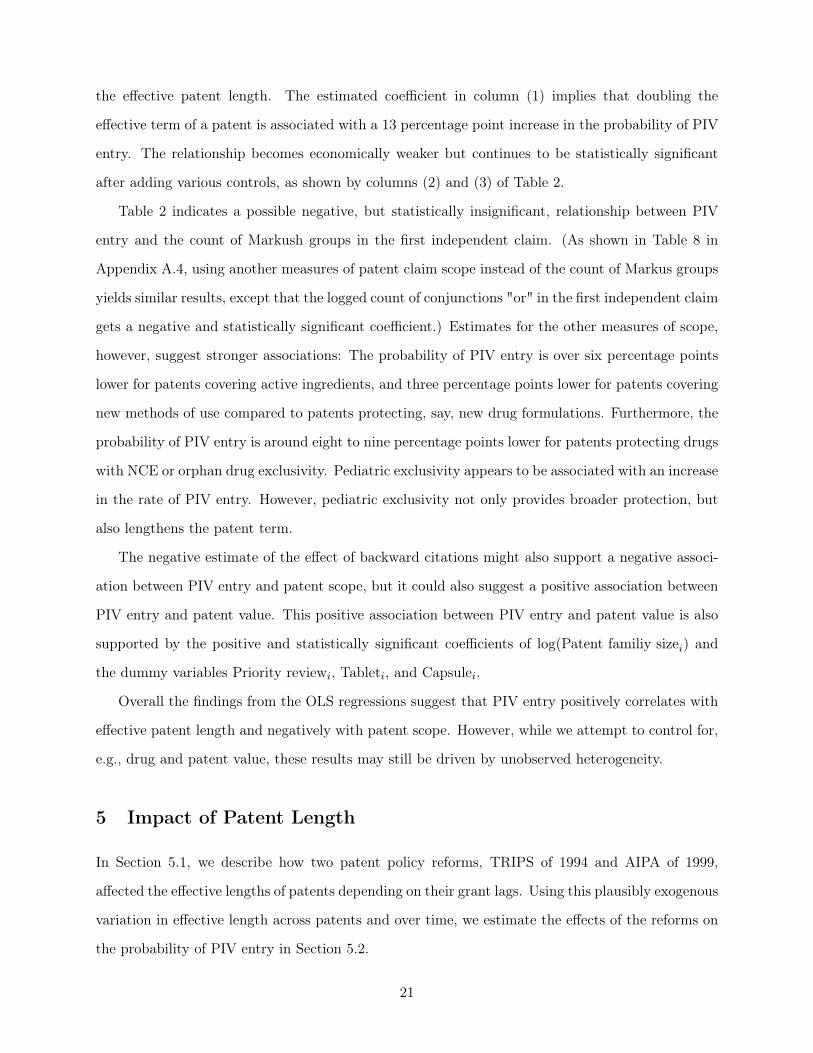
the effective patent length. The estimated coefficient in column (1) implies that doubling the
effective term of a patent is associated with a 13 percentage point increase in the probability of PIV
entry. The relationship becomes economically weaker but continues to be statistically significant
after adding various controls, as shown by columns (2) and (3) of Table 2.
Table 2 indicates a possible negative, but statistically insignificant, relationship between PIV
entry and the count of Markush groups in the first independent claim. (As shown in Table 8 in
Appendix A.4, using another measures of patent claim scope instead of the count of Markus groups
yields similar results, except that the logged count of conjunctions "or" in the first independent claim
gets a negative and statistically significant coefficient.) Estimates for the other measures of scope,
however, suggest stronger associations: The probability of PIV entry is over six percentage points
lower for patents covering active ingredients, and three percentage points lower for patents covering
new methods of use compared to patents protecting, say, new drug formulations. Furthermore, the
probability of PIV entry is around eight to nine percentage points lower for patents protecting drugs
with NCE or orphan drug exclusivity. Pediatric exclusivity appears to be associated with an increase
in the rate of PIV entry. However, pediatric exclusivity not only provides broader protection, but
also lengthens the patent term.
The negative estimate of the effect of backward citations might also support a negative associ-
ation between PIV entry and patent scope, but it could also suggest a positive association between
PIV entry and patent value. This positive association between PIV entry and patent value is also
supported by the positive and statistically significant coefficients of log(Patent familiy sizei) and
the dummy variables Priority reviewi, Tableti, and Capsulei.
Overall the findings from the OLS regressions suggest that PIV entry positively correlates with
effective patent length and negatively with patent scope. However, while we attempt to control for,
e.g., drug and patent value, these results may still be driven by unobserved heterogeneity.
5 Impact of Patent Length
In Section 5.1, we describe how two patent policy reforms, TRIPS of 1994 and AIPA of 1999,
affected the effective lengths of patents depending on their grant lags. Using this plausibly exogenous
variation in effective length across patents and over time, we estimate the effects of the reforms on
the probability of PIV entry in Section 5.2.
21

5.1 Patent Term Reforms in the US and Pharmaceutical Patents
TRIPS introduced a 20-year standard patent term measured from the (earliest) filing date to the
US. Prior to TRIPS, the US had a 17-year standard patent term counting from the grant date. The
change in the standard patent term was implemented so that the 20-year term from filing applies
to the patents filed on and after June 8, 1995. For patents filed prior to June 8, 1995, the standard
patent term was changed to either the new 20-year term from filing or the old 17-year term from
the grant, whichever expires later. (Patents that were issued prior to June 8, 1978, were kept in the
old 17-year term regime, but our sample includes no such old patents.)
This change in the standard patent term due to TRIPS treats patents differently depending on
whether or not they are granted within three years from filing: Patents granted within three years
from filing receive the same 20-year standard term from filing regardless of whether or not they
are filed before or after TRIPS (came into force). In contrast, patents with grant lags exceeding
three years filed before TRIPS received the 17-year standard term from the grant date, which fully
compensates for grant lags. But similar patents filed after TRIPS receive the 20-year standard term
from filing, thus losing some of effective protection time because of TRIPS.
To compensate patentees for this loss in effective patent life because of delays in the USPTO
approval process, TRIPS also introduced PTAs (which were initially called patent term extensions).
These PTAs only apply to patents filed after TRIPS, and can add a maximum of five years to the
patent term. The USPTO calculates the length of a PTA automatically, taking into account only
certain delays caused by the USPTO itself. Initially eligible delays were limited (to interference,
secrecy orders, successful appeals to the Patent Trial and Appeal Board or to the federal courts)
but, subsequently, AIPA expanded the list of reasons which may give rise to PTAs for patents filed
on and after May 29, 2000. In particular, AIPA introduced compensation for grant lags exceeding
three years, thus at least partially neutralizing the adverse impact of TRIPS on the length of patents
with grant lags exceeding three years.
We determine PTAs and grant lags for our sample of drug patents from PatEx. As shown by
panels A and B of Figure 2, PTAs were rare and their duration was short before AIPA (came into
force), which increased their provision substantially. The share of patents with a PTA rises from two
percent in 1996 to 66 percent in 2005 in our sample (panel A). The average PTA length increases
from less than a month in 1996 to around 15 months in 2005 (panel B). Even after AIPA, the
22

increase in the length of PTAs was gradual, reflecting increasingly slow patent prosecution at the
USPTO in the early years of the millenium (panel C). (The long grant lags observed in the early
years in panel C are a consequence of the truncation of our sample discussed in Section 3.1).
0.2
.4.6
.8S
hare
of p
aten
ts w
ith a
US
PTO
term
adj
ustm
ent
1990 1995 2000 2005 2010Patent filing year
A Share of Patents with a USPTO PTA
0.5
11.
5A
vera
ge U
SP
TO te
rm a
djus
tmen
t (ye
ars)
1990 1995 2000 2005 2010Patent filing year
B Average PTA Length
11.
52
2.5
33.
54
4.5
Ave
rage
gra
nt la
g (y
ears
)
-1980 1985 1990 1995 2000 2005 2010Patent filing year
C Average Grant Lag
Figure 2: USPTO Grant Lags and PTAs of Pharmaceutical Patents.
Notes: Panel A of this figure shows the share of new drug patents in our sample with a USPTO PTA by patentfiling year. Panel B shows the average length of a PTA in our sample by patent filing year, including patents withoutPTAs. Panel C figure shows the average grant lag of new drug patents in our sample by patent filing year.
Comparing panels A and B with panel C indicates that PTAs fail to fully compensate for the
adverse impact of TRIPS on the effective length of new drug patents with long grant lags, especially
before AIPA. To confirm this suggestion, we regress the patent grant lag on the effective patent
length separately for the periods of pre-TRIPS, post-TRIPS but pre-AIPA, and post-AIPA. Figure 3
shows the results: Before TRIPS, the effective length is relatively invariant to the grant lag. TRIPS
disproportionately shortens the effective length of patents that were pending more than three years,
especially before AIPA, which partially restores the effective length of such patents.
23

-4-2
02
4E
ffect
ive
pate
nt le
ngth
<1.5 [1.5,2) [2,2.5) [2.5,3) [3,3.5) [3.5,4) [4,4.5) [4.5,5) 5-Patent grant lag
Pre-TRIPS Post-TRIPS, pre-AIPAPost-AIPA
Figure 3: Effective Patent Length Before and After TRIPS and AIPA.
Notes: This figure shows relationships between the patent grant lag (in the x-axes) and the effective patent length(in the y-axis). We estimate the relationships separately for three time periods by using OLS and our patent-leveldata. The pre-TRIPS period includes patents filed before June 8, 1995. The pre-TRIPS, post-AIPA period includespatents filed between June 8, 1995 and May 29, 2000. The post-AIPA period includes patents filed on or after May29, 2000. In each regression, the comparison group consists of patents granted less than 1.5 years from the filing date.Each dot shows the averages of the x- and y-axes variables within each equal-sized bin.
5.2 Difference-in-Differences Estimations and Results
In Section 5.1 we document how patents with grant lags exceeding three years have shorter effective
lengths than other patents after TRIPS. The model of Section 2 predicts an increase in the rate of
PIV entry encountered by such patents after TRIPS. Furthermore, this positive effect of TRIPS on
the rate of PIV entry should be stronger before AIPA than after it. Consistent with this prediction,
Figure 4 indicates that in the post-TRIPS, pre-AIPA period, the rate of PIV entry is lower for
patents prosecuted over three years compared to patents with shorter grant lags. There is no
similar difference between the two patent groups in other periods. These patterns in grant lags and
PIV entry motivate our research design.
24

TRIPS AIPA
0.1
.2.3
.4A
vera
ge P
IV e
ntry
-1990 1995 2000 2005 2010Filing year
Grant lag < 3 years Grant lag ≥ 3 years
Figure 4: Average PIV Entry by Patent Filing Year and Grant Lag.
Notes: This figure shows the average PIV entry by patent filing year. The dashed and solid lines depict the groupsof patents with a grant lag more and less than three years, respectively. The year 1990 also includes all patentsfiled before it. Those oldest patents in our sample encounter only few successful PIV challenges with no systematicdifference depending on the grant lag.
We estimate the following DiD model using our patent-level data:
1(PIV entryit) = α+ β11(Grant lagi ≥ 3years) + (19)
β21(Grant lagi ≥ 3years)× 1(Post-TRIPSit) +
β31(Grant lagi ≥ 3years)× 1(Post-AIPAit) + γ′Xi + δt + εit,
in which 1(Grant lagi ≥ 3years) is an indicator variable equaling one if patent i filed in year t has
at least a three-year grant lag, 1(Post-TRIPSit) is an indicator variable equaling one if the filing
date of patent i is on or after June 8, 1995, and 1(Post-AIPAit) is an indicator variable equaling
one if the filing date of patent i is on or after May 29, 2000. The coefficients of interest, β2 and β3,
measure changes in the probability of PIV entry after TRIPS and AIPA, respectively, for patents
prosecuted at least three years (treatment group), compared to other patents (control group).
25
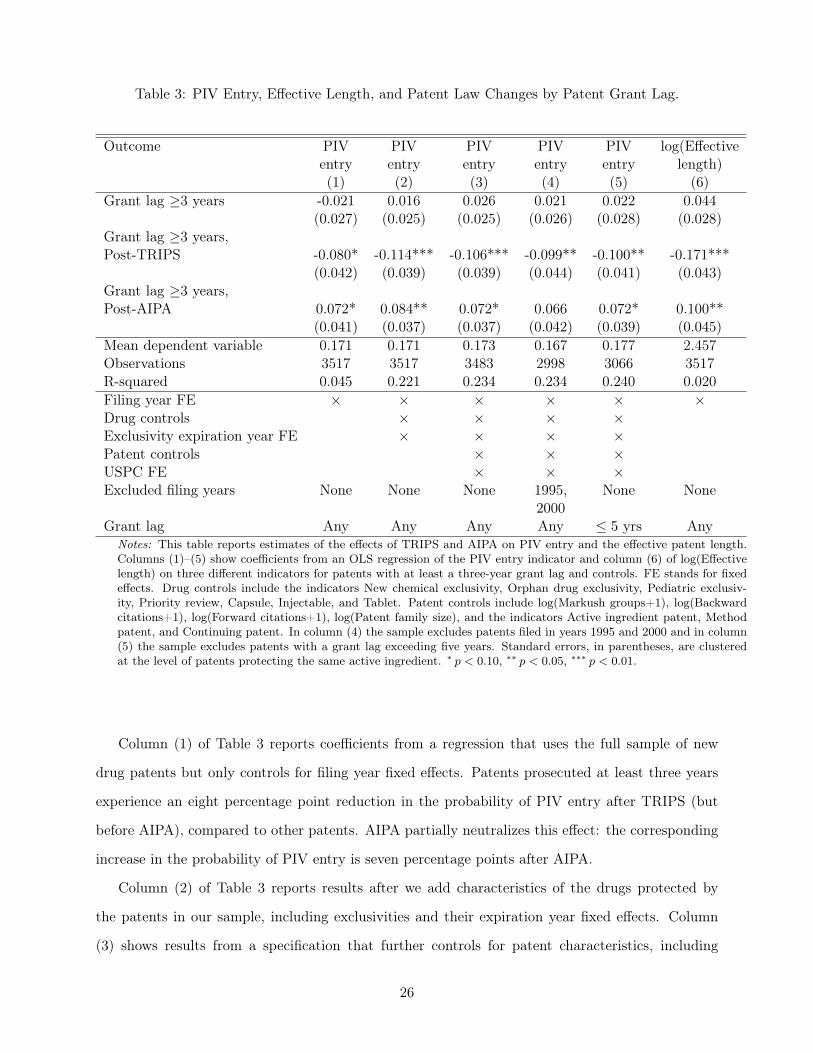
Table 3: PIV Entry, Effective Length, and Patent Law Changes by Patent Grant Lag.
Outcome PIV PIV PIV PIV PIV log(Effectiveentry entry entry entry entry length)(1) (2) (3) (4) (5) (6)
Grant lag ≥3 years -0.021 0.016 0.026 0.021 0.022 0.044(0.027) (0.025) (0.025) (0.026) (0.028) (0.028)
Grant lag ≥3 years,Post-TRIPS -0.080* -0.114*** -0.106*** -0.099** -0.100** -0.171***
(0.042) (0.039) (0.039) (0.044) (0.041) (0.043)Grant lag ≥3 years,Post-AIPA 0.072* 0.084** 0.072* 0.066 0.072* 0.100**
(0.041) (0.037) (0.037) (0.042) (0.039) (0.045)Mean dependent variable 0.171 0.171 0.173 0.167 0.177 2.457Observations 3517 3517 3483 2998 3066 3517R-squared 0.045 0.221 0.234 0.234 0.240 0.020Filing year FE × × × × × ×Drug controls × × × ×Exclusivity expiration year FE × × × ×Patent controls × × ×USPC FE × × ×Excluded filing years None None None 1995, None None
2000Grant lag Any Any Any Any ≤ 5 yrs Any
Notes: This table reports estimates of the effects of TRIPS and AIPA on PIV entry and the effective patent length.Columns (1)–(5) show coefficients from an OLS regression of the PIV entry indicator and column (6) of log(Effectivelength) on three different indicators for patents with at least a three-year grant lag and controls. FE stands for fixedeffects. Drug controls include the indicators New chemical exclusivity, Orphan drug exclusivity, Pediatric exclusiv-ity, Priority review, Capsule, Injectable, and Tablet. Patent controls include log(Markush groups+1), log(Backwardcitations+1), log(Forward citations+1), log(Patent family size), and the indicators Active ingredient patent, Methodpatent, and Continuing patent. In column (4) the sample excludes patents filed in years 1995 and 2000 and in column(5) the sample excludes patents with a grant lag exceeding five years. Standard errors, in parentheses, are clusteredat the level of patents protecting the same active ingredient. ∗ p < 0.10, ∗∗ p < 0.05, ∗∗∗ p < 0.01.
Column (1) of Table 3 reports coefficients from a regression that uses the full sample of new
drug patents but only controls for filing year fixed effects. Patents prosecuted at least three years
experience an eight percentage point reduction in the probability of PIV entry after TRIPS (but
before AIPA), compared to other patents. AIPA partially neutralizes this effect: the corresponding
increase in the probability of PIV entry is seven percentage points after AIPA.
Column (2) of Table 3 reports results after we add characteristics of the drugs protected by
the patents in our sample, including exclusivities and their expiration year fixed effects. Column
(3) shows results from a specification that further controls for patent characteristics, including
26

the main US patent class fixed effects. These two specifications attempt to account for potential
differences between the treatment and control groups stemming from observable characteristics,
unobserved heterogeneity, and possible compositional changes over time across these groups. Adding
the fixed effects and other controls makes the effects of TRIPS and AIPA stronger and more precisely
estimated compared to column (1).
We also estimate equation (19) using a sample that excludes patents filed in 1995 and 2000. This
sample restriction attempts to address the potential bias arising from anticipation of the TRIPS
and AIPA reforms. For example, applicants expecting a decrease in patent terms due to TRIPS
could have advanced patent filing and, analogously, applicants expecting an increase in patent terms
due to AIPA could have postponed filing. The coefficient estimates from this regression, reported
in column (4) of Table 3, remain similar to the baseline estimates, suggesting no clear anticipation
effects. The coefficient β3 is, however, less precisely estimated, perhaps due to a smaller sample.
Next, we estimate the DiD model of equation (19) using a sample of patents prosecuted within
five years. This sample restriction further mitigates the concerns arising from possible compositional
changes in the treatment group. For example, exceptionally long grant lags observed in the earliest
and the latest years of our data increase the number of patents falling into the treatment group (see
panel C of Figure 2). This restriction also excludes the patents for which the five-year maximum
length of PTAs is binding. The results from this estimation reported in column (5) are similar to
the baseline results.
To measure the effect of TRIPS and AIPA on the effective patent length, we also estimate an
analogous DiD model to equation (19) in which we replace 1(PIV entryit) by log(Effective patent lengthi)
as an outcome variable. The results reported in column (6) of Table 3 show that patents prosecuted
at least three years experience a 17 percent decrease in their effective term after TRIPS, compared
with other patents. After AIPA the effective length of these patents increases by 10 percent.
Robustness. Overall, we find that the probability of PIV entry increases with effective patent
length, as predicted by the theory: TRIPS shortens the effective length of patents with long grant
lags, and this shortened effective length discourages PIV entry, whereas AIPA partially restores the
effective length of those patents which promotes PIV entry.
To assess the robustness of these findings, we make a number of further checks, some of which
are detailed in Appendix A.3. There we show that the estimated effects on the probability of PIV
27

entry cannot be explained by differential changes in patent scope or value after TRIPS and AIPA,
nor by the introduction of provisional applications in 1995. When we estimate equation (19) using
different subsamples and specifications, the effects of TRIPS and AIPA only become stronger and
more precisely estimated.
We find additional evidence of longer effective patent length encouraging PIV entry: TRIPS
disproportionately shortened effective terms of continuing patents, leading to a more negative es-
timate of β2 using the sample of these patents. Finally, we document how AIPA also mandated
earlier disclosure of patent applications, resulting in a longer period of public patent applications.
This change may affect the interpretation of the effective patent length in the post-AIPA period.
6 Impact of Patent Scope
In identifying the effect of a change in patent scope on PIV patent challenges we cannot resort to
an ideal experiment in which some patents are randomly assigned broader protection than other
patents. Inspired by Kuhn and Thompson (2019), Sampat and Williams (2019), and Farre-Mensa
et al. (2020), we instead develop IVs for patent scope based on the "leniency” of patent examiners.
Our approach exploits the differences across examiners in their propensity to grant broader or more
claims as a source of variation in patent scope, together with the assignment of patent applications
to examiners at the USPTO. Previous research (e.g., Cockburn et al., 2003; Lemley and Sampat,
2012) indicates that examiners differ in their decision making which translates into different patent
outcomes. Since patent prosecution typically consists of several rounds of claim rejections and
modifications required by an examiner (Kuhn and Thompson, 2019; Marco et al., 2019), systematic
differences across examiners plausibly generate systematic differences in patent claim scope.
The second stage of our two-stage least squares (2SLS) analysis consists of estimations of equa-
tion (18) using instrumented scope measures. We instrument the following four measures of scope
of a new drug patent: the counts of Markush groups, the coordination conjunctions "or", and words
in the first independent claim, and the count of independent claims. (Kuhn and Thompson, 2019,
too, develop a similar IV for the count of words in the first independent claim.) For each scope
measure xijt of new drug patent i reviewed by examiner j and filed in year t, we construct the
corresponding instrument zijt as
28
zijt =
t−1∑τ=τ j
njτ∑k=1
xkjτ
t−1∑τ=τ j
njτ
, (20)
in which xkjτ is the scope measure of (any type of) patent k reviewed by examiner j and filed in
year τ , njτ denotes the number of patents reviewed by examiner j in filing year τ , and τ j denotes
the earliest filing year of any patent reviewed by examiner j. Hence, zijt gives the "examiner j’s
historical average" – the cumulative average of a scope measure over all patents assigned to examiner
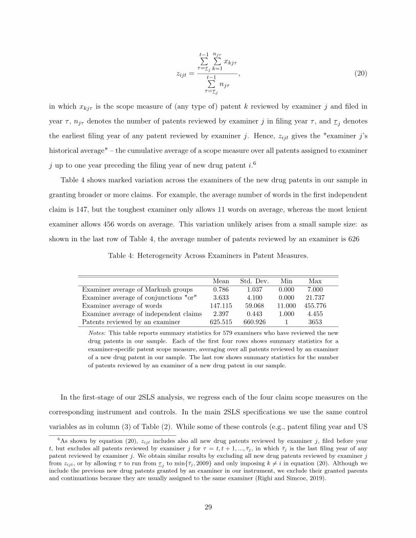
j up to one year preceding the filing year of new drug patent i.6
Table 4 shows marked variation across the examiners of the new drug patents in our sample in
granting broader or more claims. For example, the average number of words in the first independent
claim is 147, but the toughest examiner only allows 11 words on average, whereas the most lenient
examiner allows 456 words on average. This variation unlikely arises from a small sample size: as
shown in the last row of Table 4, the average number of patents reviewed by an examiner is 626
Table 4: Heterogeneity Across Examiners in Patent Measures.
Mean Std. Dev. Min MaxExaminer average of Markush groups 0.786 1.037 0.000 7.000Examiner average of conjunctions "or" 3.633 4.100 0.000 21.737Examiner average of words 147.115 59.068 11.000 455.776Examiner average of independent claims 2.397 0.443 1.000 4.455Patents reviewed by an examiner 625.515 660.926 1 3653
Notes: This table reports summary statistics for 579 examiners who have reviewed the newdrug patents in our sample. Each of the first four rows shows summary statistics for aexaminer-specific patent scope measure, averaging over all patents reviewed by an examinerof a new drug patent in our sample. The last row shows summary statistics for the numberof patents reviewed by an examiner of a new drug patent in our sample.
In the first-stage of our 2SLS analysis, we regress each of the four claim scope measures on the
corresponding instrument and controls. In the main 2SLS specifications we use the same control
variables as in column (3) of Table (2). While some of these controls (e.g., patent filing year and US6As shown by equation (20), zijt includes also all new drug patents reviewed by examiner j, filed before year
t, but excludes all patents reviewed by examiner j for τ = t, t + 1, ..., τ̄j , in which τ̄j is the last filing year of anypatent reviewed by examiner j. We obtain similar results by excluding all new drug patents reviewed by examiner jfrom zijt, or by allowing τ to run from τ j to min{τ̄j , 2009} and only imposing k 6= i in equation (20). Although weinclude the previous new drug patents granted by an examiner in our instrument, we exclude their granted parentsand continuations because they are usually assigned to the same examiner (Righi and Simcoe, 2019).
29

patent class fixed effects) may also capture examiner specialization, we also add USPTO Technology
Center fixed effects. Technology Centers are responsible for examination in broad technological
areas. Each Technology Center typically contains a few dozen Art Units, which are groups of
examiners specializing in narrow technology areas. Within a Technology Center, a patent application
is assigned to an Art Unit and finally to an examiner. We use Technology Center fixed effects instead
of Art Unit fixed effects because we only observe a small number of (eventually granted) new drug
patents per Art Unit.
The exclusion restriction in our setting holds if, conditional on covariates, examiners’ propensity
to grant broader claims is uncorrelated with such application characteristics, e.g., drug or patent
value or quality, that correlate with PIV entry. The validity of this exclusion restriction is supported
by the evidence in, e.g., Lemley and Sampat (2012), Sampat and Williams (2019), Kuhn and
Thompson (2019), and Farre-Mensa et al. (2020), although, e.g., Righi and Simcoe (2019) are more
critical. These previous studies indicate that examiner assignment is independent of application
characteristics at the time of filing. For example, examiner assignment is based on the last digit of the
application number in Art Units. Such assignment plausibly implies that examiner characteristics
are uncorrelated with the value or quality of applications. While Righi and Simcoe (2019) show
that examiners specialize in narrow technology fields, they find no evidence that more valuable
or broader applications are allocated to certain examiners. Moreover, since our new drug patents
form a homogeneous technology field, examiners are less likely to be specialized within this sample.
Nevertheless, the validity of this exclusion restriction is debatable and our IV results must be
interpreted cautiously.
Table 5 reports the 2SLS regression results. The first stage coefficients of panel B and F-statistics
suggest strong instruments. Estimates of the instrumented scope measures of panel A suggest a
negative effect of broader patent scope on the probability of PIV entry: A 10 percentage increase in
the count of Markush groups in the first independent claim decreases the probability of PIV entry
by some two percentage points. Additional words in the first independent claim perform similarly,
supporting the argument advanced by Kuhn and Thompson (2019) about a positive relationship
between claim length and scope in the case of pharmaceutical patents. A 10 percent increase in the
count of conjunctions "or" in the first independent claim makes a successful PIV challenge less likely
by around one percentage point. These coefficients of the scope measures are statistically significant
30

but smaller in magnitude compared to the OLS estimates reported in Table 8 in Appendix A.4. Such
an upward bias in the OLS estimates could arise, e.g., if originator firms seek broader protection
for more valuable drugs which, at the same time, attract more PIV challenges.
Table 5: Patent Scope and PIV Entry: IV Estimates.
(1) (2) (3) (4)PANEL A: Second stage estimatesInstrumented variables:log(Markush groups+1) -0.220**
(0.090)log(Conjunctions "or"+1) -0.105**
(0.052)log(Words) -0.237**
(0.095)log(Independent claims) 0.069
(0.132)PANEL B: First stage estimatesInstruments:log(Examiner historical average of Markush groups+1) 0.239***
(0.048)log(Examiner historical average of conjunctions "or"+1) 0.225***
(0.034)log(Examiner historical average of words) 0.238***
(0.062)log(Examiner historical average of independent claims) 0.242***
(0.073)Observations 3445 3445 3445 3447First stage F-statistic 25.286 44.860 14.523 10.934Technology Center FE × × × ×Filing year FE × × × ×Drug controls × × × ×Exclusivity expiration year FE × × × ×Patent controls × × × ×USPC FE × × × ×
Notes: This table reports the 2SLS estimates of the effects of patent scope on PIV entry. Panel A showsthe main coefficient from the second stage regressions of the PIV entry indicator on the instrumented scopemeasures and controls. Panel B shows the main coefficient from the first stage regressions of the scope measureson the corresponding instruments and controls. The first stage F-statistic test is on the excluded instruments.FE stands for fixed effects. Drug controls include the indicators New chemical exclusivity, Orphan drugexclusivity, Pediatric exclusivity, Priority review, Capsule, Injectable, and Tablet. Patent controls includelog(Effective length), log(Backward citations+1), log(Forward citations+1), log(Patent family size), and theindicators Active ingredient patent, Method patent, and Continuing patent. We use a full sample of newdrug patents for the regressions, and construct the instruments using data on all granted patents reviewed bythe examiners of these new drug patents. Robust standard errors are reported in parentheses. ∗ p < 0.10,∗∗ p < 0.05, ∗∗∗ p < 0.01.
The question of whether or not independent claim count is a useful proxy for patent claim scope
has been debated in the literature (see, e.g., Kuhn and Thompson, 2019 and Marco et al., 2019) for
31

different points of view). Our coefficient estimate of the number of independent claims is close to
zero in magnitude and statistically insignificant, suggesting that additional independent claims in
a pharmaceutical patent fail to protect the patent against PIV challenges.
Robustness. Overall, we view the IV regression results as suggesting that broadening patent
scope hinders PIV entry. We assess the robustness of the results to specification changes in Appendix
A.4. The results remain unchanged when we exclude most of the control variables (Table 9) or
include of an additional control for trends varying with the Technology Center (Table10).
We also use Art Unit fixed effects instead of Technology Center fixed effects (Table 11). The
number of patents per Art Unit is typically small, only 21 on average. Reflecting this challenge, the
point estimates from these specifications remain similar in magnitude compared to the main speci-
fications with Technology Center fixed effects, but are less precisely estimated: only the coefficient
of the word count remains statistically significant at the five percent level.
7 Implications for Patent Policy
Our empirical evidence suggests that longer effective patent length encourages PIV patent chal-
lenges, as predicted by the models of costly imitation. This effect weakens the efficiency of patent
length as a policy tool to promote innovation. Our evidence also suggests that broader patent scope
appears to hinder PIV entry.
However, these findings alone are not enough to characterize the optimal adjustments in patent
length and scope. Ideally, we would also like to know whether or not incentives to develop new
drugs are increasing in patent length. In the absence of a direct test of incentives to develop new
drugs, we resort to the formula f(p∗G) := εp−p∗G/(1−p∗G) developed in Section 2. The sign of f(p∗G)
not only tells us whether incentives to develop new drugs are increasing or decreasing in patent
length but also whether patent length and scope are substitutable or complementary policy tools.
In our data the average probability of PIV entry is 0.17 (see Table 1), which directly provides an
estimate of p∗G.We develop two approaches to recover εp, the elasticity of the generic firms’ marginal
cost function (see equation (1)): one based on the estimated elasticity of PIV entry with respect to
effective patent length, ξT := (∂pG/pG)/(∂T/T ), and another on the corresponding elasticity with
respect to patent scope, ξb := (∂pG/pG)/(∂b/b).
Recovering εp via Patent Length Estimates. In Appendix A.5, we show that εp can be
32

written as
εp =e−rT rT
(1− e−rT )ξT. (21)
Hence, to calculate εp, we need values for r, T and ξT .
We set r = 0.05. The same value of the firms’ discount rate is also used, e.g., by Judd et al.
(2012) in a similar context. Next, since the average effective patent length in our data (see Table
1) is 12.59, we set T = 12.59. These numerical values yield rT ≈ 0.63. Denicolò (2007) suggests
that for an average patent across all industries, rT ∈ [0.6, 1.39].
Finally, to obtain a value for ξT , we compare estimates of β2 of equation (19) in columns (1)–(5)
of Table 3 to the average probability of PIV entry, 0.17. This comparison suggests that TRIPS
reduced the rate of PIV entry by 47-65 percent. These figures, together with the estimated effect of
TRIPS on effective patent length (-17 percent) reported in column (6) of Table 3, suggest that the
elasticity ξT could be between 47/17 ≈ 2.76 and 65/17 ≈ 3.82. We use the mean value of this range
and set ξT = 3.29. Inserting ξT = 3.29, r = 0.05, and T = 12.59 into equation (21) gives εp ≈ 0.22.
Recovering εp via Patent Scope Estimates. Our regressions of the PIV entry indicator on
the logged patent scope measures imply that an estimate of ξb can directly be obtained by dividing
an estimated coefficient of a log scope measure by the average probability of PIV entry, 0.17. The
statistically significant coefficient estimates of the IV regressions (columns (1)–(3) of Panel A of
Table 5) suggest that ξb ∈ [−0.65,−1, 41]. Using the average value of this range, we set ξb = −1.03.
To link ξb with εp, we assume that the generic firm’s cost function has the constant elasticity
form used in Example 1 of Section 2, and further stipulate that c(b) = cb. Using this functional
form, we show in Appendix A.5 that εp = −1/ξb. Thus, setting ξb = −1.03 gives εp ≈ 0.97.
Effect of Patent Length on Incentives to Develop New Drug. We have two alternative
ways to calculate εp in the formula for f(p∗G): using ξT to generate εp yields εp = 0.22, whereas
using ξb yields εp = 0.97. Assuming that these calculations together mean that εp ∈ [0.22, 0.97] and
setting p∗G = 0.17, yields f(p∗G) := εp − p∗G/(1 − p∗G) ∈ [0.02, 0, 77]. To conclude, the marginal cost
of PIV entry appear to be sufficiently inelastic so that innovation incentives in the pharmaceutical
industry are increasing in patent length, implying that patent length and scope are substitutes with
regard to those innovation incentives.
Optimal Patent Policy. To complete the characterization of optimal policy, we should assess
33

whether f(p∗G) is larger or smaller than εb, the elasticity of the effect of patent scope on patent
challenging costs (see equation (2)). We can estimate εb in a similar way as ξb. In Appendix A.5,
we show that εb = 1 − 1/ξb. Using ξb = −1.03 suggests that εb ≈ 1.97. Thus, εb is appears to be
larger than our estimates of f(p∗G). In sum, our results suggest that εb > f(p∗G) > 0, implying that
the term of pharmaceutical patents should be made shorter and this shorter patent term should be
compensated by broader patent scope.
Robustness. Our recommendations concerning the optimal changes to patent length and scope
are based on some strong assumptions. If we base the optimal policy analysis on estimates of the
effect of patent scope, our characterization of optimal policy is robust in the sense that all our
estimates of ξb suggest that f(p∗G) is firmly positive but below εb. However, these estimates are
based on a functional form assumption which we cannot test.
Using patent length estimates to generate the optimal policy recommendations requires no spe-
cific functional form of the generic firm’s cost function, but requires values for the firms’ discount
rate, r, and for the effective patent length, T . Our estimates suggest that f(p∗G) is positive but close
to zero. Hence, equations (9) and (21) imply that somewhat higher values of r, T , or ξT than what
we use would make f(p∗G) negative. For example, using our largest (in absolute value) estimate of
β2 of equation (19) from column (2) of Table 3 would make ξT sufficiently high to render f(p∗G)
slightly negative. (Using any other estimate of β2 keeps f(p∗G) positive.) Moreover, we would get
somewhat smaller estimates of εp (and hence of f(p∗G)), if we used the estimated effects of AIPA in-
stead of those of TRIPS. However, the interpretation of the effect of AIPA on effective patent length
is somewhat ambiguous because of the earlier disclosure of patent applications in the post-AIPA
period (see Appendix A.3).
Finally, a revealed-preference argument supports that f(p∗G) > 0 is more likely than f(p∗G) < 0
– if f(p∗G) were negative, it would be profitable for originator firms themselves to shorten the
effective lengths of their patents. In Appendix A.3 we provide an example of this revealed-preference
argument: we show how originator firms shy away from continuing patents with long grant lags after
TRIPS and argue that such a behavior is consistent with f(p∗G) > 0 but not with f(p∗G) < 0.
We can conclude that f(p∗G) is likely to be small, smaller than εb, but hardly negative.
34

8 Conclusion
We characterize optimal patent policy for the pharmaceutical industry by only using data on phar-
maceutical patents. Our results combining theory and evidence from DiD regressions exploiting
variations in patent law, and IV regressions exploiting patent examiner leniency differences suggest
that new drug patent length should be made shorter, while using broader patent scope to restore
incentives to develop new drugs. The main channel leading to this conclusion is the positive effect
of longer effective patent term on successful PIV patent challenges by generic entrants.
Our IV regression results concern patent claims, but broadening the scope of claims may be an
awkward policy instrument. A more potential policy instrument to broaden pharmaceutical patent
scope could be to restrict PIV challenges, e.g., by providing longer FDA exclusivity periods.
References
Abrams, D. S. (2009). Did trips spur innovation? an empirical analysis of patent duration and
incentives to innovate. University of Pennsylvania Law Review, 157(6):1613–1647.
Belleflamme, P. and Peitz, M. (2015). Industrial Organization: Markets and Strategies. Cambridge
University Press: Cambridge, UK, 2nd edition.
Boldrin, M. and Levine, D. K. (2013). The case against patents. Journal of Economic Perspectives,
27(1):3–22.
Branstetter, L., Chatterjee, C., and Higgins, M. J. (2016). Regulation and welfare: Evidence
from paragraph IV generic entry in the pharmaceutical industry. RAND Journal of Economics,
47(4):857–890.
Budish, E., Roin, B. N., and Williams, H. (2015). Do firms underinvest in long-term research?
evidence from cancer clinical trials. American Economic Review, 105(7):2044–85.
Budish, E., Roin, B. N., and Williams, H. (2016). Patents and research investments: Assessing the
empirical evidence. American Economic Review: Papers & Proceedings, 106(5):183–187.
Cockburn, I., Kortum, S., and Stern, S. (2003). Are all patent examiners equal? Examiners, patent
35

characteristics, and litigation outcomes. In Cohen, W. and Merrill, S., editors, Patents in the
Knowledge-Based Economy, pages 19–53. Washington, DC: The National Academies Press.
Denicolò, V. (1996). Patent races and optimal patent breadth and length. Journal of Industrial
Economics, 44(3):249–265.
Denicolò, V. (2007). Do patents over-compensate innovators? Economic Policy, 22(52):679–729.
Farre-Mensa, J., Hegde, D., and Ljungqvist, A. (2020). What is a patent worth? Evidence from
the U.S. patent “lottery”. Journal of Finance, 75(2):639–682.
FDA (2004). Guidance for industry - listed drugs, 30-month stays, and approval of ANDAs and
505(b)(2) applications under Hatch- Waxman, as amended by the Medicare Prescription Drug,
Improvement, and Modernization Act of 2003 – Questions and Answers. FDA Guidance Docu-
ments.
Fernandez, D. and Huie, J. (2003). Commentaries analyses — strategic balancing of patent and
FDA approval processes to maximize market exclusivity. Asia-pacific Biotech News, 7(16):997–
1005.
Freilich, J. (2015). The uniformed topology of patent scope. Stanford Technology Law Review,
19:150.
Galasso, A. and Schankerman, M. (2015). Patents and cumulative innovation: Causal evidence
from the courts. Quarterly Journal of Economics, 130(1):317–369.
Gallini, N. T. (1992). Patent policy and costly imitation. RAND Journal of Economics, 23(1):52–63.
Gallini, N. T. (2002). The economics of patents: Lessons from recent U.S. patent reform. Journal
of Economic Perspectives, 16(2):131–154.
Gambardella, A., Harhoff, D., and Verspagen, B. (2008). The value of European patents. European
Management Review, 5(2).
Giorcelli, M. and Moser, P. (2019). Copyrights and creativity: Evidence from Italian opera in the
Napoleonic age. Journal of Political Economy, forthcoming.
36

Harhoff, D. and Reitzig, M. (2004). Determinants of opposition against EPO patent grants - the
case of biotechnology and pharmaceuticals. International Journal of Industrial Organization,
22(4):443–480.
Hemphill, C. S. and Sampat, B. N. (2011a). When do generics challenge drug patents? Journal of
Empirical Legal Studies, 8(4):613–649.
Hemphill, C. S. and Sampat, B. N. (2011b). Earning exclusivity: Generic drug incentives and the
Hatch-Waxman Act. Antitrust Law Journal, 77(3):947–989.
Johnson, D. K. N. and Popp, D. (2003). Forced out of the closet: The impact of the Ameri-
can Inventors Protection Act on the timing of patent disclosure. RAND Journal of Economics,
34(1):96–112.
Judd, K. L., Schmedders, K., and Yeltekin, S. (2012). Optimal rules for patent races. International
Economic Review, 53(1):23–52.
Kuhn, J. M. and Thompson, N. C. (2019). How to measure and draw causal inferences with patent
scope. International Journal of the Economics of Business, 26(1):5–38.
Kyle, M. K. and McGahan, A. M. (2012). Investments in pharmaceuticals before and after TRIPS.
Review of Economics and Statistics, 94(4):1157–1172.
Lanjouw, J. O. and Schankerman, M. (2001). Characteristics of patent litigation: A window on
competition. RAND Journal of Economics, 32(1):129–151.
Lanjouw, J. O. and Schankerman, M. (2004). Patent quality and research productivity: Measuring
innovation with multiple indicators. Economic Journal, 114(495):441–465.
Lemley, M. A. and Moore, K. A. (2004). Ending the abuse of patent continuations. Boston University
Law Review, 84(63):63–123.
Lemley, M. A. and Sampat, B. (2012). Examiner characteristics and patent office outcomes. The
Review of Economics and Statistics, 94(3):817–827.
Lerner, J. (2009). The empirical impact of intellectual property rights on innovation: Puzzles and
clues. American Economic Review, 99(2):343–348.
37

Marco, A. C., Sarnoff, J. D., and deGrazia, C. A. (2019). Patent claims and patent scope. Research
Policy, 48(9):103790.
Maurer, S. M. and Scotchmer, S. (2002). The independent invention defence in intellectual property.
Economica, 69(276):535–547.
Merges, R. P. and Nelson, R. R. (1990). On the complex economics of patent scope. Columbia Law
Review, 90(4):839–916.
Moser, P. (2005). How do patent laws influence innovation? Evidence from nineteenth-century
world’s fairs. American Economic Review, 95(4):1214–1236.
Moser, P. (2013). Patents and innovation: Evidence from economic history. Journal of Economic
Perspectives, 27(1):23–44.
Nordhaus, W. D. (1969). Invention Growth, and Welfare: A Theoretical Treatment of Technological
Change. The MIT Press: Cambridge, MA.
Nordhaus, W. D. (1972). The optimum life of a patent: Reply. American Economic Review,
62(3):428–431.
Okada, Y., Naito, Y., and Nagaoka, S. (2016). Claim length as a value predictor of a patent. IIR
Working Paper.
Onakpoya, I. J., Heneghan, C. J., and Aronson, J. K. (2016). Post-marketing withdrawal of 462
medicinal products because of adverse drug reactions: A systematic review of the world literature.
BMC Medicine, 14(1):10.
Quian, Y. (2007). Do national patent laws stimulate domestic innovation in a global patenting
environment? A cross-country analysis of pharmaceutical patent protection, 1978–2002. Review
of Economics and Statistics, 89(3):436–453.
Righi, C. and Simcoe, T. (2019). Patent examiner specialization. Research Policy, 48(1):137–148.
Sakakibara, M. and Branstetter, L. (2001). Do stronger patents induce more innovation? evidence
from the 1988 Japanese patent law reforms. RAND Journal of Economics, 32(1):77–100.
38
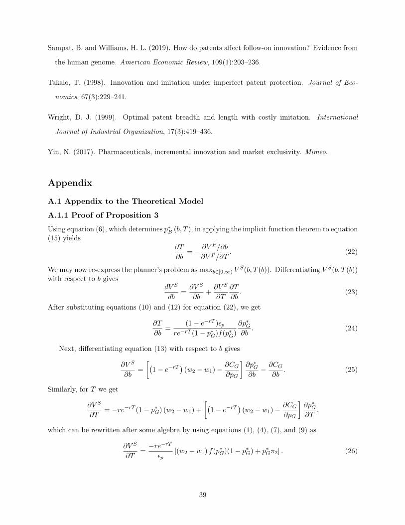
Sampat, B. and Williams, H. L. (2019). How do patents affect follow-on innovation? Evidence from
the human genome. American Economic Review, 109(1):203–236.
Takalo, T. (1998). Innovation and imitation under imperfect patent protection. Journal of Eco-
nomics, 67(3):229–241.
Wright, D. J. (1999). Optimal patent breadth and length with costly imitation. International
Journal of Industrial Organization, 17(3):419–436.
Yin, N. (2017). Pharmaceuticals, incremental innovation and market exclusivity. Mimeo.
Appendix
A.1 Appendix to the Theoretical Model
A.1.1 Proof of Proposition 3
Using equation (6), which determines p∗B (b, T ), in applying the implicit function theorem to equation(15) yields
∂T
∂b= − ∂V
P /∂b
∂V P /∂T. (22)
We may now re-express the planner’s problem as maxb∈[0,∞) VS(b, T (b)). Differentiating V S(b, T (b))
with respect to b givesdV S
db=∂V S
∂b+∂V S
∂T
∂T
∂b. (23)
After substituting equations (10) and (12) for equation (22), we get
∂T
∂b=
(1− e−rT )εpre−rT (1− p∗G)f(p∗G)
∂p∗G∂b
. (24)
Next, differentiating equation (13) with respect to b gives
∂V S
∂b=
[(1− e−rT
)(w2 − w1)−
∂CG∂pG
]∂p∗G∂b− ∂CG
∂b. (25)
Similarly, for T we get
∂V S
∂T= −re−rT (1− p∗G) (w2 − w1) +
[(1− e−rT
)(w2 − w1)−
∂CG∂pG
]∂p∗G∂T
,
which can be rewritten after some algebra by using equations (1), (4), (7), and (9) as
∂V S
∂T=−re−rT
εp[(w2 − w1) f(p∗G)(1− p∗G) + p∗Gπ2] . (26)
39
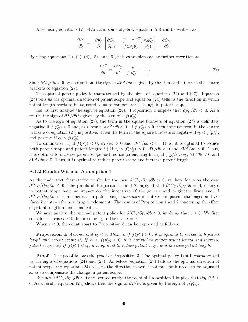
After using equations (24)–(26), and some algebra, equation (23) can be written as
dV S
db= −
∂p∗G∂b
[∂CG∂pG
+
(1− e−rT
)π2p∗G
f(p∗G)(1− p∗G)
]− ∂CG
∂b.
By using equations (1), (2), (4), (8), and (9), this expression can be further rewritten as
dV S
db=∂CG∂b
[εb
f(p∗G)− 1
]. (27)
Since ∂CG/∂b > 0 by assumption, the sign of dV S/db is given by the sign of the term in the squarebrackets of equation (27).
The optimal patent policy is characterized by the signs of equations (24) and (27). Equation(27) tells us the optimal direction of patent scope and equation (24) tells us the direction in whichpatent length needs to be adjusted so as to compensate a change in patent scope.
Let us first analyze the sign of equation (24). Proposition 1 implies that ∂p∗G/∂b < 0. As aresult, the sign of ∂T/∂b is given by the sign of −f(p∗G).
As to the sign of equation (27), the term in the square brackets of equation (27) is definitelynegative if f(p∗G) < 0 and, as a result, dV S/db < 0. If f(p∗G) > 0, then the first term in the squarebrackets of equation (27) is positive. Then the term in the square brackets is negative if εb < f(p∗G),and positive if εb > f(p∗G).
To summarize: i) If f(p∗G) < 0, ∂T/∂b > 0 and dV S/db < 0. Thus, it is optimal to reduceboth patent scope and patent length; ii) If εb > f(p∗G) > 0, ∂T/∂b < 0 and dV S/db > 0. Thus,it is optimal to increase patent scope and reduce patent length; iii) If f(p∗G) > εb, ∂T/∂b < 0 anddV S/db < 0. Thus, it is optimal to reduce patent scope and increase patent length. �
A.1.2 Results Without Assumption 1
As the main text characterize results for the case ∂2CG/∂pG∂b > 0, we here focus on the case∂2CG/∂pG∂b ≤ 0. The proofs of Proposition 1 and 2 imply that if ∂2CG/∂pG∂b = 0, changesin patent scope have no impact on the incentives of the generic and originator firms and, if∂2CG/∂pG∂b < 0, an increase in patent scope increases incentives for patent challenges and re-duces incentives for new drug development. The results of Proposition 1 and 2 concerning the effectof patent length remain unaffected.
We next analyse the optimal patent policy for ∂2CG/∂pG∂b ≤ 0, implying that ε ≤ 0. We firstconsider the case ε < 0, before moving to the case ε = 0.
When ε < 0, the counterpart to Proposition 3 can be expressed as follows:
Proposition 4: Assume that εb < 0. Then, i) if f(p∗G) > 0, it is optimal to reduce both patentlength and patent scope; ii) If εb < f(p∗G) < 0, it is optimal to reduce patent length and increasepatent scope; iii) If f(p∗G) < εb, it is optimal to reduce patent scope and increase patent length.
Proof: The proof follows the proof of Proposition 3. The optimal policy is still characterizedby the signs of equations (24) and (27). As before, equation (27) tells us the optimal direction ofpatent scope and equation (24) tells us the direction in which patent length needs to be adjustedso as to compensate the change in patent scope.
But now ∂2CG/∂pG∂b < 0 and, consequently, the proof of Proposition 1 implies that ∂pG/∂b >0. As a result, equation (24) shows that the sign of ∂T/∂b is given by the sign of f(p∗G).
40
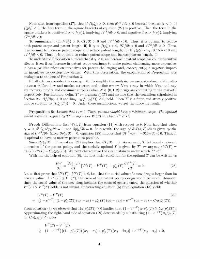
Note next from equation (27), that if f(p∗G) > 0, then dV S/db < 0 because because εb < 0. Iff(p∗G) < 0, the first term in the square brackets of equation (27) is positive. Then the term in thesquare brackets is positive if εb < f(p∗G), implying dV S/db > 0, and negative if εb > f(p∗G), implyingdV S/db < 0.
To summarize: i) If f(p∗G) > 0, ∂T/∂b > 0 and dV S/db < 0. Thus, it is optimal to reduceboth patent scope and patent length; ii) If εb < f(p∗G) < 0, ∂T/∂b < 0 and dV S/db > 0. Thus,it is optimal to increase patent scope and reduce patent length; iii) If f(p∗G) < εb, ∂T/∂b < 0 anddV S/db < 0. Thus, it is optimal to reduce patent scope and increase patent length. �
To understand Proposition 4, recall that if εb < 0, an increase in patent scope has counterintuitiveeffects: Even if an increase in patent scope continues to make patent challenging more expensive,it has a positive effect on incentives for patent challenging and, consequently, a negative impacton incentives to develop new drugs. With this observation, the explanation of Proposition 4 isanalogous to the one of Proposition 3.
Finally, let us consider the case εb = 0. To simplify the analysis, we use a standard relationshipbetween welfare flow and market structure and define wN := NπN + csN in which NπN and csNare industry profits and consumer surplus (when N ∈ {0, 1, 2} drugs are competing in the market),respectively. Furthermore, define T ′ := arg max p∗B(T ) and assume that the conditions stipulated inSection 2.2, ∂f/∂pG < 0 and limT→∞ f(p∗G(T )) < 0, hold. Then T ′ is a finite and strictly positiveunique solution to f(p∗G(T ′)) = 0. Under these assumptions, we get the following result:
Proposition 5: Assume that εb = 0. Then, patents should have a minimum scope. The optimalpatent duration is given by T ∗ := arg maxT W (T ) in which T ∗ < T ′.
Proof: Differentiate first W (b, T ) from equation (14) with respect to b. Note here that whenεb = 0, ∂2CG/∂pG∂b = 0, and ∂p∗B/∂b = 0. As a result, the sign of ∂W (b, T )/∂b is given by thesign of ∂V S/∂b. Since ∂p∗G/∂b = 0, equation (25) implies that ∂V S/∂b = −∂CG/∂b < 0. Thus, itis optimal to have as narrow patents as possible.
Since ∂p∗B/∂b = 0, equation (24) implies that ∂T/∂b = 0. As a result, T is the only relevantdimension of the patent policy, and the socially optimal T is given by T ∗ := arg maxT W (T ) =p∗B (T )V S(T )− CB(p∗B(T )). We next characterize the circumstances under which T ∗ < T.
With the the help of equation (6), the first-order condition for the optimal T can be written as
∂W
∂T=∂p∗B (T )
∂T
[V S(T )− V P (T )
]+ p∗B (T )
∂V S(T )
∂T= 0. (28)
Let us first prove that V S(T )−V P (T ) > 0, i.e., that the social value of a new drug is larger than itsprivate value. If V P (T ) ≥ V S(T ), the issue of the patent policy design would be moot. However,since the social value of the new drug includes the costs of generic entry, the question of whetherV S(T ) > V P (T ) holds is not trivial. Substracting equation (5) from equation (13) yields
V S(T )− V P (T ) (29)=
(1− e−rT
)[(1− p∗G (T )) (w1 − π1) + p∗G (T ) (w2 − π2)] + e−rT (w2 − π2)− CG(p∗G(T )).
From equation (3) we observe that ΠG(p∗G(T )) ≥ 0 implies that(1− e−rT
)π2p∗G (T ) ≥ CG(p∗G(T )).
Approximating the right-hand side of equation (29) downwards by substituting(1− e−rT
)π2p∗G (T )
for CG(pG(T )∗) gives
V S(T )− V P (T )
≥(1− e−rT
)[(1− p∗G (T )) (w1 − π1) + p∗G (T ) (w2 − 2π2)] + e−rT (w2 − π2) > 0,
41

in which the last inequality follows from wN = NπN + csN , N = 1, 2.Next, we evaluate ∂W/∂T at T = T ′. Then, f(p∗G(T ′)) = 0, and equation (26) implies that
∂V S(T ′)/∂T < 0. From the proof of Proposition 2 we also observe that when f(p∗G(T ′)) = 0,∂p∗B(T ′)/∂T = 0. As a result, equation (28) shows that ∂W (T ′)/∂T < 0.
Assume then that i) ∂2W/∂T 2 < 0 for all T so that the problem is well-behaving. Assumefurther that ii) ∂W (0)/∂T > 0. A sufficient condition for ii) is ∂p∗B (0) /∂T > p∗B (0) . To see this,note first from equation (4) that p∗G(0) = 0. Then, when evaluating ∂W/∂T at T = 0 by usingequations (26) and (29) we get
∂W (0)
∂T=∂p∗B (0)
∂T(w2 − π2)− p∗B (0) r (w2 − w1) ,
in which, as indicated by equations, (5), (6), and (11), ∂p∗B (0) /∂T > 0 and p∗B (0) > 0. Clearly,w2 − π2 > r (w2 − w1) .
If both conditions i) and ii) hold, then there exists exactly one solution for equation (28) inthe range where T ∈ (0, T ′) and this solution characterizes the maximum. Note for completeness,that if condition ii) fails to hold, but condition i) holds, then the optimal policy is to set T ∗ = 0.If condition i) fails to hold, then there may be multiple solutions to equation (28). If condition ii)nonetheless holds, there must at least be one local maximum in the range where T ∈ (0, T ′). �
The explanation of Proposition 5 is the following: Since εb = 0, changes in patent scope have noimpact on incentives for new drug development, and an increase in patent scope only increases thecosts of generic firms with no welfare benefits. As a result, it is optimal to have narrow patents.
When changes in patent scope have no impact on incentives for new drug development, patentlength becomes the only relevant patent policy tool. The social planner faces the classic Nordhausianpatent length design problem with the twist that an increase in patent length increases incentivesto challenge new drug patents, creating wasteful costs of patent challenging. Under some plausiblerestrictions on functional forms, the optimal length lies in the range (0, T ′) in which patent lengthhas a positive impact on incentives to develop new drugs and adverse impact on social welfare fora given level of drug development incentives.
Note that the proof of Proposition 5 is based on the assumptions guaranteeing that a finite T ′
solving f(p∗G(T ′) = 0 exists. However, if no such T ′ exists, then Proposition 5 holds trivially sincein that case T ′ →∞.
A.2 Data Construction
In this appendix we describe the details of our data sources and variable construction. We alsoaddress the issue of missing observations in the outcome variable.
A.2.1 FDA Approved Drugs Data: Orange Book and Drugs@FDA
The main data for our empirical analysis comes from the FDA’s publication Approved Drug Productswith Therapeutic Equivalent Evaluations, commonly known as the Orange Book. We use theannual editions 21 – 33 (corresponding years 2001–2013) of the Orange Book. The editions 21 –32 in electronic format were received from the FDA through a Freedom of Information Act (FOIA)request. The 33rd edition was downloaded from the FDA web-pages.7 The Orange Book digitalpublications consist of product, patent, and exclusivity data files. The product file identifies eachdrug with an FDA application number and, among others, lists information on active ingredient,
7The latest release of the Orange Book is available at: https://www.fda.gov/Drugs/InformationOnDrugs/ucm129662.htm, last accessed on April 18, 2020.
42

dosage form, strength, producer, trade name and approval date. The patent file lists the patentsincluded in each drug application. If a drug is covered by the FDA exclusivity the type of exclusivityand its latest expiration date are listed in the exclusivity file. Using the drug application numberswe first link the Orange Book data files into one, and then link it with the early 2014 release of theDrugs@FDA database, Application and Product Tabs.8
The unit of observation in our analysis is a new drug patent. By definition, only new medicines,so called New Drug Applications (NDAs), may be listed in the Orange Book with correspondingpatent information. Each patent thus protects an NDA. To account for the characteristics of NDAs,we aggregate drug application level data into the patent level observations. For example, if a patentprotects a drug in a tablet form, we assign value one to the patent level indicator variable Tablet.The indicator variables for two other common drug forms, Capsule and Injectable, are calculatedsimilarly. Some patents protect several active ingredients listed in the Orange Book. So we identifythe first FDA-approved active ingredient protected by a given patent. We also identify the firstFDA approval date of an NDA protected by a patent.
New chemical exclusivity is marked in the Orange Book by the code "NCE", and orphan drugexclusivity by the code "ODE", signifying a drug intended to treat rare conditions affecting lessthan 200,000 individuals in the US (21 U.S.C. § 360bb(2)). Using these codes, we construct theindicator variables New chemical exclusivity and Orphan drug exclusivity measuring whether or nota patent protects a drug with new chemical or orphan drug exclusivity.
A drug receives pediatric exclusivity if its producer has conducted clinical trials and proved thesafety and efficacy of its drug for children. In this case, additional six month of exclusive marketingrights are added to all existing patents and exclusivities covering the drug (21 U.S.C. § 355a(b)). Apatent listed for an application with pediatric exclusivity has is recorded twice in the Orange Book:first, with the original patent number and its corresponding expiration date, and second, with theoriginal patent number followed by a *PED" mark and a new expiration date six months later thanthe original expiration date. Based on "*PED" designations, we assign value one to the indicatorvariable Pediatric exclusivity if the patent protects a drug with pediatric exclusivity. Using theOrange Book, we also compute the latest FDA exclusivity year for each patent, and identify thepatent expiration date.
We identify priority reviewed drugs from the Drugs@FDA database. Priority reviewed drugsare assessed by the FDA faster as they, if approved, would represent significant improvements overavailable therapy, and thus might be particularly valuable. During our data period, such drugs weremarked by a letter "P" or "P*" in the Therapeutic Potential column of the Drugs@FDA ApplicationTab. Based on these codes, we construct the indicator variable Priority measuring whether or nota patent protects a drug that was priority reviewed by the FDA.
A.2.2 Measuring Patent Challenges: FDA ANDA Approval Letters and Orange Book
We measure generic entry via successful PIV challenges to new drug patents. In a PIV challenge,a generic firm seeks to enter prior to the expiration of a new drug patent by filing an AbbreviatedNew Drug Application (ANDA) to the FDA containing a certification that the new drug patent isinvalid or noninfringed by the generic drug (21 U.S.C. § 355(j)(2)(A)(vii)(IV)). To construct theoutcome variable, we first obtain the list of the approved ANDAs containing PIV certifications fromthe FDA through a FOIA request. To link this list with patent numbers, we seek the FDA’s lettersapproving these ANDAs. Each originator drug is usually protected by multiple patents, and theseapproval letters specify all originator drug patents that have successfully been challenged. Some of
8The latest release of Drugs@FDA is available at: https://www.fda.gov/Drugs/InformationOnDrugs/ucm079750.htm, last accessed on April 2, 2020.
43

the letters are readily available from the FDA web-pages through the Drugs@FDA search engine.To collect more letters, we submit FOIA requests to the FDA. The data collection process has beenslow, since the FDA only accepts a few FOIAs per month.
We read each approval letter and record patent numbers together with corresponding PIV cer-tifications mentioned in the letters. Using patent numbers, we then link the data on PIV challengesfrom ANDA approval letters to the data on all new drug patents listed in the Orange Book. Somepatents are challenged by multiple generics, so we calculate the earliest PIV ANDA approval datefor each patent from the Orange Book files. We then construct our outcome variable, PIV entry,as an indicator which equals one if a new drug patent has successfully been challenged via PIVcertification at least once.
PIV challenges by definition only concern patents before they expire. However, six patents in oursample are listed in the FDA approval letters as challenged through PIV certification even thoughthe patents expired before the approval of the first generic drug. For consistency, we classify themas non-challenged, but the results do not significantly change if we assign them as challenged.
Missing Observations in PIV Challenged Patent Numbers. Some of the PIV challengedpatent numbers are missing from our dataset. The FDA provided us with a list of 1020 ANDAscontaining PIV certifications and we have collected the 677 approval letters for these ANDAs. Thereare thus 343 ANDAs in our sample for which the exact numbers of challenged patents are missing.
While we continue to file the FOIA requests to the FDA so as to update the data, we believethat our estimation sample is comprehensive enough to allow for an accurate measurement of bothour outcome variable, PIV entry, and its timing: First, to measure PIV entry correctly, we only haveto observe one of potentially many successful challenges of a new drug patent. Second, we aggregatethe challenges to the active ingredient level, and measure whether or not we observe both 180-daygeneric exclusivity and a PIV challenged patent for each challenged active ingredient. That 180-dayexclusivity is granted to the first filer of an ANDA and reliably measures the first successful PIVchallenge of an active ingredient. ANDAs which have received 180-day exclusivity are marked by"PC" designation in the Orange Book. Our sample includes 1009 unique active ingredients and 150of them are associated with ANDAs holding 180-day exclusivity. Out of those 150 active ingredients,we fail to observe a PIV challenged patent number only in 13 cases. Third, when looking at those150 PIV challenged active ingredients, the average year of the first PIV entry is in practice the sameregardless of whether we calculate it based on the earliest approval date of generic drugs with 180-day exclusivity or based on the earliest approval date of generic drugs with non-missing challengedpatent numbers. This evidence suggests that we also measure the timing of (the first) PIV entryreliably. Fourth, when filing the FOIA requests to the FDA in stages, we have randomized overthe target ANDA approval letters. As a result, each month we receive approval letters of severalrandomly chosen ANDAs and add the challenged patent numbers from these letters to our sample.For some time now, our outcome variable of interest, PIV entry, has remained virtually unchangedas we add missing patent numbers.
A.2.3 Measuring Effective Patent Length, Grant Lags, PTAs, and Some Patent Char-acteristics: USPTO PatEx and Orange Book
Effective Patent Length. Our primary measure of the effective length of patent i is
Effective lengthi = Expiration datei −max{Grant datei,Drug approval datei},
in which Expiration datei is the date when patent i expired, Drug approval datei is the date whenthe FDA approved the first of potentially many new drugs protected by patent i, and Grant dateiis the date when the USPTO issued patent i. We identify patent grant dates from the Application
44
Data Tab of the USPTO PatEx, and the FDA approval and patent expiration dates from theproduct and patent files, respectively, of the Orange Book.
Patent Grant Lags. We calculate the grant lag of patent i simply as
Grant lagi = Grant datei − Filing datei,
in which Filing datei is the date on which USPTO received the application that was subsequentlyissued as patent i. Like grant dates, we identify patent filing dates and application numbers fromthe Application Data Tab of PatEx.
PTAs. We use patent application numbers to collect PTAs from the Patent Term AdjustmentTab of PatEx. Compensations for patent term forgone due to the USPTO regulatory delays arelabeled as patent term extensions for patents filed after the adoption of TRIPS on June 8, 1995 butbefore the implementation of AIPA, on May 29, 2000, after which the compensations are labeled aspatent term adjustments.9 For brevity and following the variable label in the PatEx files, we callboth of these term modifications PTAs.
Other Patent Characteristics from PatEx. We assign the value one to the indicatorvariable Continuing patenti if patent i has been filed as a continuation, a continuation-in-part or adivisional application. We identify this information using application numbers from the ContinuityData Tab of PatEx where continuation, continuation-in-part and divisional applications are recordedas "CON", "CIP" and "DIV", respectively.
We use the Application Data Tab of PatEx to retrieve the USPC numbers and patent examiners’Art Unit codes. We identify the Technology Centers from the first two digits of the Art Unit codes.As the number of patents and their examiners in some Technology Centers is relatively small, wecombine patents prosecuted in the Technology Centers that have issued less than 100 new drugpatents into one group (with 188 patents).
A.2.4 Measuring Claim Scope: USPTO Patent Claims Research Dataset
Our measures of patent claim scope are the count of words, the counts of Markush groups andconjunctions "or" in the first independent claim, and the count of independent claims in eachpatent. The data on these measures of claim scope is available from the USPTO Patent ClaimsResearch Dataset and we link it to our main dataset using patent numbers.
We instrument these measures of claim scope with the "examiner’s historical average" calculatedaccording to equation (20). To construct the instruments, we first identify the examiners of new drugpatents from the Application Tab of PatEx. We then find all patents reviewed by these examinersand link the data using the patent number to the USPTO Patent Claims Research Dataset. Finally,we identify the scope outcomes for all granted patents reviewed by these examiners.
A.2.5 Measuring Method and Active Ingredient Patents: Google Patent
We combine text recognition algorithms and manual verification to identify method and activeingredient patents. Our classification approach employs the texts of the abstracts and first claimsof patents. We collected the full texts of patent abstracts and the first claims using Google PatentSearch Engine and data scrapping algorithms (written in Python using BeautifulSoup and urlib2packages.)
Method patents covering drugs mostly pertain to the method of use of a drug or the ulti-mate intended effect of a patented chemical. Typically the first claim of a method patent begins
9See, e.g., https://www.uspto.gov/web/offices/pac/mpep/s2720.html and https://www.uspto.gov/web/offices/pac/mpep/s2730.html, last accessed on April 3, 2020.
45

with a word "method" or "process". For example, the first claim of the USPTO patent number4870105 begins with: "A method for inhibiting gastrointestinal absorption ...". Hence, we assignthe Method patenti dummy equal to one, if the text of the first claim of a patent begins with thewords "method" or "process". We manually verified texts of multiple patents to ensure the accuracyof the assignment.
We assign the value one to the Active ingredienti dummy if the first claim of a patent per-tains a chemical formula. We classify the first claim as a chemical formula when its first foursymbols are a combination of single letters, dashes, commas or digits, for example, "N,N" or "R-R". Active ingredienti also equals one if the first three words of the first claim indicate a chemicalcompound and its variations. Word combinations used in chemical compound patents are, e.g.,"composition of matter", "compound", "chemical compound", "antiviral compound", "amine", and"peptide". We also identify patents claiming solid forms (crystallines) of compounds, derivativesof compounds, and some other cases based as active ingredient patents. (In identifying the activeingredient patents, we used Python package re and heavily relied on regular expressions.)
Manual checks suggest that most of the patents in our sample which our approach does notclassify as methods nor active ingredients pertain to drug delivery systems, devices, or formulations.
A.2.6 Measuring Backward and Forward Citations: USPTO PatFT
We collect the data on forward and backward citations from PatFT using a Python algorithm.We define the variable Backward citationsi as the total number of patent documents (includingforeign) listed on under the headline "References Cited" of patent i in our sample, and the variableForward citationsi as the number of the US issued patents mentioning patent i in their "ReferencesCited" list. Forward citation data was collected from PatFT using "Referenced By" retrieval toolin October 2017.
A.2.7 Measuring Patent Family: EPO Open Patent Services
Various definitions of the patent family size are used in the literature. One commonly used definitionof the patent family size (see, e.g., Lanjouw and Schankerman, 2004; Sampat and Williams, 2019)is the number of distinct countries where the same invention has been patented. We follow thisdefinition and construct the variable Patent family sizei as follows: We first collect the "DOCDBsimple patent families" of the new drug patents in our sample from the Open Patent Servicesof the EPO in October 2017 10. To collect the data, we used an algorithm and the ApplicationProgramming Interface granted to authors by the EPO. (The algorithm is written in Python usingepo_ops and xml packages).
A "DOCDB simple patent family" may contain multiple patents from one patent office sinceit, e.g., includes continuing patents in addition to their parent patents. To solve the problem, wecount the unique countries based on the country codes, which are the two letters preceding patentnumbers retrievable from the Open Patent Services (e.g., Canadian patents contain a prefix CA,Japanese JP, Finnish FI, etc.). Thus, even if the DOCDB simple patent family lists several patentswith the country code JP, we count Japan in our family size variable only once.
10https://www.epo.org/searching-for-patents/helpful-resources/first-time-here/patent-families/docdb.html, lastaccessed on April 24, 2020
46

A.3 Patent Length Estimations: Robustness
A.3.1 Other Impacts of TRIPS and AIPA
Besides the changes affecting the effective patent length described in Section 5.1, TRIPS and AIPAintroduced other changes to the U.S. patent law. In what we analyze some of these other changesthat could threaten our identification of the effects of the effective patent length on PIV entry, affectthe interpretation of our results, or be used to further support our main results.
Provisional Patent Applications. Another major change associated with the implementationof TRIPS was the introduction of a provisional patent application as a simplified version of a regularutility patent application. Provisional applications include no claims nor description of prior art,are not subject to examination, and automatically expire after one year (35 U.S.C. § 111 (b)). Thepurpose of a provisional application is to give priority rights on invention without starting the patentclock: If a regular utility patent application is filed for the same invention before the expiration ofits provisional application, the priority date is the provisional application date but the patent termis calculated from the utility patent application date.
A threat to our identification might arise if the use of provisional applications varies acrosspatents depending on their prosecution time. To address this concern, we first create the indicatorProvisional applicationi which equals one if patent i claims the priority date of a provisional appli-cation. We identify these patents based on the "PRO" designations listed in the Continuity DataTab of PatEx. We then estimate the DiD model of equation (19) using the Provisional applicationiindicator as the dependent variable.
The results reported in column (1) of Table 6 suggest that the introduction of provisionalapplications is unlikely to drive our results: we observe no systematic relationship between theprobability of a patent claiming the priority date of a provisional application and its prosecutiontime in the different policy regimes. This conclusion is confirmed by another robustness check: whenwe estimate equation (19) using a sample that excludes all patents with Provisional applicationi = 1,the effects of TRIPS and AIPA, reported in column (1) of Table 7 in the next subsection, become,if anything, stronger and more precisely estimated than in Table 3.
47

Table 6: Patent Law Changes and Patent Characteristics by Patent Grant Lag.
Outcome Provi- Conti- log(Markush Active log(Public log(Family log(Backwardsional nuing groups+1) ingredient length) size) citations+1)(1) (2) (3) (4) (5) (6) (7)
Grant lag ≥3 years 0.000 0.076** 0.030 0.001 -0.081*** -0.174* 0.385***(0.000) (0.030) (0.038) (0.033) (0.013) (0.091) (0.078)
Grant lag ≥3 years,Post-TRIPS 0.024 -0.138** -0.032 -0.012 -0.088*** 0.013 0.140
(0.030) (0.055) (0.054) (0.041) (0.023) (0.141) (0.123)Grant lag ≥3 years,Post-AIPA 0.019 -0.193*** -0.036 -0.063* 0.294*** 0.216 -0.078
(0.045) (0.052) (0.058) (0.037) (0.026) (0.140) (0.133)Mean dep. variable 0.214 0.589 0.247 0.226 2.777 1.905 2.760Observations 3517 3517 3485 3517 3517 3511 3517Filing year FE × × × × × × ×
Notes: This table reports estimates of the effects of TRIPS and AIPA on various patent characteristics. Columns(1)–(7) show coefficients from an OLS regression of the Provisional application indicator, the Continuing patent indi-cator, log(Markush groups+1), the Active ingredient patent indicator, log(Public length), log(Patent family size), andlog(Backward citations+1), respectively, on three different indicators for patents with at least a three-year grant lag andfiling year fixed effects (FEs). Standard errors, in parentheses, are clustered at the level of patents protecting the sameactive ingredient. ∗ p < 0.10, ∗∗ p < 0.05, ∗∗∗ p < 0.01.
Continuing Patents. In the case of continuing patents – which represent close to 60 percentof our sample (see Table 1) – TRIPS had an impact on the effective patent length besides thoseeffects discussed in Section 5.1. Before TRIPS, the terms of continuing patents and other patentswere calculated in the same way, implying that continuing patents typically expired later thantheir (earlier-filed) parent patents. After TRIPS, continuing patents expire simultaneously withtheir parent patent (35 U.S.C. §154 (a)(2)). Thus, TRIPS shortened the effective patent length ofcontinuing patents more than that of other patents, and this shortening is stronger for continuingpatents prosecuted over three years. As a result, long patent prosecution times might incentivizeoriginator firms to opt for separate patent applications instead of continuing applications afterTRIPS. Supporting this idea, patents with long prosecution lags are less likely to be continuingafter TRIPS, compared to other patents in our sample, as shown in column (2) of Table 6.
A smaller share of continuing patents in the post-TRIPS period of our sample has severalimplications: First, it implies a stronger variation in the effective patent length stemming from thevariation in patent grant lags. Second, since continuing patent applications might be used as a toolto make patent protection stronger (see, e.g., Lemley and Moore 2004), it raises the concern thatour baseline estimates of the effect of TRIPS on patents with long prosecution lags would partiallyreflect narrower patent protection. To address this concern, we estimate the DiD model of equation(19) using a sample of continuing patents. The results, reported in column (2) of Table 7, supportour main result of the positive impact of longer effective patent length on the probability of PIVentry: the effects of TRIPS and AIPA on the patents prosecuted at least three years are strongerthan in any other specification. The results in columns (3) (4), and (7), discussed at the end of thesubsection, also mitigate the concern that potentially narrower patent protection in the post-TRIPSperiod would be driving our main results.
Third, taken together, the results in columns (2) of Table 6 and Table 7 suggest that TRIPS madecontinuing patents with long grant lags less valuable for originator firms even if it simultaneously
48
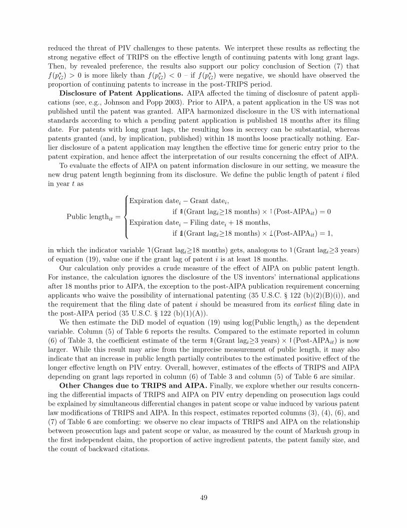
reduced the threat of PIV challenges to these patents. We interpret these results as reflecting thestrong negative effect of TRIPS on the effective length of continuing patents with long grant lags.Then, by revealed preference, the results also support our policy conclusion of Section (7) thatf(p∗G) > 0 is more likely than f(p∗G) < 0 – if f(p∗G) were negative, we should have observed theproportion of continuing patents to increase in the post-TRIPS period.
Disclosure of Patent Applications. AIPA affected the timing of disclosure of patent appli-cations (see, e.g., Johnson and Popp 2003). Prior to AIPA, a patent application in the US was notpublished until the patent was granted. AIPA harmonized disclosure in the US with internationalstandards according to which a pending patent application is published 18 months after its filingdate. For patents with long grant lags, the resulting loss in secrecy can be substantial, whereaspatents granted (and, by implication, published) within 18 months loose practically nothing. Ear-lier disclosure of a patent application may lengthen the effective time for generic entry prior to thepatent expiration, and hence affect the interpretation of our results concerning the effect of AIPA.
To evaluate the effects of AIPA on patent information disclosure in our setting, we measure thenew drug patent length beginning from its disclosure. We define the public length of patent i filedin year t as
Public lengthit =
Expiration datei −Grant datei,
if 1(Grant lagi≥18 months)× 1(Post-AIPAit) = 0
Expiration datei − Filing datei + 18 months,if 1(Grant lagi≥18 months)× 1(Post-AIPAit) = 1,
in which the indicator variable 1(Grant lagi≥18 months) gets, analogous to 1(Grant lagi≥3 years)of equation (19), value one if the grant lag of patent i is at least 18 months.
Our calculation only provides a crude measure of the effect of AIPA on public patent length.For instance, the calculation ignores the disclosure of the US inventors’ international applicationsafter 18 months prior to AIPA, the exception to the post-AIPA publication requirement concerningapplicants who waive the possibility of international patenting (35 U.S.C. § 122 (b)(2)(B)(i)), andthe requirement that the filing date of patent i should be measured from its earliest filing date inthe post-AIPA period (35 U.S.C. § 122 (b)(1)(A)).
We then estimate the DiD model of equation (19) using log(Public lengthi) as the dependentvariable. Column (5) of Table 6 reports the results. Compared to the estimate reported in column(6) of Table 3, the coefficient estimate of the term 1(Grant lagi≥3 years)× 1(Post-AIPAit) is nowlarger. While this result may arise from the imprecise measurement of public length, it may alsoindicate that an increase in public length partially contributes to the estimated positive effect of thelonger effective length on PIV entry. Overall, however, estimates of the effects of TRIPS and AIPAdepending on grant lags reported in column (6) of Table 3 and column (5) of Table 6 are similar.
Other Changes due to TRIPS and AIPA. Finally, we explore whether our results concern-ing the differential impacts of TRIPS and AIPA on PIV entry depending on prosecution lags couldbe explained by simultaneous differential changes in patent scope or value induced by various patentlaw modifications of TRIPS and AIPA. In this respect, estimates reported columns (3), (4), (6), and(7) of Table 6 are comforting: we observe no clear impacts of TRIPS and AIPA on the relationshipbetween prosecution lags and patent scope or value, as measured by the count of Markush group inthe first independent claim, the proportion of active ingredient patents, the patent family size, andthe count of backward citations.
49

A.3.2 Other Subsamples and Specifications
In Table 7, we provide further evidence that our results from the estimation of the DiD modelof equation (19) are robust to using different subsamples and specifications. As discussed in theprevious subsection, columns (1) and (2) report estimates using sample that only include patentswhich do not claim the priority date of a provisional application and continuing patents, respectively.
We study robustness to excluding related new drug patents. We identify all our sample patentssharing the same parent patent application using information on parent applications from the Con-tinuity Data Tab of PatEx. The results in column (3) are generated by a sample that excludes allother new drug patents sharing the common parent application except for the latest one.
In column (4) the results arise from a sample that only includes patents for which we observeFDA exclusivity. These patents might be more valuable or – as our results of Table (2) indicate– more difficult to challenge than patents for which we observe no FDA exclusivity. Column (5)reports estimates from a model that, analogous to survival models, includes fixed effects to controlfor the length of exposure of a patent to PIV challenges. In this specification we, in addition to afull set of other controls, include a dummy measuring the time (in years) between the grant dateof a patent and the earliest successful PIV patent challenge date or, in the absence of successfulPIV challenges, the patent expiration date. Finally, we estimate a model that extends our baselinespecification to allows for richer interactions between grant lags and patent policy reforms, andreport the results in column (6).
The signs and magnitudes of the coefficient estimates reported in Table 7 are similar to thosecoefficients reported in columns (1)–(5) of Table 3. If anything, the effects of TRIPS and AIPAare now stronger and more precisely estimated. Coefficients of the additional interaction termsinvolving patents with a grant lag exceeding five years reported in Column (6) are impreciselyestimated, possibly because we have only 417 such patents in our sample.
50
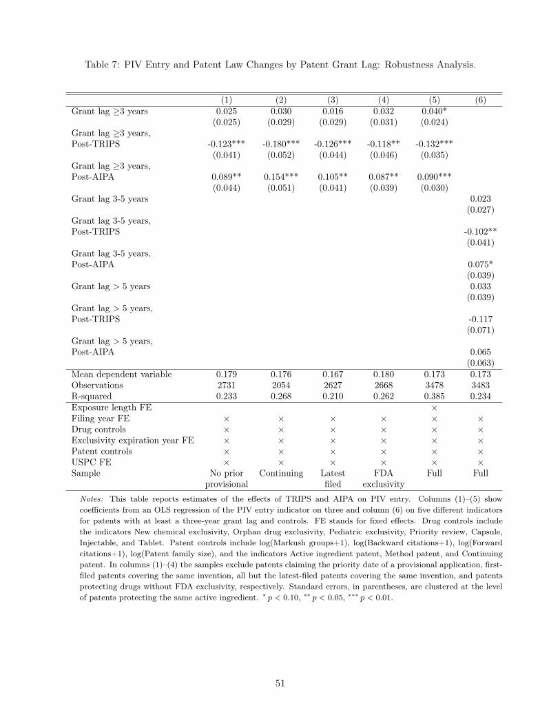
Table 7: PIV Entry and Patent Law Changes by Patent Grant Lag: Robustness Analysis.
(1) (2) (3) (4) (5) (6)Grant lag ≥3 years 0.025 0.030 0.016 0.032 0.040*
(0.025) (0.029) (0.029) (0.031) (0.024)Grant lag ≥3 years,Post-TRIPS -0.123*** -0.180*** -0.126*** -0.118** -0.132***
(0.041) (0.052) (0.044) (0.046) (0.035)Grant lag ≥3 years,Post-AIPA 0.089** 0.154*** 0.105** 0.087** 0.090***
(0.044) (0.051) (0.041) (0.039) (0.030)Grant lag 3-5 years 0.023
(0.027)Grant lag 3-5 years,Post-TRIPS -0.102**
(0.041)Grant lag 3-5 years,Post-AIPA 0.075*
(0.039)Grant lag > 5 years 0.033
(0.039)Grant lag > 5 years,Post-TRIPS -0.117
(0.071)Grant lag > 5 years,Post-AIPA 0.065
(0.063)Mean dependent variable 0.179 0.176 0.167 0.180 0.173 0.173Observations 2731 2054 2627 2668 3478 3483R-squared 0.233 0.268 0.210 0.262 0.385 0.234Exposure length FE ×Filing year FE × × × × × ×Drug controls × × × × × ×Exclusivity expiration year FE × × × × × ×Patent controls × × × × × ×USPC FE × × × × × ×Sample No prior Continuing Latest FDA Full Full
provisional filed exclusivity
Notes: This table reports estimates of the effects of TRIPS and AIPA on PIV entry. Columns (1)–(5) showcoefficients from an OLS regression of the PIV entry indicator on three and column (6) on five different indicatorsfor patents with at least a three-year grant lag and controls. FE stands for fixed effects. Drug controls includethe indicators New chemical exclusivity, Orphan drug exclusivity, Pediatric exclusivity, Priority review, Capsule,Injectable, and Tablet. Patent controls include log(Markush groups+1), log(Backward citations+1), log(Forwardcitations+1), log(Patent family size), and the indicators Active ingredient patent, Method patent, and Continuingpatent. In columns (1)–(4) the samples exclude patents claiming the priority date of a provisional application, first-filed patents covering the same invention, all but the latest-filed patents covering the same invention, and patentsprotecting drugs without FDA exclusivity, respectively. Standard errors, in parentheses, are clustered at the levelof patents protecting the same active ingredient. ∗ p < 0.10, ∗∗ p < 0.05, ∗∗∗ p < 0.01.
51

A.4 Patent Scope Estimations: Robustness
In this section we explore the robustness of our patent claim scope estimates. Table 8 reportsestimates of various claim scope measures from the OLS model of equation (18). Column (1) showsan estimate using the specification of column (3) in Table (2). We then replace the count of Markushgroups in the first independent claim with alternative measures of patent claim scope: the countof the conjunction "or" in the first independent claim (column (2)), the count of words in the firstindependent claim (column (3)), the count of independent claims (column (4)). The coefficientestimate in colunm (3) suggests a statistically significant but small negative relationship betweenPIV entry and patent scope, as measure by the count of the conjunction "or" in the first independentclaim. When compared with our IV estimates from Table (5), there appears to be an upward biasin most of these OLS estimates.
Tables (9)–(11) report the results from our exploration of the robustness of 2SLS estimatesof patent scope measures. Tables (9) and (10) show that the results reported in Table (5) arerobust, respectively, to the exclusion of control variables, and to the inclusion of the interactionof Technology Center fixed effects with filing year fixed effects, to control for Technology Centerspecific trends. Table (11) reports estimates from a regression in which we replace TechnologyCenter fixed effects with Art Unit fixed effects. The number of patents per Art Unit is small, only21 on average. Even if we group Art Units with less than 10 patents into one group of 266 patents,coefficients of the scope measures become less precisely estimated (although remaining similar inmagnitude) than in Table (5). The only scope measure generating statistically significant effects isthe count of words in the first independent claim, as shown by column (3) of Table (11)
We have also verified that our results are robust to using the following alternative measures ofclaim scope: the count of claims, and the counts of characters and the phrase "consisting of" in thefirst independent claim. We omit the regressions using these measures for brevity.
52

Table 8: PIV Entry and Patent Scope: OLS Estimates.
(1) (2) (3) (4)log(Markush groups+1) -0.013
(0.012)log(Conjunctions "or"+1) -0.020***
(0.007)log(Words) -0.001
(0.007)log(Independent claims) -0.009
(0.008)Mean dependent variable 0.173 0.173 0.173 0.173Observations 3483 3483 3483 3485R-squared 0.242 0.241 0.243 0.241Technology Center FE × × × ×Filing year FE × × × ×Drug controls × × × ×Exclusivity expiry year FE × × × ×Patent controls × × × ×USPC FE × × × ×
Notes: This table reports coefficients from OLS regressions of the PIVentry indicator on measures of claim scope and controls. FE stands forfixed effects. Drug controls include the indicators New chemical exclusiv-ity, Orphan drug exclusivity, Pediatric exclusivity, Priority review, Cap-sule, Injectable, and Tablet. Patent controls include log(Effective length),log(Backward citations+1), log(Forward citations+1), log(Patent familysize), and the indicators Active ingredient patent, Method patent, andContinuing patent. Standard errors, in parentheses, are clustered atthe level of patents protecting the same active ingredient. ∗ p < 0.10,∗∗ p < 0.05, ∗∗∗ p < 0.01.
53

Table 9: PIV Entry and Patent Scope:Robustness of IV Estimates to Exclusion of Control Variables.
(1) (2) (3) (4)log(Markush groups+1) -0.244***
(0.071)log(Conjunctions "or"+1) -0.095***
(0.030)log(Words) -0.484**
(0.233)log(Independent claims) -0.154
(0.123)Mean dependent variable 0.173 0.173 0.173 0.173Observations 3447 3447 3447 3449First-stage F-statistic 41.446 127.960 5.417 15.264Technology Center FE × × × ×Filing year FE × × × ×USPC FE × × × ×
Notes: This table reports coefficients from 2SLS regressions of the PIV en-try indicator on instrumented measures of claim scope and controls. Theinstruments are the cumulative averages of the scope measures of all patentsreviewed by the examiner of a new drug patent, until one year precedingthe filing year of the new drug patent. The first stage F-statistic tests ison the excluded instruments. FE stands for fixed effects, respectively. Ro-bust standard errors are reported in parentheses. ∗ p < 0.10, ∗∗ p < 0.05,∗∗∗ p < 0.01.
54

Table 10: PIV Entry and Patent Scope:Robustness of IV Estimates to Technology Center Specific Trends.
(1) (2) (3) (4)log(Markush groups+1) -0.218**
(0.091)log(Conjunctions "or"+1) -0.101*
(0.052)log(Words) -0.219**
(0.091)log(Independent claims) 0.062
(0.132)Mean dependent variable 0.173 0.173 0.173 0.173Observations 3445 3445 3445 3447First-stage F-statistic 24.520 43.897 14.769 10.592Technology Center FE × Filing year FE × × × ×Drug controls × × × ×Exclusivity expiry year FE × × × ×Patent controls × × × ×USPC FE × × × ×
Notes: This table reports coefficients from 2SLS regressions of the PIV entry indicator oninstrumented measures of claim scope and controls. The instruments are the cumulativeaverages of the scope measures of all patents reviewed by the examiner of a new drugpatent, until one year preceding the filing year of the new drug patent. The first stageF-statistic tests is on the excluded instruments. FE stands for fixed effects. Drug con-trols include the indicators New chemical exclusivity, Orphan drug exclusivity, Pediatricexclusivity, Priority review, Capsule, Injectable, and Tablet. Patent controls includelog(Effective length), log(Backward citations+1), log(Forward citations+1), log(Patentfamily size), and the indicators Active ingredient patent, Method patent, and Continuingpatent. Robust standard errors in parentheses. ∗ p < 0.10, ∗∗ p < 0.05, ∗∗∗ p < 0.01.
55
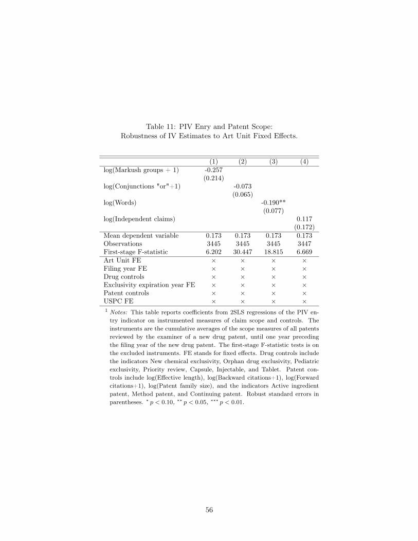
Table 11: PIV Enry and Patent Scope:Robustness of IV Estimates to Art Unit Fixed Effects.
(1) (2) (3) (4)log(Markush groups + 1) -0.257
(0.214)log(Conjunctions "or"+1) -0.073
(0.065)log(Words) -0.190**
(0.077)log(Independent claims) 0.117
(0.172)Mean dependent variable 0.173 0.173 0.173 0.173Observations 3445 3445 3445 3447First-stage F-statistic 6.202 30.447 18.815 6.669Art Unit FE × × × ×Filing year FE × × × ×Drug controls × × × ×Exclusivity expiration year FE × × × ×Patent controls × × × ×USPC FE × × × ×1 Notes: This table reports coefficients from 2SLS regressions of the PIV en-try indicator on instrumented measures of claim scope and controls. Theinstruments are the cumulative averages of the scope measures of all patentsreviewed by the examiner of a new drug patent, until one year precedingthe filing year of the new drug patent. The first-stage F-statistic tests is onthe excluded instruments. FE stands for fixed effects. Drug controls includethe indicators New chemical exclusivity, Orphan drug exclusivity, Pediatricexclusivity, Priority review, Capsule, Injectable, and Tablet. Patent con-trols include log(Effective length), log(Backward citations+1), log(Forwardcitations+1), log(Patent family size), and the indicators Active ingredientpatent, Method patent, and Continuing patent. Robust standard errors inparentheses. ∗ p < 0.10, ∗∗ p < 0.05, ∗∗∗ p < 0.01.
56

A.5 Elasticity Calculations for Section 7
Recall from Section 7 the definitions
ξj :=∂pG∂j
j
pG, j ∈ {b, T} . (30)
We now prove the claims of Section 7 concerning the relation of ξj to εp of equation (1), and to εbof equation (2).
Let us start with the relationship between ξT and εp. Using the first-order condition (4) toeliminate π2 from equation (7) allows us to rewrite equation (7) as
∂p∗G∂T
=re−rT
(1− e−rT )
∂CG/∂pG∂2CG/∂p2G
.
Multiplying both sides of this equation by T/p∗G gives
∂p∗G∂T
T
p∗G=
e−rT rT
(1− e−rT )
∂CG/∂pGp∗G∂
2CG/∂p2G.
By using the definitions of the elasticities (1) and (30) this equation can be rewritten as
ξT =e−rT rT
(1− e−rT )εp,
i.e.,
εp =e−rT rT
(1− e−rT )ξT.
This equation equals equation (21) of Section 7.To link ξb with εp, we assume the functional form of the generic firm’s cost function specified
by equation (16), and further stipulate that c(b) = cb. Then, equation (16) can be expressed as
CG(pG, b) =cbpηGGηG
. (31)
Using equation (31) in equation (4) yields after some algebra
p∗G (b, T ) =
[(1− e−rT
)π2
cb
] 1ηG−1
. (32)
Differentiating equation (32) with respect to b gives
∂p∗G∂b
= −1
b
(1
ηG − 1
)[(1− e−rT
)π2
cb
] 1ηG−1
.
Using equation (32) and multiplying both sides of the equation above by b/p∗G gives
∂p∗Gdb
b
p∗G=
1
1− ηG,
57

which may be rewritten by using equation (30) as
ηG = 1− 1
ξb. (33)
Using equation (16) in equation (1) implies that εp = ηG − 1 which, according to equation (33),is equivalent to εp = −1/ξb, as claimed in Section 7.
Finally, our claim in Section (7) that εb = 1− 1/ξb directly follows from equation (33) and fromExample 1 of Section 2 where we show that εb = ηG.
58