Optimal Paths in Dynamic Networks

with Dependent Random Link Travel Times

He HuangSingapore-MIT Alliance for Research and TechnologyFuture Urban MobilityS16-04-193 Science Drive 2Singapore 117543Phone: +65-6601-1636Email: huanghe@smart.mit.edu

Song GaoDepartment of Civil and Environmental EngineeringUniversity of Massachusetts Amherst214C Marston Hall130 Natural Resources RoadAmherst, MA 01003Phone: +1-413-545-2688Fax: +1-413-545-9569Email: sgao@engin.umass.edu

1

Abstract

This paper addresses the problem of finding optimal paths in a net-work where all link travel times are stochastic and time-dependent,and correlated over time and space. A disutility function of traveltime is defined to evaluate the paths, and those with the minimumexpected disutility are defined as the optimal paths. Bellman’s Prin-ciple (Bellman, 1958) is shown to be invalid if the optimality or non-dominance of a path and its sub-paths is defined with respect to thecomplete set of departure times and joint realizations of link traveltime. An exact label-correcting algorithm is designed to find optimalpaths based on a new property for which Bellman’s Principle holds.The algorithm has exponential worst-case computational complexity.Computational tests are conducted on three types of networks. Al-though the average running time is exponential, the number of theoptimal path candidates is polynomial on two networks and growsexponentially in the third one. Computational results in large net-works and analytical results in a small network show that stochasticdependencies affect optimal path finding in a stochastic network, andthat the impact is closely related to the levels of correlation and riskattitude.

Keywords Optimal path; Non-dominated path; Correlation; Stochas-tic dependency; Risk aversion

2

1 Introduction

Traffic networks are inherently uncertain. Random disruptions like crashes,vehicle breakdown, bad weather, construction and maintenance activitiesgreatly affect the reliability of transportation systems and account for morethan half of the congestion in the United States’ 439 urban areas (Schrankand Lomax, 2009). In order to model travelers’ route choice decisions ina transportation system, a stochastic time-dependent (STD) network is re-quired to capture such uncertainties, where link travel times are time-dependentrandom variables.

Strong dependencies exist among random link travel times, largely due totraffic flow propagations over time and space. For example, congestion occursupstream of an accident, and high travel time on the accident link at 8:00AM will indicate high travel time on an upstream link at 8:10 AM. When aregion experiences a heavy thunderstorm, all links affected by the weatherwill experience delays, and high travel times on highways typically indicatehigh travel times on arterials. Network stochastic dependencies are requiredto capture the benefits of real-time information for network routing, sinceonly through the dependencies over time and space can the knowledge of anincident at the current time result in a better prediction of traffic conditionsin the future and elsewhere.

In an STD network, the definition of an optimal path may vary, as thereexists a large number of optimality criteria (see Section 2 for a detailedreview). In this paper, we focus on minimum expected disutility (MED),following the classical von Neumann and Morgenstern paradigm of decisionunder risk in economics (von Neumann and Morgenstern, 1944). Disutilityis defined as an increasing function of travel time that can be either linearor non-linear. The travel time itself can be viewed as a special case of thedisutility function. Travelers are assumed to minimize expected disutilitywhen choosing their paths. A brief introduction to the expected utility theory(EUT) for decision under risk is provided.

Consider a prospect q of risky travel times with their corresponding ob-jective probabilities q = x1, p1; x2, p2; . . . ; xm, pm, where travel times xi arerepresented by non-negative numbers. A theory for decision under risk as-signs a value to a prospect through a preference function d(q) and assumesthat a decision maker chooses the prospect with the largest d(·).

The EUT transforms the risky travel time prospect with an increasingdisutility function D(x), and assumes d(·) is the mean of the disutility func-

3

tion, namely,∑

i D(xi)pi. The risk attitude of a decision maker under EUTis thus completely determined by the curvature of the disutility function,where a convex D(·) suggests risk seeking, concave suggests risk aversion,and affine suggests risk neutrality.

In this paper, we focus on the problem of finding the MED path in an STDnetwork where network stochastic dependencies are incorporated through ajoint distribution of all link travel times at all time periods. The contributionsof this paper are: 1) Theoretical and computational analyses showing thatstochastic dependencies affect optimal path finding in a stochastic network,and that the effect depends on the level of link travel time correlations andtravelers’ risk aversion; 2) Bellman’s Principle (Bellman, 1958) is shown tobe invalid if the optimality or non-dominance of a path and its sub-paths isdefined with respect to (w.r.t.) the universal set of departure times and traveltime probabilistic outcomes; and 3) The introduction of a new property forwhich Bellman’s Principle is valid, and proof that there must exist an optimalpath with this property. An exact label-correcting algorithm is designed tofind the paths with MED based on this property as an extension of AlgorithmEV in Miller-Hooks and Mahmassani (2000).

The paper is organized as follows. Section 2 provides a literature reviewon optimal path problems under different assumptions of the network. In Sec-tion 3, the STD network and the optimal path are defined. A label-correctingalgorithm is presented in Section 4, and computational tests are conductedin Section 5. In Section 6, conclusions are made and future directions areproposed.

2 Literature Review

Ever since the early research of Bellman (1958), Dijkstra (1959), and Dantzig(1960), a large number of studies have addressed the problem of findingoptimal paths. Different assumptions and constraints have been made interms of time-dependency of link travel times, randomness of link traveltimes, and stochastic dependencies among link travel times over time and/orspace. In this literature review, the focus is on stochastic networks.

In deterministic networks, algorithms that are similar to the Dijkstra’scan be applied in either static cases or first-in-first-out (FIFO) time-dependentcases (Dreyfus, 1969). However, such algorithms are generally not applicableto the optimal path problem in stochastic networks, due to the invalidity

4

of Bellman’s Principle of Optimality (Miller-Hooks and Mahmassani, 2000).Moreover, unlike deterministic networks, in which a single optimal path canbe determined, a stochastic network may have several paths with positiveprobabilities of attaining the minimum disutility for some realization of thenetwork. In this case, a set of non-dominated (or Pareto-optimal) paths canbe identified.

Several papers have attempted to define the minimum path travel timedistribution in static and stochastic networks. Frank (1969) and Mirchandani(1976) have addressed the problem of determining the probability distribu-tion of the minimum path travel time. Frank (1969) assumes continuousprobability distributions for link travel times and computes the probabilitythat the minimum path travel time is less than a given threshold. Mir-chandani (1976) assumes independent discrete probability distributions forlink travel times and develops an algorithm to compute the probability massfunction of the minimum path travel time. Sigal et al. (1980) compute theprobability that a given path is shorter than all the others, and suggest con-sidering the path with the maximum probability of being the shortest pathas optimal.

Minimum expected travel time (METT) and minimum expected disutility(MED) are common optimality criterion. Several works (Loui, 1983; Eigeret al., 1985; Mirchandani and Soroush, 1985; Murthy and Sarkar, 1996;Murthy and Sarkar, 1998) present procedures for finding optimal paths withvarious forms of disutility functions. It is shown that Bellman’s Principleof Optimality is valid when affine or exponential functions are used. Moregeneral non-linear disutility functions that capture risk-averse behavior maybe approximated by piecewise-linear and convex functions, and Murthy andSarkar (1998) develop exact algorithms to solve larger instances of the prob-lem.

The METT criterion does not consider the effect of travel time reliabil-ity on route choice, while MED with a convex (concave) disutility functionmodels risk aversion (seeking). There are other approaches to consideringtravel reliability in optimal path finding, such as a bi-criteria shortest pathproblem that trades off the mean and variance of the path travel time. Thebi-criteria problem can be formulated using generalized dynamic program-ming (Carraway et al., 1990) based on the non-dominance relationship. Themean-variance tradeoff can also be treated in other ways. For example, inSen et al. (2001), the objective function of stochastic routing becomes a para-metric linear combination of mean and variance. Nie and Wu (2009b) employ

5

a label-correcting algorithm to address the problem of finding the shortestpaths to guarantee a given probability of arriving on-time.

The optimal path problem is more complex for dynamic and stochasticnetworks. For example, to find an METT path in a static and stochasticnetwork (with or without stochastic dependency), one can simply set eachlink travel time random variable to its expected value and solve an equivalentshortest path problem in the converted static and deterministic network.This method, however, cannot be applied in a time-dependent network, asa path travel time is composed of link travel times at the time of arrival ofeach intermediate node, and the travel time at an “expected arrival time” isgenerally not the same as the expected travel time over random arrival times.Hall (1986) proposes a branch-and-bound procedure for finding the METTpath on this type of network. Miller-Hooks (1997) and Miller-Hooks andMahmassani (2000) explore the definition of optimality based on first-orderstochastic dominance and definite stochastic dominance. Label-correctingalgorithms are proposed to find non-dominated paths under the stochasticdominance rules. Recognizing that the exact algorithm does not have apolynomial bound, heuristics are considered to limit the size of the retainednon-dominated paths by a predetermined number. However, these heuristicmethods may not identify any non-dominated paths, as noted in Miller-Hooks(1997).

Some studies on the optimal path problem take into account networkstochastic dependencies. Sivakumar and Batta (1994) discuss the variance-constrained shortest path problem and use covariance matrices to model thecorrelation across links. Sen et al. (2001) use a similar approach, and assumethat removing a cycle results in a route whose total variance is strictly lessthan that of the route containing the cycle. This cycle covariance assumptionallows for a realistic algorithmic approach to real-time implementation anddoes not rule out negatively correlated link travel times. In Nie and Wu(2009a), travel time correlations are restricted only to adjacent links, andnon-dominated paths are generated to find those with maximum arrival timereliability.

A number of works that address the related problem of finding optimaladaptive routing policies have explicitly recognized network stochastic de-pendencies. We briefly review those works, as the dependency modelingapproaches may also have applications in non-adaptive path finding prob-lems. Psaraftis and Tsitsiklis (1993) assume that link travel times are knownfunctions of certain environment variables at network nodes and that each of

6

these variables evolves according to an independent Markov process. Trav-elers learn the current state of the Markovian chain at any time. The net-work is assumed to be acyclic to enable the design of a polynomial-timealgorithm. Waller and Ziliaskopoulos (2002) examine the adaptive routingproblem with limited forms of spatial and temporal link cost dependencies.They assume one-step arc dependence, that is, given the cost of predecessorlinks, no further information is obtained through spatial dependence. Thelimited temporal dependency assumes that the cost of a link is known oncethe entrance node is reached. Fan et al. (2005) address the adaptive routingproblem in static and stochastic networks with correlated link service lev-els. A limited correlation structure which is similar to that in Waller andZiliaskopoulos (2002) is employed and link states are restricted to either con-gested or uncongested. Conditional probabilities are introduced to addressthe correlation between the states of adjacent nodes. They show that thelabel-correcting algorithm in Waller and Ziliaskopoulos (2002) can also bederived from the dynamic programming point of view. In Boyles (2006),conditional probabilities of adjacent link travel costs are utilized and trav-elers are assumed to remember only the travel time on the last link theytraverse. The objective function is a general piece-wise polynomial functionof arrival time at the destination. In a series of one of the co-author’s previousstudies (Gao and Chabini, 2002; Gao, 2005; Gao and Chabini, 2006; Gao andHuang, 2009; Gao and Huang, 2011), complete dependencies are assumed,where all travel times on all links at all time periods are correlated, and ajoint distribution of travel time random variables is applied.

The above review shows that a number of studies have been conductedaddressing the optimal path problem in stochastic time-dependent networkswith no consideration of stochastic dependencies. There are several studiesthat examine the optimal path problem in stochastic static networks withconsideration of limited dependencies. Little work has been done to examinethe problem in networks with a combination of complete stochastic depen-dencies and time dependencies. This paper fills the gap by presenting anexact algorithm to address the problem.

7

3 Problem Statement

3.1 The Network

Let G = (N,A, T, C) denote an STD network. N is the set of nodes and Athe set of links, with |N | = n and |A| = m. There is at most one directionallink from node j to k, denoted as (j, k). A path can be denoted as a sequenceof consecutive nodes. T is the set of time periods 0, 1, . . . , K − 1. Linktravel times with entry times between 0 and K − 2 are time-dependent andrandom, while those at and beyond K − 1 are static and deterministic. Thetime period between 0 and K−2 represent the peak hour period, when traveltimes have higher variability than off-peak hours, which are represented bythe time period at and beyond K − 1. In an STD network with completedependency, travel times on all links at all time periods are jointly distributedrandom variables. The travel time on each link (j, k) at each time t is arandom variable, which is assumed to be positive and integral, with a finitenumber of discrete support points. A support point is defined as a distinctvalue (vector of values) that a discrete random variable (vector) can take.C = C1, . . . , CR is the set of support points of the joint probability massfunction of all link travel times at all times, where Cr is a vector of time-dependent link travel times with a dimension of K × m, r = 1, 2, . . . , R.Cr

jk,t is the travel time of link (j, k) at time t in the r-th support point, with

probability pr, andR∑

r=1

pr = 1.

3.2 Optimal Path Problem

The optimal path problem is examined from all origins and departure times toa single destination D. Sλ(O, t, r) is defined as the travel time of path λ fromorigin node O and departure time t to the destination nodeD if support pointr is realized. eλ(O, t) is the expected travel time of path λ from origin nodeO and departure time t to the destination node D where the expectationis taken over all support points. Let Dλ(O, t, r) denote the disutility ofpath λ from origin node O and departure time t to the destination nodeD in support point r, and D(·) is the disutility function, i.e., Dλ(O, t, r) =D(Sλ(O, t, r)). The disutility function D(·) can be linear or nonlinear, andis an increasing function of travel time. dλ(O, t) is the expected disutilitywhere the expectation is taken over all support points.

8

eCDλ (O, t) =

R∑

r=1

Sλ(O, t, r) · pr, (1)

dCDλ (O, t) =

R∑

r=1

Dλ(O, t, r) · pr. (2)

The superscript “CD” stands for “complete dependency”, indicating thatcomplete stochastic dependencies among link travel times are considered.

The relationship between the support point travel times / disutilities ofa path and of its sub-path is given as follows:

Sλ(O, t, r) = CrOk,t + Sλ′(k, t+ Cr

Ok,t, r), (3)

Dλ(O, t, r) = D(CrOk,t + Sλ′(k, t+ Cr

Ok,t, r)), (4)

where node k is the next node on path λ and the starting node of sub-pathλ′, and t + Cr

Ok,t is the exit time out of node k in support point r.The expected travel time / disutility is then re-written as follows:

eCDλ (O, t) =

R∑

r=1

(CrOk,t + Sλ′(k, t+ Cr

Ok,t, r)) · pr, (5)

dCDλ (O, t) =

R∑

r=1

D(CrOk,t + Sλ′(k, t+ Cr

Ok,t, r)) · pr. (6)

This is different from how the expected travel time / disutility is calcu-lated in an STD network with no stochastic dependencies, where marginaldistributions of link travel times are utilized, as shown below:

eNDλ (O, t) =

Q∑

i=1

(C iOk,t + eND

λ′ (k, t+ C iOk,t)) · pi, (7)

dNDλ (O, t) =

Q∑

i=1

D(C iOk,t + eND

λ′ (k, t+ C iOk,t)) · pi, (8)

9

where the superscript “ND” stands for “no dependency”, Q is the numberof support points for the marginal distribution of travel time on link (O, k)and pi the corresponding marginal probability. Note that the equation foreNDλ (O, t) is the same as the equation in Step 2 of Algorithm EV in Miller-Hooks and Mahmassani (2000).

If an exponential disutility function is used to represent risk aversion, i.e.,Dλ(O, t, r) = D(Sλ(O, t, r)) = exp(α · Sλ(O, t, r)), the expected disutilitiesfor CD and ND cases are given as follows:

dCDλ (O, t) =

R∑

r=1

exp(α · CrOk,t) · exp(α · Sλ′(k, t+ Cr

Ok,t, r)) · pr

=

R∑

r=1

exp(α · CrOk,t) ·Dλ′(k, t + Cr

Ok,t, r) · pr, (9)

dNDλ (O, t) =

Q∑

i=1

exp(α · C iOk,t) · exp(α · eND

λ′ (k, t+ C iOk,t)) · pi. (10)

α 0.01 0.1 0.2 0.5 1.0 1.5 2.0 3.0x 15.1 16.2 17.2 18.6 19.3 19.5 19.7 19.8

Table 1: Traveler’s Risk-Averse Attitude

The parameter α in the exponential disutility function represents the levelof risk aversion. When α is larger, the traveler is more risk-averse. When α isclose to 0, the traveler is close to risk-neutral. Suppose a path has a randomtravel time of 10 or 20 minutes, each with probability 0.5. Table 1 showsthe a value and the corresponding certainty equivalency value x such thata traveler who minimizes the exponential disutility is indifferent between(10, 0.5; 20, 0.5) and (x, 1.0). High-risk paths are equivalent to a poordeterministic value for travelers with a larger α. Therefore, these travelersare less likely to take riskier routes.

The end goal is to determine the MED paths from all origins to a givendestination for all departure times. Note that, if the disutility is the traveltime itself, we are seeking the paths with METT.

Definition 1 (Path with MED for departure time t) A path λ with MEDfrom origin O to destination D for departure time t has the minimum ex-pected disutility evaluated over all support points among all the paths between

10

the same OD pair and for the same departure time, i.e., ∃ no path λ′ suchthat dλ′(O, t) < dλ(O, t).

O

a

D

b

cf

1

0

1

1

1

Time Link C1 C2

(O, a) 1 20 (a,D) 1 M

(b, a) 1 M(O, a) 1 2

1 (a,D) 1 M(b, a) 1 1(O, a) 1 1

2 (a,D) 1 1(b, a) 1 1

Figure 1: The Illustrative Network

An illustrative network is shown in Figure 1 with 6 nodes and 8 links.The travel time on link (a, c) is always 0, and that on any of the other 4dashed links is 1. Link travel times on solid links are stochastic and time-dependent. There are 2 time periods in the dynamic domain, in which thelink travel time random variables are time-dependent (t = 0 and 1). Thereare 2 support points, each with a probability of 1/2, for the joint distributionof 6 travel time random variables on links (O, a), (a,D) and (b, a) over timeperiods 0 and 1. Travel times at and beyond time 2 are 1 for the 3 linksin both support points (static and deterministic). M in the table is a largepositive number. For the sake of simplicity, we assume the disutility functionis the travel time itself, making this an METT path problem. There are 5paths from origin O to destination D:

λ1 : O → a → D;λ2 : O → a → c → D;λ3 : O → b → a → D;λ4 : O → b → a → c → D;λ5 : O → b → d → c → D.

Sλ(O, t, r) and eλ(O, t) for each path are shown in Table 2 and the columnsunder “complete dependency” of Table 3, respectively. Path λ1(O → a → D)and path λ2(O → a → c → D) have the METT for all departure times.

11

Table 2: Path Support Point Travel TimePath C1, t = 0 C2, t = 0 C1, t = 1 C2, t = 1 C1, t ≥ 2 C2, t ≥ 2λ1 2 3 2 3 2 2λ2 2 3 2 3 2 2λ3 3 3 3 3 3 3λ4 3 3 3 3 3 3λ5 4 4 4 4 4 4

Table 3: Path Expected Travel TimeComplete Dependency No Dependency

Path t = 0 t = 1 t ≥ 2 t = 0 t = 1 t ≥ 2λ1 2.5 2.5 2 2.25+M/4 2.5 2λ2 2.5 2.5 2 2.5 2.5 2λ3 3 3 3 3 3 3λ4 3 3 3 3 3 3λ5 4 4 4 4 4 4

In general, if we do not consider the stochastic dependency of link traveltimes, some link travel times that are impossible under certain conditionsmay be included when calculating expected travel times, which might af-fect the optimal solution. The columns under “no dependency” of Table 3show the expected travel time for each path in the same network with theassumption of no stochastic dependency. In this case, each link retains themarginal distribution for travel time as described in Figure 1. There are nojoint support points and link travel times are assumed to be independent.For example, in the complete dependency case, if link (O, a) travel time is 1at time 0, then link (a,D) at time 1 can only have a travel time of 1. How-ever in the no dependency case, travel time on (a,D) at time 1 is assumed toalways take its marginal distribution regardless of travel time realizations onother links, and thus can be either 1 or M. This results in a different expectedtravel time for path λ1(O → a → D) as shown in the right half of Table 3.

3.3 Pure Path

In this section, Bellman’s Principle of Optimality (Bellman, 1958), defined asthe principal that any sub-path of an optimal path must also be optimal, is

12

found to be invalid for the problem context in this paper (Proposition 1). It isalso shown that Bellman’s Principle of Non-Dominance, defined as the princi-pal that any sub-path of a non-dominated path must also be non-dominated,is also invalid (Proposition 2), even though it is valid in the problems stud-ied by Miller-Hooks and Mahmassani (2000), Opasanon and Miller-Hooks(2006), Miller-Hooks (1997), and Nie and Wu (2009b). We further define asubset of the non-dominated paths as pure paths, and determine that purityis a property that can be maintained across path and sub-path. It is thenproved (Theorem 1) that for any origin node, there always exists a pure pathwith MED, and an exact algorithm can be designed based on this property.

Proposition 1 A sub-path of a path with MED for a departure time doesnot necessarily have MED for every possible exit time out of the intermediatenode (i.e., the starting node of the sub-path).

Proof.We prove this proposition by counterexample. A path with the MED for

a departure time has the minimum expectation of disutility evaluated over allsupport points. However, a sub-path of this path does not necessarily havethe MED for all support points for every possible exit time. This sub-pathmay have a large disutility in some impossible-to-realize support points forsome exit times. This large disutility is not included for the calculation of theexpected disutility of the MED path, but is accounted for when calculatingthe expected disutility of the sub-path, making it non-optimal.

In the illustrative network of Figure 1, assuming a simple disutility func-tion of the travel time itself, we can determine that path λ1(O → a → D) hasthe MED for departure time t = 0. However, the sub-path a → D does nothave the MED for exit time t1 = 1, since Sa→D(a, 1, C

2) = C2aD,1 = M and

da→D(a, 1) = ea→D(a, 1) =1+M2

, which is larger than the expected disutilityof path a → c → D that is a fixed value of 1. Note that, for exit time t1 = 1,C2 is impossible to be realized if the traveler comes from node O and time0, i.e., the large travel time M should not be considered in the calculation ofthe expected travel time from origin O to destination D for departure time0. Q.E.D.

Before defining a non-dominated path, we introduce the complete time-support-point set Ω as the Cartesian product of the sets of time periods Tand support points C, that is, Ω = (t, r)|t ∈ T, r ∈ C. Non-dominance isthen defined over (a subset of) the universal set Ω.

13

Definition 2 (Non-Dominated Path) A path λ from origin O to desti-nation D is non-dominated w.r.t. a subset Ω′ of Ω iff ∃ no other path λ′

between the same OD pair such thatDλ′(O, t, r) ≤ Dλ(O, t, r), ∀(t, r) ∈ Ω′ and∃(t0, r0) ∈ Ω′ such that Dλ′(O, t0, r0) < Dλ(O, t0, r0).If not specified, in the remainder of this paper, non-dominance is w.r.t.

the complete set of departure time and support points Ω.

In the example from Figure 1, it can be seen from Table 2 that pathλ1(O → a → D) and path λ2(O → a → c → D) are non-dominated, as forevery support point and departure time pair, they have the minimum supportpoint travel time. Note that this is a special case, where non-dominated pathshave the same (minimum) support point travel times for all support pointand departure time pairs.

A better example can be obtained when evaluating the non-dominatedpaths from node b to the destination node D. There are three paths: µ1(b →a → D), µ2(b → a → c → D), and µ3(b → f → c → D). Table 4 shows thesupport point travel times for the three paths, and that all three paths arenon-dominated.

Table 4: Path Support Point Travel TimePath C1, t = 0 C2, t = 0 C1, t = 1 C2, t = 1 C1, t ≥ 2 C2, t ≥ 2µ1 2 M+1 2 2 2 2µ2 2 M+1 2 2 2 2µ3 3 3 3 3 3 3

Because the disutility function is increasing in travel time, non-dominancein terms of disutility is equivalent to non-dominance in terms of travel time.Thus, the Dλ(O, t, r) terms in Definition 2 can be changed to Sλ(O, t, r)terms.

It should also be noted that, in an STD network with stochastic depen-dencies among link travel times, the non-dominance over support points isrequired in order to take the dependencies into account. In Miller-Hooksand Mahmassani (2000) and Nie and Wu (2009b), the dominance is definedonly over time, as they do not consider network stochastic dependency. In thecomplete dependency case, the travel time on the next link of a path and thaton the sub-path are dependent not only through time-dependency of travel

14

times from the next node, but also through stochastic dependencies. It fol-lows that if only expected travel times are used in defining non-dominance,generating non-dominated paths from non-dominated sub-paths could resultin the wrong non-dominance set. A similar treatment can be found in Nieand Wu (2009b) where local stochastic dependencies are considered and non-dominance is defined over the states of the outgoing links.

However, even with non-dominance defined over both time and supportpoints, Bellman’s Principle still does not apply, as stated formally in thefollowing proposition.

Proposition 2 A sub-path of a non-dominated path w.r.t. the complete setof departure time and support points Ω is not necessarily non-dominatedw.r.t. Ω.

Proof.We prove this proposition by counterexample. The non-dominated path

is non-dominated w.r.t. the complete set of departure time and supportpoints Ω. However, it is possible for a sub-path to have an equal disutilityas another path for a subset Ω′, which is relevant in the composition of thepath travel time from the sub-path, but is dominated by that path in othertime periods and support points which are irrelevant in the composition. Asa result, the sub-path is dominated w.r.t. the complete set.

In Figure 1, the sub-path a → D of non-dominated path λ1 has the sametravel time as a → c → D in support point C1 for all exit times, but hastravel time M for exit time 0 and 1 in support point C2, and so is dominatedby a → c → D whose travel time is always 1. Note that this large travel timeM cannot be realized if the traveler comes from node O and time 0, i.e., it isnot considered in the calculation of the travel time from O to D. Q.E.D.

Note that, in Propositions 1 and 2, Bellman’s Principle does not hold forthe complete set of departure times and support points Ω at the intermediatenode. This should not be confused with the fact that it will be valid ifthe departure time and support point sets are adequately defined at theintermediate node.

The path with the MED for a departure time as defined in this paper hasthe minimum expected disutility evaluated over all support points. For everypossible exit time out of an intermediate node, the sub-path starting fromthe intermediate node must have the minimum expected disutility evaluatedover the compatible support points given the traversal history so far, but

15

does not necessarily achieve the minimum when evaluated over all supportpoints. For example, in the illustrative network of Figure 1, from Table 2,we can determine that path λ1(O → a → D) has METT for departure timet = 0. There are two possible exit times out of the intermediate node a:t1 = 1, and t2 = 2. For exit time t1 = 1, the corresponding support point isC1, and the sub-path a → D has METT for exit time t1 = 1 at C1; for exittime t2 = 2, the corresponding support point is C2, and the sub-path a → Dhas METT for exit time t2 = 2 at C2. However as shown before, a → D doesnot have METT at time 1 if the expectation is taken over C1 and C2.

Similarly, the non-dominated path is non-dominated w.r.t. the completeset of departure time and support points Ω. The sub-path at an intermediatenode is non-dominated w.r.t. such a subset Ω′ that contains all the possiblepairs of the exit time out of the intermediate node and the correspondingsupport points. For example, in the illustrative network of Figure 1, pathλ1(O → a → D) is non-dominated w.r.t. Ω. The set of possible exit timesout of the intermediate node a and the corresponding support points is Ω′ =(1, C1), (2, C1), (2, C2), (3, C1), (3, C2) · · · . For those possible exit time andcorresponding support point pairs, the sub-path a → D is non-dominated,as the travel time is always 1, the same as (in other words, not dominatedby) a → c → D.

The above observations however cannot build a tractable case. Thereare potentially 2KR relevant time-support-point set Ω′ (the powerset of Ω),and generating a non-dominated path set for each of them is intractable.Fortunately, a property related to non-dominance and termed purity satisfiesBellman’s Principle for the complete set Ω.

Definition 3 (Pure Path) A path is pure iff the path itself and all its sub-paths are non-dominated w.r.t. the complete set of departure time and supportpoints Ω; otherwise, it is a mixed path.

For the example of Figure 1, path λ2(O → a → c → D) is a pure pathfrom origin O to destination D.

Any pure path is a non-dominated path, while a mixed path can be eitherdominated or non-dominated. Any dominated path is a mixed path, while anon-dominated path can be either mixed or pure. This relationship can berepresented by the following chart, where the outer rectangle represents thecomplete set of paths between a given OD pair:

16

Pure paths

Non-dominated paths

Entire path set

Figure 2: Path Category

Unlike non-dominated paths, pure paths have the property that any sub-path must be pure by definition. The following proposition and theoremguarantee that there must be a pure optimal path.

Proposition 3 For any mixed path γ from origin node O to destination D,there exists a pure path λ such that Dλ(O, t, r) ≤ Dγ(O, t, r), ∀(t, r) ∈ Ω.

Proof.We prove the proposition by induction.Basis. When t = K−1, link travel times become static and deterministic.

Pure paths are optimal, and any mixed path (non-optimal) is dominated bya pure (optimal) path. Therefore Proposition 3 holds.

Inductive step. Suppose Proposition 3 holds at any time t ≥ τ + 1.Consider a mixed path γ at t = τ and node O. If γ is dominated, denotethe non-dominated path that dominates γ as η, and η can be either pure ormixed. If γ is non-dominated, set η = γ, and η is mixed non-dominated.Therefore, Dη(O, τ, r) ≤ Dγ(O, τ, r), ∀r.

Now consider the non-dominated path η.Case 1: η is pure. Set λ = η, so Dλ(O, τ, r) ≤ Dγ(O, τ, r), ∀r, and the

proof is completed.Case 2: η is mixed. Denote the next node as k. If the sub-path η′ from

node k to the destination is mixed, we can replace it with a pure path λ′,where Dλ′(k, τ+Cr

Ok,τ , r) ≤ Dη′(k, τ+CrOk,τ , r), ∀r according to the inductive

assumption that Proposition 3 holds at any time t ≥ τ + 1. Note thatτ + Cr

Ok,τ ≥ τ + 1 due to the positive and integer travel time assumption.The disutility function is an increasing function of travel time, so Sλ′(k, τ +Cr

Ok,τ , r) ≤ Sη′(k, τ + CrOk,τ , r), ∀r. Then for the resulting path λ:

17

Sλ(O, τ, r) = CrOk,τ + Sλ′(k, τ + Cr

Ok,τ , r)≤ Cr

Ok,τ + Sη′(k, τ + CrOk,τ , r)

= Sη(O, τ, r), ∀rThe disutility function is an increasing function of travel time, soDλ(O, τ, r) ≤Dη(O, τ, r) ≤ Dγ(O, τ, r), ∀r.

Since η is non-dominated, λ is also non-dominated. Furthermore, thesub-path of λ is pure, so λ is pure and Proposition 3 is true at time τ andnode O.

With the basis and inductive step combined, Proposition 3 holds ∀(t, r) ∈Ω. Q.E.D.

Note that in the basis step, the proposition also holds in the static timeperiod without the deterministic assumption. In other words, a sub-path of anon-dominated path in a static stochastic network must be non-dominated.

A straightforward conclusion can be drawn that, if a mixed path has theMED for a departure time, then there must exist a pure path with the sameMED for the same departure time. This leads to the following theorem:

Theorem 1 (Optimal Pure Path) For any origin O and departure timet, there exists a pure path with the MED.

Definition 3 and Theorem 1 show the two most important properties of thepure paths: any sub-path of a pure path must be pure, and it is guaranteedthat there is a pure optimal path. Therefore we can construct a pure pathbased on downstream pure paths, and, as long as we find all pure paths, wecan find the pure optimal path(s). Moreover, the set of pure paths is the samefor any disutility function as long as it is increasing with travel time, i.e., forany type of users, no matter whether they are risk-averse or risk-seeking,assuming their risk attitudes can be described by the EUT. However, thefinal optimal path may vary for users with different risk attitudes.

Other properties of the pure paths are given as follows.From Proposition 3 we draw that, for any mixed non-dominated path γ

from origin node O to destination D, there exists a pure path λ such thatDλ(O, t, r) = Dγ(O, t, r), for all (t, r) ∈ Ω, i.e., they share the same traveltime distribution. However, for a pure path, it is not necessarily true thatthere exists a mixed non-dominated path that shares the same travel timedistribution. If such a path does exist, we term it a shadow path of the purepath. Note that, for any pure path, there may be no shadow path or theremay be multiple shadow paths. This is indicative of the relationship betweenthe set of non-dominated paths and the set of pure paths in Figure 2.

18

When faced with errors in travel time distribution data, a pure pathis a more robust routing choice than a shadow path. If travel time datain a support point is incorrect, a traveler might arrive at an intermediatenode earlier or later than he/she should according to the data. Under thecircumstances, the sub-path of a pure path is still a non-dominated pathfrom the intermediate node to the destination, which is not guaranteed forits shadow path, i.e., a mixed non-dominated path.

4 Algorithm CD-Path

4.1 Solution Approach

Algorithm CD-Path is designed to find all pure paths and thus will findpure paths with the MED for every departure time. However, it does notidentify the shadow paths, including those shadow paths with the MED.Note that Algorithm CD-Path finds pure paths using support point traveltimes rather than support point disutilities due to the equivalence betweenthe non-dominance/purity w.r.t. these two.

The algorithm maintains a set of pure paths for each node j, denoted asχ(j). A scan eligible (SE) list is used to identify each distinct pure path bythe node-path pair (j, λ). At each iteration of the algorithm, a pair (k0, λ0) isselected from the SE list. Two pointers are required for each path λ at eachpredecessor node j to store the pure paths: πλ

j , indicating the next node; andLλj , indicating the sub-path out of next node. A new path λ is constructed

(if not yet) for each possible predecessor node j by making k0 the next nodeand λ0 the sub-path, i.e., πλ

j = k0, and Lλj = λ0. λ is added to χ(j) and

dominance among the set is checked. Dominated paths are removed from theset, and temporally non-dominated paths are maintained. Upon termination,the final solution set contains only non-dominated paths.

It should be noted that, at this point, the final solution sets might containshadow paths, for the reasons that follow. In some iteration, a path λ0 isadded to the pure path set χ(k0) and is not dominated by any path in the setin that iteration, so its node-path pair (k0, λ0) is added to the SE list, and apath might be constructed for k0’s predecessor nodes based on λ0, say, λ fornode j. In a later iteration, a pure path λ0’ that dominates the mixed pathλ0 is added to the pure path set χ(k0) and so the mixed path λ0 is discarded.At this point, λ at the predecessor node j becomes mixed, yet still stays in

19

the pure set χ(j). At the end of the algorithm, while λ needs to be explicitlyretrieved, it will encounter the problem that its sub-path λ0 is no longer inthe pure path set at node k0, χ(k0). In this case, we can determine that λ isa mixed path and remove it from the pure path set χ(j). After those mixednon-dominated paths are removed, the final solution set contains only purepaths, and the pure paths with the MED for every departure time can beidentified.

Alternatively, the shadow paths can be removed when the sub-path isdetermined to be dominated. This procedure has the potential advantage ofreduced path set size, because mixed paths are removed right away and, byhaving a smaller current pure path set, a newly generated candidate pathat the predecessor node is less likely to be included in the set. However,significant time would be needed to compute all the paths that contain aparticular sub-path. Therefore, it is optimal to remove those mixed non-dominated paths at the very end.

Note that, Procedure LR-CHECK is adapted from Nie and Wu (2009b)in order to reduce the amount of effort required to check dominance. Wefirst determine whether the newly generated path λ will update the Paretofrontier, i.e., whether it has a smaller travel time in some support point thanthe current Pareto frontier. If yes, then λ must be non-dominated, and nextwe only need to check whether it dominates any path in the current purepath set χ(j) that does not contribute to the Pareto frontier; if not, then westill need to check whether λ is dominated by any path in χ(j).

Algorithm CD-Path can be viewed as an extension of Algorithm EV(Miller-Hooks and Mahmassani, 2000). The major difference between thetwo algorithms is that Algorithm CD-Path works in an STD network whereboth temporal and spatial dependences are considered while Algorithm EVworks in an independent STD network.

As a result, the dominance rule is applied differently for each algorithm.Algorithm CD-Path checks dominance of paths w.r.t. the support pointtravel times over the complete set of departure time and support point pairsΩ, while in Algorithm EV, the dominance is checked w.r.t. the expectedtravel times over the departure time set T .

The difference is also reflected in computational demand. The path set ispotentially much larger for Algorithm CD-Path, as the chance of being dom-inated is smaller with a larger dimension for checking dominance. Moreover,longer computation time is potentially required.

Algorithm EV can be extended with Eq. (7) to find the MED path in an

20

independent STD network only if the disutility is either an affine or exponen-tial function of the travel time (Eiger et al., 1985). Only for these two typesof disutility functions is the recursive equation between expected disutili-ties at adjacent nodes valid. In contrast, the non-dominance/purity of pathw.r.t. disutility is equivalent to that w.r.t. travel time as long as the disu-tility function is increasing with travel time, and thus Algorithm CD-Pathactually generates all pure paths w.r.t. any increasing disutility function. Inother words, Algorithm CD-Path can be applied to any increasing disutilityfunction of the travel time, and is applicable to a wide range of risk attitudesin path finding.

4.2 Algorithm Statement

The steps of Algorithm CD-Path are described next:

Algorithm CD-PathStep 0. InitializationStep 0.1. Initialize labels and path pointers:for all j ∈ N \ D do

χ(j) ⇐ φ, πcj ⇐ ∞, Lc

j ⇐ ∞,Sc(j, t, r) ⇐ ∞, ec(j, t) ⇐ ∞, ∀t, ∀r, ∀c ∈ 1, 2, . . . ,M

where M is a large enough number so as to permit as many pure pathsat any node as might be needed.

end forfor the destination node D:

χ(D) ⇐ 1, π1D ⇐ D,L1

D ⇐ 1,S1(D, t, r) ⇐ 0, e1(D, t) ⇐ 0, ∀t, ∀r

Step 0.2. Initialize the scan eligible list:Insert the node-path pair (D, 1) in the SE list.

Step 1. Check SE List and Scan Nodeif the SE list is not empty then

Select the first node-path pair (k0, λ0) from the list. Call the associatednode k0 the current node and λ0 the current path. If the list is empty,go to Step 3.

end ifStep 2: Update Labelsfor all j ∈ Γ−1(k0) (i.e., ∀j|(j, k0) ∈ A) doStep 2.1. Temporal Label Creation:

21

Set the path pointers: πλj ⇐ k0, L

λj ⇐ λ0, construct a new path λ from

j to destination DCalculate Sλ(j, t, r), ∀t, ∀r by Eq. (3):

Sλ(j, t, r) = Crjk0,t

+ Sλ0(k0, t+ Cr

jk0,t, r)

Step 2.2. Label Comparison:Add λ to χ(j) and check dominance among the set. Remove dominatedpaths from χ(j). If λ is not dominated by any other path in χ(j), thenadd node-path pair (j, λ) to the SE list.

end forStep 3: Stop and find the Path with MED

For each node j, retrieve each path by recursively combining the nextnode and next sub-path. If a path is not retrievable due to a missing sub-path, it is a mixed path and discarded. The remaining set χ(j) containsall pure paths at node j, and the path with the MED can be found foreach node j and each departure time t.

Algorithm CD-Path terminates after a finite number of steps, with the setof all pure paths at each node. It has exponential worst-case computationalcomplexity, but the computational tests in Section 5 show that the set of purepaths in a typical transportation network is much smaller than the worst case.Please see Appendix A for three proofs for pure termination sets, finite stepsto termination, and exponential worst-case complexity, respectively.

T × R labels are required for each path as support point travel time isstored at each departure time, resulting in high memory requirements. Thecomputational tests conducted in Section 5 also show that the limit of thecomputation comes from the memory. If support point travel times are notstored as labels, but calculated each time needed, memory needs can besignificantly reduced. However this approach requires prohibitively longercomputational time, rendering it practically infeasible.

One potential solution could be a heuristic method that limits the sizeof the pure path set as a tractable number M (Miller-Hooks and Mahmas-sani, 2000). However, Miller-Hooks (1997) shows that such a heuristic mightnot find the optimal path. Masin and Bukchin (2008) propose another al-gorithm based on the concept of diversity maximization, where the finalset includes feasible paths that are as different from each other as possi-ble. Nie et al. (2011) implements the heuristic in an optimal path problemwith second-order stochastic dominance. Other heuristic methods include

22

1) certainty equivalent approximation, which replaces every link travel timerandom variable by its expected value and thus transforms the stochasticnetwork into a deterministic one; 2) aggregating the distribution, where wecheck the similarity of the support points, group the similar ones, and re-place every link travel time random variable by its expected value within thegroup, and thus the number of support points is reduced; and 3) workingon a limited number of scenarios, e.g., after aggregating the distribution, wecan choose a certain number of scenarios such as most-likely scenario, bestscenario and worst scenario, and evaluate them only.

It is desirable for us to explore the actual difference between the purepath set and the non-dominated path set. Note that, since non-dominatedpaths could be mixed paths, i.e., they could contain dominated sub-paths,generating the non-dominated path set would require enumerating all paths.In Section 5 we adapt Algorithm CD-Path to generate non-dominated pathsand run tests to investigate the difference.

5 Computational Tests

The objectives of the computational tests are to: 1) investigate the averagerunning time of Algorithm CD-Path as a function of the network size in allthree types of networks; 2) investigate the size of the pure path set as afunction of network size in all three types of networks; 3) study computa-tionally how the risk aversion coefficient affects the optimal path solution;and 4) study computationally how the level of stochastic dependency affectsthe optimal path solution.

5.1 Network and Link Travel Time Distribution

The computational tests in this section are conducted in three types of net-works: step networks, grid networks, and random networks, which utilize arandomly generated topology. Detailed information on each network type isprovided.

5.1.1 Step Network

Theoretically, in an STD network all links have random travel times. How-ever, in order to have a tractable yet realistic model, the most variable partof the network is treated as stochastic and the rest is treated as deterministic.

23

In this paper, we term the network in Figure 3 a step network. Thedouble-lined links on the diagonal are freeway links, and the nodes on thediagonal are freeway entrances/exits. The horizontal solid link next to eachfreeway entrance node is an on-ramp link, and the remaining dashed links arelocal links or off-ramp links. Freeway links and on-ramp links have stochasticand time-dependent travel times, while local links and off-ramp links havestatic and deterministic travel times.

O

D

Figure 3: Step Network

A step network can be viewed as a representative transportation networkfor a typical transportation corridor with a highway and parallel arteries.The underlying rationale is that the variations of the travel times on freewaylinks are similar and much larger than those of the travel times on local links.The all-local path represents the shortest among all local paths that do nothave much variability and can be treated as deterministic, and other all-localpaths are removed from the original network. Those deterministic links couldbe restored to the step network without changing the optimal path solutionor the complexity of the problem.

For a step network of level n, there are 3n nodes, n + 1 of which arefreeway exits, and 5n − 2 links: n freeway links, n − 1 on-ramp links and3n−1 local links or off-ramp links. The network in Figure 3 is a step networkof level 4, and the one in Figure 1 is of level 2. In a step network, there isone all-freeway path and one all-local path. The other paths are mixed withfreeway links, on-ramp links, local links and/or off-ramp links.

24

5.1.2 Grid Network

The grid network is typically seen in planned urban areas, such as Manhattan.In a grid network, all links have similar variability and can be treated asrandom. Figure 4 gives an example grid network of level 4. For a gridnetwork of level n, there are (n+ 1)2 nodes and 2n(n+ 1) links.

O

D

Figure 4: Grid Network

5.1.3 Random Network

The previous network types represent two typical transportation networks,one as a corridor connecting two cities and the other as an urban network.Computational tests are also conducted on networks with randomly gener-ated topology, called random networks in this section. The number of nodesis used as input, the number of links is set as three times the number ofnodes, and a random network generator is employed to construct the net-work topology. More details on the random network generator can be foundin Gao (2005) and Gao and Huang (2011).

5.1.4 Link Travel Time Distribution and Other Test Settings

Computational tests are run for all three types of networks.The tests are conducted on step networks of levels from 3 to 15 (3, 5,

7, 10, 12 and 15). The first freeway node is set as the origin and the lastfreeway node is set as the destination (the nodes O and D in Figure 3).

The tests on grid networks are conducted for levels from 3 to 7 with 30time periods. The left-top node is assumed to be the origin and the right-bottom node the destination (the nodes O and D in Figure 4). Note that,

25

although the largest level of the tested grid network is smaller than thatof the step network, the number of nodes and the number of links are notactually smaller. For a step network of level 15, the number of nodes is 45and the number of links is 73; for a grid network of level 7, the number ofnodes is 64 and the number of links is 112.

For the purpose of comparison, the number of nodes for random networksis set to be the same as that of the step networks, i.e., the number of nodesrange from 9 to 45. The number of links is always three times the numberof nodes, i.e., ranging from 27 to 135.

For all three types of networks, the travel times on stochastic links aresampled from truncated (at 3) multivariate normal distribution, with 3 as theoriginal mean, 4 as the original variance, and an original uniform correlationcoefficient varying from 0 to 1. Note that the actual mean of the sample isbetween 4 and 5. The actual variance and the actual correlation coefficientwill also differ from the original. The positive uniform correlation coefficientensures that the covariance matrix is positive semi-definite, and thus is valid.Note that the stochastic links indicate the freeway links and on-ramp linksfor step network, and all links for grid network and random network. Traveltimes on deterministic links, i.e., the local links and off-ramp links for stepnetworks, are fixed at 3.

There are 50 support points and 30 time periods for link travel timerandom variables. For each combination of network level and correlationcoefficient, 10 networks are randomly generated. Note that, for the stepnetwork and grid network, the network topology remains the same acrossall 10 while the link travel time distributions vary; for the random network,both are different. The results shown in Section 5.2 are the averages over the10 networks for each parameter combination.

An exponential disutility function of path travel time is applied, i.e.,Dλ(O, t, r) = D(Sλ(O, t, r)) = exp(α ·Sλ(O, t, r)), and the expected disutilityis given in Eq. (9).

Please find next Table 5 for a summary of the computational test param-eters.

5.2 Computational Test Results

Algorithm CD-Path is coded using C++ and tested on a Windows VistaBusiness (64 bit) workstation with Intel Core i5 CPU 650 @ 3.20GHz and8.00GB RAM.

26

Table 5: Summary of the Computational Test ParametersStep Network Grid Network Random Network

Number of Levels 3, 5, 7, 10, 12, 15 3, 5, 7 N/A

Number of Nodes 9, 15, 21, 30, 36,45

16, 36, 64 9, 15, 21, 30, 36,45

Number of Links 13, 23, 33, 48,58, 73

24, 60, 112 27, 45, 63, 90,118, 135

Number ofStochastic Links

5, 9, 13, 19, 23,29

24, 60, 112 27, 45, 63, 90,118, 135

Number ofSupport Points

50 50 50

Number of TimePeriods

30 30 30

Number of Gener-ated Networks

10 10 10

5.2.1 Running Time and Pure Path Set Size

Tables 6 through 11 show the average running time of Algorithm CD-Pathand the average size of the pure path set for all three network types. Notethat the algorithm finds optimal paths from all nodes to the destination. Forstep networks and grid networks, the average size of the pure path set isthat of the set for the origin; for random networks, it is the average of thesizes of the sets for all nodes. We present two regressions for each of the sixtables: one with the exponential function and the other with the polynomialfunction. In the regressions, RUN is the average running time over all testedcorrelation coefficients, SIZE is the average size of the pure path set of theorigin node over all tested correlation coefficients, and n is the number ofnodes.

The tables show that, for step networks, the average running time of Al-gorithm CD-Path grows exponentially with the network size and the averagesize of the pure path set at the origin node seems to grow polynomially withthe network size (note that the difference of R2 for the two regressions issmall).

The running time of the algorithm grows exponentially because the algo-

27

Table 6: Average Running Time vs. Network Size for Step Networkρ Step Network0 1.145737 1.202073 2.52565 22.17755 105.5225 62.1170.2 1.165558 1.212483 2.676304 33.05109 57.51884 1285.980.4 1.143493 1.207659 2.283864 41.28578 83.39659 1500.430.6 1.146104 1.199578 2.116415 27.0273 84.48582 1658.9710.8 1.143877 1.178022 1.576122 5.609157 20.13407 774.1961 1.143734 1.146031 1.162972 1.186454 1.380533 1.945746

avg. 1.148084 1.190974 2.056888 21.72289 58.73973 880.6067|N | = n 9 15 21 30 36 45|A| = m 13 23 33 48 58 73Level 3 5 7 10 12 15

Regressions RUN = 0.0849 · e0.1908n(R2 = 0.9409)RUN = 0.00005 · n3.9631(R2 = 0.7978)

Table 7: Average Running Time vs. Network Size for Grid Networkρ Grid Network0 1.297491 2.360869 215.67730.2 1.277201 2.366057 216.19530.4 1.277616 2.370289 217.30970.6 1.266753 2.372914 220.33260.8 1.20332 2.38388 220.71281 1.198285 1.29772 3.818742

avg. 1.253444 2.191955 182.3411|N | = n 16 36 64|A| = m 24 60 112Level 3 5 7

Regressions RUN = 0.1257 · e0.1072n(R2 = 0.898)RUN = 0.00005 · n3.4018(R2 = 0.7542)

28

Table 8: Average Running Time vs. Network Size for Random Networkρ Random Network0 1.162832 1.199492 1.216785 1.27384 1.319142 1.4489240.2 1.152093 1.173776 1.200634 1.269578 1.310311 1.4569190.4 1.1511 1.168702 1.186761 1.265214 1.267603 1.3915580.6 1.146741 1.162835 1.169498 1.196327 1.210066 1.2532510.8 1.145219 1.162771 1.163558 1.170083 1.188513 1.1781531 1.144682 1.146426 1.152655 1.150763 1.155437 1.157254

avg. 1.150445 1.169 1.181649 1.220967 1.241845 1.314343|N | = n 9 15 21 30 36 45|A| = m 27 45 63 90 118 135

Regressions RUN = 1.1054 · e0.0035n(R2 = 0.9587)RUN = 0.9596 · n0.0747(R2 = 0.842)

Table 9: Average Size of Pure Path Set vs. Network Size for Step Networkρ Step Network0 9 56 229.4 662.1 1273.18 6430.2 9 54 246.4 929.6 923.9 3112.30.4 9 52.3 217.3 1106.6 1319 3720.40.6 9 49.3 198 859.2 1372.8 35050.8 8 35.3 119 295 615.6 1811.61 4 6 8 11 13 16

avg. 8 42.15 169.6833 643.9167 919.6833 2134.717|N | = n 9 15 21 30 36 45|A| = m 13 23 33 48 58 73Level 3 5 7 10 12 15

Regressions SIZE = 4.0395 · e0.1509n(R2 = 0.9388)SIZE = 0.0036 · n3.507(R2 = 0.9969)

29

Table 10: Average Size of Pure Path Set vs. Network Size for Grid Networkρ Grid Network0 20 252 34320.2 20 252 34320.4 20 252 34320.6 20 252 34320.8 20 252 34321 8.3 38.7 69.3

avg. 18.05 216.45 2871.55|N | = n 16 36 64|A| = m 24 60 112Level 3 5 7

Regressions SIZE = 3.8973 · e0.1048n(R2 = 0.9929)SIZE = 0.0007 · n3.6179(R2 = 0.9881)

Table 11: Average Size of Pure Path Set vs. Network Size for RandomNetwork

ρ Random Network0 4.844444 7.726667 7.961905 9.273333 10.15556 11.595560.2 4.066667 6.14 7.319048 9.44 9.391667 11.137780.4 3.688889 5.793333 6.590476 8.77 8.280556 10.160.6 3.555556 4.48 4.695238 5.616667 5.855556 6.7111110.8 2.522222 3.64 3.319048 3.88 4.225 4.0155561 1.344444 1.626667 1.633333 1.666667 1.605556 1.564444

avg. 3.337037 4.901111 5.253175 6.441111 6.585648 7.530741|N | = n 9 15 21 30 36 45|A| = m 27 45 63 90 118 135

Regressions SIZE = 3.2507 · e0.0202n(R2 = 0.881)SIZE = 1.236 · n0.4775(R2 = 0.9701)

30

rithm potentially needs to check all the paths, the number of which growsexponentially with network size. Moreover, although the final pure path setsize is polynomial, the sets in the process of label-correcting might contain alot more paths, which are later determined dominated. We have checked thenumber of operations of checking dominance, and it increases exponentiallywith network size. This provides an evidence for the explanation.

The main reason that the pure path set size grows polynomially is that notall paths are potentially pure. Since the on-ramp link travel time distributionis the same as the freeway link travel time distribution, taking off- and thenon-ramps is less optimal than traveling directly on the freeway. The on-ramplink travel time is always larger than the travel time on a local link, so takingon- and then off-ramps will result in greater travel time than traveling ontwo consecutive local links. Therefore, frequently taking on- and off-rampsis not an attractive option and this type of path is not likely to be in thepure set. In summary, only three types of paths are potentially pure: 1) theall-freeway path; 2) the all-local path; and 3) the freeway-local paths witha small number of on-ramp and off-ramp links. For a path of type 3, if thenumber is one, once the traveler is off the freeway, he/she can never return tothe freeway. In that case, the number of paths of type 3 is O(n2). Similarly,for the freeway-local paths with a small number of on-ramp and off-ramplinks (not restricted to be one), the number is polynomial with n.

Another interesting observation is that the pure path set size is relativelysmall when the correlation is low (e.g., ρ = 0) and high (e.g., ρ = 0.8 or 1),as is the running time. Path travel time is the sum of link travel times, soits variance increases with link covariance. When the correlation is low (e.g.,ρ = 0), the variance of path travel time is small, and so the all-freeway pathtravel time approximately equals the network level (n) times the expectedfreeway link travel time (between 4 and 5) in every support point, which issmaller than the all-local path travel time (6n). Thus, the all-freeway path ismore attractive than when the correlation is slightly higher, and so the purepath set size is relatively small. On the other hand, when the correlation ishigh (e.g., ρ = 0.8 or 1), the variance of path travel time is large, and, in thiscase, taking on- and off-ramps is a poor choice. Thus, paths with a relativelylarge number of on- and off-ramp links would not be in the pure path set.For ρ = 1, the situation becomes extreme. Only all-freeway path, all-localpath and those freeway-local paths with consecutive freeway links, then oneoff-ramp link, and then consecutive local links are pure. The pure path setsize is n+ 1.

31

In grid networks, the size of the pure path set seems to grow exponentially(again, note that the difference of R2 for the two regressions is small) as wellas the average running time.

For the same network level, a grid network generates many more purepaths than a step network. This is in part because there are more nodes andlinks, but mainly because in a grid network, most of the paths are similar toeach other and one path is not likely to dominate another. It can be observedfrom Table 10 that, for correlation coefficient ρ 6= 1, for each network size,the number of pure paths from the origin to the destination are the sameacross the correlation values. The number is exactly the total number ofpaths from the origin to the destination: (2n)!/(n!n!).

Because it is only feasible to run tests on grid networks up to level 7, aheuristic method should be considered to bound the size of the pure pathset to a tractable number. As pointed out by Miller-Hooks (1997), such aheuristic might not find the optimal path. However, in a grid network whereall paths are relatively similar, a sub-optimal path may be similar enough toan optimal path for these purposes.

In random networks, it seems that the average running time grows expo-nentially while the size of the pure path set seems to grow polynomially withthe network size.

Both the running time and the average pure path set size are extremelysmall compared with those in the other two types of networks. The reasonis that, for a random network whose topology is randomly generated, it isquite possible that there are a small number of relatively short paths (interms of the number of links in a path) connecting each node to the givendestination, which dominate all other paths. It can be observed that theaverage size of the pure path sets decreases as the correlation coefficientgrows. One possible explanation is that, with a larger correlation coefficient,the number of aforementioned relatively short paths is smaller.

5.2.2 Pure Path Set vs. Non-Dominated Path Set

More tests are run to compare the pure path set and the non-dominatedpath set for all the network types. The algorithm to generate non-dominatedpaths is similar to Algorithm CD-Path, except that the dominated paths aremarked as “dominated” in Step 2.2 rather than discarded.

The tests show that, for all the networks generated, the non-dominatedpath set is the same as the pure path set, i.e., a shadow path never exists in

32

the tests. We explain the result as follows.If a pure path has a shadow path (note that both are non-dominated),

they must have the same travel time distribution for all departure timesat the origin. The sub-paths of the two must have the same (conditional)travel time distributions for all possible arrival times at the intermediatenode, where the two sub-paths separate. For all other departure times atthe intermediate node, the sub-path of the pure path must have no largertravel time than the sub-path of the shadow path in any possible supportpoint, and a smaller travel time for at least one departure time and supportpoint. In other words, the two sub-paths must be similar for some departuretimes and support points and quite different for others. Figure 1 shows anexample of such a situation, where the sub-path a → D is the shadow pathof a → c → D. The two sub-paths have the same travel time distributionfor time 2, and different for times 0 and 1.

However, the above situation does not happen in the computational tests.This is likely due to the fact that all link travel time random variables aresampled from the same distribution and uniformly correlated with each other.Under such circumstances, whether a path is non-dominated largely dependson the number of links it contains. Non-dominated paths tend to contain thesame number of links, and fewer than the dominated paths. As a result, thesub-paths of the non-dominated paths also tend to have the same number oflinks from the intermediate node where they separate, which results in similartravel time distributions for all departure times from the intermediate node.In such a situation, it is not likely for one sub-path to dominate another tocreate a shadow path.

5.2.3 Risk Aversion and Correlation

Tests are also conducted to study how the risk aversion coefficient and thelevel of stochastic dependency affect the optimal path solution with an ex-ponential disutility function. Note that grid networks generate an extremelylarge number of similar paths that do not dominate each other, randomnetworks generate an extremely small number of relatively short paths thatdominate all other paths, and the optimal paths of those two types of net-works offer little practical information. Therefore, only step networks areused to investigate the relationship between the optimal path solution andthe risk aversion coefficient in the disutility function and the correlation co-efficient of the link travel time random variables. The all-freeway path is

33

used as a benchmark and tested for optimal circumstances..Tables 12 and 13 show the largest value of α with which the all-freeway

path has the MED from the origin node to the destination node for a givenlink correlation coefficient in two cases, one with stochastic dependenciesconsidered (complete dependency) and the other without (no dependency).The range of the tested α values is from 0 to 10 with step 0.01.

Table 12: Largest Value of α for an Optimal All-Freeway Path (CompleteDependency)

Network Level of Step Networkρ 3 5 7 10 12 150 10 9.092 1.773 3.625 1.045 0.6040.2 2.332 9.0174 2.473 0.274 1.619 0.1790.4 1.29 0.295 0.178 0.158 0.12 0.1150.6 0.358 0.306 0.131 0.127 0.112 0.0870.8 0.267 0.135 0.094 0.086 0.076 0.051 0.165 0.132 0.113 0.053 0.035 0.059

Table 13: Largest Value of α for an Optimal All-Freeway Path (No Depen-dency)

Network Level of Step Networkρ 3 5 7 10 15 20 30 500 1.93 1.74 1.83 1.84 1.73 1.89 1.81 1.880.2 2.01 1.76 1.92 1.77 1.88 1.88 1.83 1.920.4 2.13 1.97 2.02 1.87 1.91 1.77 1.85 1.830.6 2.02 1.80 1.88 1.86 1.85 1.86 1.80 1.880.8 1.94 1.77 1.89 1.76 1.73 1.76 1.95 1.771 1.82 1.93 1.98 1.91 1.80 1.74 1.84 1.77

An adapted Algorithm EV (Miller-Hooks and Mahmassani, 2000) is ap-plied to generate optimal paths in the no-dependency case. The expecteddisutility is calculated based on Eq. (10), which replaces the equation inStep 2 of Algorithm EV. The original Algorithm EV finds the paths withthe least expected travel time and thus implicitly assumes risk-neutral users.In order to compare Algorithm CD-Path with Algorithm EV and show the

34

effects of the link travel time correlations and the degree of travelers’ risk-averse attitude on the optimal path solution, the original Algorithm EV mustbe adapted for use with the exponential disutility function. Note that thesame network data are used as in the complete dependency case, but that adifferent algorithm is used to treat link travel times as independent.

It is shown that the all-freeway path is more attractive when the cor-relation and/or risk aversion is low. In the complete dependency case, theboundary value of α decreases with ρ, suggesting that the all-freeway path ismore attractive when the correlation is lower for a given risk aversion level.Furthermore, the boundary value of α decreases with the network size, sug-gesting that when the network size is larger, the all-freeway path is less likelyto be optimal. This is because OD paths in a larger network have a largernumber of links and thus the effect of link correlation on path travel time riskis more prominent, which is to the disadvantage of the most risky path – all-freeway path. If the travel times are assumed independent, Table 13 showsthat the boundary value of α is virtually independent with the correlation.This is expected as the correlation is used only in the data generation andignored by the adapted Algorithm EV. This shows that ignoring stochasticdependency would generate the same optimal path regardless of the corre-lation, yet in reality the optimal path changes with correlation. Comparingthe α values in Tables 12 and 13, the difference between the complete depen-dency case and the no dependency case is small when the correlation is low.When the correlation is high, the complete dependency case shows that theall-freeway path is optimal only with a very small α, while the no dependencycase shows the same α values as when the correlation is low.

6 CONCLUSIONS AND FUTURE DIREC-

TIONS

This paper addresses the optimal path finding problem in a stochastic time-dependent network where all link travel times are temporally and spatiallycorrelated. It is shown that, in such a network, Bellman’s Principle does nothold if the optimality or non-dominance is defined w.r.t. the complete set ofdeparture time and support point pairs for the path and its sub-paths. Aproperty related to non-dominance is found to satisfy Bellman’s Principle forthe complete set, and it is proved that, for any origin node, there always exists

35

a pure path with MED. An exact label-correcting algorithm is designed tofind the optimal paths with MED. Computational tests show that the averagerunning time of Algorithm CD-Path grows exponentially with network size,and that the average size of the pure path set grows polynomially in a stepnetwork with properly defined stochastic links or a random network, andexponentially in a grid network. Computational tests in large step networksand analytical solutions in a small step network show that the all-freewaypath is more attractive when link correlation and/or risk aversion is low. Thedifference between the complete dependency case and the no dependency caseis not significant when the correlation of link travel times is low, and relativelylarge when the correlation is high.

Additional computational tests on real-life networks would greatly bene-fit continued understanding of the optimal path problem in stochastic trans-portation networks. Traffic data could be obtained (e.g., from the PeMSdatabase) and analyzed to study the characteristics of stochastic dependen-cies among link travel times. Further research plans include the creation ofa correlation prediction model using a linear or non-linear regression on theobserved data. This model could show how correlation changes over timeand space, and provide a more realistic covariance matrix for link travel timerandom variables.

Further research will also provide insight into the extent of spatial andtemporal dependencies. For example, given the incoming link travel times at8:05 AM, will the knowledge of those further upstream at 8:00 AM provideadditional useful information about the outgoing link at 8:05 AM? In otherwords, is the travel time random variable of the outgoing link independentfrom those further upstream, given the incoming link travel times? If suchconditional independence exists, the stochastic network can be representedthrough a set of conditional probability distributions, instead of a joint dis-tribution of all link travel times. This will enable both efficient storage ofthe representation in computer memory and the design of more efficient al-gorithms.

Acknowledgements

This study is funded by the Department of Transportation through the Uni-versity of Massachusetts Initiative UTC (University Transportation Center).

36

References

Bellman, R. (1958). On a routing problem, Quarterly of Applied Mathematics16(1): 87–90.

Boyles, S. D. (2006). Reliable routing with recourse in stochastic, time-dependent transportation networks, Master’s thesis, The University ofTexas, Austin, TX.

Carraway, R. L., Morin, T. L. and Moskowitz, H. (1990). Generalized dy-namic programming for multicriteria optimization, European Journal ofOperational Research 44(1): 95–104.

Dantzig, G. B. (1960). On the shortest route through a network, ManagementScience 6(2): 187–190.

Dijkstra, E. W. (1959). A note on two problems in connection with graphs,Numerische Mathematik 1(1): 269–271.

Dreyfus, S. E. (1969). An appraisal of some shortest-path algorithms, Oper-ations Research 17(3): 395–412.

Eiger, A., Mirchandani, P. B. and Soroush, H. (1985). Path preferencesand optimal paths in probabilistic networks, Transportation Science19(1): 75–84.

Fan, Y. Y., Kalaba, R. E. and Moore, J. E. I. (2005). Shortest paths instochastic networks with correlated link costs, Computers and Mathe-matics with Applications 49(9-10): 1549–1564.

Frank, H. (1969). Shortest paths in probabilistic graphs, Operations Research17(4): 583–599.

Gao, S. (2005). Optimal Adaptive Routing and Traffic Assignment in Stochas-tic Time-Dependent Networks, PhD thesis, Massachusetts Institute ofTechnology, Cambridge, MA.

Gao, S. and Chabini, I. (2002). The best routing policy problem in stochastictime-dependent networks, Transportation Research Record 1783: 188–196.

37

Gao, S. and Chabini, I. (2006). Optimal routing policy problems in stochastictime-dependent networks, Transportation Research Part B 40(2): 93–122.

Gao, S. and Huang, H. (2009). Is more information better for routing inan uncertain network?, The 88th Annual Meeting of Transportation Re-search Board Compendium of Papers DVD, Washington, DC.

Gao, S. and Huang, H. (2011). Real-time traveler information for optimaladaptive routing in stochastic time-dependent networks, TransportationResearch Part C 21(1): 196–213.

Hadar, J. and Russell, W. R. (1969). Rules for ordering uncertain prospects,The American Economic Review 59(1): 25–34.

Hall, R. W. (1986). The fastest path through a network with random time-dependent travel times, Transportation Science 20(3): 182–188.

Loui, R. P. (1983). Optimal paths in graphs with stochastic or multidimen-sional weights, Communications of the ACM 26(9): 670–676.

Masin, M. and Bukchin, Y. (2008). Diversity maximization approach formultiobjective optimization, Operations Research 56(2): 411–424.

Miller-Hooks, E. (1997). Optimal Routing in Time-Varying, Stochastic Net-works: Algorithms and Implementation, PhD thesis, The University ofTexas, Austin, TX.

Miller-Hooks, E. and Mahmassani, H. S. (2000). Least expected time pathsin stochastic, time-varying transportation networks, Transportation Sci-ence 34(2): 198–215.

Mirchandani, P. B. (1976). Shortest distance and reliability of probabilisticnetworks, Computers and Operations Research 12(4): 365–381.

Mirchandani, P. B. and Soroush, H. (1985). Optimal paths in probabilisticnetworks: A case with temporary preferences, Computers and Opera-tions Research 3(4): 347–355.

Murthy, I. and Sarkar, S. (1996). A relaxation-based pruning techniquefor a class of stochastic shortest path problems, Transportation Science30(3): 220–236.

38

Murthy, I. and Sarkar, S. (1998). Stochastic shortest path problemswith piecewise linear concave linear functions, Management Science44(11): 125–136.

Nie, Y. and Wu, X. (2009a). Reliable a priori shortest path problem with lim-ited spatial and temporal dependencies, Proceedings of the 18th Inter-national Symposium on Transportation and Traffic Theory, Hong Kong,China.

Nie, Y. and Wu, X. (2009b). Shortest path problem considering on-timearrival probability, Transportation Research Part B 43(6): 597–613.

Nie, Y., Wu, X. and Homem-de Melo, T. (2011). Optimal path problems withsecond-order stochastic dominance constraints, Networks and SpatialEconomics (Doi: 10.1007/s11067-011-9167-6): 1–27.

Opasanon, S. and Miller-Hooks, E. (2006). Multicriteria adaptive paths instochastic, time-varying networks, European Journal of Operational Re-search 173(1): 72–91.

Psaraftis, H. N. and Tsitsiklis, J. N. (1993). Dynamic shortest paths in acyclicnetworks with markovian arc cost, Operations Research 41(1): 91–101.

Schrank, D. and Lomax, T. (2009). 2009 annual urban mobility report,Technical report, Texas Transportation Institute.

Sen, S., Pillai, R., Joshi, S. and Rathi, A. K. (2001). A mean-variance modelfor route guidance in advanced traveler information systems, Trans-portation Science 35(1): 37–49.

Sigal, C. E., Pritsker, A. A. B. and Solberg, J. J. (1980). The stochasticshortest route problem, Operations Research 28(5): 1122–1129.

Sivakumar, R. A. and Batta, R. (1994). The variance-constrained shortestpath problem, Transportation Science 28(4): 309–316.

von Neumann, J. and Morgenstern, O. (1944). Theory of Games and Eco-nomic Behavior, Princeton University Press, Princeton, New Jersey.

Waller, S. T. and Ziliaskopoulos, A. K. (2002). On the online shortest pathproblem with limited arc cost dependencies, Networks 40(4): 216–227.

39

APPENDICES

A. Properties of Algorithm CD-Path

Proposition 4 Algorithm CD-Path terminates with the set of all pure paths.

Proof.Firstly, a proof is provided to show that, upon termination, for each origin

node j, all paths in χ(j) are pure. This is derived from the path constructionprinciple of the algorithm. In Algorithm CD-Path, the dominated paths andall paths that contain the discarded paths as sub-paths are removed fromχ(j). Thus, no mixed paths can remain in χ(j).

Next, it is established that all pure paths departing from node j are inχ(j). Suppose there exists a pure path which is not in χ(j), then either 1) itis constructed and then discarded at some point, or 2) it is never constructed.Case 1 is not possible because it contradicts the fact that a pure path and allits sub-paths are non-dominated. Case 2 is not possible because if so, eitherthe SE list is not empty, which contradicts to the statement of termination, orthe path contains at least one sub-path which is dominated, which contradictsto the definition of a pure path. Q.E.D.

Proposition 5 Algorithm CD-Path terminates after a finite number of steps.

Proof.Suppose the algorithm does not terminate after a finite number of steps,

then the SE list does not become empty after a finite number of steps, thus,either 1) at least one node-path pair enters the SE list for an infinite numberof times, or 2) an infinite number of node-path pairs enter the SE list.

Case 1 is not possible because any node-path pair can enter the SE list atmost once when it is constructed and remains in the SE list iff it is determinedpure.

Case 2 is not possible because the network is finite, and there are a finitenumber of time intervals and support points. Q.E.D.

Proposition 6 Algorithm CD-Path has exponential worst-case computationalcomplexity.

Proof.

40

It is possible that in the worst case, all paths are pure and thus, stay inthe final solution set generated by the algorithm upon termination. Conse-quently, Algorithm CD-Path, which generates all pure paths, is exponentialin worst-case computational complexity. Q.E.D.

B. Supplemental Analytical Solutions with Con-

tinuous Travel Time Distributions

An example with static and continuously distributed travel times where an-alytical solutions can be obtained is provided. This analysis complementsthe computational tests with time-dependent and discrete travel time dis-tributions. As will be shown, similar effects of link travel time correlationsand the degree of travelers’ risk-averse attitude on optimal path solutions arefound, which demonstrates the robustness of the results.

In the network of Figure 1, let freeway and on-ramp link travel times bemultivariate normal random variables X1, X2, X3, which represent link traveltimes on (O, a), (a,D) and (b, a) respectively. Assume they have identicalmean µ, variance σ2 and each pair has an identical correlation coefficient ρ.Their joint distribution is written as X1, X2, X3 ∼ MVN(µ, σ2, ρ). Local linktravel time is fixed at µ. The travel times are static.

The distributions for the travel times of the five paths from origin O todestination D are given as follows:

λ1 : X1 +X2 ∼ N(2µ, 2(1 + ρ)σ2);λ2 : X1 + 2µ ∼ N(3µ, σ2);λ3 : X3 +X2 + µ ∼ N(3µ, 2(1 + ρ)σ2);λ4 : X3 + 3µ ∼ N(4µ, σ2);λ5 : 4µ.

Compared to λ3, λ1 has the same variance, but a smaller mean; andcompared to λ4, λ2 has the same variance, but a smaller mean. Thereforeλ3 and λ4 are first-order dominated by λ1 and λ2 respectively, and can beeliminated from further analysis (Hadar and Russell, 1969). Note that inthis case, the all-freeway path λ1 is risky yet short, the all-local path λ5 isrisk-free yet long, and the freeway-and-local path λ2 has moderate risk anda medium travel time.

The disutility functions for the paths are log-normally distributed andtheir expected values are given as follows:

41

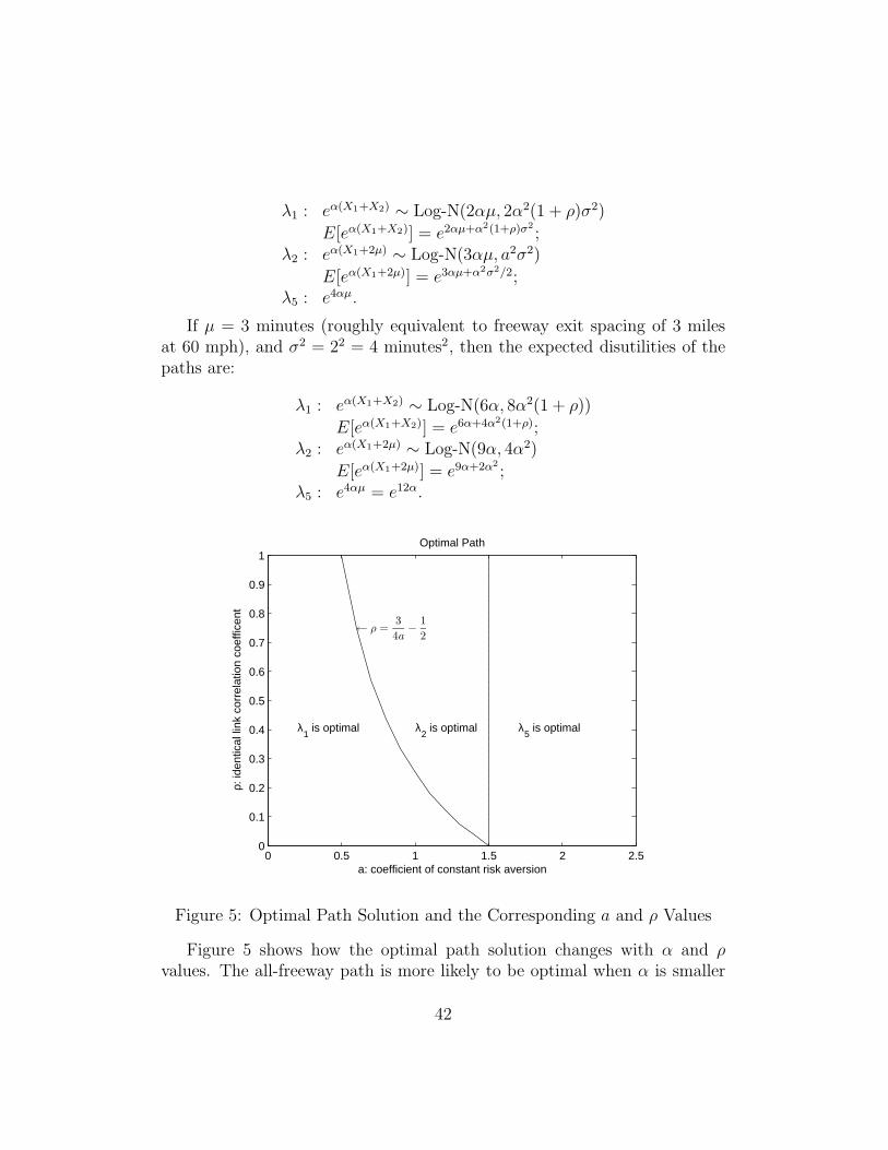
λ1 : eα(X1+X2) ∼ Log-N(2αµ, 2α2(1 + ρ)σ2)

E[eα(X1+X2)] = e2αµ+α2(1+ρ)σ2

;λ2 : eα(X1+2µ) ∼ Log-N(3αµ, a2σ2)

E[eα(X1+2µ)] = e3αµ+α2σ2/2;λ5 : e4αµ.

If µ = 3 minutes (roughly equivalent to freeway exit spacing of 3 milesat 60 mph), and σ2 = 22 = 4 minutes2, then the expected disutilities of thepaths are:

λ1 : eα(X1+X2) ∼ Log-N(6α, 8α2(1 + ρ))

E[eα(X1+X2)] = e6α+4α2(1+ρ);λ2 : eα(X1+2µ) ∼ Log-N(9α, 4α2)

E[eα(X1+2µ)] = e9α+2α2

;λ5 : e4αµ = e12α.

0 0.5 1 1.5 2 2.50

0.1

0.2

0.3

0.4

0.5

0.6

0.7

0.8

0.9

1

a: coefficient of constant risk aversion

ρ: id

entic

al li

nk c

orre

latio

n co

effic

ent

Optimal Path

λ1 is optimal λ

2 is optimal λ

5 is optimal

← ρ =3

4a−

1

2

Figure 5: Optimal Path Solution and the Corresponding a and ρ Values

Figure 5 shows how the optimal path solution changes with α and ρvalues. The all-freeway path is more likely to be optimal when α is smaller

42

(suggesting an attitude closer to risk neutrality) and ρ is smaller, similar tothe results from the computational tests in Section 5.2.

Specifically, when α < 0.5, the all-freeway path λ1 is optimal regardlessof the correlation. When 0.5 < α < 1.5, the all-freeway path λ1 is optimalfor low correlations, and the freeway-local path λ2 is optimal for high corre-lations. The boundary dividing “low” and “high” correlations changes withα as specified by the equation in Figure 5. Note that the boundary is derivednumerically in the computational tests. When α > 1.5, the all-local path λ5

is optimal regardless of the correlation.For normally distributed variables, independence is equivalent to zero

correlation coefficient. If the stochastic dependencies are ignored as in mostexisting studies, the horizontal line in Figure 5 with ρ = 0 shows that thefreeway-local path can never be an optimal path regardless of the risk aversionlevel, and the all-freeway path is always optimal for α < 1.5, which can beviewed as a reasonable range for an average person’s risk aversion parameter.This is due to the underestimation of the all-freeway path risk by assumingstochastic independence between links.

C. Glossary

Support point:A distinct value (vector of values) that a discrete random variable (vec-

tor) can take. C = C1, . . . , CR is the set of support points of the jointprobability mass function of all link travel times at all time periods, whereCr is a vector of time-dependent link travel times with a dimension of K×m(K is the number of time periods andm the number of links), r = 1, 2, . . . , R.Cr

jk,t is the travel time of link (j, k) at time t in the r-th support point, with

probability pr, andR∑

r=1

pr = 1.

Support point disutility Dλ(O, t, r):The disutility of path λ from origin node O and departure time t to the

destination node D in support point r. If the disutility is travel time itself,then Dλ(O, t, r) = Sλ(O, t, r), which is support point travel time.

Expected disutility dλ(O, t):The expected disutility of path λ from origin node O and departure

43

time t to the destination node D. If the disutility is travel time itself, thendλ(O, t) = eλ(O, t), which is expected travel time.

Path with MED for departure time t:A path λ with MED from origin O to destination D for departure time

t has the minimum expected disutility over all support points among all thepaths between the same OD pair and for the same departure time, i.e., ∃ nopath λ′ such that dλ′(O, t) < dλ(O, t).

The complete time-support-point set Ω:The Cartesian product of the sets of time periods T and support points

C, that is, Ω = (t, r)|t ∈ T, r ∈ C.

Non-Dominated Path:A path λ from origin O to destination D is non-dominated w.r.t. a subset

Ω′ of Ω iff ∃ no other path λ′ between the same OD pair such thatDλ′(O, t, r) ≤ Dλ(O, t, r), ∀(t, r) ∈ Ω′ and∃(t0, r0) ∈ Ω′ such that Dλ′(O, t0, r0) < Dλ(O, t0, r0).If not specified, non-dominance is w.r.t. the complete set of departure

time and support points Ω.

Pure Path:A path is pure iff the path itself and all its sub-paths are non-dominated

w.r.t. the complete set of departure time and support points Ω; otherwise,it is a mixed path.

Risk aversion factor a:The parameter in the disutility function of travel time which represents

the traveler’s risk aversion. In the exponential disutility function exp(aX),the value of α shows the level of the traveler’s risk aversion. A larger α isassociated with a higher level of risk aversion.

Identical correlation coefficient ρ:In the computational tests, we assume identical correlation coefficient

between any pair of link travel time random variables. In other words, inthe correlation matrix of link travel time random variables, all non-diagonalelements are the same.

44