optimal paths in gliding flight - virginia tech
TRANSCRIPT

Optimal Paths in Gliding Flight
Artur Wolek
Dissertation submitted to the Faculty of the
Virginia Polytechnic Institute and State University
in partial fulfillment of the requirements for the degree of
Doctor of Philosophy
in
Aerospace Engineering
Craig A. Woolsey, Chair
Eugene M. Cliff
Leigh S. McCue-Weil
Daniel J. Stilwell
May 1, 2015
Blacksburg, Virginia
Keywords: path planning, nonlinear optimal control, underwater gliders

Optimal Paths in Gliding Flight
Artur Wolek
Abstract
Underwater gliders are robust and long endurance ocean sampling platforms that are increas-
ingly being deployed in coastal regions. This new environment is characterized by shallow
waters and significant currents that can challenge the mobility of these efficient (but tradi-
tionally slow moving) vehicles. This dissertation aims to improve the performance of shallow
water underwater gliders through path planning.
The path planning problem is formulated for a dynamic particle (or “kinematic car”)
model. The objective is to identify the path which satisfies specified boundary conditions
and minimizes a particular cost. Several cost functions are considered. The problem is
addressed using optimal control theory. The length scales of interest for path planning are
within a few turn radii.
First, an approach is developed for planning minimum-time paths, for a fixed speed glider,
that are sub-optimal but are guaranteed to be feasible in the presence of unknown time-
varying currents. Next the minimum-time problem for a glider with speed controls, that
may vary between the stall speed and the maximum speed, is solved. Last, optimal paths
that minimize change in depth (equivalently, maximize range) are investigated.
Recognizing that path planning alone cannot overcome all of the challenges associated
with significant currents and shallow waters, the design of a novel underwater glider with
improved capabilities is explored. A glider with a pneumatic buoyancy engine (allowing
large, rapid buoyancy changes) and a cylindrical moving mass mechanism (generating large
pitch and roll moments) is designed, manufactured, and tested to demonstrate potential
improvements in speed and maneuverability.

In loving memory of my grandparents
iii

Acknowledgments
I thank my advisor, Craig Woolsey, for his steadfast support and guidance throughout my
academic career. Starting from my days as an undergraduate student in his lab, through my
graduate studies, he has been an inspiring mentor and a source of boundless patience and
optimism. I am honored to be his student.
I thank the faculty and staff of the Aerospace and Ocean Engineering department at
Virginia Polytechnic Institute and State University for providing a great environment in
which to study. I am grateful for the support of my committee members Leigh McCue-
Weil and Daniel Stilwell. I would especially like to acknowledge Eugene Cliff who strongly
influenced the direction of my research, and who humbled me with his knowledge of optimal
control. I was lucky to meet many colleagues and friends along the way who also became
invaluable resources. In particular, I thank Ony Arifianto, Matt Giarra, Dave Grymin,
Andrew Rogers, and Sevak Tahmasian for their discussions regarding my work. I am also
grateful for all of the current and past members of the Nonlinear Systems Laboratory who
made the lab an enjoyable place.
I have had the unique opportunity to conduct applied research and design and test an
underwater glider. This was a rewarding experience that gave me an appreciation for the
challenges associated with taking a design from the drawing board and making it really work.
I would like to thank Tom Swean and the Office of Naval Research for their sponsorship under
grant N00014-13-1-0060. The glider project would not have been possible without the help of
our collaborators at the University of Washington, namely Kristi Morgansen, Jake Quenzer
and Laszlo Techy. I would also like to thank James Burns and Jonathan Murrow for their
dedication to this project. I especially would like to acknowledge the effort of Tejaswi Gode
who developed the acoustic positioning and communication system and helped with field
trials. I also appreciate the many undergraduate volunteers involved over the years.
I will be forever grateful for my parents’ love and encouragement. I appreciate the sacri-
fices they made so that I could have this opportunity. I also thank all of my loved ones and
friends for their support.
iv

Contents
List of Figures ix
List of Tables xiii
1 Introduction 1
1.1 Motivation . . . . . . . . . . . . . . . . . . . . . . . . . . . . . . . . . . . . . 3
1.2 Review: Glider Motion Control Approaches . . . . . . . . . . . . . . . . . . 3
1.2.1 Vehicle-Scale Motion Control . . . . . . . . . . . . . . . . . . . . . . 4
1.2.2 Micro-Scale Path Planning . . . . . . . . . . . . . . . . . . . . . . . . 5
1.2.3 Synoptic-Scale Path Planning . . . . . . . . . . . . . . . . . . . . . . 8
1.3 Outline and Contributions . . . . . . . . . . . . . . . . . . . . . . . . . . . . 10
2 Mathematical Preliminaries 14
2.1 An Optimal Control Problem . . . . . . . . . . . . . . . . . . . . . . . . . . 14
2.2 Pontryagin’s Minimum Principle . . . . . . . . . . . . . . . . . . . . . . . . . 16
2.3 Indirect and Direct Methods . . . . . . . . . . . . . . . . . . . . . . . . . . . 18
2.4 The Hodograph . . . . . . . . . . . . . . . . . . . . . . . . . . . . . . . . . . 22
2.5 Karush-Kuhn-Tucker (KKT) Conditions . . . . . . . . . . . . . . . . . . . . 24
2.6 An Existence Theorem for Optimal Controls . . . . . . . . . . . . . . . . . . 26
2.7 Dubins Path Planning . . . . . . . . . . . . . . . . . . . . . . . . . . . . . . 27
3 Feasible Paths in Unknown, Unsteady Currents 30
3.1 Introduction . . . . . . . . . . . . . . . . . . . . . . . . . . . . . . . . . . . . 30
v
3.2 Problem Formulation . . . . . . . . . . . . . . . . . . . . . . . . . . . . . . . 31
3.3 Tradeoff Between Path Length and Path Feasibility . . . . . . . . . . . . . . 34
3.4 Path Following Performance . . . . . . . . . . . . . . . . . . . . . . . . . . . 36
3.5 Conclusion . . . . . . . . . . . . . . . . . . . . . . . . . . . . . . . . . . . . . 40
4 Time-Optimal Path Planning with Variable Speed Controls 41
4.1 Introduction . . . . . . . . . . . . . . . . . . . . . . . . . . . . . . . . . . . . 41
4.2 Problem Formulation . . . . . . . . . . . . . . . . . . . . . . . . . . . . . . . 43
4.3 Applying the Minimum Principle . . . . . . . . . . . . . . . . . . . . . . . . 45
4.4 Geometric Approach - the Hodograph . . . . . . . . . . . . . . . . . . . . . . 46
4.5 Existence of An Optimal Control . . . . . . . . . . . . . . . . . . . . . . . . 51
4.6 Properties of Extremal Controls . . . . . . . . . . . . . . . . . . . . . . . . . 51
4.7 Additional Optimality Conditions . . . . . . . . . . . . . . . . . . . . . . . . 60
4.8 Path Synthesis . . . . . . . . . . . . . . . . . . . . . . . . . . . . . . . . . . 63
4.9 Illustrative Examples . . . . . . . . . . . . . . . . . . . . . . . . . . . . . . . 66
4.10 Conclusion . . . . . . . . . . . . . . . . . . . . . . . . . . . . . . . . . . . . . 68
5 Energy-Optimal Path Planning with a Quadratic Glide Polar 71
5.1 Introduction . . . . . . . . . . . . . . . . . . . . . . . . . . . . . . . . . . . . 71
5.2 The Glide Polar . . . . . . . . . . . . . . . . . . . . . . . . . . . . . . . . . . 73
5.3 Problem Formulation . . . . . . . . . . . . . . . . . . . . . . . . . . . . . . . 76
5.4 Existence of an Optimal Control . . . . . . . . . . . . . . . . . . . . . . . . . 77
5.5 Applying the Minimum Principle . . . . . . . . . . . . . . . . . . . . . . . . 78
5.6 Properties of Extremal Controls . . . . . . . . . . . . . . . . . . . . . . . . . 79
5.7 Additional Optimality Conditions . . . . . . . . . . . . . . . . . . . . . . . . 84
5.8 Path Synthesis . . . . . . . . . . . . . . . . . . . . . . . . . . . . . . . . . . 92
5.9 Illustrative Examples . . . . . . . . . . . . . . . . . . . . . . . . . . . . . . . 94
5.10 Conclusion . . . . . . . . . . . . . . . . . . . . . . . . . . . . . . . . . . . . . 99
6 Energy-Optimal Path Planning with Speed and Load Factor Controls 101
vi

6.1 Introduction . . . . . . . . . . . . . . . . . . . . . . . . . . . . . . . . . . . . 101
6.2 Gliding and Turning Flight . . . . . . . . . . . . . . . . . . . . . . . . . . . . 102
6.3 Problem Formulation . . . . . . . . . . . . . . . . . . . . . . . . . . . . . . . 104
6.4 Applying the Minimum Principle . . . . . . . . . . . . . . . . . . . . . . . . 108
6.5 Geometrical Approach - the Hodograph . . . . . . . . . . . . . . . . . . . . . 109
6.6 Existence of An Optimal Control . . . . . . . . . . . . . . . . . . . . . . . . 112
6.7 Analytical Approach . . . . . . . . . . . . . . . . . . . . . . . . . . . . . . . 113
6.8 Path Synthesis . . . . . . . . . . . . . . . . . . . . . . . . . . . . . . . . . . 123
6.9 Conclusion . . . . . . . . . . . . . . . . . . . . . . . . . . . . . . . . . . . . . 126
7 Design and Testing of a Pneumatically Propelled Underwater Glider 128
7.1 Introduction . . . . . . . . . . . . . . . . . . . . . . . . . . . . . . . . . . . . 128
7.2 Buoyancy Control . . . . . . . . . . . . . . . . . . . . . . . . . . . . . . . . . 131
7.3 Attitude Control . . . . . . . . . . . . . . . . . . . . . . . . . . . . . . . . . 145
7.4 Wing and Tail Design . . . . . . . . . . . . . . . . . . . . . . . . . . . . . . 148
7.5 Electronics and Software . . . . . . . . . . . . . . . . . . . . . . . . . . . . . 152
7.6 Acoustic Positioning and Communication . . . . . . . . . . . . . . . . . . . . 153
7.7 Testing . . . . . . . . . . . . . . . . . . . . . . . . . . . . . . . . . . . . . . . 155
7.8 Conclusion . . . . . . . . . . . . . . . . . . . . . . . . . . . . . . . . . . . . . 163
8 Conclusions 167
Appendix A Deriving the Feasible Turn Radius R′0 170
Appendix B Sub-Optimality Conditions for Minimum-Time Paths 175
B.1 Analytical Approach to the min-H Operation . . . . . . . . . . . . . . . . . 175
B.2 Sub-Optimality Conditions for Symmetric Turns TFS and TRS . . . . . . . . . 179
B.3 Sub-Optimality Conditions for ST FB and TFBS Extremals . . . . . . . . . . 180
B.4 Sub-Optimality Conditions for BT RSB Extremals . . . . . . . . . . . . . . . 188
Appendix C Minimum-Energy Extremals for a Quadratic Glider Polar 191
vii
C.1 Parameterizing Extremal Controls . . . . . . . . . . . . . . . . . . . . . . . . 191
C.2 Solving for BSB Extremals . . . . . . . . . . . . . . . . . . . . . . . . . . . . 193
C.3 Solving for BBBB Extremals . . . . . . . . . . . . . . . . . . . . . . . . . . . 196
C.4 Solving for BstallBstallBstallBstall and Bms Extremals . . . . . . . . . . . . . . . 197
9 Bibliography 199
viii
List of Figures
1.1 Length scales of glider motion . . . . . . . . . . . . . . . . . . . . . . . . . . 4
2.1 A generic hodograph. Adapted from (Cliff et al., 1993). . . . . . . . . . . . . 24
2.2 Candidate Dubins paths for a given endpoint x1 . . . . . . . . . . . . . . . . 29
3.1 Partitions of the configuration space for final course angles ψ1 = 0, 2π/3 andπ, respectively . . . . . . . . . . . . . . . . . . . . . . . . . . . . . . . . . . . 33
3.2 Contour maps of the ratio of optimal path lengths planned using R′0 and R0 34
3.3 Comparison of closed-loop path following performance (solid lines) for pathsplanned to the state x1 using turn radii R0 (dashed line) and R′0 (dashed-dotted line) . . . . . . . . . . . . . . . . . . . . . . . . . . . . . . . . . . . . 37
3.4 Normalized mean, final cross-track error versus Rplan from Monte Carlo sim-ulation . . . . . . . . . . . . . . . . . . . . . . . . . . . . . . . . . . . . . . . 39
4.1 Control constraint set Ω . . . . . . . . . . . . . . . . . . . . . . . . . . . . . 45
4.2 The hodograph set, with subspaces of constant Hc drawn (dotted lines), for agiven adjoint vector . . . . . . . . . . . . . . . . . . . . . . . . . . . . . . . . 48
4.3 Types of extremal paths . . . . . . . . . . . . . . . . . . . . . . . . . . . . . 50
4.4 Generic solution where ηψ does not change sign or does not vanish over aninterval . . . . . . . . . . . . . . . . . . . . . . . . . . . . . . . . . . . . . . . 53
4.5 Generic solution where ηψ intersects the s-axis tangentially . . . . . . . . . . 56
4.6 Generic solution where ηψ intersects the s-axis transversally . . . . . . . . . 57
4.7 Locally optimal paths from the set ΓT T T T ∪ ΓT ST ∪ Γumax for the terminalstate x1 = (0 2 2π/3)T . . . . . . . . . . . . . . . . . . . . . . . . . . . . 67
4.8 Locally optimal paths from ΓDubins for the terminal state x1 = (0 2 2π/3)T 68
ix

4.9 Lowest-cost paths for a grid of terminal states with ψ1 = 0 . . . . . . . . . . 69
4.10 Lowest-cost paths for a grid of terminal states with ψ1 = 2π/3 . . . . . . . . 69
4.11 Lowest-cost paths for a grid of terminal states with ψ1 = π . . . . . . . . . . 70
5.1 A typical glide polar . . . . . . . . . . . . . . . . . . . . . . . . . . . . . . . 74
5.2 A sub-optimal BstallBstallBstallBstall extremal sequence . . . . . . . . . . . . . 86
5.3 The sequence of three B extremal arcs, that each begin and end with ηψ = 0,is sub-optimal . . . . . . . . . . . . . . . . . . . . . . . . . . . . . . . . . . . 91
5.4 Digitized glide polar of the DG-1001M motorglider (dashed line), adaptedfrom DG Flugzeugbau Gmbh (2010), compared to a quadratic approximation(solid line) . . . . . . . . . . . . . . . . . . . . . . . . . . . . . . . . . . . . . 95
5.5 Path synthesis result for the normalized final state x1 = (0 1 2π/3)T . . . 97
5.6 Path synthesis result for the normalized final state x1 = (−3 4 0)T . . . . 98
5.7 Path synthesis result for the normalized final state x1 = (0 2 7π/4)T . . . 99
6.1 Longitudinal forces in a steady gliding turn . . . . . . . . . . . . . . . . . . . 102
6.2 Lateral forces in a steady gliding turn . . . . . . . . . . . . . . . . . . . . . . 102
6.3 The control constraint set Ω . . . . . . . . . . . . . . . . . . . . . . . . . . . 107
6.4 The hodograph set is the image of Ω under the mapping (6.29). (Refer toFigure 6.3 for description of the line types.) . . . . . . . . . . . . . . . . . . 111
6.5 Extremal controls and corresponding separating planes, along the hodographboundary, with increasing |ηψ| . . . . . . . . . . . . . . . . . . . . . . . . . . 112
6.6 Sketch of the control contrain set and hodograph of the relaxed problem . . 113
6.7 The turn polar . . . . . . . . . . . . . . . . . . . . . . . . . . . . . . . . . . 114
6.8 The dog house plot . . . . . . . . . . . . . . . . . . . . . . . . . . . . . . . . 114
6.9 Speed history along the extremal locus, for various parameters p3 . . . . . . 119
6.10 Load factor history along the stall boundary, for various parameters p3 . . . 122
6.11 Locally optimal solution for x1 = (−2 4 7π/4)T . . . . . . . . . . . . . . . 125
6.12 Locally optimal solution for x1 = (0 − 0.5 π)T . . . . . . . . . . . . . . . 126
6.13 Locally optimal solution for x1 = (1.1 2 0)T . . . . . . . . . . . . . . . . . 127
7.1 Major components of the Virginia Tech Underwater Glider . . . . . . . . . . 129
x

7.2 The Virginia Tech Underwater Glider . . . . . . . . . . . . . . . . . . . . . . 130
7.3 Number of dives . . . . . . . . . . . . . . . . . . . . . . . . . . . . . . . . . . 136
7.4 Net weight with bladder volume for various scuba tank weights . . . . . . . . 137
7.5 Experiment for determining bladder pressure vs. buoyancy curve . . . . . . . 138
7.6 Bladder open loop response . . . . . . . . . . . . . . . . . . . . . . . . . . . 139
7.7 Inflator and deflator requirements . . . . . . . . . . . . . . . . . . . . . . . . 141
7.8 Sizing the pneumatic buoyancy engine control valves for a fixed bladder volume143
7.9 Pneumatic buoyancy engine schematic . . . . . . . . . . . . . . . . . . . . . 144
7.10 Interior and exterior of the buoyancy control system . . . . . . . . . . . . . . 145
7.11 Unstable (open-loop) bladder pressure and depth rate coupling . . . . . . . . 146
7.12 Forces acting on the glider in an steady equilibrium pitch attitude . . . . . . 147
7.13 Longitudinally moving actuator . . . . . . . . . . . . . . . . . . . . . . . . . 148
7.14 Rotating moving mass actuator . . . . . . . . . . . . . . . . . . . . . . . . . 148
7.15 Range of asymmetric geometries provided by the wing harness . . . . . . . . 149
7.16 Longitudinal forces in a steady gliding turn . . . . . . . . . . . . . . . . . . . 150
7.17 Spider plot: predicted performance of a hypothetical Seaglider equipped witha high displacement bladder. Lines of constant flight path angle (green) andangle of attack (red) are superimposed. . . . . . . . . . . . . . . . . . . . . . 151
7.18 Drop-weight design . . . . . . . . . . . . . . . . . . . . . . . . . . . . . . . . 152
7.19 Types of acoustic baseline geometries. Used with permission (Gode, 2015). . 154
7.20 Beacon deployed on a raft. Used with permission (Gode, 2015). . . . . . . . 155
7.21 Feasibility test of the pneumatic buoyancy engine . . . . . . . . . . . . . . . 156
7.22 Lake Washington Depth Rating Test . . . . . . . . . . . . . . . . . . . . . . 157
7.23 Pool sawtooth test . . . . . . . . . . . . . . . . . . . . . . . . . . . . . . . . 158
7.24 Buoyancy engine tests at Claytor Lake, VA . . . . . . . . . . . . . . . . . . . 159
7.25 Glider in a communications stance . . . . . . . . . . . . . . . . . . . . . . . 160
7.26 Path of the boat (with onboard glider) during the test at Claytor Lake, VA(Map data from Google Earth). Used with permission (Gode, 2015). . . . . . 161
7.27 Testing the LBL system with a GPS-equipped boat emulating the glider usingNorth-South oriented swaths (Track 1). Used with permission (Gode, 2015). 162
xi
7.28 Sawtooth glide test with acoustic positioning . . . . . . . . . . . . . . . . . . 164
7.29 Sawtooth glide test with acoustic positioning and attitude control . . . . . . 165
8.1 Varying environmental conditions and objectives may require a number ofdifferent planning approaches to be employed. . . . . . . . . . . . . . . . . . 168
B.1 Symmetric turn with α = αsubopt . . . . . . . . . . . . . . . . . . . . . . . . 179
B.2 Contours of g(α, β) with the feasible set indicated as the triangular region, forψ ≤ π, and as the trapezoidal region for ψ > π . . . . . . . . . . . . . . . . . 182
B.3 Admissible ∆y for ψ ≤ π . . . . . . . . . . . . . . . . . . . . . . . . . . . . . 182
B.4 Admissible ∆y for ψ > π . . . . . . . . . . . . . . . . . . . . . . . . . . . . . 183
B.5 Suboptimal case: β > π . . . . . . . . . . . . . . . . . . . . . . . . . . . . . 186
B.6 Suboptimal case: γ > γmin . . . . . . . . . . . . . . . . . . . . . . . . . . . . 187
B.7 BTRSB segment with equal initial and final B arcs . . . . . . . . . . . . . . . 188
B.8 Case A: Joining two circles a distance 0 < d < 2(R + r) apart . . . . . . . . 190
xii
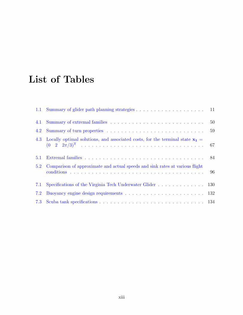
List of Tables
1.1 Summary of glider path planning strategies . . . . . . . . . . . . . . . . . . . 11
4.1 Summary of extremal families . . . . . . . . . . . . . . . . . . . . . . . . . . 50
4.2 Summary of turn properties . . . . . . . . . . . . . . . . . . . . . . . . . . . 59
4.3 Locally optimal solutions, and associated costs, for the terminal state x1 =(0 2 2π/3)T . . . . . . . . . . . . . . . . . . . . . . . . . . . . . . . . . . 67
5.1 Extremal families . . . . . . . . . . . . . . . . . . . . . . . . . . . . . . . . . 84
5.2 Comparison of approximate and actual speeds and sink rates at various flightconditions . . . . . . . . . . . . . . . . . . . . . . . . . . . . . . . . . . . . . 96
7.1 Specifications of the Virginia Tech Underwater Glider . . . . . . . . . . . . . 130
7.2 Buoyancy engine design requirements . . . . . . . . . . . . . . . . . . . . . . 132
7.3 Scuba tank specifications . . . . . . . . . . . . . . . . . . . . . . . . . . . . . 134
xiii

Chapter 1
Introduction
Ocean sensing for science, commerce, and defense applications is increasingly being carried
out by autonomous underwater vehicles (AUVs). Improvements in vehicle autonomy, plat-
form technologies, energy storage and cost have motivated the use of these marine robots to
replace manned vessels, instrumented buoys and remotely operated vehicles in ocean sam-
pling applications. As reliance on AUVs increases further, the need arises to deploy them for
longer periods of time, and with less human intervention. AUVs are operating in increasingly
complex and dynamic environments, such as the coastal ocean. Motion planning and control
is a basic area of research that will enable and facilitate their widespread use.
In the coastal ocean, sunlight penetrates the shallow waters creating a euphotic zone
that hosts many plants, algae, reefs and other organisms of interest to marine biologists or
of commercial value to industry. Physical oceanographers study this region for its diverse
interaction of many physical processes such as coastal currents, internal waves, river discharge
and estuarine features. The littoral zone is also the setting for reconnaissance, surveillance,
mine counter-measure and anti-submarine warfare operations that are of strategic importance
to the Navy. However, this environment also presents several challenges for AUVs. The
1
Chapter 1. Introduction
presence of significant currents that are often dynamic and complex can adversely affect the
mobility and efficiency of AUVs. Moreover, the increased rate of biofouling in the euphotic
zone can cripple long endurance robotic platforms.
Underwater gliders are a class of AUVs that have been used extensively in long endurance,
deep sea, ocean sampling applications (Bachmayer et al., 2004). Gliders are flight vehicles
that use potential energy for propulsion. By actively adjusting their buoyancy, gliders can
move up and down through the water column. Lift generated by the glider’s wings con-
verts this vertical motion into forward flight. (Unlike a conventional flight vehicle, a glider
has no thruster or propeller.) Gliders are capable of traversing thousands of kilometers
over deployment times of weeks, or months, because their motion largely consists of steady,
stable, low power glides. Energy intensive buoyancy changes occur infrequently. The lack
of external moving parts makes gliders quiet (and stealthy). This also makes them more
robust to corrosion or biofouling than their propeller driven counterparts with external mov-
ing control surfaces. From robustness and endurance considerations, underwater gliders are
ideal candidates for shallow water operations. However, they suffer from their slow speeds
(between 20-30 cm/s) and poor maneuverability which can compromise their locomotive effi-
ciency. Often times the ambient current magnitude can be a significant fraction of the glider’s
speed, and can potentially dominate its dynamics. This problem is exacerbated by the fact
that position measurements are typically unavailable while the vehicle is underway. (Global
positioning system (GPS) fixes are obtained only on the surface, and acoustic positioning
requires infrastructure that is not always available.) This lack of position information makes
underwater navigation particularly difficult. Underwater gliders can serve as reliable, long
endurance, coastal ocean sampling platforms if their ability to operate in shallow waters and
significant currents can be improved.
2

Chapter 1. Introduction
1.1 Motivation
The performance of a glider is determined in part by its inherent design (i.e. actuator
capabilities, hydrodynamics, and energy storage) and in part by the way it is operated (i.e.
guidance, navigation, and control). The goal of this work is to improve the capabilities of
underwater gliders operating in shallow waters and significant currents. Specifically, our
objective is to:
1. develop path planning approaches that improve robustness in currents, minimize transit
time, or maximize range,
2. and to demonstrate the use of novel actuators that can improve the glider’s maneuver-
ability, speed, and hydrodynamic efficiency.
Improvements in maneuverability and motion control may enable new operational paradigms
for gliders, for example: to operate in constrained and cluttered environments such as ports or
harbors, to enable precision positioning of directional sensors, or docking with other vehicles.
Some aspects of this work may also be relevant to other gliding vehicles such as: sailplanes,
conventional powered aircraft in emergencies (planning glides to the nearest runway after
engine failure (Atkins et al., 2006)), unmanned aerial vehicles (to increase endurance by
gliding (Edwards and Silberberg, 2010)) or even buoyancy-driven gliders proposed to explore
the moons of other planets (Morrow et al., 2006; Allen et al., 2013).
1.2 Review: Glider Motion Control Approaches
The guidance, navigation, and control system of an underwater glider takes inputs from a
high level mission planner, or directly from a human operator, and coordinates the glider’s
3

Chapter 1. Introduction
motion to achieve some objective. One approach to glider motion control is a hierarchical ap-
proach that decomposes the objective into several characteristic length scales (see Figure 1.1)
and time constants of motion, as discussed by Techy (2011).
On the smallest vehicle-scale the objective is to develop a control law to achieve and
regulate a stable and steady motion. The micro-scale refers to lengths on the order of
several turn radii of the vehicle where steady motions can be concatenated to maneuver the
vehicle into a desired position, and heading, while accounting for local flow features. Last,
the synoptic-scale is the largest length scale where the glider traverses large distances through
a flow field that is often spatially and temporally varying. At each of these length scales,
1 meter
100+ m
10+ km
Vehicle-Scale
Micro-Scale
Synoptic-Scale
Figure 1.1: Length scales of glider motion
different vehicle and flow field models are appropriate to capture the relevant dynamics. This
dissertation presents several micro-scale path planning methods. To place these contributions
in context some fundamental control approaches of all three scales of motion are briefly
discussed.
1.2.1 Vehicle-Scale Motion Control
On the length scale of the vehicle, the control objective is typically to obtain a stable feedback
controller that can achieve a desired steady-state motion. Having done so, one may inves-
tigate robustness to unmodeled dynamics and disturbances or adapt the control strategy to
enable trajectory tracking. A nonlinear rigid body dynamic model of the glider, subject to
4

Chapter 1. Introduction
forces and moments, can be used for control design and analysis, see (Graver, 2005; Bhatta,
2006; Mahmoudian, 2009). In cases where flow gradients are strong, a more general model
may be used (Thomasson and Woolsey, 2013).
Traditionally, a bang-bang or PID (proportional-integral-derivative) feedback control loop
is used to control the vehicle state associated with each actuator: depth rate with the buoy-
ancy engine, pitch with the longitudinal moving mass, and roll with the lateral moving mass,
as discussed by Bachmayer et al. (2003) and Jenkins et al. (2003). Actuator nonlinearities
such as deadzones and saturations are introduced to reduce actuator effort and improve en-
ergy efficiency. These inner control loops can be nested inside an outer control loop that
regulates higher level behavior (such as turn rate and flight path angle). Further, these outer
control loops can be augmented using “feed-forward” commands that give approximate ac-
tuator positions for steady motions (Mahmoudian, 2009). Such feed-forward commands can
be based on analytical models, or experimentally derived look-up tables. Other approaches
for regulating steady motions use linear optimal control (Leonard and Graver, 2001) or Lya-
punov based methods (Bhatta and Leonard, 2008). Fuzzy logic (Kanakakis et al., 2004)
and passivity based controllers (Zhang et al., 2012) have also been proposed. Trajectory
optimization can be used to optimize transient motions on the vehicle-scale. For exam-
ple, in (Kraus, 2010) optimal schedules for buoyancy and pitch changes were determined to
efficiently transition from a dive to a climb, avoiding stall.
1.2.2 Micro-Scale Path Planning
The micro-scale refers to a length scale between tens and hundreds of meters. Such distances
are on the order of a few turn radii of a typical glider. Thus, one must consider the vehicle’s
turning dynamics. Often the objective is to achieve a desired planar position and heading.
5
Chapter 1. Introduction
(In most applications, gliders are used to profile the water column by continuously changing
their depth. It is uncommon for a glider’s mission objective to require attaining a planar
position and depth simultaneously, however one can imagine or contrive a scenario where
this may be required.) On this scale, it may be sufficient to assume a rather simple local
flow field (for example, uniform and steady currents). The relevant motions are those in
which the position and orientation of the glider is important (e.g. to change course angle,
point a directional sensor, or avoid an obstacle). Micro-scale maneuvers can also be used as
primitive motions for larger, more complex, synoptic-scale planning algorithms.
In (Mahmoudian et al., 2010) an approximate analytical expression for the steady turning
motion of a glider was derived using perturbation theory and a realistic multi-rigid-body
dynamic model of a glider. It was shown that if one views the glider’s motion from above,
then a glider operating at a fixed glide slope appears as a constant speed planar vehicle
with a bounded turn rate. This model of vehicle motion, in which the glider always moves
in the direction it is pointed, with turn-rate controls, is often called a “kinematic car” or a
“Dubins car”. The latter term refers to L.E. Dubins, who characterized the paths of minimum
length for this vehicle model (Dubins, 1957). These minimum-length “Dubins paths” can be
constructed using a simple, geometric procedure. For this reason they are widely used for
guidance of constant-speed, planar vehicles (Djath et al., 1999; Chitsaz and LaValle, 2007).
Dubins’ problem has been extended by numerous authors to account for additional vehi-
cle dynamics and environmental disturbances or dependencies. Often, the structure of the
optimal control is first elucidated by deriving a finite and sufficient set of candidate optimal
controls, as Dubins did. The synthesis problem of constructing a minimum time path that
meets the two boundary conditions can then be solved. Reeds and Shepp (1990) derived a
sufficient set of candidate controls for a car that moves both forward and backward at fixed
speeds. Later Boissonnat et al. (1992) used Pontryagin’s Minimum Principle and Sussmann
6

Chapter 1. Introduction
and Tang (1991) used geometric optimal control techniques to address the same problem.
The path synthesis problem was solved by Bui et al. (1994) for the Dubins case and by
Soueres and Laumond (1996) for the Reeds and Shepp case. In general, these paths consist
of straight line segments and circular arcs, sometimes yielding cusps when the car is al-
lowed to move in reverse. Therefore these paths contain discontinuities in the curvature. To
produce paths with continuous curvature, the optimal control problem can be reformulated
to include turn acceleration bounds in the vehicle’s motion model. Through the work of
Boissonnat et al. (1994), Sussmann (1997) and Degtiariova-Kostova and Kostov (1998), it
was shown that the optimal path in this case consists of straight segments, circular arcs and
clothoids. Further, the optimal path may contain infinitely many clothoids (a “chattering”
solution), which complicates the path synthesis problem. A practical approach, taken in
(Scheuer and Fraichard, 1997; Fraichard and Scheuer, 2004), was to construct a sub-optimal
path that incorporates a finite number of clothoidal segments ensuring the path has both a
bounded curvature and a bounded rate of curvature.
For flight vehicle applications, extensions of the Dubins problem have incorporated various
flow fields (winds or currents). Path planning in a steady, uniform flow field was considered
by McGee and Hedrick (2007), Techy and Woolsey (2009) and Bakolas and Tsiotras (2010).
Turn acceleration limits were considered by Techy et al. (2010b). The case of a known,
unsteady flow field was studied by McNeely et al. (2007).
Maggiar and Dolinskaya (2014) considered path planning for a vehicle model where the
speed and the maximum turn rate are heading dependent. (This approach can be used to
model the effects of a flow field.) Sanfelice and Frazzoli (2008) considered a heterogeneous
terrain where the vehicle’s speed varies discontinuously in two distinct regions of the plane.
Herisse and Pepy (2013) considered the case where the turn rate is position dependent. Pepy
and Herisse (2014) also studied a related problem, in the vertical plane, where the goal is to
7

Chapter 1. Introduction
maximizing the terminal velocity of a glider with pitch rate controls.
Several authors have also extended the Dubins problem to account for vehicle-specific
dynamics. Shapira and Ben-Asher (1997) approximated the thrust limit of an aircraft by
taking the speed to be a function of the turn rate. The minimum time path problem for a
vehicle with asymmetric turn limits (i.e. with a damaged steering mechanism, or a preferred
turning direction) was studied by Bakolas and Tsiotras (2011). Choi and Atkins (2010)
investigated a related problem for a vehicle with a hardware failure, but restricted the turns
to be within a minimum and maximum turning radius, and did not allow straight segments
(so that the vehicle is always turning).
1.2.3 Synoptic-Scale Path Planning
For path planning on the length scale of large ocean weather systems (the synoptic scale
on the order of kilometers) spatially and temporally varying flow fields and obstacles must
be considered. On these length scales, the turning segments of a glider becomes negligible
and a simple particle model, with the heading as a control input, often suffices to accurately
describe the glider’s motion.
The most basic navigational approach, when no flow field information is available, is to
follow a straight line path to the desired waypoint with constant heading and glide angle
(Webb et al., 2001). By comparing sequences of dead reckoned position estimates to mea-
surements from GPS fixes obtained after surfacing, a Kalman filter can be used to estimate
currents. This information can then be used to choose a corrected heading and glide angle
command for each successive dive (Eriksen et al., 2001). If an ocean current model is avail-
able to the glider, more sophisticated path planning approaches can be employed. Several
analytical approaches based on optimal control, and other techniques, have been suggested.
8

Chapter 1. Introduction
Rhoads et al. (2013) showed that globally optimal trajectories can be obtain by tracking a
“reachability front” forward in time from the initial position to the goal. The case of opti-
mal navigation through a planar time-varying point-symmetric flow field, a variation of the
optimal navigation problem of Zermelo (1931), is discussed by Techy (2011). For a frozen
velocity field, Davis et al. (2009) provide trajectory“ray”equations for minimum time routes.
Bakolas and Tsiotras (2012) discuss feedback control methods for the cases when the flow
field is either completely known, partially known, or completely unknown.
Graph search techniques have been widely used for synoptic-scale path planning. A graph
search discretizes the search space into nodes (e.g. waypoints) connected by edges (typically
a few constant bearing paths are considered between nodes). The resulting graph is then
recursively searched, aided by a heuristic cost-to-goal, for a path that minimizes a given
cost function between the start and goal state. However, the resulting optimal solution is
only optimal with respect to the particular discretization of nodes and pre-defined motions
along the edges. The graph search problem can be formulated with flow field models of
varying complexity and for a variety of objectives, for example: to minimize energy in the
presence of currents (Garau et al., 2009), maximize information value of a path (Eichhorn,
2010; Smith et al., 2011), or to minimize time and enforce regular surfacings of the glider
(Fernandez-Perdomo et al., 2010). Related approaches use wavefront expansion techniques
to find minimum-time paths (Soulignac et al., 2009; Thompson et al., 2010).
Some path planning methods are designed to exploit the natural dynamics of the flow. The
Rapidly-exploring Random Trees (RRT) algorithm in (Rao and Williams, 2009) propagates
branches of the tree further along the direction of currents, innately taking advantage of
these dynamics. In (Zhang et al., 2008), Lagrangian coherent structures (boundaries between
distinct flow regimes) are derived from approximate ocean current forecasts and are used as
“highways” to plan near optimal trajectories for gliders.
9
Chapter 1. Introduction
Standard gradient based non-linear optimization (Kruger et al., 2007) and swarm opti-
mization (Witt and Dunbabin, 2008) have been proposed to optimize multi-objective cost
functions parametrized by node positions, depths and travel time parameters. In (Alvarez
et al., 2004) a genetic algorithm is designed, where a population of trajectories are iteratively
transformed, by mutation and crossover operations, in a spatially-temporally varying flow
field to arrive at an energy-optimal path. A mixed integer linear programming approach is
presented in (Yilmaz et al., 2008) to design paths that incorporate adaptive sampling.
1.3 Outline and Contributions
The contributions of this dissertation are relevant to micro-scale path planning. They may
be viewed as an extension of Dubins’ problem that account for some operational challenges
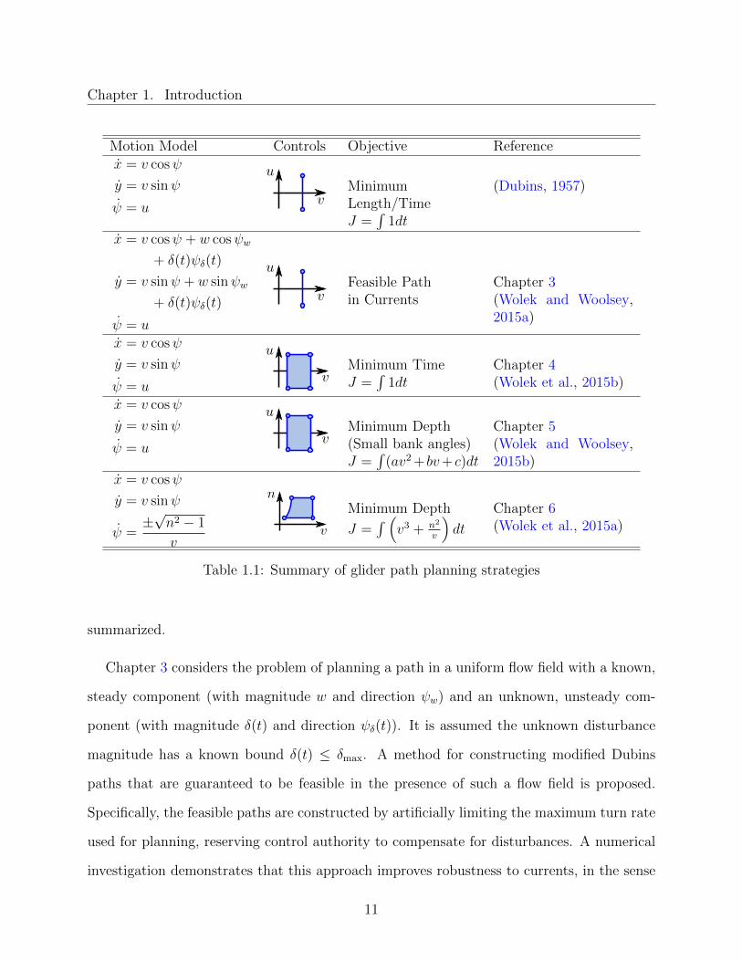
faced by shallow water gliders. See Table 1.1 for a comparison of Dubins motion model,
control constraint set, and cost function to the series of problems considered here. In the
motion models of Table 1.1, the planar position is (x, y) and the heading is ψ. The control
inputs are: speed v, turn rate u, and load factor n (when applicable). The Lagrange type
cost functional is J . The first row of Table 1.1 summarizes Dubins problem. In this case,
the speed is fixed and the turn rate controls are bounded symmetrically about zero. For a
fixed speed, minimum length and minimum time paths are equivalent.
Chapter 2 reviews the main mathematical tools used throughout this work. The necessary
conditions for an optimal control, provided by the Minimum Principle, are discussed. A
geometric interpretation of the min-H operation (of the Minimum Principle where H is the
Hamiltonian) is reviewed. An analytical approach for applying the min-H operation over a
control constraint set defined by inequality constraints is also outlined. An existence theorem
for optimal controls is reviewed. Details of Dubins (1957) path planning approach are briefly
10
Chapter 1. Introduction
Motion Model Controls Objective Referencex = v cosψ
y = v sinψ
ψ = u
MinimumLength/TimeJ =
∫1dt
(Dubins, 1957)
x = v cosψ + w cosψw
+ δ(t)ψδ(t)
y = v sinψ + w sinψw
+ δ(t)ψδ(t)
ψ = u
Feasible Pathin Currents
Chapter 3(Wolek and Woolsey,2015a)
x = v cosψ
y = v sinψ
ψ = u
Minimum TimeJ =
∫1dt
Chapter 4(Wolek et al., 2015b)
x = v cosψ
y = v sinψ
ψ = u
Minimum Depth(Small bank angles)J =
∫(av2 + bv+c)dt
Chapter 5(Wolek and Woolsey,2015b)
x = v cosψ
y = v sinψ
ψ =±√n2 − 1
v
Minimum Depth
J =∫ (
v3 + n2
v
)dt
Chapter 6(Wolek et al., 2015a)
Table 1.1: Summary of glider path planning strategies
summarized.
Chapter 3 considers the problem of planning a path in a uniform flow field with a known,
steady component (with magnitude w and direction ψw) and an unknown, unsteady com-
ponent (with magnitude δ(t) and direction ψδ(t)). It is assumed the unknown disturbance
magnitude has a known bound δ(t) ≤ δmax. A method for constructing modified Dubins
paths that are guaranteed to be feasible in the presence of such a flow field is proposed.
Specifically, the feasible paths are constructed by artificially limiting the maximum turn rate
used for planning, reserving control authority to compensate for disturbances. A numerical
investigation demonstrates that this approach improves robustness to currents, in the sense
11

Chapter 1. Introduction
that final cross track error is minimized when the paths are tracked with a standard path
following algorithm.
Chapter 4 revisits the Dubins path planning problem and relaxes the fixed speed con-
straint. A minimum-time path planning problem is formulated where the speed is strictly
positive, ranging from a lower to an upper limit, and the turn rate limits are symmetric
about zero. The Minimum Principle is used to characterize the extremal controls and, using
additional geometric arguments, a finite and sufficient set of candidate optimal controls is
derived. It is found that, in addition to straight and maximum rate turning segments at max-
imum speed, minimum-time paths may include “cornering turns” at the minimum forward
speed and the maximum turn rate. A procedure is proposed for solving the path synthesis
problem of constructing the minimum-time path between two “oriented points” in the plane.
Chapter 5 considers the optimal control problem of minimizing the depth change of a
glider maneuvering in still water to a nearby position and heading angle. Again, a Dubins-
like motion model with variable speed controls is considered. The sink rate of the glider is
assumed to be a quadratic function of the forward speed: av2 + bv + c, approximating the
“glide polar”. This approximation is valid for shallow bank angles. The extremal controls
are characterized and a finite and sufficient set of candidate optimal controls is derived. The
extremal paths are shown to consist of (i) straight line segments flown at the glider’s “best
glide” speed and (ii) maximum rate turns with either: (a) a heading dependent speed input,
(b) the stall speed, or (c) the minimum sink speed. A synthesis procedure is proposed to
solve for the minimum depth path.
Chapter 6 revisits the minimum depth problem (of Chapter 5) and relaxes the shallow
bank angle restriction. A more realistic physics-based model is proposed in which the turn
rate and sink rate are coupled with the speed. The problem is formulated with speed and load
factor controls. (Load factor n is the ratio of the lift to weight. Here this corresponds to a
12
Chapter 1. Introduction
given bank angle.) The extremal controls are characterized using the Minimum Principle. A
parametric study of various adjoint variable conditions gives insight regarding the extremal
control trajectories. The path synthesis problem of joining given boundary conditions is
formulated and solved using a commercially available optimal control solver to illustrate the
analytical results.
Chapter 7 discusses the design, fabrication and testing of an underwater glider. The
glider has a novel pneumatic buoyancy engine that allows for large, rapid buoyancy changes
and a fast cylindrical moving mass mechanism that generates large pitch and roll moments
to improve attitude control. This moving mass actuator gives the glider the ability to roll
over between dives and permits the use of cambered hydrofoils for improved hydrodynamic
efficiency or dihedral for improved turning performance.
Chapter 8 summarizes the contributions of this work.
13
Chapter 2
Mathematical Preliminaries
2.1 An Optimal Control Problem
The optimal control problems consider in this work take the following form (with notation
adapted from (Burns, 2013)):
Consider the control system
x(t) = ~f(x(t),u(t)), t > t0 , (2.1)
where x(t) ∈ Rn is the state, u(t) ∈ Rm is the control, ~f : Rn × Rm → Rn is a smooth
function, and t0 ∈ R is the initial time (which we will generally take to be zero). Let
PWC(t0, t1;Rn) denote the set of n-dimensional vectors of real-valued piecewise continuous
functions on the interval [t0, t1]. At a given time t ∈ [t0, t1], the available inputs u(t) are
confined to the control constraint set Ω ⊆ Rm. Define the initial set X0 ⊆ Rn and terminal
set X1 ⊆ Rn. In this work we will consider problems in which the final time t1 ∈ R is free.
14

Chapter 2. Mathematical Preliminaries
The initial conditions are given by
x(t0) = x0 ∈ X0 . (2.2)
The set of admissible, piecewise continuous controls that satisfy the boundary conditions is
Θ =
u(·) ∈ PWC(t0, t1;Rm) : u(t) ∈ Ω except at a finite
number of points, and x(·) is a solution to
the initial value problem (2.1)-(2.2) satisfying x(t1) = x1 ∈ X1.
.
The cost functional is
J(u(·)) =
∫ t1
t0
f0(x(τ),u(τ))dτ . (2.3)
where f0 : Rn×Rm → R is a smooth function that takes an admissible control u(·) (and the
associated solution x(·), with (2.2)) and assigns a scalar cost, J(u(·)) : u(·) ∈ Θ→ R.
The problem is to find an optimal control u∗(·) ∈ Θ and x∗(t0) = x∗0 ∈ X0, where x∗(·) is
a solution to the initial value problem (2.1)-(2.2) with t∗1 > t0, such that J(u∗(·)) ≤ J(u(·))
for all u(·) ∈ Θ.
Note that in the above formulation a superscript asterisk refers to an optimal quantity.
When the meaning is clear from context this notation is suppressed for brevity. We also use
shorthand variables (e.g. u) to refer to a function (e.g. u(·) ∈ Θ) or the value of a function
at a point (e.g. u(t) ∈ Ω).
15

Chapter 2. Mathematical Preliminaries
2.2 Pontryagin’s Minimum Principle
The main tool for analysis of the nonlinear optimal control problems in this dissertation is
Pontryagin’s Minimum Principle. The Minimum Principle gives necessary conditions for an
optimal control. A complete derivation and discussion of the Minimum Principle can be
found in standard optimal control texts; see (Pontryagin et al., 1962; Lee and Markus, 1967;
Leitmann, 1981). The remainder of this section presents the Minimum Principle, in a form
adapted from (Burns, 2013).
Define the cost variable
x0(t1) =
∫ t1
t0
f0(x(τ),u(τ))dτ ,
the augmented state
x =
x0
x
,
and the augmented vector field
f(x,u) =
f0(x,u)
~f(x,u)
,
such that ˙x = f(x,u). (In general, x0 does not appear in f explicitly so f(x,u) is equivalent
to f(x,u).) Further, define the adjoint vector (sometimes called the co-state vector)
η(t) = (η0(t), η1(t), η2(t), · · · , ηn(t))T =
η0(t)
~η(t)
,
16

Chapter 2. Mathematical Preliminaries
and the variational Hamiltonian
H(η(t), x(t),u(t)) = η0f0(x,u) + 〈~η, ~f(x,u)〉
= η0f0(x,u) +n∑i=1
ηifi(x,u) .
With this notation we may now state the Minimum Principle.
Theorem 2.2.1 (Minimum Principle). If u∗(·) minimizes J(u(·)) on the set of admissible
controls Θ with optimal response x∗(·) satisfying x∗(t0) = x∗0 ∈ X0 and x∗(t∗1) = x∗1 ∈ X1 at
time t∗1 > t0, then:
1. there exists a non-trivial solution
η(t) = (η0(t), η1(t), η2(t), · · · , ηn(t))T =
η0(t)
~η(t)
6= 0 (2.4)
to the augmented adjoint equation
d
dtη(t) = −
(∂H
∂x
)T∣∣∣∣∣x=x∗, u=u∗
(2.5)
with
η0(t) ≡ η0 a constant satisfying η0 ≥ 0 ,
2. the optimal control u∗(·) minimizes the Hamiltonian evaluated along the optimal re-
sponse x∗(·) and the optimal adjoint solution η(·), such that
minu∈Ω
H(η(t), x∗(t),u) = H(η(t), x∗(t),u∗(t)), (2.6)
17
Chapter 2. Mathematical Preliminaries
3. and for all t ∈ [t0, t∗1],
minu∈Ω
H(η(t), x∗(t),u) ≡ 0 . (2.7)
4. Also if X0 ⊆ Rn and X1 ⊆ Rn are manifolds with tangent spaces T0 and T1 at x∗(t0) =
x∗0 ∈ X0 and x∗(t∗1) = x∗1 ∈ X1, respectively, then η(t) = (η0(t), ~η(t))T can be selected
to satisfy the transversality conditions
~η(t0) ⊥ T0 , (2.8)
and
~η(t∗1) ⊥ T1 . (2.9)
For the problems considered in this work the initial and terminal sets, X0 and X1 respec-
tively, are singleton. Thus the tangent spaces, T0 and T1 respectively, are both equal to
the zero vector and the transversality conditions (2.8)-(2.9) are always satisfied. Thus they
provide no additional information, but they are stated here for completeness.
2.3 Indirect and Direct Methods
There are two main methods for solving optimal control problems: indirect and direct meth-
ods. Using the indirect method, the Minimum Principle is applied and this leads to a
two-point boundary-value (TPBV) problem. A solution (x∗(·), η(·),u∗(·)) that satisfies the
necessary conditions of the Minimum Principle is called an extremal. In some cases the ex-
tremals satisfying the boundary conditions may be derived analytically. Additional analysis
of the necessary conditions, under various adjoint variable conditions, may reveal the struc-
18

Chapter 2. Mathematical Preliminaries
ture of the optimal control. The following list sketches the indirect approach used for the
problems considered in this dissertation:
• Existence of an optimal control.
The existence theorem discussed in Section 2.6 is used to show that the optimal control
problem is well posed.
• Extremal controls under various adjoint vector conditions.
The necessary conditions of the Minimum Principle are applied to the problem. The
min-H operation gives the extremal controls as a function of the adjoint vector: u∗(η).
The hodograph and/or the Karush-Kuhn-Tucker conditions are useful for this analysis,
as described in Sections 2.4 and 2.5, respectively. The extremal controls u∗(η) are
grouped into k ∈ Z distinct families: Fi where i ∈ 1, · · · , k. Each extremal family
Fi corresponds to a unique adjoint vector conditions and a locus of extremal controls
in Ω. The set F = Fiki=1 contains all of the extremal families.
• Determining admissible extremal sequences.
As the adjoint vector evolves, the extremal control may transition from one family
to another. Studying the adjoint differential equation (2.5), and the state equation
(2.1), with u∗(η), one may conclude which extremal families may join each other in
succession (i.e. which extremal sequences are admissible). (For example, to ensure that
the adjoint vector evolves continuously one may find that only certain families Fi may
succeed each other.) This type of reasoning leads to the definition of Γ, a (possibly)
infinite set of all admissible sequences of extremals. (At this point in the analysis, Γ
may contain many spurious sequences that remain to be identified and rejected.)
• Parameterizing extremal sequences.
Sequences of extremals are parametrized by a finite dimensional vector p ∈ Rnp . For
19

Chapter 2. Mathematical Preliminaries
example, the parameter vector may indicate the duration of particular extremal arcs in
the sequence. Restricting the boundary conditions, the parameter vector p can also be
restricted such that p ∈ P ⊂ Rnp . For example, if the problem is restricted to endpoints
within a certain distance of the origin, then one may construct a conservative bound
for the maximum duration of extremal arcs defined by p.
• Deriving sub-optimality conditions for extremal sequences.
While Γ contains admissible extremal sequences, many of these may be spurious can-
didates that never correspond to an optimal control. One may show that certain
sequences are sub-optimal (i.e. they do not minimize the cost functional). For exam-
ple, if a certain extremal sequence can always be replaced by an alternate, lower cost,
control that meets the boundary conditions, then it is clear that the extremal sequence
under consideration is not a minimizer. Note that this alternate control need not nec-
essarily be itself an extremal since it only serves to show sub-optimality by comparison.
Such sub-optimality conditions may either rule out a given extremal sequence entirely
(if they hold in general), or they may restrict the domain P for a particular sequence
(if they only hold under some conditions on p).
• A finite and sufficient set of candidate optimal controls.
Any sequence in Γ that is equal to, or contains in part, a sub-optimal sequence is itself
sub-optimal. Spurious solutions may be eliminated from Γ using the sub-optimality
conditions discussed above. If enough sub-optimality conditions are identified, then
Γ may be reduced from a (possibly) infinite set of candidate extremal sequences to a
finite set of candidate extremal sequences. However, reducing Γ to a finite set does
not imply it is minimal (i.e. Γ may still contain spurious candidates that correspond
to sub-optimality conditions not used in the aforementioned reduction). With this
approach, Γ becomes the set of all candidate extremals sequences that satisfy the
20
Chapter 2. Mathematical Preliminaries
necessary conditions of the Minimum Principle without violating the identified sub-
optimality conditions. Having shown that an optimal control exists, it follows that Γ
contains the globally optimal control. In path planning, “a set which always contains
the optimal path” is sometimes referred to as sufficient set (Reeds and Shepp, 1990).
A primary goal in this dissertation is to derive a finite and sufficient set Γ for the
problems considered herein.
• Identifying the (lowest cost) optimal control.
The task then becomes to identify the sequence in the (finite) set Γ and the (finite
dimensional) parameter vector p ∈ P that gives the globally optimal control. One
approach is to identify all of the solutions in Γ that satisfy the boundary conditions.
Let p′ ∈ P refer to a parameter vector that satisfies the boundary conditions for a
given sequence in Γ. Then by enumerating all p′, for all candidates in Γ, and compar-
ing the costs of each of these solutions, the lowest cost solution will give the globally
optimal control. In practice, however, the difficulty is in identifying all p′. If for a
given candidate in Γ the solutions p′ ∈ P are isolated points in P then finding p′ is
equivalent to root finding. For simple cases these solutions may be derived analyti-
cally (as shown in (Tang et al., 1998) for the Dubins problem). Otherwise one may
employ a numerical root finding routine (as shown in (Techy and Woolsey, 2009) for
the “convected” Dubins problem in known, steady winds). If for a given candidate
in Γ there are continuous spaces P ′ of solutions p′ ∈ P ′ ⊂ P then an optimization
routine may be used to identify the “locally” optimal parameter vector p∗ ∈ P ′. An
algorithm may be constructed to numerically perform the aforementioned root solving
and finite-dimensional optimization routines. However, there is no guarantee that all
solutions (p′ or p∗, as applicable) will be found numerically. Thus, it cannot be claimed
that the lowest cost control obtained with such a procedure is globally optimal.
21

Chapter 2. Mathematical Preliminaries
This approach is only tractable for some relatively simple, low-dimensional problems, such
as those considered in this work. For more complex systems, one generally seeks to solve the
TBVP numerically (for example, using shooting or collocation methods). Alternatively, the
direct method is used to discretize the infinite dimensional control in some manner (e.g. by
parameterizing the controls) and the optimal control problem is then transcribed into the
form of a nonlinear programming problem.
2.4 The Hodograph
Using the indirect method, a useful tool to study the necessary conditions is the hodograph.
The hodograph, or velocity set, provides a way to interpret minimizing the Hamiltonian (the
min-H operation (2.6)) geometrically. This method is particularly useful when the controls
only appear in a few of the state-rate equations and the hodograph can be graphically
depicted. Cliff et al. (1993) discuss the use of the hodograph as a tool in optimal control.
The hodograph for a fixed state x is the image of Ω under the vector field f(x,u)
Dx ≡ z|z = f(x,u) where u ∈ Ω .
In other words, the hodograph gives the set of cost and state rates attainable at a given
state x for all controls u in the control constraint set Ω. The variational Hamiltonian may
22
Chapter 2. Mathematical Preliminaries
be expressed as the inner product
H(η, x,u) = η0f0(x,u) + 〈~η, ~f(x,u)〉
=
⟨ η0
~η
,
f0(x,u)
~f(x,u)
⟩
=⟨η, f(x,u)
⟩.
This is the inner product between an augmented adjoint vector η and a vector f(x,u) in
the hodograph set Dx. The locus of augmented state-rate vectors fperp(x,u) ∈ η⊥ forms
a hyperplane where H = 0. If this hyperplane is translated by a fixed vector a, then by the
linearity of the inner product the Hamiltonian is constant along the translated subspace
H(η, x,u) =⟨η, fperp(x,u) + a
⟩=⟨η, fperp(x,u)
⟩+ 〈η,a〉
= 〈η,a〉 ,
where 〈η,a〉 = c a constant. Thus to perform the min-H operation for a fixed state x,
and a fixed adjoint vector η , one seeks the translated subspace (parallel to η⊥) that
minimizes H = c and that contains a point (or points) in the hodograph set. It is clear
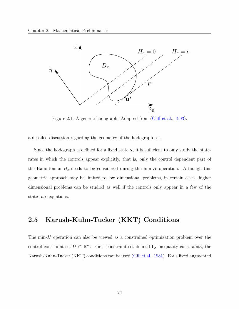
that this will occur on the boundary of the hodograph set. The hyperplane defined at that
minimizing point(s) is called the separating plane P , and the side of P that has no points
in Dx is the side where H is smaller than it is for any other point in Dx. This is illustrated
in Figure 2.1. Note that P may not be unique for a given point on the boundary of the
hodograph. (For example the point may correspond to a corner that has infinitely many
separating planes, each corresponding to a unique adjoint vector.) See (Cliff et al., 1993) for
23
Chapter 2. Mathematical Preliminaries
Figure 2.1: A generic hodograph. Adapted from (Cliff et al., 1993).
a detailed discussion regarding the geometry of the hodograph set.
Since the hodograph is defined for a fixed state x, it is sufficient to only study the state-
rates in which the controls appear explicitly, that is, only the control dependent part of
the Hamiltonian Hc needs to be considered during the min-H operation. Although this
geometric approach may be limited to low dimensional problems, in certain cases, higher
dimensional problems can be studied as well if the controls only appear in a few of the
state-rate equations.
2.5 Karush-Kuhn-Tucker (KKT) Conditions
The min-H operation can also be viewed as a constrained optimization problem over the
control constraint set Ω ⊂ Rm. For a constraint set defined by inequality constraints, the
Karush-Kuhn-Tucker (KKT) conditions can be used (Gill et al., 1981). For a fixed augmented
24
Chapter 2. Mathematical Preliminaries
state x∗ and adjoint vector η define H(u) = H(η(t), x∗(t),u) and consider the problem
minimize H(u)
subject to : gi(u) ≤ 0 ,
where i = 1, · · · ,m, and gi(u) are the inequality constraints that define the control constraint
set Ω. Define the system Lagrangian
L(µ,u) = H(u) +m∑j=1
µigi(u) ,
where the Lagrange multipliers µ = [µ1, µ2, · · · , µm]T are sometimes called Valentine mul-
tipliers, after F.A. Valentine who studied such inequality constraints in the Calculus of
Variations setting (Valentine, 1937). Then the first-order necessary conditions for optimality
is
∇H(u) = 0 ,
where µ1, µ2, · · · , µm ≥ 0. When the i-th constraint becomes active µi > 0; otherwise µi = 0.
A convenient way to evaluate the KKT conditions is to study the problem first along the
boundary of Ω considering each constraint (or combinations of constraints as appropriate)
and then to consider the case when no constraints are active on the interior of Ω. Note that
the hodograph and the KKT conditions characterize the extremal controls for a fixed x∗
and η. To determine how the controls change in time we must study the adjoint differential
equation (2.5).
25

Chapter 2. Mathematical Preliminaries
2.6 An Existence Theorem for Optimal Controls
Prior to applying the necessary conditions of the Minimum Principle it is important to
ensure, if possible, that an optimal control exists for the problem being considered. The
danger of assuming that a solution exists is illustrated by Perron’s Paradox wherein one
may construct a seemingly valid proof that the largest integer is N = 1. For a discussion
of Perron’s Paradox and the assumptions made in deriving the necessary conditions in the
Calculus of Variations see (Young, 1969).
The following Theorem is specialized from the more general result in (Lee and Markus
(1967), Chapter 4, Theorem 4) and may be used to determine the existence of an optimal
control for the problems considered in this dissertation.
Theorem 2.6.1 (Existence of an Optimal Control). If the optimal control problem
discussed in Section 2.1 has the following properties:
1. the initial and terminal sets, X0 and X1 respectively, are fixed points in Rn,
2. the control constraint set Ω ⊆ Rm is a fixed, nonempty, compact set,
3. there are no state constraints
4. the set of admissible controllers is u(·) ∈ Θ,
5. the cost functional integrand f0(x,u) is smooth
6. the system (2.1) is controllable,
7. and the hodograph set Dx is convex for each x,
then there exists an optimal control u∗(·) ∈ Θ that minimizes J(u(·)) for all u(·) ∈ Θ.
26

Chapter 2. Mathematical Preliminaries
Therefore if the hodograph is nonconvex there is no guarantee that an optimal control
exists. In such cases, the problem may be “relaxed” by reformulating it such that the hodo-
graph of the relaxed problem is the convex hull of the hodograph of the original problem. A
solution to the relaxed problem is a solution to the original problem if the associated state-
rates (and controls) are admissible in both formulations. See (Cliff et al., 1993) for a detailed
discussion of the relevance of hodograph convexity to the existence of an optimal control.
The above Theorem 2.6.1 uses the notion of controllability, which is defined as follows:
Definition 2.6.1 (Controllability). The system (2.1) is said to be controllable if there
exists a piecewise continuous control u(·) ∈ PWC(t0, t1;Rm) : u(t) ∈ Ω ⊂ Rm and resulting
solution x(·) to the initial value problem (2.1)-(2.2) such that the terminal state x(t1) = x1 ∈
X1 is reached in finite time t1 − t0.
For a detailed discussion of controllability for nonlinear systems see (Bloch, 2003; Bullo
and Lewis, 2004).
2.7 Dubins Path Planning
Much of the work in this dissertation is an extension of Dubins path planning problem. In
the following we briefly review this path planning approach.
Consider a vehicle that moves in an inertial, horizontal plane at a constant forward speed
v and in some direction ψ relative to a reference frame FI fixed in the plane. For the moment,
assume that there are no disturbances acting on the vehicle. The vehicle’s position is given
by the pair (x, y). The input is the turn rate u, which is symmetrically bounded. A turn at
maximum rate corresponds to a circular path of minimum radius R0. The input constraint
27

Chapter 2. Mathematical Preliminaries
may be expressed in terms of this minimum turn radius and the vehicle’s speed:
|u| ≤ v
R0
.
The equations of motion, which define the standard Dubins car model, are
x(t)
y(t)
ψ(t)
=
v cosψ(t)
v sinψ(t)
u(t)
. (2.10)
In his seminal work, Dubins (1957) considered the problem of finding paths of minimum
length and bounded curvature that connect two points in the plane with given initial and
final tangents. (This is equivalent to the problem of finding the minimum length path
for the system (2.10) starting from the origin with heading ψ0 = 0 to a terminal state x1 =
(x1 y1 ψ1)T. This latter problem was solved by Sussmann and Tang (1991) and Boissonnat
et al. (1992) using optimal control techniques. Note that for a fixed speed, minimum length
and minimum time paths are equivalent.) Specifically, Dubins used geometric arguments to
show that the minimum length path is a member of the set
LSL,LSR,RSL,RSR,LRL,RLR . (2.11)
Each letter in a sequence listed above refers to the sense of a path segment: L for a maximum
rate left turn, R for a maximum-rate right turn, and S for a straight segment. Because the
control constraints are symmetric, the radius R0 of a maximum-rate turn is the same whether
the turn is to the left or the right. To illustrate this result, consider Figure 2.2 in which
the candidate paths to a given endpoint x1 are shown. (Note that in Figure 2.2 the planar
positions are normalized by the minimum turn radius such that x = x/R0 and y = y/R0.)
28

Chapter 2. Mathematical Preliminaries
−6 −4 −2 0 2−3
−2
−1
0
1
2
3
4
5
(a) x1 = (−3 2 3π/2)T
−2 −1 0 1 2 3
−2
−1
0
1
2
3
(b) x1 = (1 1 π)T
Figure 2.2: Candidate Dubins paths for a given endpoint x1
For a given endpoint, only some members of the set (2.11) will be feasible. For example, in
Figure 2.2(a) the endpoint is far away and cannot be reached by a sequence of three turns
alone; only the candidates containing an S segment are feasible. Whereas in Figure 2.2(b)
the endpoint is closer to the origin and can be reached by a turn-turn-turn (e.g. RLR)
candidate. To identify the optimal Dubins path, one may construct all feasible candidates
(for example, using the method proposed by Tang et al. (1998) or Anisi (2003)) and compare
their costs. Alternativley, one may use the result from (Bui et al., 1994) in which the plane
is partitioned, for a given final heading ψ1, into regions where the optimal path type(s) is
known. One then simply checks the “partition” corresponding to a given endpoint x1 to
obtain the optimal path type(s).
29

Chapter 3
Feasible Paths in Unknown, Unsteady
Currents
3.1 Introduction
Underwater gliders operating in shallow waters must often contend with complex and dy-
namic currents that are either only approximately modeled or completely unknown. Reliable
glider operations require a path planning strategy that is robust to such disturbances. Recall
that a time-optimal Dubins path consists of maximum rate turns and straight line segments.
However, a Dubins path that is constructed using the true maximum turn rate cannot be
tracked in the presence of disturbances, because feedback commands may exceed the turn
rate limit. If there is sufficient control authority, and the disturbances are perfectly known
(whether steady (McGee and Hedrick, 2007; Techy and Woolsey, 2009; Bakolas and Tsio-
tras, 2010) or unsteady (McNeely et al., 2007)), then minimum time trajectories to the goal
state can be planned that account for these disturbances explicitly. In general, though, dis-
turbances are unknown and unavailable for planning and control purposes. One approach
30
Chapter 3. Feasible Paths in Unknown, Unsteady Currents
to dealing with uncertain disturbances is to dispense with planning altogether and to use
feedback control to drive the system toward a desired end goal. In (Anderson et al., 2013),
for example, an optimal control law is presented that drives the vehicle to a target set (with
a free final course angle) in the presence of a stochastically varying wind. In some applica-
tions, however, such as directional sensing or vehicle recovery operations, attaining a desired
position with a specific course angle may be important.
Here the Dubins path planning method is modified to construct sub-optimal paths that
remain feasible in the presence of a bounded, unsteady disturbance. The path is planned
using an artificially reduced “maximum” turn rate that is a function of the (known) upper
bound on the disturbance magnitude. Though the resulting path is longer, it could be tracked
by the vehicle if the disturbance were known. For unknown disturbances, the reserve control
authority enables a path following algorithm to force convergence to the desired path. The
following is based on the work in (Wolek and Woolsey, 2012, 2015a).
3.2 Problem Formulation
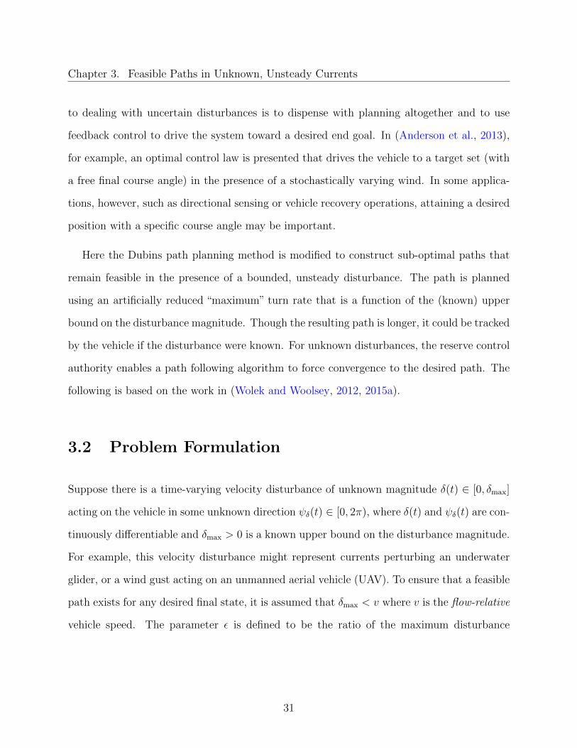
Suppose there is a time-varying velocity disturbance of unknown magnitude δ(t) ∈ [0, δmax]
acting on the vehicle in some unknown direction ψδ(t) ∈ [0, 2π), where δ(t) and ψδ(t) are con-
tinuously differentiable and δmax > 0 is a known upper bound on the disturbance magnitude.
For example, this velocity disturbance might represent currents perturbing an underwater
glider, or a wind gust acting on an unmanned aerial vehicle (UAV). To ensure that a feasible
path exists for any desired final state, it is assumed that δmax < v where v is the flow-relative
vehicle speed. The parameter ε is defined to be the ratio of the maximum disturbance
31

Chapter 3. Feasible Paths in Unknown, Unsteady Currents
magnitude to the vehicle’s flow-relative speed:
ε =δmax
v< 1 . (3.1)
Incorporating this disturbance, the system (2.10) becomes
x(t)
y(t)
ψ(t)
=
v cosψ(t) + δ(t) cosψδ(t)
v sinψ(t) + δ(t) sinψδ(t)
u(t)
. (3.2)
One may construct a path that is feasible for the system (3.2) by constructing a Dubins path
for the system (2.10) using a “feasible turn radius” R′0 which is larger than R0, but which
affords the vehicle more turn rate authority to compensate for the disturbance. As shown in
Appendix A, given δ(t) ≤ δmax and ψδ(t), a Dubins path planned using the turn radius
R′0 = R0(1 + ε)2 , (3.3)
is feasible for the system (3.2), meaning there exists a control u∗(t) for which the vehicle
perfectly follows the desired path. While u∗(t) exists, determining this input requires exact
knowledge of the disturbance. Advanced sensors may enable such feedforward disturbance
rejection, but it is more common that only the vehicle’s state (position and course angle)
is directly measured. In this case, one may use feedback control to diminish the effect of
disturbances.
The result (3.3) is closely related to Lemma 6 in (Peterson and Paley, 2011) wherein the
maximum turn rate required to maintain a fixed circular orbit in a known time-invariant
flow field is derived. This maximum turn rate corresponds to the feasible turn radius R′0 as
defined here. However, the present work demonstrates that R′0 holds for a more general case,
32

Chapter 3. Feasible Paths in Unknown, Unsteady Currents
−6 −4 −2 0 2 4 6−6
−4
−2
0
2
4
6
x
y
LSR
RLR/LRL
RLR/LRL
RSR/LSL
RSL
(a) P0
−6 −4 −2 0 2 4 6−6
−4
−2
0
2
4
6
x
y LRL
RLR
RSL
LSR
RSL
LSL
RSR
LSR
(b) P2π/3
−6 −4 −2 0 2 4 6−6
−4
−2
0
2
4
6
x
y
LSL
RLR
LRL
RSR
LSR
RSLLSR
RSL
(c) Pπ
Figure 3.1: Partitions of the configuration space for final course angles ψ1 = 0, 2π/3and π, respectively
where only an upper bound on the disturbance magnitude is known and the flow field is
assumed to be time-varying and continuously differentiable. In the following, the convention
used in related works is adopted and the path planning problem is discussed in terms of
aircraft motion in winds, recognizing the results also apply to underwater gliders in currents.
If there is a known, steady, uniform wind in addition to the random disturbances, one may
account for this wind explicitly. Several methods have been developed to plan time-optimal
paths in known, steady winds (only) (McGee and Hedrick, 2007; Techy and Woolsey, 2009;
Bakolas and Tsiotras, 2010). In these cases, the resulting optimal path always consists of
trochoids and straight segments in the fixed, inertial frame FI . Equivalently, it consists of
circular arcs and straight segments in an air-relative frame FA that moves with the mean
wind velocity. As shown in Appendix A, the result (3.3) extends to the case where there is
a known, steady, uniform wind and a unknown, unsteady disturbance (with a known upper
bound), under the additional restriction that w + δmax < v, where w is the steady, mean
wind speed.
33

Chapter 3. Feasible Paths in Unknown, Unsteady Currents
x
y
−6 −4 −2 0 2 4 6−6
−4
−2
0
2
4
6
1
2
3
4
5
(a) T (x1, y1, 0, 0.25)
xy
−6 −4 −2 0 2 4 6−6
−4
−2
0
2
4
6
1
2
3
4
5
(b) T (x1, y1, 2π/3, 0.25)
x
y
−6 −4 −2 0 2 4 6−6
−4
−2
0
2
4
6
1
2
3
4
5
(c) T (x1, y1, π, 0.25)
Figure 3.2: Contour maps of the ratio of optimal path lengths planned using R′0 andR0
3.3 Tradeoff Between Path Length and Path Feasibility
One may assume without loss of generality that the vehicle begins at the state x0 =
(0 0 0)T , so that the path planning problem is completely defined by the desired final
state x1 = (x1 y1 ψ1)T . Since optimal paths may be parameterized by the final position
(x1 and y1) and the final course angle ψ1, one may construct a diagram, for a given value
of ψ1, which identifies regions of the (x, y) plane in which minimum time paths from the
origin to a given final point, with the final course angle ψ1, are of a given type; see (Bui
et al., 1994; Boissonnat and Bui, 1994). One may thus associate a “partition” Pψ with each
final course angle ψ1 ∈ [0, π], recognizing that the partition P−ψ is the reflection of Pψ about
the x axis. Figures 3.1(a), 3.1(b) and 3.1(c) illustrate three such partitions for final course
angles ψ1 = 0, 2π/3 and π, respectively. The unit of length for the axes is the minimum
turn radius R0, so that points in the plane are given in normalized position coordinates
(x, y) = (x/R0, y/R0).
For a given final course angle ψ1 and a final position (x1, y1), one may compare the length
of the optimal Dubins path (planned with R0) to that of the sub-optimal feasible Dubins
path (planned with R′0) by taking the ratio of the path lengths. Referring to the length of
34

Chapter 3. Feasible Paths in Unknown, Unsteady Currents
each of these paths as doptimal(x1, y1, ψ1) and dfeasible(x1, y1, ψ1, ε) respectively, the ratio
T (x1, y1, ψ1, ε) =dfeasible
doptimal
gives a measure of the sub-optimality of the feasible path. A large value of T indicates
that allowing for a disturbance by using the planning radius R′0 significantly increases the
path length. (Alternatively, one might consider another measure of sub-optimality, such
as the ratio of transit times of the feasible to optimal path. However, the time-varying
velocity disturbance is unknown and therefore the time to traverse the feasible path is not
well defined. Thus this measure of sub-optimality is not used in this work. Note that in the
presence of a wind-field minimum length and minimum time paths are no longer equivalent.)
Contours of the“tradespace”T (x1, y1, ψ1, ε) may be generated by synthesizing the optimal
paths using R0 and R′0 for a grid of points around the origin. The examples in Figures 3.2(a),
3.2(b) and 3.2(c) illustrate this tradespace for ε = 0.25 and for final course angles ψ1 = 0, 2π/3
and π, respectively. In each figure the“thermal scale”representing T (x1, y1, ψ1, ε) is truncated
at 5 for clarity and the contour lines are drawn in intervals of 0.2.
Figures 3.2(a), 3.2(b) and 3.2(c) indicate that, for points far from the origin, the relative
cost of using a larger turn radius to plan the Dubins path is small. However, both figures have
regions, especially within 4 turn radii R0 of the origin, where there is a dramatic increase in
relative path length. This issue can be understood by referring to the partitions in Figure 3.1.
Consider two paths, with the same final heading ψ1, that are planned to the same terminal
point (x1, y1). Assume one path is planned using R0 as the planning radius and another
using R′0 > R0. The path planned using R0 maps to the point 1R0
(x1, y1) in the partition,
and the path planned with R′0 maps to the point 1R′0
(x1, y1), which is nearer the origin. If
these two points map to different regions within the partition then the qualitative type of
35

Chapter 3. Feasible Paths in Unknown, Unsteady Currents
each path will be different, possibly leading to a large path length ratio T (x1, y1, ψ1, ε).
3.4 Path Following Performance
To follow a Dubins path planned with the feasible turn radius R′0 requires perfect knowledge
of the disturbances. Since accurate ambient flow measurements are typically unavailable,
a feedback control system based on position and attitude measurements is typically used
instead. Well-designed feedback control can enhance robustness to model uncertainty and
disturbances, provided there is sufficient control authority to execute the control commands.
The point of this work is to suggest a path planning strategy that produces sub-optimal
paths which can still be followed in the presence of unknown disturbances. Specifically, it is
suggested that Dubins paths planned using the feasible turn radius R′0 will be “robust” to
unknown disturbances, in the sense that these paths can be closely followed in spite of these
disturbances. In this section, this hypothesis is investigated numerically.
In this numerical investigation, a UAV is modeled as a Dubins car moving at air-relative
speed v = 20 m/s and with a turn rate limit |u| ≤ 0.3 rad/s. For closed-loop path following,
the lookahead-based guidance law for regularly parameterized paths described in (Breivik
and Fossen, 2008) is used. The course commands generated by the algorithm in (Breivik
and Fossen, 2008) are tracked with a bang-bang turn rate controller; the control parameters
are chosen heuristically to give reasonable performance over a wide range of wind conditions
and turn radii. This path following algorithm is illustrated in Figures 3.3(a) and 3.3(b) for
two sample endpoints in a steady, uniform wind blowing in the positive x direction (with
ε = 0.25). In these figures, two paths are planned to each state x1; one path is planned
using the true minimum turn radius R0 (dashed line) and the other using R′0 (dashed-dotted
line). The UAV’s motion is simulated (solid line) using the guidance law from (Breivik and
36

Chapter 3. Feasible Paths in Unknown, Unsteady Currents
Fossen, 2008) to follow a given path. It seems clear from these figures that path following
performance is improved for the paths planned using the feasible turn radius R′0, rather than
R0. For both examples, the vehicle more closely follows the path planned using R′0, resulting
in greater accuracy for the endpoint and the final course angle. The tradeoff, of course, is the
increase in path length. To study the effect of varying the turn radius used in path planning
on the path following performance, a Monte Carlo simulation study was conducted.
0 1 2 3 4
0
1
2
3
x
y
R0
R0‘
END
START
(a) x1 = [3 3 2π/3]T
−2 0 2
−3
−2
−1
0
1
2
3
4
x
y
R0
R0‘
START
END
(b) x1 = [1 2 0]T
Figure 3.3: Comparison of closed-loop path following performance (solid lines) for pathsplanned to the state x1 using turn radii R0 (dashed line) and R′0 (dashed-dotted line)
A Monte Carlo simulation was used to compare the path following performance for various
turn radii Rplan ≥ R0 used in path planning. The aim of this simulation was to illustrate the
changes in path following performance for incrementally increasing Rplan and, in particular,
to show the effect of choosing Rplan = R′0. A number of measures could be used to assess
path following performance for these different choices of planning radius. One might measure
overall tracking performance, for example, using the integral squared offset from the desired
path. Because the ultimate aim is to attain a desired final position and course angle, however,
the measure used here was the final cross-track error – the distance between the vehicle and
37
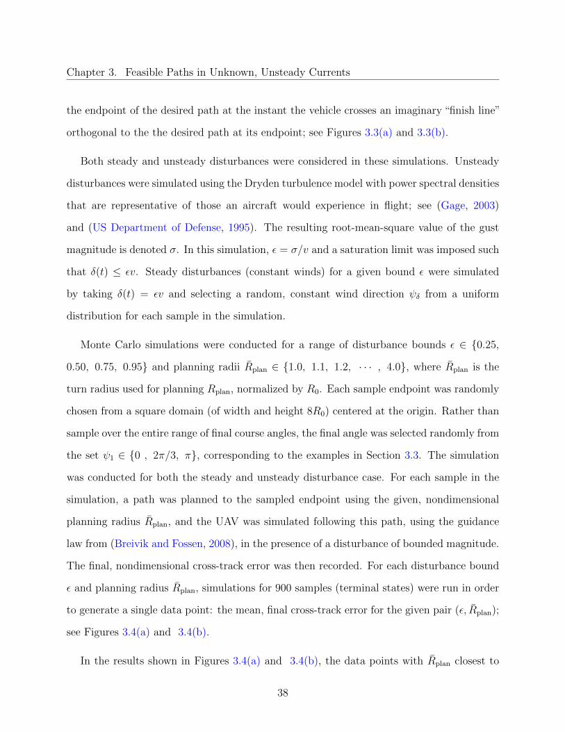
Chapter 3. Feasible Paths in Unknown, Unsteady Currents
the endpoint of the desired path at the instant the vehicle crosses an imaginary “finish line”
orthogonal to the the desired path at its endpoint; see Figures 3.3(a) and 3.3(b).
Both steady and unsteady disturbances were considered in these simulations. Unsteady
disturbances were simulated using the Dryden turbulence model with power spectral densities
that are representative of those an aircraft would experience in flight; see (Gage, 2003)
and (US Department of Defense, 1995). The resulting root-mean-square value of the gust
magnitude is denoted σ. In this simulation, ε = σ/v and a saturation limit was imposed such
that δ(t) ≤ εv. Steady disturbances (constant winds) for a given bound ε were simulated
by taking δ(t) = εv and selecting a random, constant wind direction ψδ from a uniform
distribution for each sample in the simulation.
Monte Carlo simulations were conducted for a range of disturbance bounds ε ∈ 0.25,
0.50, 0.75, 0.95 and planning radii Rplan ∈ 1.0, 1.1, 1.2, · · · , 4.0, where Rplan is the
turn radius used for planning Rplan, normalized by R0. Each sample endpoint was randomly
chosen from a square domain (of width and height 8R0) centered at the origin. Rather than
sample over the entire range of final course angles, the final angle was selected randomly from
the set ψ1 ∈ 0 , 2π/3, π, corresponding to the examples in Section 3.3. The simulation
was conducted for both the steady and unsteady disturbance case. For each sample in the
simulation, a path was planned to the sampled endpoint using the given, nondimensional
planning radius Rplan, and the UAV was simulated following this path, using the guidance
law from (Breivik and Fossen, 2008), in the presence of a disturbance of bounded magnitude.
The final, nondimensional cross-track error was then recorded. For each disturbance bound
ε and planning radius Rplan, simulations for 900 samples (terminal states) were run in order
to generate a single data point: the mean, final cross-track error for the given pair (ε, Rplan);
see Figures 3.4(a) and 3.4(b).
In the results shown in Figures 3.4(a) and 3.4(b), the data points with Rplan closest to
38

Chapter 3. Feasible Paths in Unknown, Unsteady Currents
1 2 3 40
0.1
0.2
0.3
0.4
0.5
0.6
Planning Radius
Me
an
Cro
ss T
rack E
rro
r
ε = 0.95
ε = 0.75
ε = 0.50
ε = 0.25
(a) Steady disturbance case
1 2 3 40
0.1
0.2
Planning Radius
Me
an
Cro
ss T
rack E
rro
r
ε = 0.95
ε = 0.75
ε = 0.50
ε = 0.25
(b) Unsteady disturbance case
Figure 3.4: Normalized mean, final cross-track error versus Rplan from Monte Carlo simula-tion
R′0/R0 = (1 + ε)2 for a given ε are emphasized with a solid marker. In both cases, the trend
is for the mean, final cross-track error to decrease as the planning radius increases until
a critical value of the planning radius is reached (the “knee” in the curve). At this critical
value, the mean, final cross-track error approaches a lower bound and no further performance
improvements are gained by using larger values of Rplan. This critical value of Rplan is of
interest because it indicates the smallest turn radius (and hence the shortest path) for which
the mean, final cross-track error is near its minimum value. For the steady disturbance case,
the paths planned using the feasible turn radius R′0 are very near the “knee” in the curve.
In the unsteady case, however, the the paths planned using R′0 are conservative; this result
is not surprising since the derivation of R′0 in Appendix A shows that the case of constant
disturbance magnitude and direction (δ = 0 and ψδ = 0) is the limiting case, requiring the
largest turn radius for feasibility.
39
Chapter 3. Feasible Paths in Unknown, Unsteady Currents
3.5 Conclusion
The ability to compensate for disturbances when following a Dubins path can be improved
by artificially increasing the turn radius used in path planning. Consider a Dubins car with
a nominal minimum turn radius R0 that is moving with a flow-relative speed v, subject to
unknown disturbances of bounded magnitude εv, with ε < 1. A Dubins path that is planned
using the turn radius R′0 = R0(1+ε)2 is feasible, in the sense that it could be exactly followed
if the disturbance were known. In practice, one typically uses feedback control to compensate
for an unknown disturbance. In this case, Monte Carlo simulations suggest that these feasible
Dubins paths (planned using the turn radius R′0) minimize the mean, final cross-track error
when the path is followed using a standard guidance algorithm. Furthermore, the simulation
results indicate that there is no appreciable benefit in planning paths with a turn radius
Rplan > R′0; the planning radius Rplan = R′0 marks the “knee” in the cross-track error curve
for a steady disturbance. Simulation results also suggest that choosing Rplan = R′0 may be
conservative for unsteady disturbances.
The cost of using the (sub-optimal) feasible turn radius R′0 for path planning is an increase
in the nominal path length and travel time. This tradeoff can be illustrated, for a given final
course angle, using a tradespace plot that indicates the relative path lengths of the optimal
(minimum length) and feasible Dubins paths. These tradespace plots can be helpful in
selecting a desired end state because they highlight regions where a given final state will
result in a large increase in the relative path length.
40

Chapter 4
Time-Optimal Path Planning with
Variable Speed Controls
4.1 Introduction
Gliders often operate at a glide slope that maximizes their forward speed. This glide slope
is steeper than the best lift-to-drag glide slope and reflects the priority of glider operators
to minimize transit time and overcome the effects of currents. Even at a legacy glider’s
top speed of about 20-30 cm/s, the effects of average ocean currents can challenge their
mobility. This problem is exacerbated in shallow water where the currents may be even
stronger; planning a minimum-time path becomes increasingly important. Minimum time
paths are also relevant whenever the glider is conducting a time sensitive mission or must
quickly change coarse to avoid a region with obstacles or other adverse conditions.
One limitation of Dubins path planning is that the path is planned assuming the vehicle
is operating at a fixed speed. However, most vehicles are capable of operating within an
41

Chapter 4. Time-Optimal Path Planning with Variable Speed Controls
interval of speeds. This interval typically ranges from a lower limit (a stall or idle speed) to
an upper limit (the maximum speed). Intuitively, one may think that a minimum-time path
implies always operating at the maximum speed. However, for a vehicle whose minimum
turn radius scales with speed, as occurs when the turn rate limits are fixed, one finds that
the minimum-time paths are not constructed solely from maximum-speed segments; time-
optimal paths are not simply Dubins paths. In this chapter, Dubins’ problem is revisited
while relaxing the constant speed constraint to allow an interval of strictly positive speeds.
To the author’s knowledge, the problem of constructing time-optimal paths for a kinematic
car with symmetric turn rate limits and whose forward speed varies within a strictly positive
interval has not been solved. Degtiariova-Kostova (2006) characterized the extremal controls
for a related problem, with turn acceleration and linear acceleration limits, however the path
synthesis problem was not solved. Perhaps the most relevant work is by Fedotov et al. (2011),
who considered a similar vehicle model and numerically constructed reachable sets in the
plane (representing position only) and in the three-dimensional configuration space (including
heading). There is an obvious connection between reachable sets and optimal paths; the time-
optimal solution corresponds to the case when the time-parameterized reachable set first
encounters the target state. Here the extremal controls are characterized directly, however,
and a finite and sufficient set of candidate optimal controls and a path synthesis procedure
are provided. The following work is adapted from (Wolek et al., 2015b).
42

Chapter 4. Time-Optimal Path Planning with Variable Speed Controls
4.2 Problem Formulation
Consider the modified Dubins-car model (2.10) where the speed is treated as a control input:
x(t) = v(t) cosψ(t) ,
y(t) = v(t) sinψ(t) ,
ψ(t) = u(t) .
The turn rate is symmetrically bounded: u ∈ [−umax, umax]. Choosing a modified distance
unit that gives a maximum speed of unity, v ∈ [vmin, 1] where vmin > 0 is the minimum speed.
Since v is strictly positive, the arc-length s along the path is monotonically increasing
and the independent variable may be transformed from t to s, recognizing that ds = v(s)dt.
Replacing the turn rate input u with κ = u/v, the system equations become
x′(s) = cosψ(s) , (4.1)
y′(s) = sinψ(s) , (4.2)
ψ′(s) = κ(s) , (4.3)
where the operator (·)′ denotes differentiation with respect to s. Without loss of generality,
take the initial set to be the single point x0 = (0 0 0)T and define the terminal set to
be the point x1 = (x1 y1 ψ1)T. A path from x0 to x1 begins with the initial arc-length
parameter s0 (which will generally be taken as zero) and ends with some (unknown) final
arc-length s1. Thus the initial conditions are given by
x(s0) = x0 . (4.4)
43
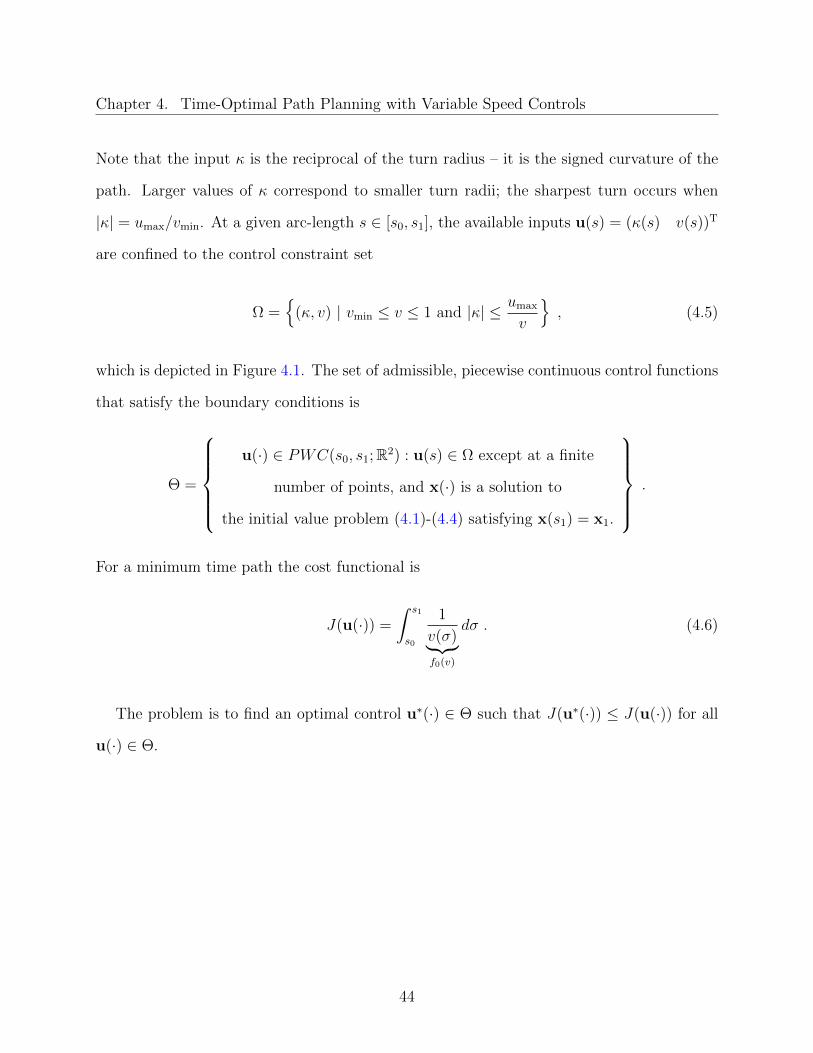
Chapter 4. Time-Optimal Path Planning with Variable Speed Controls
Note that the input κ is the reciprocal of the turn radius – it is the signed curvature of the
path. Larger values of κ correspond to smaller turn radii; the sharpest turn occurs when
|κ| = umax/vmin. At a given arc-length s ∈ [s0, s1], the available inputs u(s) = (κ(s) v(s))T
are confined to the control constraint set
Ω =
(κ, v) | vmin ≤ v ≤ 1 and |κ| ≤ umax
v
, (4.5)
which is depicted in Figure 4.1. The set of admissible, piecewise continuous control functions
that satisfy the boundary conditions is
Θ =
u(·) ∈ PWC(s0, s1;R2) : u(s) ∈ Ω except at a finite
number of points, and x(·) is a solution to
the initial value problem (4.1)-(4.4) satisfying x(s1) = x1.
.
For a minimum time path the cost functional is
J(u(·)) =
∫ s1
s0
1
v(σ)︸︷︷︸f0(v)
dσ . (4.6)
The problem is to find an optimal control u∗(·) ∈ Θ such that J(u∗(·)) ≤ J(u(·)) for all
u(·) ∈ Θ.
44

Chapter 4. Time-Optimal Path Planning with Variable Speed Controls
Figure 4.1: Control constraint set Ω
4.3 Applying the Minimum Principle
To apply the Minimum Principle, introduce the variational Hamiltonian
H(η0, ~η, x, y, ψ, κ, v) = η0f0(v) + 〈~η, ~f(ψ, κ)〉
= η0
(1
v
)+ ηx cosψ + ηy sinψ + ηψκ ,
where ~f(ψ, κ) = (fx fy fψ)T is the right hand side of the control system (4.1)-(4.3) and
~η = (ηx ηy ηψ)T is a vector of corresponding adjoint variables. (The explicit arc-length
dependence of the variables is suppressed for brevity.) The term f0(v) is the integrand of the
cost functional (4.6) and η0 is the associated adjoint variable. The Minimum Principle states
that if a control pair (κ∗, v∗) is optimal, then there exists a constant η0 ≥ 0 and absolutely
continuous functions ηx, ηy and ηψ such that
η′x = −∂H∂x
= 0 , (4.7)
η′y = −∂H∂y
= 0 , (4.8)
η′ψ = −∂H∂ψ
= ηx sinψ − ηy cosψ . (4.9)
45

Chapter 4. Time-Optimal Path Planning with Variable Speed Controls
(Note that a trivial solution to (4.7)-(4.9) is not admissible, and ηx and ηy remain constant
because the states x and y do not appear in the Hamiltonian.) Moreover,
min(κ,v)∈Ω
H(η∗0, ~η∗, x∗, y∗, ψ∗, κ, v) = H(η∗0, ~η
∗, x∗, y∗, ψ∗, κ∗, v∗) = 0 .
That is, the Hamiltonian is minimized with the optimal controls and equal to zero along the
optimal trajectory. Recalling that the adjoint variables ηx and ηy are constant, then
ηx = η cos θ, ηy = η sin θ , (4.10)
for some constants η and θ, so that the differential equation for ηψ can be rewritten as
η′ψ = η sin(ψ − θ) , (4.11)
and the variational Hamiltonian as
H(η0, η, ηψ, κ, v) = η0
(1
v
)+ ηψκ︸ ︷︷ ︸
Hc(η0,ηψ ,κ,v)
+η cos(θ − ψ) , (4.12)
where Hc(η0, ηψ, κ, v) is the control-dependent part of the Hamiltonian.
4.4 Geometric Approach - the Hodograph
Characterizing Extremal Controls
The control-dependent part Hc of the Hamiltonian (4.12) is given by
46
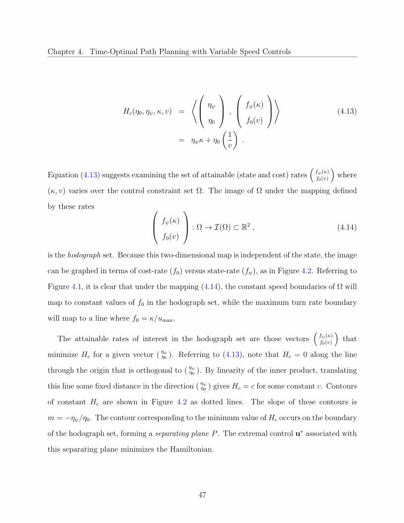
Chapter 4. Time-Optimal Path Planning with Variable Speed Controls
Hc(η0, ηψ, κ, v) =
⟨ ηψ
η0
,
fψ(κ)
f0(v)
⟩ (4.13)
= ηψκ+ η0
(1
v
).
Equation (4.13) suggests examining the set of attainable (state and cost) rates(fψ(κ)
f0(v)
)where
(κ, v) varies over the control constraint set Ω. The image of Ω under the mapping defined
by these rates fψ(κ)
f0(v)
: Ω→ I(Ω) ⊂ R2 , (4.14)
is the hodograph set. Because this two-dimensional map is independent of the state, the image
can be graphed in terms of cost-rate (f0) versus state-rate (fψ), as in Figure 4.2. Referring to
Figure 4.1, it is clear that under the mapping (4.14), the constant speed boundaries of Ω will
map to constant values of f0 in the hodograph set, while the maximum turn rate boundary
will map to a line where f0 = κ/umax.
The attainable rates of interest in the hodograph set are those vectors(fψ(κ)
f0(v)
)that
minimize Hc for a given vector ( ηψη0 ). Referring to (4.13), note that Hc = 0 along the line
through the origin that is orthogonal to ( ηψη0 ). By linearity of the inner product, translating
this line some fixed distance in the direction ( ηψη0 ) gives Hc = c for some constant c. Contours
of constant Hc are shown in Figure 4.2 as dotted lines. The slope of these contours is
m = −ηψ/η0. The contour corresponding to the minimum value ofHc occurs on the boundary
of the hodograph set, forming a separating plane P . The extremal control u∗ associated with
this separating plane minimizes the Hamiltonian.
47

Chapter 4. Time-Optimal Path Planning with Variable Speed Controls
Figure 4.2: The hodograph set, with subspaces of constant Hc drawn (dotted lines), for agiven adjoint vector
To identify the extremal controls for a particular adjoint vector, first consider the case
ηψ ≤ 0, as in the example shown in Figure 4.2. Following the Minimum Principle, it is clear
from the definition of Hc that with ηψ ≤ 0 the signed curvature should satisfy κ ≥ 0. For the
particular adjoint vector shown in Figure 4.2, the separating plane occurs at the corner where
the maximum turn rate and minimum speed constraints are active – the northeast corner
of the hodograph set. The separating plane is not unique there; infinitely many separating
planes pass through the corner, each corresponding to a unique adjoint vector.
The set of points (fψ, f0) along the maximum turn rate constraint, the eastern boundary
of the hodograph set, forms an angle φ with the vertical axis. Since this line is defined by
f0 = κ/umax, then tanφ = umax. Defining the angle χ = atan(
η0|ηψ |
), one may infer which
constraints are active for given values of ηψ. Assuming that η0 6= 0:
• If χ = π/2, then ηψ = 0, so that the vector ( ηψη0 ) points north and the separating
plane coincides with the maximum speed constraint – the southern boundary of the
hodograph set.
48

Chapter 4. Time-Optimal Path Planning with Variable Speed Controls
• If φ < χ < π/2, then η0|ηψ |
> umax and the separating plane passes through the maximum
speed and maximum turn rate constraints – the southeastern corner of the hodograph
set.
• If χ = φ, then η0|ηψ |
= umax and the separating plane coincides with the maximum turn
rate constraint – the eastern boundary of the hodograph set.
• If 0 ≤ χ < φ, then η0|ηψ |
< umax and the separating plane passes through the minimum
speed and maximum turn rate constraint – the northeastern corner of the hodograph
set.
If η0 = 0 and ηψ 6= 0, then χ is either 0 or π, so the minimizing input corresponds to
maximum turn rate and minimum speed. If η0 = 0 and ηψ = 0, then Hc = 0 regardless
of the choice of input and the min-H operation does not provide information regarding the
extremal controls. In this case, the extremal controls can be characterized by considering
the remaining necessary conditions of the Minimum Principle and by applying the Karush-
Kuhn-Tucker (KKT) conditions, as discussed in detail in Appendix B.1. The KKT conditions
indicate that when ηψ = 0, the optimal curvature is κ = 0. The analysis also reveals that
η0|ηψ |
= umax at only a finite number of isolated points; this situation need not be considered
in constructing candidate extremal paths.
In developing a synthesis method, note that extremal paths will comprise straight seg-
ments at maximum speed, “bang turns” at maximum speed and maximum turn rate, and
“cornering turns” at minimum speed and maximum turn rate. Denote these extremal fam-
ilies using the symbols S, B and C, respectively. The control conditions are annotated on
the control constraint set shown in Figure 4.1, for left turns, and they are summarized in
Table 4.1. The set of all extremal families is then F = S,B, C.
49

Chapter 4. Time-Optimal Path Planning with Variable Speed Controls
Symbol (Description) Condition ControlsS (Straight segment) ηψ = 0 v = 1
κ = 0(u = 0)
B (“Bang” turn) 0 < |ηψ| < η0umax
v = 1|κ| = umax
(|u| = umax)C (“Cornering” turn) |ηψ| > η0
umaxv = vmin
|κ| = umax/vmin
(|u| = umax)
Table 4.1: Summary of extremal families
Figure 4.3: Types of extremal paths
Parameterizing Extremal Paths
Having identified the extremal controls, it is useful to parametrize them by orientation and
length to aid in further analysis. Recall that the radius of a circular arc is the inverse of its
curvature. Thus, extremal paths corresponding to the B and C families are arcs with radius
R ≡ 1/umax and r ≡ vmin/umax, respectively. (Note that r < R, as shown in Figure 4.3.)
The extent of each segment can be indicated by a superscript corresponding to (i) the path
length L ≥ 0 for S segments or (ii) the subtended angle for circular arcs B or C. The
orientation of a turn can be denoted by the sign of the subtended angle (positive for left
turns, negative for right turns). For example, the sequence of controls CBSB, read left-to-
right, is uniquely defined by the parametrization Cα1Bα2SLBα3 . The cost of each extremal
50
Chapter 4. Time-Optimal Path Planning with Variable Speed Controls
control can be similarly parameterized. Since straight segments have v = 1, the change
in cost is numerically equal to the path length, ∆J = L/v = L. (Note however that the
dimension of the cost is time, not length. To avoid the confusion of seemingly inconsistent
dimensions, one may non-dimensionalize the problem parameters.) For both B and C turns,
the turn rate is always u = umax, so the change in cost is proportional to the angle subtended
by the turn (equivalently the change in heading |∆ψ|), so that ∆J = |∆ψ|/umax. Thus, for
example, the cost of the path Cα1Bα2SLBα3 is
∆J = L+1
umax
3∑i=1
|αi| .
4.5 Existence of An Optimal Control
The Dubins problem is a special case of the problem considered here where the speed is held
fixed. Since it has already been established that the Dubins problem is controllable (Dubins,
1957), it follows that the system considered here is also controllable. From Figure 4.2 it is
clear that the hodograph is convex. From the definition (5.6) it follows that Ω is a fixed,
nonempty, compact set. Then referring to Theorem 2.6.1 all of the conditions are satisfied
for the existence of an optimal control.
4.6 Properties of Extremal Controls
An extremal path is entirely determined by the behavior of the adjoint variable ηψ. The
extremal controls described in Table 4.1 can be written explicitly in terms of ηψ, for η0 6= 0,
51

Chapter 4. Time-Optimal Path Planning with Variable Speed Controls
as
(κ, v) =
(0, 1) if ηψ = 0
(−sgn(ηψ)/R, 1) if 0 < |ηψ| < η0/umax
(−sgn(ηψ)/r, vmin) if |ηψ| > η0/umax
. (4.15)
Thus ηψ can be thought of as a switching function that determines which extremal family
becomes active. (The cost-invariant case where η0 = 0, and the cost function does not appear
in the Hamiltonian, will be discussed later.) Changes in turn rate may occur where ηψ = 0,
whereas changes in speed may occur where |ηψ| = η0/umax. The extremal control equation
(4.15), the heading equation (4.3), and the adjoint equation (4.11) are closely coupled. A
careful study of this system of equations reveals which sequences of extremal controls are
admissible.
Extremal Controls With Fixed Turn Rate
Consider an extremal control for which the turn rate is fixed. This is equivalent to an adjoint
solution where ηψ does not change sign or vanish. Let the initial arc-length be s0, the initial
heading be ψ0, and the initial adjoint variable be ηψ(s0) = ηψ0 . Then from (4.11) and (4.3),
the adjoint history for a fixed κ is
ηψ(s) =η(cos(ψ0 − θ)− cos(κ(s− s0) + ψ0 − θ))
κ+ ηψ0 , (4.16)
where η and θ are defined in (4.10). Note the sinusoidal nature of the solution ηψ, and that
κ is fixed for a range of ηψ, given by (4.15). Since the curvature κ is larger for a C arc than
for a B arc, the amplitude and wavenumber of the sinusoid ηψ changes when ηψ crosses the
boundary where |ηψ| = η0/umax. In the region corresponding to a C arc, for example, the
amplitude is smaller and the wavenumber is higher. While the wavenumber and amplitude
52
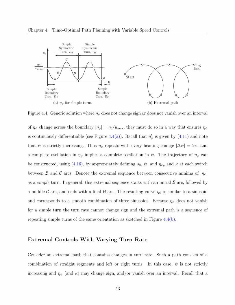
Chapter 4. Time-Optimal Path Planning with Variable Speed Controls
(a) ηψ for simple turns (b) Extremal path
Figure 4.4: Generic solution where ηψ does not change sign or does not vanish over an interval
of ηψ change across the boundary |ηψ| = η0/umax, they must do so in a way that ensures ηψ
is continuously differentiable (see Figure 4.4(a)). Recall that η′ψ is given by (4.11) and note
that ψ is strictly increasing. Thus ηψ repeats with every heading change |∆ψ| = 2π, and
a complete oscillation in ηψ implies a complete oscillation in ψ. The trajectory of ηψ can
be constructed, using (4.16), by appropriately defining s0, ψ0 and ηψ0 and κ at each switch
between B and C arcs. Denote the extremal sequence between consecutive minima of |ηψ|
as a simple turn. In general, this extremal sequence starts with an initial B arc, followed by
a middle C arc, and ends with a final B arc. The resulting curve ηψ is similar to a sinusoid
and corresponds to a smooth combination of three sinusoids. Because ηψ does not vanish
for a simple turn the turn rate cannot change sign and the extremal path is a sequence of
repeating simple turns of the same orientation as sketched in Figure 4.4(b).
Extremal Controls With Varying Turn Rate
Consider an extremal path that contains changes in turn rate. Such a path consists of a
combination of straight segments and left or right turns. In this case, ψ is not strictly
increasing and ηψ (and κ) may change sign, and/or vanish over an interval. Recall that a
53
Chapter 4. Time-Optimal Path Planning with Variable Speed Controls
change in turn rate requires ηψ = 0. (Thus ηψ = 0 will occur at the beginning and/or end
of a turn that connects to another extremal.) Any turn that contains such a point can be
classified as one of the following:
1. Flexible Turn. If η′ψ = 0 when ηψ = 0 (i.e., if ηψ intersects the s-axis tangentially),
call this a flexible turn. Because η′ψ must vary continuously, the value of η′ψ at a point
where ηψ = 0 determines what switches are admissible. If η′ψ = 0 when ηψ = 0, then
the control κ is not uniquely defined at this point; three values of κ are admissible. If
κ does not change sign, the trajectory continues on a B extremal arc of the original
sense. If κ = 0, then the heading does not change and η′ψ = 0, resulting in a switch
to a S extremal. Finally, if κ changes sign, then the heading rate changes sign; the
trajectory switches to a B extremal arc of the opposite sense. In this third case, it is
clear from (4.11) that the resulting segment of the curve ηψ will be antisymmetric to
the portion preceding it; see Figure 4.5(a).
2. Rigid Turn. If η′ψ 6= 0 when ηψ = 0 (i.e., if ηψ intersects the s-axis transversally,
as shown in Figure 4.6(a)), call this a rigid turn. In this case, the control κ must
change sign for the necessary conditions to be satisfied, and for ηψ to be continuously
differentiable. As was true for a flexible turn, the value of ηψ after crossing the s-axis
will be antisymmetric to the segment that precedes the crossing.
A Taxonomy for Extremal Turns
Each turn in an extremal sequence can be further classified as one of the following:
1. Symmetric Turn. Consider an extremal arc that begins with η(s2) = ηψ0 , and ends
with η(s3) = ηψ0 , but does not vanish on the open interval (s2, s3). On this interval, the
54

Chapter 4. Time-Optimal Path Planning with Variable Speed Controls
turn rate is fixed and the extremal path is a BCB sequence, as described in Section 4.6.
Since ηψ does not vanish on (s2, s3), then the closed interval [s2, s3] corresponds to (at
most) one complete oscillation in ηψ. It follows that ηψ is symmetric on [s2, s3] about
the vertical axis passing through (s2 + s3)/2. The initial and final B arcs in this BCB
sequence will be of equal length. Also, from symmetry η′ψ(s2) = −η′ψ(s3).
2. Boundary Turn. Consider a turn that begins and/or end at one of the two boundary
conditions defining the path optimization problem; such a turn is not required to both
begin and end with ηψ = ηψ0 .
With this taxonomy (see Figures 4.4(a), 4.5(a) and 4.6(a)), any extremal turn can be
classified as one of the following:
• simple: symmetric or boundary turn
• flexible: symmetric or boundary turn
• rigid: symmetric or boundary turn
Recall that flexible turns begin and/or end with η′ψ = 0 when ηψ = 0, and symmetric turns
begin and end with ηψ0 . Thus a flexible, symmetric turn has ηψ0 = 0 and corresponds to one
complete oscillation in ηψ. The change in heading during the turn is |∆ψ| = 2π.
Also, like a flexible, symmetric turn, a rigid, symmetric turn will be symmetric about the
midpoint between consecutive, isolated points where ηψ0 = 0. However, since the derivative
at these points satisfies η′ψ 6= 0, then they correspond to an incomplete oscillation in ηψ.
Thus the heading along a rigid, symmetric turn will satisfy |∆ψ| < 2π.
Boundary turns (flexible, rigid or simple) can be thought of as “fragments” of their cor-
responding symmetric (flexible, rigid or simple) turns that have been truncated to satisfy
given boundary conditions. The B arcs in the BCB extremal sequence of a boundary turn
55

Chapter 4. Time-Optimal Path Planning with Variable Speed Controls
(a) ηψ for flexible turns (b) Extremal path
Figure 4.5: Generic solution where ηψ intersects the s-axis tangentially
are not necessarily equal. However, it is clear that a B arc that does not join a boundary
condition, and instead connects to other extremals (where ηψ = 0), will be equal to or longer
than a B arc that does join a boundary condition.
These conditions are summarized in Table 4.2, after introducing some additional notation
describing the geometry of such turns.
Special Case: Dubins-like Paths
If η0 6= 0 and |ηψ| < umax/η0 on the interval [s0, s1], then the extremal path consists of only
B arcs and S segments. Since both of these extremals occur at the maximum speed v = 1,
the time optimal solution is also the minimum length solution – a Dubins path with arcs of
radius R, traversed at maximum speed. The solutions for this case are known to be of the
form BSB or BBB (Dubins, 1957).
If η0 = 0, the adjoint vector ( ηψη0 ) lies parallel to the abscissa of the hodograph. From
the discussion of the KKT conditions in Appendix B.1, only extremal sequences containing
56

Chapter 4. Time-Optimal Path Planning with Variable Speed Controls
(a) ηψ for rigid turns (b) Extremal path
Figure 4.6: Generic solution where ηψ intersects the s-axis transversally
C arcs (of radius r) and S segments are admissible. If an extremal sequence contains C arcs
and S segments, then along the S segments κ = 0, η′ψ = 0 and ηψ = 0. From (4.11) it follows
that for a nontrivial solution to the adjoint equation η 6= 0 is required, and thus the heading
must be ψ = θ + kπ where k ∈ Z. But from (4.12), a necessary condition for optimality is
H = η cos(ψ− θ) = 0, which cannot be satisfied with ψ = θ+ kπ. Thus, S segments are not
admissible. Only C arcs need to be considered. For such arcs the speed is fixed, v = vmin.
For a fixed speed, Dubins’ result then implies that the minimum length path is also the
minimum time path, and is of the form CSC or CCC. However, S arcs are not admissible.
Thus it can only be of the form CCC. The extremal control is then given by
(κ, v) = (−sgn(ηψ)1/r, vmin) , (4.17)
where ηψ = 0 can only occur at isolated points.
57

Chapter 4. Time-Optimal Path Planning with Variable Speed Controls
Geometry of Extremal Turns
A generic extremal turn with ηψ crossing the |ηψ| = η0/umax boundary is of the form BCB.
To parameterize such turns, let the first B arc subtend an angle α, the C arc subtend an angle
β, and the final B arc subtend an angle γ (where all the segments are of the same orientation,
and the sign of the angle denotes a left or right turn). Denote this turn as BαCβBγ. The
change in heading is ∆ψ = α + β + γ. Given an initial heading angle ψ0, the displacements
in the plane resulting from this turn are:
∆x =R(sin(α + β + γ + ψ0)− sin(ψ0)) + (R− r)(sin(α + ψ0)− sin(ψ0 + α + β)) , (4.18)
∆y =R(cos(ψ0)− cos(α + β + γ + ψ0)) + (R− r)(cos(α + β + ψ0)− cos(α + ψ0)) . (4.19)
This is a general representation of any BCB turn. Note, however, that it is possible for
certain segments to have zero length. If the turn is a symmetric turn then α = γ. Otherwise
it must begin and/or end at a boundary condition and in general α 6= γ. Since both B and C
extremals correspond to arcs with the same maximum turn rate, the cost is proportional to
the heading change along each arc, even though they are traversed at different speeds. For
a generic BαCβBγ turn the change in cost is ∆J = R|∆ψ| = R(|α|+ |β|+ |γ|).
Admissible Extremal Control Sequences
For brevity, let T (α, β, γ) denote the generic turn BαCβBγ. If |ηψ| does not vanish, the turn
is a simple turn. If |ηψ| does vanish, then depending on the value of η′ψ at the point where
ηψ = 0, the turn is either a flexible turn or a rigid turn. Furthermore, if the turn occurs in
the middle of an extremal control sequence it must be a symmetric turn. If the turn occurs
at a boundary condition (B.C.), then it is not necessarily symmetric and is called a boundary
58
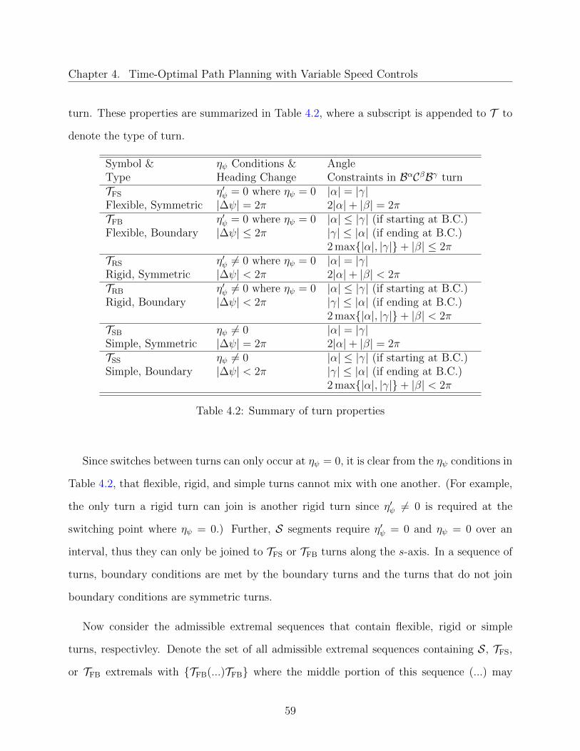
Chapter 4. Time-Optimal Path Planning with Variable Speed Controls
turn. These properties are summarized in Table 4.2, where a subscript is appended to T to
denote the type of turn.
Symbol &Type
ηψ Conditions &Heading Change
AngleConstraints in BαCβBγ turn
TFS
Flexible, Symmetricη′ψ = 0 where ηψ = 0|∆ψ| = 2π
|α| = |γ|2|α|+ |β| = 2π
TFB
Flexible, Boundaryη′ψ = 0 where ηψ = 0|∆ψ| ≤ 2π
|α| ≤ |γ| (if starting at B.C.)|γ| ≤ |α| (if ending at B.C.)2 max|α|, |γ|+ |β| ≤ 2π
TRS
Rigid, Symmetricη′ψ 6= 0 where ηψ = 0|∆ψ| < 2π
|α| = |γ|2|α|+ |β| < 2π
TRB
Rigid, Boundaryη′ψ 6= 0 where ηψ = 0|∆ψ| < 2π
|α| ≤ |γ| (if starting at B.C.)|γ| ≤ |α| (if ending at B.C.)2 max|α|, |γ|+ |β| < 2π
TSB
Simple, Symmetricηψ 6= 0|∆ψ| = 2π
|α| = |γ|2|α|+ |β| = 2π
TSS
Simple, Boundaryηψ 6= 0|∆ψ| < 2π
|α| ≤ |γ| (if starting at B.C.)|γ| ≤ |α| (if ending at B.C.)2 max|α|, |γ|+ |β| < 2π
Table 4.2: Summary of turn properties
Since switches between turns can only occur at ηψ = 0, it is clear from the ηψ conditions in
Table 4.2, that flexible, rigid, and simple turns cannot mix with one another. (For example,
the only turn a rigid turn can join is another rigid turn since η′ψ 6= 0 is required at the
switching point where ηψ = 0.) Further, S segments require η′ψ = 0 and ηψ = 0 over an
interval, thus they can only be joined to TFS or TFB turns along the s-axis. In a sequence of
turns, boundary conditions are met by the boundary turns and the turns that do not join
boundary conditions are symmetric turns.
Now consider the admissible extremal sequences that contain flexible, rigid or simple
turns, respectivley. Denote the set of all admissible extremal sequences containing S, TFS,
or TFB extremals with TFB(...)TFB where the middle portion of this sequence (...) may
59

Chapter 4. Time-Optimal Path Planning with Variable Speed Controls
contain any combination of TFS and S segments. Denote the set of all admissible extremal
sequences containing TRS or TRB turns with TRB(...)TRB where the middle portion of this
sequence (...) can contain any combination of TRS turns (with consecutive turns being of the
opposite sense). Last, denote the set of all admissible extremal sequences containing TSB or
TSS extremals with TSB(...)TSB where the middle portion of this sequence (...) can contain
any number of TSS turns (with consecutive turns being of the same sense).
If the turns are not of the generic form BCB then the extremals can belong to the Dubins-
like set: ΓDubins = BSB,BBB, CCC.
4.7 Additional Optimality Conditions
The geometry of the problem can be exploited to identify sub-optimality conditions that re-
duce the admissible extremal control sequences TFB(...)TFB, TRB(...)TRB and TSB(...)TSB
into a finite set of candidate optimal controls. Several such sub-optimality conditions are
derived in Appendices B.2, B.3 and B.4, and are discussed in the following.
In Appendix B.2 it is shown that a symmetric turn BαCβBγ is sub-optimal if the B arcs,
subtending angles γ = α, are sufficiently large (as shown in Figure B.1). This sub-optimality
condition occurs when |α| ≥ |αsubopt| with αsubopt given by (B.12). Furthermore, it is shown
that a flexible, symmetric turn with |∆ψ| = 2π always violates this condition and therefore
is sub-optimal in general. This implies that the middle portion (...) of the set TFB(...)TFB
contains only straight segments (or rather one straight segment) so that the largest element
in TFB(...)TFB, in terms of the number of extremal switches, can be parametrized as
TFBSTFB = Bα1Cβ1Bγ1SLBα2Cβ2Bγ2 .
60

Chapter 4. Time-Optimal Path Planning with Variable Speed Controls
In Appendix B.3, optimality conditions are derived for the turning portion of a ST FB or
TFBS segment. It is shown that for the ith turn in TFBSTFB (where i = 1 or 2):
if |βi| < π, then γi = 0 for ST FB segments
or αi = 0 for TFBS segments
else |βi| = π .
Also, from previous considerations:
|αi|+ |βi|+ |γi| < 2π , (4.20)
sgn(αi) = sgn(βi) = sgn(γi) , (4.21)
min|αi|, |γi| < αsubopt , (4.22)
and
|αi| ≤ |γi| for ST FB segments , (4.23)
|γi| ≤ |αi| for TFBS segments .
Note that the seven parameters defining TFBSTFB = Bα1Cβ1Bγ1SLBα2Cβ2Bγ2 cannot vary
independently; they must satisfy the necessary conditions above. Any extremal of this type
is uniquely described by (at most) four parameters, and is an element of the set:
ΓT ST = BCBSBCB,BCBSBC,BCBSB, CBSBCB, CBSBC, CBSB,BSBCB,BSBC .
While it is possible for two elements in ΓT ST to describe the same extremal sequence (for
example, if one of the parameters is zero), in general each of these elements corresponds
61

Chapter 4. Time-Optimal Path Planning with Variable Speed Controls
to a unique type of candidate path to consider. Furthermore, each element of ΓT ST may
have four possible orientations (LSL, LSR, RSL, RSR, as in Dubins path planning, see
Section 2.7) that need to be considered.
In Appendix B.4 it is shown that the extremal sequence BTRSB (with equal length B arcs)
is sub-optimal. The largest element in the set TRB(...)TRB that does not contain this sub-
optimal sequence is BTRSTRSB, which can be parameterized as Bγ1(Bα2Cβ2Bγ2)(Bα3Cβ3Bγ3)Bα4 .
The parentheses in this expression are used to emphasize that consecutive turns are of the
opposite sense; recall that a BCB sequence is a single turn. For any sequence of three
consecutive turns i, j, and k
min|γi|, |αk| < |αj| , (4.24)
is required for the sequence to not contain a sub-optimal BTRSB segment with equal B
arcs. Additional necessary conditions are that two consecutive turns i and j are always of
the opposite sense so that sgn(γi) = −sgn(αj), and unless one of them joins a boundary
condition |γi| = |αj| and |βi| = |βj|. With these conditions, the set TRB(...)TRB reduces to
the finite set of at most four turns:
ΓT T T T = BT T B,BT BCB,BT BC,BT B,BBCB,BCBT B,
BCBBCB,BCBBC,BCBB, CBT B, CBBCB, CBBC
where, as previously, each element of this set is described by (at most) four parameters. Note
that each element in this set can either begin with a left or right turn. Thus there are two
orientations to consider for each candidate.
Last, it remains to consider the simple turn candidates discussed in Section 4.6, for which
the turn rate is fixed |u| = umax. In this case, the admissible controls are contained in the
set TSB(...)TSB. Recall that TSS turns have a heading change |∆ψ| = 2π. However, in
62
Chapter 4. Time-Optimal Path Planning with Variable Speed Controls
Appendix B.2 it is shown that any symmetric turn subtending 2π is sub-optimal. Thus TSS
turns are sub-optimal in general, and TSB(...)TSB reduces to the set TSBTSB = BCBBCB
(with the condition that the initial and final B arcs are truncated so that neither TSB turn
subtends 2π.) Now, consider extremal sequences that are subsets of BCBBCB. The sequences
in the set BBCB,BCBB,BCB,BC, CB satisfy the same constraints as the BBCB sequence
in ΓT T T T and are not unique. Thus they can be ignored. Therefore, for a fixed turn rate,
the remaining unique admissible extremals are in the set
Γumax = BCBBCB, BCBBC, CBBCB, CBBC , (4.25)
where, as previously, each element of this set is described by (at most) four parameters, and
two orientations. While certain elements of ΓT ST and ΓT T T T may appear similar to those
of Γumax , the parameter constraints in each case are unique.
Having reduced the admissible extremal sequences from Section 4.6 to a finite number,
it follows that the optimal control is contained in the finite and sufficient set of candidate
optimal controls:
Γ = ΓT T T T ∪ ΓT ST ∪ Γumax ∪ ΓDubins . (4.26)
Since there are 12 members in the family ΓT T T T with two possible orientations, 8 members
in ΓT ST with four possible orientations, 4 members in Γumax with two possible orientations,
and 8 Dubins-like candidates, then Γ contains 72 unique types of candidate optimal controls.
4.8 Path Synthesis
The candidate optimal paths in ΓT T T T ∪ ΓT ST ∪ Γumax are defined by a finite-dimensional
parameter vector and three boundary conditions. Recall that the set ΓDubins is already fully
63

Chapter 4. Time-Optimal Path Planning with Variable Speed Controls
characterized as discussed in Section 2.7. Since the boundary conditions are nonlinear, and
the problem is under-determined, the solutions are difficult to characterize. Note that while
a finite set of candidate optimal controls has been defined and each element of this set can be
parametrized by a finite number of parameters, the parameter space itself is infinite and there
may be many solutions to the problem. One might seek to derive further optimality condi-
tions to obtain additional parameter constraints, however this can be laborious and there is
no guarantee of success. The approach taken in this work is to formulate a series of numerical
optimization problems to find local optima for each candidate in ΓT T T T ∪ ΓT ST ∪ Γumax
from which the lowest-cost solution can be chosen. A numerical optimization routine that
enumerates all locally optimal solutions would always give the globally optimal control (ac-
curate to within a user specified tolerance). In practice however, it is difficult to construct
such an algorithm. One may therefore expect only locally optimal paths, in general.
A Finite Dimensional Optimization Problem
A total of 64 candidate paths have been identified in ΓT T T T ∪ ΓT ST ∪ Γumax (accounting for
all the possible orientations of each turn), where each path is defined by a finite-dimensional
parameter vector p (in most cases p ∈ R4). For each candidate, the associated constrained
optimization problem is of the form:
min J(p) = cTp+ k , (4.27)
subject to Ap ≤ b ,
g(p) = 0 ,
h(p) ≤ 0 .
64
Chapter 4. Time-Optimal Path Planning with Variable Speed Controls
Assuming without loss of generality that x0 = (0 0 0)T and given a final endpoint x1 =
(x1 y1 ψ1)T, and the turn radii R and r, a numerical solver may return a locally optimal
solution to the problem (4.27), if one exists. The cost J(p) is a linear function of the
parameters since the cost is proportional to the durations of each path segment given by
p. The linear inequality constraints of the form Ap ≤ b, arise from the constraints on the
relative magnitudes of the angles and lengths that define each candidate path. The boundary
conditions are nonlinear equality constraints:
g(p) =
x(p)− x1
y(p)− y1
ψ(p)− ψ1
= 0 ,
where xp = (x(p) y(p) ψ(p))T is the terminal state for a given parameter vector p. The
inequality constraints h(p) ≤ 0 come from the strict inequality (4.22). (To enforce the
strict inequality using a non-strict inequality required by a numerical solver, solutions that
converge with h(p) = 0 are discarded since they are sub-optimal.) To select a suitable initial
guess that is close to a feasible candidate, a total of n guesses are uniformly sampled from
the closed, convex, polytope defined by Ap ≤ b. Each guess is then compared to the desired
endpoint x1 using the normalized error ε(p) :
ε(p) =
√(x(p)− x1)2 + (y(p)− y1)2√
x21 + y2
1
+|ψ(p)− ψ1|
2π.
The sample with the lowest normalized error is referred to as p0 and is used as an initial
guess, to solve the root finding problem g(p) = 0 that satisfies the boundary conditions. The
resulting root p′0 may not necessarily satisfy the constraint Ap′0 ≤ b anymore, however it is
assumed that this solution is within a sufficiently small neighborhood of the local optimum
for convergence. Then (4.27) is solved using the MATLAB (2013) constrained optimization
65

Chapter 4. Time-Optimal Path Planning with Variable Speed Controls
routine fmincon, with the initial guess p′0 to give p∗. The procedure is repeated for all
candidates in ΓT T T T ∪ ΓT ST ∪ Γumax . For every candidate that converges the path type,
parameter vector p∗ and cost are recorded.
Last, the remaining eight candidate paths in the set ΓDubins are computed using a standard
Dubins path planner with radius R or r, as appropriate. Having computed all candidate
optimal controls, it remains to compare their respective costs and identify the lowest cost
(locally optimal) solution.
4.9 Illustrative Examples
Let R = 1 and r = 0.3, and consider the desired terminal state x1 = (0 2 2π/3)T. The
results of the algorithm described in Section 4.8 for this endpoint are shown in Table 4.3,
and the associated paths are illustrated in Figures 4.7 and 4.8. In these figures, solid circles
denote boundary conditions and open circles denote switching points, where the type of path
segment changes. The lowest cost solution is of the form CBSB with orientation LSR, as
evident by comparing costs in Table 4.3. Note that the solutions beginning with a left turn
are generally lower cost that those beginning with a right turn. The terminal state is too far
away for a CCC Dubins-like solution to exist, but is close enough for BSB and BBB solutions;
however, these require significant maneuvering (see Figure 4.8) and have a high cost. A naive
planning approach using just the Dubins planner at maximum speed (with arcs of radius R)
would result in a path that takes about twice as long to traverse as the lowest cost solution
identified here. With this approach, only 13 of 72 candidate paths converged to a locally
optimal solution. It is possible that other locally optimal solutions exist. Since these cannot
be compared with the 13 candidate paths, global optimality cannot be claimed.
Having considered a particular case in detail, several additional paths are computed for a
66

Chapter 4. Time-Optimal Path Planning with Variable Speed Controls
Family ExtremalSequence
Orientation Cost
ΓT ST BCBSBCB RSR 11.278ΓT ST BCBSB RSL 6.615ΓT ST CBSBCB RSR 11.359ΓT ST CBSBC LSL 3.176ΓT ST CBSB LSL 2.883ΓT ST CBSB LSR 2.875ΓT T T T BCBB LR 2.887ΓT T T T BT B RLR 3.219Γumax CBBCB LL 8.378ΓDubins BBB RLR 5.980ΓDubins BSB LSR 9.378ΓDubins BBB RSL 8.015ΓDubins BSB RSR 14.078
Table 4.3: Locally optimal solutions, and associated costs, for the terminal state x1 =(0 2 2π/3)T
−2 −1 0 1 2 3−2
−1
0
1
2
3
x
Figure 4.7: Locally optimal paths from the set ΓT T T T ∪ ΓT ST ∪ Γumax for the terminalstate x1 = (0 2 2π/3)T
67

Chapter 4. Time-Optimal Path Planning with Variable Speed Controls
2 1 0 1 2 32
1
0
1
2
3
x
y
Figure 4.8: Locally optimal paths from ΓDubins for the terminal state x1 = (0 2 2π/3)T
grid of endpoints around the origin. In Figures 4.9, 4.10 and 4.11 the endpoints are plotted
for a particular “partition” of the plane for which the required final heading is held fixed
at ψ1 = 0, 2π/3 and π, respectively. In some cases the optimal path is a Dubins solution
(consider the endpoints x1 = (2 2 0)T or x1 = (2 − 2 0)T as shown in Figure 4.9),
however the majority of the paths involve cornering turns. There may also be multiple
optimal solutions. For example, reflecting the path for x1 = (−2 0 π)T (see Figure 4.11)
in the x-axis gives an equal cost path to the endpoint by symmetry.
4.10 Conclusion
The minimum-time path planning problem for a kinematic car with variable (strictly positive)
speed and symmetric turn rate limits was investigated. The kinematic car was used to model
the planar motion of an underwater glider with a speed that varies from the stall speed to the
maximum forward speed. The extremal controls were found to consist of: maximum turn rate
68

Chapter 4. Time-Optimal Path Planning with Variable Speed Controls
3 2 1 0 1 2 33
2
1
0
1
2
3
y
x
Figure 4.9: Lowest-cost paths for a grid of terminal states with ψ1 = 0
3 2 1 0 1 2 33
2
1
0
1
2
3
y
x
Figure 4.10: Lowest-cost paths for a grid of terminal states with ψ1 = 2π/3
69

Chapter 4. Time-Optimal Path Planning with Variable Speed Controls
2 1 0 1 23
2
1
0
1
2
3
y
x
Figure 4.11: Lowest-cost paths for a grid of terminal states with ψ1 = π
and maximum speed turns (denoted as B extremals), straight segments at maximum speed (S
extremals), and cornering turns (C extremals) with maximum turn rate and minimum speed.
An extremal turn was found, in general, to be a sequence of three consecutive extremals of
the form BCB. A finite and sufficient set of candidate optimal controls Γ was derived by
analysis of the adjoint differential equations, and by identifying sub-optimality conditions
geometrically. Candidate paths in Γ were found to consist of (at most) a sequence of four
turns, or a turn-straight-turn sequence. A numerical approach to solve for each candidate
path was proposed, so that the lowest cost solution could be identified. In some cases, the
resulting paths were substantially faster paths when compared to the (maximum speed)
Dubins path planning approach.
70
Chapter 5
Energy-Optimal Path Planning with a
Quadratic Glide Polar
5.1 Introduction
Underwater gliders are buoyancy driven vehicles that convert potential energy into forward
flight. To improve efficiency a natural objective is to plan paths that minimize the change
in depth for a given range (equivalently, maximize range for a given change in depth). This
is particularly important in shallow waters where the glider is forced to perform energy-
intensive buoyancy changes more frequently that can reduce the endurance of the glider. In
gliding flight, there is a tradeoff between the minimum turning radius and the depth rate
since both depend on the speed of the glider. (At slower speeds the glider can turn more
sharply, but with an increased depth rate.) Here a path planning problem that approximately
captures this tradeoff is investigated. As before, a modified Dubins car motion model (2.10)
is assumed (an interval of strictly positive speeds are admissible) and a cost functional that
minimizes the change in depth is considered. The relationship between the depth rate (or
71

Chapter 5. Energy-Optimal Path Planning with a Quadratic Glide Polar
“sink rate” in the sailplane community) and speed is often called the “glide polar”. Here the
glide polar is assumed to be a quadratic function of the speed recognizing that this restricts
the results to small bank angles and shallow turns. (See Section 5.2 for a discussion of this
assumption.)
The flight mechanics of underwater gliders and sailplanes are closely related. However,
one major difference is that buoyancy, in the case of underwater gliders, typically reduces
the required lift force required for vertical equilibrium. The small “net weight” (difference
between buoyancy and dry weight) explains, in part, the relatively slow speeds of underwater
gliders. While sailplanes typically seek sources of lift (such as thermals, ridge lift, lee waves,
etc.) to gain altitude, underwater gliders are able to actively adjust their buoyancy to return
to the surface. In the following some relevant work related to unpowered flight in still air (in
the absence of lift sources) is discussed.
An area of relevant work concerns emergency landing paths for powered aircraft experi-
encing a loss of thrust. At a low altitude after experiencing a loss of thrust during climb-out,
the Federal Aviation Administration (1987) recommends selecting a landing site within a
60 degree heading angle downrange from the point of failure. Alternately, one faces the
so called “impossible turn” problem studied by Rogers (1995) where the task is to maneu-
ver with minimum altitude loss and return to the end of the runway safely (with any final
heading angle). Ignoring transient motions, it has been shown that the steady-state optimal
path, in this case, is tear-drop shaped, consisting of a 45-degree bank angle turn at the stall
speed followed by a best glide slope straight segment (Rogers, 1995). Related studies have
considered the problem of maximizing range in a given direction (that is parallel, but not
necessarily coincident, with the runway) (Hoffren and Raivio, 2000), or to the nearest point
along the runway (Brinkman and Visser, 2007). However, in all of these studies, the final
endpoint is not fully constrained and hence the boundary conditions differ from the problem
72

Chapter 5. Energy-Optimal Path Planning with a Quadratic Glide Polar
considered here (where both the final planar position and final heading are specified).
If an aircraft experiences loss of thrust at a high enough altitude then it may be able to
perform a wider range of turning motions safely. There may be several suitable landing sites
to consider. (The search need not be restricted to areas directly downrange, as previously
discussed.) The emergency landing problem then requires planning a path to each candidate
landing site and comparing the associated altitude loss with each path. This case is perhaps
the most relevant to the present work, since the boundary conditions and the objective are
the same – to glide to a desired point with a specified final heading angle while minimiz-
ing altitude loss. Graph-based approaches are particularly useful to determine the landing
trajectory when obstacles are present (Adler et al., 2012). In the absence of obstacles, the
Dubins path planning approach has been proposed to quickly compare several landing sites
(Atkins et al., 2006; Eng et al., 2010).
Another related problem concerns the deployment of a glider to a desired point, with a
free heading angle, while maximizing endurance (Walton E. Williamson Jr., 1979; Chern,
1984). This problem was considered in the context of a military aircraft deploying a gliding
weapon, wherein the goal was to maximize the time to impact the target so that the aircraft
can escape to safety. In this case, however, the cost function differs from the problem
considered here.
The following work is adapted from (Wolek and Woolsey, 2015b).
5.2 The Glide Polar
The sink rate is often expressed as a function of the glider’s speed using the glide polar
sketched in Figure 5.1. The glide polar illustrates the relationship between horizontal speed
73

Chapter 5. Energy-Optimal Path Planning with a Quadratic Glide Polar
Figure 5.1: A typical glide polar
v and sink rate w for a glider in steady flight. (Typically v is the flow-relative speed,
however in the absence of a flow-field this is equivalent to ground speed.) The angle between
the horizontal axis and the ray emanating from the origin to a point (v, w) along the curve
gives the corresponding flight path angle γ. Several important flight conditions are labeled
on the glide polar in Figure 5.1: the “stall speed” vstall, the “minimum sink” speed vms, the
“speed to fly” vstf and the maximum speed vmax.
Flying in a straight line at the minimum sink speed vms gives the lowest sink rate and will
minimize the loss of altitude per unit time; this speed will maximize endurance. However,
an observation well known to sailplane pilots (MacCready, 1954) is that flying faster, at the
speed to fly vstf (also called the “best glide speed”), maximizes range per unit altitude and
minimizes the magnitude of the flight path angle γ. The following assumptions are made
about the glide polar:
Assumption 5.2.1. The glider polar is given by w(v) = av2 + bv + c, where a > 0, v ∈
[vstall, vmax] and w(v) > 0.
Similar assumptions of a quadratic glide polar are often made in the literature (Finke,
1992). The range of w(v) excludes the possibility of a zero sink rate (as might occur in
an updraft for example), and the assumption that a > 0 implies that w(v) is convex. It is
74
Chapter 5. Energy-Optimal Path Planning with a Quadratic Glide Polar
assumed that the stall speed vstall > 0.
Assumption 5.2.2. The minimum sink speed occurs at the critical point vms ∈ (vstall, vmax).
The critical point of w(v) occurs at vms = −b/2a so that w(vms) = −b2/4a + c. Since
vms > 0 and w(v) > 0 is required, it follows that b < 0 and c > b2/(4a).
Assumption 5.2.3. The speed to fly occurs at vstf ∈ (vstall, vmax).
The speed to fly is the point along the glide polar where the tangent line to the polar passes
through the origin (MacCready, 1954; Danewid, 1988) as shown in Figure 5.1; equivalently,
it is the speed at which ddvw(v) = w(v)/v. Given the previous assumptions, this condition is
satisfied at vstf =√c/a with vstf > vms.
Assumption 5.2.4. The minimum sink speed occurs at least half way between the stall speed
and the speed to fly: vms > (vstall + vstf)/2
This condition is a simplifying assumption used in the derivation of the extremal controls.
It is shown in Section 5.9 that this is a reasonable assumption in the example case considered,
however not all glide polars will satisfy this condition. The shape of the glide polar (and
hence the stall speed, minimum sink speed, and speed to fly) is largely determined by the
drag characteristics of an aircraft and thus this holds for a particular configuration (e.g. flap
setting).
Remark 5.2.1. Typically, there is no experimental data for gliders in turning flight. How-
ever, it is possible to estimate the sink rate in a turn from level flight polar data as discussed
in (Milgram, 2005). Alternatively, an energy-turn analysis provides a link between load-
factor, turn-rate and energy-rate; see (Cliff et al., 1982, 1992; Halter and Cliff, 1991) for
related discussions. This energy-turn approach may be used to derive the sink rate as a func-
tion of both the turn rate (or the load factor) and speed w(u, v) as shown in Chapter 6. In
75

Chapter 5. Energy-Optimal Path Planning with a Quadratic Glide Polar
this Chapter, however, it is assumed that the sink rate w(v) is independent of the turn rate
u, recognizing that this only holds for small bank angles and shallow turns.
5.3 Problem Formulation
Consider the projected planar motion of a glider (as viewed from above) where (x, y) ∈ R2
is the planar position of the vehicle and ψ ∈ [0, 2π) is its heading. The equations of motion
for this model with speed v and turn rate u controls are:
x(t) = v(t) cosψ(t) , (5.1)
y(t) = v(t) sinψ(t) , (5.2)
ψ(t) = u(t) . (5.3)
The turn rate control is symmetrically bounded u ∈ [−umax, umax]. The speed control in-
terval is strictly positive v ∈ [vstall, vmax] with vstall > 0. The control input function is then
u(·) = (u(·) v(·))T. Assuming quasi-steady flight, the cost functional J(u(·)) is defined as
the integral of the sink rate w(v) in wings-level (i.e. non-turning) flight, that satisfies the
assumptions in Section 5.2. Thus the total altitude loss is:
J(u(·)) =
∫ t1
t0
(av(τ)2 + bv(τ) + c
)dτ . (5.4)
Let the boundary conditions include the initial state x0 = (0 0 0)T and an initial time t0,
and the terminal state x1 = (x1 y1 ψ1)T and some unknown final time t1 > t0. Thus the
initial conditions are given by
x(t0) = x0 . (5.5)
76
Chapter 5. Energy-Optimal Path Planning with a Quadratic Glide Polar
Define the control constraint set
Ω = (u, v) | vstall ≤ v ≤ vmax and |u| ≤ umax . (5.6)
Then the set of piecewise continuous admissible controls that satisfy the boundary conditions
is
Θ =
u(·) ∈ PWC(t0, t1;R2) : u(s) ∈ Ω except at a finite
number of points, and x(·) is a solution to
the initial value problem (5.1)-(5.5) satisfying x(t1) = x1.
.
The problem is to find an optimal control u∗(·) ∈ Θ such that J(u∗(·)) ≤ J(u(·)) for all
u(·) ∈ Θ.
5.4 Existence of an Optimal Control
The Dubins problem satisfies the same state equations (5.1)-(5.3) as the problem considered
here, but with the available speed interval restricted to a single point (a fixed speed is
assumed). Since it has already been established that the Dubins car is controllable (Dubins,
1957), it follows that the system considered here is also controllable.
An optimal control exists for a system in the form x = ~f(x,u) with a Hamiltonian that is
strictly convex in the controls assuming ~f(x,u) satisfies certain continuity and boundedness
assumptions, as stated in (Steinberg and Stalford, 1973). One can easily verify that these
conditions in are satisfied by the system considered here, therefore an optimal control exists.
77
Chapter 5. Energy-Optimal Path Planning with a Quadratic Glide Polar
5.5 Applying the Minimum Principle
To apply the Minimum Principle, the variational Hamiltonian is introduced
H = η0w(v) + 〈~η, ~f(ψ, u, v)〉
= η0
(av2 + bv + c
)+ v(ηx cosψ + ηy sinψ) + ηψu ,
where ~f(ψ, u, v) is the right hand side of the state-system (5.1)-(5.3) and ~η = (ηx ηy ηψ)T is
a vector of corresponding adjoint variables. (The explicit time dependence of the variables is
suppressed for brevity.) Also, w(v) is the integrand of the cost-functional (5.4) and η0 is the
associated adjoint variable. The Minimum Principle states that if a control pair (u∗, v∗) is
optimal, then there exists a constant η0 ≥ 0 and absolutely continuous functions ηx(·), ηy(·)
and ηψ(·) such that
ηx(t) = −∂H∂x
= 0 , (5.7)
ηy(t) = −∂H∂y
= 0 , (5.8)
ηψ(t) = −∂H∂ψ
= v(t)(ηx sinψ(t)− ηy cosψ(t)) . (5.9)
(Note that a trivial solution to (5.7)-(5.9) is not admissible, and ηx and ηy remain constant
because the states x and y do not appear in the Hamiltonian.) Moreover,
min(u,v)∈Ω
H(η∗0, ~η∗, x∗, y∗, ψ∗, u, v) = H(η∗0, ~η
∗, x∗, y∗, ψ∗, u∗, v∗) = 0 .
78

Chapter 5. Energy-Optimal Path Planning with a Quadratic Glide Polar
That is, the Hamiltonian is minimized with the optimal controls, and is equal to zero along
the optimal trajectory. Recalling that the adjoint variables ηx and ηy are constant, then
ηx = η cos θ, ηy = η sin θ ,
for some constants η and θ. The differential equation for ηψ can be rewritten as
ηψ = vη sin(ψ − θ) , (5.10)
and the variational Hamiltonian as
H = η0
(av2 + bv + c
)+ vη cos(θ − ψ) + ηψu . (5.11)
5.6 Properties of Extremal Controls
Here, the necessary conditions of the Minimum Principle are studied to identify the extremal
controls.
Lemma 5.6.1. If ηψ 6= 0 then u = −sgn(ηψ)umax.
Proof. Since the controls are not coupled in (5.11), then minimizing H with respect to u
is equivalent to minimizing the term ηψu. Recall that |u| ≤ umax. Thus the term ηψu is
minimized with u = −sgn(ηψ)umax, and the minimum value is ηψu = −|ηψ|umax.
Lemma 5.6.2. If ηψ vanishes on an interval then u = 0.
Proof. If ηψ vanishes on an interval then ηψ = 0 for this interval. Given (5.10), consider the
cases under which the condition ηψ = 0 holds:
79

Chapter 5. Energy-Optimal Path Planning with a Quadratic Glide Polar
1. v = 0, but v 6= 0 by assumption.
2. η = 0, then a necessary condition is that H = η0w(v) = 0. Since w(v) > 0 by
assumption then η0 = 0. However, the Minimum Principle does not allow a trivial
solution to the adjoint equation.
3. sin(ψ − θ) = 0, and since θ is a constant, then ψ = θ or ψ = θ + π and u = 0.
Only the third case is admissible. If ηψ = 0 at isolated points (rather than vanishing
over a continuous interval), then these points correspond to discontinuities in the piecewise
continuous control input and can be ignored. (Such points do not affect the solution.)
Lemma 5.6.3. (Bstall extremals) If η0 = 0, then v = vstall and u = −sgn(ηψ)umax.
Proof. If η0 = 0 and η = 0 then a necessary condition is H = ηψu = 0. Considering
Lemma 5.6.1 and Lemma 5.6.2, this requires ηψ = 0. However, the Minimum Principle does
not allow a trivial adjoint solution. Alternately, if η 6= 0 then a necessary condition is
H = vη cos(θ − ψ) + ηψu = 0 . (5.12)
Since (5.12) is linear in v, the minimizing speed control may be on the boundary of the
admissible speed interval [vstall, vmax] depending on the sign of cos(θ − ψ) (the slope of the
linear Hamiltonian). Consider several cases under which (5.12) is minimized with respect to
v:
1. if cos(θ−ψ) > 0, then the first term in (5.12) is strictly positive and, from Lemma 5.6.1,
the second term ηψu = −|ηψ|umax ≤ 0. Then the necessary conditions are met if
v = vstall minimizes the linear Hamiltonian and, from H = 0
|ηψ| =umax
vstallη cos(θ − ψ). (5.13)
80

Chapter 5. Energy-Optimal Path Planning with a Quadratic Glide Polar
2. If cos(θ − ψ) = 0, then ψ = θ + π/2 or ψ = θ + 3π/2 and H is independent of v.
However, from (5.10) it is clear that at these headings ηψ 6= 0 and thus ηψ 6= 0 (except
at isolated points). This implies that u 6= 0, so that a constant heading cannot be
maintained.
3. if cos(θ−ψ) < 0, then it is clear that H < 0 and the necessary condition H = 0 cannot
be satisfied.
Only the first case is admissible. The corresponding extremal path is a constant speed turn
(left or right) with radius vstall/umax. The change in heading is |∆ψ| < π since cos(θ−ψ) > 0
is required. Denote this extremal with the symbol Bstall to indicate that it is a “bang”
(maximum) turn-rate control input at the stall speed.
Lemma 5.6.4. If η0 > 0, then the critical point vcrit of H with respect to v is a minimum.
Further, if η 6= 0 then vcrit = vms +λ cos(ψ− θ) where λ = η/(2η0a) > 0. Otherwise, if η = 0
then vcrit = vms.
Proof. The condition for a critical point of H with respect to v is
H
∂v
∣∣∣∣v=vcrit
= 2η0avcrit + η0b+ η cos(θ − ψ) = 0 ,
and assuming η0 > 0,
vcrit =−(η0b+ η cos(θ − ψ))
2η0a. (5.14)
Since ∂2H∂v2
= 2η0a > 0, this critical point is a minimum. Substituting (5.14) into (5.11), a
necessary condition is that
H = −η0av2crit + η0c+ ηψu = 0 . (5.15)
81
Chapter 5. Energy-Optimal Path Planning with a Quadratic Glide Polar
With Assumption 5.2.2 the critical point (5.14) becomes
vcrit = vms − λ cos(ψ − θ) . (5.16)
Otherwise, if η = 0 then (5.14) becomes
vcrit =−b2a
= vms . (5.17)
Lemma 5.6.5. (Bms extremals) If η0 > 0 and η = 0, then v = vms and u = −sgn(ηψ)umax.
Proof. If η = 0 then from (5.17) vcrit = vms and, by Assumption 5.2.2, this is an admissible
control that minimizes H. (It is clear that this is a global minimum since H is quadratic in
v.) If ηψ = 0, then H = η0w(vms) > 0 so this case is not admissible. Alternately, if ηψ 6= 0
then a necessary condition is H = η0w(vms) − |ηψ|umax = 0 which may be satisfied by a
non-zero constant ηψ. (Since η = 0 then (5.10) implies that ηψ is a constant and the turn
rate is fixed.) The corresponding extremal path is a constant speed turn (left or right) with
radius vms/umax. Denote this extremal with the symbol Bms to indicate it corresponds to a
bang turn-rate control input at minimum sink speed.
Lemma 5.6.6. (S extremals) If η0 > 0 and ηψ = 0 then v = vstf , u = 0, ψ = θ + π and
λ = vstf − vms.
Proof. If ηψ = 0, then u = 0 and (5.15) gives
vcrit = ±√c
a= ±vstf . (5.18)
Only the positive case is admissible and the corresponding extremal trajectory is a straight
82

Chapter 5. Energy-Optimal Path Planning with a Quadratic Glide Polar
line flown with speed vstf . Denote this extremal with the symbol S. This extremal control
is analogous to MacCready’s result MacCready (1954) (in still air). Since vstf > vms then
this critical point corresponds to the case η = 0 (see Lemma 5.6.4), and vcrit is given in
an alternate form by (5.16). Recall from Lemma 5.6.2 that ηψ = 0 occurs with ψ = θ or
ψ = θ + π, thus for (5.18) and (5.16) to be equivalent ψ = θ + π and λ = vstf − vms.
Lemma 5.6.7. (B extremals) If η0 > 0, η 6= 0 and ηψ 6= 0 over an interval, then v =
vms − λ cos(ψ − θ) and u = −sgn(ηψ)umax.
Proof. If η0 > 0 and η 6= 0, the critical point of H with respect to v is (5.16). If this critical
point is in the admissible speed range [vstall, vmax], then it is the minimum of H. Otherwise,
the minimum must occur on the boundary of the interval [vstall, vmax]. Since ηψ 6= 0 then the
vehicle is turning and the term cos(ψ− θ) in the Hamiltonian (5.11) is not a constant. Thus
the necessary condition H = 0 cannot be satisfied by a fixed v. It follows that if an extremal
control exists, the corresponding speed control is given by the heading dependent speed
(5.16) with the condition that vcrit ∈ [vstall, vmax]. This extremal is denoted B to indicate a
“bang” turn-rate control input.
Theorem 5.6.1. The set F = Bstall,Bms,S,B contains all the extremal families.
Proof. In the preceding work, all admissible forms of the adjoint vector were considered.
The results are summarized in Table 5.1, where explicit reference to adjoint components
implies they are not identically zero, and time dependence of adjoint variable is indicated
explicitly.
83
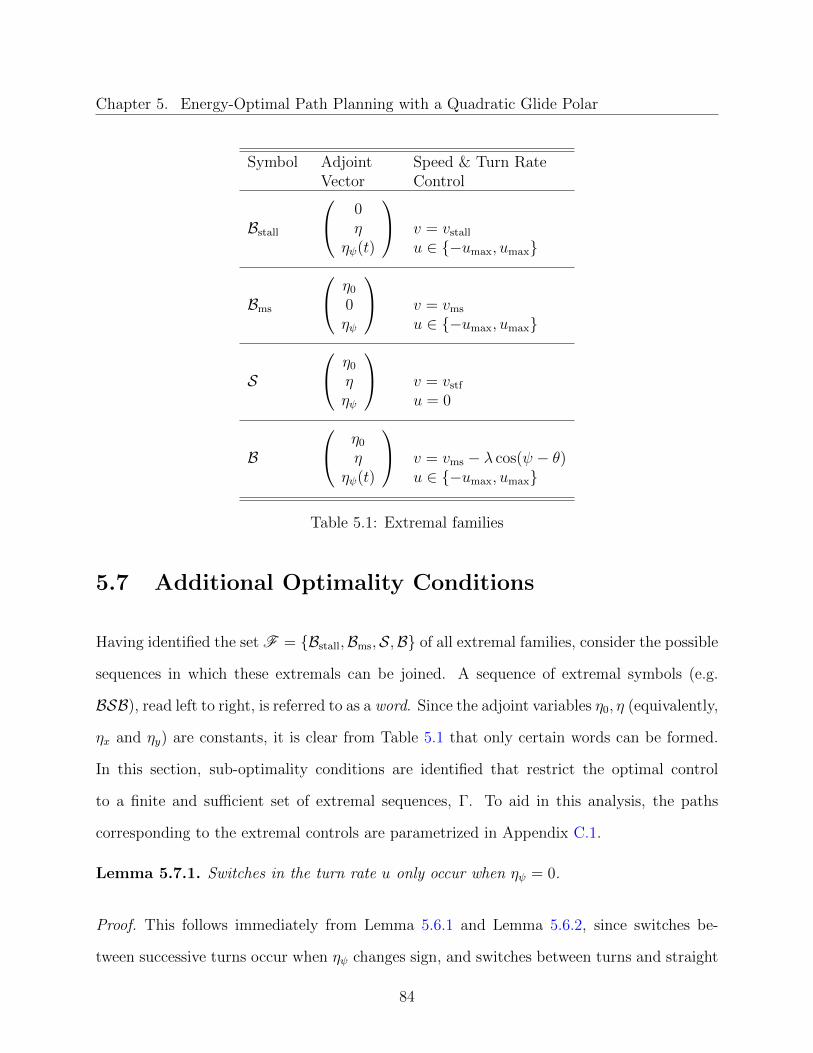
Chapter 5. Energy-Optimal Path Planning with a Quadratic Glide Polar
Symbol AdjointVector
Speed & Turn RateControl
Bstall
0η
ηψ(t)
v = vstall
u ∈ −umax, umax
Bms
η0
0ηψ
v = vms
u ∈ −umax, umax
S
η0
ηηψ
v = vstf
u = 0
B
η0
ηηψ(t)
v = vms − λ cos(ψ − θ)u ∈ −umax, umax
Table 5.1: Extremal families
5.7 Additional Optimality Conditions
Having identified the set F = Bstall,Bms,S,B of all extremal families, consider the possible
sequences in which these extremals can be joined. A sequence of extremal symbols (e.g.
BSB), read left to right, is referred to as a word. Since the adjoint variables η0, η (equivalently,
ηx and ηy) are constants, it is clear from Table 5.1 that only certain words can be formed.
In this section, sub-optimality conditions are identified that restrict the optimal control
to a finite and sufficient set of extremal sequences, Γ. To aid in this analysis, the paths
corresponding to the extremal controls are parametrized in Appendix C.1.
Lemma 5.7.1. Switches in the turn rate u only occur when ηψ = 0.
Proof. This follows immediately from Lemma 5.6.1 and Lemma 5.6.2, since switches be-
tween successive turns occur when ηψ changes sign, and switches between turns and straight
84
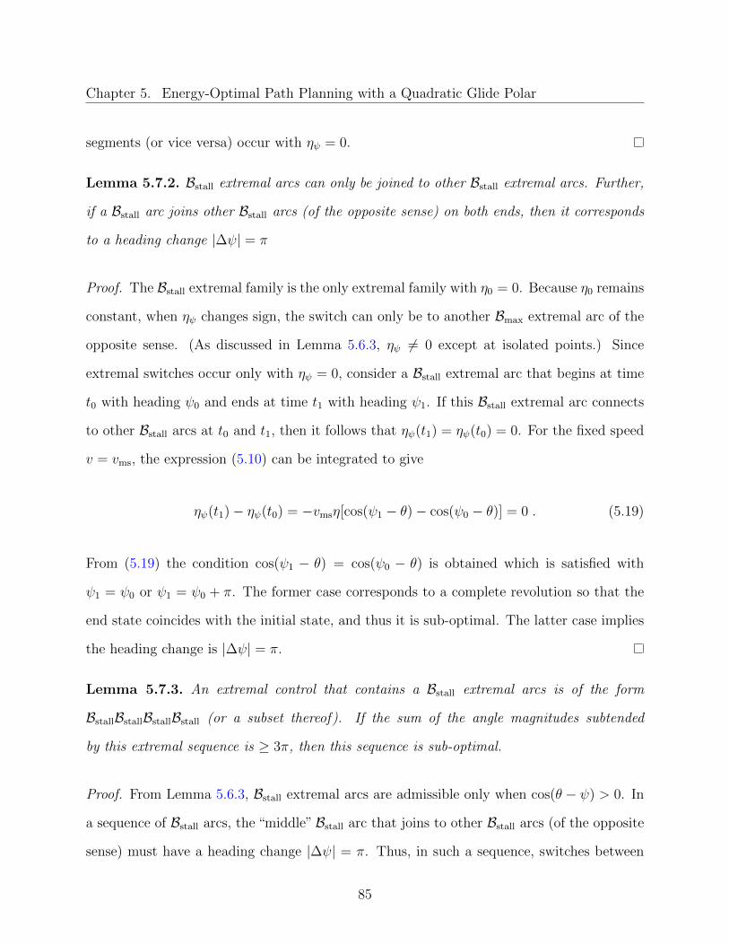
Chapter 5. Energy-Optimal Path Planning with a Quadratic Glide Polar
segments (or vice versa) occur with ηψ = 0.
Lemma 5.7.2. Bstall extremal arcs can only be joined to other Bstall extremal arcs. Further,
if a Bstall arc joins other Bstall arcs (of the opposite sense) on both ends, then it corresponds
to a heading change |∆ψ| = π
Proof. The Bstall extremal family is the only extremal family with η0 = 0. Because η0 remains
constant, when ηψ changes sign, the switch can only be to another Bmax extremal arc of the
opposite sense. (As discussed in Lemma 5.6.3, ηψ 6= 0 except at isolated points.) Since
extremal switches occur only with ηψ = 0, consider a Bstall extremal arc that begins at time
t0 with heading ψ0 and ends at time t1 with heading ψ1. If this Bstall extremal arc connects
to other Bstall arcs at t0 and t1, then it follows that ηψ(t1) = ηψ(t0) = 0. For the fixed speed
v = vms, the expression (5.10) can be integrated to give
ηψ(t1)− ηψ(t0) = −vmsη[cos(ψ1 − θ)− cos(ψ0 − θ)] = 0 . (5.19)
From (5.19) the condition cos(ψ1 − θ) = cos(ψ0 − θ) is obtained which is satisfied with
ψ1 = ψ0 or ψ1 = ψ0 + π. The former case corresponds to a complete revolution so that the
end state coincides with the initial state, and thus it is sub-optimal. The latter case implies
the heading change is |∆ψ| = π.
Lemma 5.7.3. An extremal control that contains a Bstall extremal arcs is of the form
BstallBstallBstallBstall (or a subset thereof). If the sum of the angle magnitudes subtended
by this extremal sequence is ≥ 3π, then this sequence is sub-optimal.
Proof. From Lemma 5.6.3, Bstall extremal arcs are admissible only when cos(θ − ψ) > 0. In
a sequence of Bstall arcs, the “middle”Bstall arc that joins to other Bstall arcs (of the opposite
sense) must have a heading change |∆ψ| = π. Thus, in such a sequence, switches between
85
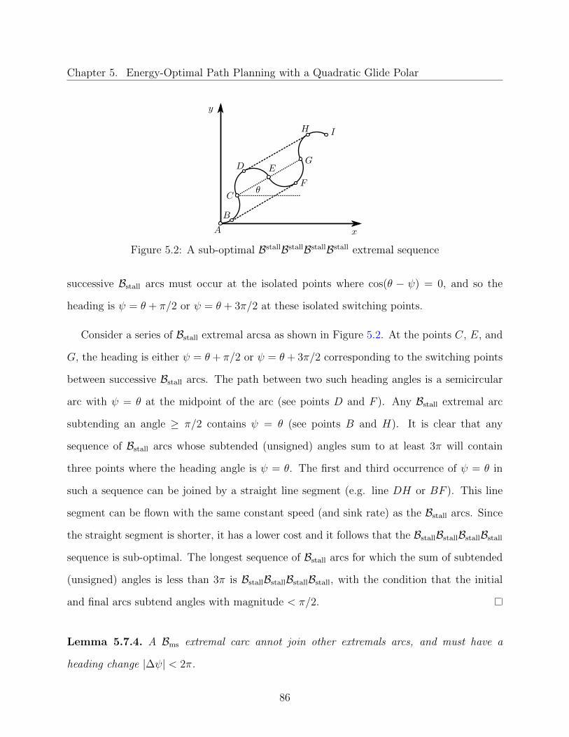
Chapter 5. Energy-Optimal Path Planning with a Quadratic Glide Polar
Figure 5.2: A sub-optimal BstallBstallBstallBstall extremal sequence
successive Bstall arcs must occur at the isolated points where cos(θ − ψ) = 0, and so the
heading is ψ = θ + π/2 or ψ = θ + 3π/2 at these isolated switching points.
Consider a series of Bstall extremal arcsa as shown in Figure 5.2. At the points C, E, and
G, the heading is either ψ = θ+ π/2 or ψ = θ+ 3π/2 corresponding to the switching points
between successive Bstall arcs. The path between two such heading angles is a semicircular
arc with ψ = θ at the midpoint of the arc (see points D and F ). Any Bstall extremal arc
subtending an angle ≥ π/2 contains ψ = θ (see points B and H). It is clear that any
sequence of Bstall arcs whose subtended (unsigned) angles sum to at least 3π will contain
three points where the heading angle is ψ = θ. The first and third occurrence of ψ = θ in
such a sequence can be joined by a straight line segment (e.g. line DH or BF ). This line
segment can be flown with the same constant speed (and sink rate) as the Bstall arcs. Since
the straight segment is shorter, it has a lower cost and it follows that the BstallBstallBstallBstall
sequence is sub-optimal. The longest sequence of Bstall arcs for which the sum of subtended
(unsigned) angles is less than 3π is BstallBstallBstallBstall, with the condition that the initial
and final arcs subtend angles with magnitude < π/2.
Lemma 5.7.4. A Bms extremal carc annot join other extremals arcs, and must have a
heading change |∆ψ| < 2π.
86
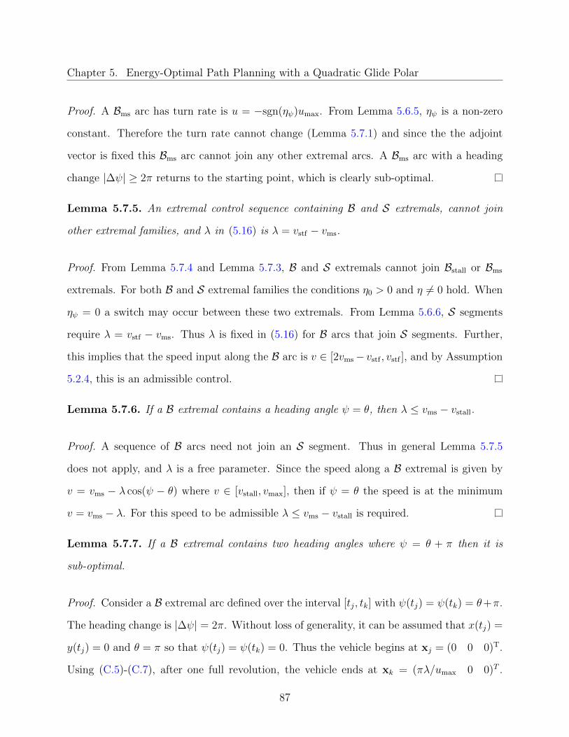
Chapter 5. Energy-Optimal Path Planning with a Quadratic Glide Polar
Proof. A Bms arc has turn rate is u = −sgn(ηψ)umax. From Lemma 5.6.5, ηψ is a non-zero
constant. Therefore the turn rate cannot change (Lemma 5.7.1) and since the the adjoint
vector is fixed this Bms arc cannot join any other extremal arcs. A Bms arc with a heading
change |∆ψ| ≥ 2π returns to the starting point, which is clearly sub-optimal.
Lemma 5.7.5. An extremal control sequence containing B and S extremals, cannot join
other extremal families, and λ in (5.16) is λ = vstf − vms.
Proof. From Lemma 5.7.4 and Lemma 5.7.3, B and S extremals cannot join Bstall or Bms
extremals. For both B and S extremal families the conditions η0 > 0 and η 6= 0 hold. When
ηψ = 0 a switch may occur between these two extremals. From Lemma 5.6.6, S segments
require λ = vstf − vms. Thus λ is fixed in (5.16) for B arcs that join S segments. Further,
this implies that the speed input along the B arc is v ∈ [2vms− vstf , vstf ], and by Assumption
5.2.4, this is an admissible control.
Lemma 5.7.6. If a B extremal contains a heading angle ψ = θ, then λ ≤ vms − vstall.
Proof. A sequence of B arcs need not join an S segment. Thus in general Lemma 5.7.5
does not apply, and λ is a free parameter. Since the speed along a B extremal is given by
v = vms − λ cos(ψ − θ) where v ∈ [vstall, vmax], then if ψ = θ the speed is at the minimum
v = vms − λ. For this speed to be admissible λ ≤ vms − vstall is required.
Lemma 5.7.7. If a B extremal contains two heading angles where ψ = θ + π then it is
sub-optimal.
Proof. Consider a B extremal arc defined over the interval [tj, tk] with ψ(tj) = ψ(tk) = θ+π.
The heading change is |∆ψ| = 2π. Without loss of generality, it can be assumed that x(tj) =
y(tj) = 0 and θ = π so that ψ(tj) = ψ(tk) = 0. Thus the vehicle begins at xj = (0 0 0)T.
Using (C.5)-(C.7), after one full revolution, the vehicle ends at xk = (πλ/umax 0 0)T .
87
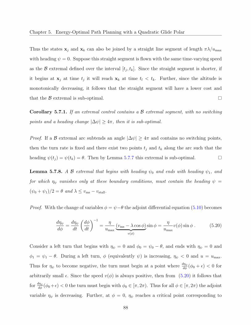
Chapter 5. Energy-Optimal Path Planning with a Quadratic Glide Polar
Thus the states xj and xk can also be joined by a straight line segment of length πλ/umax
with heading ψ = 0. Suppose this straight segment is flown with the same time-varying speed
as the B extremal defined over the interval [tj, tk]. Since the straight segment is shorter, if
it begins at xj at time tj it will reach xk at time tl < tk. Further, since the altitude is
monotonically decreasing, it follows that the straight segment will have a lower cost and
that the B extremal is sub-optimal.
Corollary 5.7.1. If an extremal control contains a B extremal segment, with no switching
points and a heading change |∆ψ| ≥ 4π, then it is sub-optimal.
Proof. If a B extremal arc subtends an angle |∆ψ| ≥ 4π and contains no switching points,
then the turn rate is fixed and there exist two points tj and tk along the arc such that the
heading ψ(tj) = ψ(tk) = θ. Then by Lemma 5.7.7 this extremal is sub-optimal.
Lemma 5.7.8. A B extremal that begins with heading ψ0 and ends with heading ψ1, and
for which ηψ vanishes only at these boundary conditions, must contain the heading ψ =
(ψ0 + ψ1)/2 = θ and λ ≤ vms − vstall.
Proof. With the change of variables φ = ψ−θ the adjoint differential equation (5.10) becomes
dηψdφ
=dηψdt
(dφ
dt
)−1
=η
umax
(vms − λ cosφ)︸ ︷︷ ︸v(φ)
sinφ =η
umax
v(φ) sinφ . (5.20)
Consider a left turn that begins with ηψ = 0 and φ0 = ψ0 − θ, and ends with ηψ = 0 and
φ1 = ψ1 − θ. During a left turn, φ (equivalently ψ) is increasing, ηψ < 0 and u = umax.
Thus for ηψ to become negative, the turn must begin at a point wheredηψdφ
(φ0 + ε) < 0 for
arbitrarily small ε. Since the speed v(φ) is always positive, then from (5.20) it follows that
fordηψdφ
(φ0 +ε) < 0 the turn must begin with φ0 ∈ [π, 2π). Thus for all φ ∈ [π, 2π) the adjoint
variable ηψ is decreasing. Further, at φ = 0, ηψ reaches a critical point corresponding to
88
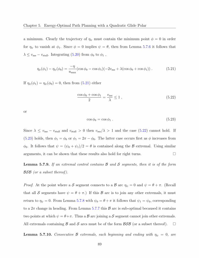
Chapter 5. Energy-Optimal Path Planning with a Quadratic Glide Polar
a minimum. Clearly the trajectory of ηψ must contain the minimum point φ = 0 in order
for ηψ to vanish at φ1. Since φ = 0 implies ψ = θ, then from Lemma 5.7.6 it follows that
λ ≤ vms − vstall. Integrating (5.20) from φ0 to φ1 ,
ηψ(φ1)− ηψ(φ0) =−ηumax
(cosφ0 − cosφ1)(−2vms + λ(cosφ0 + cosφ1)) . (5.21)
If ηψ(φ1) = ηψ(φ0) = 0, then from (5.21) either
cosφ0 + cosφ1
2=vms
λ≤ 1 , (5.22)
or
cosφ0 = cosφ1 . (5.23)
Since λ ≤ vms − vstall and vstall > 0 then vms/λ > 1 and the case (5.22) cannot hold. If
(5.23) holds, then φ1 = φ0 or φ1 = 2π − φ0. The latter case occurs first as φ increases from
φ0. It follows that ψ = (ψ0 + ψ1)/2 = θ is contained along the B extremal. Using similar
arguments, it can be shown that these results also hold for right turns.
Lemma 5.7.9. If an extremal control contains B and S segments, then it is of the form
BSB (or a subset thereof).
Proof. At the point where a S segment connects to a B arc ηψ = 0 and ψ = θ + π. (Recall
that all S segments have ψ = θ + π.) If this B arc is to join any other extremals, it must
return to ηψ = 0. From Lemma 5.7.8 with ψ0 = θ+ π it follows that ψ1 = ψ0, corresponding
to a 2π change in heading. From Lemma 5.7.7 this B arc is sub-optimal becaused it contains
two points at which ψ = θ+π. Thus a B arc joining a S segment cannot join other extremals.
All extremals containing B and S arcs must be of the form BSB (or a subset thereof).
Lemma 5.7.10. Consecutive B extremals, each beginning and ending with ηψ = 0, are
89
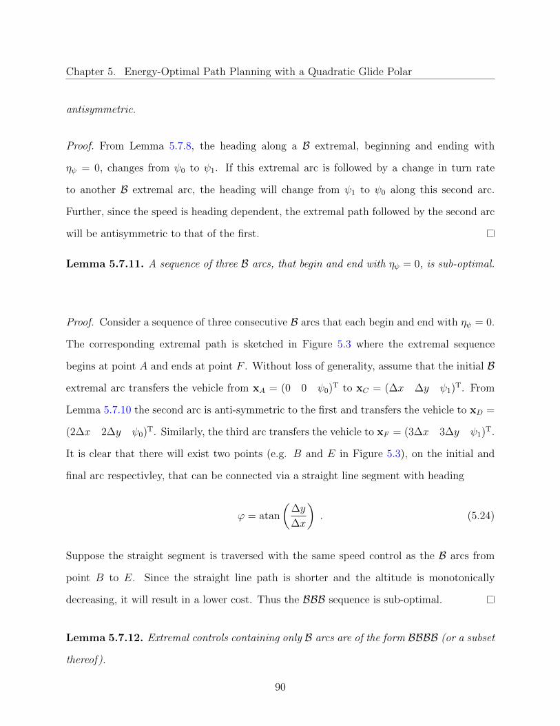
Chapter 5. Energy-Optimal Path Planning with a Quadratic Glide Polar
antisymmetric.
Proof. From Lemma 5.7.8, the heading along a B extremal, beginning and ending with
ηψ = 0, changes from ψ0 to ψ1. If this extremal arc is followed by a change in turn rate
to another B extremal arc, the heading will change from ψ1 to ψ0 along this second arc.
Further, since the speed is heading dependent, the extremal path followed by the second arc
will be antisymmetric to that of the first.
Lemma 5.7.11. A sequence of three B arcs, that begin and end with ηψ = 0, is sub-optimal.
Proof. Consider a sequence of three consecutive B arcs that each begin and end with ηψ = 0.
The corresponding extremal path is sketched in Figure 5.3 where the extremal sequence
begins at point A and ends at point F . Without loss of generality, assume that the initial B
extremal arc transfers the vehicle from xA = (0 0 ψ0)T to xC = (∆x ∆y ψ1)T. From
Lemma 5.7.10 the second arc is anti-symmetric to the first and transfers the vehicle to xD =
(2∆x 2∆y ψ0)T. Similarly, the third arc transfers the vehicle to xF = (3∆x 3∆y ψ1)T.
It is clear that there will exist two points (e.g. B and E in Figure 5.3), on the initial and
final arc respectivley, that can be connected via a straight line segment with heading
ϕ = atan
(∆y
∆x
). (5.24)
Suppose the straight segment is traversed with the same speed control as the B arcs from
point B to E. Since the straight line path is shorter and the altitude is monotonically
decreasing, it will result in a lower cost. Thus the BBB sequence is sub-optimal.
Lemma 5.7.12. Extremal controls containing only B arcs are of the form BBBB (or a subset
thereof).
90

Chapter 5. Energy-Optimal Path Planning with a Quadratic Glide Polar
Figure 5.3: The sequence of three B extremal arcs, that each begin and end with ηψ = 0, issub-optimal
Proof. In a sequence of B arcs, the B arcs that connect to other B arcs at both ends (i.e., the
interior B arcs in BBBB) are required to begin and end with ηψ = 0. Thus they satisfy the
conditions of Lemma 5.7.10 and Lemma 5.7.11. However, the initial and final B arcs that join
a boundary condition (i.e. the first and last B arcs in BBBB) do not necessarily satisfy these
same properties. (These B arcs may be be truncated to satisfy the boundary conditions.)
Thus the longest sequence of B extremals, in terms of the number of extremals, is of the
form BBBB with the restriction that the initial and final B arcs are sufficiently short, such
that they do not contain heading angles ψ = ϕ given in (5.24). The same restriction applies
to a BBB extremal sequence. Such sequences also require that the constant λ ≤ vms − vstall
by Lemma 5.7.8.
If the extremal sequence is of the form BB or B then Lemma 5.7.10 and Lemma 5.7.11
do not apply. In this case λ is restricted such that for all the heading angles traversed
v = vms − λ cos(ψ − θ) ∈ [vstall, vmax]. A BB sequence will contain at least one point where
ηψ = 0 (corresponding to the switching point). Whereas a B arc is not required to contain
91

Chapter 5. Energy-Optimal Path Planning with a Quadratic Glide Polar
the point ηψ = 0.
For brevity, the word BBBB is used to denote all of these extremal sequences (including
those of the form BBB, BB, and B), recognizing that for each sequence there are unique
constraints on the extremal arcs.
Theorem 5.7.1. The set
Γ = BSB, BBBB, Bms, BstallBstallBstallBstall (5.25)
of extremal controls contains the optimal control.
Proof. In Theorem 5.6.1 it was shown that the set F = Bstall,Bms,S,B contains all ex-
tremal families. In Lemma 5.7.3 it was shown that all extremal controls containing Bstall arcs
are of the form BstallBstallBstallBstall (or a subset thereof). In Lemma 5.7.4 it was shown that
Bms extremals cannot join other extremals. In Lemma 5.7.9 it was shown that if an extremal
control contains B and S segments, then it is of the form BSB (or a subset thereof). Last,
in Lemma 5.7.12, it was shown that extremal controls containing only B arcs are of the form
BBBB (or a subset thereof). Thus it follows that Γ is a finite and sufficient set of candidate
extremal controls. It has been established in Section 5.4 that an optimal control exists, and
therefore Γ contains the optimal control.
5.8 Path Synthesis
The set Γ contains all of the extremal control sequences that are candidates for an optimal
control. Each member of Γ is referred to as a class of candidate controls. In Appendix C.1
individual extremals are parametrized to describe their resulting planar displacements and
heading changes. Similarly, each class of controls in Γ can be parametrized to give the glider’s
92

Chapter 5. Energy-Optimal Path Planning with a Quadratic Glide Polar
final state resulting from the corresponding extremal sequence. The space of parameters
admissible for a given class and path type is denoted as P . The path synthesis problem is
to determine the optimal control history u∗(·) (equivalently, the class in Γ and parameter
p ∈ P ) that minimizes the cost while satisfying the boundary conditions.
For a given class, solutions satisfying the boundary conditions may exist at several iso-
lated points or neighborhoods in the parameter space. If the solutions exist at several
isolated points, path synthesis is similar to a root finding problem. If there exists continu-
ously parametrized sets of solutions, the lowest cost “locally” optimal solution within each
neighborhood is sought. Intuitively, one might expect that these locally optimal controls cor-
respond to paths that are qualitatively distinct. (Paths within a class may be qualitatively
distinct, for example, if the orientation or a number of extremals they contain are unique.)
Consider the class of BSB candidate optimal controls. If left turns are denoted with the
symbol L, right turns with R, and straight segments with S, then the set LSL,LSR,RSL,
RSR contains all the possible orientations of a BSB control. In this case, the boundary
conditions may be satisfied by several paths corresponding to different orientations. (For
example, if the final endpoint is on the negative x-axis with heading ψ = π then, by sym-
metry, any path to the endpoint can be reflected about the x-axis to obtain a path with the
same cost but with a different orientation.) Similarly, controls in the classes BBBB, Bms or
BstallBstallBstallBstall may either begin with a right (R) or left (L) turn and successive turns
are of the opposite sense. Therefore there are two orientations to consider in these cases. If
a particular extremal within a class has zero length then the corresponding control is unique
in terms of the number (and sequence) of extremals. For example, if the BSB sequence
contains one or more extremals of zero length, the controls may be of the form BS, SB, BB,
B or S.
One approach to solving the path synthesis problem is to enumerate all of solutions that
93

Chapter 5. Energy-Optimal Path Planning with a Quadratic Glide Polar
satisfy the boundary conditions for each candidate class in Γ, and then compare their respec-
tive costs. In the case of a particular class having a neighborhood of solutions that satisfy
the boundary conditions the locally optimal solution is sought. A numerical rootfinding and
optimization routine that enumerates all such solutions would always give the globally opti-
mal control (accurate to within a user specified tolerance). In practice however, it is difficult
to construct such an algorithm. One may therefore expect only locally optimal paths, in
general. In Appendix C a method for computing the candidate controls for each class in Γ
is presented. The BSB controls can be easily computed by solving a root finding problem in
one parameter, as shown in Appendix C.2. The class of BBBB paths is parametrized with
more unknown variables than constraints and a unique solution is not available. Thus, in
Appendix C.3, a constrained optimization problem is formulated to solve for the parameter
vector p in this case. Last, in Appendix C.4 it is shown that the parameters of Bms or
BstallBstallBstallBstall extremals can be found algebraically (when they exist).
5.9 Illustrative Examples
To illustrate the path synthesis procedure, a glider model that is representative of the DG-
1001M motorglider is assumed. (This is a modern optionally powered glider, with a 20 meter
wingspan, manufactured by DG Flugzeugbau in Germany.) The glide polar curve given in the
DG-1001M flight manual DG Flugzeugbau Gmbh (2010), corresponding to a wing loading of
35 kg/m2, was digitized and is indicated by the dashed line in Figure 5.4. A quadratic curve
was fit to this data to give an approximate glide polar (solid line in Figure 5.4) expressed by
the function:
w(v) = 0.0002093︸ ︷︷ ︸a
v2−0.0381︸ ︷︷ ︸b
v + 2.3146︸ ︷︷ ︸c
, (5.26)
94

Chapter 5. Energy-Optimal Path Planning with a Quadratic Glide Polar
80 100 120 140 1600.5
0.6
0.7
0.8
0.9
1
1.1
1.2
1.3
1.4
1.5
Speedlxkph)
Sin
klR
atel
xm/s
)
DG−1001MlGlidelPolarQuadraticlApproximation
Figure 5.4: Digitized glide polar of the DG-1001M motorglider (dashed line), adapted fromDG Flugzeugbau Gmbh (2010), compared to a quadratic approximation (solid line)
where the units of sink rate w are in meters/second and the units of speed v are in kph
(kilometers/hour). Since the previous analysis showed that the extremal controls are confined
to the speed interval v ∈ [vstall, vstf ], only a subset of the available data was used for curve
fitting. A data set was chosen that resulted in the smallest error between the approximate
and actual stall, minimum sink and best glide flight conditions. Since flying at the stall
speed is not desirable, and since this stall region deviates significantly from the parabolic
shape of the remaining glide polar, the stall speed was artificially increased to vstall = 75.6
kph. This is a more realistic minimum operating speed, and the quadratic glide polar is a
better approximation of the data with this conservative assumption. The speed and sink
rates at these various flight conditions are indicated with circle markers for actual values
and square markers for approximate values in Figure 5.4. The corresponding numeric values
for these flight conditions are given in Table 5.2. With this tabulated data one may verify
that Assumption 5.2.4 is satisfied by the quadratic approximation. (It is also satisfied by the
actual glide polar if the actual stall speed is used.)
95

Chapter 5. Energy-Optimal Path Planning with a Quadratic Glide Polar
Flight Condition ActualSpeed(kph)
Approx.Speed(kph)
ActualSink Rate(m/s)
Approx.Sink Rate(m/s)
Stall Speed 75.6 75.6 0.66 0.63
Minimum Sink 88.0 91.1 0.56 0.58
Speed to Fly 104.0 105.2 0.62 0.62
Table 5.2: Comparison of approximate and actual speeds and sink rates at various flightconditions
As discussed in Remark 5.2.1, the glide polar w(v) is assumed to be independent of the
turn rate u. This approximation is only valid for mild turns with very shallow bank angles.
For the DG-1001M the turn rate limit is assumed to be umax = π/15 (radians/sec) (i.e., it
takes 15 seconds to complete a turn with a 180 degree heading change). For the kinematic car
model the minimum turn radius R scales with the speed: R = v/umax. Thus the approximate
minimum turn radius at the speed to fly is about Rstf = 139 m, and at the stall speed the
radius is about Rstall = 100 m. Note that the change in sink rate on the interval [vmin, vstf ] is
very small compared to the changes in speed and turn radius. Over large distances a small
change in sink rate may become significant, however on the scale of a few hundred meters
these effects are not as pronounced. Instead, the altitude loss is largely influenced by the
transit time to the goal. Intuitively, one might think that strictly operating at the speed to
fly will minimize the altitude loss to the goal. However, the advantage of slowing down is
that the minimum turning radius decreases, potentially allowing a shorter and faster path
to the goal; with a smaller turn radius the reduction in transit time may be large enough to
justify the penalty incurred by a small increase in sink rate.
To demonstrate the path synthesis algorithm three final endpoints were selected. The
resulting candidate paths are plotted, and their costs are compared (see Figure 5.5(a),5.6(a)
and 5.7(a)). In each case the glider begins at the origin, pointed east along the x axis with
96

Chapter 5. Energy-Optimal Path Planning with a Quadratic Glide Polar
−2 −1 0 1 2 3−2
−1
0
1
2
3
x
y
(a) Candidate paths
0 5 10 15 20 25 30−0.2
−0.1
0
0.1
0.2
Time, s
Tur
n R
ate,
rad
/s
0 5 10 15 20 25 30
80
90
100
Time, sS
peed
, kph
(b) Optimal control history
Figure 5.5: Path synthesis result for the normalized final state x1 = (0 1 2π/3)T
x0 = (0 0 0)T and the candidate paths to the endpoint x1 are labeled with their path
type, orientation, and cost. (The cost is altitude loss in meters and is given in square brackets
next to each path.) For comparison, the Dubins path at the speed to fly is plotted in each
case with a dashed line. Note that the x and y axes have been normalized by the turn radius
at the speed to fly Rstf . Further, the optimal control history corresponding to the lowest
cost path in each case is given in the adjacent plots (see Figure 5.5(b),5.6(b) and 5.7(b)).
The turn rate limits and the speed limits at vstall and vstf are plotted with dashed lines.
In Figure 5.5 the endpoint is x1 = (0 1 2π/3)T and the lowest cost control is of the type
BBB, with orientation RLR. Since this endpoint is very close to the initial state, significant
maneuvering is required. In comparison to the Dubins path the altitude loss is reduced by 2.4
meters which is an 11% improvement. From the optimal control history in Figure 5.5(b), the
glider speed changes drastically and reaches the minimum speed (and smallest turn radius)
in the middle of the second turn.
In Figure 5.6 the endpoint is x1 = (−3 4 0)T and the lowest cost control is of the type
97

Chapter 5. Energy-Optimal Path Planning with a Quadratic Glide Polar
−6 −5 −4 −3 −2 −1 0 1 2−2
−1
0
1
2
3
4
5
6
x
y
(a) Candidate paths
0 5 10 15 20 25 30 35 40−0.2
−0.1
0
0.1
0.2
Time, s
Tur
n R
ate,
rad
/s
0 5 10 15 20 25 30 35 40
80
90
100
Time, sS
peed
, kph
(b) Optimal control history
Figure 5.6: Path synthesis result for the normalized final state x1 = (−3 4 0)T
BSB, with orientation LSR. Since the endpoint is relatively far from the starting point, it
cannot be reached by a BBBB candidate control. For endpoints that are sufficiently far away,
all candidate controls in Γ need not be computed; only controls of the class BSB should be
considered. In this case, the altitude loss is reduced by about 1.8 m or 6.5% relative to
the Dubins path. Note the smooth transition in the speed control between the B and S
extremals as shown in Figure 5.6(b).
Last, in Figure 5.7 the endpoint is x1 = (0 2 7π/4)T and the lowest cost control is of
the type BSB, with orientation LSL. It is interesting to note that the orientation of the
Dubins path is also LSL. In this case the the altitude loss is reduced by about 1.7 m or
7.8% relative to the Dubins path.
98

Chapter 5. Energy-Optimal Path Planning with a Quadratic Glide Polar
−3 −2 −1 0 1 2 3−2
−1
0
1
2
3
4
x
y
(a) Candidate paths
0 5 10 15 20 25 30−0.2
−0.1
0
0.1
0.2
Time, s
Tur
n R
ate,
rad
/s
0 5 10 15 20 25 30
80
90
100
Time, sS
peed
, kph
(b) Optimal control history
Figure 5.7: Path synthesis result for the normalized final state x1 = (0 2 7π/4)T
5.10 Conclusion
The problem of minimizing altitude loss for a sailplane maneuvering in still air to a nearby
position and heading angle was investigated. The glider was modeled as a Dubins car with a
sink rate that is a quadratic function of the speed. The extremal controls were found to con-
sist of straight segments flown at the best glide speed (denoted as S extremals) and maximum
rate turns with either: a heading dependent speed input (B extremals), the stall speed (Bstall
extremals), or the minimum sink speed (Bms extremals). The optimal control was found to
be a member of the finite and sufficient set Γ = BSB, BBBB, BstallBstallBstallBstall, Bms. A
path synthesis procedure was proposed to numerically solve for each candidate path in Γ, and
to identify the lowest cost (locally) optimal control. An illustrative example, based on the
DG-1001M motorglider, demonstrated a significant improvement in altitude loss resulting
from the proposed approach when compared to a standard Dubins path planning algorithm
(with a fixed speed for best wings-level glide). One limitation of the proposed approach,
however, is that it has been assumed that sink rate does not vary with turn rate. The pro-
99

Chapter 5. Energy-Optimal Path Planning with a Quadratic Glide Polar
posed algorithm is therefore appropriate for shallow, banked turns where the quadratic glide
polar is a reasonable approximation.
100

Chapter 6
Energy-Optimal Path Planning with
Speed and Load Factor Controls
6.1 Introduction
In Chapter 5 the path planning problem of minimizing change in depth (equivalently, altitude
loss for a sailplane) was considered. The Dubins car motion model (2.10) was modified
such that the speed could vary within a strictly positive interval. The “glide polar” (sink
rate versus speed) was approximated as a quadratic (in speed) function. One advantage
of using this approximation was that the reduction in complexity of the problem makes
it easier to characterize the extremals analytically. In particular, a finite and sufficient
set of candidate extremal control sequences was identified, and a numerial root finding (or
constrained optimization) routine was proposed for finding each candidate control. However,
since the glide polar is assumed to be independent of the turn rate, these results are restricted
to shallow bank angles. Here this problem is revisited with this restriction removed; physics-
based turn rate and sink rate models are developed in which the speed and load factor controls
101

Chapter 6. Energy-Optimal Path Planning with Speed and Load Factor Controls
are coupled. Such energy-turn analysis provides a link between load-factor, turn-rate and
energy-rate; see (Cliff et al., 1982, 1992; Halter and Cliff, 1991) for related discussions.
The following work is adapted from (Wolek et al., 2015a).
6.2 Gliding and Turning Flight
Consider the free body diagram of a glider in a steady turn at speed V and bank angle φ,
as shown in Figures 6.1 and 6.2. For a glider with buoyancy B, define the net weight
Figure 6.1: Longitudinal forces in a steady gliding turn
acting on the vehicle as W = B −W = εW where W = mg is the “dry weight” (with mass
m and gravitational acceleration g) and where ε ≤ 1 is the ratio of the net weight to dry
weight. Referring to Figures 6.1 and 6.2 and summing the net weight W , lift L, drag D,
Figure 6.2: Lateral forces in a steady gliding turn
102
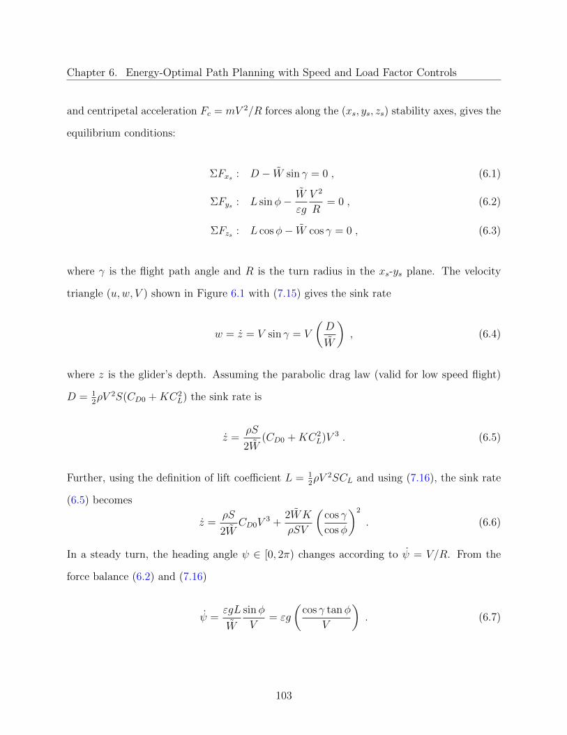
Chapter 6. Energy-Optimal Path Planning with Speed and Load Factor Controls
and centripetal acceleration Fc = mV 2/R forces along the (xs, ys, zs) stability axes, gives the
equilibrium conditions:
ΣFxs : D − W sin γ = 0 , (6.1)
ΣFys : L sinφ− W
εg
V 2
R= 0 , (6.2)
ΣFzs : L cosφ− W cos γ = 0 , (6.3)
where γ is the flight path angle and R is the turn radius in the xs-ys plane. The velocity
triangle (u,w, V ) shown in Figure 6.1 with (7.15) gives the sink rate
w = z = V sin γ = V
(D
W
), (6.4)
where z is the glider’s depth. Assuming the parabolic drag law (valid for low speed flight)
D = 12ρV 2S(CD0 +KC2
L) the sink rate is
z =ρS
2W(CD0 +KC2
L)V 3 . (6.5)
Further, using the definition of lift coefficient L = 12ρV 2SCL and using (7.16), the sink rate
(6.5) becomes
z =ρS
2WCD0V
3 +2WK
ρSV
(cos γ
cosφ
)2
. (6.6)
In a steady turn, the heading angle ψ ∈ [0, 2π) changes according to ψ = V/R. From the
force balance (6.2) and (7.16)
ψ =εgL
W
sinφ
V= εg
(cos γ tanφ
V
). (6.7)
103
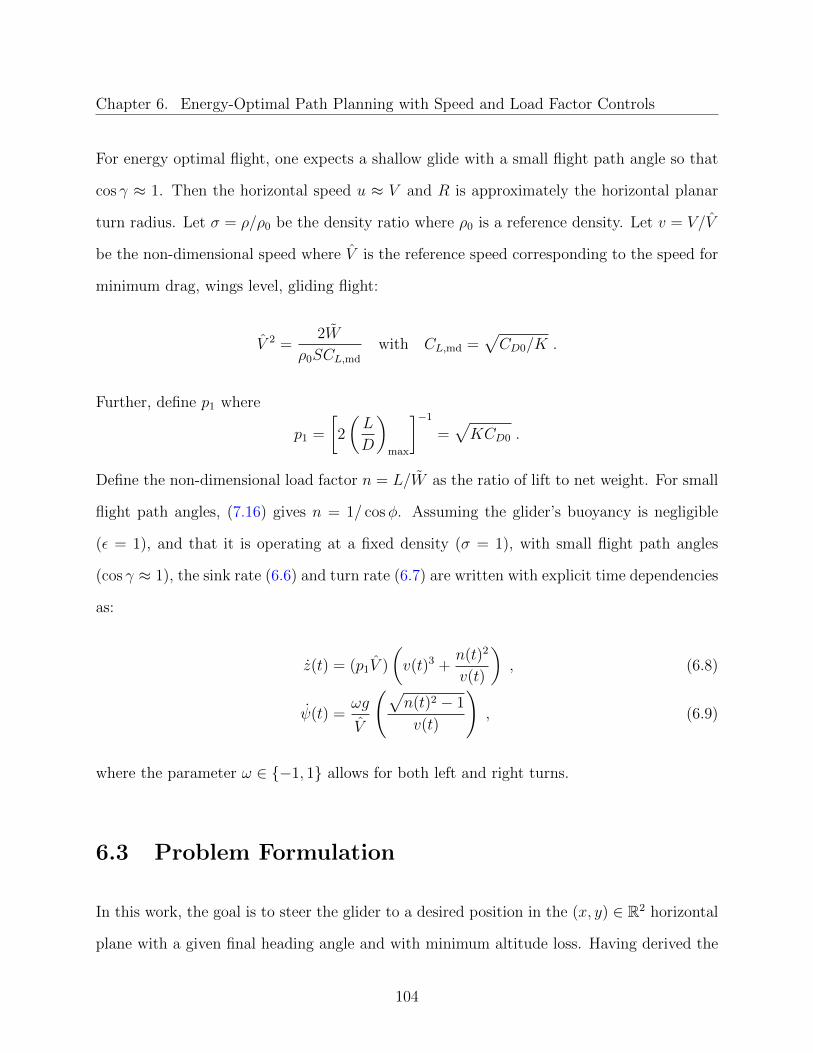
Chapter 6. Energy-Optimal Path Planning with Speed and Load Factor Controls
For energy optimal flight, one expects a shallow glide with a small flight path angle so that
cos γ ≈ 1. Then the horizontal speed u ≈ V and R is approximately the horizontal planar
turn radius. Let σ = ρ/ρ0 be the density ratio where ρ0 is a reference density. Let v = V/V
be the non-dimensional speed where V is the reference speed corresponding to the speed for
minimum drag, wings level, gliding flight:
V 2 =2W
ρ0SCL,md
with CL,md =√CD0/K .
Further, define p1 where
p1 =
[2
(L
D
)max
]−1
=√KCD0 .
Define the non-dimensional load factor n = L/W as the ratio of lift to net weight. For small
flight path angles, (7.16) gives n = 1/ cosφ. Assuming the glider’s buoyancy is negligible
(ε = 1), and that it is operating at a fixed density (σ = 1), with small flight path angles
(cos γ ≈ 1), the sink rate (6.6) and turn rate (6.7) are written with explicit time dependencies
as:
z(t) = (p1V )
(v(t)3 +
n(t)2
v(t)
), (6.8)
ψ(t) =ωg
V
(√n(t)2 − 1
v(t)
), (6.9)
where the parameter ω ∈ −1, 1 allows for both left and right turns.
6.3 Problem Formulation
In this work, the goal is to steer the glider to a desired position in the (x, y) ∈ R2 horizontal
plane with a given final heading angle and with minimum altitude loss. Having derived the
104
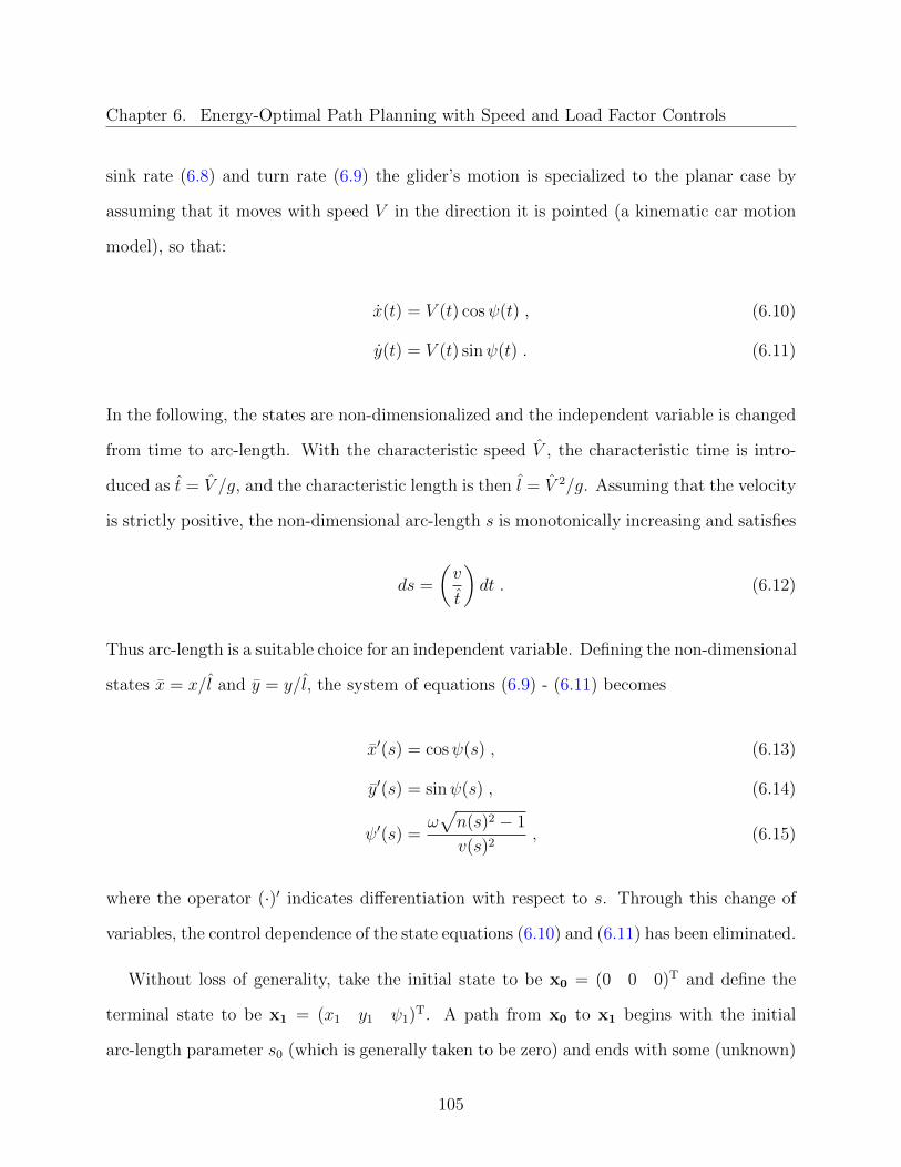
Chapter 6. Energy-Optimal Path Planning with Speed and Load Factor Controls
sink rate (6.8) and turn rate (6.9) the glider’s motion is specialized to the planar case by
assuming that it moves with speed V in the direction it is pointed (a kinematic car motion
model), so that:
x(t) = V (t) cosψ(t) , (6.10)
y(t) = V (t) sinψ(t) . (6.11)
In the following, the states are non-dimensionalized and the independent variable is changed
from time to arc-length. With the characteristic speed V , the characteristic time is intro-
duced as t = V /g, and the characteristic length is then l = V 2/g. Assuming that the velocity
is strictly positive, the non-dimensional arc-length s is monotonically increasing and satisfies
ds =
(v
t
)dt . (6.12)
Thus arc-length is a suitable choice for an independent variable. Defining the non-dimensional
states x = x/l and y = y/l, the system of equations (6.9) - (6.11) becomes
x′(s) = cosψ(s) , (6.13)
y′(s) = sinψ(s) , (6.14)
ψ′(s) =ω√n(s)2 − 1
v(s)2, (6.15)
where the operator (·)′ indicates differentiation with respect to s. Through this change of
variables, the control dependence of the state equations (6.10) and (6.11) has been eliminated.
Without loss of generality, take the initial state to be x0 = (0 0 0)T and define the
terminal state to be x1 = (x1 y1 ψ1)T. A path from x0 to x1 begins with the initial
arc-length parameter s0 (which is generally taken to be zero) and ends with some (unknown)
105

Chapter 6. Energy-Optimal Path Planning with Speed and Load Factor Controls
final arc-length s1. Thus the initial conditions are given by
x(s0) = x0 . (6.16)
The controls inputs (v, n) are subject to bounds. The load factor varies from unity (wings
level gliding flight) to nmax > 1 (flight with maximum bank angle, typically corresponding
to a structural or actuator limit). Thus a constraint is:
1 ≤ n ≤ nmax . (6.17)
The speed is constrained by the stall boundary (CL ≤ CLmax) so that:
n ≤ p2v2 , (6.18)
where p2 = CLmax/CLmd> 1. Equivalently, p2 = 1/v2
min where vmin is the non-dimensional
minimum (stall) speed in wings level flight. Last, the maximum speed constraint is:
v ≤ vmax . (6.19)
At a given arc-length s ∈ [s0, s1] the available inputs u(s) = (v(s), n(s)) are confined to the
control constraint set
Ω =
(v, n) ∈ R2 | 1 ≤ n ≤ nmax, n ≤ p2v2 and v ≤ vmax
. (6.20)
A sample v-n diagram depicting Ω is shown in Figure 6.3 for the parameters:
nmax = 2,
(L
D
)max
= 30, vmin = 0.75, vmax = 2 . (6.21)
106
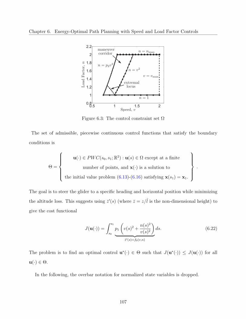
Chapter 6. Energy-Optimal Path Planning with Speed and Load Factor Controls
0.5 1 1.5 20.8
1
1.2
1.4
1.6
1.8
2
2.2
Figure 6.3: The control constraint set Ω
The set of admissible, piecewise continuous control functions that satisfy the boundary
conditions is
Θ =
u(·) ∈ PWC(s0, s1;R2) : u(s) ∈ Ω except at a finite
number of points, and x(·) is a solution to
the initial value problem (6.13)-(6.16) satisfying x(s1) = x1.
.
The goal is to steer the glider to a specific heading and horizontal position while minimizing
the altitude loss. This suggests using z′(s) (where z = z/l is the non-dimensional height) to
give the cost functional
J(u(·)) =
∫ s1
s0
p1
(v(s)2 +
n(s)2
v(s)2
)︸ ︷︷ ︸
z′(s)=f0(v,n)
ds. (6.22)
The problem is to find an optimal control u∗(·) ∈ Θ such that J(u∗(·)) ≤ J(u(·)) for all
u(·) ∈ Θ.
In the following, the overbar notation for normalized state variables is dropped.
107

Chapter 6. Energy-Optimal Path Planning with Speed and Load Factor Controls
6.4 Applying the Minimum Principle
To apply the Minimum Principle, introduce the variational Hamiltonian
H(η0, ~η, x, y, ψ, v, n) = η0f0(n, v) + 〈~η, ~f(ψ, v, n)〉
= η0p1
(v2 +
n2
v2
)+ ηx cosψ + ηy sinψ + ηψ
(ω√n2 − 1
v2
),
where ~f(ψ, v, n) = (fx fy fψ)T is the right hand side of the state-system (6.13)-(6.15),
and ~η = (ηx ηy ηψ)T is a vector of corresponding adjoint variables. The term f0(v, n) is the
integrand of the cost functional (6.22) and η0 is the associated adjoint variable. The Minimum
Principle states that if a control pair (v∗, n∗) is optimal, then there exists a constant η0 ≥ 0
and absolutely continuous functions ηx, ηy and ηψ such that
η′x = −∂H∂x
= 0 , (6.23)
η′y = −∂H∂y
= 0 , (6.24)
η′ψ = −∂H∂ψ
= ηx sinψ − ηy cosψ . (6.25)
(The Minimum Principle does not admit a trivial solution to (6.23) - (6.25), and ηx and ηy
remain constant because the states x and y do not appear in the Hamiltonian.) Moreover,
min(v,n)∈Ω
H(η∗0, ~η∗, x∗, y∗, ψ∗, v, n) = H(η∗0, ~η
∗, x∗, y∗, ψ∗, v∗, n∗) = 0 .
That is, the Hamiltonian is minimized with the optimal controls and is equal to zero along
the optimal trajectory. Recalling that the adjoint variables ηx and ηy are constant, then
ηx = η cos θ, ηy = η sin θ ,
108

Chapter 6. Energy-Optimal Path Planning with Speed and Load Factor Controls
for some constants η and θ, so that the differential equation (6.25) can be rewritten as
η′ψ = η sin(ψ − θ) , (6.26)
and the variational Hamiltonian as
H = η0p1
(v2 +
n2
v2
)+ ηψ
(ω√n2 − 1
v2
)︸ ︷︷ ︸
Hc(η0,ηψ ,v,n)
+η cos(ψ − θ) , (6.27)
where Hc(η0, ηψ, v, n) is the control dependent part of the Hamiltonian.
6.5 Geometrical Approach - the Hodograph
The control dependent part Hc of the Hamiltonian (6.27) is given by
Hc =
⟨ ηψ
η0
,
fψ(v, n)
f0(v, n)
⟩
= η0 p1
(v2 +
n2
v2
)︸ ︷︷ ︸
f0(v,n)
+ηψω√n2 − 1
v2︸ ︷︷ ︸fψ(v,n)
. (6.28)
Equation (6.28) suggests examining the set of attainable (state and cost) rates(fψ(v,n)
f0(v,n)
)where (v, n) varies over the constraint set Ω. Values that minimize the inner product (6.28)
will minimize H. The image of Ω under(fψ(v,n)
f0(v,n)
),
109

Chapter 6. Energy-Optimal Path Planning with Speed and Load Factor Controls
(fψ(v, n)f0(v, n)
): Ω→ I(Ω) ⊂ R2 , (6.29)
is the hodograph set. Because this two-dimensional map is independent of the state, the
image can be graphed in terms of cost-rate (f0, the sink rate) and state-rate (fψ, the turn
rate). This is shown in Figure 6.4 for the parameters (6.21). Referring to Figure 6.3, the
boundaries of Ω map to the boundaries of the hodograph with the exception of the stall
boundary (which only partially maps to the boundary of the hodograph). The southern
boundary of the hodograph corresponds to an extremal locus on the interior of Ω. (This
extremal locus shall be derived in the following section.) The attainable rates of interest
in the hodograph set are those vectors(fψ(v,n)
f0(v,n)
)that minimize Hc for a given vector ( ηψη0 ).
Referring to (6.28), note that Hc = 0 along the line through the origin that is orthogonal
to ( ηψη0 ). By linearity of the inner product, translating this line some fixed distance in the
direction ( ηψη0 ) gives Hc = c for some constant c. Contours of constant Hc are shown in
Figure 6.4 as dotted lines. The contour corresponding to the minimum value of Hc occurs
on the boundary of the hodograph set, forming a separating plane P . The extremal control
u∗ associated with this separating plane minimizes the Hamiltonian; see (Cliff et al., 1993)
for a detailed discussion.
With this approach, the extremal controls can be identified graphically. Consider the first
case ηψ ≤ 0 and note that the case ηψ > 0 can be inferred by symmetry. Applying the
Minimum Principle, it is clear that with ηψ < 0 the case ω = 1 in (6.28) should be selected,
and therefore the eastern half of the hodograph set is of interest. (Further, from (6.28), it is
clear that the sign of the turn rate ω depends on the sign of ηψ, that is, ω = −sgn(ηψ) to
minimize Hc.) For the particular adjoint vector drawn in Figure 6.4, the separating plane is
tangent to the hodograph at a point corresponding to the stall boundary.
110

Chapter 6. Energy-Optimal Path Planning with Speed and Load Factor Controls
2 1 0 1 20
0.02
0.04
0.06
0.08
0.1
0.12
Figure 6.4: The hodograph set is the image of Ω under the mapping (6.29). (Refer toFigure 6.3 for description of the line types.)
Consider a generic turn beginning with s = s0 and ηψ(s0) = 0. The corresponding
separating plane is tangent to the hodograph at its south-most point with zero turn rate
(wings level gliding flight). With increasing |ηψ|, the extremal control moves along the
hodograph boundary, as shown in Figure 6.5, and the separating plane angle (relative to the
horizontal) increases until the extremal controls are at the corner condition: the junction
of the maximum load factor and the stall speed constraints. However, the separating plane
is not unique at the corner condition. (This is illustrated by the three example separating
planes in the northeast corner of the hodograph in Figure 6.5.) With further increases in
|ηψ| the separating plane becomes increasingly vertical while the extremal controls remain
fixed. Recall that |ηψ| = 0 is required for the turn rate to change sign. Thus, if the corner
condition is active, |ηψ| must decrease and the separating plane must return to the horizontal
for the vehicle to transition to a turn of the opposite sense. As |ηψ| decreases from the corner
condition, the controls will again follow the boundary of the hodograph; the controls will
move along the stall boundary and the extremal locus until ηψ = 0.
111

Chapter 6. Energy-Optimal Path Planning with Speed and Load Factor Controls
2 1 0 1 20
0.02
0.04
0.06
0.08
0.1
0.12
Figure 6.5: Extremal controls and corresponding separating planes, along the hodographboundary, with increasing |ηψ|
6.6 Existence of An Optimal Control
The Dubins problem is a special case of the problem considered here where the speed is held
fixed and the turn rate is a control input. (For a fixed speed, the load factor control n in
(6.15) can be replaced with a turn rate control u that is bounded such that |u| ≤ umax where
umax =√n2
max − 1/v2.) Since it has already been established that the Dubins problem is
controllable (Dubins, 1957), it follows that the system considered here is also controllable.
From Figure 6.4 it is clear that the hodograph is nonconvex. Thus the “relaxed problem”
must be considered as discussed in Section 2.6. The hodograph may be “convexified” by
adding points to Ω. This process is sketched in Figure 6.6(a) where the maximum speed and
maximum load factor boundaries are extended in such a way that the resulting hodograph
of the relaxed problem is the convex hull of the original problem, as shown in Figure 6.6(b).
The control constraint set in Figure 6.6(a) is a fixed, nonempty, compact set. Then referring
to Theorem 2.6.1 all of the conditions are satisfied for the existence of an optimal control for
the relaxed problem.
From the discussion in Section 6.5 it is clear that the extremal controls for the convex
112
Chapter 6. Energy-Optimal Path Planning with Speed and Load Factor Controls
hodograph in Figure 6.6(b) will yield state-rates and controls that are admissible for the
original problem (i.e. the extremal controls will occur along the southern boundary of the
hodograph). Thus it follows that a solution to the relaxed problem is also a solution to the
original problem. Therefore an optimal control exists for the original problem.
0.5 1 1.5 2 2.5
1
1.5
2
2.5
(a) Control contraint set
−2 −1 0 1 20
0.02
0.04
0.06
0.08
0.1
0.12
(b) Hodograph
Figure 6.6: Sketch of the control contrain set and hodograph of the relaxed problem
6.7 Analytical Approach
Before the extremal controls are characterized analytically, the v-n diagram is revisited to
discuss the locus n = v2; see Figure 6.3. Considering the functional f0 (the sink rate z′), one
can readily determine that minimizing z′ for fixed n by choice of v requires v =√n. This is
illustrated clearly by the locus n = v2 plotted on the turn polar ; see Figure 6.7. Note that
since the independent variable has changed from time to arc-length, the sink rate dz/ds is the
loss of altitude per unit distance traveled rather than per unit time, as typically expressed in
sailplane flight manuals. In other words, dz/ds = tan γ where γ is the flight path angle, and
the locus v = n2 gives the best glide angle for a given load factor. For fixed n, values of v
off this locus result in increased values of z′. Similarly, for fixed n the best turn-rate occurs
at the lowest possible speed (at the stall boundary). This feature can be clearly seen in the
113

Chapter 6. Energy-Optimal Path Planning with Speed and Load Factor Controls
0.5 1 1.5 20.03
0.04
0.05
0.06
0.07
0.08
0.09
Figure 6.7: The turn polar
0.5 1 1.5 2
0
0.5
1
1.5
Figure 6.8: The dog house plot
doghouse plot (Figure 6.8) of sink rate versus speed, where several constant load factor lines
are shown. The best turn rate occurs at the corner speed, vc, when both the stall constraint
and maximum load factor constraint are active. Clearly, for fixed n, values of v to the right
of the locus n = v2 will engender decreased performance since z′ will increase and ψ′ will
decrease. Thus, extremal choices for (v, n) pairs must lie in the region labeled maneuver
corridor in Figure 6.3. (Note that the use of the term maneuver corridor here is distinct
from the Boyd/Christie maneuver corridor used in the context of optimal turns for powered
aircraft (Boyd et al., 1971; Kelley and Lefton, 1972).)
114
Chapter 6. Energy-Optimal Path Planning with Speed and Load Factor Controls
In analytical terms, control pairs (v, n) are sought that minimize Hc subject to the in-
equality constraints (6.17)-(6.19). It is clear from the discussion of the maneuver corridor
that the maximum speed constraint (6.19) need not be considered. Consider the system
Lagrangian
L(η0, ηψ, n, v, µ1, µ2) =Hc(η0, ηψ, n, v) + µ1 (n− nmax) + µ2
(n− p2v
2)
+ µ3(1− n) .
The Lagrange multipliers (µ1, µ2, µ3) are sometimes called Valentine multipliers, after F.
A. Valentine who studied such inequality constraints in the Calculus of Variations setting
(Valentine, 1937). The Karush-Kuhn-Tucker (KKT) conditions for the extremal controls are:
∂L∂v
=2η0p1
(v − n2
v3
)− 2ηψω
√n2 − 1
v3− 2µ2p2v = 0 (6.30)
∂L∂n
=2η0p1n
v2+ ηψω
n
v2√n2 − 1
+ µ1 + µ2 − µ3 = 0 (6.31)
along with sign conditions µ1, µ2, µ3 ≥ 0 (Gill et al., 1981). A convenient approach is to
begin with the KKT conditions for the case where no constraints are active. Then working
clockwise along the boundaries of the maneuver corridor in Figure 6.3, starting with wings
level flight, the remaining constraints can be considered.
No constraints are active
With µ1 = µ2 = µ3 = 0 equation (6.31) can be written
n
v2
[2η0p1 +
ηψω√n2 − 1
]= 0 . (6.32)
115
Chapter 6. Energy-Optimal Path Planning with Speed and Load Factor Controls
Since n = 0 is not admissible, the term in brackets must vanish. If η0 = 0 then from (6.32)
ηψ = 0 and, for a non-trivial solution to the adjoint differential equation, η 6= 0 is required.
A necessary condition is then H = η cos(ψ − θ) = 0, which implies the heading is fixed.
However a fixed heading requires n = 1 which is not the case under consideration.
Alternately, if η0 > 0, then from (6.32):
ηψω√n2 − 1 = −2η0p1(n2 − 1) , (6.33)
and from (6.30):
2η0p1(v4 − n2)− 2ηψω√n2 − 1 = 0 . (6.34)
From (6.33) and (6.34) the extremal locus
v4 + n2 = 2 (6.35)
is obtained. This locus is shown in Figure 6.3. From (6.33) and (6.35) the dependence of
the controls on the adjoint variables can be written explicitly:
n =
√1 +
(ηψ
2η0p1
)2
, (6.36)
and
v =
[1−
(ηψ
2η0p1
)2] 1
4
. (6.37)
From (6.36) and (6.37) it follows that as |ηψ| increases the extremal load factor increases
and the speed decreases. These are trends that lead to increased turn-rate. Of course, this
also implies that the constraints (6.17), (6.18) may be violated. (In Figure 6.3, it appears
the stall boundary is the limiting constraint, however, it remains to show that this is true in
116

Chapter 6. Energy-Optimal Path Planning with Speed and Load Factor Controls
general.) It is clear from (6.36) that if(|ηψ |
2η0p1
)>√n2
max − 1 the constraint (6.17) becomes
binding, whereas (considering both (6.36), (6.37)) if(|ηψ |
2η0p1
)>√
p22−1
p22+1the constraint (6.18)
becomes binding. Since this latter limit is less than unity, it’s expected that the stall bound
is generically the limiting case. Define the speed at which the extremal locus intersects the
the stall limit as
vlim =
[2
1 + p22
]1/4
.
The corresponding load factor at this point is nlim =√
2− v4lim. The control dependent part
of the Hamiltonian (6.28) along the extremal locus can be simplified using (6.33):
Hc =η0p1
v2
(v4 + n2
)− 2η0p1
(n2 − 1
v2
)=
2η0p1
v2
(2− n2
)= 2η0p1v
2.
Define the constant p3 = η/(2η0p1) > 0. Then the necessary condition H = 0 leads to
v2 = −p3 cos(ψ − θ) . (6.38)
Assume the optimality condition H = 0 is locally differentiable. Then differentiating (6.38)
2vv′ = p3 sin(ψ − θ)ψ′ = tan(ψ − θ)ω√n2 − 1 . (6.39)
From (6.38) the angle (ψ − θ) must be in the second or third quadrant (since v must be
117

Chapter 6. Energy-Optimal Path Planning with Speed and Load Factor Controls
positive) and thus
tan(ψ − θ) =
−√p23−v4v2
if π/2 < (ψ − θ) < π
0 if (ψ − θ) = π√p23−v4v2
if π < (ψ − θ) < 3π/2
. (6.40)
It is clear from (6.39) and (6.40) that the speed may reach a critical point if either ψ = θ+π
or if n = 1. Consider the case of a left turn (ω = 1), with an increasing speed along the
extremal locus, that begins at vlim. For v′ > 0, it is required, from (6.39) and (6.40), that
the initial heading be ψ(s0) ∈ (π, 3π/2). For a left turn, ψ is increasing and the speed then
(locally) satisfies
v′ =
√(p2
3 − v4)(1− v4)
2v3. (6.41)
Let ν = v4 and (6.41) can be rewritten as a separable differential equation
dν
2√
(p23 − ν)(1− ν)
= ds . (6.42)
Integrating (6.42) gives
s = − log
([√p2
3 − ν +√
1− ν])
+ C . (6.43)
Assume that s0 = 0 as the extremal control increases from v = vlim to v = 1 at s = s1. Then
the integration constant is
C = log
(√p2
3 − v4lim +
√1− v4
lim
),
118

Chapter 6. Energy-Optimal Path Planning with Speed and Load Factor Controls
0 0.5 1 1.5 2
0.90
0.95
1
Figure 6.9: Speed history along the extremal locus, for various parameters p3
and the total arc-length of the extremal is given by
s1 = log
(√p2
3 − v4lim +
√1− v4
lim√p2
3 − 1
). (6.44)
Equation (6.44) suggests that the parameter p3 determines the arc-length of the extremal
arc, and that s1 →∞ as p3 → 1. In Figure 6.9 the equation (6.41) is integrated numerically
and the speed control history from v = vlim to v = 1 is plotted, for various parameters p3.
As the speed reaches v = 1 (equivalently n = 1) one expects (from the discussion of the
hodograph) that the turn rate may change sign. Suppose the heading during the initial turn
changes from ψ(s0) to ψ(s1). If a change in turn rate occurs at the point (v, n) = (1, 1),
then the heading will decrease from ψ(s1) returning towards ψ(s0). The change in turn rate
implies that ω changes sign during the succeeding turn. Then (6.39) suggests that the control
history along the succeeding turn, will be a reflection of the control history along the initial
turn about the point (v, n) = (1, 1). (Excusing the forward reference, the reader may refer to
the example in Figure 6.12 where the speed control v(s) along the extremal locus resembles
the trajectories in Figure 6.9, and where the speed control exhibits the symmetry property
described above.)
119

Chapter 6. Energy-Optimal Path Planning with Speed and Load Factor Controls
Wings level flight constraint (only) active
In this case, n = 1 and from the discussion regarding the maneuver corridor, the optimal
speed is v = 1. This condition correspond to wings level flight at the minimum drag condition.
Wings level flight and aerodynamic constraint active
Here n = 1 and v = vmin. However, this is clearly suboptimal since v = 1 minimizes Hc as
discussed in the previous case.
Stall constraint (only) active
In this case µ1 = µ3 = 0 and v =√n/p2. With these substitutions the system (6.30)-(6.31)
becomes (after some manipulation)
2η0p1 +ηψω√n2 − 1
+µ2
p2
= 0 , (6.45)
2η0p1
(1
p22
− 1
)n2 − 2ηψω
√n2 − 1− 2n2µ2
p2
= 0 . (6.46)
If η0 = 0, then the above necessary conditions give ηψ = 0 and µ2 = 0. For a non-trivial
solution η 6= 0 is required. Then (6.26) implies that the heading is fixed and thus n = 1.
However this case is not under consideration here.
Alternately, if η0 > 0, then eliminating the Valentine multiplier µ2 from this system, after
some algebra, gives (ηψ
2η0p1
)= − 1
2ω
(1
p22
+ 1
)n2√n2 − 1. (6.47)
120

Chapter 6. Energy-Optimal Path Planning with Speed and Load Factor Controls
Dividing the Hamiltonian by 2η0p1 gives
H
2η0p1
=p2
2 + 1
2p2
n+ηψ
2η0p1
√n2 − 1
n2+
η
2η0p1
cos(ψ − θ) . (6.48)
Using (6.47) and (6.48), the necessary condition H = 0 implies that
2p2p3 cos(ψ − θ) = (1 + p22)n(n2 − 2) . (6.49)
The turn rate along the stall limit is
ψ′ = p2ω
√1− 1
n2. (6.50)
Without loss of generality assume that ψ = 0 at nlim, and using (6.49) the angle θ can
be computed for a given p3. Then the control history from n = nlim to n = nmax can be
constructed by integrating (6.50) and iteratively solving for n from (6.49). In Figure 6.10
the resulting trajectory is plotted for several values of p3. As in Figure 6.9, the arc-length of
the extremal arc decreases with increasing p3. Further, for small values of p3 the extremal
control does not attain the maximum value n = nmax. Instead, n returns to nlim after a
sufficiently long arc-length.
Stall and maximum load factor constraints active
This case is the corner condition, so that n = nmax and v = vc =√nmax/p2 and µ3 = 0.
(Note that these controls result in a circular arc extremal path.) With these substitutions
the system (6.30)-(6.31) becomes a linear system for the Valentine multipliers µ1, µ2 and can
121
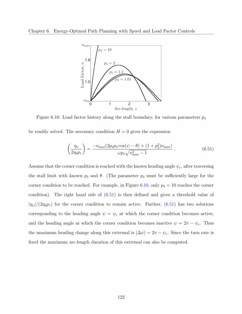
Chapter 6. Energy-Optimal Path Planning with Speed and Load Factor Controls
0 1 2 3
1.5
1.8
Figure 6.10: Load factor history along the stall boundary, for various parameters p3
be readily solved. The necessary condition H = 0 gives the expression
(ηψ
2η0p1
)=−nmax(2p2p3 cos(ψ − θ) + (1 + p2
2)nmax)
ωp2
√n2
max − 1. (6.51)
Assume that the corner condition is reached with the known heading angle ψc, after traversing
the stall limit with known p3 and θ. (The parameter p3 must be sufficiently large for the
corner condition to be reached. For example, in Figure 6.10, only p3 = 10 reaches the corner
condition). The right hand side of (6.51) is then defined and gives a threshold value of
|ηψ|/(2η0p1) for the corner condition to remain active. Further, (6.51) has two solutions
corresponding to the heading angle ψ = ψc at which the corner condition becomes active,
and the heading angle at which the corner condition becomes inactive ψ = 2π − ψc. Thus
the maximum heading change along this extremal is |∆ψ| = 2π − ψc. Since the turn rate is
fixed the maximum arc-length duration of this extremal can also be computed.
122

Chapter 6. Energy-Optimal Path Planning with Speed and Load Factor Controls
Maximum load factor constraint (only) active
For this case µ2 = 0 and n = nmax. Solving for the speed in (6.30) leads to
v =
[n2
max +ηψω
η0p1
√n2
max − 1
] 14
. (6.52)
Since ηψω = −ηψsgn(ηψ) = −|ηψ| < 0 then, the second term in (6.52) is negative, and it
follows that v <√nmax <
√nmax
p2< vc. However at n = nmax, the speed v < vc is not
admissible. Thus, this case can be ignored.
6.8 Path Synthesis
Further analysis may lead to additional optimality conditions and, possibly, an analytical
solution to the path synthesis problem of constructing the optimal extremal sequence that
satisfies the boundary conditions. However, in this work, the problem is solved numeri-
cally using the direct method employed by the Gauss Pseudospectral Optimization Software
(GPOPS) (Rao et al., 2010). The analysis of the extremal controls thus far gives insight re-
garding the structure of the optimal control problem that cannot be obtained by a numerical
solver alone. This analysis may be used to verify the numerical results, aid in the selection
of an appropriate initial guess, and to refine any solution that is obtained. (For example,
one could construct an analytical expression a posteriori for each extremal arc returned by
the solver.)
The software GPOPS requires the control variable constraints to be input as strict linear
inequalities. (Thus the constraint (6.18) is not acceptable.) Consider the change of variables
123
Chapter 6. Energy-Optimal Path Planning with Speed and Load Factor Controls
(v, n)→ (v, φ) satisfying:
v =
√1
p2 cosφ(1− v) + vmaxv , (6.53)
n =1
cosφ, (6.54)
where φ ∈ [−φmax, φmax] is the bank angle and v ∈ [0, 1] is the speed fraction at a given bank
angle (i.e. v = 0 is always along the stall boundary, while v = 1 is the maximum speed). With
these new variables, the control constraint set becomes Ω = (v, φ) ∈ [0, 1]× [−φmax, φmax]
which can be expressed as a series of linear inequality constraints. With these new variables,
the turn rate becomes
ψ′ =tanφ√
sec φ/p2(1− v) + vvmax
,
and the parameter ω is eliminated since the sense of the turn is given by the sign of the bank
angle φ. The cost functional becomes
J =
∫ s1
0
((√
sec φ/p2(1− v) + vvmax)2 +sec2 φ
(√
sec φ/p2(1− v) + v(s)vmax)2
)ds ,
whereas the state equations (6.13)-(6.14) remain unchanged. In Figures 6.11-6.13 results
are given for three final endpoints x1. The figures contain the resulting control history n(s)
and v(s), the pair (v, n) plotted over Ω, and the resulting optimal path to the goal for each
endpoint.
Referring to Figures 6.11(c)-6.13(c) the optimal control pairs (v, n) output by the solver
follow the extremal locus and stall boundary as expected. In each case the controls contain
a larger portion of the stall boundary and only in Figure 6.13(c) does the corner condition
become active. Examining Figures 6.11(a)-6.13(a) the controls along the extremal locus and
124
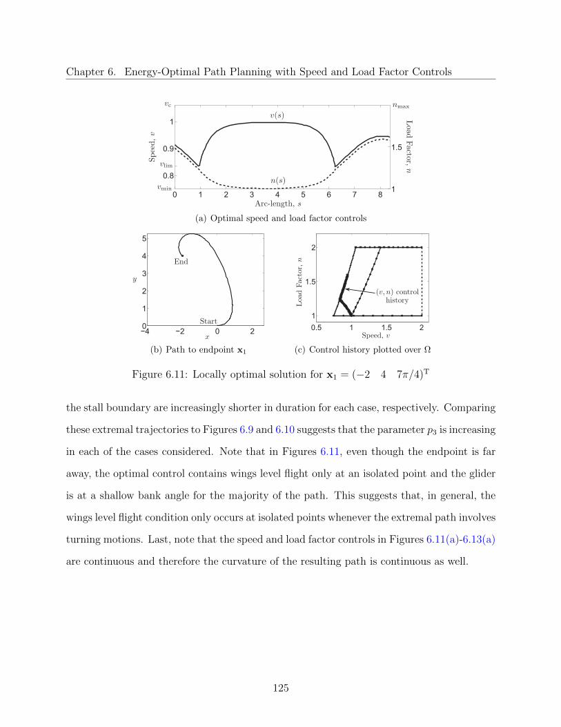
Chapter 6. Energy-Optimal Path Planning with Speed and Load Factor Controls
0 1 2 3 4 5 6 7 8
0.8
0.9
1
1
1.5
(a) Optimal speed and load factor controls
4 2 0 20
1
2
3
4
5
(b) Path to endpoint x1
0.5 1 1.5 2
1
1.5
2
(c) Control history plotted over Ω
Figure 6.11: Locally optimal solution for x1 = (−2 4 7π/4)T
the stall boundary are increasingly shorter in duration for each case, respectively. Comparing
these extremal trajectories to Figures 6.9 and 6.10 suggests that the parameter p3 is increasing
in each of the cases considered. Note that in Figures 6.11, even though the endpoint is far
away, the optimal control contains wings level flight only at an isolated point and the glider
is at a shallow bank angle for the majority of the path. This suggests that, in general, the
wings level flight condition only occurs at isolated points whenever the extremal path involves
turning motions. Last, note that the speed and load factor controls in Figures 6.11(a)-6.13(a)
are continuous and therefore the curvature of the resulting path is continuous as well.
125

Chapter 6. Energy-Optimal Path Planning with Speed and Load Factor Controls
0 1 2 3 4 5
0.8
0.9
1
1
1.5
(a) Optimal speed and load factor controls
0 0.5 1 1.5 2
1
0.5
0
0.5
(b) Path to endpoint x1
0.5 1 1.5 2
1
1.5
2
(c) Control history plotted over Ω
Figure 6.12: Locally optimal solution for x1 = (0 − 0.5 π)T
6.9 Conclusion
Here the minimum depth path planning problem of Chapter 5 is revisited and the shallow
bank angle constraint is relaxed. A physics-based turn rate and sink rate models is developed
in which the speed and load factor controls are coupled. It was found that the extremal
controls consist of: a) wings level flight at the minimum drag flight condition, b) a locus of
extremal controls on the interior of the admissible control set, c) a subset of controls along
the stall boundary, and d) the corner condition where the load factor is maximum and the
speed is minimum. The effect of the adjoint variables on the shape of the extremal arcs was
characterized in each case. The path synthesis problem was solved using the direct method
employed by the numerical solver GPOPS. The insight gained regarding the optimal controls,
and the proposed path synthesis approach, can be used to plan energy-optimal paths for a
126
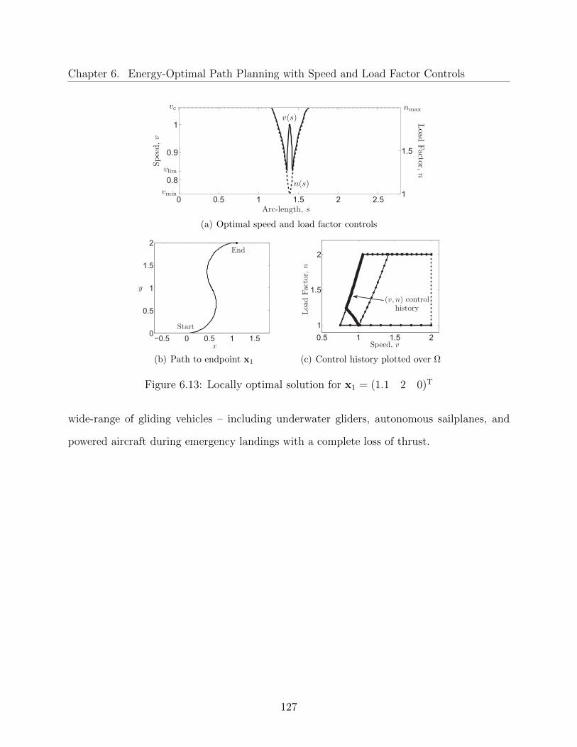
Chapter 6. Energy-Optimal Path Planning with Speed and Load Factor Controls
0 0.5 1 1.5 2 2.5
0.8
0.9
1
1
1.5
(a) Optimal speed and load factor controls
0.5 0 0.5 1 1.50
0.5
1
1.5
2
(b) Path to endpoint x1
0.5 1 1.5 2
1
1.5
2
(c) Control history plotted over Ω
Figure 6.13: Locally optimal solution for x1 = (1.1 2 0)T
wide-range of gliding vehicles – including underwater gliders, autonomous sailplanes, and
powered aircraft during emergency landings with a complete loss of thrust.
127

Chapter 7
Design and Testing of a Pneumatically
Propelled Underwater Glider
7.1 Introduction
The unique challenges associated with shallow waters, such as the presence of significant
currents, motivate developing new glider designs with improved capabilities. A few gliders
have been developed specifically for the coastal ocean. These include the shallow water
Slocum Battery (Creed et al., 2002) and more recently the Coastal Glider (Imlach and Mahr,
2012). The shallow water (200 m) Slocum Battery was designed with a single-stroke piston
style buoyancy engine. It employs a rudder to yaw (rather than rolling with a laterally moving
mass). This helps achieve a tight turning radius (of about 7 m) and improves maneuverability
(Davis et al., 2002). However the Slocum Battery only displaces 0.5 L of water with its
buoyancy engine, resulting in a top speed of 25 cm/s. Shallow water currents often exceed
this speed and can potentially dominate the dynamics of a slow moving glider. The Coastal
Glider has been in development for the past decade and is now being commercialized. It
128
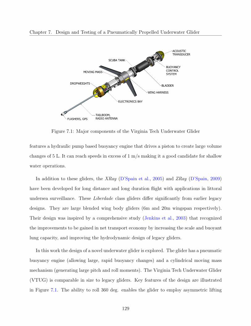
Chapter 7. Design and Testing of a Pneumatically Propelled Underwater Glider
Figure 7.1: Major components of the Virginia Tech Underwater Glider
features a hydraulic pump based buoyancy engine that drives a piston to create large volume
changes of 5 L. It can reach speeds in excess of 1 m/s making it a good candidate for shallow
water operations.
In addition to these gliders, the XRay (D’Spain et al., 2005) and ZRay (D’Spain, 2009)
have been developed for long distance and long duration flight with applications in littoral
undersea surveillance. These Liberdade class gliders differ significantly from earlier legacy
designs. They are large blended wing body gliders (6m and 20m wingspan respectively).
Their design was inspired by a comprehensive study (Jenkins et al., 2003) that recognized
the improvements to be gained in net transport economy by increasing the scale and buoyant
lung capacity, and improving the hydrodynamic design of legacy gliders.
In this work the design of a novel underwater glider is explored. The glider has a pneumatic
buoyancy engine (allowing large, rapid buoyancy changes) and a cylindrical moving mass
mechanism (generating large pitch and roll moments). The Virginia Tech Underwater Glider
(VTUG) is comparable in size to legacy gliders. Key features of the design are illustrated
in Figure 7.1. The ability to roll 360 deg. enables the glider to employ asymmetric lifting
129
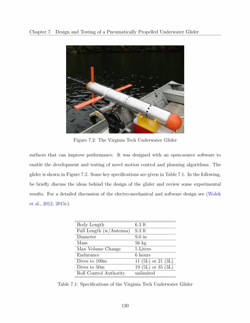
Chapter 7. Design and Testing of a Pneumatically Propelled Underwater Glider
Figure 7.2: The Virginia Tech Underwater Glider
surfaces that can improve performance. It was designed with an open-source software to
enable the development and testing of novel motion control and planning algorithms. The
glider is shown in Figure 7.2. Some key specifications are given in Table 7.1. In the following,
be briefly discuss the ideas behind the design of the glider and review some experimental
results. For a detailed discussion of the electro-mechanical and software design see (Wolek
et al., 2012, 2015c).
Body Length 6.3 ftFull Length (w/Antenna) 9.3 ftDiameter 9.0 inMass 56 kgMax Volume Change 5 LitersEndurance 6 hoursDives to 100m 11 (5L) or 21 (3L)Dives to 50m 19 (5L) or 35 (3L)Roll Control Authority unlimited
Table 7.1: Specifications of the Virginia Tech Underwater Glider
130
Chapter 7. Design and Testing of a Pneumatically Propelled Underwater Glider
7.2 Buoyancy Control
Underwater gliders control their depth rate by adjusting their net weight. This can be
achieved by either adjusting the weight of the vehicle (e.g. releasing drop weights, or flooding
ballast tanks) or by adjusting the buoyancy (e.g. inflating a bladder, or displacing water
in a flooded chamber using a piston). The mechanical device that adjusts buoyancy is
sometimes called the “buoyancy engine”, the “variable buoyancy device”, or the “buoyancy
control system”.
The total buoyancy B of a glider is the sum of the fixed buoyancy of the glider’s rigid
body BRB (for shallow waters hull compressibility may be neglected, this quantity can be
assumed ot be fixed) and the variable buoyancy generated by the buoyancy engine BBE. For
a glider with “dry weight” W = mg (where m is the glider’s mass and g is gravitational
acceleration), the net force on the glider is referred to as the net weight W = B −W . It is
convenient to express the net weight as a fraction of the dry weight using the buoyant lung
setting η such that W = ηW = (BRB + BBE −W ). For the glider to descend BRB < W is
required, and there is a value of BBE that gives neutral buoyancy (W = 0) corresponding
to η = 0. The buoyant lung capacity η is the maximum value of η. The buoyancy engine is
often designed such that η ∈ [−η, η] to produce equal forces in both ascents and descents.
Shallow Water Buoyancy Engine Requirements
Shallow waters are often characterized by strong currents. Legacy gliders operate at hori-
zontal speed of about 0.6 kts and, at such low speeds, typical currents in the coastal ocean
can dominate the glider’s dynamics. This gap in speed motivates the design of faster gliders
with larger buoyant lung capacities. Gliders are most efficient while in a steady equilibrium
glide. Thus it is desirable to minimize the time it takes to transition from a dive to an
131

Chapter 7. Design and Testing of a Pneumatically Propelled Underwater Glider
Requirement ValueBuoyant Lung Capacity ± 5 % (± 2,500 cc assuming a 50 kg glider)Buoyancy Transfer Time ≤ 10 sec. (167 cc/s)Max. Operational Depth 100 mEndurance 6 hoursWeight ≤ 30 lbs (≈ 25% of vehicle dry weight)Size ≤ 20 in. length (≈ 25% of vehicle length)
Table 7.2: Buoyancy engine design requirements
ascent, and vice versa. This is particularly important in shallow waters where there may
not be sufficient depth to establish a steady glide. Let the time that it takes the buoyancy
engine to change from −η to η be the buoyancy transfer time. (Note that the speed of the
moving mass actuator will also determine the time it takes to achieve a steady glide.)
The endurance of the vehicle was required to be long enough for a full day of field testing;
about a 6 hour deployment. The maximum operating depth was limited to 100 m. The
buoyancy engine was required to have a large buoyant lung capacity (an order of magnitude
larger than previous gliders) and a small buoyancy transfer time (less than 10 seconds).
These requirements are summarized in Table 7.2.
Selecting the Buoyancy Control Mechanism
There have been many mechanisms proposed for the purpose of buoyancy control. Traditional
buoyancy control mechanisms include piston-cylinder designs (Creed et al., 2002), hydraulic
pump-powered bladders (Sherman et al., 2001; Eriksen et al., 2001) and the use of ballast
tanks (as employed by manned submarines). Thermally driven phase-change buoyancy en-
gines that harvest energy have been proven (Webb et al., 2001). Chemical reactions with
surrounding seawater to produce gases for buoyancy control have been proposed (Cameron,
2005; Borchsenius and Pinder, 2010). Using shape memory alloys to change the hull dis-
132

Chapter 7. Design and Testing of a Pneumatically Propelled Underwater Glider
placement for buoyancy control has also been investigated (Mide Technology Corporation,
2015). A detailed discussion of the working principle behind each of these technologies is
beyond the scope of this work. In the following, the main reasons for choosing a pneumatic
buoyancy engine are briefly discussed.
A piston-cylinder buoyancy engine designed with a 8 inch diameter face (about the diam-
eter of a typical glider hull) would require over 8,000 lbs of force to actuate at 100 m depth.
Pretensioning the piston or reducing the piston face area (at the cost of a larger stroke)
would reduce this force requirement. However, the power requirements to achieve the de-
sired transfer time remained prohibitive. Commercially available linear actuators (leadscrew
and motor or hydraulic types) designed for industrial applications were determined to be too
large and heavy to be viable options.
Oil-bladder and pump designs used by legacy gliders are efficient at high pressures and
large depths. To meet the buoyancy engine requirements, a fast and large displacement
pump would be required. A common challenge associated with pump based buoyancy engine
designs is the presence of air bubbles in the working fluid. Such air bubbles may be difficult
to remove and under some conditions may result in a reduction or loss of pumping power.
A preliminary study of this concept concluded that commercially available pumps would
not meet the required specifications with a reasonable weight and volume or would require
engineering design and fabrication procedures that would far exceed the allocated budget.
A pneumatic buoyancy engine was ultimately chosen for the VTUG. Energy stored in the
form of compressed air, housed in a diving cylinder (scuba tank), can be used directly to
inflate an elastomeric bladder for buoyancy. This approach does not have the efficiency losses
associated with converting electrical to mechanical energy, as in battery powered designs.
The pressure differential between the ambient water at 100 m and a scuba tank is over 3,000
psi. (In theory, the tank’s pressure differential allows inflating the bladder at depths up to 2
133

Chapter 7. Design and Testing of a Pneumatically Propelled Underwater Glider
Model Faber FX23DVMax Pressure 3,442 psiTank Size 23 std. cu. ftInternal Volume 183 cu. in.Length 19.5 in.Diameter 3.9 in.Empty Weight 8.6 lbs
Table 7.3: Scuba tank specifications
km.) A rapid inflation of a large volume can be achieved by simply opening a valve. In this
design, the buoyancy engine is an open system and air must be exhausted to the hydrosphere
to reduce the buoyancy of the bladder once it is inflated. The endurance of the vehicle is
limited by the capacity of the tank.
Design of a Pneumatic Buoyancy Engine
Conceptual Design
Scuba tanks with compressed air are an ideal choice for a pneumatic buoyancy engine because
they are designed to operate in water, are safe, and can be readily re-filled at local dive shops.
For the VTUG, a “pony” sized tank was found to have sufficient air capacity for the mission
endurance required. (A pony tank is a smaller scuba tank typically used by divers as an
extra air supply in emergency situations.) A steel tank was selected because of its higher air
capacity to weight ratio relative to aluminum tanks. The specifications of the tank are given
in Table 7.3.
To assess the performance of the pneumatic buoyancy engine concept, it is assumed that
134

Chapter 7. Design and Testing of a Pneumatically Propelled Underwater Glider
the air behaves according to the ideal gas law:
p V– = nRT (7.1)
where
p = pressure (Pa)
V– = volume (m3)
n = amount of gas (moles)
R = universal gas constant
(8.314
J ·mole
K
).
T = temperature (K)
The initial amount of gas ntank inside the tank at room temperature can be computed from
(7.1) using the parameters in Table 7.3. In this case, ntank ≈ 31.1 moles. For a given buoyant
lung setting, the volume of water displaced by the buoyancy engine is V– η = ηW/ρH2Og where
and ρH2O is the density of water. At a given depth z (and corresponding ambient pressure
pamb) the ideal gas law (7.1) can be used to compute the amount of air ncycle required
to displace the volume V– η under ideal conditions. (This neglects the additional pressure
required to stretch the bladder and other losses.) The ideal number of available dives for
a given scuba tank is then N = ntank/ncycle. Contours of fixed N are shown in Figure 7.3,
for various bladder displacements and depths, given the scuba tank parameters in Table 7.3.
At the most extreme design point (5 L displacement, 100 m depth) thus an endurance of 13
dives is expected, while at shallower depths many more dives can be expected. (Replacing
the scuba tank in the field can further extend endurance.)
In the previous discussion, it was assumed the bladder was inflated to the same volume at
135

Chapter 7. Design and Testing of a Pneumatically Propelled Underwater Glider
BladdervDisplacement,vL
Dep
th,vm
2.5 3 3.5 4 4.5 5
30
40
50
60
70
80
90
100No.vDives
20
30
40
50
60
70
Figure 7.3: Number of dives
the same depth with each dive. However this will generally result in different ascent/descent
profiles with each dive, due to two factors: a) the vehicle becomes lighter as the tank is de-
pleted, and b) as the ambient pressure changes with depth, the bladder will expand/compress
unless the pressure is actively regulated (with feedback control). In the following these two
effects are discussed.
The weight of air in the tank at full pressure (3,442 psi) is about 2 lbs. Assume that
the vehicle is trimmed to be neutrally buoyant with a tank full and a bladder displacement
of 2.5 L (at η = 0). Then if every ascent corresponds to a bladder displacement of 5 L
(fully inflated, η = η) and every descent to a displacement of 0 L (fully deflated, η = −η),
the change in net weight as the tank becomes depleted is given by Figure 7.4. As the tank
becomes lighter, the range of attainable net weights shifts towards higher buoyancy and the
trim point will change significantly during the course of a single deployment.
The second effect results from the changes in ambient pressure around the elastomeric
bladder. Let pblad account for the pressure resulting from the elastic forces in a stretched
136

Chapter 7. Design and Testing of a Pneumatically Propelled Underwater Glider
0 0.5 1 1.5
−4
−2
0
2
4
6
Tank Air Weight (lbs)
Net
Wei
ght (
lbs)
5 L2.5 L0 L
Figure 7.4: Net weight with bladder volume for various scuba tank weights
bladder. The bladder reaches an equilibrium volume when the ambient pressure pamb and
elastic bladder pressure pblad is balanced by the internal bladder pressure pint:
pamb + pblad − pint = 0 . (7.2)
The ambient pressure is given by the hydrostatic equation
pamb = patm + ρH2Ogz , (7.3)
where patm is the atmospheric pressure. Assume that the elastic pressure pblad = pblad(V– )
depends only on the volume of the stretched bladder. The internal bladder pressure is given
by the ideal gas law
pint =nRT
V–. (7.4)
137
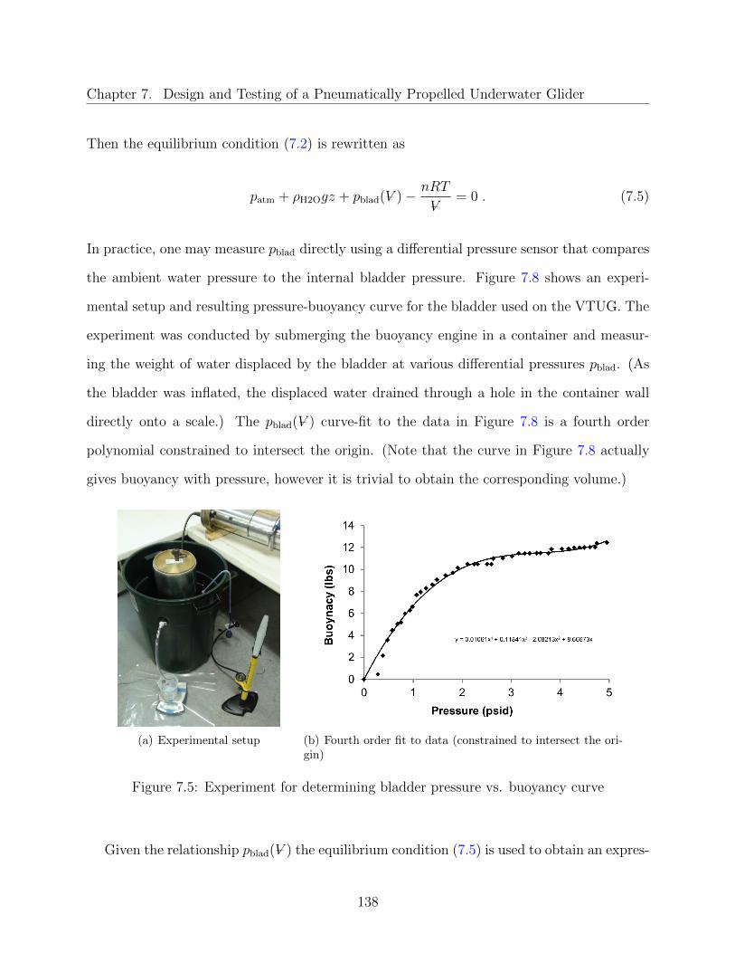
Chapter 7. Design and Testing of a Pneumatically Propelled Underwater Glider
Then the equilibrium condition (7.2) is rewritten as
patm + ρH2Ogz + pblad(V– )− nRT
V–= 0 . (7.5)
In practice, one may measure pblad directly using a differential pressure sensor that compares
the ambient water pressure to the internal bladder pressure. Figure 7.8 shows an experi-
mental setup and resulting pressure-buoyancy curve for the bladder used on the VTUG. The
experiment was conducted by submerging the buoyancy engine in a container and measur-
ing the weight of water displaced by the bladder at various differential pressures pblad. (As
the bladder was inflated, the displaced water drained through a hole in the container wall
directly onto a scale.) The pblad(V– ) curve-fit to the data in Figure 7.8 is a fourth order
polynomial constrained to intersect the origin. (Note that the curve in Figure 7.8 actually
gives buoyancy with pressure, however it is trivial to obtain the corresponding volume.)
(a) Experimental setup (b) Fourth order fit to data (constrained to intersect the ori-gin)
Figure 7.5: Experiment for determining bladder pressure vs. buoyancy curve
Given the relationship pblad(V– ) the equilibrium condition (7.5) is used to obtain an expres-
138
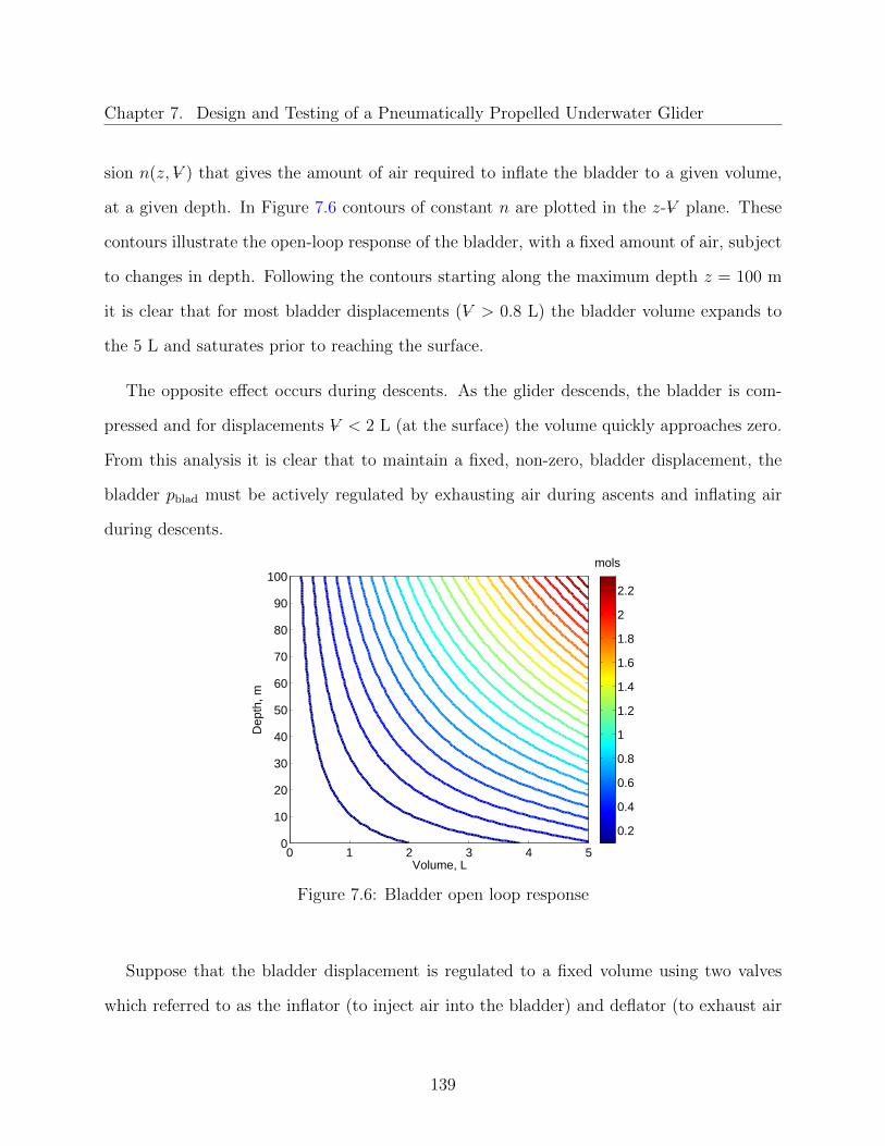
Chapter 7. Design and Testing of a Pneumatically Propelled Underwater Glider
sion n(z, V– ) that gives the amount of air required to inflate the bladder to a given volume,
at a given depth. In Figure 7.6 contours of constant n are plotted in the z-V– plane. These
contours illustrate the open-loop response of the bladder, with a fixed amount of air, subject
to changes in depth. Following the contours starting along the maximum depth z = 100 m
it is clear that for most bladder displacements (V– > 0.8 L) the bladder volume expands to
the 5 L and saturates prior to reaching the surface.
The opposite effect occurs during descents. As the glider descends, the bladder is com-
pressed and for displacements V– < 2 L (at the surface) the volume quickly approaches zero.
From this analysis it is clear that to maintain a fixed, non-zero, bladder displacement, the
bladder pblad must be actively regulated by exhausting air during ascents and inflating air
during descents.
Volume, L
Dep
th, m
0 1 2 3 4 50
10
20
30
40
50
60
70
80
90
100mols
0.2
0.4
0.6
0.8
1
1.2
1.4
1.6
1.8
2
2.2
Figure 7.6: Bladder open loop response
Suppose that the bladder displacement is regulated to a fixed volume using two valves
which referred to as the inflator (to inject air into the bladder) and deflator (to exhaust air
139

Chapter 7. Design and Testing of a Pneumatically Propelled Underwater Glider
to the hydrosphere). Holding V– fixed, and differentiating (7.5)
ρH2Ogz =nRT
V–. (7.6)
From (7.6) the air exchange rate n required for a given depth rate z may be determined.
The range of expected depth rates will depend on the buoyant lung setting and drag of the
glider. A conservative estimate for the maximum depth rate can be obtained by equating
the net weight to the drag force. This gives the terminal velocity
zmax =
√2ηW
ρH2OSCD, (7.7)
where S is the surface area and CD is the drag coefficient. Depending on the orientation
of the glider the drag coefficient may vary. (The worst case orientation is assumed where
the glider is pointed downwards and is most streamlined. In this case, the surface area can
be taken as the hull cross-sectional area.) Equations (7.7) and (7.6) give a conservative
estimate of the required amount of air to be exhausted/inflated by the valves to maintain
a fixed bladder volume. This estimate is shown in Figure 7.7 for several drag coefficients,
where each curve is generated by computing zmax and n, from (7.7) and (7.6), for η varying
from −η to η. It is interesting to note that there is a maximum air exchange rate during
descents. At η = 0 the bladder displacement is 2.5 L corresponding to neutral buoyancy and
thus zmax = 0 and n = 0. As η decreases to −η, the bladder becomes completely deflated
and there is no need to exchange air, and again n = 0. In-between these two conditions the
maximum required inflation rate occurs. On the other hand, the air exchange rate magnitude
is monotonically increasing with η during ascents. The most demanding air exchange rate
occurs when the drag coefficient is low during highest speed ascents. (A large amount of air
must be continuously exhausted to maintain a fixed bladder volume during this condition.)
140

Chapter 7. Design and Testing of a Pneumatically Propelled Underwater Glider
−4 −3 −2 −1 0 1 2 3 4−0.08
−0.07
−0.06
−0.05
−0.04
−0.03
−0.02
−0.01
0
0.01
0.02
Airp
Exc
hang
epR
ate,
pmol
/s
DepthpRate,pm/s
CD
=p0.25
CD
=p0.1
CD
=p1
Figure 7.7: Inflator and deflator requirements
Having established the required air exchange rates it remains to select actuators (valves
and tubing) to meet these requirements. Generally, vendors of flow control valves provide
flow coefficients (Cv) or volumetric flow rate curves for various differential pressures. The
flow coefficient for gas flow (Swagelok Company, 2007) is given by
q = NCvp1
(1− 2∆p
3p1
)√∆p
p1T1
, (7.8)
141
Chapter 7. Design and Testing of a Pneumatically Propelled Underwater Glider
where
q = volumetric flow rate (std. ft3/min)
p1 = inlet pressure (psia)
p2 = outlet pressure (psia)
∆p = p1 − p2, differential pressure (psid)
T1 = absolute temperature (R)
N = 22.67 (constant depending on unit choice).
In Figure 7.8(a), the deflator flow coefficient Cv is calculated from (7.8) for a range of bladder
displacements and depths. For a given bladder displacement and depth, the corresponding
maximum depth rate and air exchange rate are calculated using (7.7) and (7.6), assuming
CD = 0.1 (the worst case). Recall that mair = nMair relates an amount of air n to the mass
of the air mair where where Mair is the molecular weight of air. Then the volumetric flow
rate is
q =mair
ρair
=nMair
ρair
.
For sizing the deflator, ∆p = pblad(V– ), and the hydrostatic equation (7.3) can be used to
compute p2 = pamb. Then p1 = pamb + ∆p. From Figure 7.8(a), the deflator requirements
(to maintain a fixed bladder volume) increase with depth and bladder displacement.
A similar analysis can be used to size the inflator. The flow into the bladder is driven by
the large pressure differential between the scuba tank and the internal bladder pressure. Thus
the effects of changes in depth can be ignored. From Figure 7.8(b), the Cv is significantly
lower than that of the deflator. Further, there is a bladder displacement that maximizes the
required Cv, and this is related to the maximum air exchange rate n seen in Figure 7.7.
142
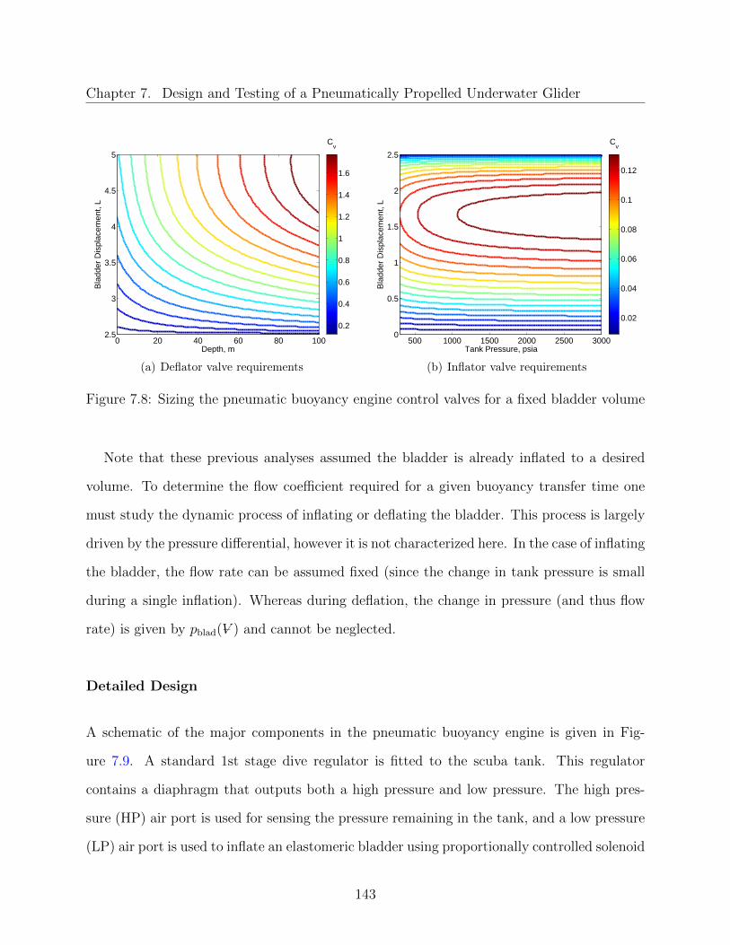
Chapter 7. Design and Testing of a Pneumatically Propelled Underwater Glider
Depth, m
Bla
dder
Dis
plac
emen
t, L
0 20 40 60 80 1002.5
3
3.5
4
4.5
5
Cv
0.2
0.4
0.6
0.8
1
1.2
1.4
1.6
(a) Deflator valve requirements
Tank8Pressure,8psia
Bla
dder
8Dis
plac
emen
t,8L
500 1000 1500 2000 2500 30000
0.5
1
1.5
2
2.5
Cv
0.02
0.04
0.06
0.08
0.1
0.12
(b) Inflator valve requirements
Figure 7.8: Sizing the pneumatic buoyancy engine control valves for a fixed bladder volume
Note that these previous analyses assumed the bladder is already inflated to a desired
volume. To determine the flow coefficient required for a given buoyancy transfer time one
must study the dynamic process of inflating or deflating the bladder. This process is largely
driven by the pressure differential, however it is not characterized here. In the case of inflating
the bladder, the flow rate can be assumed fixed (since the change in tank pressure is small
during a single inflation). Whereas during deflation, the change in pressure (and thus flow
rate) is given by pblad(V– ) and cannot be neglected.
Detailed Design
A schematic of the major components in the pneumatic buoyancy engine is given in Fig-
ure 7.9. A standard 1st stage dive regulator is fitted to the scuba tank. This regulator
contains a diaphragm that outputs both a high pressure and low pressure. The high pres-
sure (HP) air port is used for sensing the pressure remaining in the tank, and a low pressure
(LP) air port is used to inflate an elastomeric bladder using proportionally controlled solenoid
143
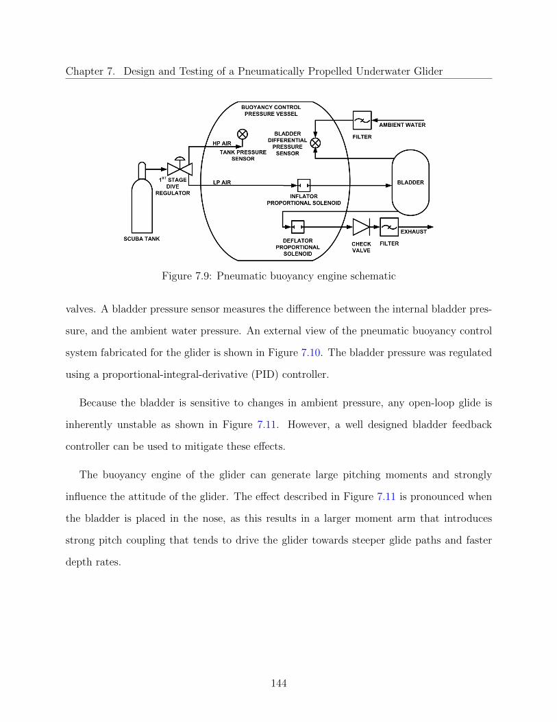
Chapter 7. Design and Testing of a Pneumatically Propelled Underwater Glider
Figure 7.9: Pneumatic buoyancy engine schematic
valves. A bladder pressure sensor measures the difference between the internal bladder pres-
sure, and the ambient water pressure. An external view of the pneumatic buoyancy control
system fabricated for the glider is shown in Figure 7.10. The bladder pressure was regulated
using a proportional-integral-derivative (PID) controller.
Because the bladder is sensitive to changes in ambient pressure, any open-loop glide is
inherently unstable as shown in Figure 7.11. However, a well designed bladder feedback
controller can be used to mitigate these effects.
The buoyancy engine of the glider can generate large pitching moments and strongly
influence the attitude of the glider. The effect described in Figure 7.11 is pronounced when
the bladder is placed in the nose, as this results in a larger moment arm that introduces
strong pitch coupling that tends to drive the glider towards steeper glide paths and faster
depth rates.
144
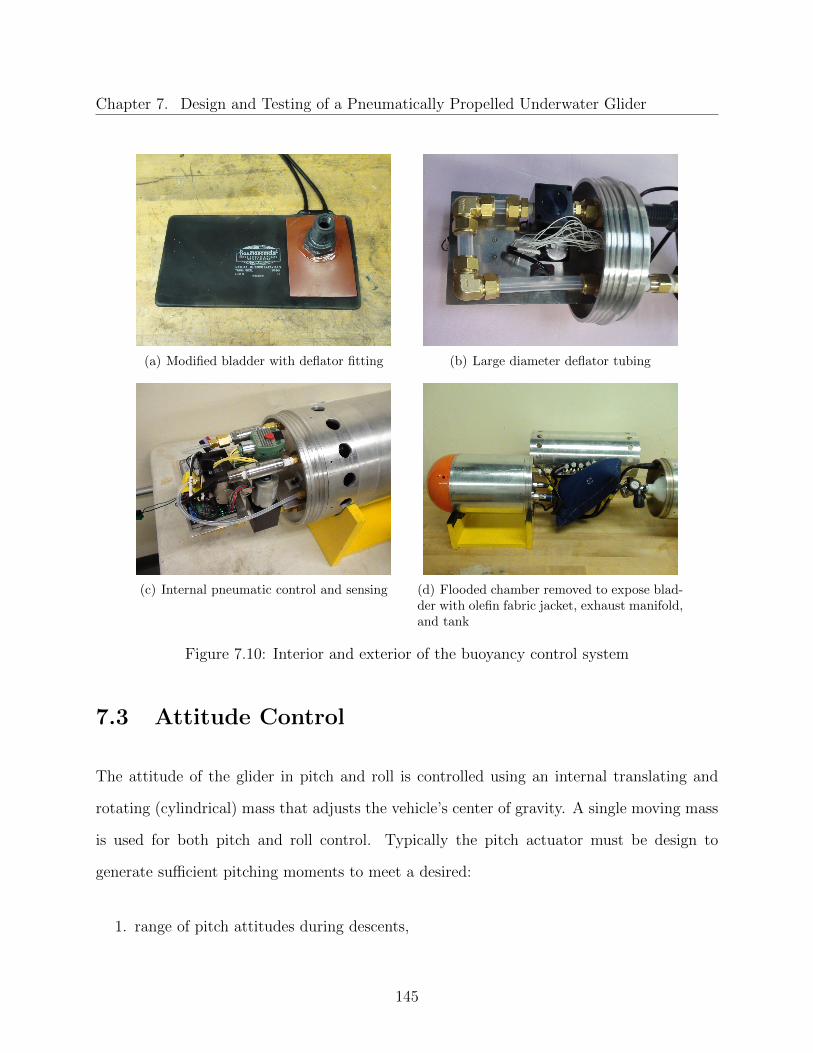
Chapter 7. Design and Testing of a Pneumatically Propelled Underwater Glider
(a) Modified bladder with deflator fitting (b) Large diameter deflator tubing
(c) Internal pneumatic control and sensing (d) Flooded chamber removed to expose blad-der with olefin fabric jacket, exhaust manifold,and tank
Figure 7.10: Interior and exterior of the buoyancy control system
7.3 Attitude Control
The attitude of the glider in pitch and roll is controlled using an internal translating and
rotating (cylindrical) mass that adjusts the vehicle’s center of gravity. A single moving mass
is used for both pitch and roll control. Typically the pitch actuator must be design to
generate sufficient pitching moments to meet a desired:
1. range of pitch attitudes during descents,
145

Chapter 7. Design and Testing of a Pneumatically Propelled Underwater Glider
During an open-loop descent:1) Depth and ambient pressure increase 2) The bladder is compressed and buoyancy is reduced3) Depth rate increases
depthrate vector
Figure 7.11: Unstable (open-loop) bladder pressure and depth rate coupling
2. range of pitch attitudes during ascents,
3. pitch attitude during surface communication.
A free body diagram of the forces acting on a glider in a steady, equilibrium glide is shown
in Figure 7.12. (For the purpose of determining a range of pitch attitudes, the lift and drag
forces are neglected here.) It is assumed that all of the forces act along the vehicle centerline,
with the exception of the moving mass weight WMM (which is assumed to act a distance zMM
below the centerline). The attainable pitch angles will change with the buoyancy generated
by the buoyancy engine BBE, and the weight of the tank WT. The remaining weight of the
rigid body (excluding WMM and WT) is denoted WRB. Similarly, the buoyancy of the rigid
body (excluding BBE) is denoted BRB. The longitudinal location through which each force
acts is measured from the back of the vehicle (indicated by l in Figure 7.12). Then the
conditions for equilibrium are:
ΣFz : WMM +WT +WRB −BRB +BBE = 0 (7.9)
ΣM : (lMM + zMM tan θ)WMM + (lTWT + lRBWRB − lRBBRB + lBEBBE) = 0 (7.10)
146

Chapter 7. Design and Testing of a Pneumatically Propelled Underwater Glider
where θ is the pitch angle.
Figure 7.12: Forces acting on the glider in an steady equilibrium pitch attitude
If the moving mass can travel from lMM ∈ [lMM,min, lMM,max], then using (7.9) and (7.10) the
range of possible pitch attitudes can be computed for a given bladder buoyancy and tank
weight. The center of gravity (CG) and center of buoyancy (CB) positions in the vertical
plane are given by:
CGx =lMMWMM + lTWT + lRBWRB
WMM +WT +WRB
(7.11)
CGz =zMMWMM
WMM +WT +WRB
(7.12)
CBx =lRBBRB + lBEWBE
BBE +BRB
(7.13)
CBz = 0 . (7.14)
Note that when the vehicle is on the surface, the problem of determining the CB is much
more complex. One must account for the discontinuity in the fluid density. (The buoyancy
of the portions of the glider exposed to the air is negligible.) On the VTUG, the tank was
placed close to CB to reduce the effect on the pitch trim of the vehicle.
The moving mass is actuated with a motor driven lead-screw in translation and a gearing
mechanism in rotation. Using polymer plain bearings, the linear portion of the mass slides
147
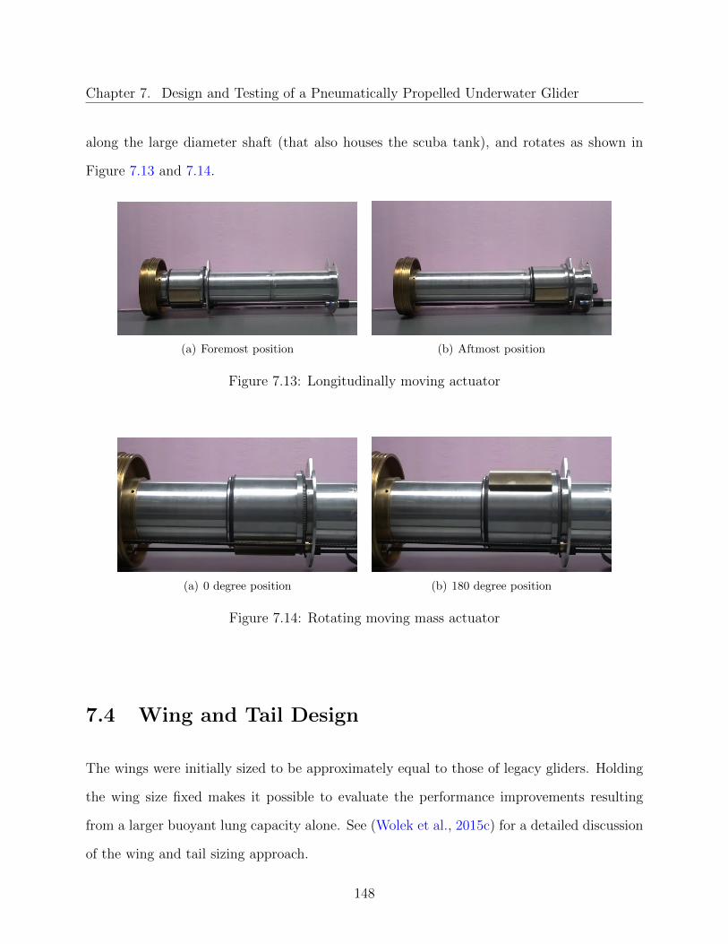
Chapter 7. Design and Testing of a Pneumatically Propelled Underwater Glider
along the large diameter shaft (that also houses the scuba tank), and rotates as shown in
Figure 7.13 and 7.14.
(a) Foremost position (b) Aftmost position
Figure 7.13: Longitudinally moving actuator
(a) 0 degree position (b) 180 degree position
Figure 7.14: Rotating moving mass actuator
7.4 Wing and Tail Design
The wings were initially sized to be approximately equal to those of legacy gliders. Holding
the wing size fixed makes it possible to evaluate the performance improvements resulting
from a larger buoyant lung capacity alone. See (Wolek et al., 2015c) for a detailed discussion
of the wing and tail sizing approach.
148

Chapter 7. Design and Testing of a Pneumatically Propelled Underwater Glider
A wing harness was designed to hold the wing in a number of asymmetric geometries,
including various dihedral angles (affecting roll stability), wing incidence angles (affecting
drag) and at various longitudinal positions (affecting pitch stability) (see Figure 7.15). How-
ever, to change other wing parameters such as wing camber, twist, or taper ratio, new wings
must be fabricated.
(a) Nominal wing incidence angle, 0 (b) Maximum wing incidence angle, 30
(c) Foremost wing position (d) Aftmost wing position
(e) Nominal dihedral angle, 0 (f) Maximum dihedral angle, 20
Figure 7.15: Range of asymmetric geometries provided by the wing harness
To estimate the performance improvements expected from a larger buoyant lung capac-
149
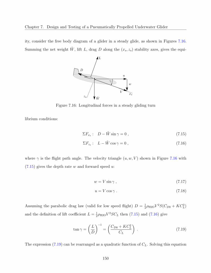
Chapter 7. Design and Testing of a Pneumatically Propelled Underwater Glider
ity, consider the free body diagram of a glider in a steady glide, as shown in Figures 7.16.
Summing the net weight W , lift L, drag D along the (xs, zs) stability axes, gives the equi-
Figure 7.16: Longitudinal forces in a steady gliding turn
librium conditions:
ΣFxs : D − W sin γ = 0 , (7.15)
ΣFzs : L− W cos γ = 0 , (7.16)
where γ is the flight path angle. The velocity triangle (u,w, V ) shown in Figure 7.16 with
(7.15) gives the depth rate w and forward speed u:
w = V sin γ , (7.17)
u = V cos γ . (7.18)
Assuming the parabolic drag law (valid for low speed flight) D = 12ρH2OV
2S(CD0 + KC2L)
and the definition of lift coefficient L = 12ρH2OV
2SCL then (7.15) and (7.16) give
tan γ =
(L
D
)−1
=
(CD0 +KC2
L
CL
). (7.19)
The expression (7.19) can be rearranged as a quadratic function of CL. Solving this equation
150
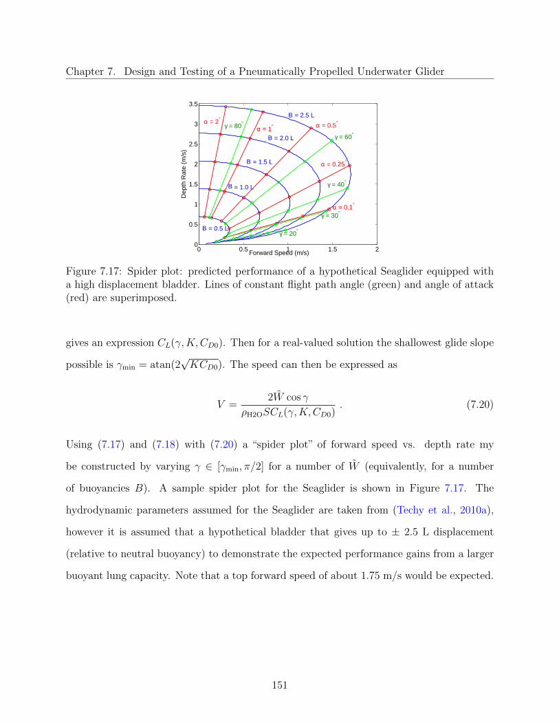
Chapter 7. Design and Testing of a Pneumatically Propelled Underwater Glider
0 0.5 1 1.5 20
0.5
1
1.5
2
2.5
3
3.5
Forward6Speed6(m/s)
Dep
th6R
ate6
(m/s
)
V6=62.56L
V6=62.06L
V6=60.56L
V6=61.06L
V6=61.56L
α =61° α =60.5°
α =60.25°
γ =630°α =60.1°
γ =620°
α =62°
γ =640°
γ =660°
γ =680°
B
B
B
B
B
Figure 7.17: Spider plot: predicted performance of a hypothetical Seaglider equipped witha high displacement bladder. Lines of constant flight path angle (green) and angle of attack(red) are superimposed.
gives an expression CL(γ,K,CD0). Then for a real-valued solution the shallowest glide slope
possible is γmin = atan(2√KCD0). The speed can then be expressed as
V =2W cos γ
ρH2OSCL(γ,K,CD0). (7.20)
Using (7.17) and (7.18) with (7.20) a “spider plot” of forward speed vs. depth rate my
be constructed by varying γ ∈ [γmin, π/2] for a number of W (equivalently, for a number
of buoyancies B). A sample spider plot for the Seaglider is shown in Figure 7.17. The
hydrodynamic parameters assumed for the Seaglider are taken from (Techy et al., 2010a),
however it is assumed that a hypothetical bladder that gives up to ± 2.5 L displacement
(relative to neutral buoyancy) to demonstrate the expected performance gains from a larger
buoyant lung capacity. Note that a top forward speed of about 1.75 m/s would be expected.
151
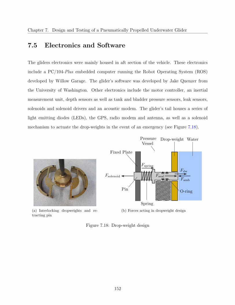
Chapter 7. Design and Testing of a Pneumatically Propelled Underwater Glider
7.5 Electronics and Software
The gliders electronics were mainly housed in aft section of the vehicle. These electronics
include a PC/104-Plus embedded computer running the Robot Operating System (ROS)
developed by Willow Garage. The glider’s software was developed by Jake Quenzer from
the University of Washington. Other electronics include the motor controller, an inertial
measurement unit, depth sensors as well as tank and bladder pressure sensors, leak sensors,
solenoids and solenoid drivers and an acoustic modem. The glider’s tail houses a series of
light emitting diodes (LEDs), the GPS, radio modem and antenna, as well as a solenoid
mechanism to actuate the drop-weights in the event of an emergency (see Figure 7.18).
(a) Interlocking dropweights and re-tracting pin
(b) Forces acting in dropweight design
Figure 7.18: Drop-weight design
152

Chapter 7. Design and Testing of a Pneumatically Propelled Underwater Glider
7.6 Acoustic Positioning and Communication
The VTUG employs an acoustic positioning and communication system developed by Tejaswi
Gode. The following discussion is adapted from (Gode, 2015).
Acoustics communication is relatively bandwidth limited and can be challenging in certain
environments, especially where the speed of sound profile is not properly characterized or ac-
counted for. Further challenges arise from multi-path, propagation delays and Doppler-shifts
(when applicable). Nonetheless, this method of underwater communication remains the most
effective and widely used. In the absence of an acoustic positioning system, underwater ve-
hicles typically employ the dead reckoning technique. Dead reckoning uses an initial position
(e.g. obtained using GPS) and measurements from an inertial navigation system to estimate
the position of the vehicle. (Often the inertial navigation system consists of accelerometers,
gyroscopes and a magnetometer.) Sources of error associated with the technique include
the inherent sensor error and exogenous disturbances (Gode, 2015; Bingham, 2009; Kapaldo,
2005). More advanced sensors, such as doppler velocity logs or gyro-compasses may improve
a dead reckoned estimate, however they ultimately suffer from the same sources of error.
Acoustic ranging systems provide independent position estimates that do not degrade
with time (i.e. they do not suffer from error drift). They require deploying a number
of transducers, and accompany acoustic modems, at known locations in the vicinity of an
underwater vehicle. The distance between these transducers is called the baseline. Depending
on the geometry of the transducer network they may be referred to as short baseline (SBL),
ultra short baseline (USBL), and long baseline (LBL) positioning systems (see Figure 7.19).
An acoustic ranging system works by successively sending an acoustic pulse (a “ping”)
to each transducer in the network. Upon receiving a response, the travel time of sound
between two transducers can be computed. Assuming some acoustic properties of the water
153

Chapter 7. Design and Testing of a Pneumatically Propelled Underwater Glider
GPS
Baseline ≈ <10cm
(a) A USBL is typically < 10cm
GPS
Baseline ≈ 20 – 50m
(b) A SBL is typically 20− 50m
GPS
Baseline ≈ 100m – 10km
(c) A LBL is typically 100m −10km
Figure 7.19: Types of acoustic baseline geometries. Used with permission (Gode, 2015).
(namely the speed of sound profile), the distance between transducers may be estimated.
These measurements can then be used to estimate the unknown position of the underwater
vehicle. The estimation algorithms may either be static or dynamic. Static estimates are
based purely on the geometry of the system (e.g. the intersection point of a series of spheres is
estimated using a least-squares solution). Dynamic estimates (e.g. obtained using a Kalman
filter) incorporate a dynamic model of the vehicle and additional sensor measurements.
While much of the previous discussion was limited to discussing acoustic positioning, the
same acoustic network can be used to communicate with the vehicle while it is underway.
However, because this communication is bandwidth-limited, generally only the most critical
information is communicated in this way (e.g. occasional updates on vehicle health and
status, or high-level commands from human operators).
As opposed to the fixed acoustic beacons typical of an LBL system (as in Figure 7.19(c)),
the VTUG uses a mobile network in which each beacon is deployed on an anchored, floating,
GPS-equipped raft as shown in Figure 7.20.
154

Chapter 7. Design and Testing of a Pneumatically Propelled Underwater Glider
Figure 7.20: Beacon deployed on a raft. Used with permission (Gode, 2015).
7.7 Testing
Buoyancy Engine Feasibility
To determine the feasibility of the pneumatic buoyancy engine concept, and to test a number
of components selected, a prototype buoyancy control system was fabricated. The prototype
consisted of a large scuba tank, a pressure vessel housing on/off type solenoid valves and
bladder pressure and depth sensors, as well as flooded chamber that housed the elastomeric
bladder, see Figure 7.21. The rig was trimmed to remain vertical.
Tests of this system were conducted in January 2012 at War Memorial Swimming Pool
on Virginia Tech’s campus. In these experiments a bang-bang controller was designed to
maintain a desired depth within some deadzone. It was found that the pneumatic system
was able to reliably make the rig ascend and descend. However, it was found that finely
155

Chapter 7. Design and Testing of a Pneumatically Propelled Underwater Glider
Figure 7.21: Feasibility test of the pneumatic buoyancy engine
regulating the bladder pressure was made difficult due to the coarse pressure changes provided
by the on/off type solenoids. The influence of the inflator on the bladder pressure was
disproportionately greater than that of the deflator. This test motivated revisiting the valve
sizing and selection approach. As a result of further analysis, new proportionally controlled
valves were selected. The diameter of the tubing and valve orifice in the deflation assembly
was increased to improve the deflation rate.
Depth Rating Validation
In August 2012, the glider was tested in Lake Washington by deploying it with a tether to a
depth of 25 m (see Figure 7.22). The purpose of the test was to verify the bladder is capable
of inflating at this depth, and also to confirm the vehicle is properly waterproofed.
Sawtooth Glides in Pool
A series of pool tests culminated with the glider performing a sawtooth glides across the pool
in March 2013 (as shown in Figure 7.23(a)). The glider employed a modified bladder that
156

Chapter 7. Design and Testing of a Pneumatically Propelled Underwater Glider
(a) Glider in tank for trimming at theUniversity of Washington
(b) Glider being launched from a sail-boat
(c) Tethered glider in Lake Washington
Figure 7.22: Lake Washington Depth Rating Test
used a fabric covering to restrict expansion beyond some volume and allow higher pressures
(up to 5 psi). This resulted in faster deflation rates and made the bladder less susceptible
to small changes in ambient pressure (as might occur from the vehicle pitching or changing
depth). The data from this test is given in Figure 7.23(b). The glider was able to traverse
the width of the diving well (≈ 20 m) in about two minutes. It is important to note that
the pool is much too shallow for the glider to establish a steady glide and the sawtooth here
consists of inefficient transient motions. The bladder pressure oscillated near the surface and
further gain tuning was required. The target depth of the glider during the sawtooth (black
dashed line, top right subplot in Figure 7.23(b)) was overshot by about 1.5 m. Because of
the limited depth of the swimming pool, the moving mass was only able to travel about 6
in. before the glider changed its direction. The associated descent and ascent pitch attitudes
157
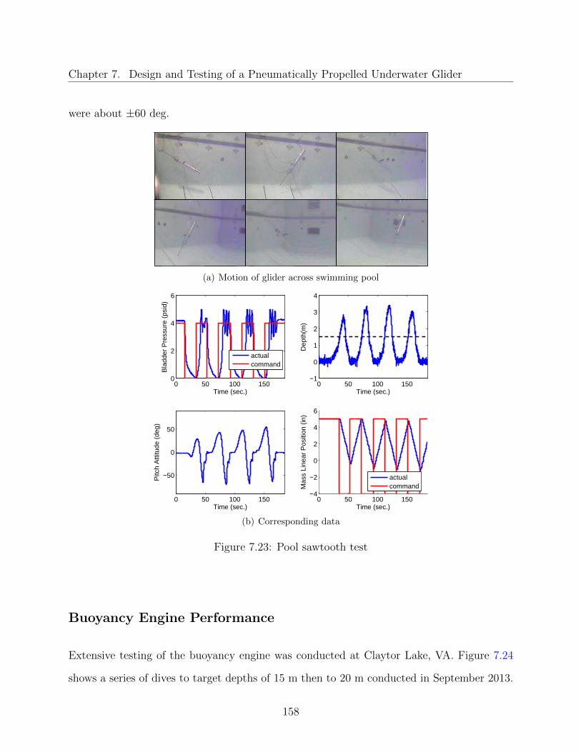
Chapter 7. Design and Testing of a Pneumatically Propelled Underwater Glider
were about ±60 deg.
(a) Motion of glider across swimming pool
0 50 100 150−4
−2
0
2
4
6
TimeD(sec.)
Mas
sDLi
near
DPos
ition
D(in
)
actualcommand
0 50 100 150
−50
0
50
TimeD(sec.)
Pitc
hDA
ttitu
deD(
deg)
0 50 100 150−1
0
1
2
3
4
TimeD(sec.)
Dep
th(m
)
0 50 100 1500
2
4
6
TimeD(sec.)
Bla
dder
DPre
ssur
eD(p
sid)
actualcommand
(b) Corresponding data
Figure 7.23: Pool sawtooth test
Buoyancy Engine Performance
Extensive testing of the buoyancy engine was conducted at Claytor Lake, VA. Figure 7.24
shows a series of dives to target depths of 15 m then to 20 m conducted in September 2013.
158

Chapter 7. Design and Testing of a Pneumatically Propelled Underwater Glider
In these experiments the inflator command was saturated to 30 % to prevent excessively fast
inflations. Dives to 20 m had about 3-4 m of overshoot and resulted in a change in tank
pressure of about 70 psi.
0 5 10 15 200
5
10
15
20
25
Dep
thw(
m)
Timew(min.)0 5 10 15 20
0
1
2
3
4
5
Bla
dder
wPre
ssur
ew(p
sid)
Timew(min.)
actualcommand
0 5 10 15 201100
1200
1300
1400
1500
1600T
ankw
Pre
ssur
ew(p
sid)
Timew(min.)
rawfiltered
0 5 10 15 200
20
40
60
80
100
Timew(min).
Com
man
dw[%
]
delfatorinflator
Figure 7.24: Buoyancy engine tests at Claytor Lake, VA
Trim and Gain Tuning
The goal of “trimming” the glider is to achieve a desired weight, buoyancy, and balance (cen-
ter of buoyancy and gravity) that meets performance and stability requirements. Carefully
estimating the mass properties and locations of all components in the vehicle during the de-
tailed design and fabrication stage is essential to minimizing the amount of trim adjustments
required once the vehicle is assembled. (Ideally this also includes a sensitivity analysis that
ensures the design is robust to small deviations in the expected values.)
The glider was trimmed for a number of operating conditions: the communication (“comms”)
stance (where the tail sticks above the water to improve reception, see Figure 7.28), a desired
159

Chapter 7. Design and Testing of a Pneumatically Propelled Underwater Glider
depth rate and pitch attitude during ascents or descents, and the ability to roll completely
around with one revolution of the moving mass. (Trimming is also required whenever a
major component is changed or when moving from fresh water to sea water and vice versa.)
A significant challenge encountered during trimming was the change in vehicle mass with
each dive (as air was exhausted from the tank). The sensitivity of the bladder pressure (and
the appropriate gains) to depth rate made gain tuning difficult. See Wolek et al. (2015c) for
a detailed discussion regarding the trim testing and gain tuning approach.
Figure 7.25: Glider in a communications stance
Acoustic LBL Ranging System
The acoustic LBL ranging system was tested in Claytor Lake, VA in November 2014. The ob-
jective of the experiment was to assess the performance of the system under ideal conditions
in the operating environment. The following discussion is adapted from (Gode, 2015).
The experiment consisted of deploying three mobile LBL nodes on rafts with transducers
submerged to 15 ft. The glider’s motion was emulated by keeping the glider aboard a moving
boat and submerging the transducer to 5 ft. Keeping the glider aboard the boat allowed us to
record the true GPS position of the glider relative to all of the deployed beacons (each logging
their own GPS position). Thus the accuracy of the LBL ranging system and resulting position
160

Chapter 7. Design and Testing of a Pneumatically Propelled Underwater Glider
estimates could be determined. For the purposes of this experiment only static estimation
algorithms were implemented. All of the data collected was processed offline. The host vessel
(and glider) were moved in a lawn mower pattern to cover a rectangular region in the vicinity
of the deployed beacons as shown in Figure 7.26.
Figure 7.26: Path of the boat (with onboard glider) during the test at Claytor Lake, VA(Map data from Google Earth). Used with permission (Gode, 2015).
The full track of the boat was divided into two separate tracks for analysis. The first track
(Track 1) comprised of the vertical (North-South) lawn mower paths (also called “swaths”).
Figure 7.27 shows the experimental results for Track 1. In Figure 7.27(a) the true range
(based on GPS positions) and measured range (based on travel time measurement, and
assumed speed of sound) are compared. The histogram in Figure 7.27(b) indicates that
about 75 % of attempted pings were successful. In regions of along the track were two or
more pings originated from unique beacons (as shown in Figure 7.27(c)), an estimate of the
position could be computed. The resulting estimates (Figure 7.27(d)) had an average error
of ≈ 10 m. A similar analysis was performed on the East-West track; see (Gode, 2015) for
161
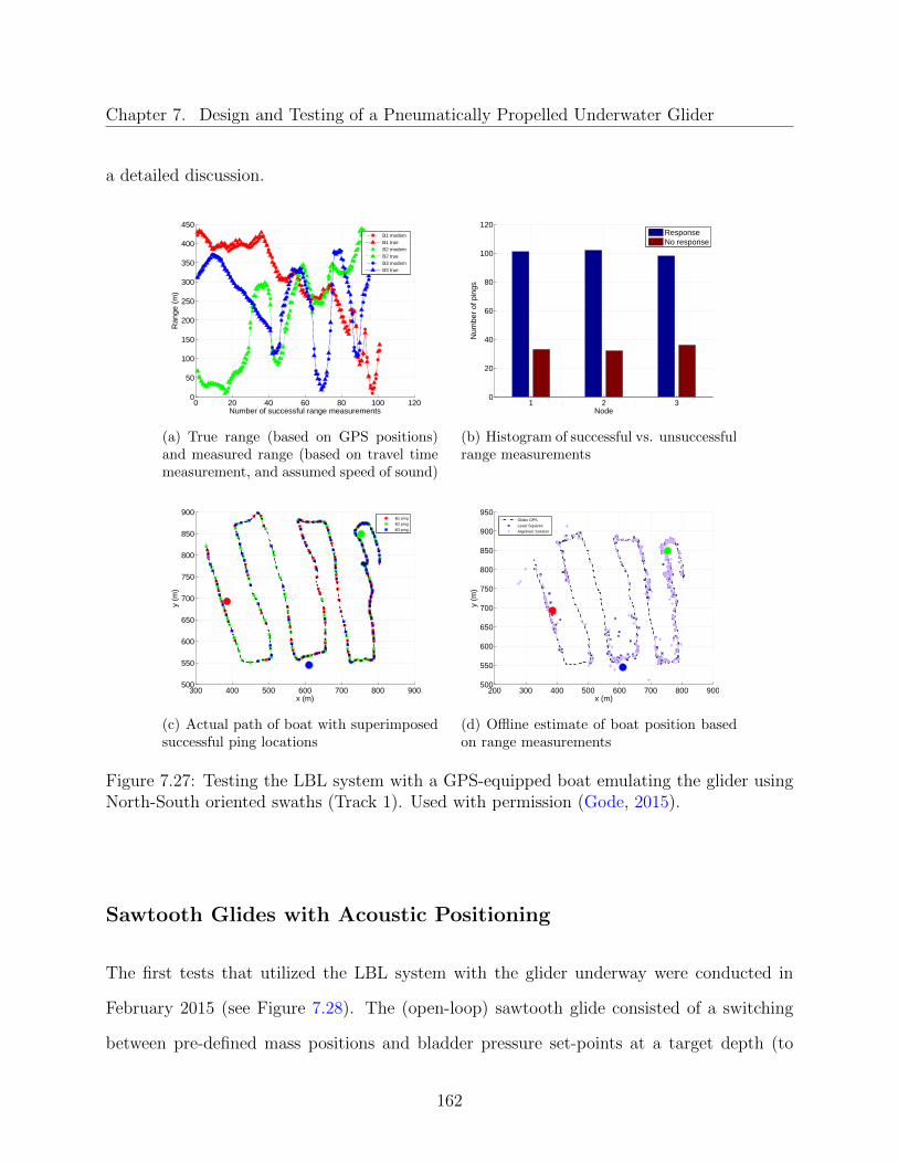
Chapter 7. Design and Testing of a Pneumatically Propelled Underwater Glider
a detailed discussion.
0 20 40 60 80 100 1200
50
100
150
200
250
300
350
400
450
Number of successful range measurements
Ran
ge (
m)
B1 modemB1 trueB2 modemB2 trueB3 modemB3 true
(a) True range (based on GPS positions)and measured range (based on travel timemeasurement, and assumed speed of sound)
1 2 30
20
40
60
80
100
120
Node
Num
ber
of p
ings
ResponseNo response
(b) Histogram of successful vs. unsuccessfulrange measurements
300 400 500 600 700 800 900500
550
600
650
700
750
800
850
900
x (m)
y (m
)
B1 ping
B2 ping
B3 ping
(c) Actual path of boat with superimposedsuccessful ping locations
200 300 400 500 600 700 800 900500
550
600
650
700
750
800
850
900
950
x (m)
y (m
)
Glider GPS
Least Squares
Algebraic Solution
(d) Offline estimate of boat position basedon range measurements
Figure 7.27: Testing the LBL system with a GPS-equipped boat emulating the glider usingNorth-South oriented swaths (Track 1). Used with permission (Gode, 2015).
Sawtooth Glides with Acoustic Positioning
The first tests that utilized the LBL system with the glider underway were conducted in
February 2015 (see Figure 7.28). The (open-loop) sawtooth glide consisted of a switching
between pre-defined mass positions and bladder pressure set-points at a target depth (to
162

Chapter 7. Design and Testing of a Pneumatically Propelled Underwater Glider
change from ascent to descent). Because there was no active pitch and roll control the glider
was unable to attain a steady level equilibrium glide. It was also observed during this test
that the acoustic ranging immediately ceased as the glider pitched down and began its dive.
This may be due to the transducer being mounted in the nose of the vehicle, and the body
of the vehicle interfering with the transducer’s operation.
Subsequent tests were conducted with closed-loop attitude feedback control to move the
internal mass, as shown in (see Figure 7.29). In these cases the transducer was mounted on
the the hull of the vehicle facing upwards however this did not improve the acoustic ranging
performance (no pings were successful during the sawtooth glide).
7.8 Conclusion
The design of an underwater glider with novel actuator capabilities was explored. The
feasibility of a novel pneumatic buoyancy engine was demonstrated. A cylindrical moving
mass actuator for unlimited roll control was designed to give the glider full roll control (the
ability to “flip over”) and make use of asymmetric geometries for improved hydrodynamic
efficiency. An acoustic long-baseline ranging system was developed to position the glider
while it was underway.
The buoyancy engine provided large displacements of up to 5 Liters and was shown
to operate reliably at depths up to 25 m. Unlike with legacy glider designs, the bladder
providing buoyancy is filled with a compressible gas (air) and is sensitive to changes in
ambient pressure (with depth). The large buoyancy engine may cause large and sudden
pitching moments that strongly affected the pitch attitude of the glider. It was found that
the bladder dynamics were much faster than that of the moving mass, making it difficult to
achieve a steady glide in the confines of a 25 m lake. Further, the change in mass of the
163

Chapter 7. Design and Testing of a Pneumatically Propelled Underwater Glider
(a) Visualization of glide orientation with depth and time: a circle indicatesa successful range measurement, circle’s color indicates range measurementfrom a unique beacon
12 12.5 13 13.5 140
5
10
15
20
25
Dep
th (
m)
Time (min.)12 12.5 13 13.5 14
−1
−0.5
0
0.5
1
Dep
th R
ate
(m/s
)
12 12.5 13 13.5 14
−7.5
−5
−2.5
0
2.5
5
7.5
Line
ar P
os. (
in.)
12 12.5 13 13.5 14−180
−90
0
90
180
Ang
ular
Pos
. (de
g)
Lin.PosLin.CmdRot.PosRot.Cmd
12 12.5 13 13.5 140
20
40
60
80
100
Time (min).
Com
man
d [%
]
DelfatorInflator
12 12.5 13 13.5 140
1
2
3
4
5
Bla
d. P
ress
. (ps
id)
Time (min.)
actualcommand
12 12.5 13 13.5 14−90
−45
0
45
90
Time (min.)
Ang
le (
deg.
)
PitchRoll
(b) Corresponding data
Figure 7.28: Sawtooth glide test with acoustic positioning
vehicle with each dive (as air was exhausted from the tank) made trimming difficult. The
ability to roll over with the cylindrical moving mass requires the glider to be trimmed such
164

Chapter 7. Design and Testing of a Pneumatically Propelled Underwater Glider
(a) Visualization of glide orientation with depth and time
1.4 1.6 1.8 2 2.2
0
5
10
15
Dep
th (
m)
Time (min.)1.4 1.6 1.8 2 2.2
−1
−0.5
0
0.5
1
Dep
th R
ate
(m/s
)
1.4 1.6 1.8 2 2.20
0.51
1.52
2.53
3.54
4.55
Line
ar P
os. (
in.)
1.4 1.6 1.8 2 2.2
100
120
140
Ang
ular
Pos
. (de
g)
Lin.PosLin.CmdRot.PosRot.Cmd
1.4 1.6 1.8 2 2.20
20
40
60
80
100
Time (min).
Com
man
d [%
]
DelfatorInflator
1.4 1.6 1.8 2 2.20
1
2
3
4
5
Bla
d. P
ress
. (ps
id)
Time (min.)
rawfiltercommand
1.4 1.6 1.8 2 2.2−180
−135
−90
−45
0
45
90
135
180
Time (min.)
Ang
le (
deg.
)
YawPitchRollPitch CmdRoll Cmd
(b) Corresponding data
Figure 7.29: Sawtooth glide test with acoustic positioning and attitude control
that the vehicle center of gravity (not including the moving mass) and center of buoyancy
are aligned in the vertical plane. Such a configuration implies that the bottom-heaviness
165

Chapter 7. Design and Testing of a Pneumatically Propelled Underwater Glider
of the vehicle is strictly a function of the rotating mass weight and position, and therefore
the bottom-heaviness is relatively small. This makes the glider more maneuverable (but
also less stable). It was found that rolling the glider on the surface is challenging due to
the discontinuous change in buoyancy of one of the wings during such a maneuver (and the
associated restoring moment), and also due to the effect of winds acting on the wing. The
acoustic long-baseline ranging system was found to work reliably when the transducers was
suspended in the water, however mounting the transducer on the vehicle strongly interfered
with its operation. Through these experimental efforts a number of challenges were identified
that may help inform future shallow water glider designs.
166

Chapter 8
Conclusions
Using optimal control theory, several novel micro-scale path planning approaches have been
developed. In the problems considered, the objective was to reach a desired planar posi-
tion and final heading angle with minimum cost. This work may be viewed as an extension
of the Dubins (1957) path planning problem, where the motion model and objectives are
reformulated to address shallow water operational challenges faced by underwater gliders.
Throughout a mission, changing environmental conditions and objectives may call for a num-
ber of varied (possibly even conflicting) planning approaches to be employed. Accordingly,
a range of planning problems have been considered that collectively address many of the
challenges expected in the shallow water environment; see Figure 8.1.
In the presence of unknown and unsteady currents, an approach was proposed for con-
structing modified Dubins paths that remain feasible for the glider. However, since the
disturbance is typically unknown these paths cannot be tracked perfectly. Instead, the re-
sulting paths reserve control authority that enables convergence to the desired path. Through
a Monte Carlo numerical investigation it was shown that this approach minimizes the mean
final cross-track error. This property of a path planning algorithm may be useful when
167

Chapter 8. Conclusions
VeryvShallowvWaters:vMin-DepthvPlanning
SignificantvCurrents:RobustvPlanning
TimevSensitivevMission:Min-TimevPlanning
Figure 8.1: Varying environmental conditions and objectives may require a number of dif-ferent planning approaches to be employed.
reaching a terminal state reliably is important.
For the case where transit time is a priority (e.g. when a quick maneuver is required to
avoid running aground) the minimum-time problem was considered. In the minimum-time
problem a central idea was the use of “cornering” extremal turns (where the glider briefly
operates at a reduced speed to turn sharply). By applying the Minimum Principle, and
from additional geometric considerations, a finite and sufficient set of candidate paths for
a globally optimal path was derived. A path synthesis approach that seeks the lowest cost
path within this set was then developed.
The problem of constructing energy-optimal paths that maximize range was also inves-
tigated. Operating in shallow waters necessitates performing energy-intensive buoyancy
changes more frequently and motivates planning such efficient paths. This problem was con-
sidered for the case of shallow bank angles (where the sink rate is approximated as quadratic
with speed), and for a more realistic model with this restriction removed where the sink rate
and turn rate are coupled. The first approach was amenable to more rigorous analysis, while
the latter approach provided a more realistic (but less tractable) model. Both problems gave
insight regarding the nature of optimal gliding turns.
168

Chapter 8. Conclusions
Last, the design of a novel underwater glider with improved capabilities was explored.
A prototype glider was fabricated with a pneumatic buoyancy engine (that allows for large,
rapid buoyancy changes) and a fast cylindrical moving mass mechanism (that generates large
pitch and roll moments to improve attitude control). Through field testing several advantages
and challenges associated with the proposed design were identified that may inform future
shallow water glider designs.
169
Appendix A
Deriving the Feasible Turn Radius R′0
The following derivations supplement Chapter 3 and are adapted from (Wolek and Woolsey,
2012, 2015a).
Proposition A.1. Given δ(t) ≤ δmax and ψδ(t), a circular turn of radius
R′0 = R0(1 + ε)2
is feasible for the system (3.2).
Proof. The radius of curvature R(t) of the path defined by the trajectory (x(t), y(t)) of
equations (3.2) in FI is
R(t) =(x2 + y2)3/2
|xy − yx|(A.1)
Noting that
x = −v sin(ψ)u+ δ cos(ψδ)− δ sin(ψδ)ψδ
y = v cos(ψ)u+ δ sin(ψδ) + δ cos(ψδ)ψδ
170
Appendix A. Deriving the Feasible Turn Radius R′0
and substituting into (A.1)
R(t) =ϕ3
|uϕ1 + ϕ2|
where
ϕ1 = v2 + vδ cos(ψ − ψδ)
ϕ2 = δ2ψδ − vδ sin(ψ − ψδ) + vδ cos(ψ − ψδ)ψδ
ϕ3 = (v2 + δ2 + 2vδ cos(ψ − ψδ))3/2
Observe that ϕ1 > 0 and ϕ3 > 0, given condition (3.1). Using the triangle and Cauchy-
Schwarz inequalities, recalling the input constraint, and rearranging gives
ϕ3
R(t)ϕ1
−∣∣∣∣ϕ2
ϕ1
∣∣∣∣ ≤ |u| ≤ v
R0
It follows that the range of attainable curvature is
R(t) ≥ R0ϕ3
vϕ1 +R0|ϕ2|(A.2)
Assume that there exists an upper bound on the right hand side (RHS) term of (A.2) and
denote this as upper bound R′0. Then it follows that the inertial turn radius R(t) can always
be made equal to or greater than R′0 by using a feasible control input. Hence, R′0 is the
“feasible turn radius” – the smallest possible turn radius that can be feasibly tracked.
To find this upper bound R′0 proceed by maximizing the RHS of (A.2). Note that the
RHS will be maximized if ϕ2 = 0. Since the terms δ and ψδ do not appear elsewhere, ϕ2 can
be equal to zero independently of ϕ1 and ϕ3. This occurs, for example, when the disturbance
171

Appendix A. Deriving the Feasible Turn Radius R′0
is constant in magnitude and direction (δ = 0 and ψδ = 0), but it also occurs in other cases
where the disturbances take certain “pathological” forms. With ϕ2 = 0 the RHS of (A.2)
becomes
R0ϕ3
vϕ1
=R0(v2 + 2vδ cos(ψ − ψδ) + δ2)3/2
v(v2 + vδ cos(ψ − ψδ))(A.3)
For any δ, the maximum of (A.3) occurs when cos(ψ − ψδ) = 1, this corresponds to a
situation where the disturbance is always aligned with the vehicle’s motion. Then (A.3)
simplifies to
R0(v + δ)2
v2
which is maximum when the disturbance magnitude is largest, δ = δmax. Defining
R′0 = max
(R0ϕ3
vϕ1 +R0|ϕ2|
)= R0
(v + δmax)2
v2
= R0(1 + ε)2
yields the result.
Corollary A.1. For δmax < V , a straight path is feasible for the system (3.2).
Corollary A.1 follows immediately from Proposition A.1 because R → ∞ for a straight
path.
Proposition A.2. A Dubins path constructed for the system (2.10) using the turn radius
R′0 is feasible for the system (3.2).
Proof. In Proposition A.1 and Corollary A.1 it was shown that (inertial) circular segments of
radius R′0 and (inertial) straight segments are feasible. Since Dubins paths comprise circular
172

Appendix A. Deriving the Feasible Turn Radius R′0
and straight segments, it follows that a Dubins path constructed for (2.10) using the turn
radius R′0 is feasible for the system (3.2).
The above results are extended to the case of steady uniform winds by adding constant
wind terms to the system (3.2) and considering motion in an air-relative frame. By adding
a steady uniform wind with magnitude w in the direction ψw, the system (3.2) becomes
x(t)
y(t)
ψ(t)
=
v cosψ(t) + δ(t) cosψδ(t) + w cosψw
v sinψ(t) + δ(t) sinψδ(t) + w sinψw
u(t)
(A.4)
To ensure a feasible solution w + δmax < v is required.
Corollary A.2. For any ψδ(t) and δ(t) ≤ δmax with constant w such that w + δmax < v,
there exists a suitably large turn radius R′0 in the moving, air-relative reference frame FA,
that is feasible for the system (A.4). The feasible turn radius is R′0 = R0(1 + ε)2 with ε
defined in (3.1).
Proof. Define the air-relative reference frame FA as an inertial frame that is convected in
the direction of the ambient wind ψw, at speed w. In the frame FA, the steady wind terms
vanish, and the system becomes
xA(t)
yA(t)
ψ(t)
=
v cosψ(t) + δ(t) cosψδ(t)
v sinψ(t) + δ(t) sinψδ(t)
u(t)
(A.5)
System (A.5) is of the same form as system (3.2), however xA and yA are air-relative positions.
Note that in FA, the minimum turn radius is still R0, and using the same approach described
173

Appendix A. Deriving the Feasible Turn Radius R′0
in the proof of Proposition A.1 the result is obtained that the feasible turn radius in the
moving, air-relative frame is R′0 = R0(1 + ε)2.
174
Appendix B
Sub-Optimality Conditions for
Minimum-Time Paths
B.1 Analytical Approach to the min-H Operation
In Section 4.4, the Minimum Principle was interpreted geometrically using the hodograph.
While the hodograph gives insight regarding the extremal controls, it does not provide a
complete characterization. For example, analysis of the hodograph shows that when ηψ = 0,
the extremal control is along the maximum speed boundary, but the optimal turn rate is
indeterminate. Similarly, the hodograph shows that when η0|ηψ |
= umax, the maximum turn
rate constraint is active, but the corresponding speed is indeterminate. Here, an analytical
approach is used to complete the characterization of the extremal controls. Control pairs
(κ, v) are sought that minimize Hc in (5.11) subject to the constraints (5.6). Take the
system Lagrangian to be the control-dependent portion of the Hamiltonian, with the input
175

Appendix B. Sub-Optimality Conditions for Minimum-Time Paths
constraints appended using Lagrange multipliers:
L =Hc(η0, ηψ, κ, v) + µ1(v − 1) + µ2
(κ− umax
v
)+ µ3(vmin − v)
=η0
(1
v
)+ ηψκ+ µ1(v − 1) + µ2
(κ− umax
v
)+ µ3(vmin − v) .
The Lagrange multipliers µ1, µ2, µ3 are sometimes called Valentine multipliers, after F. A.
Valentine who studied such inequality constraints in the context of the calculus of variations
(Valentine, 1937). The Karush-Kuhn-Tucker (KKT) conditions (Gill et al., 1981) for the
extremal controls are:
dLdκ
= ηψ + µ2 = 0 , (B.1)
dLdv
= η0
(−1
v2
)+ µ1 + µ2
(umax
v2
)− µ3 = 0 , (B.2)
along with sign conditions µ1, µ2, µ3 ≥ 0, depending on whether the corresponding constraint
is active.
Case 1: No constraints active. With µ1 = µ2 = µ3 = 0, the KKT condition (B.1) gives
ηψ = 0 and (B.2) gives −η0/v2 = 0. Therefore η0 = 0, since v 6= 0, and the Hamiltonian
is written H = η cos(θ − ψ). For a non-trivial solution to the adjoint equation, η 6= 0 is
required and therefore the necessary condition H = 0 implies that cos(θ − ψ) = 0 and so
the heading is constant. With κ = 0 the cost functional (6.22) is clearly minimized for a
fixed speed v = 1. However this corresponds to an active maximum speed constraint, and
this case is not under consideration. Therefore if an optimal control exists, it lies on the
boundary of the admissible control set Ω where one or more constraints are active.
Case 2: Maximum speed constraint active (only). In this case, µ2 = µ3 = 0 and v = 1.
A necessary condition for optimality is H = η0 + η cos(θ − ψ) = 0, which can hold only if
176

Appendix B. Sub-Optimality Conditions for Minimum-Time Paths
the heading is constant (i.e., κ = 0), corresponding to a straight line segment traversed at
maximum speed. Note that η0 = 0 is admissible.
Case 3: Maximum speed and turn rate constraints active. If µ3 = 0, v = 1 and κ = umax,
the KKT conditions (B.1) and (B.2) become
ηψ + µ2 = 0 , (B.3)
−η0 + µ1 + µ2umax = 0 . (B.4)
Since µ2 > 0 then ηψ < 0 is required. Note that η0 6= 0 and divide (B.4) by (B.3)
η0
|ηψ|= umax +
(µ1
µ2
)> umax ,
and the result obtained by the hodograph is confirmed.
Case 4: Maximum turn rate constraint active (only). In this case, µ1 = µ3 = 0, κ =
umax/v and v ∈ (vmin, 1). The KKT conditions (B.1) and (B.2) become
ηψ + µ2 = 0 , (B.5)
η0
(−1
v2
)+ µ2
(umax
v2
)= 0 , (B.6)
yielding η0 + umaxηψ = 0. This can only hold for a constant ηψ. If this condition occurs
at isolated points it may be ignored. However, if it occurs over an interval, then η′ψ(s) =
η sin(ψ − θ) = 0, and either η = 0 or sin(ψ − θ) = 0. If η = 0, then a necessary condition is
H = η01
v+ ηψumax = 0 .
Substituting η0 = −umaxηψ gives v = 1, which is not the case under consideration here. The
177
Appendix B. Sub-Optimality Conditions for Minimum-Time Paths
condition sin(ψ − θ) = 0 holds for a given heading angle (ψ = θ ± kπ for k ∈ Z+) and
therefore can only occur at isolated points (since the turn rate is nonzero at these points).
Therefore this case can be ignored.
Case 5: Maximum turn rate and minimum speed constraints active. In this case, µ1 = 0,
v = vmin and κ = umax/vmin. The KKT conditions (B.1) and (B.2) become
ηψ + µ2 = 0 , (B.7)
η0
(−1
v2min
)+ µ2
(umax
v2min
)− µ3 = 0 . (B.8)
Since µ2 > 0 then ηψ < 0. Dividing (B.8) by (B.7),
η0
|ηψ|= umax −
(µ3
µ2
)v2
min < umax ,
and the result obtained from the hodograph is confirmed. Note that η0 = 0 is admissible.
Case 6: Minimum speed constraint active (only). In this case, µ1 = µ2 = 0, v = vmin and
κ ∈ [0, umax/vmin). The KKT conditions (B.1) and (B.2) becomes
ηψ = 0 , (B.9)
η0
(−1
v2min
)+ µ3 = 0 . (B.10)
The necessary condition H = η0/vmin + η cos(θ−ψ) = 0 implies that the heading is constant
(κ = 0). Referring to the hodograph, one sees that the locus defining the minimum speed
constraint is parallel to the separating plane P at the maximum speed constraint, which
corresponds to a lower valued Hamiltonian. Hence, straight line motion at minimum speed
is suboptimal.
178

Appendix B. Sub-Optimality Conditions for Minimum-Time Paths
Figure B.1: Symmetric turn with α = αsubopt
B.2 Sub-Optimality Conditions for Symmetric Turns
TFS and TRS
Consider a generic counter-clockwise (left) symmetric turn illustrated in Figure B.1, where
the arcs>AB,
>BC and
>CD correspond to the B, C and B arcs, subtending angles α, β, and
α respectively. Let the heading angle at point A be ψ. The cost of the path from A to
D along these arcs is JABCD = R(2α + β). For sufficiently large α, there may exist an
alternate and lower cost C arc (>AD in Figure B.1), subtending an angle δ that connects A
to D. If this arc exists then δ < π and the cost of traversing this path is JAD = Rδ. Any
self intersecting curve, such as>ABCD, corresponds to a heading change greater than π and
therefore JAD < JABCD. Let α = αsubopt give the angle of the smallest arc for which this
alternate (lower cost) C arc exists. Considering the triangle 4EHG, one finds that
sin δ/2
sin β/2=R− rR + r
. (B.11)
179
Appendix B. Sub-Optimality Conditions for Minimum-Time Paths
Summing the internal angles gives π = αsubopt + δ/2 + β/2 and with (B.11)
αsubopt = π − β
2− asin
(sin
β
2
(R− rR + r
)). (B.12)
The heading change for this suboptimal symmetric turn is ∆ψsubopt = 2αsubopt + β. To show
that ∆ψsubopt < 2π, consider the inequality
∆ψsubopt − 2π = −2asin
(sin
(β
2
)R− rR + r
)< 0 . (B.13)
Since BCB turns are being considered, β > 0 is required. It is clear that the argument of
asin in (B.13) is always positive and less than unity. Thus (B.13) holds in general for all
optimal symmetric turns. Referring to Table 4.2, it follows that that since TFS and TSS turns
have ∆ψ = 2π they are suboptimal.
B.3 Sub-Optimality Conditions for ST FB and TFBS Ex-
tremals
Consider a ST FB extremal that involves a switch from a straight line S segment to a TFB
turn that ends at the goal state – a fixed point located a horizontal distance ∆x and a
vertical distance ∆y away from the switching point, and with final heading ψ. (Assume the
initial heading is ψ0 = 0.) If there exists a family of extremal arcs ST FB to the goal state
(where the turns are less than one revolution), then the costs along the TFB turn segments
of each of these paths are equal since the heading change is fixed. (The cost is J = R|ψ|.)
Therefore, the minimum cost maneuver will be the one that minimizes the length of the S
segment, or equivalently, maximizes ∆x. Using (4.18) and (4.19), with a fixed final heading
180

Appendix B. Sub-Optimality Conditions for Minimum-Time Paths
ψ = α + β + γ, the displacement from the ST FB switching point to the goal state is given
by:
∆x(α, β) = (R− r)(sinα− sin(α + β)) +R sinψ , (B.14)
∆y(α, β) = (R− r)(cos(α + β)− cosα) +R(1− cosψ) . (B.15)
The optimization problem is to maximize (B.14) subject to the constraint (B.15). Note that
the solution to this problem also applies to TFBS extremal segments since these are simply
ST FB segments that are traversed in reverse between the same boundary conditions. The
solution also applies to right turns, however only left turns are considered here.
Range of ∆y. Before proceeding with the optimization problem, the range of admissible
∆y(α, β) is determined from (B.15), for a given ψ. This is equivalent to finding the minima
and maxima of the function g(α, β) = cos(α+ β)− cosα, since ∆y is obtained from g(α, β)
by scaling g(α, β) by a factor (R − r) > 0 and shifting it by the constant R(1− cosψ) ≥ 0.
Figure B.2 shows a contour plot of the function g(α, β) over the domain (α, β) ∈ [0, 2π] ×
[0, 2π].
Case 1: ψ ≤ π. The set of feasible (α, β) given the condition 0 ≤ γ ≤ α in a left symmetric
boundary turn can be expressed as the region between the solid line 2α + β = ψ (for the
case when γ = α) and the dashed line α+ β = ψ (for the case when γ = 0). The triangular
region defined by these lines gives the feasible set as shown in Figure B.2 for Case 1. It is
trivial to show that the minimum of g(α, β) in this feasible set occurs at (α, β) = (0, ψ) and
the maximum occurs at (α, β) = (ψ, 0) where g(α, β) = 0. Thus the bounds of ∆y for ψ ≤ π
are given by
r(1− cosψ) ≤ ∆y ≤ R(1− cosψ) , (B.16)
and these correspond to following a pure B arc or a pure C arc as shown in Figure B.3.
181

Appendix B. Sub-Optimality Conditions for Minimum-Time Paths
0
1.5708
3.1416
4.7124
6.2832
0
1.5708
3.1416
4.7124
6.2832
−1
0
1
Figure B.2: Contours of g(α, β) with the feasible set indicated as the triangular region, forψ ≤ π, and as the trapezoidal region for ψ > π
Figure B.3: Admissible ∆y for ψ ≤ π
182

Appendix B. Sub-Optimality Conditions for Minimum-Time Paths
Figure B.4: Admissible ∆y for ψ > π
Case 2: ψ > π. If ψ > π the additional constraint for a flexible boundary turn 2α+β < 2π
is required so that the change in heading is less than 2π. This additional constraint (shown
as dashed-dotted line in Figure B.2) bisects the triangular region formed by the previous
constraints to form a trapezoidal shaped feasible set. The critical points of the unconstrained
function g(α, β) occur outside this feasible set. Thus the minimum and maximum values are
sought along the boundaries. After some analysis, one finds that for ψ > π the minimum
of g(α, β) occurs at (α, β) = (ψ−π2, π) with γ = α and the maximum at (α, β) = (ψ, 0) with
γ = 0. The bounds for ∆y are then
− 2(R− r) sin
(ψ
2
)+R(1− cosψ) ≤ ∆y ≤ R(1− cosψ) , (B.17)
corresponding to the cases shown in Figure B.4.
Maximizing ∆x. Consider only the admissible ∆y that satisfy the bounds derived in
the previous sections for a given ψ. Appending the constraint (B.15) to (B.14) using the
multiplier λ gives the Lagrangian
L(α, β, λ) =(R− r)(sinα− sin(α + β)) +R sinψ + λ[∆y − (R− r)(cos(α + β)− cosα)−R(1− cosψ)] .
183
Appendix B. Sub-Optimality Conditions for Minimum-Time Paths
The necessary conditions for a stationary point are
∂L(α, β, λ)
∂α=(R− r)[cosα− cos(α + β) + λ(sin(α + β)− sinα)] = 0 ,
and
∂L(α, β, λ)
∂β=(R− r)[λ sin(α + β)− cos(α + β)] = 0 . (B.18)
Equating ∂L∂α
= ∂L∂β
gives the multiplier λ = cot α and substituting into (B.18) the condition
for a stationary point is
sin β = 0 . (B.19)
If α = π then β = 0 and γ = ψ − α so that the solution corresponds to a pure B arc. The
optimization problem does not need to be considered for this case. If α 6= π a stationary
point exists and λ = cotα is well defined. For a flexible boundary turn, 2α+ β ≤ 2π is also
required.
Proceeding with α 6= π, (B.19) implies that the stationary points are (α, β, λ) = (α, 0, cotα)
and (α, β, λ) = (α, π, cotα). Comparing the value of ∆x for the case β = π and β = 0,
∆x(α, π)−∆x(α, 0) = 2(R− r) sinα > 0 ,
for all α < π. Thus β = π corresponds to a maximum and β = 0 corresponds to a minimum of
∆x. However, the set of admissible β for a given ∆y and ψ does not necessarily contain β = π
and so it is necessary to find conditions for maximizing ∆x when β = π is not admissible.
In the following, two cases for admissible β ∈ [βmin, βmax] are considered: βmax > π and
βmax < π. In both cases βmin is unknown.
Case 1: βmax > π. Let βmax = π + β0 with 0 < β0 < π, α = α0 ≤ π, and γ = γ0 ≤ α0.
184

Appendix B. Sub-Optimality Conditions for Minimum-Time Paths
Then ψ = α0 + π + β0 + γ0 and suppose these angles satisfy the constraint (B.15). Writing
all constants in the expression for ∆y on the left hand side, (B.15) becomes
∆y −R(1− cosψ)
(R− r)= − cos(α0 + β0)− cosα0 . (B.20)
Similarly, let the turn containing the stationary point β1 = π be parametrized such that
ψ = α1 + π + γ1. Then (B.15) becomes
∆y −R(1− cosψ)
(R− r)= −2 cosα1 . (B.21)
The expressions (B.20) and (B.21) are equal if
cosα1 =cos(α0 + β0) + cosα0
2, (B.22)
which always has a solution with α1 ≤ π and with α1 ≤ α0 + β0. Therefore if βmax > π is
an admissible solution to (B.15) then there is an alternate solution with β1 = π and with
admissible α1 satisfying (B.22) and
γ1 = ψ − π − α1 = α0 + β0︸ ︷︷ ︸≥α1
−α1 + γ0 ≥ γ0 .
For γ1 to be admissible α1 ≥ γ1 is required, and since ψ = α1 + π + γ1
α1 − γ1 = ψ − π − 2γ1 ≥ ψ − π − 2γ0 . (B.23)
Also since ψ = α0 +π+β0 +γ0 ≥ π+β0 +2γ0, substituting into (B.23) gives α1−γ1 ≥ β0 > 0
and so γ1 is admissible. Thus it has been shown that, in general, if β = βmax > π is an
admissible solution, then β = π is also admissible, and since β = π maximizes ∆x it is the
185

Appendix B. Sub-Optimality Conditions for Minimum-Time Paths
Figure B.5: Suboptimal case: β > π
optimal solution. This optimality property is illustrated graphically in Figure B.5, where for
both β > π and β < π the distance ∆x is smaller than it is for the optimal value β = π
where ∆x is maximized.
Case 2: βmax < π. Since β = π is a maximum and β = 0 is a minimum of ∆x, and ∆x is
increasing with β on the interval β ∈ [0, π] the optimal value of β ∈ [βmin, βmax] is βmax. In
the following, it is shown that d∆xdγ
< 0 when β < π and therefore that γ should be minimized
to maximize ∆x. To compute d∆xdγ
first differentiate both sides of (B.15) with respect to γ:
d∆y
dγ=(R− r)
[− sin(α + β)
(dα
dγ+dβ
dγ
)+ sinα
(dα
dγ
)]= 0 . (B.24)
Then from the relation α + β + γ = ψ
dα
dγ+dβ
dγ+ 1 = 0 , (B.25)
and simplifying (B.24) using (B.25) gives
dα
dγ=− sin(α + β)
sinα, (B.26)
186

Appendix B. Sub-Optimality Conditions for Minimum-Time Paths
Figure B.6: Suboptimal case: γ > γmin
so that
d∆x
dγ= (R− r)
[cosα
(dα
dγ
)− cos(α + β)
(dα
dγ+dβ
dγ
)]= (R− r)
[cosα
(− sin(α + β)
sinα
)+ cos(α + β)
]= −(R− r)
(sin β
sinα
)< 0 ,
for all α < π and β < π. (Note that since ψ > π and β < π, α > 0 and the above expression
is well defined.) This case is illustrated in Figure B.6 where ∆x is largest when γ is minimum
and β is maximum. (Actually, in Figure B.6 γ is zero along the optimal path; γ = 0 is always
admissible, as shown in the following.)
Optimal ST FB paths for ψ ≤ π. If ψ ≤ π then βmax < π, and the range of admissible ∆y
is given by (B.16). The minimum and maximum boundaries of this range were constructed
with admissible controls that have γ = 0 corresponding to the dashed line in for Case 1 in
Figure B.2. Further, noting that every contour of g(α, β) in Figure B.2 intersects the dashed
line suggests that there is a solution to (B.15) with γ = 0 for every ∆y in the range (B.16).
This proof is omitted here for brevity. Thus there exists a solution with α, β, and γ = 0 for
all ∆y in the range (B.16), and when ψ < π the optimal ST FB path has γ = 0.
Optimal ST FB paths for ψ > π. If ψ > π then the range of admissible ∆y is given
187

Appendix B. Sub-Optimality Conditions for Minimum-Time Paths
Figure B.7: BTRSB segment with equal initial and final B arcs
by (B.17). Figure B.2 shows that in Case 2 there is always a solution corresponding to
the horizontal line where β = π extending between the solid and dashed-dotted line of the
trapezoidal feasible region. Again, note that every contour of g(α, β) in the feasible intersects
this line where β = π. The proof is omitted here for brevity. Therefore for every admissible
∆y, given ψ > π, there is a solution with β = π. Further, it has been shown that β = π
maximizes ∆x, this is the optimal solution.
B.4 Sub-Optimality Conditions for BT RSB Extremals
Consider a BTRSB segment with B arcs that subtend equal angles (as shown in Figure B.7).
Here, the conditions under which the arcs>AB and
>EF can be joined by a lower cost arc
are derived. Let the distance between the circle centers G and H be d. Denote the angles,
measured counter-clockwise from the centerline GH, to the beginning and end of>AB as θ1
and θ2 respectively. (The angle θ2 is therefore negative in Figure B.7.) Let the heading angle
at point B in Figure B.7 be ψ, so that θ1 = ψ−π/2. Since the vehicle is pointing east at the
188

Appendix B. Sub-Optimality Conditions for Minimum-Time Paths
midpoint of the C arc>CD, it follows that ψ−α−β/2 = 0. If all of the B arcs subtend equal
angles α, then θ1 − θ2 = α which gives θ1 = ψ − π/2 and θ2 = β/2− π/2. The distance ∆x
can be found from (4.18) (using negative angles for α, β and γ = α since it is a right turn,
and with ψ0 = α + β/2) to give
∆x = 2
((R− r) sin
(β
2
)−R sin
(α +
β
2
)).
Then summing the horizontal distances from G to H
d = 2R cos θ1 + ∆x = 2(R− r) sin
(β
2
),
which is independent of α and bounded: d ≤ 2(R− r). Consider the ways by which the arcs
>AB and
>EF can be joined with a single arc of radius ρ > r. If 0 < d ≤ 2(R + r), then there
exist two possible connecting arcs, starting either below or above the centerline (shown as
Case A in Figure B.8). If 0 < d < 2(R − r) there are additional arcs that lie within the
intersection of the two circles (shown as Case B in Figure B.8). Let the angles corresponding
to starting point of these two arcs be denoted θB and −θB. These angles are given by
cos θB =d
2(R− ρ)=
(R− rR− ρ
)sin
(β
2
). (B.27)
Note that θB is largest when ρ = r giving
cos θB,max = sin
(β
2
), (B.28)
and θB is smallest when ρ = R − d/2 so that θB,min = 0 (shown as Case C in Figure B.8).
If d = 0 then the two circles coincide and the problem is not well posed. The solution to
the case when the circles exchange sequence (d < 0) is given by symmetry. From (B.28) it
189
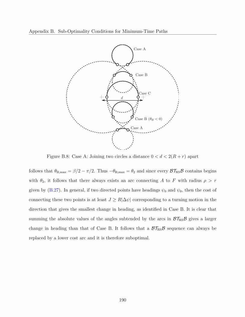
Appendix B. Sub-Optimality Conditions for Minimum-Time Paths
Figure B.8: Case A: Joining two circles a distance 0 < d < 2(R + r) apart
follows that θB,max = β/2− π/2. Thus −θB,max = θ2 and since every BTRSB contains begins
with θ2, it follows that there always exists an arc connecting A to F with radius ρ > r
given by (B.27). In general, if two directed points have headings ψ0 and ψ0, then the cost of
connecting these two points is at least J ≥ R|∆ψ| corresponding to a turning motion in the
direction that gives the smallest change in heading, as identified in Case B. It is clear that
summing the absolute values of the angles subtended by the arcs in BTRSB gives a larger
change in heading than that of Case B. It follows that a BTRSB sequence can always be
replaced by a lower cost arc and it is therefore suboptimal.
190

Appendix C
Minimum-Energy Extremals for a
Quadratic Glider Polar
C.1 Parameterizing Extremal Controls
The extremal controls are given in Table 5.1. If the glider employs a given extremal control
for some duration, the result will be a change in the state (heading and position) and cost
(altitude). To aid in further analysis, the extremal controls can be uniquely parametrized to
quantify such changes. Recall that an S extremal has speed v = vstf and turn rate u = 0.
This straight line path can be parametrized by its length L and heading angle ψi. In this
case, the state and cost rates are fixed, and the time to traverse the length L is simply L/vstf .
Thus the changes in heading (∆ψS), planar positions (∆xS and ∆yS), and altitude ∆hS , are
191

Appendix C. Minimum-Energy Extremals for a Quadratic Glider Polar
obtained by multiplying the fixed state and cost rates by the time interval L/vstf :
∆ψS(L, ψi) = 0 , (C.1)
∆xS(L, ψi) = L cosψi , (C.2)
∆yS(L, ψi) = L sinψi , (C.3)
∆hS(L, ψi) = L
(avstf + b+
c
vstf
). (C.4)
B extremal arcs have v = vms− λ cos(ψ− θ) and |u| = umax and can be parametrized by the
initial orientation ψi, the change in heading δ, and the parameters θ and λ. These extremals
correspond to a fixed turn rate and the independent variable may be changed from t to ψ
where dt = (sgn(δ)/umax)dψ. Then integrating the equations of motion (5.1)-(5.3) and the
cost functional (6.22) with respect to ψ, the changes in state and cost are obtained:
∆ψB(ψi, δ, θ, λ) = δ , (C.5)
∆xB(ψi, δ, θ, λ) = sgn(δ)
(vms[sin(ψi + δ)− sinψi] + 1
2λ[δ cos θ + cos(2ψi − θ + δ) sin δ]
umax
),
(C.6)
∆yB(ψi, δ, θ, λ) = sgn(δ)
(vms[cosψi − cos(ψi + δ)] + 1
2λ[δ sin θ + sin(2ψi − θ + δ) sin δ]
umax
),
(C.7)
∆hB(ψi, δ, θ, λ) =
(sgn(δ)
umax
)[(av2
ms + bvms + c+1
2aλ2)δ +
1
2aλ2 cos(2ψi − 2θ + δ) sin δ
+ λ(b+ 2avms)(sin(θ − ψi) + sin(ψi − θ + δ))
]. (C.8)
Likewise, Bstall (or Bms) extremal arcs have |u| = umax and v = vstall (or v = vms). Such
extremals can be parametrized by the initial orientation ψi, and the change in heading δ.
Choosing v appropriately, the changes in state and cost, for both Bstall and Bms extremal
192
Appendix C. Minimum-Energy Extremals for a Quadratic Glider Polar
arcs, are given by:
∆ψBmin/ms(ψi, δ, v) = δ , (C.9)
∆xBmin/ms(ψi, δ, v) = sgn(δ)
(v(sin(ψi + δ)− sinψi)
umax
), (C.10)
∆yBmin/ms(ψi, δ, v) = sgn(δ)
(v(− cos(ψi + δ) + cosψi)
umax
), (C.11)
∆hBmin/ms(ψi, δ, v) =
|δ|(av2 + bv + c)
umax
. (C.12)
C.2 Solving for BSB Extremals
In Appendix C.1 individual B arcs and S segments are parametrized to give the resulting
planar displacements and changes in heading resulting from each extremal control. However
in a BSB extremal sequence, the three consecutive extremals are related by additional con-
straints. (For example, the final heading of a given extremal must correspond to the initial
heading of the following extremal.) Let the first B arc begin with heading ψi = 0 and result
in a heading change δ = α. Recall that the S segment must have a heading ψ = θ + π, thus
α = θ + π. Further, if the S segment is of length L and the final B arc corresponds to a
heading change δ = γ, then the BSB extremal is uniquely defined. Also, for a BSB sequence
λ = vstf − vms, thus this constant is known. Hence the parameters α, L and γ are sufficient
to define a BSB extremal and all subsets thereof. To satisfy the boundary conditions, this
sequence must result in a final heading ψ1, thus a constraint is:
ψ1 = ∆ψB(0, α, α, λ) + ∆ψS(L, α) + ∆ψB(α, α, γ, λ)
= α + γ mod 2π . (C.13)
193
Appendix C. Minimum-Energy Extremals for a Quadratic Glider Polar
Similarly, for the final planar positions x1 and y1
x1 = ∆xB(0, α, α, λ) + ∆xS(L, α) + ∆xB(α, α, γ, λ)
=λ[αc(α) + s(α)] + 2vmss(α)
2umax
sgn(α) + Lc(α)
+λ[γc(α) + c(α + γ)s(γ)] + 2vms[s(α + γ)− s(α)]
2umax
sgn(γ) , (C.14)
y1 = ∆yB(0, α, α, λ) + ∆yS(L, α) + ∆yB(α, α, γ, λ)
=λαs(α) + 2vms[1− c(α)]
2umax
sgn(α) + Ls(α)
+λ4[c(α)− c(α− 2(α + γ)) + 2γs(α)] + vms[c(α)− c(α + γ)]
umax
sgn(γ) , (C.15)
where the shorthand notation c(·) = cos(·) and s(·) = sin(·) is used. The system of three
equations (C.13)-(C.15) has three unknowns (α,L, γ) and can be solved with a multi-variate
root finding routine. However, this solution procedure may be simplified by transcribing the
problem into a root solving problem for one parameter. One advantage of this approach
is that root-finding routines , such as chebfun developed by the University of Oxford
(Chebfun, 2013), are capable of reliable finding all roots of a single variable on a given
interval. The system (C.13)-(C.15) can be rearranged into the form:
f1(α,L, γ) cosα + k1 sinα + k2 sin γ = k3 , (C.16)
f1(α,L, γ) sinα + k4 cosα + k5 cos(α + 2γ) = k6 , (C.17)
α + γ mod 2π = ψ1 , (C.18)
where
f1(α,L, γ) = 2umaxL+ λ(|α|+ |γ|) , (C.19)
194

Appendix C. Minimum-Energy Extremals for a Quadratic Glider Polar
and the constants depend on the sign of α and γ, (corresponding to a given path orientation):
k1 = (λ+ 2vms)sgn(α)− 2vmssgn(γ) ,
k2 = λ sgn(γ) cosψ1 ,
k3 = 2umaxx1 − 2vms sinψ1sgn(γ) ,
k4 =(λ+ 4vms)sgn(γ)
2− 2vmssgn(α) ,
k5 = −λ sgn(γ)
2,
k6 = 2umaxy1 − 2vmssgn(α) + 2vms cosψ1sgn(γ) .
Assume that cosα 6= 0 and k3 − k1 sinα− k2 sin γ 6= 0, and note that for any nonzero triple
(α,L, γ) the term f1(α,L, γ) > 0. Then divide (C.17) by (C.16) to eliminate f1(α,L, γ):
sinα
cosα=k6 − k4 cosα− k5 cos(α + 2γ)
k3 − k1 sinα− k2 sin γ. (C.20)
Using (C.18) the constraint (C.20) can be rewritten as
g1(α) = sinα[k3 − k1 sinα− k2 sin(ψ1 − α)]− cosα[k6 − k4 cosα− k5 cos(2ψ1 − α)] = 0 .
(C.21)
The roots of g1(α) over the interval α ∈ (−2π, 2π) give candidate values for α, where positive
roots correspond to initial left turns and negative roots to initial right turns. For each
candidate α two candidate γ can be determined from (C.18), corresponding to a final left
turn (γ > 0) or a final right turn (γ < 0). Once a candidate α and γ have been found,
f1(α,L, γ) is computed from
f1(α,L, γ) =k3 − k1 sinα− k2 sin γ
cos(α),
195

Appendix C. Minimum-Energy Extremals for a Quadratic Glider Polar
and, lastly, L is determined from (C.19).
However, if cos(α) = 0 or k3 − k1 sinα − k2 sin γ = 0, then the previous assumptions do
not hold. Note that if k3 − k1 sinα − k2 sin γ = 0 then (C.16) implies that cosα = 0, thus
both conditions are equivalent. If cos(α) = 0 then the candidate α are ±π/2 or ±3π/2 and
the solution is algebraic (it is omitted here for brevity).
C.3 Solving for BBBB Extremals
Consider the class of BBBB candidate optimal controls, the first B arc begins with heading
ψi = 0 and subtends an angle α (where the sign of the angle represents the direction of
the turn). The next two B arcs in the sequence are anti-symmetric to each other. From
Lemma 5.7.8, if the second arc subtends an angle β, then θ = (2α+β)/2. Because the third
arc is antisymmetric to the first, the change in heading along this B arc is −β. Last, the final
arc subtends an angle γ. For this class and path type λ ≤ vstf−vstf and the parameter vector
p = (α β γ λ)T uniquely defines the sequence. Note that for a given path orientation
(for example, RLRL) the angles α, β, γ are constrained in sign and magnitude. Thus the
parameters must lie in a region defined by a polytope of the form Ap ≤ b. Using the
expressions in Appendix C.1, a constraint for the boundary conditions can be formulated as
g(p) =
x(p)− x1
y(p)− y1
ψ(p)− ψ1
= 0 ,
where xp = (x(p) y(p) ψ(p))T is the terminal state for a given parameter vector p. Further
the expressions for the change in altitude can be used to express the total cost J(p). Then
196
Appendix C. Minimum-Energy Extremals for a Quadratic Glider Polar
the constrained optimization problem is:
min J(p) , (C.22)
subject to Ap ≤ b ,
g(p) = 0 .
A numerical solver, such as fmincon, developed by MATLAB (2013), may return a locally
optimal solution to the problem (C.22), if one exists. Note that this formulation applies
only to BBBB sequences, however shorter sequences, such as BBB or BB will have different
constraints and they are not detailed here for brevity.
C.4 Solving for BstallBstallBstallBstall and Bms Extremals
Recall that the “middle”Bstall arcs in a BstallBstallBstallBstall sequence are anti-symmetric and
each correspond to heading changes |∆ψ| = π. If the first arc in this sequence subtends an
angle α, and the the final arc subtends an angle γ, then the sequence is uniquely defined by
these two parameters. Let k = sgn(α) denote the sign of initial turn (left or right). Then
the boundary conditions are:
x1 = ∆xBstall(0, α) + ∆xBstall(α,−kπ) + ∆xBstall(α− kπ, kπ) + ∆xBstall(α, γ) , (C.23)
y1 = ∆yBstall(0, α) + ∆yBstall(α,−kπ) + ∆yBstall(α− kπ, kπ) + ∆yBstall(α, γ) , (C.24)
ψ1 = α + γ . (C.25)
197

Appendix C. Minimum-Energy Extremals for a Quadratic Glider Polar
Using (C.23) and (C.25), the expression
sin(α) =x1umax
6kvstall
+sinψ1
6, (C.26)
gives α, and γ = ψ1 − α. Similarly, in a BstallBstallBstall sequence, let the initial Bstall arc
subtend α the middle arc subtend −kπ and the final arc subtend γ. In this case
sin(α) =x1umax
4kvstall
− sinψ1
4(C.27)
and γ = ψ1 − α + kπ. Likewise, for a BstallBstall sequence
sin(α) =x1umax
2kvstall
+sinψ1
2(C.28)
and, again, γ = ψ1−α. The case of a single Bstall or Bstall is trivial since the arc must subtend
an angle equal to the final heading ψ1.
198

Chapter 9
Bibliography
Adler, A., Bar-Gill, A., and Shimkin, N. (2012). Optimal Flight Paths for Engine-OutEmergency Landing. In Proceedings of the 24th Chinese Control and Decision Conference,pages 2908 – 2915, Piscataway, NJ. IEEE. 73
Allen, D. W., Jones, M. C., McCue, L. S., Woolsey, C. A., and Moore, W. B. (2013). Mappinga Mission Profile for the Exploration of Europa’s Ocean (AIAA 2013-5474). In Proceedingsof the AIAA SPACE 2013 Conference and Exposition, Reston, VA. AIAA. 3
Alvarez, A., Caiti, A., and Onken, R. (2004). Evolutionary Path Planning for Au-tonomous Underwater Vehicles in a Variable Ocean. IEEE Journal of Oceanic Engineering,29(2):418–429. 10
Anderson, R. P., Bakolas, E., Milutinovic, D., and Tsiotras, P. (2013). Optimal FeedbackGuidance of a Small Aerial Vehicle in a Stochastic Wind. Journal of Guidance, Control,and Dynamics, 36(4):975–985. 31
Anisi, D. A. (2003). Optimal Motion Control of a Ground Vehicle. Technical Report FOI-R–0961–SE, Swedish Defense Research Agency, Stockholm, Sweeden. 29
Atkins, E. M., Portillo, I. A., and Strube, M. J. (2006). Emergency Flight Planning Appliedto Total Loss of Thrust. Journal of Aircraft, 43(4):1205–1216. 3, 73
Bachmayer, R., Graver, J. G., and Leonard, N. E. (2003). Glider Control: A Closer Lookinto the Current Glider Controller Structure and Future Developments. In Proceedings ofMTS/IEEE OCEANS 2003 Conference, pages 951–954, Piscataway, NJ. IEEE. 5
Bachmayer, R., Leonard, N. E., Graver, J. G., Fiorelli, E., Bhatta, P., and Paley, D. (2004).Underwater Gliders: Recent Developments and Future Applications. In Proceedings of the2004 International Symposium on Underwater Technology, pages 195–200, Piscataway, NJ.IEEE. 2
199
Chapter 9. Bibliography
Bakolas, E. and Tsiotras, P. (2010). Time-Optimal Synthesis for the Zermelo-Markov-DubinsProblem: the Constant Wind Case. In Proceedings of the 2010 American Control Confer-ence, pages 6163 – 6168, Piscataway, NJ. IEEE. 7, 30, 33
Bakolas, E. and Tsiotras, P. (2011). Optimal Synthesis of the Asymmetric Sinistral/DextralMarkov-Dubins Problem. Journal of Optimization Theory and Applications, 150(2):233–250. 8
Bakolas, E. and Tsiotras, P. (2012). Feedback Navigation in an Uncertain Flowfield andConnections with Pursuit Strategies. Journal of Guidance, Control, and Dynamics,35(4):1268–1279. 9
Bhatta, P. (2006). Nonlinear Stability and Control of Gliding Vehicles. PhD thesis, PrincetonUniversity, Princeton, NJ. 5
Bhatta, P. and Leonard, N. E. (2008). Nonlinear Gliding Stability and Control for Vehicleswith Hydrodynamic Forcing. Automatica, 44(5):1240–1250. 5
Bingham, B. (2009). Navigating Autonomous Underwater Vehicles. In Underwater Vehicles,pages 33–50. InTech, Rijeka, Croatia. 153
Bloch, A. M. (2003). Nonholonomic Mechanics and Control. Interdisciplinary Applied Math-ematics, New York, NY. 27
Boissonnat, J.-D. and Bui, X.-N. (1994). Accessibility Region for a Car that Only MovesForwards Along Optimal Paths. Technical Report INRIA-2181, Institut National DeRecherche en Informatique en Automatique, Sophia-Antipolis, France. 34
Boissonnat, J.-D., Cerezo, A., and Leblond, J. (1992). Shortest Paths of Bounded Curvaturein the Plane. In Proceedings of the 1992 IEEE International Conference on Robotics andAutomation, pages 2315–2320, Piscataway, NJ. IEEE. 6, 28
Boissonnat, J.-D., Cerezo, A., and Leblond, J. (1994). A Note on Shortest Paths in the PlaneSubject to a Constraint on the Derivative of the Curvature. Technical Report INRIA-2160, Institut National De Recherche en Informatique en Automatique, Sophia-Antipolis,France. 7
Borchsenius, J. and Pinder, S. (2010). Underwater glider propulsion using chemical hydrides.In Proceedings of the IEEE OCEANS 2010 Conference, Sydney, Australia. 132
Boyd, J. R., Christie, T. P., and Drabant, R. E. (1971). Maximum Maneuver Concept. EglinAir Force Base, Air Force Armament Memorandum No. 71-2, Eglin AFB, Florida. 114
Breivik, M. and Fossen, T. (2008). Guidance Laws for Planar Motion Control. In Proceedingsof the 47th IEEE Conference on Decision and Control, pages 570–577, Piscataway, NJ.IEEE. 36, 38
200

Chapter 9. Bibliography
Brinkman, K. and Visser, H. G. (2007). Optimal Turn-Back Manoeuvre After Engine Failurein a Single-Engine Aircraft During Climb-Out. Proceedings of the Institution of MechanicalEngineers, Part G: Journal of Aerospace Engineering, 221(G):17–27. 72
Bui, X.-N., Boissonnat, J.-P., Soueres, P., and Laumond, J.-D. (1994). Shortest Path Syn-thesis for Dubins Non-Holonomic Robot. In Proceedings of the 1994 IEEE InternationalConference on Robotics and Automation, pages 2–7, Piscataway, NJ. IEEE. 7, 29, 34
Bullo, F. and Lewis, A. D. (2004). Geometric Control of Mechanical Systems. Springer-Verlag: Texts in Applied Mathematics, Number 49, New York-Heidelber-Berlin. 27
Burns, J. A. (2013). Introduction to The Calculus of Variations and Control with ModernApplications. Taylor & Francis Group, Boca Raton, FL. 14, 16
Cameron, C. G. (2005). The WET Buoyancy Engine: Controlling Buoyancy via Electro-chemistry. Technical Report TM-2005-2014, Defense Research and Development Canada,Dartmouth, Nova Scotia. 132
Chebfun (2013). ver. 4.2. Oxford University Mathematical Institute, Oxford, England. 194
Chern, J.-S. (1984). Isochrones for Maximum Endurance Horizontal Gliding Flight. Journalof Guidance, Control, and Dynamics, 8(1):1984–1986. 73
Chitsaz, H. and LaValle, S. M. (2007). Time-Optimal Paths for a Dubins Airplane. InProceedings of the 46th IEEE Conference on Decision and Control, pages 2379–2384, Pis-cataway, NJ. IEEE. 6
Choi, H. and Atkins, E. M. (2010). Smooth Transitions for a Turning Dubins Vehicle (AIAA2010-7551). In Proceedings of the AIAA Guidance, Navigation, and Control Conference,Reston, VA. AIAA. 8
Cliff, E. M., Kelley, H. J., and Lefton, L. (1982). Thrust-vectored Energy Turns. Automatica,18(5):559–564. 75, 102
Cliff, E. M., Seywald, H., and Bless, R. R. (1993). Hodograph Analysis in Aircraft TrajectoryOptimization. In Proceedings of the AIAA Guidance, Navigation, and Control Conference,pages 363–371, Reston, VA. ix, 22, 23, 24, 27, 110
Cliff, E. M., Well, K.-H., and Schnepper, K. (1992). Flight-Test Guidance for AirbreathingHypersonic Vehicles. In Proceedings of the AIAA Guidance, Navigation, and ControlConference, Reston, VA. AIAA. 75, 102
Creed, E., Mudgal, C., Glenn, S., Schofield, O., Jones, C., and Webb, D. (2002). Using a Fleetof Slocum Battery Gliders in a Regional Scale Coastal Ocean Observatory. In Proceedingsof MTS/IEEE OCEANS 2002 Conference and Exhibition, pages 320–324, Piscataway, NJ.IEEE. 128, 132
201

Chapter 9. Bibliography
Danewid, R. (1988). A Simple Approximation of the Best-Speed-To-Fly Theory. OSTIVInternational Journal of Technical Soaring, 12(3):83–88. 75
Davis, R. E., Eriksen, C. C., and Jones, C. P. (2002). Technology and Applications ofAutonomous Underwater Vehicles: Autonomous Buoyancy-Driven Underwater Gliders.Taylor & Francis Group, New York, NY. 128
Davis, R. E., Leonard, N. E., and Fratantoni, D. M. (2009). Routing Strategies for Under-water Gliders. Deep Sea Research Part II: Topical Studies in Oceanography, 56:173–187.9
Degtiariova-Kostova, E. (2006). The Planar Motion with Two Bounded Controls - the Ac-celeration and the Derivative of the Curvature. Technical Report INRIA-3444, InstitutNational De Recherche en Informatique en Automatique, Sophia-Antipolis, France. 42
Degtiariova-Kostova, E. and Kostov, V. (1998). Irregularity of Optimal Trajectories in aControl Problem for a Car-Like Robot. Technical Report INRIA-3411, Institut NationalDe Recherche en Informatique en Automatique, Sophia-Antipolis, France. 7
DG Flugzeugbau Gmbh (2010). Flight manual for the motorglider DG-1001M. TechnicalReport EASA.A.072, Bruchsal, Germany. x, 94, 95
Djath, K., Siadet, A., Dufaut, M., and Wolf, D. (1999). Navigation of a Mobile Robot byLocally Optimal Trajectories. Robotica, 17(5):553–562. 6
D’Spain, G. (2009). Final Report: Flying Wing Autonomous Underwater Glider for BasicResearch in Ocean Acoustics, Signal/Array Processing, Underwater Autonomous VehicleTechnology, Oceanography, Geophysics, and Marine Biological Studies. Technical Report0704, Office of Naval Research, Arlington, VA. 129
D’Spain, G., Jenkins, S., Zimmerman, R., Luby, J., and Thode, A. (2005). UnderwaterAcoustic Measurements with the Liberdade/X-Ray Flying Wing Glider. Journal of theAcoustical Society of America, 117(4):2624. 129
Dubins, L. E. (1957). On Curves of Minimal Length with a Constraint on Average Curvature,and with Prescribed Initial and Terminal Positions and Tangents. American Journal ofMathematics, 79(3):497–516. 6, 10, 11, 28, 51, 56, 77, 112, 167
Edwards, D. J. and Silberberg, L. M. (2010). Autonomous Soaring: The Montague Cross-Country Challenge. Journal of Aircraft, 47(5):1763–1769. 3
Eichhorn, M. (2010). Solutions for Practice-Oriented Requirements for Optimal Path Plan-ning for the AUV “Slocum Glider”. In Proceedings of the MTS/IEEE OCEANS 2010Conference, Piscataway, NJ. IEEE. 9
202

Chapter 9. Bibliography
Eng, P., Mejias, L., Walker, R., and Fitzgerald, D. (2010). Guided Chaos: Path Planning andControl for a UAV-Forced Landing. IEEE Robotics & Automation Magazine, 17(2):90–98.73
Eriksen, C. C., Osse, T. J., Light, R. D., Wen, T., Lehman, T. W., Sabin, P. L., Ballard,J. W., and Chiodi, A. M. (2001). Seaglider: A Long-Range Autonomous UnderwaterVehicle For Oceanographic Research. IEEE Journal of Oceanic Engineering, 26(4):424–436. 8, 132
Federal Aviation Administration (1987). Accident Prevention Program: Impossible Turn.Technical Report FAA-P-8740-44, Washington, D.C. 72
Fedotov, A., Patsko, V., and Turova, V. (2011). Recent Advances in Mobile Robotics: Reach-able Sets for Simple Models of Car Motion. InTech, Rijeka, Croatia. 42
Fernandez-Perdomo, E., Cabrera-Gamez, J., Hernandez-Sosa, D., Isern-Gonzalez, J.,Dominguez-Brito, A. C., Redondo, A., Coca, J., Ramos, A., Alvarez-Fanjul, E., and Gar-cia, M. (2010). Path Planning for Gliders Using Regional Ocean Models: Application ofPinzon Path Planner with the ESEOAT Model and the RU27 Trans-Atlantic Flight Data.In Proceedings of the IEEE OCEANS 2010 Conference and Exhibition, Piscataway, NJ.IEEE. 9
Finke, K. (1992). Comparison of Classical Speed To Fly Theory Using Second, Third, Fourthand Fifth Degree Polynomial Speed Polars. OSTIV International Journal of TechnicalSoaring, 16(3):78–76. 74
Fraichard, T. and Scheuer, A. (2004). From Reeds and Shepp’s to Continuous-CurvaturePaths. IEEE Transactions on Robotics and Automation, 20(6):1025–1035. 7
Gage, S. (2003). Creating a Unified Graphical Wind Turbulence Model from Multiple Spec-ifications (AIAA-2003-5529). In Proceedings of the AIAA Modeling and Simulation Tech-nologies Conference and Exhibition, Reston, VA. AIAA. 38
Garau, B., Bonet, M., Alvarez, A., Ruiz, S., and Pascual, A. (2009). Path Planning ForAutonomous Underwater Vehicles in Realistic Oceanic Current Fields: Application toGliders in the Western Mediterranean Sea. Journal of Maritime Research, 6(2):5–22. 9
Gill, P. E., Murray, W., and Wright, M. H. (1981). Practical Optimization. Academic Press,London, England. 24, 115, 176
Gode, T. (2015). Long Baseline Ranging Acoustic Positioning System. Master’s thesis,Virginia Polytechnic Institute and State University, Blacksburg, VA. xi, 153, 154, 155,160, 161, 162
Graver, J. (2005). Underwater Gliders: Dynamics, Control and Design. PhD thesis, Prince-ton University, Princeton, NJ. 5
203

Chapter 9. Bibliography
Halter, M. C. and Cliff, E. M. (1991). Optimal Energy-Heading Transients for an Air-breathing Hypersonic Vehicle. In Proceedings of the Guidance, Navigation, and ControlConference, Reston, VA. AIAA. 75, 102
Herisse, B. and Pepy, R. (2013). Shortest Paths for the Dubins’ Vehicle in HeterogeneousEnvironments. In Proceedings of the 52nd IEEE Conference on Decision and Control,pages 4504–4509, Piscataway, NJ. IEEE. 7
Hoffren, J. and Raivio, T. (2000). Optimal Maneuvering After Engine Failure (AIAA-2000-3992). In Proceedings of the AIAA Atmospheric Flight Mechanics Conference, pages 277–287, Reston, VA. AIAA. 72
Imlach, J. and Mahr, R. (2012). Modification of a Military Grade Glider for Coastal ScientificApplications. In Proceedings of MTS/IEEE OCEANS 2012 Conference, Piscataway, NJ.128
Jenkins, S. A., Humphreys, D. E., Sherman, J., Osse, J., Jones, C., Leonard, N., Graver,J., Bachmayer, R., Clem, T., Carroll, P., Davis, P., Berry, J., Worley, P., and Wasyl, J.(2003). Underwater Glider System Study. Technical Report 53, Scripps Institution ofOceanography. 5, 129
Kanakakis, V., Valavanis, K., and Tsourveloudis, N. C. (2004). Fuzzy-Logic Based Navigationof Underwater Vehicles. Journal of Intelligent and Robotic Systems, 40(1):45–88. 5
Kapaldo, A. J. (2005). Gyroscope Calibration and Dead Reckoning for an AutonomousUnderwater Vehicle. Master’s thesis, Virginia Polytechnic Institute and State University,Blacksburg, VA. 153
Kelley, H. J. and Lefton, L. (1972). Supersonic Aircraft Energy Turns. Automatica, 8(5):575–580. 114
Kraus, R. (2010). Analytical and Numerical Optimal Motion Planning for an UnderwaterGlider. PhD thesis, Virginia Polytechnic Institute and State University, Blacksuburg, VA.5
Kruger, D., Stolkin, R., Blum, A., and Briganti, J. (2007). Optimal AUV Path Planning forExtended Missions in Complex , Fast-Flowing Estuarine Environments. In Proceedings ofthe 2007 IEEE International Conference on Robotics and Automation, pages 4265–4270,Piscataway, NJ. IEEE. 10
Lee, E. B. and Markus, L. (1967). Foundations of Optimal Control Theory. John Wiley &Sons, New York, NY. 16, 26
Leitmann, G. (1981). The Calculus of Variations and Optimal Control. Plenum Press, NewYork, NY. 16
204
Chapter 9. Bibliography
Leonard, N. and Graver, J. (2001). Model-Based Feedback Control of Autonomous Under-water Gliders. IEEE Journal of Oceanic Engineering, 26(4):633–645. 5
MacCready, P. B. (1954). Optimum Airspeed Selector. In Soaring, pages 8–9, Hobbs, NM.The Soaring Society of America. 74, 75, 83
Maggiar, A. and Dolinskaya, I. S. (2014). Construction of Fastest Curvature-ConstrainedPaths in Direction-Dependent Media. Journal of Guidance, Control, and Dynamics,37(3):813–827. 7
Mahmoudian, N. (2009). Efficient Motion Planning and Control for Underwater Gliders.PhD thesis, Virginia Polytechnic Institute and State University, Blacksuburg, VA. 5
Mahmoudian, N., Geisbert, J., and Woolsey, C. A. (2010). Approximate Analytical TurningConditions for Underwater Gliders: Implications for Motion Control and Path Planning.IEEE Journal of Oceanic Engineering, 35(1):131–143. 6
MATLAB (2013). ver. 8.2.0. The MathWorks, Inc., Natick, Massachusetts. 65, 197
McGee, T. G. and Hedrick, J. K. (2007). Optimal Path Planning with a Kinematic AirplaneModel. Journal of Guidance, Control, and Dynamics, 30(2):629–633. 7, 30, 33
McNeely, R. L., Iyer, R. V., and Chandler, P. R. (2007). Tour Planning for an UnmannedAir Vehicle Under Wind Conditions. Journal of Guidance, Control, and Dynamics,30(5):1299–1306. 7, 30
Mide Technology Corporation (2015). MSUB II - Underwater Morphing for Buoyancy Con-trol. <http://www.mide.com/technology/msub.php> (accessed 05/10/2015). 133
Milgram, J. (2005). Climb Performance and Handicapping. In Skylines, Front Royal, VA.Skyline Soaring Club. 75
Morrow, M., Woolsey, C. A., and Hagerman, G. M. (2006). Exploring Titan with Au-tonomous, Buoyancy Driven Gliders. Journal of British Interplanetary Society, 59(1):27–34. 3
Pepy, R. and Herisse, B. (2014). An Indirect Method for Optimal Guidance of a Glider.In Proceedings of the 19th IFAC World Congress, pages 5097–5102, Kidlington, Oxford.IFAC. 7
Peterson, C. and Paley, D. (2011). Multivehicle Coordination in an Estimated Time-VaryingFlowfield. Journal of Guidance, Control, and Dynamics, 34(1):177–191. 32
Pontryagin, L. S., Boltyanskii, V. G., Gamkrelidze, R. V., and Mischcenko, E. F. (1962).The Mathematical Theory of Optimal Processes. Interscience Publishers, New York, NY.16
205

Chapter 9. Bibliography
Rao, A. V., Benson, D. A., Darby, C. L., Patterson, M. A., Francolin, C., Sanders, I.,and Huntington, G. (2010). Algorithm 902: GPOPS, A MATLAB Software for SolvingMultiple-Phase Optimal Control Problems Using the Gauss Pseudospectral Method. ACMTransactions on Mathematical Software, 37(2). 123
Rao, D. and Williams, S. (2009). Large-Scale Path Planning for Underwater Gliders in OceanCurrents. In Proceedings of the Australasian Conference on Robotics and Automation,Sydney, Australia. ARAA. 9
Reeds, J. and Shepp, L. (1990). Optimal Paths For a Car That Goes Both Forwards andBackwards. Pacific Journal of Mathematics, 145(2):357–393. 6, 21
Rhoads, B., Mezic, I., and Poje, A. C. (2013). Minimum Time Heading Control of Under-powered Vehicles in Time-varying Ocean Currents. Ocean Engineering, 66:12–31. 9
Rogers, D. F. (1995). Possible “Impossible” Turn. Journal of Aircraft, 32(2):392–397. 72
Sanfelice, R. and Frazzoli, E. (2008). On the Optimality of Dubins Paths Across HeterogenousTerrain. In Proceedings of the 11th Workshop on Hybrid Systems and Control, pages 457–470. Springer. 7
Scheuer, A. and Fraichard, T. (1997). Continuous-Curvature Path Planning for Car-LikeVehicles. In Proceedings of the 1997 IEEE/RSJ International Conference on IntelligentRobots and Systems, pages 997–1003, Piscataway, NJ. IEEE. 7
Shapira, I. and Ben-Asher, J. (1997). Near-Optimal Horizontal Trajectories for AutonomousAir Vehicles. Journal of Guidance, Control, and Dynamics, 20(4):735–741. 8
Sherman, J., Davis, R. E., Owens, W. B., and Valdes, J. (2001). The Autonomous Under-water Glider ‘Spray’. IEEE Journal of Oceanic Engineering, 26(4):437–446. 132
Smith, R. N., Schwager, M., Smith, S. L., Jones, B. H., Rus, D., and Gaurav, S. S. (2011).Persistent Ocean Monitoring with Underwater Gliders : Adapting Sampling Resolution.Journal of Field Robotics, 28(5):714–741. 9
Soueres, P. and Laumond, J.-P. (1996). Shortest Paths Synthesis for a Car-Like Robot. IEEETransactions on Automatic Control, 41(5):672–688. 7
Soulignac, M., Taillibert, P., and Rueher, M. (2009). Time-Minimal Path Planning in Dy-namic Current Fields. In Proceedings of the 2009 IEEE International Conference onRobotics and Automation, pages 2473–2479, Piscataway, NJ. IEEE. 9
Steinberg, A. M. and Stalford, H. L. (1973). On Existence of Optimal Controls. Journal ofOptimization Theory and Applications, 11(3):266–273. 77
206

Chapter 9. Bibliography
Sussmann, H. (1997). The Markov-Dubins Problem with Angular Acceleration Control.In Proceedings of the 36th IEEEE Conference on Decision and Control, Piscataway, NJ.IEEE. 7
Sussmann, H. and Tang, G. (1991). Shortest Paths for the Reeds-Shepp Car: A Worked OutExample of the Use of Geometric Techniques in Nonlinear Optimal Control. TechnicalReport SYCON-91-10, Rutgers Center for Systems and Control, Piscataway, NJ. 6, 28
Swagelok Company (2007). Valve Sizing. Technical Report MS-06-84-E. 141
Tang, G., Wang, Z., and Williams, A. (1998). On the Construction of an Optimal FeedbackControl Law for the Shortest Path Problem for the Dubins Car-like Robot. In Proceedingsof the 30th Southeastern Symposium on Systems Theory, pages 280–284, Piscataway, NJ.IEEE. 21, 29
Techy, L. (2011). Optimal Navigation in a Planar Time-Varying Flow: Zermelo’s ProblemRevisited. Intelligent Service Robotics, (4):271–283. 4, 9
Techy, L., Tomokiyo, R., Quenzer, J., Beauchamp, T., and Morgansen, K. (2010a). Full-ScaleWind Tunnel Study of the Seaglider Underwater Glider. Technical Report 206, Universityof Washington. 151
Techy, L. and Woolsey, C. A. (2009). Minimum-Time Path Planning for Unmanned Aerial Ve-hicles in Steady Uniform Winds. Journal of Guidance, Control, and Dynamics, 32(6):1736–1746. 7, 21, 30, 33
Techy, L., Woolsey, C. A., and Morgansen, K. A. (2010b). Planar Path Planning for FlightVehicles in Wind with Turn Rate and Acceleration Bounds. In Proceedings of the 2010IEEE International Conference on Robotics and Automation, pages 3240–3245, Piscat-away, NJ. IEEE. 7
Thomasson, P. G. and Woolsey, C. A. (2013). Vehicle Motion in Currents. IEEE Journal ofOceanic Engineering, 38(2):226–242. 5
Thompson, D. R., Chien, S., Yi, C., Li, P., Cahill, B., Levin, J., Schofield, O., Balasuriya,A., Petillo, S., Arrott, M., and Meisinger, M. (2010). Spatiotemporal Path Planning inStrong, Dynamic, Uncertain Currents. In Proceedings of the 2010 IEEE InternationalConference on Robotics and Automation, pages 4778–4783, Piscataway, NJ. IEEE. 9
US Department of Defense (1995). Flying Qualities of Piloted Aircraft. Technical ReportMIL-HDBK-1797. 38
Valentine, F. (1937). The Problem of Lagrange with Differential Inequalities as Added SideConditions. PhD thesis, University of Chicago, Chicago, IL. 25, 115, 176
207
Chapter 9. Bibliography
Walton E. Williamson Jr. (1979). Minimum and Maximum Endurance Trajectories for Glid-ing Flight in a Horizontal Plane. Journal of Guidance, Control, and Dynamics, 2(6):457–462. 73
Webb, D., Simonetti, P., and Jones, C. (2001). Slocum: an Underwater Glider Propelled byEnvironmental Energy. IEEE Journal of Oceanic Engineering, 26(4):447–452. 8, 132
Witt, J. and Dunbabin, M. (2008). Go with the Flow: Optimal AUV Path Planning inCoastal Environments. In Proceedings of the 2008 Australian Conference on Robotics andAutomation, Canberra, Australia. ARAA. 10
Wolek, A., Burns, J., Woolsey, C. A., Tech, V., Quenzer, J., Techy, L., and Morgansen, K. A.(2012). A Maneuverable , Pneumatic Underwater Glider. In Proceedings of the 2012 IEEEOCEANS Conference and Exhibition, Piscataway, NJ. IEEE. 130
Wolek, A., Cliff, E. M., and Woolsey, C. A. (2015a). Energy-Optimal Path Planning for aGlider with Speed and Load Factor Controls. in review. 11, 102
Wolek, A., Cliff, E. M., and Woolsey, C. A. (2015b). Time-Optimal Path Planning for aKinematic Car with Variable Speed Controls. in review. 11, 42
Wolek, A., Gode, T., Woolsey, C. A., Quenzer, J., and Morgansen, K. A. (2015c). Designand Testing of a Pneumatically Propelled Underwater Glider for Shallow Water. TechnicalReport VaCAS-2015-01, Virginia Center for Autonomous Systems, Blacksburg, VA. 130,148, 160
Wolek, A. and Woolsey, C. A. (2012). Disturbance Rejection in Dubins Path Planning. InProceedings of the 2010 American Control Conference, pages 4873–4878, Piscataway, NJ.IEEE. 31, 170
Wolek, A. and Woolsey, C. A. (2015a). Feasible Dubins Paths in Presence of Unknown,Unsteady Velocity Disturbances. Journal of Guidance, Control, and Dynamics, 38(4):782–787. 11, 31, 170
Wolek, A. and Woolsey, C. A. (2015b). Optimal Paths for a Sailplane with a QuadraticGlide Polar. in review. 11, 73
Yilmaz, N., Evangelinos, C., Lermusiaux, P. F. J., and Patrikalakis, N. (2008). Path Planningof Autonomous Underwater Vehicles for Adaptive Sampling Using Mixed Integer LinearProgramming. IEEE Journal of Oceanic Engineering, 33(4):522–537. 10
Young, L. C. (1969). Lectures on the Calculus of Variations and Optimal Control Theory.W. B. Saunders Co., Philadelphia. 26
Zermelo, E. (1931). Uber Das Navigationsproblem Bei Ruhender Oder Veranderlicher Wind-verteilung (en. About the Navigation Problem in Static or Variable Wind Distribution).Zeitschrift fur angewandte Mathematik und Mechanik, 11(2):114–124. 9
208

Chapter 9. Bibliography
Zhang, F., Tan, X., and Khalil, H. K. (2012). Passivity-Based Controller Design for Sta-blization of Underwater Gliders. In Proceedings of the 2012 American Control Conference,pages 5408–5413, Piscataway, NJ. IEEE. 5
Zhang, W., Inanc, T., Ober-Blobaum, S., and Marsden, J. (2008). Optimal TrajectoryGeneration for a Glider in Time-Varying 2D Ocean Flows B-spline Model. In Proceedingsof the 2008 IEEE International Conference on Robotics and Automation, pages 1083–1088,Piscataway, NJ. IEEE. 9
209