Optimal Portfolio Composition for SovereignWealth Funds

Khouzeima Moutanabbir* Diaa Noureldin**

*Department of Mathematics **Department of EconomicsAmerican University in Cairo

ERF and World Bank Workshop on Sovereign Wealth Funds: Stabilization,Investment Strategies and Lessons for the Arab Countries

September 9-10, 2016The World Bank, Washington, DC

Outline

I Introductory remarks.

I Paper�s objective.

I Overview of sovereign wealth funds (SWFs).

I Modelling framework.

I Model estimation.

I Analysis of the optimal allocation.

I Concluding remarks.

Introductory remarks

I Signi�cance of SWFs in international �nancial markets.I US$ 7.2 trillion in total assets.I 80% of funds (by assets) in Middle East and Asia.I 56% of total assets are in oil-based funds.

I Signi�cance of SWFs for their respective economies.I Large assets relative to GDP and annual oil income.I Small ratio of assets to oil reserves (except Norway).

I The investment strategies of large oil-based SWFs:I Gradual increase of equity share to roughly 60%.I Rest is divided between bonds and alternative investments.

I Transparency and governance issues.I Agency problems.I Home/regional bias in investment strategies.I Fiscal rules (or lackthereof).

Introductory remarks: SWFs assets�signi�cance

SWFs Assets Relative to Output, Revenues and Oil ReservesCountry Assets Oil res. (US$ Bn.) Assets

GDPAssetsOil rents

AssetsOil reserves

AssetsOil reserves

(US$ Bn.) (2013) (2015) (2014) (2014) (2013) (2015)Norway 825 526 258 1.73 20.7 1.56 3.19UAE (ADIA) 773 9,584 4,597 1.94 8.95 0.08 0.17Saudi Arabia 632 26,255 12,610 0.98 2.25 0.03 0.05Kuwait 592 10,192 4,888 3.35 5.83 0.05 0.12Qatar 256 2,487 1,187 0.81 3.46 0.05 0.22Kazakhstan 77 2,940 1,410 0.35 1.49 0.02 0.05Russia 74 7,840 3,760 0.04 0.31 0.01 0.02Iran 62 15,149 7,417 0.15 0.64 0.00 0.01Algeria 50 1,196 573 0.23 1.08 0.06 0.09

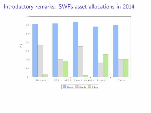
Introductory remarks: SWFs asset allocations in 2014

0

1 0

2 0

3 0

4 0

5 0

6 0

7 0

N o r w a y U A E   ­   A D I A S a u d i   A r a b i a K u w a i t Q a t a r

Equity Bonds O ther

(%)

Paper�s objectiveOur objective is to determine the optimal asset allocation for a SWFbased on income from oil. The main issues are:

I Investment horizon.I Utility function (risk aversion and time preference).I Nature of the available investment opportunity.I Oil income subject to random shocks and correlated with risky asset.

The questions of interest:

I Should �nancial assets (e.g. equity or bonds) be used to hedgeagainst oil shocks?

I Should oil be considered as an asset in the optimal allocationproblem? In other words, should we consider the optimal tradeo¤between above ground and underground wealth?

I What happens if risk aversion and the elasticity of intertemporalsubstitution change?

I What happens if the return dynamics for existing �nancial assetschange?

Related literature

Our paper draws on the following strands of the literature:

I Optimal asset allocation for a SWF:I Gintschel & Scherer (2008); Scherer (2011); van den Bremer, vander Ploeg & Wills (2016).

I Asset allocation given a stochastic stream of income:I Bodie, Merton & Samuelson (1992); Koo (1995, 1998): Veceira(2001).

I Asset allocation in the presence of state variables:I Campbell and Veceira (1999); Campbell, Chan and Veceira (2003).

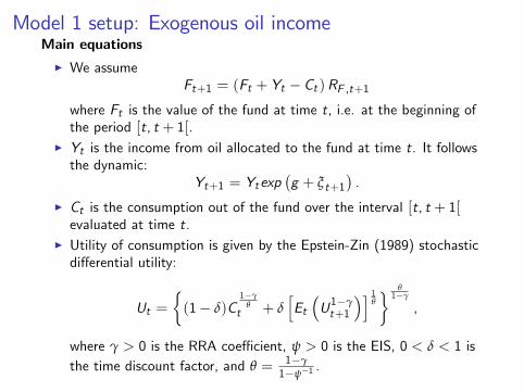
Model 1 setup: Exogenous oil incomeMain equationsI We assume

Ft+1 = (Ft + Yt � Ct )RF ,t+1where Ft is the value of the fund at time t, i.e. at the beginning ofthe period [t, t + 1[.

I Yt is the income from oil allocated to the fund at time t. It followsthe dynamic:

Yt+1 = Ytexp�g + ξt+1

�.

I Ct is the consumption out of the fund over the interval [t, t + 1[evaluated at time t.

I Utility of consumption is given by the Epstein-Zin (1989) stochasticdi¤erential utility:

Ut =�(1� δ)C

1�γθ

t + δhEt�U1�γt+1

�i 1θ

� θ1�γ

,

where γ > 0 is the RRA coe¢ cient, ψ > 0 is the EIS, 0 < δ < 1 isthe time discount factor, and θ = 1�γ

1�ψ�1.

Model 1 setup: Exogenous oil income

Financial Market Assumptions

I RF ,t = π0R0,t + π0Rt is the continuously compounded return on

the fund.I Time-varying investment opportunities: zt+1 = Φ0 +Φ1zt + νt+1,where

zt+1 =

0@ r0,t+1xt+1st+1

1A , xt+1 =

0BBB@r1,t+1 � r0,t+1r2,t+1 � r0,t+1

...rn,t+1 � r0,t+1

1CCCA .I The shocks νt+1 and ξt+1 are correlated through the vector β:

ξt+1 = β0νt+1 + σ(o)ξ

(o)t+1,

and ξ(o)t+1 is the own oil shock.

Model 1 setup: Exogenous oil income

The objective of the fund manager is to maximize the expected presentvalue of future consumption at discount rate δ:

maxfCt ,πtgE

"∞

∑t=0

δtU(Ct )

#,

subject to the intertemporal budget constraint:

Ft+1 = (Ft + Yt � Ct )RF ,t .

Model 1 setup: Exogenous oil income

Under the log-linear approximation, the optimal log consumption andportfolio composition are (lower case variables are in logs):

ct � yt = a+ b(ft � yt ) + B01zt + z

0tB2zt ,

πt = A0 + A1zt .

While the optimal allocation is linear in the state vector, the optimalconsumption path is quadratic.Focusing on the optimal allocation coe¢ cients, we have:

A0 =1

1� θ + bθψ

Σ�1xx

�HxΦ0 +

12

σ2x + σ0x �θ(1� b)

ψHx β

0Σν �

θ

ψΛ0

�� σ0x ,

A1 =1

1� θ + bθψ

Σ�1xx

�HxΦ1 �

θ

ψΛ1

�.

Model 1 setup: Exogenous oil income

Let κ = 11�θ+ bθ

ψ

Σ�1xx , the optimal allocation coe¢ cients can be

decomposed as follows:

A0|{z}Total demand

= κ

�HxΦ0 +

12

σ2x + σ0x

�� σ0x| {z }

Speculative demand

+ κ

�� θ

ψΛ0

�| {z }

Hedging demand

+κ

�� θ(1� b)

ψHx β

0Σν

�| {z }

Hedging oil shocks

,

A1|{z}Total demand

= κ [HxΦ1 ]| {z }Speculative demand

+ κ

�� θ

ψΛ1

�| {z }

Hedging demand

Model 2 setup: Oil as an asset in optimal allocation

Main equations

I We assume total wealth Wt = W ot +W

ft , where W

ot is oil wealth

and W ft represent �nancial assets.

I Ct is the consumption out of the fund over the interval [t, t + 1[evaluated at time t.

I Total wealth evolves according to

Wt+1 = (Wt � Ct )RW ,t+1.

I Utility of consumption is given by the Epstein-Zin (1989) stochasticdi¤erential utility:

Ut =�(1� δ)C

1�γθ

t + δhEt�U1�γt+1

�i 1θ

� θ1�γ

.

Model 2 setup: Oil as an asset in optimal allocationFinancial Market Assumptions

I De�ne ηt =W ot

Wtas the relative weight of oil wealth in total wealth.

I Let RW ,t+1 be the return on total wealth over the period [t, t + 1[given by

RW ,t+1 = ηt

∆W o

t+1W ot+1

!+ (1� ηt )

∆W f

t+1

W ft+1

!

= Ro ,t+1 +n

∑i=1(1� ηt )αi ,t (Ri ,t+1 � Ro ,t+1) .

I Time-varying investment opportunities: zt+1 = Φ0 +Φ1zt + νt+1,where

zt+1 =

0@ ro ,t+1xt+1st+1

1A , xt+1 =

0BBB@r1,t+1 � ro ,t+1r2,t+1 � ro ,t+1

...rn,t+1 � ro ,t+1

1CCCA .

Model 2 setup: Oil as an asset in optimal allocation

Under the log-linear approximation, the optimal log consumption andportfolio composition are (lower case variables are in logs):

ct � wt = b0 + B01zt + z

0tB2zt ,

πt = A0 + A1zt .

Considering the parameters of the optimal allocation, we have

A0 =1γ

Σ�1xx

�HxΦ0 +

12

σ2x + (1� γ)σox

�+

�1� 1

γ

�Σ�1xx

�Λ01� ψ

�,

A1 =1γ

Σ�1xx HxΦ1 +�1� 1

γ

�Σ�1xx

�Λ11� ψ

�,

Model 2 setup: Oil as an asset in optimal allocationI The total value of accumulated wealth and the optimal consumptionat time t is given by

Ct = Wtexp�b0 + B

01zt�1 + z

0t�1B2zt�1

�,

and the total wealth is updated using the budget constraint

Wt+1 = (Wt � Ct )RW ,t+1.

I The optimal solution provides the values of πt and the weight of theoptimal oil wealth is given by

1� ηt =n

∑i=1

πi ,t .

I Then we obtain the optimal oil wealth at time t + 1

W ot+1 = ηtWt+1.

I We can also �nd optimal oil reserves if we divide W ot+1 by the

expected price of oil at time t + 1.

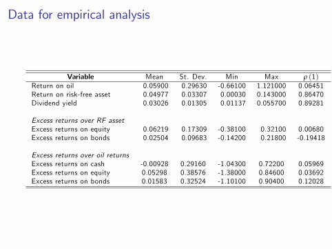
Data for empirical analysis

Variable Mean St. Dev. Min Max ρ (1)Return on oil 0.05900 0.29630 -0.66100 1.121000 0.06451Return on risk-free asset 0.04977 0.03307 0.00030 0.143000 0.86470Dividend yield 0.03026 0.01305 0.01137 0.055700 0.89281

Excess returns over RF assetExcess returns on equity 0.06219 0.17309 -0.38100 0.32100 0.00680Excess returns on bonds 0.02504 0.09683 -0.14200 0.21800 -0.19418

Excess returns over oil returnsExcess returns on cash -0.00928 0.29160 -1.04300 0.72200 0.05969Excess returns on equity 0.05298 0.38576 -1.38000 0.84600 0.03692Excess returns on bonds 0.01583 0.32524 -1.10100 0.90400 0.12028

Model 1: VAR speci�cation

The VAR(1) model is

zt+1 = Φ0 +Φ1zt + νt+1, νt+1 jFt � N (0,Σν)

where

zt =

0BB@rrf ,tereq,terbn,tdt

1CCA =

0BB@rrf ,t

req,t � rrf ,trbn,t � rrf ,t

dt

1CCA .

Model 1: VAR estimates

Dep. Var. rrf ,t+1 ereq,t+1 erbn,t+1 dt+1VAR estimation resultsConstant -0.0018 -0.0197 0.0825 0.0024

(-0.330) (-0.272) (2.084) (0.950)rrf ,t 0.7670 -2.1405 1.0284 0.0075

(8.584) (-1.828) (1.606) (0.184)ereq,t 0.0232 0.0640 -0.0092 0.0043(2.010) (0.422) (-0.111) (0.810)erbn,t -0.0741 0.1556 -0.2274 -0.0062(-3.652) (0.586) (-1.565) (-0.670)

dt 0.4163 6.1452 -3.2927 0.8951(1.813) (2.042) (-2.001) (8.550)

R 2 0.86 0.10 0.13 0.81Residual cross-correlations

rrf ,t ereq,t erbn,t dtrrf ,t 0.00017ereq,t -0.22853 0.02924erbn,t -0.58191 0.10589 0.00874dt 0.37320 -0.89851 -0.18598 0.00004

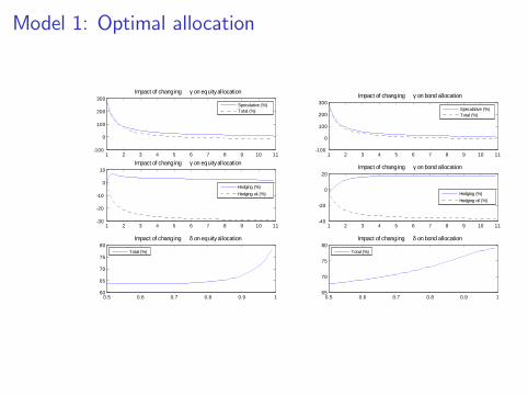
Model 1: Optimal allocation

1 2 3 4 5 6 7 8 9 10 11­100

0

100

200

300Impact of changing γ on equity allocation

1 2 3 4 5 6 7 8 9 10 11­30

­20

­10

0

10Impact of changing γ on equity allocation

0.5 0.6 0.7 0.8 0.9 160

65

70

75

80Impact of changing δ on equity allocation

1 2 3 4 5 6 7 8 9 10 11­100

0

100

200

300Impact of changing γ on bond allocation

1 2 3 4 5 6 7 8 9 10 11­40

­20

0

20Impact of changing γ on bond allocation

0.5 0.6 0.7 0.8 0.9 165

70

75

80Impact of changing δ on bond allocation

Speculative (%)Total (%)

Hedging (%)Hedging oil (%)

Total (%)

Speculative (%)Total (%)

Hedging (%)Hedging oil (%)

Total (%)

Model 2: VAR speci�cation

The VAR(1) model is

zt+1 = Φ0 +Φ1zt + νt+1, νt+1 jFt � N (0,Σν)

where

zt =

0BBBB@roil ,tbreq,tbrbn,tbrrf ,tdt

1CCCCA =

0BBBB@roil ,t

req,t � roil ,trbn,t � roil ,trrf ,t � roil ,t

dt

1CCCCA .

Model 2: VAR estimates

Dep. Var. roil ,t+1 breq,t+1 brbn,t+1 brrf ,t+1 dt+1VAR estimation resultsConstant 0.1591 -0.1839 -0.0738 -0.1611 0.0027

(1.234) (-1.096) (-0.505) (-1.267) (1.035)roil ,t 0.8182 -2.1715 0.9236 -0.0500 0.0062

(0.399) (-0.813) (0.397) (-0.025) (0.152)breq,t -0.0942 0.1976 0.0849 0.1185 0.0029(-0.328) (0.528) (0.261) (0.418) (0.508)brbn,t -0.9992 1.0966 0.6737 0.9264 -0.0076(-2.080) (1.753) (1.237) (1.954) (-0.794)brrf ,t 1.9302 -3.5124 0.1877 -1.1141 0.0132(0.898) (-1.255) (0.077) (-0.526) (0.307)

dt -3.5381 10.1057 0.7041 3.9551 0.8941(-0.671) (1.471) (0.118) (0.760) (8.486)

R 2 0.11 0.11 0.05 0.10 0.82Residual cross-correlations

roil ,t breq,t brbn,t brrf ,t dtroil ,t 0.09006breq,t -0.91137 0.15274brbn,t -0.97066 0.87736 0.11574brrf ,t -0.99910 0.90954 0.96566 0.08766dt 0.46411 -0.74165 -0.45016 -0.45341 0.00004

Model 2: Optimal allocation

2 4 6 8 10

100

200

300

Impact of changing γ on equity allocation

Myopic (%)Total (%)

2 4 6 8 10

0

10

20

Impact of changing γ on equity allocation

Hedging (%)

0.5 0.6 0.7 0.8 0.940

60

80

100Impact of changing δ on equity allocation

Total (%)

2 4 6 8 10

100

200

300

400

Impact of changing γ on bond allocation

Myopic (%)Total (%)

2 4 6 8 100

5

10

15

20

Impact of changing γ on bond allocation

Hedging (%)

0.5 0.6 0.7 0.8 0.9

60

70

80

Impact of changing δ on bond allocation

Total (%)

2 4 6 8 10

50

100

150

200Impact of changing γ on oil allocation

Myopic (%)Total (%)

2 4 6 8 10

0

1

2

Impact of changing γ on oil allocation

Hedging (%)

0.5 0.6 0.7 0.8 0.918

19

20

Impact of changing δ on oil allocation

Total (%)

Models 1 and 2: Historical allocation

1975 1980 1985 1990 1995 2000 2005 2010 2015

0

100

200

Equity and bond allocation (oil exogenous)

Equity (%)Bond (%)

1975 1980 1985 1990 1995 2000 2005 2010 2015

0

200

400

600

Equity and bond allocation (oil endogenous)

Equity (%)Bond (%)

1975 1980 1985 1990 1995 2000 2005 2010 2015

0

50

100

150

Myopic and hedging demand for equity (oil exogenous)

Myopic (%)Hedging (%)

1975 1980 1985 1990 1995 2000 2005 2010 2015

0

100

200

300Myopic and hedging demand for equity (oil endogenous)

Myopic (%)Hedging (%)

1975 1980 1985 1990 1995 2000 2005 2010 2015

0

100

200

300Myopic and hedging demand for bonds (oil exogenous)

Myopic (%)Hedging (%)

1975 1980 1985 1990 1995 2000 2005 2010 20150

200

400

600

Myopic and hedging demand for bonds (oil endogenous)

Myopic (%)Hedging (%)

Model 2: Medium-term allocation projections

Asset class 2016 2017 2018 2019 2020Equity 89.342 83.678 76.678 72.374 69.505Bonds 38.460 67.341 69.459 76.519 78.908Oil 18.853 25.514 22.683 22.773 22.076T-bills -46.655 -76.532 -68.820 -71.666 -70.489

Model 2: Long-term projections for consumption, fundvalue and oil extraction

2015 2020 2025 2030 2035 2040 2045 20500

500

1000

1500Evolution of the total wealth

2015 2020 2025 2030 2035 2040 2045 20500

50

100

150

200

250

300Evolution of oil wealth

2015 2020 2025 2030 2035 2040 2045 20500

1

2

3

4Evolution of the oil reserves

2015 2020 2025 2030 2035 2040 2045 20500

20

40

60

80

100

120Evolution of the consumption

Concluding remarks

I The objective of the paper is to study the optimal asset allocationfor an oil-based SWF:

I First: The case where oil revenue is given as an exogenous stochasticstream of income.

I Second: The case where oil is considered as an asset in the optimalallocation problem.

I The �rst model allows us to decompose the demand components asspeculative demand, hedging demand, and hedging-against-oildemand.

I The second model given myopic and hedging demand components.I The historical allocation from both models provides surprisinglysimilar results, especially with regard to allocation tradeo¤ betweenequity and bonds.

I The model�s medium-term projections indicate a need to reduceexposure to equity in favor of bonds.