optimal priority assignment and feasibility of static priority tasks with arbitrary start times

OPTIMAL PRIORITY ASSIGNMENT AND FEASIBILITYOF STATIC PRIORITY TASKS WITH ARBITRARY START TIMES

N. C. Audsley

November 1991

Real-Time Systems Research Group,Dept. of Computer Science,

University of York,York.

Y01 5DDENGLAND

ABSTRACT

Within the hard real-time community, static priority pre-emptive scheduling isreceiving increased attention. Current optimal priority assignment schemesrequire that at some point in the system lifetime all tasks must be releasedsimultaneously. Two main optimal priority assignment schemes have beenproposed: rate-monotonic, where task period equals deadline, and deadline-monotonic where task deadline maybe less than period. When tasks arepermitted to have arbitrary start times, a common release time between all tasksin a task set may not occur. In this eventuality, both rate-monotonic anddeadline-monotonic priority assignments cease to be optimal. This paperpresents an method of determining if the tasks with arbitrary release times willever share a common release time. This has complexity O(m loge m) in thelongest task period. Also, an optimal priority assignment method is given, ofcomplexity O(n 2 + n) in the number of tasks. Finally, an efficient feasibilitytest is presented, for those task sets whose tasks do not share a common releasetime.

1. INTRODUCTION

Recently, scheduling theory has enjoyed renewed interest within the real-time computingcommunity. In particular, the problem of scheduling hard real-time systems, wheremissing a single task deadline can have disastrous consequences, has motivated arenaissance of static priority pre-emptive scheduling for periodic task sets. Within thisdiscipline, for every periodic release of each task, sufficient processor resource must beguaranteed to be assigned to a task for it to meet its computational requirement before itsdeadline.

Much work has been carried out in this area to provide optimal priority assignment totasks and to check the feasibility of a task set [Liu73, Leh89, Leu80, Leu82]. Much of thiswork has used a task model which constrains all tasks to have a simultaneous release timeor critical instant [Liu73]. This simplifies both priority assignment and determination offeasibility. The main focus of this paper is to remove this constraint and to permit periodictasks to have arbitrary start times. Under these conditions, known priority assignmentstrategies are, in general, no longer optimal, with known feasibility tests either inefficientor of limited use.

The relaxation towards arbitrary start times for tasks raises a number of key issues:

(i) determining whether tasks with arbitrary start times are ever, within the systemlifetime, released simultaneously;

(ii) provision of an optimal priority assignment mechanism;

(iii) determining, in a sufficient and necessary manner, feasibility of a task set witharbitrary start times.

Formally, for a task set of cardinality n, Δ = {τ1, τ2, ..., τi, ... τn}, each task τi isassigned priority i (where 1 is the highest priority and n the lowest). Those tasks that haveyet to be assigned priority have upper case subscripts, i.e. τA, τB .. etc. Each τi has periodT i , deadline D i , computation time Ci and offset O i . The latter represents the time atwhich the first request for τi occurs, assuming that the system commences execution attime 0. Each τi makes an initial request, or release, at O i , and then periodically every T itime units. For all task deadlines to be guaranteed, for each request of a τi at t, theprocessor must be allocated to τi for Ci units in [t , t + D i), where the interval iscomposed of the D i discrete time units t, t + 1, ..., t + D i − 1.

Within this general model, we make a number of assumptions:

(i) at any point in time, the highest priority runnable task is allocated the processor;

(ii) the cost of pre-emption is zero;

(iii) pre-emptions occur at the boundaries between discrete time units;

(iv) all tasks are independent: requests for any τi are not dependent upon the initiation orcompletion of any other task;

(v) the computation requirement Ci of task τi is constant for each release;

(vi) tasks cannot be blocked;

(vii) tasks cannot voluntarily suspend themselves.

Major contributions in static priority scheduling theory for single processor systemsadhering to this model stem from the seminal paper by Liu and Layland [Liu73] describingthe rate-monotonic priority assignment for use with a simple execution model: pre-emptivestatic priority. Rate-monotonic priority assignment is optimal (amongst all possibleassignments) for periodic task sets where each τi has O i = 0 and Ci ≤ D i = T i .Priorities are assigned inversely proportional to period, i.e. the highest priority is assigned

to the shortest period task. This assignment is of O(n log2 n), i.e. that of ordering the tasksin Δ by period.

Leung et al [Leu82] describe the deadline monotonic priority assignment for task setswhere each τi has Ci ≤ D i ≤ T i . Again, this priority assignment is optimal, assuming allO i = 0. Priorities are assigned inversely proportional to deadline, with the shortestdeadline task given the highest priority. Deadline-monotonic priority assignment isequivalent to rate-monotonic when all τi ∈ Δ have T i = D i .

The problem of determining the feasibility (also termed schedulability) of a task setunder a given priority assignment is well studied. For rate-monotonic priority assignmentLiu and Layland presented a simple task set utilisation threshold test which is sufficientand not necessary [Liu73]. Hence task sets declared infeasible by the test may at runtimeprove feasible. Sufficient and necessary tests, proposed by Joseph et al [Jos86] andLehoczky et al [Leh89] are also available.

For deadline-monotonic priority assignment, Leung et al propose a feasibility testbased upon construction of a schedule until the longest deadline amongst all tasks in Δ. Ifall deadlines are met in the finite schedule, deadlines will always be met. Other feasibilitytests include those by Lehoczky [Leh90], Audsley et al [Aud90, Aud91b] and Nassor et al[Nas91]. These tests assume all tasks are initially released simultaneously (at time 0) andexamine the first deadline of each task. If this deadline is met, all subsequent deadlines forthat task will be met, since the computation demand by other higher priority tasks is at amaximum @footnote cinote@.

When the O i = 0 constraint is lifted, and the tasks in Δ never have a simultaneousrelease at runtime, the rate-monotonic priority assignment is no longer optimal. Forexample, consider tasks with equal periods. Rate-monotonic priority assignment dictatesthat the assignment of priorities of such tasks is arbitrary [Liu73]. Consider the priorityassignment of the tasks defined in example @example rate@.

Example @example rate@:

τ A : O A = 0 ; CA = 3 ; D A = 8 ; TA = 8

τ B : O B = 10 ; CB = 1 ; D B = 12 ; TB = 12

τ C : O C = 0 ; CC = 6 ; D C = 12 ; TC = 12

�Task τA is given the highest priority. The assignment of priorities for τB and τC cannot beperformed in an arbitrary manner. If τB is assigned a higher priority than τC, at time 12 τCmisses a deadline. However, if τC is assigned higher priority than τB, all tasks meet theirdeadlines. No general rule regarding the assignment of priorities to tasks with equalperiods has been identified in the literature.

If tasks are permitted arbitrary start times, with no simultaneous release of all tasksever occurring at runtime, deadline-monotonic priority assignment is also no longeroptimal. For example, consider the task set in example @example dead@.

��@footnote cinote@. The simultaneous release of all tasks can occur at any time in the systems life-time, not necessarily at time 0.

Example @example dead@:

τ A : O A = 2 ; CA = 2 ; D A = 3 ; TA = 4

τ B : O B = 0 ; CB = 3 ; D B = 4 ; TB = 8

�Deadline-monotonic priority ordering dictates that τA is assigned a higher priority than τB.However this leads to the deadline of τB being missed at time 4 (then successively at 12,20, 28 ...). When priorities are reversed, (contrary to deadline-monotonic priorityassignment) task deadlines are met. Indeed, according to Leung, who describes tasks witharbitrary offsets as asynchronous [Leu82]:

"At the present time no priority assignment has been found which is optimal foran arbitrary asynchronous system."

When considering the feasibility for tasks with arbitrary start times and nosimultaneous release, Lehoczky’s [Leh90] and Audsley’s tests [Aud91b], developed fordeadline-monotonic priority assignments, are in general, no longer necessary@footnote

intro@. For both tests, we can assume, for the purposes of determining feasibility, that allO i = 0 forcing a simultaneous release onto the task set. This creates a maximumcomputation demand on the processor producing the hardest scenario for the tasks to meettheir deadlines. Of course, at runtime a simultaneous release does not occur. Hence, byassuming all O i = 0 the feasibility tests become sufficient and not necessary.

Leung’s test, that of construction of a schedule, has been extended to cope witharbitrary task start times [Leu82]: a task set is feasible if all deadlines are met in [s , 2P)(where s = max { O 1 , O 2 , . . . , O n } and P = lcm { T 1 , T 2 , . . . , T i } ) @footnote

lcm@. The feasibility task consists of constructing a schedule for this interval. In practice,this requires the construction of a schedule for the interval [0, 2P). This approach issufficient and necessary but can be inefficient.

Clearly, an optimal priority assignment and an efficient sufficient and necessary testfor periodic task sets with arbitrary start times remain open issues. This paper focuses onthese issues, proposing an integrated approach to priority assignment and schedulability.This is in contrast to previous work cited above, which separately addresses the issues ofpriority assignment and feasibility testing. The integrated approach uses feasibility testingas part of task priority assignment. Thus, when a valid priority assignment is found, thetask set is known to be feasible. Additionally, the problem of determining if all tasks in atask set will ever have a common release time is addressed.

The remainder of this paper is arranged as follows. The next section provides amethod for determining if and when tasks share a common release time. Section 3discusses optimal priority assignment. Section 4 defines a minimum interval that must beconsidered when determining the feasibility of a task. Section 5 proposes a sufficient andnecessary test that combines priority assignment and feasibility to provide an integratedapproach. Concluding remarks are offered in section 6.

��@footnote intro@. Both these tests are applicable to any fixed priority assignment rule. They arenot limited to task priorities assigned by the deadline-monotonic method.@footnote lcm@. lcm - least common multiple of a set of integers.

2. CRITICAL INSTANTS

The feasibility tests for static priority periodic task systems cited in section 1 are foundedon the assumption that at some point of time during the lifetime of the system all tasksshare a common release time. This is termed the critical instant [Liu73] @footnote

criticalinstant@. When a critical instant occurs, the worst-case load on the processorbecomes apparent. In a static priority pre-emptive system, this forms the hardest time forall task deadlines to be guaranteed: Theorem 1 in [Liu73] shows that if deadlines can beguaranteed for releases starting at a critical instant, they can be guaranteed, by implication,for the lifetime of the system.

When tasks have offsets, it is difficult, by inspection of task timing characteristicsalone, to determine if a critical instant will occur during system execution. If a criticalinstant does not exist, different priority assignments and feasibility tests need to beemployed for optimality to be achieved.

The following discussion details how to determine if a task set contains a criticalinstant. Firstly, we constrain the problem to that of determining if two tasks share acommon release time. This result is developed in the subsequent section to show how todecide if a task set of arbitrary cardinality has a critical instant.

2.1. Two-Tasks

Consider Δ = {τ1, τ2}. We note that for any τi ∈ Δ, without loss of generality, ifO i = T i , O i can be set to 0. If O i > T i , we can reduce the offset to be O i − � O i /T i � T i .Hence, we can state that O 1 < T 1 and O 2 < T 2. Thus, a critical instant will occur if

O 1 + aT1 = O 2 + bT2 [a,b ∈ Z]

Without loss of generality, we can reduce the smallest offset to be 0. Let O 1 < O 2. Thusthe critical instant condition becomes:

riticalInstantCondition@)’aT1 = O2′ + bT2 [a,b ∈ Z ; O2

′ = O 2 − O 1 ](@equation

This is a linear diophantine equation in two variables. Equation (@equationCriticalInstantCondition@) holds if and only if the greatest common divisor (gcd) of T 1and T 2 divides exactly into O2

′ [Jac75]. Thus, a critical instant exists if and only if

CDcondition@)’O2′ = h gcd(T 1 , T 2 ) [h ∈ Z] (@equation

We note that the gcd can be found using Euclid’s Algorithm (algorithm 1.1.E in [Knu73] ).This has complexity O(loge max{T 1 , T 2 }).

Consider the task set given in example @example twotasksci@.

Example @example twotasksci@:

τ A : O A = 3 ; TA = 42

τ B : O B = 66 ; TB = 147

�We let O A ′ = 0 and O B ′ = 63. Since gcd(42, 147) = 21 and O B ′ = 3×21, a commonrelease time exists between the tasks. Indeed, releases of τA occur at 0, 42, 84, 126, 168,210,.. Releases of τB occur at 63, 210,.. Common release times are 210, 594, 798,...��@footnote criticalinstant@. A critical instant refers to a simultaneous release of all tasks in Δ. Asimultaneous release of a subset of tasks in Δ is termed a common release time.

2.2. Many Tasks

We extend the problem to Δ = {τ1, τ2 ... τn}. Two approachs are identified.

Naive Approach

Compare every release of τi (1 ≤ i ≤ n) with every τj (j = 1 to i − 1, i + 1 to n). Thisrequires a total number of comparisons given by:

cre@)’i = 1Σn

j = i + 1Σn �

�� T i

lcm(T i , T j )��

(@equation

In the worst case lcm(T i ,T j ) = T i T j , giving:

�� T i

lcm(T i , T j )��

=�� T i

T i T j��

= T j

Therefore, equation (@equation wcre@) can be restated:

i = 1Σn

j = i + 1Σn

T j =i = 2Σn

( i − 1) T i

The complexity of this approach is O(i = 2Σn

( i − 1) T i). Hence, in general the approach is

exponential.

Efficient Approach

We use the results of section 2.1 to establish a more efficient approach. Consider twotasks, τA and τB, that share a critical instant (i.e. use the method in section 2.1). Assumethat O A = 0 and 0 < O B < TB . We can form a hybrid task, τAB to represent the criticalinstant of the two tasks throughout the system lifetime. The period of τAB will be the timebetween successive critical instants, with O AB being the time from 0 to the first criticalinstant (hence O AB ≥ O B). Thus we replace two tasks with one.

We now identify the period and offset of τAB. The period, TAB , is the lcm of TA andTB

@footnote lcmgcd@:

itab@)’TAB =gcd(TA , TB )

TA TB�� (@equation

Since the denominator has already been found (when determining if a critical instant existsbetween τA and τB) the calculation of TAB is trivial.

The offset can be calculated using the Euclidean algorithm for finding the gcd of twointegers. This can be adapted to find two integers x and y such that (algorithm 1.2.1.Ein[Knu73] ):

xTA + yTB = gcd(TA , TB )

We note that x and y represent one of an infinite set of solutions for this expression.Multiplying through by h:��@footnote lcmgcd@. The lcm of two integers a, b, is related to the gcd of a, b, byab/gcd(a,b) = lcm(a,b). For further details see theorem 2.5 in [Ros85].

(hx) TA + (hy) TB = h gcd(TA , TB )

Since by equation (@equation GCDcondition@) OB = h gcd(TA , TB ):

uclidone@)’(hx) TA + (hy) TB = OB (@equation

We note that one of x and y will be negative, the other positive. If the multiplier of TA isnegative, we have effectively extrapolated a common release time of the tasks prior to time0. To find a common release time after 0 we need to make the multiplier of TA positive andthat of TB negative. This is achieved by noting that common release times occur withperiod TAB. Thus, we add kTAB to the first term of equation (@equation Euclidone@)subtract the same quantity from the second term:

uclidtwo@)’(hxTA + kTAB ) + (hyTB − kTAB ) = OB (@equation

where

uclidk@)’k =�� TAB

| x| hTA��

(@equation

Since the first term of equation (@equation Euclidtwo@) is positive and the secondnegative, we may rearrange:

uclidFinal@)’(hx) TA + kTAB = (hy) TB + kTAB + OB (@equation

Either side of equation (@equation EuclidFinal@) defines a simultaneous release of τA andτB after 0. Let t equate to one side of equation (@equation EuclidFinal@):

uclidt@)’t = (hx) TA + kTAB (@equation

It may occur that t > TAB or that t > lcm(TA , TB ). Therefore we form OAB by subtractingfrom t a multiple of lcm(TA , TB ), the resulting quantity representing the first release of τAB,that is OAB:

askaboffset@)’OAB = t −�� TAB

t��TAB (@equation

where k and t are defined by equations (@equation Euclidk@) and (@equation Euclidt@)respectively. We note that OAB ≥ OB as TAB ≥ TB and OB < TB.

We have shown that if two tasks τA and τB have a critical instant, we can form thehybrid task τAB with period TAB and offset OAB (given by equations (@equation citab@)and (@equation taskaboffset@) respectively). τAB defines the common release times of τAand τB.

Successively, we can apply this technique to the remaining tasks in Δ: we compareτAB and τC ∈ Δ − {τA, τB}. If these two tasks share a critical instant (by section 2.1), weformulate τABC. Therefore, we can determine whether the tasks in Δ share a critical instant.If this is so, the resulting hybrid task, by its offset and period, will characterise thecommon release times of the tasks in Δ.

The complexity of this method is now considered. For each combination of two tasks(or one hybrid and one task) the cost involves:

(i) deciding whether a critical instant exists for the two tasks;

(ii) formulating the hybrid task: this is trivial by equations (@equation citab@) and(@equation taskaboffset@).

Since we may create a maximum of n − 1 hybrid tasks for a task set containing n tasks, thecomplexity of finding if the tasks in Δ share a critical instant is, as n→∞,

O(n loge max{TA ,TB ,TC ,..}). This is clearly more efficient (and less exponential) than the"Naive Approach".

We return to example @example twotasksci@ noting that OA = 0 and OB = 63. Insection 2.1 it was shown that the tasks had a common release time. By evaluation of theschedule the first such time is 210. We now derive the hybrid task τAB. Evaluating TAB

according to equation (@equation citab@), noting that gcd(TA , TB ) = 21 :

TAB =gcd(TA , TB)

TA TB�� =21

6174�� = 294

Evaluating k in equation (@equation Euclidk@), noting that h = 3:

k =�� TAB

| x| hTA��

=�� 294

3 × 3 × 42��

= 2

Evaluating t according to equation (@equation Euclidt@):

t = (hx) TA + kTAB = ( − 9 × 42) + (2 × 294) = 210

Evaluating OAB according to equation (@equation taskaboffset@):

OAB = t −�� TAB

t��TAB = 210 −

�� 294

210��210 = 210

Thus the hybrid task has period TAB = 294 and offset OAB = 210. We note that OAB

corresponds to the first common release of τA and τB.

3. OPTIMAL PRIORITY ASSIGNMENT

In the previous section it was shown how to check if the tasks in Δ will ever be releasedsimultaneously. Tasks sets whose tasks will never undergo such a release are termed non-critical-instant tasks sets, Δ* (the set of all Δ* is a subset of the set of all Δ). For any Δ*,section 1 indicated that neither rate-monotonic or deadline-monotonic priority assignmentswere optimal. We now develop an optimal priority assignment for tasks with arbitrary starttimes.

Consider Δ* = {τA, τB, τC,...} of cardinality n. A priority assignment function mapseach task onto a different priority level. For Δ* there are n! distinct priority assignmentsover the task set, hence the set of distinct priority assignment functions has cardinality n!.This is denoted by Φ = {Φ1 , Φ2 , . . . , Φn!}. We denote the mapping of a task onto apriority level by

Φ i (τA ) = j

where the i th priority assignment function maps τA onto priority level j. The inversemapping, of priority level to task, is denoted:

Φi− 1 ( j) = τA

When the priority ordering over Δ* specified by a priority ordering function is feasible, weterm that function a feasible priority assignment function.

In general, τA is feasible (schedulable) if and only if [Aud90, Aud91b]:

CA + I A ≤ DA

where I A represents the execution requirement (interference) of higher priority tasks in the

interval defined by the release and deadline of τA.

If τA is not feasible, and the task timing characteristics cannot be changed (i.e. CA

cannot be decreased and DA cannot be increased), the only way to make τA feasible is todecrease I A. This is achieved by changing the priority ordering over Δ* by using a priorityassignment function that reduces the priority of a higher priority task to be lower than τA.(Note that we could then promote a lower priority task to be higher than τA as long as thenew I A is less than the original.)

Let us now consider the effect on the feasibility of Δ* (cardinality n) for Φ x ∈ Φ suchthat Φ x (τA ) = n. We present two theorems regarding such an assignment.

Theorem @theory prilow1@:If τA is assigned the lowest priority, n, and is infeasible, no priority assignmentfunction that assigns τA priority level n produces a feasible assignment.

Proof:Amongst the n! distinct priority assignment functions, (n − 1) ! produce anassignment with τA at priority level n. For all such assignments, the interferencedue to tasks of higher priority than τA is equal, as the same set of tasks is ofhigher priority than τA in each ordering. Thus if τA is infeasible as the lowestpriority task by one assignment function, it will be infeasible under the priorityordering of any other function assigning it the lowest priority.

�

Theorem @theory prilow2@If τA is assigned the lowest priority, n, and is feasible, then if a feasible priorityordering for Δ* exists, an ordering with τA assigned the lowest priority exists.

Proof:Let us assume that an assignment function Φ y produces the feasible assignment:

Φ y (τB ) = 1, Φ y (τC ) = 2, , . . . , Φ y (τA ) = i, Φ y (τD ) = i + 1, , . . . , Φ y (τE ) = n

We note that τA is feasible at priority level i < n. A second priority assignmentfunction Φ x defines:

Φ x (τB ) = 1, Φ x (τC ) = 2, , . . . , Φ x (τD ) = i, , . . . , Φ x (τE ) = n − 1, Φ x (τA ) = n

Since τA is feasible if assigned priority level n (by the theorem), we can assignτA to level n. The tasks originally assigned priority levels i + 1 . . . n in Φ x arepromoted 1 place (i.e. the task at priority level i + 1 is now assigned priority i).Clearly, the tasks assigned levels 1 . . . i + 1 remain feasible as nothing haschanged to affect their feasibility. The tasks originally assigned levelsi + 1 . . . n also remain feasible as the interference on them has decreased withτA now being of the lowest priority. Since τA is feasible at the lowest prioritylevel, at least one feasible priority assignment exists with τA as the lowestpriority task. The theorem is proved.

�The above theorems limit considerations to priority level n. We now extend the above twotheorems, to consider assignment of arbitrary priorities to tasks, rather than merely priorityn.

Theorem @theory inductive@:Let the tasks assigned priority levels i, i + 1,.., n by assignment function Φ x befeasible under that priority ordering. If there exists a feasible priority ordering

for Δ*, there exists a feasible priority ordering that assigns the same tasks tolevels i..n as Φ x.

Proof:We prove the theorem by showing that a feasible priority assignment functionΦ y can be transformed to assign the same tasks to priority levels i, i + 1,.., n asΦ x, whilst preserving the feasibility of Φ y. The proof is by induction: Φ y istransformed successively moving tasks Φx

− 1 (n) , Φx− 1 (n − 1) ,.., Φx

− 1 (i) to prioritylevels n, n − 1,..,i under Φ y.BaseLet Φx

− 1 (n) = τA and Φ y (τA ) = m, where m ≤ n. By theorem @theory prilow2@we can move τA to the assigned level (n) under Φ k without altering the feasibilityof Δ*.Inductive HypothesisWe assume that the tasks assigned to priority levels n − 1, n − 2, .., i + 1 under Φ x

are moved to levels n − 1, n − 2, .., i + 1 under Φ y. Δ* is assumed to remainfeasible.Inductive StepLet Φx

− 1 (i) = τB and Φ y (τB ) = m, where m ≤ i (since the reassignment of prioritylevels n, n − 1, .., i + 1 has promoted τB to have a priority of between 1 and i).Under both orderings, the tasks assigned to priority levels i + 1, .., n are identical.Task τB is reassigned in Φ y to level i. We know (by Φ x) that τB is feasible at thislevel (assuming that tasks assigned to levels i + 1..n are identical under Φ x andΦ y).After the reassignment, tasks at levels 1..i − 1 remain feasible, as their respectiveinterferences are no greater than before the reassignment and therefore mustremain feasible. This proves the theorem.

�We now use the above theorems in developing an optimal static priority assignment

scheme which assigns tasks to priority levels n, n − 1,.., 1 in order. Only if a feasibleassignment can be made to priority level i do we proceed to priority level i − 1. A genericapproach for assigning to level i (1 < i ≤ n) is now given.

Task Assignment to Priority Level i

We assume that priority levels n..i + 1 have been assigned such that the tasks assigned tothose levels are feasible. Let the task assigned to priority level j be given by Ψ( j). We notethat Ψ( j) is only defined for i < j ≤ n. Let the set Δi+1 be composed of those tasks in Δ*

that have been assigned priority levels n, n − 1,..,i + 1 (cardinality of Δi+1 is n − i). For eachtask τA in Δ*-Δi+1 (i.e. the set of unassigned tasks) we select a single Φ k ∈ Φ such that

∀l : i < l ≤ n : Φk− 1 (l) = Ψ(l)

The set of such Φ k for priority level i is termed Φi. Set Φi contains i elements of Φ, each ofwhich assigns priority levels n to i + 1 identically, differing in their assignment of prioritylevel i (each Φ k assigns a different τr ∈ Δ*-Δi+1 to level i).

For each Φ k ∈ Φi we check the feasibility of the task assigned priority level i (byvirtue of reaching the assignment of priority level i we know that tasks assigned to levelsn, n − 1,..,i + 1 are feasible). Two cases are identified:

(i) all tasks are infeasible when assigned priority level i;

(ii) one or more tasks are feasible when assigned priority level i.In the first case, we know by theorem @theory prilow1@ that no feasible priority

assignment exists for Δ* and so the task set is infeasible. In the second case, we mayarbitrarily select one of the feasible tasks noting by theorem @theory inductive@ that if afeasible priority assignment for Δ* exists, one will exist with the selected task assignedpriority level i. Thus, Ψ(i) is defined. We proceed to the assignment of priority level i − 1.

Eventually, we reach the assignment for level 1. This is trivial since at this stage onlone task remains to be assigned (i.e. the cardinality of Δ*-Δ2 is 1) leaving no choice forpriority level 1. The next section gives an efficient implementation for this method ofpriority assignment.

Algorithmic Implementation

An algorithm implementing the priority assignment method detailed in the previoussections is now given.

Algorithm @algorithm priassign@: Optimal Priority Assignment:

PriorityAssignment ()

begin

Δ = Δ* -- copy the non-critical instant task set

for j in (n..1) -- priority level j

unassigned = TRUE

for τA in Δif (feasible(τA, j)) then -- if τA is fesaible

-- for priority level j

ψ(j) = τA -- assign τA to priority level j

Δ = Δ - τA

unassigned = FALSE

endif

if (unassigned)

exit -- no feasible priority assignment exists

endif

endfor

endfor

end

�Firstly, we attempt to find a task τA that is feasible at priority level j = n. If one is found,then by theorem @theory prilow2@ if a feasible priority assignment function exists, onealso exists with τA assigned priority level n, i.e. Ψ( j) = τ n. Next, priority level j = n − 1 isnow considered. If a task can be found (amongst the n − 1 tasks that have not yet beenassigned a priority level) that is feasible at priority level n − 1, then by theorem @theoreminductive@ we know that if a feasible priority assignment function exists, a feasiblepriority one also exists with this task assigned priority level n − 1. Successively, tasks arefound that are feasible at priority levels n to 1. If, for any priority level j a feasible taskcannot be found, no feasible priority assignment function exists.

Discussion

This priority assignment scheme is optimal in the sense that if a feasible priority orderingexists for a task set, it will be found by this method. The proof of this assertion lies intheorems @theory prilow1@, @theory prilow2@ and @theory inductive@.

The complexity of the priority assignment scheme lies in the number of priorityassignment functions examined. This is more readily described by examining thebehaviour of algorithm @algorithm priassign@. To find a task that is feasible at prioritylevel n involves testing the feasibility of a maximum of n tasks. In general, to find a taskfeasible when assigned priority level i ≤ n requires testing the feasibility of a maximum of i

tasks (that is the i tasks that have yet to be assigned a priority). Therefore, across allpriority levels, the number of tests required, B, is given by:

B = n + (n − 1) + (n − 2) + ... + (n − (n − 2)) + (n − (n − 1))

Since there are n terms

B = n 2 − 1 − 2 − . . . − (n − 1) = n 2 − n −i = 1Σ

n − 1

i

Since the sum of all integers between 1 and m is m(m + 1)/2

B = n 2 −2

(n − 1) n�� =21�� (n 2 + n)

Therefore, finding a feasible priority assignment or showing that no such assignment existsrequires that a maximum of n 2 + n priority assignment functions be examined. In effect,the feasibility of a maximum of n 2 + n tasks needs to be determined. This is polynomial inn and as such is exponentially more efficient than examining all possible n! priorityorderings.

The priority assignment technique detailed above relies upon a sufficient andnecessary feasibility test being available. Such a test is developed in the following sections.

4. FEASIBILITY INTERVAL

Feasibility testing of a task set requires the definition of an interval over which that testingneeds to occur. We term this the feasibility interval. For tasks which share a criticalinstant, feasibility can be determined by examining the first deadline of each task after acritical instant. This approach is used in many of the feasibility tests cited in section 1 forstatic priority task sets. Hence the feasibility interval for each τi is [t, t + Di) where t

corresponds to a simultaneous release of all tasks. When arbitrary task start times arepermitted, or more specifically when the tasks form a non-critical-instant task set, thisapproach is not appropriate.

Leung et al [Leu80, Leu82, Leu89] showed that an interval of [Omax , 2P) is asufficient interval (where Omax represents the maximum process offset and P is defined bythe lcm of all task periods). This interval was established by considering dynamic priorityscheduling schemes, such as Earliest Deadline. For static priority schemes we now showthat, in general, a smaller interval is sufficient.

We make the initial observation that the feasibility of an individual task in a staticpriority pre-emptive scheduling scheme depends only upon itself and other tasks of higherpriority. Therefore, when determining the lower and upper endpoints for the feasibilityinterval of τi ∈ Δ* we consider τi and those tasks in Δ* of higher priority. Considering theoptimal priority assignment method introduced in section 3, all priority levels 1..i − 1 are

unassigned. Therefore, without loss of generality, we arbitrarily assign currentlyunassigned tasks to those levels. When determining the feasibility interval, the specificassignments of levels 1..i − 1 is not important, only that all unassigned tasks have prioritygreater than τi.

To aid the following discussion, we refine the offsets of the tasks in Δ* withoutaltering their relative phasing. The following theorem expresses this refinement.

Theorem @theory refine@:When determining the feasibility interval for τi ∈ Δ*, the timing characteristicsof tasks τ1, τ2,..., τi-1 can be rearranged, without altering the relative phasing ofthose task releases, such that:

(a) min (O1. . . Oi ) = Oi = 0

(b) ∀ τj ∈ {τ1,.. τi} : Oj ∈ [Oi , Oi + Pi)

Proof:Let the offsets of tasks τ1, τ2,.. τi be represented by (O1 , O2 , . . . , Oi ). We canform condition (a) by adding an amount l j to Oj for any task τj ∈ {τ1, τ2,.., τi-1}where Oj < Oi. To preserve the relative phasing of the tasks, l j is a multiple ofTj. Also, l j must be at least Oi − Oj. Therefore, we define

j@)’l j =�� Tj

Oi − Oj��

(@equation

Thus

l j T j ≥ Oi − Oj

Therefore we have

Oi ≤ Oj + l j T j

where l j is defined by equation (@equation lj@). Since Tj ≤ Pi and Oj < Oi,

Oi ≤ Oj + l j T j < Oi + Pi

Hence we can transform (Oi. . . Oi ) into (O1

′ O2′ . . . Oi

′ ) by the function:

Oj′ =

�� if Oi ≤ Oj

if Oi > Oj

Oj′ = Oj

Oj′ =

�� Tj

Oi − Oj��Tj + Oj

We note that the transformation of Oi (to Oi) is defined by the function, althoughnot necessary. Once transformed to meet (a), the task set also meets (b), sinceall Oj < Tj. Without loss of generality, we can now assign Omin = 0 with allother offsets reduced by Omin. We note task phasing is not affected.

�With task timing characteristics rearranged according to Theorem @theory refine@, wecan now establish the feasibility interval for τi. Firstly, we define the initial stabilisationtime at the start of the task set execution.

Definition @definition stabilisation@:The initial stabilisation time, S j, of task τj, is the time after which the executionof the task set repeats exactly every Pj with respect to tasks τ1, τ2,..., τj.�

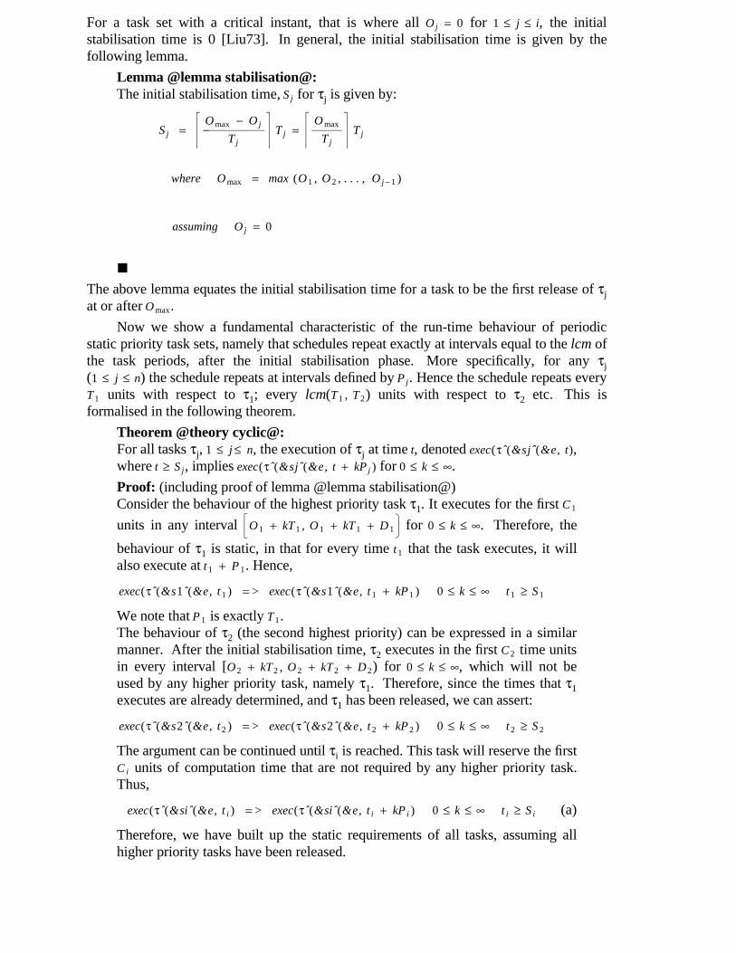
For a task set with a critical instant, that is where all Oj = 0 for 1 ≤ j ≤ i, the initialstabilisation time is 0 [Liu73]. In general, the initial stabilisation time is given by thefollowing lemma.

Lemma @lemma stabilisation@:The initial stabilisation time, S j for τj is given by:

S j =�� Tj

Omax − Oj��Tj =

�� Tj

Omax��Tj

where Omax = max (O1 , O2 , . . . , Oj − 1 )

assuming Oj = 0

�The above lemma equates the initial stabilisation time for a task to be the first release of τjat or after Omax.

Now we show a fundamental characteristic of the run-time behaviour of periodicstatic priority task sets, namely that schedules repeat exactly at intervals equal to the lcm ofthe task periods, after the initial stabilisation phase. More specifically, for any τj(1 ≤ j ≤ n) the schedule repeats at intervals defined by Pj. Hence the schedule repeats everyT 1 units with respect to τ1; every lcm(T 1 , T 2) units with respect to τ2 etc. This isformalised in the following theorem.

Theorem @theory cyclic@:For all tasks τj, 1 ≤ j ≤ n, the execution of τj at time t, denoted exec(τˆ(&sjˆ(&e, t),where t ≥ S j, implies exec(τˆ(&sjˆ(&e, t + kPj ) for 0 ≤ k ≤ ∞.

Proof: (including proof of lemma @lemma stabilisation@)Consider the behaviour of the highest priority task τ1. It executes for the first C 1

units in any interval �� O1 + kT1 , O1 + kT1 + D1

�� for 0 ≤ k ≤ ∞. Therefore, the

behaviour of τ1 is static, in that for every time t 1 that the task executes, it willalso execute at t 1 + P 1. Hence,

exec(τˆ(&s1ˆ(&e, t 1 ) = > exec(τˆ(&s1ˆ(&e, t 1 + kP 1 ) 0 ≤ k ≤ ∞ t 1 ≥ S 1

We note that P 1 is exactly T 1.The behaviour of τ2 (the second highest priority) can be expressed in a similarmanner. After the initial stabilisation time, τ2 executes in the first C 2 time unitsin every interval [O2 + kT2 , O2 + kT2 + D2) for 0 ≤ k ≤ ∞, which will not beused by any higher priority task, namely τ1. Therefore, since the times that τ1executes are already determined, and τ1 has been released, we can assert:

exec(τˆ(&s2ˆ(&e, t 2 ) = > exec(τˆ(&s2ˆ(&e, t 2 + kP 2 ) 0 ≤ k ≤ ∞ t 2 ≥ S 2

The argument can be continued until τi is reached. This task will reserve the firstCi units of computation time that are not required by any higher priority task.Thus,

exec(τˆ(&siˆ(&e, t i ) = > exec(τˆ(&siˆ(&e, t i + kPi ) 0 ≤ k ≤ ∞ t i ≥ S i (a)

Therefore, we have built up the static requirements of all tasks, assuming allhigher priority tasks have been released.

The only time that the assertion (a) does not hold is if at time t i, there exists ahigher priority task τj that has not yet been initially released, (i.e. t i < Oj). Inthis case, it may occur that exec(τˆ(&siˆ(&e, t), but that exec(τˆ(&sjˆ(&e, t i + kTi )

as t i < Oj ≤ t i + kTi. This can only occur if τj has not been released, whichcontradicts Theorem @theory cyclic@ and Lemma @lemma [email protected] Theorem @theory cyclic@ holds given Lemma @lemma stabilisation@.

We now proceed to prove Lemma @lemma [email protected] tasks are initially released before or at Omax (assuming offset refinement byTheorem @theory refine@). However, this is not a sufficient value for S i.Consider a release of τi before Omax with a deadline after Omax. That is:

Oi + nTi < Omax < Oi + nTi + Di (b)

Since τi is released before some higher priority tasks, this could lead to a time t

such that

Omax < t < Oi + nTi + Di

which is idle but with the following condition holding:

exec(τˆ(&siˆ(&e, t + mTi ) m ≥ 1

That is, due to τi running before all higher priority tasks had not been released, τicompleted its execution defined by (b) early in comparison to corresponding execu-tions in subsequent Pi periods. This cannot occur in releases of τi beginning at orafter Omax. Therefore S i corresponds to the first release of τi after Omax, given in Lem-ma @lemma [email protected], Theorem @theory cyclic@ and Lemma @lemma stabilisation@ are proved.

�Theorem @theory cyclic@ and Lemma @lemma stabilisation@ can now be restated togive the feasibility interval for τi.

Theorem @theory interval@:Task τi is feasible if and only if the deadlines corresponding to releases of thetask in [S i , S i + Pi) are met.

Proof: By Theorem @theory cyclic@ any τi ∈ c that executes at timet ∈ [S i , S i + Pi ) will also execute at t + Pi. Therefore, the schedules in thefollowing intervals will be identical (with respect to τ1, τ2,.. τi):

[S i , S i + Pi )

[S i + Pi , S i + 2Pi )

. . .

[S i + mPi , S i + (m + 1) Pi )

If a task deadline is missed at d from the beginning of one interval, it will bemissed at d from the beginning of all such intervals. Therefore it is sufficient tocheck the deadlines of one interval only, so proving Theorem @theoryinterval@.

�

Discussion

The feasibility intervals defined in the above sections are shorter than those proposed byLeung et al [Leu80, Leu82]. The latter interval is designed for testing earliest deadlinefeasibility. Therefore, determining static feasibility requires less evaluation than fordynamic in two main ways. Firstly, the latter requires twice the lcm to be examined.Secondly, dynamic feasibility requires the lcm of all task periods, whilst Theorem @theoryinterval@ only requires the lcm to consider the periods of tasks with greater or equalpriority to the task whose feasibility is being considered.

The interval derived in this section will be exponentially less than that proposed byLeung for most task sets. Consider 5 tasks with relatively co-prime periods, i.e.T 1 = 9, T 2 = 11, T 3 = 13, T 4 = 17, T 5 = 29. Under Leung’s method, each task is examinedfor twice the lcm of all periods @footnote leung@, hence the feasibility interval for each taskis 1,268,982 long, 6,344,910 in total (for the 5 tasks). The interval derived in the previoussection has total length T 1 for τ1, T 1 T 2 for τ2 etc. This evaluates to a total of

9 + (9 × 11) + (9 × 11 × 13) + (9 × 11 × 13 × 17) + (9 × 11 × 13 × 17 × 29) = 657705

This is approximately 10% of the total length of Leung’s interval. In general, the length ofeither interval is at a maximum when all task periods are co-prime. In this case, Leung’sinterval for n tasks becomes

Leung_Interval_Total = 2n(T 1 T 2 ...Tn ) (@equation

The interval derived above becomes

New_Interval_Total = T 1 + T 1 T 2 +... + T 1 T 2. . . Tn (@equation

If all task periods are unitary, we have Leung_Interval_Total = 2n and New_Interval_Total = n.Let all task periods be mutually co-prime, with Ti < Ti + 1 (1 ≤ i < n). We can state that:

Leung_Interval_Total > New_Interval_Total (@equation

Substituting (@equation leungint@) and (@equation newint@):

2n(T 1 T 2. . . Tn ) > T 1 + T 1 T 2 +... + T 1 T 2

. . . Tn

Taking T 1 T 2. . . Tn from each side:

2(n − 1)(T 1 T 2. . . Tn ) > T 1 + T 1 T 2 +... + T 1 T 2

. . . Tn − 1

The left hand side can be expanded to n − 1 terms of 2(T 1 T 2. . . Tn ), giving n − 1 terms on

each side. Comparing terms, each 2(T 1 T 2. . . Tn ) is clearly greater than corresponding

terms on the right hand side. Thus, equation (@equation compareints@) holds. Thedifference between left and right hand sides is given by:

Leung_Interval_Total − New_Interval_Total =

(2nT 2. . . Tn − 1) T 1 + (2nT 3

. . . Tn − 1) T 1 T 2 +... + (2nTn − 1) T 1 T 2. . . Tn − 1

Thus, in general, New_Interval_Total is exponentially less than Leung_Interval_Total.

��@footnote leung@. Leung’s approach incorporates the construction of a schedule over an intervalequal to twice the lcm of all task periods. In the worst case, when inserting any task into theschedule, each slot in that schedule has to be examined. Hence, each task requires a check of theentire interval.

5. FEASIBILITY AND PRIORITY ASSIGNMENT

Optimal priority assignment requires a sufficient and necessary feasibility test. Theprevious section showed that such a test need only check deadlines of τi in [S i , S i + Pi) toestablish feasibility. This section provides a method for examining feasibility and showshow the combined optimal priority assignment and feasibility approach work in practice.

5.1. Feasibility Testing

The primary result of section 4 was that feasibility of a task set can be determined byexamining the executions of each task over its feasibility interval (defined by theorem@theory interval@). This could be achieved by the construction of a schedule over eachfeasibility interval. This requires that for τ1,τ2..τi, we assign sufficient slots in a schedulefor each task to meet its deadlines. However, since we need to know exactly how muchoutstanding computation needs to be honoured at S i, the schedule has to be constructed for[0, S i + Pi). This is an increase of S i over the exact feasibility interval required. S i canhave a maximum value given by:

Simax = max1 ≤ j ≤ i {τ j } + Ti − 1

Therefore, as n increases, the additional interval length becomes less intrusive. Thisapproach is inefficient in that, in the worst case, the entire schedule has to be examined foreach task.

We now introduce a more efficient approach. For the purposes of the followingdiscussion, we assume that task offsets have been adjusted according to theorem @theoryrefine@. For a release of τi at t, we can state that it will meet its deadline if and only if thecomputational demands of higher priority tasks and Ci are no greater than Di. That is:

Iit + Ci ≤ Di (@equation

Since the feasibility of an individual task in a static priority pre-emptive schedulingscheme depends only upon itself and other tasks of higher priority, when determining thefeasibility interval of τi ∈ Δ* we consider τi and those tasks in Δ* of higher priority.Considering the optimal priority assignment method introduced in section 3, all prioritylevels 1..i − 1 are unassigned. Therefore, without loss of generality, we arbitrarily assigncurrently unassigned tasks to those levels. When determining feasibility, the specificassignments of levels 1..i − 1 is not important, only that all unassigned tasks have prioritygreater than τi.

The term Iit is defined as follows:

Definition @definition interference@:

The interference that is suffered by τi due to higher priority tasks wishing toexecute during the release of τi starting at t is defined as Ii

t.

�The interference Ii

t is made up of two parts: the execution demands of higher priority tasksthat have been released before t and have deadlines after t; and the executions of higherpriority tasks released in [t, t + Di). We now define these two terms.

Definition @definition remaining@:

The remaining interference on a release of τi at time t, due to higher prioritytasks that have not completed their execution at t, is defined as Ri

t.

�

Definition @definition created@:

The created interference on a release of τi at time t, due to higher priority tasksreleased in the interval [t, t + Di), is defined as Ki

t.

�Formally, we can state that the interference on τi during the release starting at t is

Iit = Ri

t + Kit

Hence, at each release of τi at t, if the following condition holds, τi is feasible for thatrelease.

Rit + Ki

t + Ci ≤ Di

Formally, for the entire task set, the feasibility condition becomes:

∀i : 1 ≤ i ≤ n (@equation

∀t ∈ Bi : Rit + Ki

t + Ci ≤ Di

B i =�t | t ∈ (S i , S i + Ti , S i + 2Ti ,....,S i + Pi )

� �

Any test based upon the feasibility intervals defined by theorem @theory interval@ usingthe feasibility condition given by equation (@equation feasible@) will be sufficient andnecessary if and only if the values of Ri

t and Kit are exact.

We now move to define Rit and Ki

t together with a sufficient and necessary feasibilitytest.

Exact Calculation of Rit

The easiest method for determining Rit is to construct and examine a schedule for the

interval [0, t), for each release of τi at t. This is clearly inefficient. A better solution wouldbe to adopt Leung’s approach [Leu80], and construct a schedule for the entire task set forthe interval [0, tmax), where tmax is defined by the maximum endpoint of the n feasibilityintervals defined for the tasks in Δ*. This again is inefficient.

Another approach can be derived by noting, when we consider the feasibility of τi,that its first release occurs at time 0 @footnote exact@. Therefore, since the interference dueto higher priority tasks released at time 0 will be included in Kt

i, we have Ri0 = 0.

Definition @definition lit@:

Lit represents the outstanding computation requirement by tasks τ1..τi at time t. Li

t

is only defined for t = 0, Di , Ti + Di , 2Ti + Di. . . @footnote feas@

�

Considering the second release of τi at Ti, we use LiDi as a basis for calculating Ri

Ti (releasesof τi occur at 0, Ti , 2Ti ,...). Knowing at Di that Li

Di computation of τ1..τi is outstanding, wecan step through the execution of tasks τ1..τi-1 for [Di , Ti) noting the remainingcomputation at Ti. This forms the remaining interference value Ri

Ti . In general, we utilise��@footnote exact@. By rearrangement of task timing characteristics according to theorem(@theorem refine@) min(O 1 ..O i ) = O i with O i = 0.@footnote feas@. We note that if τi has met its deadline at t then no part of Li

t will be due to τi.

Li(m − 1) Ti + Di as the basis to determine Ri

mTi , m ∈ Z+: all releases of τ1..τi-1 in[(m − 1) Ti + Di , mTi), together with Li

(m − 1) Ti + Di , can contribute to RimTi .

A set of tuples β can be found, where each tuple (Cj , t) represents a demand by τj ∈{τ1, τ2,.., τi-1} for Cj units of computation time for a release of τj at any time t ∈[(m − 1) Ti + Di , mTi). If Li

(m − 1) Ti + Di > 0 we introduce an extra tuple(Li

(m − 1) Ti + Di , (m − 1) Ti + Di) into β to represent the outstanding computation at(m − 1) Ti + Di. The tuple set β is ordered in non-decreasing t values. Ri

t can now bedetermined by stepping through the computation demands defined by the tuples in β. Thefollowing algorithm encapsulates this approach.

Algorithm @algorithm rtuples@: Exact Remaining Interference.

RemainingInterference ()

begin

time = t - Ti + Di

Rit = 0

-- create and order tuple set β-- for this release of τ i

for (C, tr) in βif (tr > time + Ri

t) then

Rit = 0

endif

time = tr

Rit = Ri

t + C

endfor

Rit = Ri

t - (t - tr)

if (Rit < 0) then

Rit = 0

endif

end

�The result of the algorithm is that rem = Ri

t. We note that β is empty for Ri0, hence on

termination Ri0 = rem = 0.

The complexity of the algorithm is due to the ordering of the tuple set. This can beachieved in O(Ni log2 Ni) where Ni gives the cardinality of β for τi. In the worst case Ni isgiven by:

Ni = 1 +j = 1Σ

i − 1 �� Tj

T i − Di��

(@equation

This approach is also sufficient and necessary in that any value of Rit for a release of τi at t

(1 ≤ i ≤ n) is exact. The proof of this is trivial.

Exact Calculation of Kit

One approach to solve is to define a set of tuples η, in the same manner identified insection 5.1, with one tuple (Cj , t j) per release of τj ∈ {τ1..τi-1} at t j ∈ [t, t + Di). Eachtuple is used to step along the interval [t, t + Di) to calculate the demands of higherpriority tasks. Allowance is made for the outstanding computation at t, namely Ri

t, bystepping through [t + Ri

t , t + Di). The tuple set is ordered by non-decreasing t. Thefollowing algorithm illustrates the approach by calculating Ki

t.

Algorithm @algorithm tuples@: Exact Created Interference.

CreatedInterference ()

begin

next_free = Rit + t

Kit = 0

total_created = Rit

-- create and order tuple set η-- for this release of τ i

for (C, tr) in ηtotal_created = total_created + C

if (next_free < tr) then

next_free = tr

endif

Kit = Ki

t + min (t + Di - next_free, C)

next_free = min (t + Di, next_free + C)

endfor

Lit+Ti = total_created - create - max(Di, Ri

t)

end

�Variable next_free is used to keep track of the next free slot in [t, t + Di). For tuple(C, t), this is always at least t as a task cannot execute before it is released. Theinitialisation of next_release indicates the first free slot occurs at t + Ri

t. Variablecreate tracks the part of the computation demanded by τ1..τi-1 in [t, t + Di) which isactually met in the interval. Hence on termination, Ki

t = create. Variabletotal_created contains the total computation demand during the interval. It isinitialised to Ri

t to allow for the outstanding computation at t. The value of Lit + Ti , required

for calculating Rit + Ti can be formed from the termination value of total_created by

subtracting create and max(Rit , Di). Note that if Ri

t ≥ Di the release of τi at t cannot befeasible.

The complexity of the approach lies in ordering the tuples, i.e. O(Ni log2 Ni) where Ni

gives the number of tuples to be ordered. In the worst case, Ni is given by:

Ni =j = 1Σ

i − 1 �� Tj

Di��

(@equation

The approach is sufficient and necessary in that the value of Kit on termination is

exact. The proof lies in observing that only the computation demand that is honouredwithin [t, t + Di) contributes toward Ki

t.

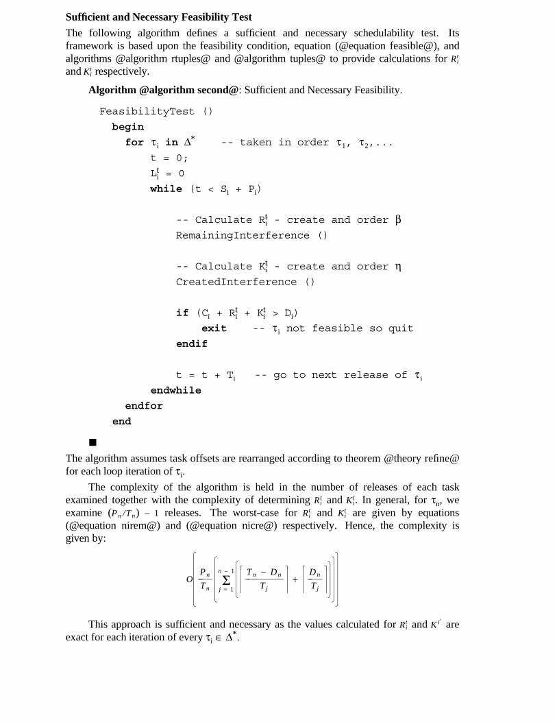
Sufficient and Necessary Feasibility Test

The following algorithm defines a sufficient and necessary schedulability test. Itsframework is based upon the feasibility condition, equation (@equation feasible@), andalgorithms @algorithm rtuples@ and @algorithm tuples@ to provide calculations for Ri

t

and Kit respectively.

Algorithm @algorithm second@: Sufficient and Necessary Feasibility.

FeasibilityTest ()

begin

for τ i in Δ* -- taken in order τ1, τ2,...

t = 0;

Lit = 0

while (t < Si + Pi)

-- Calculate Rit - create and order β

RemainingInterference ()

-- Calculate Kit - create and order η

CreatedInterference ()

if (Ci + Rit + Ki

t > Di)

exit -- τ i not feasible so quit

endif

t = t + Ti -- go to next release of τ i

endwhile

endfor

end

�The algorithm assumes task offsets are rearranged according to theorem @theory refine@for each loop iteration of τi.

The complexity of the algorithm is held in the number of releases of each taskexamined together with the complexity of determining Ri

t and Kit. In general, for τn, we

examine (Pn /Tn) − 1 releases. The worst-case for Rit and Ki

t are given by equations(@equation nirem@) and (@equation nicre@) respectively. Hence, the complexity isgiven by:

O

��

Tn

Pn��

��

j = 1Σ

n − 1��

�� Tj

Tn − Dn��

+�� Tj

Dn��

��

��

��

This approach is sufficient and necessary as the values calculated for Rit and Kit

areexact for each iteration of every τi ∈ Δ*.

Theorem @theory schedexact@:The schedulability test defined by equation (@equation feasible@) usingalgorithms @algorithm tuples@ and @algorithm rtuples@ for Ri

t and Kit

respectively is sufficient and necessary.

Proof:Consider τi ∈ Δ*. By theorem @theory interval@, if each release of τi in[S i , S i + Pi) meets its deadline, τi will always meet its deadline.

Consider the release of τi at t. In a static priority system, the only tasks that canprevent τi from meeting its deadline at t + Di are those higher priority tasks thatneed to execute in [t, t + Di). This is quantified as interference: Ri

t + Kit. Since

these values are exact, the test is sufficient and necessary.

�

5.2. Combining Priority Assignment and Feasibility Testing

The optimal priority assignment approach outlined in section 3 finds tasks feasible forpriority levels n, n − 1, ..., 1, in that order. The overall complexity of the combinedapproach is bounded by n times the complexity for determining the feasibility of τn, that is:

O

��

nTn

Pn��

��

j = 1Σ

n − 1��

�� Tj

Tn − Dn��

+�� Tj

Dn��

��

��

��

Consider the following task set.

Example @example exnon@:

τˆ(&sAˆ(&e : CA = 2 DA = 3 OA = 2 TA = 4

τˆ(&sBˆ(&e : CB = 3 DB = 4 OB = 0 TB = 8

τˆ(&sCˆ(&e : CC = 1 DC = 5 OC = 1 TC = 8

�Trivially the above is a non-critical instant task set. Firstly, we attempt to assign a task topriority level 3. Both τA and τB are infeasible at this level (for brevity we omit thecalculation). Consider τC at level 3 (arbitrarily we assign τA to 1 and τB to 2). Task offsetsare refined according to theorem @theory refine@: O1 = 1, O2 = 7 and O3 = 0. For τ3,Pi = 8 with S i = 8. Therefore, the feasibility interval is [8, 16) implying we must check thedeadline of the release of τ3 at 8:

Release of τ3 at 8:

Calculate R38. Since L3

0 = 0, tuple set β = {(2,2) , (2,6) , (3,7) } Stepping through time,we derive R3

8 = 2.

Calculate K38. Tuple set η = {(2,10) }. Stepping through time, we derive K3

8 = 2.

Giving R38 + K3

8 + C 3 = 5 = D3

Hence, if a feasible priority assignments exist for the task set, (at least) one willassign τC to priority level 3. The process of assignment and feasibility testingcontinues for levels 2 and 1, although is omitted for brevity. Tasks τB and τA areassigned levels 1 and 2 respectively and are feasible. An extended example is given

in the appendix.

6. CONCLUSIONS

This paper has considered and addressed several outstanding issues in static priorityscheduling theory for task sets containing tasks with arbitrary start times. Presented in thepaper have been efficient methods for

(i) determining if a set of tasks each with an arbitrary start time share a critical instant;

(ii) determining an optimal priority assignment;

(iii) determining feasibility.

Whilst no previous work is known to the authors regarding (i) and (ii), a comparison canbe drawn between (iii) and a feasibility test proposed by Leung, based upon theconstruction of a schedule for a pre-determined interval. We have reduced Leung’sinterval, so making the feasibility problem easier, as well as offering a more efficientfeasibility test for the reduced interval.

Whilst this paper presents a complete piece of work, further consideration of thefeasibility test may yield more efficiency. The theory provided in this paper, provides aspringboard for efficient solution of many problems that utilise task sets with arbitrary starttimes. Also, the theory in this paper is extensible. For example, it is the authors contentionthat the priority ceiling protocol theory [Sha90] can be incorporated trivially, thuspermitting tasks to block on resource access. Overall, the theory presented in this paperprovides a suitable vehicle for future research into the feasibility of even more generalisedand flexible static priority task sets containing tasks with arbitrary timing constraints.

REFERENCES

Aud90. N. C. Audsley, ‘‘Deadline Monotonic Scheduling’’, YCS 146, Department ofComputer Science, University of York (October 1990).

Aud91a. N. C. Audsley, A. Burns, M. F. Richardson and A. J. Wellings , ‘‘STRESS: ASimulator For Hard Real-Time System’’, RTRG/91/106, Real-Time ResearchGroup, Department of Computer Science, University of York (October 1991).

Aud91b. N. C. Audsley, A. Burns, M. F. Richardson and A. J. Wellings, ‘‘Hard Real-Time Scheduling: The Deadline Monotonic Approach’’, Proceedings 8th IEEEWorkshop on Real-Time Operating Systems and Software, Atlanta, GA, USA (15-17May 1991).

Jac75. T. H. Jackson, Number Theory, Routledge and Kegan Paul (1975).

Jos86. M. Joseph and P. Pandya, ‘‘Finding Response Times in a Real-Time System’’, TheComputer Journal (British Computer Society) 29(5), pp. 390-395, CambridgeUniversity Press (October 1986).

Knu73. D. E. Knuth, The Art of Computer Programming: Vol 1 Fundamental Algorithms,Addison-Wesley (2nd Edition 1973).

Leh90. J. P. Lehoczky, ‘‘Fixed Priority Scheduling of Periodic Task Sets With ArbitraryDeadlines’’, Proceedings 11th IEEE Real-Time Systems Symposium, Lake BuenaVista, FL, USA, pp. 201-209 (5-7 December 1990).

Leh89. J. Lehoczky, L. Sha and Y. Ding, ‘‘The Rate-Monotonic Scheduling Algorithm:Exact Characterization and Average Case Behaviour’’, Proceedings IEEE Real-Time Systems Symposium, Santa Monica, California, pp. 166-171, IEEE ComputerSociety Press (5-7 December 1989).

Leu89. J. Y. T. Leung, ‘‘A New Algorithm for Scheduling Periodic, Real-Time Tasks’’,Algorithmica 4, pp. 209-219 (1989).

Leu80. J. Y. T. Leung and M. L. Merrill, ‘‘A Note on Preemptive Scheduling of Periodic,Real-Time Tasks’’, Information Processing Letters 11(3) (November 1980).

Leu82. J. Y. T. Leung and J. Whitehead, ‘‘On the Complexity of Fixed-PriorityScheduling of Periodic, Real-Time Tasks’’, Performance Evaluation (Netherlands)2(4), pp. 237-250 (December 1982).

Liu73. C. L. Liu and J. W. Layland, ‘‘Scheduling Algorithms for Multiprogramming in aHard Real-Time Environment’’, Journal of the ACM 20(1), pp. 40-61 (1973).

Nas91. E. Nassor and G. Bres, ‘‘Hard Real-Time Sporadic Task Scheduling for FixedPriority Schedulers’’, Proceedings International Workshop on Responsive Systems,Golfe-Juan, France, pp. 44-47, INRIA (Institut National de Recherche enInformatique et en Automatique) (3-4 October 1991).

Ros85. K. H. Rosen, Elementary Number Theory and its Applications, Addison-Wesley(1985).

Sha90. L. Sha, R. Rajkumar and J. P. Lehoczky, ‘‘Priority Inheritance Protocols: AnApproach to Real-Time Synchronisation’’, IEEE Transactions on Computers 39(9),pp. 1175-1185 (September 1990).

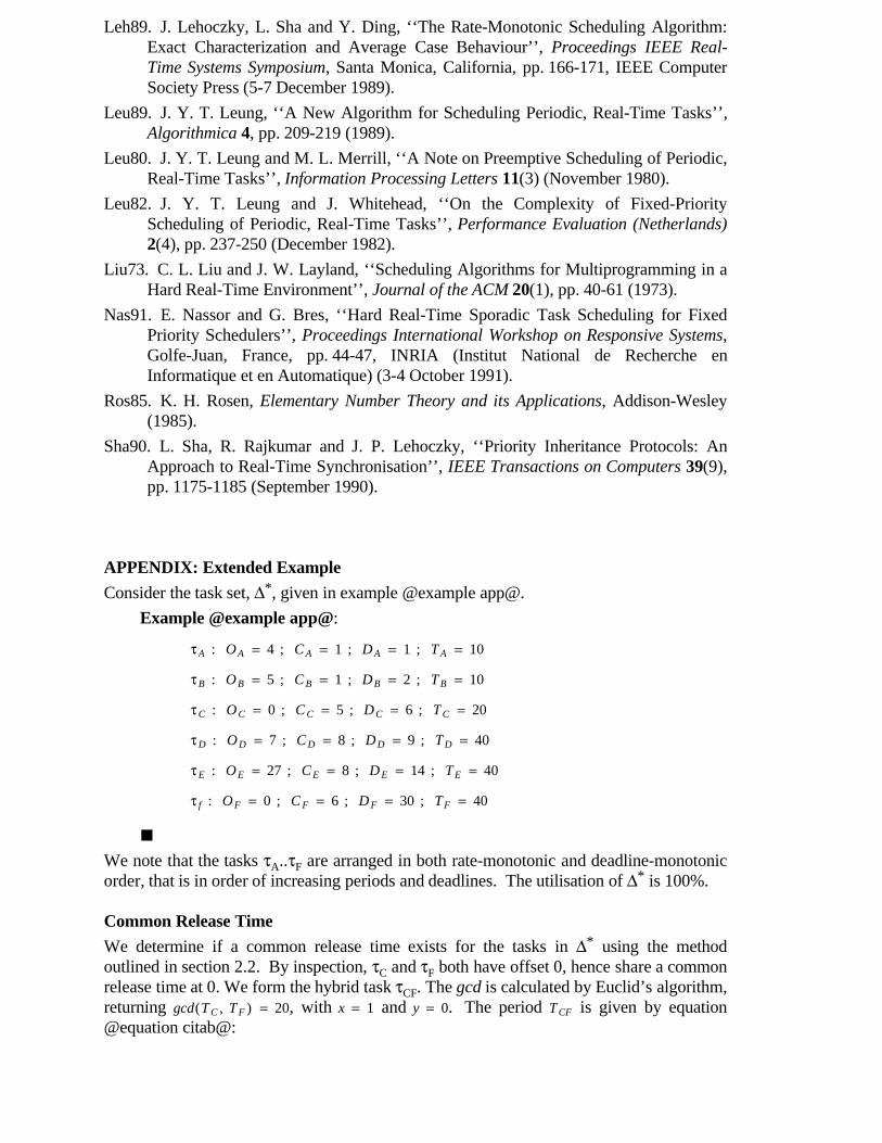
APPENDIX: Extended Example

Consider the task set, Δ*, given in example @example app@.

Example @example app@:

τA : OA = 4 ; CA = 1 ; DA = 1 ; TA = 10

τB : OB = 5 ; CB = 1 ; DB = 2 ; TB = 10

τC : OC = 0 ; CC = 5 ; DC = 6 ; TC = 20

τD : OD = 7 ; CD = 8 ; DD = 9 ; TD = 40

τE : OE = 27 ; CE = 8 ; DE = 14 ; TE = 40

τ f : OF = 0 ; CF = 6 ; DF = 30 ; TF = 40

�We note that the tasks τA..τF are arranged in both rate-monotonic and deadline-monotonicorder, that is in order of increasing periods and deadlines. The utilisation of Δ* is 100%.

Common Release Time

We determine if a common release time exists for the tasks in Δ* using the methodoutlined in section 2.2. By inspection, τC and τF both have offset 0, hence share a commonrelease time at 0. We form the hybrid task τCF. The gcd is calculated by Euclid’s algorithm,returning gcd(TC , TF ) = 20, with x = 1 and y = 0. The period TCF is given by equation@equation citab@:

TCF = TC gcd(TC , TF )

TF�� =20

20 × 40�� = 40

We now evaluate OCF. Evaluating k in equation (@equation Euclidk@), where h = 0,leaves k = 0. Evaluating t according to equation (@equation Euclidt@) leaves t = 0. Theoffset, OCF, given by equation @equation taskaboffset@ is OCF = 0, coninciding with thefirst common release of τC and τF.

Next, we consider if the hybrid task, τCF, shares a common release time with τA. Byequation @equation CriticalInstantCondition@ in section 2.1 we note that τCF and τA havea common release time if:

OA − OCF = h gcd(TA , TCF ) [h ∈ Z]

Since, by Euclid’s algorithm, gcd(TA , TCF ) = 40, h = 20/7 and so is not an integer. Thus τCFand τA, and therefore all the tasks in Δ* do not share a common release time.

Now, we move to consider the priority assignment and feasbility of the task set,according to the method established in sections 3 and 5: each priority level from 6 to 1 isassigned to a task in Δ*.

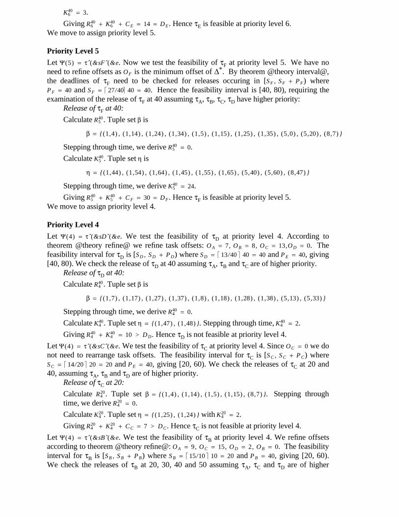
Priority Level 6

Let Ψ(6) = τˆ(&sFˆ(&e i.e. we wish to see if τF is feasible when assigned the lowestpriority. Now we test the feasibility of τF at priority level 6. We have no need to refineoffsets as OF is the minimum offset of Δ*. By theorem @theory interval@, the deadlinesof τF need to be checked for releases occuring in [SF , SF + PF) where PF = 40 andSF = � 27/40 � 40 = 40. Hence the feasibility interval is [40, 80), requiring the examinationof the release of τF at 40, assuming all other tasks have a higher priority:

Release of τF at 40:

Calculate R640. Tuple set β is

β = {(1,4) , (1,14) ,(1,24) , (1,34) , (1,5) , (1,15) , (1,25) , (1,35) ,

(5,0) , (5,20) , (8,7) , (8,27) }

Stepping through time, we derive R640 = 0 by algorithm @algorithm rtuples@.

Calculate K640. Tuple set η is:

η = {(1,44) , (1,54) , (1,64) , (1,45) , (1,55) , (1,65) , (5,40) , (5,60) , (8,47) , (8,67) }

Stepping through time, we derive K640 = 27 by algorithm @algorithm tuples@.

Giving R640 + K6

40 + CF = 33 > DF. Hence τF is not feasible at priority level 6.

Let Ψ(6) = τˆ(&sEˆ(&e. We test the feasibility of τE at priority level 6. According totheorem @theory refine@ we refine task offsets:OA = 7, OB = 8, OC = 13, OD = 20, OF = 13, OE = 0. The feasibility interval for τE is[SE , SE + PE) where SE = � 27/40 � 40 = 40 and PE = 40, giving [40, 80). We check therelease of τE at 40 assuming all other tasks have higher priority:

Release of τE at 40:


β = {(1,7) , (1,17) , (1,27) , (1,37) , (1,8) , (1,18) , (1,28) , (1,38) ,

(5,13) , (5,33) , (8,20) , (6,13) }

Stepping through time, we derive R640 = 3.

Calculate K640. Tuple set η = {(1,47) , (1,48) , (5,53) , (6,53) }. Stepping through time,

K640 = 3.

Giving R640 + K6

40 + CE = 14 = DE. Hence τE is feasible at priority level 6.We move to assign priority level 5.

Priority Level 5

Let Ψ(5) = τˆ(&sFˆ(&e. Now we test the feasibility of τF at priority level 5. We have noneed to refine offsets as OF is the minimum offset of Δ*. By theorem @theory interval@,the deadlines of τF need to be checked for releases occuring in [SF , SF + PF) wherePF = 40 and SF = � 27/40� 40 = 40. Hence the feasibility interval is [40, 80), requiring theexamination of the release of τF at 40 assuming τA, τB, τC, τD have higher priority:

Release of τF at 40:


β = {(1,4) , (1,14) , (1,24) , (1,34) , (1,5) , (1,15) , (1,25) , (1,35) , (5,0) , (5,20) , (8,7) }


Calculate K540. Tuple set η is

η = {(1,44) , (1,54) , (1,64) , (1,45) , (1,55) , (1,65) , (5,40) , (5,60) , (8,47) }

Stepping through time, we derive K540 = 24.

Giving R540 + K5

40 + CF = 30 = DF. Hence τF is feasible at priority level 5.We move to assign priority level 4.

Priority Level 4

Let Ψ(4) = τˆ(&sDˆ(&e. We test the feasibility of τD at priority level 4. According totheorem @theory refine@ we refine task offsets: OA = 7, OB = 8, OC = 13,OD = 0. Thefeasibility interval for τD is [SD , SD + PD) where SD = � 13/40 � 40 = 40 and PE = 40, giving[40, 80). We check the release of τD at 40 assuming τA, τB and τC are of higher priority.

Release of τD at 40:


β = {(1,7) , (1,17) , (1,27) , (1,37) , (1,8) , (1,18) , (1,28) , (1,38) , (5,13) , (5,33) }


Calculate K440. Tuple set η = {(1,47) , (1,48) }. Stepping through time, K4

40 = 2.

Giving R440 + K4

40 = 10 > DD. Hence τD is not feasible at priority level 4.

Let Ψ(4) = τˆ(&sCˆ(&e. We test the feasibility of τC at priority level 4. Since OC = 0 we donot need to rearrange task offsets. The feasibility interval for τC is [SC , SC + PC) whereSC = � 14/20 � 20 = 20 and PE = 40, giving [20, 60). We check the releases of τC at 20 and40, assuming τA, τB and τD are of higher priority.

Release of τC at 20:

Calculate R420. Tuple set β = {(1,4) , (1,14) , (1,5) , (1,15) , (8,7) }. Stepping through

time, we derive R420 = 0.

Calculate K420. Tuple set η = {(1,25) , (1,24) } with K4

20 = 2.

Giving R420 + K4

20 + CC = 7 > DC. Hence τC is not feasible at priority level 4.

Let Ψ(4) = τˆ(&sBˆ(&e. We test the feasibility of τB at priority level 4. We refine offsetsaccording to theorem @theory refine@: OA = 9, OC = 15, OD = 2, OB = 0. The feasibilityinterval for τB is [SB , SB + PB) where SB = � 15/10 � 10 = 20 and PB = 40, giving [20, 60).We check the releases of τB at 20, 30, 40 and 50 assuming τA, τC and τD are of higher

priority.Release of τB at 20:

Calculate R420. Tuple set β = {(1,9) , (1,19) , (5,15) , (8,2) }. Stepping through time, we

derive R420 = 1.

Calculate K420. Since tuple set η = {}, K4

20 = 0.

Giving R420 + K4

20 + CB = 2 = DB. Hence τB is feasible at priority level 4 for therelease at 20.Release of τB at 30:

Calculate R430. We note that L4

21 = 0, that is the remaining workload of τA, τC and τD atthe deadline of the release of τB at 20 was 0. Tuple set β = {(1,29) }. Steppingthrough time, we derive R4

30 = 0.


30 = 0.

Giving R430 + K4

30 + CB = 1 < DB. Hence τB is feasible at priority level 4 for therelease at 30.Release of τB at 40:


31 = 0, that is the remaining workload of τA, τC and τD atthe deadline of the release of τB at 30 was 0. Tuple set β = {(1,39) , (5,35) }. Steppingthrough time, R4

40 = 1.


40 = 0.

Giving R440 + K4

40 + CB = 2 = DB. Hence τB is feasible at priority level 4 for therelease at 40.Release of τB at 50:


41 = 0, that is the remaining workload of τA, τC and τD atthe deadline of the release of τB at 40 was 0. Tuple set β = {(8,42) , (1,49) }. Steppingthrough time, R4

40 = 1.


50 = 0.

Giving R450 + K4

50 + CB = 2 = DB. Hence τB is feasible at priority level 4 for therelease at 50. Therefore, τB is feasible for releases at 20, 30, 40 and 50 and so isfeasible at priority level 4.

We move to assign priority level 3.

Priority Level 3

Let Ψ(3) = τˆ(&sDˆ(&e. We test the feasibility of τD at priority level 3. We refine offsetsaccording to theorem @theory refine@: OA = 7, OC = 13, OD = 0. The feasibility intervalfor τD is [SD , SD + PD) where SD = � 13/40 � 40 = 40 and PB = 40, giving [40, 80). Wecheck the release of τD at 40, assuming τA and τC are of higher priority.

Release of τD at 40:

Calculate R440. Tuple set β = {(1,7) , (1,17) , (1,27) , (1,37) , (6,13) , (6,33) }. Stepping

through time, we derive R440 = 0.

Calculate K440. Tuple set η = {(1,47) }. Stepping through time, K4

40 = 1.

Giving R440 + K4

40 + CD = 9 = DD. Hence τD is feasible at priority level 3.We move to priority level 2.

Priority Level 2

Let Ψ(2) = τˆ(&sCˆ(&e. We test the feasibility of τC at priority level 2. There is no need torefine deadlines according to theorem @theory refine@ as OC = 0. The feasibility intervalfor τC is [SC , SC + PC) where SC = � 14/20 � 20 = 20 and PC = 20, giving [20, 40). We checkthe release of τC at 20, assuming τA is of higher priority.

Release of τC at 20:

Calculate R420. Tuple set β = {(1,4) , (1,14) }. Stepping through time, we derive

R420 = 0.

Calculate K420. Tuple set η = {(1,24) }. Stepping through time, we derive K4

20 = 1.

Giving R440 + K4

40 + CC = 6 = DC. Hence τD is feasible at priority level 2.We move to priority level 1.

Priority Level 1

One unassigned task remains, hence let Ψ(1) = τˆ(&sAˆ(&e. Refining offsets, OA = 0. Thefeasiblity interval is [SA , SA + PA) where SA = � 0/10 � 10 = 0 and PA = TA = 10, giving [0,10). We check the release os τA at 0 only. Trivially, since no higher priority tasks exist,R1

0 = K10 = 0, giving CA = 1 = DA. Thus τA is feassible at priority level 1.

Summary

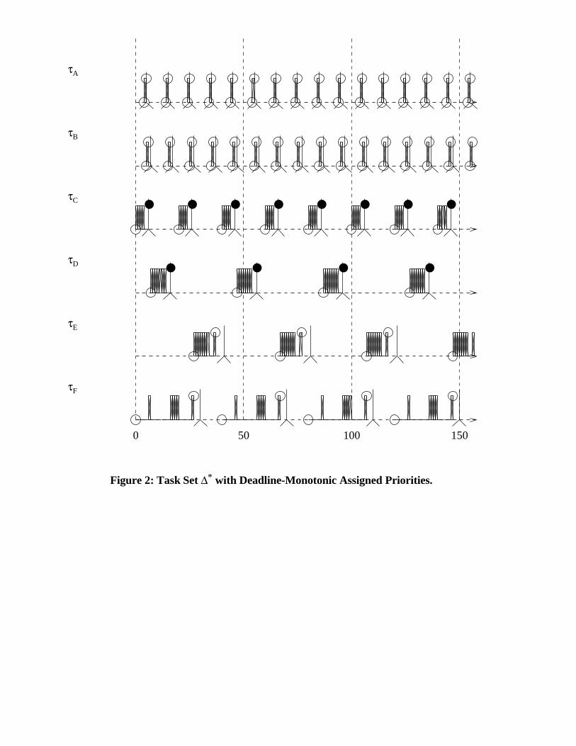
The task set Δ* is feasible with Ψ(1) = τˆ(&sAˆ(&e, Ψ(2) = τˆ(&sCˆ(&e,Ψ(3) = τˆ(&sDˆ(&e, Ψ(4) = τˆ(&sBˆ(&e, Ψ(5) = τˆ(&sFˆ(&e and Ψ(6) = τˆ(&sEˆ(&e.Figure 1 shows a simulation of task set Δ* illustrating that no deadlines are missed whenthe above priority assignment is used. In contrast, Figure 2 shows the result of usingdeadline-montonic priority ordering: tasks miss deadlines. The figures are produced usingthe STRESS real-time simulator [Aud91a]. In both figures, time increases horizontally tothe right, with individual dashed timelines shown for each task. Tasks have solidhorizontal times whilst preempted. Task releases are given by a circle on the timeline;execution by a hatched box; task completion by a raised circle. Deadlines are indicated bya vertical solid line with an arrow head on the timeline. Missed deadlines are shown by araised solid bullet.

0 50 100 150

τA

τC

τD

τB

τF

τE

Figure 1: Task Set Δ* with Optimally Assigned Priorities.

�

�

� �

�

� �

�

� �

�

�

0 50 100 150

τA

τB

τC

τD

τE

τF

Figure 2: Task Set Δ* with Deadline-Monotonic Assigned Priorities.

optimal priority assignment and feasibility of static priority tasks with arbitrary start times

Documents