optimal project portfolio execution -...

Optimal Project Portfolio Execution

Using analytical and simulation models with realistic project layouts and resource behaviour

O L A J O H A N N E S S O N C H R I S T O F E R J O H A N S S O N H I I T T I

Master of Science Thesis Stockholm, Sweden 2014


Using analytical and simulation models with realistic project layouts and resource behaviour

O L A J O H A N N E S S O N

C H R I S T O F E R J O H A N S S O N H I I T T I

Master’s Thesis in Systems Engineering (30 ECTS credits) Master Programme in Aerospace Engineering (120 credits) Royal Institute of Technology year 2014 Supervisor at KTH was Per Enqvist Examiner was Per Engvist TRITA-MAT-E 2014:04 ISRN-KTH/MAT/E--14/04--SE Royal Institute of Technology School of Engineering Sciences KTH SCI SE-100 44 Stockholm, Sweden URL: www.kth.se/sci


Using analytical and simulation models with realistic project layouts and resourcebehaviour

OLA JOHANNESSON 890502-0635CHRISTOFER JOHANSSON HIITTI 891018-8534

Master’s Thesis at SCISupervisor: Per EnqvistExaminer: Per Enqvist

TRITA xxx yyyy-nn

iii

Abstract

This project aims to increase the knowledge in the area of resource alloca-tion in R&D portfolios, a topic interesting to both the industry and academicresearch. The thesis investigates how to optimally allocate resources to projectsin a R&D portfolio, with focus on how many projects that are optimal to runin parallel. A complex mixed-integer nonlinear programming model with arealistic stage-gate project layout and advanced resource behaviour, includ-ing project resource learning and other efficiency losses, is developed and alsoproven unsolvable in realistic time. A simplified model handling learning isproposed and solved using a mixed integer solver for a small portfolio. A simu-lation framework implementing all complexities is developed, and used to findportfolio parameters affecting the optimal number of projects to run in parallel,using a Monte Carlo method.

From the simplified mathematical model optimal allocations from smallportfolios are presented, and from the simulation several results from largeportfolios using different resource allocation strategies are presented. Fromthese results it is argued that there exists an optimal number of projects to runin a portfolio, and that a portfolio run with either larger or smaller numberof running projects produces a lower gain. This number is however found tobe highly dependent on the size and specification of the portfolio, and howresources are allocated to projects.

iv

Sammanfattning

Detta masterarbete har som mål att utöka kunskapen kring resursallokeringinom portföljer med utvecklingsprojekt, ett område som genererat intresse bådeinom industrin och inom tidigare akademiska arbeten. Rapporten undersökerhur resurser optimalt ska allokeras till projekt inom utvecklingsportföljer, medhuvudsakligt fokus på hur många projekt som är optimalt att köra på sammagång. Ett ickelinjärt mixed-integer optimeringsproblem, som bygger på en re-alistisk stage-gate projektmodell samt avancerade approximationer av resusersbeteende, ställs upp; modellen inkluderar bland annat lärotider vid allokeringtill nya projekt och andra effektivitetsförluster. Denna modell bevisas olösbarmed realistisk beräkningskraft. En förenklad modell som tar hänsyn till läran-deeffekterna tas fram och löses för små portföljer. Ett simuleringsprogram tasockså fram vilket inkluderar all komplexitet från den fullständiga modellen, ochdetta används för att med en Monte Carlo-metod undersöka vilka portföljpa-rametrar som påverkar hur många projekt som optimalt ska köras parallellt.

Från den förenklade matematiska modellen tas optimala resursfördelningarfram för små portföljer, och från simuleringarna presenteras data från realistisktstora portföljer vilka har simulerats med olika resursallokeringsstrategier. Dessaresultat visar på att det finns ett optimalt antal projekt att köra parallellt ien portfölj, och att om en portfölj drivs med antingen färre eller fler projektparallellt ger det en lägre vinst. Exakt vad detta optimala antal projekt är berordock mycket på storleken och detaljer i portföljen, och hur resurser allokerastill projekt.

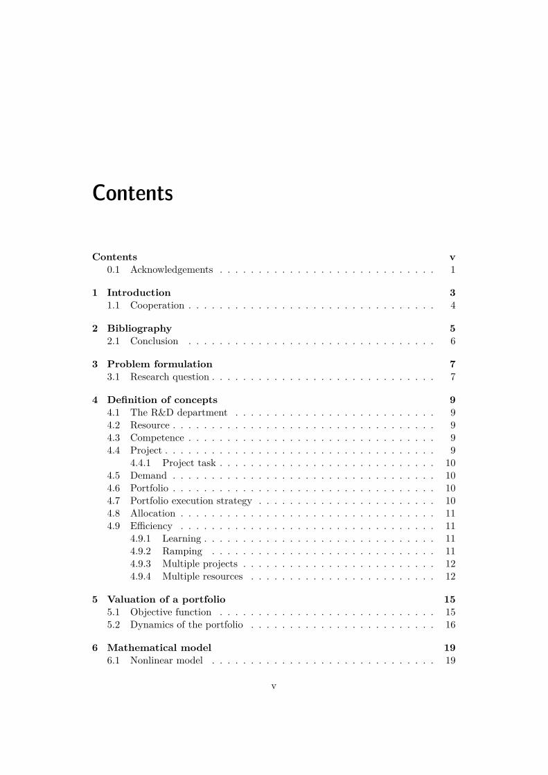
Contents

Contents v0.1 Acknowledgements . . . . . . . . . . . . . . . . . . . . . . . . . . . . 1

1 Introduction 31.1 Cooperation . . . . . . . . . . . . . . . . . . . . . . . . . . . . . . . . 4

2 Bibliography 52.1 Conclusion . . . . . . . . . . . . . . . . . . . . . . . . . . . . . . . . 6

3 Problem formulation 73.1 Research question . . . . . . . . . . . . . . . . . . . . . . . . . . . . . 7

4 Definition of concepts 94.1 The R&D department . . . . . . . . . . . . . . . . . . . . . . . . . . 94.2 Resource . . . . . . . . . . . . . . . . . . . . . . . . . . . . . . . . . . 94.3 Competence . . . . . . . . . . . . . . . . . . . . . . . . . . . . . . . . 94.4 Project . . . . . . . . . . . . . . . . . . . . . . . . . . . . . . . . . . . 9

4.4.1 Project task . . . . . . . . . . . . . . . . . . . . . . . . . . . . 104.5 Demand . . . . . . . . . . . . . . . . . . . . . . . . . . . . . . . . . . 104.6 Portfolio . . . . . . . . . . . . . . . . . . . . . . . . . . . . . . . . . . 104.7 Portfolio execution strategy . . . . . . . . . . . . . . . . . . . . . . . 104.8 Allocation . . . . . . . . . . . . . . . . . . . . . . . . . . . . . . . . . 114.9 Efficiency . . . . . . . . . . . . . . . . . . . . . . . . . . . . . . . . . 11

4.9.1 Learning . . . . . . . . . . . . . . . . . . . . . . . . . . . . . . 114.9.2 Ramping . . . . . . . . . . . . . . . . . . . . . . . . . . . . . 114.9.3 Multiple projects . . . . . . . . . . . . . . . . . . . . . . . . . 124.9.4 Multiple resources . . . . . . . . . . . . . . . . . . . . . . . . 12

5 Valuation of a portfolio 155.1 Objective function . . . . . . . . . . . . . . . . . . . . . . . . . . . . 155.2 Dynamics of the portfolio . . . . . . . . . . . . . . . . . . . . . . . . 16

6 Mathematical model 196.1 Nonlinear model . . . . . . . . . . . . . . . . . . . . . . . . . . . . . 19

v

vi CONTENTS

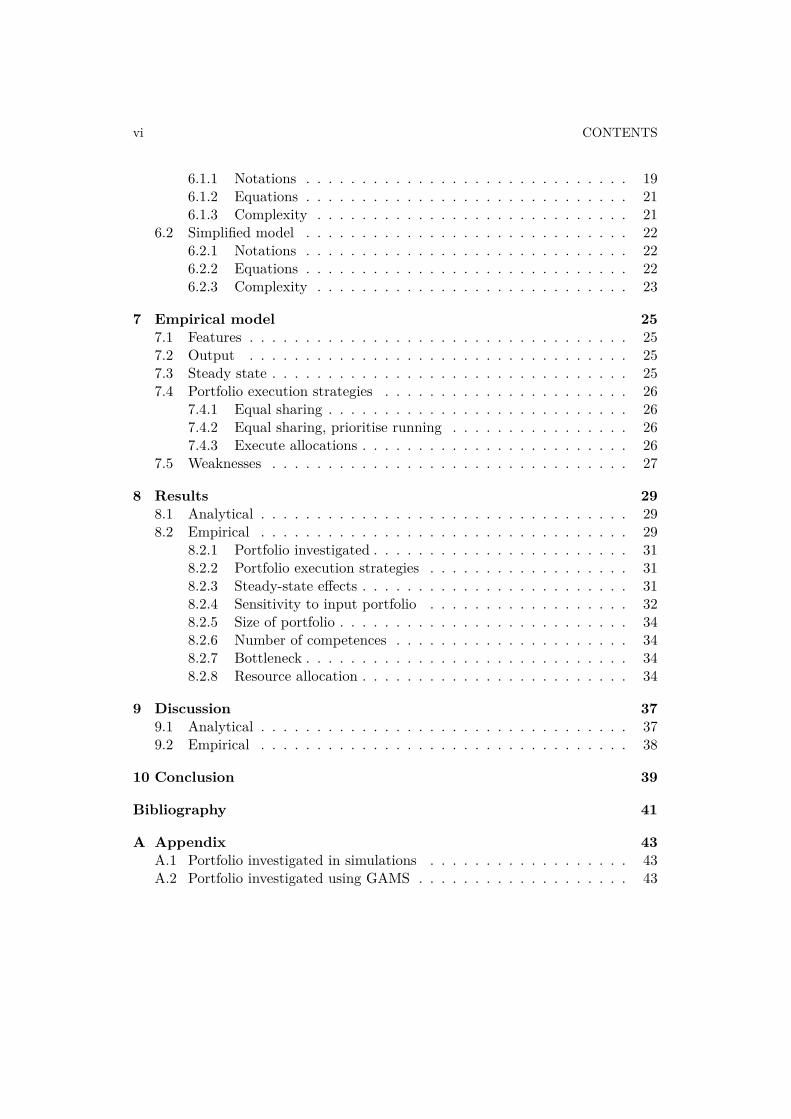
6.1.1 Notations . . . . . . . . . . . . . . . . . . . . . . . . . . . . . 196.1.2 Equations . . . . . . . . . . . . . . . . . . . . . . . . . . . . . 216.1.3 Complexity . . . . . . . . . . . . . . . . . . . . . . . . . . . . 21

6.2 Simplified model . . . . . . . . . . . . . . . . . . . . . . . . . . . . . 226.2.1 Notations . . . . . . . . . . . . . . . . . . . . . . . . . . . . . 226.2.2 Equations . . . . . . . . . . . . . . . . . . . . . . . . . . . . . 226.2.3 Complexity . . . . . . . . . . . . . . . . . . . . . . . . . . . . 23

7 Empirical model 257.1 Features . . . . . . . . . . . . . . . . . . . . . . . . . . . . . . . . . . 257.2 Output . . . . . . . . . . . . . . . . . . . . . . . . . . . . . . . . . . 257.3 Steady state . . . . . . . . . . . . . . . . . . . . . . . . . . . . . . . . 257.4 Portfolio execution strategies . . . . . . . . . . . . . . . . . . . . . . 26

7.4.1 Equal sharing . . . . . . . . . . . . . . . . . . . . . . . . . . . 267.4.2 Equal sharing, prioritise running . . . . . . . . . . . . . . . . 267.4.3 Execute allocations . . . . . . . . . . . . . . . . . . . . . . . . 26

7.5 Weaknesses . . . . . . . . . . . . . . . . . . . . . . . . . . . . . . . . 27

8 Results 298.1 Analytical . . . . . . . . . . . . . . . . . . . . . . . . . . . . . . . . . 298.2 Empirical . . . . . . . . . . . . . . . . . . . . . . . . . . . . . . . . . 29

8.2.1 Portfolio investigated . . . . . . . . . . . . . . . . . . . . . . . 318.2.2 Portfolio execution strategies . . . . . . . . . . . . . . . . . . 318.2.3 Steady-state effects . . . . . . . . . . . . . . . . . . . . . . . . 318.2.4 Sensitivity to input portfolio . . . . . . . . . . . . . . . . . . 328.2.5 Size of portfolio . . . . . . . . . . . . . . . . . . . . . . . . . . 348.2.6 Number of competences . . . . . . . . . . . . . . . . . . . . . 348.2.7 Bottleneck . . . . . . . . . . . . . . . . . . . . . . . . . . . . . 348.2.8 Resource allocation . . . . . . . . . . . . . . . . . . . . . . . . 34

9 Discussion 379.1 Analytical . . . . . . . . . . . . . . . . . . . . . . . . . . . . . . . . . 379.2 Empirical . . . . . . . . . . . . . . . . . . . . . . . . . . . . . . . . . 38

10 Conclusion 39

Bibliography 41

A Appendix 43A.1 Portfolio investigated in simulations . . . . . . . . . . . . . . . . . . 43A.2 Portfolio investigated using GAMS . . . . . . . . . . . . . . . . . . . 43

0.1. ACKNOWLEDGEMENTS 1

0.1 AcknowledgementsWe would like to express our very great appreciation to Mattias Nordin in AtlasCopco, Lars Cederblad in Level 21 and Per Enquist in KTH for making this thesishappen and guiding us through the project in their roles as our supervisors. Wewould also like to extend our thanks to Bengt Hallberg in Level 21 and Jan Kalanderin Atlas Copco for their constructive inputs on many parts of this project.

Introduction

In a Research and Development (R&D) department, as in every project-driven en-vironment, the question of how to select and run a project portfolio arises. How thisquestion is answered highly affects the output from the portfolio. The problem canbe divided into two parts, one concerned with optimal portfolio selection and onetreating project scheduling and resource allocation in such an optimal portfolio. Inoptimal portfolio theory simplified economic models are developed for the projects,often describing expected profit and associated risk, and then the combination ofthese giving optimal profit under certain boundary conditions are calculated. Theallocation problem is in its basic form a relatively simple problem with well-knownsolutions [7]. Models that combine both these steps have been proposed, but havehad the downside of being highly simplified in order to be solvable [4].

In practice the different project portfolio selection tools and theories are widelyused and implemented as company policies. However the use of advanced modelsfor portfolio execution and staff allocation is limited, instead strategies such asmaximizing resource utilization instead of R&D output are widely used, accordingto experts in Atlas Copco and Level 21 Management. A major problem with themodels come from the simplifications done when describing projects, the portfolioand the environment that it is executed in. These simplifications most notablyinclude only looking at one competence, or a project description with fixed run timeand fixed work demand over time. Models with these limitations provide limiteduse in real-life multi-competence environments with flexible deadlines. They alsolack the possibility to study one of the main portfolio management variables, theeffect of the number of projects running simultaneously.

In order to further understand the execution of portfolios in a complex envi-ronment a model capable of describing realistic projects, with demands for multiplecompetences, will be presented in this paper. The project model makes use of a taskbased internal model to give support for advanced project descriptions; it is focusedon project following a stage-gate model, a model widely used in R&D projects [8].The model presented optimises for maximum future profit from the project portfo-lio. From this model both an optimisation problem and a simulation framework areformed, and a combination of these are used to examine the behaviour of optimalsolutions. The existence of a global optimal solution is examined for small problems,and proposals and evaluation of practically usable allocation strategies are made.

The model is based on information from the large multinational manufacturing

3

4 CHAPTER 1. INTRODUCTION

company Atlas Copco and knowledge from Level 21 Management, and the model ismost suited for similar organizations with a large project-base and several projectsrunning at any given time.

1.1 CooperationThe project and research on which this report builds was made in a team consistingof the two authors of this report and Elhabib Moustaid. A report titled OptimalProject Portfolio Execution - Computer Implementation of Models and SimulationFramework [9] is also available covering the same models and implementations, butwith further focus on the computer implementations and solutions.

Bibliography

Solving the portfolio execution and resource allocation problem is highly desiredby companies and is thus subject to research by the scientific community. Theresearch in this field is extensive and broad since there are many different waysto model the problem, and several special cases that can be considered. Earlierworks and publications in the area are mostly focused on choosing and schedulingprojects for a portfolio, however the resource allocation problem has been studiedas well. Studies have been done handling the individual resources in respect toknowledge and learning associated with being allocated to certain projects, andothers considering resources as a source of costs and thus treating budget allocationsover time.

Ghasemzadeh et. al [4] propose a way to select possible projects to a projectportfolio to be executed. They also propose the scheduling of those projects withinthe portfolio with a varying consumption of resources. They solve this using a Zero-one integer linear programming model, however they are scheduling projects witha fixed run time.

Solak et. al [1] looks at the problem differently and argues that the problemneeds to be modeled as a multistage stochastic integer problem. They introduceuncertainty about the running projects which needs to be progressively learnt duringproject execution, the unknown variable is the work required. They also introduceproject dependencies, that one project may not be started before a knowledge in itstechnology is filled by another project. They identify the full multistage problemto be NP-hard and reduce it by going from multistage to a two-stage problemwhich they later solve by a sample average approximation method of Lagrangianrelaxation and a new lower bounding heuristic. However they limit the problem toone competence.

Kira et. al [6] investigates a neighbouring project selection and allocation prob-lem to R&D projects, namely IS projects (Information system, software and hard-ware decisions) under risk. They use linear programming to solve the problem andconducts extensive analysis about the effect of uncertainty due to unknown vari-ables, project work demand etc, using Monte Carlo simulation. They also develop aSpecific Decision Support System to aid management decision making guided fromtheir results.

Matt Bassett [2] investigates how to optimally assign project tasks to people inrespect to utilization of their expertise and hiring outside resources. He uses heuris-

5

6 CHAPTER 2. BIBLIOGRAPHY

tic to quickly give a feasible solution to the problem of globally assigning peopleto the available tasks and also a mathematical program which is more rigorous.However he is assuming a fixed consumption of resources.

Certa et. al [5] focuses on fixed-time-frame completion of multiple projects andtreats learning effects and social interaction effects. They use multi-skilled resourcesin their model. This leads to the problem being multi-objective since knowledge anddevelopment of the resources is as desired as pure monetary output from a portfolioexecution.

The stage gate model for project execution, first described by Cooper in 1990[3], describes how a project can be separated into a number of sequentially executedparts (stages) with control checkpoints between them (gates). He argues that animportant factor in the model is parallel execution of activities involving differentfunctions in the firm. Through case-studies in multiple companies Högman et. al.finds that the stage gate model is widely used mainly in product development, butalso is implemented in technology development with some slight modifications [8].

2.1 ConclusionIn previous work the focus has been mainly on project selection and scheduling[1][6][5], and in some cases simple allocation models. The resource allocation prob-lem has however been studied previously, both in its basic form [1][6] and incorpo-rating extensions such as knowledge accumulation [5] and hiring external resources[2]. All of these does however work with a simple model for projects, and by inves-tigating the behaviour of a portfolio with multiple competences and an advancedproject model [3] this paper seeks to contribute new knowledge to the field.

Problem formulation

As presented in Section 2.1 the main focus on previous research in portfolio execu-tion has been that of allocating resources to projects with fixed run time. This ishowever a simplification that limits the optimal solution. A dynamic project execu-tion time allows for further freedom in the model and thus constitutes an approachto the optimal solution to the portfolio execution and allocation problem. With thismodel that gives a higher degree of freedom in portfolio execution the possibilityarises to study phenomena previously hidden in simplifications.

In both Atlas Copco and Level 21 Management there has been expressed concernthat there might be a tendency in R&D departments to start too many projects,and for this reason the report aims to extend the knowledge of portfolio executionand resource allocation in ways that helps answer this question.

3.1 Research questionBased in this a main research question and two important sub questions are iden-tified:

• Given a R&D portfolio, does it exist an optimal number of running projects,in the sense that gives the highest profit?

• If so, what is this number for a given R&D portfolio?

• How does the portfolio composition affect this number?

7

Definition of concepts

In the description of a R&D department and the running of projects a number ofconcepts are necessary, in this chapter all major concepts are defined for use in thispaper.

4.1 The R&D departmentA Research and Development (R&D) department is consistently in this paper mod-elled as one with a predefined constant work force. The department is assumed tobe a multi competence environment, where resources are divided into groups basedon their main competence, and a project might need resources from several differentcompetence groups to be completed.

4.2 ResourceA resource is one person working in the R&D department; a resource has a fixedamount of available work hours per week, to be allocated to projects. The resourceis defined to work in only one area, and thus belongs to one single competencegroup. Dividing resources by competence is a simplification not done in all previousresearch [5], however it is valid for the R&D department in Atlas Copco and manycompanies with them.

4.3 CompetenceA competence is a skill type, or a knowledge area, and a resource of a specificcompetence can only produce work on a project task with matching competence.

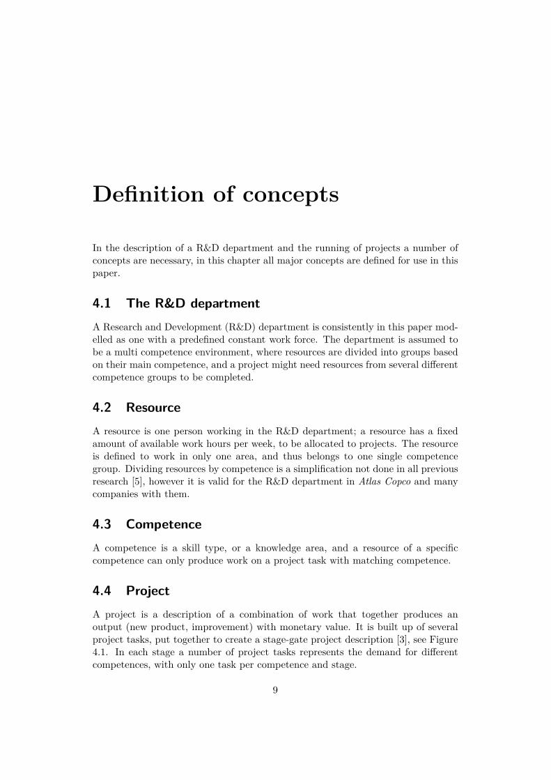
4.4 ProjectA project is a description of a combination of work that together produces anoutput (new product, improvement) with monetary value. It is built up of severalproject tasks, put together to create a stage-gate project description [3], see Figure4.1. In each stage a number of project tasks represents the demand for differentcompetences, with only one task per competence and stage.

9

10 CHAPTER 4. DEFINITION OF CONCEPTS

Figure 4.1. State gate project

4.4.1 Project task

A project task is a part of a project, with demand of one single competence. Itis defined to be finished when the work done on the tasks exceeds its demand. Atask may have dependencies on other project tasks in such a way that it cannot bestarted before its dependency tasks are done.

4.5 Demand

Demand is the amount of work required for a project task, and is measured in workhours with perfect efficiency. Because the efficiency is usually lower, the amount ofallocated man work hours required to finish a task usually exceeds its demand.

4.6 Portfolio

A portfolio is a grouping of multiple projects that are desired to be run in theR&D department. They are assumed to be preselected using portfolio selectiontechniques and to be ordered in the desired run order by some other part of thecompany, for example marketing or higher management. However it is assumedthat no project dependency exists so the projects execution order is free. In theportfolios used all projects share the same basic layout of tasks and is describedby a stage-gate model, see A.1. The total demand for all competences are scaleddifferently to create projects of different sizes.

4.7 Portfolio execution strategy

Portfolio execution strategies are heuristic algorithms for allocating resources toprojects.

4.8. ALLOCATION 11

0 1 2 3 0

0.2

0.4

0.6

0.8

1

Learning

Weeks into new project

Eff

ice

ncy

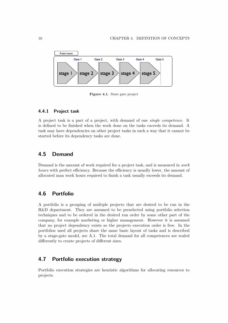
Figure 4.2. Effect of learning

4.8 Allocation

An allocation is a link between a resource and a project, it describes how many hoursa resource will devote to a specific project task in a week. Because of efficiency thisis however not necessarily the amount of work the resource do on the task.

4.9 Efficiency

Even if a resource is working fully in a project task, the actual work produced willnot necessarily be the same as what is allocated. The amount of work produced willvary with a number of efficiency functions, described below. These functions havebeen developed in cooperation with the R&D portfolio management team in AtlasCopco and experts in Level 21 Management. The total efficiency is the productof all efficiency functions evaluated for a resource-task combination. As several ofthese functions are non-convex the total efficiency function is also non-convex.

4.9.1 Learning

A resource will not work fully if it does not know the project, it needs to learn it,thus efficiency loss, see Figure 4.2. If a resource have not been working on a projectfor a while it will start to lose its knowledge and thus needing to learn again, seeFigure 4.3.

4.9.2 Ramping

When new resource are allocated to a project old resources will need to take timefrom their productive work time to teach the new resources, thus efficiency loss on

12 CHAPTER 4. DEFINITION OF CONCEPTS

Figure 4.3. Effect of loosing learning

Figure 4.4. Effect of ramping

all old resources. The efficiency loss is proportional to the ratio of new and oldresources, see Figure 4.4.

4.9.3 Multiple projects

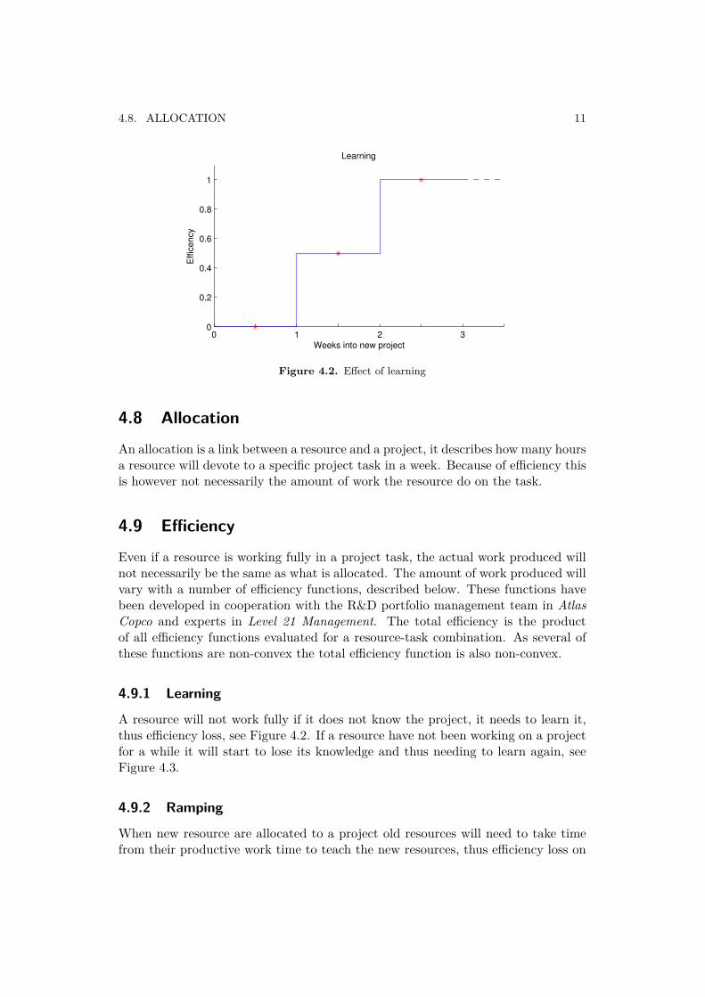
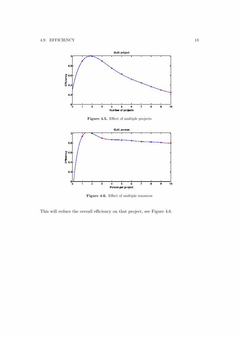
When a resource is working on multiple projects its overall efficiency will be affected.This is due to the fact that the resource needs switch projects during the workingweek which introduces some overhead work. It can also be a positive change inefficiency since if one project is stuck the resource can work on another, see Figure4.5.

4.9.4 Multiple resources

If there are many resources working on a project the project needs more overhead,such as team leaders and groups, and also more time will be spent in group meetings.

4.9. EFFICIENCY 13

Figure 4.5. Effect of multiple projects

Figure 4.6. Effect of multiple resources

This will reduce the overall efficiency on that project, see Figure 4.6.

Valuation of a portfolio

An important aspect of optimising a project portfolio is deciding the criteria foroptimality. In this paper the chosen measurement is purely economical, in otherwords the optimal portfolio is the one that gives the company the highest futuremonetary value.

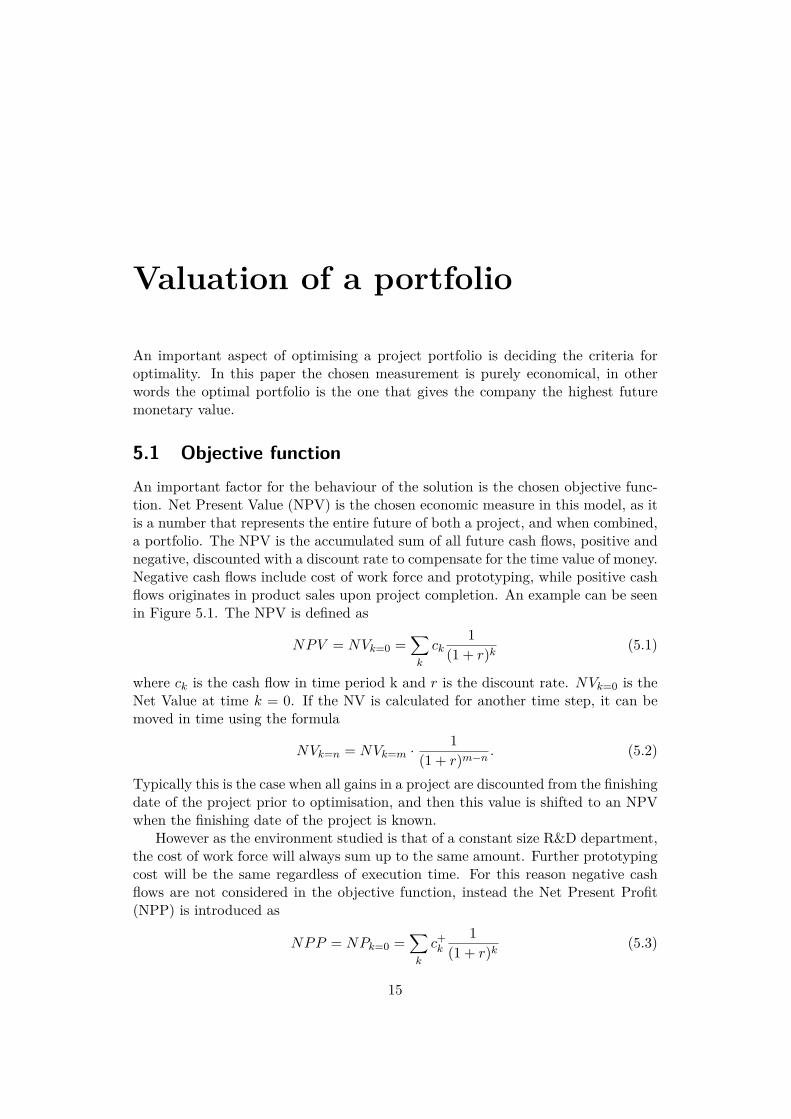
5.1 Objective functionAn important factor for the behaviour of the solution is the chosen objective func-tion. Net Present Value (NPV) is the chosen economic measure in this model, as itis a number that represents the entire future of both a project, and when combined,a portfolio. The NPV is the accumulated sum of all future cash flows, positive andnegative, discounted with a discount rate to compensate for the time value of money.Negative cash flows include cost of work force and prototyping, while positive cashflows originates in product sales upon project completion. An example can be seenin Figure 5.1. The NPV is defined as

NPV = NVk=0 =∑

k

ck1

(1 + r)k(5.1)

where ck is the cash flow in time period k and r is the discount rate. NVk=0 is theNet Value at time k = 0. If the NV is calculated for another time step, it can bemoved in time using the formula

NVk=n = NVk=m ·1

(1 + r)m−n. (5.2)

Typically this is the case when all gains in a project are discounted from the finishingdate of the project prior to optimisation, and then this value is shifted to an NPVwhen the finishing date of the project is known.

However as the environment studied is that of a constant size R&D department,the cost of work force will always sum up to the same amount. Further prototypingcost will be the same regardless of execution time. For this reason negative cashflows are not considered in the objective function, instead the Net Present Profit(NPP) is introduced as

NPP = NPk=0 =∑

k

c+k

1(1 + r)k

(5.3)

15

16 CHAPTER 5. VALUATION OF A PORTFOLIO

Figure 5.1. Cash flows over time for a project

where c+k is the positive cash flow in period k. The cash flows can be either those

for one project, or the accumulated cash flow for a full portfolio. The NP can beshifted as described in function (5.2).

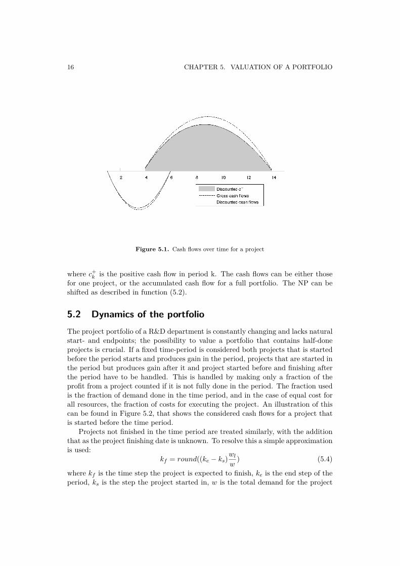
5.2 Dynamics of the portfolioThe project portfolio of a R&D department is constantly changing and lacks naturalstart- and endpoints; the possibility to value a portfolio that contains half-doneprojects is crucial. If a fixed time-period is considered both projects that is startedbefore the period starts and produces gain in the period, projects that are started inthe period but produces gain after it and project started before and finishing afterthe period have to be handled. This is handled by making only a fraction of theprofit from a project counted if it is not fully done in the period. The fraction usedis the fraction of demand done in the time period, and in the case of equal cost forall resources, the fraction of costs for executing the project. An illustration of thiscan be found in Figure 5.2, that shows the considered cash flows for a project thatis started before the time period.

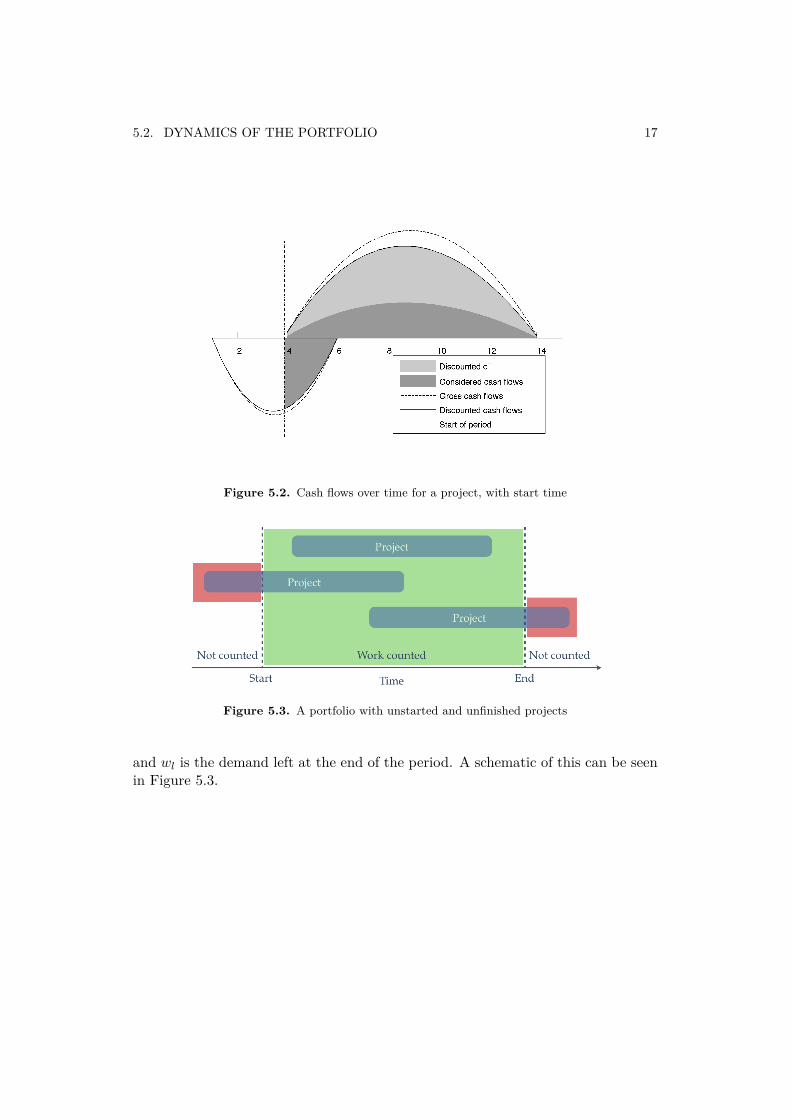
Projects not finished in the time period are treated similarly, with the additionthat as the project finishing date is unknown. To resolve this a simple approximationis used:

kf = round((ke − ks)wl

w) (5.4)

where kf is the time step the project is expected to finish, ke is the end step of theperiod, ks is the step the project started in, w is the total demand for the project

5.2. DYNAMICS OF THE PORTFOLIO 17

Figure 5.2. Cash flows over time for a project, with start time

Figure 5.3. A portfolio with unstarted and unfinished projects

and wl is the demand left at the end of the period. A schematic of this can be seenin Figure 5.3.

Mathematical model

In order to gain understanding of the problem mathematical problems are formu-lated for both the full problem with all nonlinearities and arbitrary task dependen-cies. A simplified model that is practically solvable is also presented.

6.1 Nonlinear modelThe model aims to capture the full complexity of the R&D portfolio allocationproblem, and thus include all concept previously discussed. That includes arbitrarytask dependencies and all nonlinearities. First the notation will be presented, thenthe equations are presented and explained.

6.1.1 NotationsNotations used in the equations.Gp: A gain value.λ: A positive constant for the discount rate dr, λ = 1

1+dr.

gki : Gain of project i in time period k, gk

i = Gpλk

Cr: The cost of the resource r.ck

r : The cost of the resource r in time period k, ckr = Crλ

k

T0: The first time step and Tf the last time step.Q: Set of tasks.Qi: The set of task belonging the the project i. Q = ∪iQi and ∩iQi = ∅, the lastcondition means that a task belongs to only one project.Dj : Set of task demanding competence j. Q = ∪jDj and ∩jDj = ∅, the lastcondition means that a task demands only one competence.Rj : Set of resources of competence j. ∩jRj = ∅, the last condition means that aresource has only one competence.

diq the initial demand of the task q.Γq: set of dependencies of the the task q. i.e the set of tasks on which q is dependent.Np: Number of projects, Nr number of resources and Nc number of competences.Used sets: R = r ∈ 1 . . . Nr, K = k ∈ T0 . . . Tf , J = j ∈ 1 . . . Nc, I = i ∈ 1 . . . Np

M : Big constantWe also denote by c(r) the competence of the resource r, and c(q) the competence

demanded by task q.

19

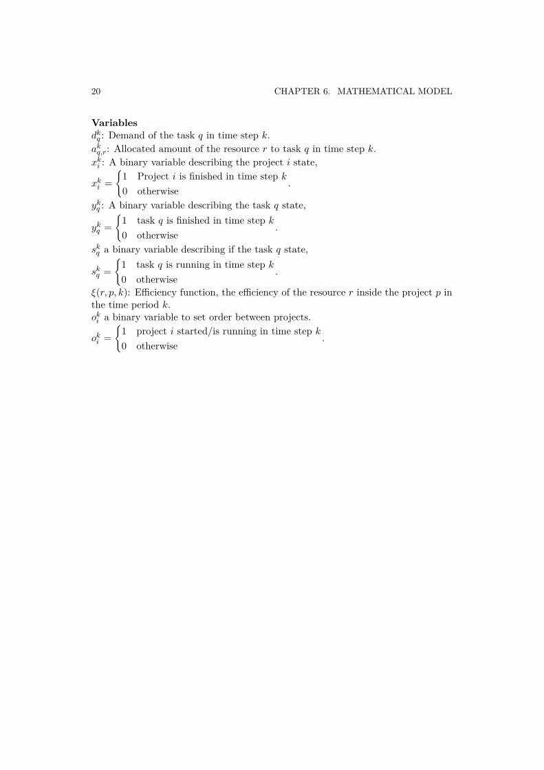
20 CHAPTER 6. MATHEMATICAL MODEL

Variablesdk

q : Demand of the task q in time step k.ak

q,r: Allocated amount of the resource r to task q in time step k.xk

i : A binary variable describing the project i state,

xki =

{1 Project i is finished in time step k0 otherwise

.

ykq : A binary variable describing the task q state,

ykq =

{1 task q is finished in time step k0 otherwise

.

skq a binary variable describing if the task q state,

skq =

{1 task q is running in time step k0 otherwise

.

ξ(r, p, k): Efficiency function, the efficiency of the resource r inside the project p inthe time period k.ok

i a binary variable to set order between projects.

oki =

{1 project i started/is running in time step k0 otherwise

.

6.1. NONLINEAR MODEL 21

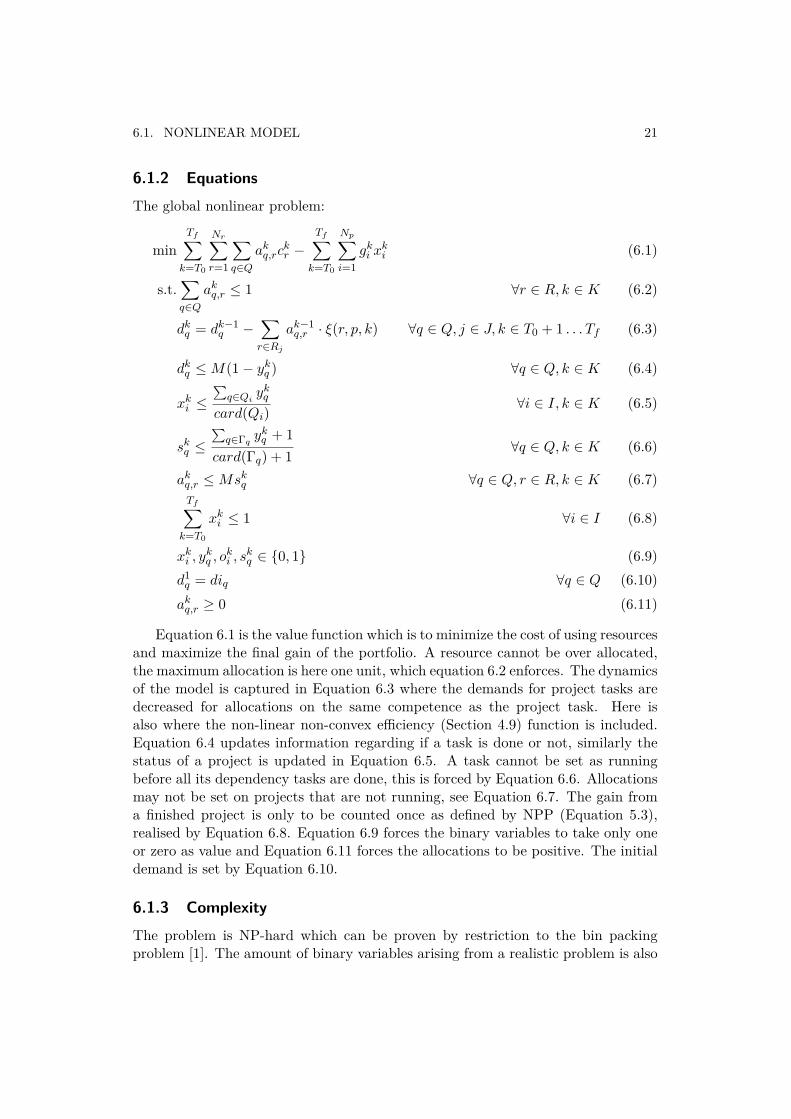
6.1.2 EquationsThe global nonlinear problem:

minTf∑

k=T0

Nr∑r=1

∑q∈Q

akq,rc

kr −

Tf∑k=T0

Np∑i=1

gki x

ki (6.1)

s.t.∑q∈Q

akq,r ≤ 1 ∀r ∈ R, k ∈ K (6.2)

dkq = dk−1

q −∑

r∈Rj

ak−1q,r · ξ(r, p, k) ∀q ∈ Q, j ∈ J, k ∈ T0 + 1 . . . Tf (6.3)

dkq ≤M(1− yk

q ) ∀q ∈ Q, k ∈ K (6.4)

xki ≤

∑q∈Qi

ykq

card(Qi)∀i ∈ I, k ∈ K (6.5)

skq ≤

∑q∈Γq

ykq + 1

card(Γq) + 1 ∀q ∈ Q, k ∈ K (6.6)

akq,r ≤Msk

q ∀q ∈ Q, r ∈ R, k ∈ K (6.7)Tf∑

k=T0

xki ≤ 1 ∀i ∈ I (6.8)

xki , y

kq , o

ki , s

kq ∈ {0, 1} (6.9)

d1q = diq ∀q ∈ Q (6.10)ak

q,r ≥ 0 (6.11)

Equation 6.1 is the value function which is to minimize the cost of using resourcesand maximize the final gain of the portfolio. A resource cannot be over allocated,the maximum allocation is here one unit, which equation 6.2 enforces. The dynamicsof the model is captured in Equation 6.3 where the demands for project tasks aredecreased for allocations on the same competence as the project task. Here isalso where the non-linear non-convex efficiency (Section 4.9) function is included.Equation 6.4 updates information regarding if a task is done or not, similarly thestatus of a project is updated in Equation 6.5. A task cannot be set as runningbefore all its dependency tasks are done, this is forced by Equation 6.6. Allocationsmay not be set on projects that are not running, see Equation 6.7. The gain froma finished project is only to be counted once as defined by NPP (Equation 5.3),realised by Equation 6.8. Equation 6.9 forces the binary variables to take only oneor zero as value and Equation 6.11 forces the allocations to be positive. The initialdemand is set by Equation 6.10.

6.1.3 ComplexityThe problem is NP-hard which can be proven by restriction to the bin packingproblem [1]. The amount of binary variables arising from a realistic problem is also


unmanageable, the problem is unsolvable for all but trivial problems.

6.2 Simplified model

By simplifying the stage-gate model so that a project is only one gate, but stillhaving one task per competence, the optimisation problem can be reduced. Asthere are no dependencies in this model all the tasks can be run in parallel, andthe amount of binary values is greatly reduced. To further reduce the complexitythe non convex efficiency function is reshaped to only include what the empiricalmethod indicates to be the most crucial part, learning. The learning will be includedas a penalty in the objective function, suppressing unnecessary moving of resourcesbetween projects. Non finished projects is included in the profit to give a resultcloser to what real steady state would give. To simplify even further the gain isindepend on project, but it is still discounted over time.

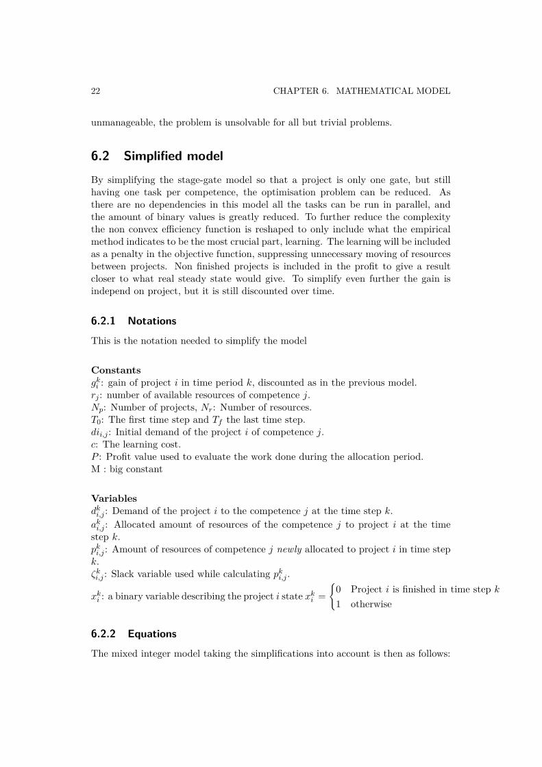
6.2.1 Notations

This is the notation needed to simplify the model

Constantsgk

i : gain of project i in time period k, discounted as in the previous model.rj : number of available resources of competence j.Np: Number of projects, Nr: Number of resources.T0: The first time step and Tf the last time step.dii,j : Initial demand of the project i of competence j.c: The learning cost.P : Profit value used to evaluate the work done during the allocation period.M : big constant

Variablesdk

i,j : Demand of the project i to the competence j at the time step k.ak

i,j : Allocated amount of resources of the competence j to project i at the timestep k.pk

i,j : Amount of resources of competence j newly allocated to project i in time stepk.ζk

i,j : Slack variable used while calculating pki,j .

xki : a binary variable describing the project i state xk

i ={

0 Project i is finished in time step k1 otherwise

6.2.2 Equations

The mixed integer model taking the simplifications into account is then as follows:

6.2. SIMPLIFIED MODEL 23

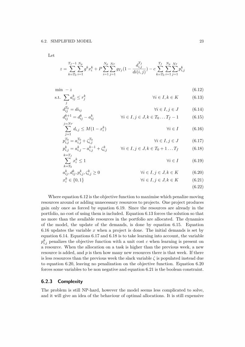
Let

z =Tf−1∑k=T0

Np∑i=1

gkxki + P

Np∑i=1

Nr∑j=1

gTf(1−

dTf

i,j

di(i, j))− cTf∑

k=T0

Np∑i=1

Nr∑j=1

pki,j

min − z (6.12)s.t.

∑j

akij ≤ rk

j ∀i ∈ I, k ∈ K (6.13)

dT0ij = diij ∀i ∈ I, j ∈ J (6.14)dk+1

ij = dkij − ak

ij ∀i ∈ I, j ∈ J, k ∈ T0 . . . Tf − 1 (6.15)j=Nr∑j=1

di,j ≤M(1− xki ) ∀i ∈ I (6.16)

pT0i,j = aT0

i,j + ζT0i,j ∀i ∈ I, j ∈ J (6.17)

pki,j = ak

i,j − ak−1i,j + ζk

i,j ∀i ∈ I, j ∈ J, k ∈ T0 + 1 . . . Tf (6.18)k=Tf∑k=T0

xki ≤ 1 ∀i ∈ I (6.19)

akij , d

kij , p

ki,j , ζ

ki,j ≥ 0 ∀i ∈ I, j ∈ J, k ∈ K (6.20)

xki ∈ {0, 1} ∀i ∈ I, j ∈ J, k ∈ K (6.21)

(6.22)

Where equation 6.12 is the objective function to maximise which penalize movingresources around or adding unnecessary resources to projects. One project producesgain only once as forced by equation 6.19. Since the resources are already in theportfolio, no cost of using them is included. Equation 6.13 forces the solution so thatno more than the available resources in the portfolio are allocated. The dynamicsof the model, the update of the demands, is done by equation 6.15. Equation6.16 updates the variable x when a project is done. The initial demands is set byequation 6.14. Equations 6.17 and 6.18 is to take learning into account, the variablepk

i,j penalizes the objective function with a unit cost c when learning is present ona resource. When the allocation on a task is higher than the previous week, a newresource is added, and p is then how many new resources there is that week. If thereis less resources than the previous week the slack variable ζ is populated instead dueto equation 6.20, leaving no penalization on the objective function. Equation 6.20forces some variables to be non negative and equation 6.21 is the boolean constraint.

6.2.3 ComplexityThe problem is still NP-hard, however the model seems less complicated to solve,and it will give an idea of the behaviour of optimal allocations. It is still expensive


and will prove solvable only for portfolios with low number of projects, competencesand weeks.

Empirical model

Since the full problem is unsolvable with realistic computer power another way toexamine the problem is necessary, and for this a simulation framework was producedand implemented. The simulation framework enables testing of different resourceallocation strategies to see how they influence the value of a certain portfolio ofprojects and resources. As the simulation time is short, a matter of seconds, theeffects of changing nonlinearity functions and other model parameters can be inves-tigated.

7.1 FeaturesNon-linear efficiency used in simulation framework:

• Knowledge learning.

• Knowledge loss.

• Project task resource ramping.

• Multiple resource per project task.

• Multiple project task per resource.

The corresponding efficiency contributions can be seen in Section 4.9.

7.2 OutputThe main analysed output from a simulation is the Net Present Profit (NPP) forthe portfolio, as discussed in Section 5.3.

7.3 Steady stateIt is important to properly handle start and end time and its effect on NPP, seeSection 5.2. When the simulation starts no project in the portfolio is started andthey all start in the same stage, as the stages are very similar in the differentprojects this creates unrealistic bottlenecks. The chosen approach to remove these

25

26 CHAPTER 7. EMPIRICAL MODEL

bottlenecks is to run the simulation on the portfolio until the running projects areno longer in phase and thus have a realistic start for the NPP calculation, withsome projects already started and running; this is called steady state. The amountof steps to run before calculating NPP is called pre-run. A project that is notfinished always has a NPP, which is defined to be the portion of how much workthat has been produced in respect to the initial demand and its expected gain atthe extrapolated finish time from the current work per time step ratio, see Equation(5.4).

7.4 Portfolio execution strategies

To examine the behaviour of a full model in different scenarios different strategieswere implemented into the simulation. A strategy is responsible to set allocation ofresources to projects in a fixed time step, based on the current state of the portfolio.As one of the decision variables in portfolio execution is the number of projects runsimultaneously this appears as an input variable in all strategies. Some strategiesmake a distinction between prioritized and running projects, which means that therecan be projects running that is not normally being allocated but instead is allocatedresources not used by the prioritized projects (these are called slack projects).

7.4.1 Equal sharing

The available resources is shared equally between the prioritized projects, regardlessof their sizes and the stage that they are in. Resources not usable in the prioritizedprojects can be allocated to various slack projects.

7.4.2 Equal sharing, prioritise running

The equal share of the available resources is calculated. Then iterating through theprojects in the priority order, the project receives the equal share if it is higher thanthe present allocation. This might make it so that some projects does not get theirequal share, but the first projects in priority order will get a higher allocation.

7.4.3 Execute allocations

In order to reduce complexity in designing strategies they do not, in the phase ofcalculation desired allocations for all project, consider the individual resources butinstead only look at the amount of work that has to be done. A function then existsto move the individual resources to fulfil these allocations. If the allocations for theresources are done badly it will have a huge impact on efficiency and will distortthe results. To solve this problem a unified way to go from allocations of units ofresources to individual resources is used. There are then multiple variants of thisfunction to choose the resource to fill a allocation on a task.

7.5. WEAKNESSES 27

Resource dividing allocation

When resources are taken arbitrarily from available resources in the portfolio withno sensible prioritization the resources will end up with many allocations. They willstart to split into small allocations on many projects which will drastically reducethe overall efficiency of the resources.

No limits resource queueing allocation

The way resources are chosen to fill a required allocation is as following, take fromfree resources in the following order:

• Already assigned to the project.

• Last worked on project.

• Allocated to least number of projects.

• Low availability left.

If there are not enough available resources it take as much as possible. This willstill split resources, but not as much as the Resource dividing allocation does.

Resource queueing allocation

Using the same queuing principle as no limits resource queueing allocation butadding a vital limit to the allocations. By setting limits on the minimum alloca-tion from a resource to allocate, by taking all that is left from that resource theunnecessary splitting of resources is suppressed to a minimum.

7.5 WeaknessesIf the strategy makes good decisions on what a project should have as allocationsthey can easily be diminished by bad choices of resources for those allocations, whichcan distort the results. A resource might be split too much and working on manyprojects and thus become inefficient on all those projects. Or one might reallocatea resource from a project and later fill that spot with another resource that haveno knowledge at the project, thus introducing unnecessary lead time.

Results

8.1 Analytical

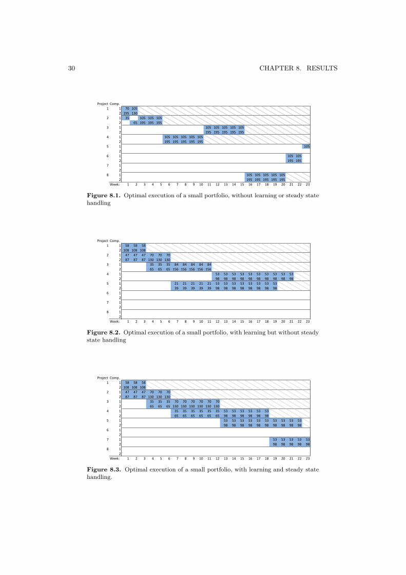
In order to study the behaviour of an optimal solution a small linear portfolioexecution problem was implemented using the GAMS (General Algebraic ModelingSystem) modelling language. To solve these models the computer solver SNOPT(see [10]) was used. Different problems were solved, all using the same portfolio; theinitial problem was the simplest possible linear execution, and in turn the effect oflearning and that of steady state were added. Description of the portfolio used canbe found in Appendix A.1, most notable is that project 1 and 2 are both partiallydone at the beginning of the period. From the solution it is possible to extract ageneral trend in how projects are allocated, and what effect learning has.

In Figure 8.1 the results from solving the problem defined in Section 6.2, withoutlearning or cost of resource usage, can be seen. The figure presents the allocationof resources per project, competence and week. The gray diagonal lines representsfinished projects. Notably large numbers are used in order to avoid rounding errorsthat might otherwise influence the solution in the particular solver used. In thissolution the main trend is to prioritize only one single project, and if all resourcescan not be used in that project transfer them to the next project to be started.

When a simplified version of learning is added, described by Equations 6.17and 6.18, the allocations change and can now be seen in Figure 8.2. Learning isimplemented as penalty cost, instead of a lowered efficiency, for implementationreasons. Because of the learning the results now differ, and instead prioritises twoprojects. Notable is that no allocations are made in the end of the period, as onlyfinished projects are rewarded.

With steady state considered (see Section 5.2) the objective function changesfurther, and now gives gain for projects that are partially finished at the end of therun period. With this the solution, presented in Figure 8.3, contains allocations inprojects that does not finish during the period.

8.2 Empirical

With the simulation framework described in Chapter 7 different strategies can berun with a set of different settings in order to give an understanding of the be-

29

30 CHAPTER 8. RESULTS

Project Comp.1 1 70 105

2 195 1302 1 35 105 105 105

2 65 195 195 1953 1 105 105 105 105 105

2 195 195 195 195 1954 1 105 105 105 105 105

2 195 195 195 195 1955 1 105

26 1 105 105

2 195 1957 1

28 1 105 105 105 105 105

2 195 195 195 195 195Week: 1 2 3 4 5 6 7 8 9 10 11 12 13 14 15 16 17 18 19 20 21 22 23

Figure 8.1. Optimal execution of a small portfolio, without learning or steady statehandling

Project Comp.1 1 58 58 58

2 108 108 1082 1 47 47 47 70 70 70

2 87 87 87 130 130 1303 1 35 35 35 84 84 84 84 84

2 65 65 65 156 156 156 156 1564 1 53 53 53 53 53 53 53 53 53 53

2 98 98 98 98 98 98 98 98 98 985 1 21 21 21 21 21 53 53 53 53 53 53 53 53

2 39 39 39 39 39 98 98 98 98 98 98 98 986 1

27 1

28 1

2Week: 1 2 3 4 5 6 7 8 9 10 11 12 13 14 15 16 17 18 19 20 21 22 23

Figure 8.2. Optimal execution of a small portfolio, with learning but without steadystate handling

Project Comp.1 1 58 58 58

2 108 108 1082 1 47 47 47 70 70 70

2 87 87 87 130 130 1303 1 35 35 35 70 70 70 70 70 70

2 65 65 65 130 130 130 130 130 1304 1 35 35 35 35 35 35 53 53 53 53 53 53

2 65 65 65 65 65 65 98 98 98 98 98 985 1 53 53 53 53 53 53 53 53 53 53

2 98 98 98 98 98 98 98 98 98 986 1

27 1 53 53 53 53 53

2 98 98 98 98 988 1

2Week: 1 2 3 4 5 6 7 8 9 10 11 12 13 14 15 16 17 18 19 20 21 22 23

Figure 8.3. Optimal execution of a small portfolio, with learning and steady statehandling.

8.2. EMPIRICAL 31

0 20 40 60 80 1006

8

10

12

14

16

18

20

22

nr prioritized projects

Accu

mu

late

d g

ain

Equal sharing, prioritise running

Equal sharing

Figure 8.4. Equal sharing and Equal sharing, prioritise running

haviour of more complex portfolios, impossible to solve analytically. The mainparameters varied in the different simulations with different strategies are the num-ber of projects run by the R&D department. All simulations are run using a MonteCarlo method, they are run multiple times with randomly generated portfolios togenerate approximate average values and confidence intervals.

8.2.1 Portfolio investigated

The portfolio used consists of 15 competences and 600 projects with an average of1000 man week demands, 300 resources. Each project follows the stage gate modelwith six stages. The amount of each resource is proportional to the mean demandper competence. See Appendix A.1.

8.2.2 Portfolio execution strategies

The portfolio execution strategy Equal sharing, prioritise running, performs betterthan Equal sharing over the interesting simulation interval with the described port-folio, see Figure 8.4. Therefore the simulations was conducted using Equal sharing,prioritise running.

8.2.3 Steady-state effects

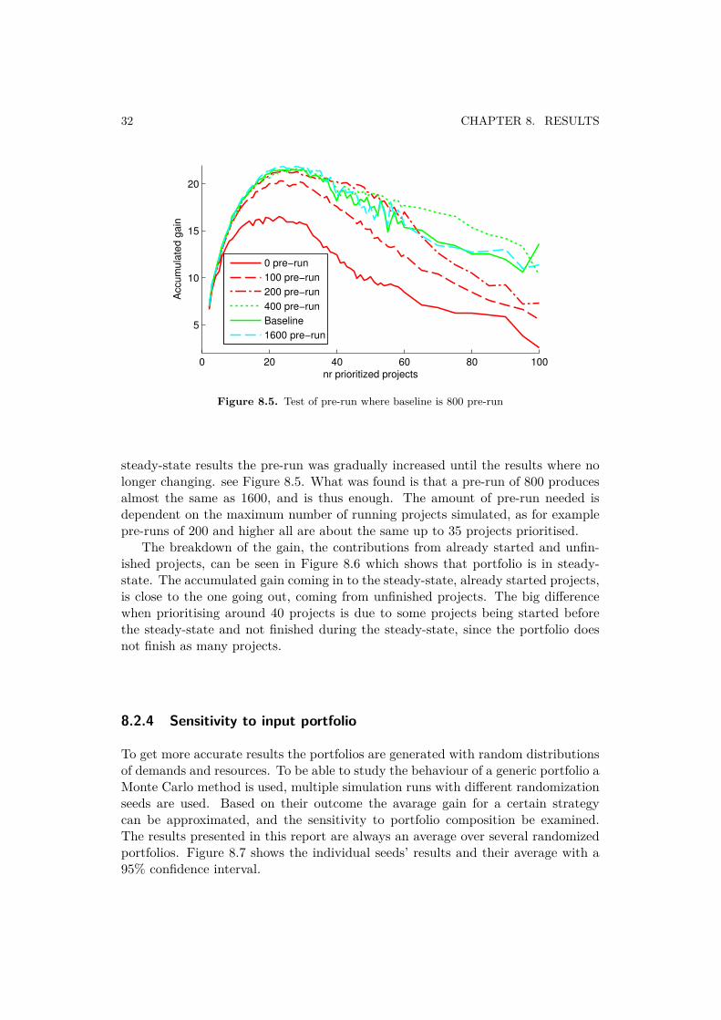
As described in Section 7.3 the steady state has an big impact on the results.The definition of steady state is clear, however finding a large-enough pre-run (seeSection 7.3) to produce this is not trivial. An infinite pre-run is desired but notfeasible. Since a long pre-run takes much computational time the shortest butsufficiently long pre-run is desired. To find the minimum pre-run required to produce


0 20 40 60 80 100

5

10

15

20


Accu

mu

late

d g

ain

0 pre−run

100 pre−run

200 pre−run

400 pre−run

Baseline

1600 pre−run

Figure 8.5. Test of pre-run where baseline is 800 pre-run

steady-state results the pre-run was gradually increased until the results where nolonger changing. see Figure 8.5. What was found is that a pre-run of 800 producesalmost the same as 1600, and is thus enough. The amount of pre-run needed isdependent on the maximum number of running projects simulated, as for examplepre-runs of 200 and higher all are about the same up to 35 projects prioritised.

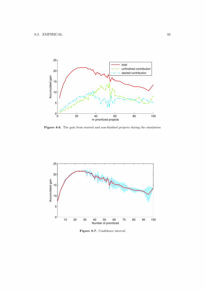
The breakdown of the gain, the contributions from already started and unfin-ished projects, can be seen in Figure 8.6 which shows that portfolio is in steady-state. The accumulated gain coming in to the steady-state, already started projects,is close to the one going out, coming from unfinished projects. The big differencewhen prioritising around 40 projects is due to some projects being started beforethe steady-state and not finished during the steady-state, since the portfolio doesnot finish as many projects.

8.2.4 Sensitivity to input portfolio

To get more accurate results the portfolios are generated with random distributionsof demands and resources. To be able to study the behaviour of a generic portfolio aMonte Carlo method is used, multiple simulation runs with different randomizationseeds are used. Based on their outcome the avarage gain for a certain strategycan be approximated, and the sensitivity to portfolio composition be examined.The results presented in this report are always an average over several randomizedportfolios. Figure 8.7 shows the individual seeds’ results and their average with a95% confidence interval.

8.2. EMPIRICAL 33

0 20 40 60 80 1000

5

10

15

20

25


Accu

mu

late

d g

ain

total

unfinished contribution

started contribution

Figure 8.6. The gain from started and non-finished projects during the simulation

10 20 30 40 50 60 70 80 90 1000

5

10

15

20

25

Number of prioritized

Accu

mu

late

d g

ain

Figure 8.7. Confidence interval


Resources150 225 300 375 450

Totalw

ork 500 21 28 35 45 56

750 16 22 29 37 431000 15 20 26 31 381250 14 19 24 29 341500 13 18 23 26 32

Table 8.1. Optimal nr projects to prioritize, total work in man weeks

Comp 2 3 4 5 6 7 8 9 10Projects 21 36 35 32 31 30 28 28 28

Comp 11 12 13 14 15 16 17 18 19 20Projects 27 27 28 27 26 25 25 24 24 25

Table 8.2. Optimal nr projects to prioritize, changing the amount of competenceswith constant portfolio size

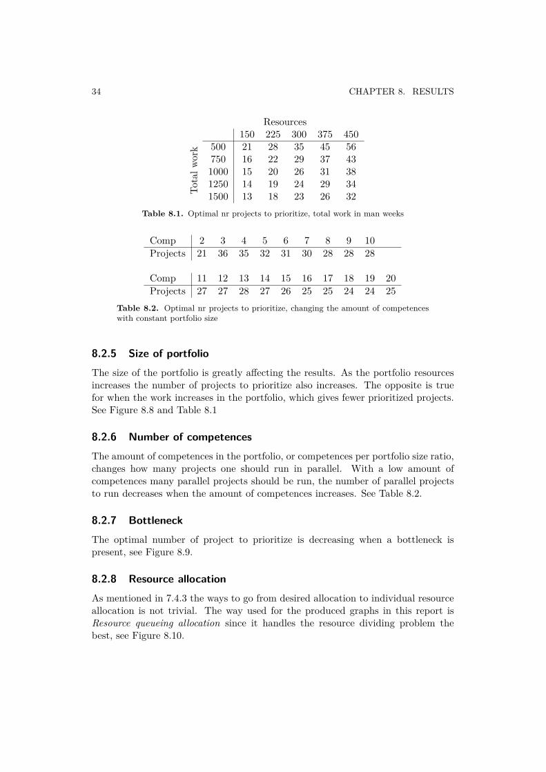
8.2.5 Size of portfolioThe size of the portfolio is greatly affecting the results. As the portfolio resourcesincreases the number of projects to prioritize also increases. The opposite is truefor when the work increases in the portfolio, which gives fewer prioritized projects.See Figure 8.8 and Table 8.1

8.2.6 Number of competencesThe amount of competences in the portfolio, or competences per portfolio size ratio,changes how many projects one should run in parallel. With a low amount ofcompetences many parallel projects should be run, the number of parallel projectsto run decreases when the amount of competences increases. See Table 8.2.

8.2.7 BottleneckThe optimal number of project to prioritize is decreasing when a bottleneck ispresent, see Figure 8.9.

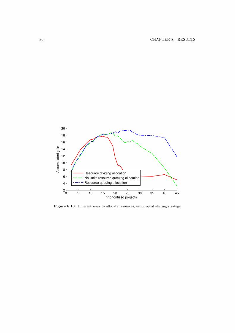
8.2.8 Resource allocationAs mentioned in 7.4.3 the ways to go from desired allocation to individual resourceallocation is not trivial. The way used for the produced graphs in this report isResource queueing allocation since it handles the resource dividing problem thebest, see Figure 8.10.

8.2. EMPIRICAL 35

0 20 40 60 80 1000

10

20

30

40


Accu

mu

late

d g

ain

Baseline

Double resources and work

Half resources and work

0 20 40 60 80 1000

10

20

30

40


Accu

mu

late

d g

ain

Baseline

Double resources

Half resources

0 20 40 60 80 1000

10

20

30

40


Accu

mu

late

d g

ain

Baseline

Double work

Half work

Figure 8.8. Different sizes of portfolios, results scaled

0 20 40 60 80 1004

6

8

10

12

14

16

18

20

22


Accu

mu

late

d g

ain

Baseline

Competence nr 0

Competence nr 9

Competence nr 13

Figure 8.9. Bottleneck of 75% on different competences and baseline


0 5 10 15 20 25 30 35 40 452

4

6

8

10

12

14

16

18

20


Accu

mu

late

d g

ain

Resource dividing allocation

No limits resource queuing allocation

Resource queuing allocation

Figure 8.10. Different ways to allocate resources, using equal sharing strategy

Discussion

9.1 Analytical

The analytical solution of the simplified problem presented in Section 6.2 givesinteresting information about the behaviour of the optimal solution. The resultsare interesting not only in their own but also as a motivation for the chosen way ofrepresenting the problem when simulating portfolio executions.

The general trend that can be seen is that a limited number of projects are runin parallel, with stepwise constant allocations only changing when other projects arefinished. The number of prioritized projects are changed with the cost of switching,where a higher cost of switching leads to more projects running in parallel.

However the results from this part should be looked at knowing the limitationsof the model that produced them. Several severe limitations have been made inthe simplified model. The first one is the absence of the stage-gate model projectdescription, it is instead replaced by a linear demand execution. This mainly takesaway the desire to run several projects in different stages in order to reduce thebottlenecking several projects in the same stage produces. The linear demand ex-ecution also creates problem when bottlenecking occurs, as one demand can befinished without the others being started.

The other big simplification is in the efficiency functions, where only learning isconsidered, and only in a simplified form. As learning is introduced as a cost in theobjective function instead of as an increase in the required demand for a project,the project execution time is shorter than it should, especially for short projectexecution times.

Viewed in the light of its shortcomings the model still gives results that areinteresting to study, the general trend of allocating to a limited number of projectsand reallocating only when other projects are finished are both interesting results.In a real-world environment with delays, unknown demands and different projectstages the results become less usable.

Future study in this area would be to expand the simplified model to supportmultiple stages. With access to a solver on a more powerful computer that problemwould be solvable in reasonable time, and give more definitive answers on how to runrealistic projects optimally. Another area of the model is the treatment of learning,a function closer to the desired behaviour that allows for realistic solution timeswould increase the quality of the results.

37

38 CHAPTER 9. DISCUSSION

9.2 EmpiricalThe results from the simulation of the portfolio execution strategies is in line withand strengthens the findings in the analytical analysis, that there is an numberof running projects that is the optimal for profit, and that starting more projectsafter this point is counter-productive. That number is of high interest, however it ishard to find a rule of what it should be; the simulations indicate that it is stronglydependent on the size and composition of the portfolio, and it would also dependon the portfolio execution strategy used. The two portfolio execution strategiestested, equal sharing and equal sharing, prioritise running, are not enough to drawconclusions about where that point lies even for the tested portfolio, even when usingrealistic heuristics. The simulations does however produce an order of magnitudefor this number and behaviour of the value.

As pointed out in Section 7.5 there is no certainty that the results from thesimulator is representative of the portfolio execution strategies it is set to investi-gate, since the implementation of strategies is complex and small changes in theimplementation can have big effects.

The superior results of Equal sharing, prioritise running over Equal sharingmight indicate that prioritising to finish started tasks, not removing previous allo-cations, is the way to go, or it might be due to the fact that Equal sharing loosesextra efficiency since more resources are moved around.

The efficiency functions used are not validated by extensive research, but ratherdeduced from the extensive knowledge accumulated in the companies Atlas Copcoand Level 21 Management. The exact shape of these function might therefore besubject to debate, but as long as the shapes of the functions are agreed on thegeneral trends of the solutions should remain the same.

Since there is no cost on using resources the portfolio execution strategies willuse as much resources as possible and thus always have near full utilization. Asthere is no cost of being allocated to a project nor a penalty for going directly fromone project to another, this should thus not impact the execution of the portfolionegatively.

The extensive results achieved in the empirical study indicates that this kind ofsimulation would be worth further investigation. As it simulates the portfolio exe-cution with much higher level of detail than the mathematical models, it is possibleto study more complex scenarios. The main area of improvement would be furtherresearch and testing of portfolio execution strategies, both to find more realisticrepresentation of strategies currently used in companies to serve as a baseline andto formulate other heuristic strategies that brings the results closer to the real op-tima. Such strategies could also provide more information such as the impact onprofits from maximizing utilization.

Conclusion

With both the analytical and the empirical studies of the resource allocation prob-lem three main results can be extracted from the accumulated knowledge and re-sults.

The first one concerns the problem formulation and the possibility for optimisa-tion. That the allocation problem is NP hard had been proved before the work onthis project began [1]; in this project it was further found that for a realistic mod-elling of execution of projects in a full R&D department the amount of variablesbecome unmanageable. In conclusion the problem is too big to solve analyticallyand to complex to draw final conclusions about optimality using heuristics.

The second major result is that every model points to the existence of an optimalvalue for the number of project to run. However the overall complexity to allocateresources to projects indicates that the point will be hard to find, it is only clearthat a too big or too small number of running projects results in a notably lowerprofit. The answer to how many project to run in parallel is unanswered but someof its depending variables have been found; it is highly dependent of the size of theportfolio and the ways to allocate the resources.

This leads to the third main result, that the way resources are allocated toprojects are of great importance, in the empirical studies the allocation strategiesimpacted the results massively. Keeping track of past allocations and avoiding tosplit a resource unnecessarily had great impact. This seems to mostly be a problemfor numbers of running projects, but also the optimal value is affected and pusheddown by a bad allocation strategy.

39

Bibliography

[1] Senay Solaka & John-Paul B. Clarke & Ellis L. Johnsonc & Earl R. Barnes.Optimization of r&d project portfolios under endogenous uncertainty. EuropeanJournal of Operational Research, May 2010.

[2] Matt Basset. Assigning projects-to optimize the utilization of employees’ timeand expertise. Computers and Chemical Engineering, 2000.

[3] Robert G. Cooper. Stage-gate systems: A new tool for managing new products.Business Horizon, May-June 1990.

[4] N. Archer F. Ghasemzadeh and P. Iyogun. A zero-one model for project portfo-lio selection and scheduling. The Journal of the Operational Research Society,July 1999.

[5] Antonella Certa & Mario Enea & Giacomo Galante & Concetta Manuela LaFata. Multi-objective human resources allocation in r&d projects planning.International Journal of Production Research, July 2009.

[6] Dennis S. Kira & Martin I. Kusy & David H. Murray & Barbara J. Goranson.A specific decision support system (sdss) to develop an optimal project port-folio mix under uncertainty. IEEE TRANSACTIONS ON ENGINEERINGMANAGEMENT, August 1990.

[7] Frederick S. Hillerman and Gerald J. Lieberman. Introduction to OperationsResearch. McGraw-Hill, New York, ninth international edition edition, 2010.

[8] Ulf Högman and Hans Johannesson. Applying stage-gate processes to technol-ogy development - experience from six hardware-orientated companies. Journalof Engineering and Technology Management, 2013.

[9] Elhabib Moustaid. Optimal project portfolio execution - computer implemen-tation of models and simulation framework. Master Thesis Report.

[10] Walter Murray Philip E. Gill and Michael A. Saunders. Snopt: An sqp al-gorithm for large-scale constrained optimization. Society for Industrial andApplied Mathematics, 2005.

41

Appendix

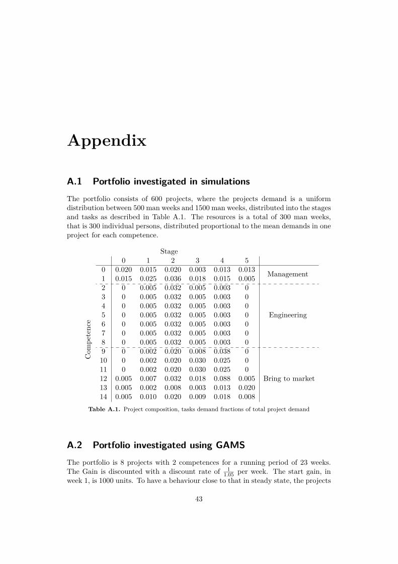
A.1 Portfolio investigated in simulationsThe portfolio consists of 600 projects, where the projects demand is a uniformdistribution between 500 man weeks and 1500 man weeks, distributed into the stagesand tasks as described in Table A.1. The resources is a total of 300 man weeks,that is 300 individual persons, distributed proportional to the mean demands in oneproject for each competence.

Stage0 1 2 3 4 5

0 0.020 0.015 0.020 0.003 0.013 0.013 Management1 0.015 0.025 0.036 0.018 0.015 0.0052 0 0.005 0.032 0.005 0.003 0

Engineering

3 0 0.005 0.032 0.005 0.003 04 0 0.005 0.032 0.005 0.003 05 0 0.005 0.032 0.005 0.003 0

Com

petenc

e 6 0 0.005 0.032 0.005 0.003 07 0 0.005 0.032 0.005 0.003 08 0 0.005 0.032 0.005 0.003 09 0 0.002 0.020 0.008 0.038 0

Bring to market

10 0 0.002 0.020 0.030 0.025 011 0 0.002 0.020 0.030 0.025 012 0.005 0.007 0.032 0.018 0.088 0.00513 0.005 0.002 0.008 0.003 0.013 0.02014 0.005 0.010 0.020 0.009 0.018 0.008

Table A.1. Project composition, tasks demand fractions of total project demand

A.2 Portfolio investigated using GAMSThe portfolio is 8 projects with 2 competences for a running period of 23 weeks.The Gain is discounted with a discount rate of 1

1.05 per week. The start gain, inweek 1, is 1000 units. To have a behaviour close to that in steady state, the projects

43

44 APPENDIX A. APPENDIX

are in different phases of the demands, other than that they are similar. The initialdemands are as following:

Demand P 1 P 2 P 3 P 4 P 5 P 6 P 7 P 8Competence 1 175 350 525 525 525 525 525 525Competence 2 325 650 975 975 975 975 975 975

Table A.2. Table of demands

The amount of available resources are directly proportional to the demands,with a total available 300 man work weeks, consisting of 105 man work weeks forcompetence 1 and 195 for competence 2.

TRITA-MAT-E 2014:04 ISRN-KTH/MAT/E—14/04-SE

www.kth.se

optimal project portfolio execution -...

Documents