Optimal regions for congested

transport

Giuseppe Buttazzo

Dipartimento di Matematica

Universita di Pisa

buttazzo@dm.unipi.it

http://cvgmt.sns.it

Workshop “Optimal Transport in the Applied Sciences”Johann Radon Institute (RICAM)

Linz, December 8–12, 2014

Joint work with:

Guillaume Carlier - Paris DauphineSerena Guarino - University of Pisa

Math. Model. Numer. Anal. (M2AN),(to appear)

available at:http://cvgmt.sns.it

arxiv.org

1

We consider a geographical region Ω in which

two densities f+ and f− are given; for in-

stance we may think f+ is the distribution

of residents in Ω and f− the distribution of

working places. We assume∫Ωf+ dx =

∫Ωf− dx.

We also assume that the transport in Ω is

congested and that the congestion function

is given by a convex nonnegative superlinear

function H.

2

It is known that in this case the traffic flux σ,

in the stationary regime, reduces to a min-

imization problem of the form (Beckmann

model)

min ∫

ΩH(σ) dx : σ ∈ Γf

where

Γf =− div σ = f in Ω, σ · n = 0 on ∂Ω

,

being f = f+− f−. See for instance Brasco-

Carlier, Carlier-Jimenez-Santambrogio for de-

tails on the model.

3

The pure Monge’s problem corresponds to

H(s) = |s| in which no congestion occurs,

and the congestion effect is higher for larger

functions H.

In some cases, the transportation cost can

be +∞ if the source and target measures f+

and f− are singular; for instance, if H has a

quadratic growth, in order to have a finite

cost it is necessary that the signed measure

f = f+ − f− be in the dual Sobolev space

H−1.

4

Our goal is to reduce the congestion acting

on a suitable region C which has to be deter-

mined. More precisely, two congestion func-

tions H1 and H2 are given, with H1 ≤ H2,

and the goal is to find an optimal region

C ⊂ Ω where we enforce a traffic conges-

tion reduction.

Since reducing the congestion in C is costly,

a penalization term m(C) is added, to de-

scribe the cost of the improvement, then pe-

nalizing too large low-congestion regions.

5

For every region C we then consider the shape

function

F (C) = min ∫

Ω\CH2(σ) dx+

∫CH1(σ) dx : σ ∈ Γf

and so the optimal design of the low-congestion

region amounts to the minimization problem

minF (C) +m(C) : C ⊂ Ω

.

Much of the analysis below depends on the

penalization function m(C).

6

The case m(C) = kPer(C)

Theorem For every k > 0 there exists anoptimal solution Copt.

Indeed, a minimizing sequence Cn has a uni-formly bounded perimeter and so we may as-sume that Cn tends strongly in L1 to someset C. The perimeter is L1-lower semicon-tinuous; moreover, the optimal σn ∈ Γf pro-viding the value

F (Cn) =∫

Ω\CnH2(σn) dx+

∫CnH1(σn) dx

7

are weakly L1 compact, due to the super-

linearity of the congestion functions (de La

Vallee Poussin theorem). The conclusion

now follows from the strong-weak lower semi-

continuity theorem for integral functionals.

The necessary conditions of optimality are:

σ =

∇H∗1(∇uint) in C

∇H∗2(∇uext) in Ω \ C

where uint and uext solve the PDEs

8

−div(∇H∗1(∇uint)

)= f in C

∇H∗1(∇uint) · ν = 0 on ∂Ω ∩ C−div(∇H∗2(∇uext)

)= f in Ω \ C

∇H∗2(∇uext) · ν = 0 on ∂Ω ∩ (Ω \ C)

with the transmission condition across ∂C

∇H∗1(∇uint)−∇H∗2(∇uext)·νC = 0 on ∂C∩Ω.

Performing the shape derivative on ∂C we

also obtain on ∂C ∩Ω

9

H2

(∇H∗2(∇uext)

)−H1

(∇H∗2(∇uext)

)≤ kHC

≤ H2

(∇H∗1(∇uint)

)−H1

(∇H∗1(∇uint)

).

where HC is the mean curvature on ∂C. Since

H1 ≤ H2 this gives that HC ≥ 0.

If d = 2 and Ω is convex, replacing C by

its convex hull diminishes the perimeter and

also the congestion cost, so the optimal C

are convex.

10

The case m(C) = k|C|

Passing from sets C to density functions θ(x) ∈[0,1] we obtain the relaxed formulation

minσ,θ

∫Ω

(θH1(σ) + (1− θ)H2(σ) + kθ

)dx

.

The minimization with respect to θ is straight-forward and the optimal θ is

θ = 1H1(σ)+k<H2(σ),

which reduces the problem to

minσ

∫ΩH2(σ) ∧

(H1(σ) + k

)dx.

11

Since the function H = H2 ∧ (H1 + k) is not

convex, a further relaxation gives finally the

problem

minσ

∫ΩH∗∗(σ) dx.

If σ is a solution, we have

• if H∗∗(σ) = H2(σ) we take θ = 0, that is no

improvement for low congestion is needed;

• if H∗∗(σ) = H1(σ) + k we take θ = 1, that

is in this region we have to spend a lot to

improve the congestion;

• if H∗∗(σ) < H(σ) we have to spend re-

sources proportionally to θ(x) ∈]0,1[.

12

If H1 and H2 only depend on |σ| we get

θ(x) =

0 if |σ| ≤ r1|σ|−r1r2−r1

if r1 < |σ| < r2

1 if |σ| ≥ r2

where r1 and r2 can be explicitly computed

from H1 and H2:

r1 = max. solution of H∗∗(r) = H2(r)

r2 = min. solution of H∗∗(r) = H1(r) + k.

Some numerical computations can be made

when H1 and H2 are quadratic.

13

The problem in this case is similar to thetwo-phase shape optimization problem, forwhich we refer to the book by Allaire [Springer2001]. We take:

H1(σ) = a|σ|2, H2(σ) = b|σ|2 with a < b.

Then we have

H∗(ξ) =ξ2

4b∨(ξ2

4a− k

)and we simply have to solve the elliptic prob-lem (with Neumann b.c.)

min ∫

Ω

(H∗(∇u)− fu

)dx

.

14

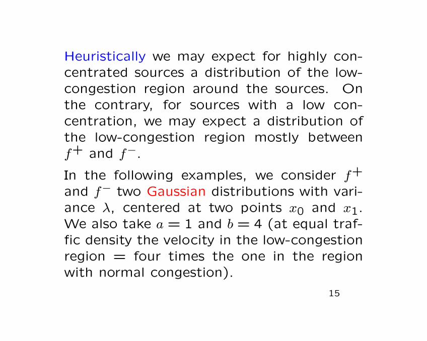
Heuristically we may expect for highly con-centrated sources a distribution of the low-congestion region around the sources. Onthe contrary, for sources with a low con-centration, we may expect a distribution ofthe low-congestion region mostly betweenf+ and f−.

In the following examples, we consider f+

and f− two Gaussian distributions with vari-ance λ, centered at two points x0 and x1.We also take a = 1 and b = 4 (at equal traf-fic density the velocity in the low-congestionregion = four times the one in the regionwith normal congestion).

15

Gaussian sources (left) with variance λ =

0.02; plot of θ (right) using the penalization

parameter k = 0.4. Computations made by

Serena Guarino using FreeFem.

16

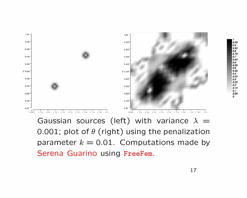
Gaussian sources (left) with variance λ =

0.001; plot of θ (right) using the penalization

parameter k = 0.01. Computations made by

Serena Guarino using FreeFem.

17

A free boundary problem arising in PDEoptimization(Joint work with E. Oudet and B. Velichkov)

In the problem above assume we have a groundcongestion given by the function H(σ) =12|σ|

2 and that, investing an amount θ ofresources produces a lower congestion like

12(1+θ)|σ|

2. We have then the problem

sup∫D θ dx=m

infu∈H1

0(D)

∫D

(1 + θ

2|∇u|2 − fu

)dx

where the total amount of resources to spendis fixed.

18

In this case the Dirichlet zero boundary con-dition means that we want to transport themass f(x) dx to the boundary of D. A similarsituation occurs when we have the Neumannboundary condition but for a right-hand sidef with zero mean.

Interchanging the sup and the inf above gives

infu∈H1

0(D)sup∫

D θ dx=m

∫D

(1 + θ

2|∇u|2 − fu

)dx

and now the sup with respect to θ, for a fixedu, is easy to compute and we end up with

minu∈H1

0(D)

1

2

∫D|∇u|2 dx+

m

2‖∇u‖2∞−

∫Dfu dx

.

19

The existence of a solution u for this lastproblem is straightforward and, by strict con-vexity it is also unique. In order to solve theinitial optimization problem the questions areto recover the optimal function θ from u andto describe the boundary of the free set

Ω =|∇u| < ‖∇u‖∞

.

• An easier case is the torsion problem, wheref = 1. Indeed, we may show the equivalencewith the obstacle problem

min ∫

D

(1

2|∇u|2−u

)dx : u ∈ H1

0(D), u(x) ≤ kd(x)

20

where d(x) is the distance function from ∂D

and k = ‖∇u‖∞. In this case the free set

Ω =|∇u| < ‖∇u‖∞

coincides with the

complement|u| < kd

of the contact set.

Since the solution uk of the obstacle prob-

lem is continuous, the free set Ω is open.

• Still in the torsion case, by the equivalence

with the obstacle problem, we may conclude

that the free boundary ∂Ω is C1,α up to a

singular set of zero Hausdorff d−1 measure.

21

• Still in the torsion case, the cut locus of D,that is the set where the distance functiond is singular, is fully contained into the freeset Ω.

• When f = 1 and D is the unit ball, theexplicit expression of θ can be computed:

θ(r) =[r

am− 1

]+where am is a suitable constant.

• The previous argument cannot be repeatedfor a general right-hand side f .

22

• A much easier case is when the constraint

on θ is of Lp type (p > 1)θ ≥ 0,

∫Dθp dx ≤ m

.

In this case the optimal θ is given by (q = p′)

θ = m1/p|∇u|2/(p−1)( ∫

D|∇u|2q dx

)−1/p

where u solves the minimum problem for

1

2

∫D|∇u|2 dx+

m1/p

2

( ∫D|∇u|2q dx

)1/q−∫Dfu dx.

23

• Question 1. If the right-hand side f is as-

sumed regular, can we obtain regularity re-

sults for the free boundary ∂Ω? This would

imply that on the free set Ω the PDE

−∆u = f

holds. Similarly, one may expect a regularity

result for u.

• Question 2. Under which conditions on

the data the free set Ω does not touch the

exterior boundary ∂D? This seems to hap-

pen in several numerical computations.

24

•Question 3. Can we prove that an optimal

function θ exists? In this case its support is

contained in D \ Ω; moreover, if the free set

Ω is regular, we obtain that θ satisfies the

first order equation

−div(θ∇u) = f in D \ Ω.

In the torsion case this amounts to the PDE

∇θ · ∇d+ θ∆d = cf in D \ Ω

for a suitable constant c.

25

Plot of the gradient when D is the unit disk

and f = 1. The red line is the free boundary,

m = 0.5 left, m = 0.1 right.

26

Plot of the gradient when D is the unit square

and f = 1. The red line is the free boundary,

m = 0.5 left, m = 0.1 right.

27

Plot of the gradient when D is an ellipse and

f = 1. The red line is the free boundary,

m = 0.5 left, m = 0.1 right.

28

Plot of the gradient when D is a treffle and

f = 1. The red line is the free boundary,

m = 0.5 left, m = 0.1 right.

29

Other pictures are available at the Edouard

Oudet web page.

Work in progress with E. Oudet and B.

Velichkov.

30