1

Optimal Sizing of a Hybrid Grid-Connected Photovoltaic and Wind Power System 1

Arnau González. Jordi-Roger Riba*, Antoni Rius, Rita Puig 2

Escola d’Enginyeria d’Igualada, Universitat Politècnica de Catalunya, Pla de la Massa 8, 08700 Igualada, Spain 3

*Corresponding author. Tel.: +34 938035300; fax: +34 938031589. E-mail address: jordi.riba@eei.upc.edu 4

5

Abstract—Hybrid renewable energy systems (HRES) have been widely identified as an efficient mechanism 6

to generate electrical power based on renewable energy sources (RES). This kind of energy generation 7

systems are based on the combination of one or more RES allowing to complement the weaknesses of one 8

with strengths of another and, therefore, reducing installation costs with an optimized installation. To do so, 9

optimization methodologies are a trendy mechanism because they allow attaining optimal solutions given a 10

certain set of input parameters and variables. This work is focused on the optimal sizing of hybrid grid-11

connected photovoltaic – wind power systems from real hourly wind and solar irradiation data and electricity 12

demand from a certain location. The proposed methodology is capable of finding the sizing that leads to a 13

minimum life cycle cost of the system while matching the electricity supply with the local demand. In the 14

present article, the methodology is tested by means of a case study in which the actual hourly electricity retail 15

and market prices have been implemented to obtain realistic estimations of life cycle costs and benefits. A 16

sensitivity analysis that allows detecting to which variables the system is more sensitive has also been 17

performed. Results presented show that the model responds well to changes in the input parameters and 18

variables while providing trustworthy sizing solutions. According to these results, a grid-connected HRES 19

consisting of photovoltaic (PV) and wind power technologies would be economically profitable in the studied 20

rural township in the Mediterranean climate region of central Catalonia (Spain), being the system paid off 21

after 18 years of operation out of 25 years of system lifetime. Although the annual costs of the system are 22

notably lower compared with the cost of electricity purchase, which is the current alternative, a significant 23

upfront investment of over $10M – roughly two thirds of total system lifetime cost – would be required to 24

install such system. 25

26

Keywords—Grid-connected hybrid renewable energy system, life-cycle cost, sizing optimization, solar 27

photovoltaic power, wind power 28

29

NOMENCLATURE 30

𝑉𝐻,𝑡 Estimated wind speed at height 𝐻 𝑝𝑣𝑁𝑢𝑚𝑏𝑒𝑟 Number of PV modules installed

𝑉𝐻0,𝑡 Measured wind speed at height 𝐻0 𝑤𝑡𝑁𝑢𝑚𝑏𝑒𝑟 Number of wind turbines installed

𝐻 Wind turbine rotor height 𝑃𝑚𝑜𝑑𝑢𝑙𝑒 Nominal power of PV modules

𝐻0 Wind speed measurement height 𝑃𝑡𝑢𝑟𝑏𝑖𝑛𝑒 Nominal power of wind turbines

𝑁 System lifetime 𝑁𝑃𝑉 Net Present Value

𝑌𝑤𝑡 Wind turbine lifetime 𝐶𝑖𝑛𝑣𝑒𝑠𝑡𝑚𝑒𝑛𝑡 Cost of system initial investment

𝑌𝑖𝑛𝑣 Solar PV DC – DC converter lifetime 𝑁𝑃𝑉𝑂&𝑀 Cost of system Operation & Maintenance

(O&M)

𝐼𝑅 Interest rate 𝑁𝑃𝑉𝑟𝑒𝑝𝑙 Cost of system’ components replacement

𝑇𝑅 Spain’s Value Added Tax (VAT) rate 𝑁𝑃𝑉𝑒𝑙𝑒𝑐𝑡𝑟𝑖𝑐𝑖𝑡𝑦 Electricity selling and purchasing balance

𝑔 General inflation rate 𝑁𝑃𝑉𝑒𝑛𝑑𝐿𝑖𝑓𝑒 Profit from equipment sale at end of life

𝑔𝑒𝑙𝑒𝑐𝑡𝑟𝑖𝑐𝑖𝑡𝑦 Electricity selling price inflation rate 𝐶𝑂&𝑀_𝑘 Cost of O&M of component 𝑘

𝑔𝑤𝑡 Wind turbines selling price inflation rate 𝐶𝑘 Acquisition cost of component 𝑘

𝑔𝑖𝑛𝑣 Converter selling price inflation rate 𝑔𝑘 Expected inflation rate of the acquisition

cost of component 𝑘

𝐿𝑔_𝑤𝑡 Cost reduction limit due to technological

maturity for wind turbines 𝑌𝑘 Component 𝑘 lifetime

𝐿𝑔_𝑖𝑛𝑣 Cost reduction limit due to technological

maturity for converters 𝑌𝑔𝑘

Number of years required for technology

𝑘 to reach technological maturity

𝐶𝑃𝑉 PV capital cost 𝑁𝑟𝑒𝑝𝑙𝑘

Total number of replacements of

component 𝑘 during system lifetime

2

𝐶𝑊𝑇 Wind capital cost 𝑁𝑓𝑖𝑟𝑠𝑡𝑟𝑒𝑝𝑙_𝑘 Years that the price of component 𝑘 is

changing at 𝑔𝑘 inflation rate

𝐶𝐼𝑁𝑉 Converter capital cost 𝐿𝑔_𝑘 Cost reduction limit of technology 𝑘 at a

point of maturity

𝐶𝑃𝑉𝑓𝑖𝑥𝑒𝑑𝑂&𝑀 PV fixed O&M costs 𝑁𝑃𝑃 Net power production

𝐶𝑊𝑇𝑓𝑖𝑥𝑒𝑑𝑂&𝑀 Wind fixed O&M costs 𝑃𝑃𝑉 Power production of PV modules

𝐶𝑃𝑉𝑣𝑎𝑟𝑂&𝑀 PV variable O&M costs 𝑃𝑊𝑇 Power production of wind turbines

𝐶𝑊𝑇𝑣𝑎𝑟𝑂&𝑀 Wind variable O&M costs 𝑑𝑒𝑚𝑎𝑛𝑑 Electricity demand

𝐶𝑝𝑜𝑜𝑙 Electricity market price 𝑃𝑜𝑝𝑢𝑙𝑎𝑡𝑖𝑜𝑛𝑆𝑖𝑧𝑒 Size of GA population

𝐶𝑒𝑙𝑒𝑐𝑡𝑟 Electricity retail price 𝑛𝑢𝑚𝑏𝑒𝑟𝑂𝑓𝑉𝑎𝑟𝑠 Number of independent variables of GA

fitness function

𝑝𝑣𝐴𝑟𝑒𝑎 Area covered by PV modules 𝐸𝑙𝑖𝑡𝑒𝐶𝑜𝑢𝑛𝑡 Counting of GA elite (best-fit)

individuals

𝑝𝑎𝑛𝑒𝑙𝐴𝑟𝑒𝑎 Area covered by each PV module

1

1. INTRODUCTION 2

Renewable energies are a promising alternative that could help to face climate change hurdles, in particular 3

reducing greenhouse gases emissions from electricity and heat generation. In addition to their cleanliness and 4

indigenous availability [1], they allow reducing energy dependency of countries that implement them at mid-5

scale. These energy sources are expected to take a leading role in the future transition from a centralized to a 6

distributed generation scheme that is closely linked with the concept of smart grid. In fact, they are currently 7

considered viable and even the best available solution in certain conditions for microgrid implementation [2] 8

thanks to the easy scalability of small modular units in which the generation from these source rely on [3]. 9

Hence, renewable energy sources (RESs) could address several issues, highlighting an improvement of 10

security of supply, reduction of CO2 emissions, improvement of energy systems’ efficiency [4] as a result of 11

energy transport requirements reductions. RESs would also help to develop rural areas with the creation of 12

job opportunities and revaluation of local resources currently misused [5]. Besides, in isolated regions or 13

communities, they could help to reduce electricity generation costs because they are currently economically 14

competitive [6], [7]. 15

A very promising alternative to exploit these energy sources are the hybrid renewable energy systems 16

(HRESs), electricity generation systems that combine two or more energy sources being at least one of them 17

a RES. These systems can be installed in different places according to the available RESs on-site. Usually, 18

the production pattern of one source helps to counteract the production pattern of another one [8]. That is the 19

case of solar photovoltaic (PV) power and wind power, the topics at hand in this study. 20

To effectively size a HRES it is required to assess the main constraints, including the load demand profile 21

that restricts the demand of the system, as well as the wind speed and solar irradiation that restrict the supply. 22

When performing such assessment, optimization technologies are a useful tool that support and inform 23

decision-makers providing optimal designs according to pre-established criteria. 24

A thorough literature review has been performed to properly assess the current state of the art on the topic 25

of HRES optimization. Most of the accessed HRES design and optimization papers are focused on stand-26

alone HRESs [2], [3], [6], [7], [9]–[15] rather than grid-connected ones because the formers show better 27

economic feasibility than the latters as they are intended to substitute small grids fuelled with non-indigenous 28

fossil fuels [2], [6], [7], [9]. Some of these researches rely on existent optimization software usage, such as 29

HOMER [3], [7], [16]–[18] while others develop some optimization methodologies based on different 30

optimization methodologies such as genetic algorithms (GA) [2], [9], [11], [12], [15], [19], [20] or dynamic 31

programming methods [21], such as the mixed integer linear programming (MILP) [6]; whereas others only 32

model and simulate the problem with different input values to analyze the results [10], [22], [23]. 33

Regarding the reliability of supply, which is a critical issue of RE-based generation systems, some of the 34

3

systems propose storage mechanisms such as pumped hydro storage (PHS) [9], [14], [15], [17], [24], [25] or, 1

the vast majority, battery storage [6], [7], [11], [17], [20]. Conversely, other researches propose internal 2

combustion engine (ICE) such as diesel engines backup generation [18], [21] or a combination of backup 3

generation and battery storage [2], [12], [13] to counteract the stochastic variability of RE generation. 4

Another alternative is to connect the system to the grid, thus using the grid as the backup technology [23]. 5

One of the key aspects of HRES optimization problems is the input data. For HRES optimization, both the 6

atmospheric data related with RE generation, that is, solar irradiation and wind speed, and the load demand 7

data are of critical importance. From the performed literature survey, it was observed that some works do not 8

use actual data sets and instead, estimate weather-related variables [6], [16], [17], [21] and/or the electricity 9

demand [7], [9], [13], [15]–[17]; whereas others use full year actual data sets for these variables [2], [3], [11], 10

[18], [20]. 11

Many of the accessed papers do not include real on-time data in the analysis, a circumstance that we believe 12

that weakens the analysis due to the lack of accuracy when capturing both daily and seasonal patterns. We 13

also observed a scarcity of grid-connected HRES optimization researches and, particularly, none that 14

introduced on-time electricity sale and purchase according to actual market prices and depending on rather 15

the system has a surplus or a lack of electricity production compared with the electricity demand. 16

The aim of this article is to provide a useful and effective mechanism to better design a HRES based on 17

the usage of solar PV and wind technologies according to a minimum cost criterion while obeying to the 18

requirement of supplying the actual electricity demand of a certain location. Therefore, the methodology here 19

described is thought to provide decision-makers an optimal solution once the performance and economic 20

variables and the solar irradiation, wind and electricity demand patterns are known. The optimization is 21

performed by means of a genetic algorithm (GA). 22

It is also important to remark the willingness of this research to carry out a comprehensive cost assessment, 23

which is characterized by performing an analysis that not only includes the initial investment and the expected 24

incomes of the system, but also all the expected costs and revenues throughout lifetime of the system [26]. 25

Thus, the methodology presented in this paper intends to optimize the life cycle cost focusing on all the 26

expected costs of a certain system during its lifetime as well as the expected revenues. 27

In addition to the cost treatment from a life cycle perspective, this work intends to be an original approach to 28

HRES cost optimization through the use of hourly data for both weather variables and electricity demand; 29

the utilization of genetic algorithm methodology that allows to fully control the modeling and input 30

parameters; and through the calculation at each hour of the day of cost and revenues derived from electricity 31

sale and purchase at market and retail prices respectively thus not seeing the electricity production as steady 32

profits but looking at it as a dynamic cost term, strongly linked to actual market conditions. Moreover, the 33

methodology has been tested by means of a case study with real on-site data. 34

2. SYSTEM DESCRIPTION 35

The layout of the system consists of a grid-connected PV – wind system without any kind of storage units as 36

represented in Fig.1. Therefore, the system is more flexible than a stand-alone one due to its ability to supply 37

the surplus of energy produced in low-demand and/or high-generation periods and to consume the lack of 38

energy when the demand is higher than the production of the system. In addition, a grid-connected system 39

requires a lower initial investment as a result of its fewer components because it does not require battery 40

banks that otherwise would be necessary [14] and that can mean as much as 50% of the total life cycle cost 41

of the installation [7]. The system has been designed as modularly since it allows obtaining appropriate 42

installed capacity by only increasing or decreasing the number of PV modules or wind turbines installed. 43

4

Rectifier

AC – DC

Converter DC – DC

Maximum Power Point

Tracker (MPPT)

DC BusInverter

DC – AC

SUT200 wind

turbines

AM-5S PV modules

Electricity

grid

Proposed HRES layout 1 Fig. 1. Proposed HRES layout 2

3

The chosen components are the AmeriSolar AS-5M PV module with a nominal power of 210 W and 1.277 4

m2 per module [27] and the SUT200 wind turbine with a nominal power of 200 kW [28]. The variables used 5

to optimize the system are the area covered by the PV modules, which is proportional to the number of PV 6

modules, and the number of wind turbines installed. 7

The design condition of net annual balance has been selected as the constraint for supply – demand match. 8

By annual net balance it is understood a design constraint that stablishes that the total amount of electricity 9

generated by the HRES matches the total demand of the location under study throughout the year, but not 10

necessarily hour by hour, but in global terms. Therefore, the lack of electricity generation at those hours with 11

low availability of solar and wind resources can be counteracted by the excess of electricity production at 12

other times when the system can produce more electricity that is being demanded. 13

Another important aspect is the system scale. The methodology described here has been designed to be usable 14

in a range of different cases with different scales by only changing the input variables according to the scale 15

of the problem and using the weather variables and demand of the particular site under study. 16

17

3. METHODOLOGY DESCRIPTION 18

The methodology applied is divided in three steps: sample selection, input data gathering and algorithm 19

design and test. These steps are described below. 20

3.1 Sample selection 21

With the purpose of testing the designed methodology, a particular location has been chosen as a case study 22

sample. Such location is Santa Coloma de Queralt, a rural township in central Catalonia, a region 23

characterized by having a Mediterranean climate with moderately high solar irradiation throughout the year 24

and also by having a medium wind potential as there are no big orographic obstacles. The system sizing has 25

been done for the entire township with 1271 residential dwellings [29]. The demand data were provided by 26

the local utility company [30]. It is worth noting that these households have an annual electricity consumption 27

close to the average household electricity consumption for the Mediterranean region [31]. 28

In addition, Spain has electricity prices close to the Euro area electricity average price [32] so the results 29

derived from this case study will be significantly representative for any other European country in the 30

5

Mediterranean area, for instance Greece, France or Italy. Despite the applicability of the results of the 1

proposed case study to similar climate regions, the methodology is designed to be as universal as possible 2

allowing to be applied wherever is desired provided that the location-dependent input variables, that is solar 3

irradiation, wind speed and electricity demand hourly patterns, are known. 4

5

3.2 Input data 6

In order to ensure the reliability of the results provided by the algorithm, all the data have been gathered from 7

several trustworthy sources. These data are classified into three groups, i.e. stochastic variables as weather-8

related variables and electricity demand, equipment costs and financial variables, and equipment efficiency 9

and performance data. 10

11

Stochastic variables 12

The stochastic variables relevant for this model are the weather-related variables required to model the 13

production of renewable energy as well as the electricity demand that is sought to be supplied. The selected 14

accuracy is one datum per hour during an entire year, which allows capturing the seasonal and daily 15

variability of these magnitudes without forcing the algorithm to manage a huge amount of data. The selected 16

period of analysis is year 2011 because that is the last year with all the data readily available from the accessed 17

sources. 18

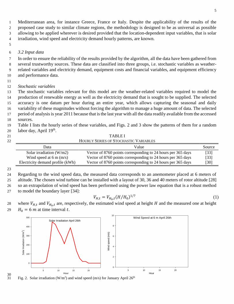
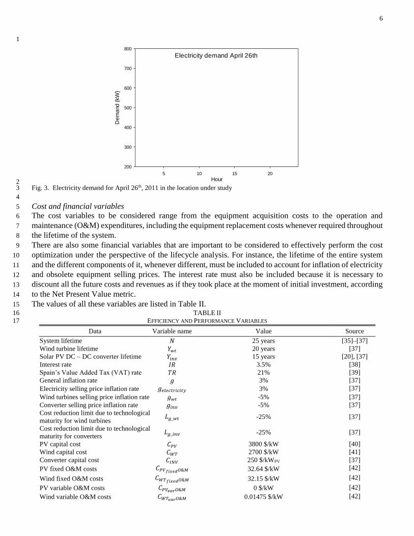
Table I lists the hourly series of these variables, and Figs. 2 and 3 show the patterns of them for a random 19

labor day, April 19th. 20

TABLE I 21

HOURLY SERIES OF STOCHASTIC VARIABLES 22

Data Value Source

Solar irradiation (W/m2) Vector of 8760 points corresponding to 24 hours per 365 days [33]

Wind speed at 6 m (m/s) Vector of 8760 points corresponding to 24 hours per 365 days [33]

Electricity demand profile (kWh) Vector of 8760 points corresponding to 24 hours per 365 days [30]

23

Regarding to the wind speed data, the measured data corresponds to an anemometer placed at 6 meters of 24

altitude. The chosen wind turbine can be installed with a layout of 30, 36 and 40 meters of rotor altitude [28] 25

so an extrapolation of wind speed has been performed using the power law equation that is a robust method 26

to model the boundary layer [34]: 27

𝑉𝐻,𝑡 = 𝑉𝐻0,𝑡(𝐻 𝐻0⁄ )1/7 (1)

where 𝑉𝐻,𝑡 and 𝑉𝐻0,𝑡 are, respectively, the estimated wind speed at height 𝐻 and the measured one at height 28

𝐻0 = 6 𝑚 at time interval 𝑡. 29

Solar Irradiation April 26th

Hour

5 10 15 20

Sola

r Ir

radia

tion (

W/m

2)

0

100

200

300

400

500 Wind Speed at 6 m April 26th

Hour

5 10 15 20

Win

d s

pe

ed

(m

/s)

0

2

4

6

8

10

30 Fig. 2. Solar irradiation (W/m2) and wind speed (m/s) for January April 26th 31

6

1

Electricity demand April 26th

Hour5 10 15 20

De

ma

nd

(kW

)

200

300

400

500

600

700

800

2 Fig. 3. Electricity demand for April 26th, 2011 in the location under study 3

4

Cost and financial variables 5

The cost variables to be considered range from the equipment acquisition costs to the operation and 6

maintenance (O&M) expenditures, including the equipment replacement costs whenever required throughout 7

the lifetime of the system. 8

There are also some financial variables that are important to be considered to effectively perform the cost 9

optimization under the perspective of the lifecycle analysis. For instance, the lifetime of the entire system 10

and the different components of it, whenever different, must be included to account for inflation of electricity 11

and obsolete equipment selling prices. The interest rate must also be included because it is necessary to 12

discount all the future costs and revenues as if they took place at the moment of initial investment, according 13

to the Net Present Value metric. 14

The values of all these variables are listed in Table II. 15

TABLE II 16

EFFICIENCY AND PERFORMANCE VARIABLES 17

Data Variable name Value Source

System lifetime 𝑁 25 years [35]–[37]

Wind turbine lifetime 𝑌𝑤𝑡 20 years [37]

Solar PV DC – DC converter lifetime 𝑌𝑖𝑛𝑣 15 years [20], [37]

Interest rate 𝐼𝑅 3.5% [38]

Spain’s Value Added Tax (VAT) rate 𝑇𝑅 21% [39]

General inflation rate 𝑔 3% [37]

Electricity selling price inflation rate 𝑔𝑒𝑙𝑒𝑐𝑡𝑟𝑖𝑐𝑖𝑡𝑦 3% [37]

Wind turbines selling price inflation rate 𝑔𝑤𝑡 -5% [37]

Converter selling price inflation rate 𝑔𝑖𝑛𝑣 -5% [37]

Cost reduction limit due to technological

maturity for wind turbines 𝐿𝑔_𝑤𝑡 -25% [37]

Cost reduction limit due to technological

maturity for converters 𝐿𝑔_𝑖𝑛𝑣 -25% [37]

PV capital cost 𝐶𝑃𝑉 3800 $/kW [40]

Wind capital cost 𝐶𝑊𝑇 2700 $/kW [41]

Converter capital cost 𝐶𝐼𝑁𝑉 250 $/kWPV [37]

PV fixed O&M costs 𝐶𝑃𝑉𝑓𝑖𝑥𝑒𝑑𝑂&𝑀 32.64 $/kW [42]

Wind fixed O&M costs 𝐶𝑊𝑇𝑓𝑖𝑥𝑒𝑑𝑂&𝑀 32.15 $/kW [42]

PV variable O&M costs 𝐶𝑃𝑉𝑣𝑎𝑟𝑂&𝑀 0 $/kW [42]

Wind variable O&M costs 𝐶𝑊𝑇𝑣𝑎𝑟𝑂&𝑀 0.01475 $/kW [42]

7

Electricity market price 𝐶𝑝𝑜𝑜𝑙 Vector of 8760 points; 24 hours per 365 days [43]

Electricity retail price 𝐶𝑒𝑙𝑒𝑐𝑡𝑟

Peak – 0.101406 €/kWh

Flat – 0.078289 €/kWh

Off-peak – 0.052683 €/kWh

[44]

Time periods

Peak: 17-23 winter/10-16 summer

Flat: 8-17, 23-24 winter /8-10,16-24 summer

Off-peak: 0-8 winter time / summer time

[45]

1

According to [40], PV system costs decrease exponentially as the size of installation increases, reaching an 2

average value of $3.8 per Watt for utility-scale installations that are those relevant for the scale of the 3

proposed case study. The values provided account for the cost of all the components of an installed system: 4

PV modules, converter, installation materials, labor costs, supply chain and even land acquisition and taxes, 5

commissioning and permitting costs. For residential or commercial scale equipment this value should be 6

changed to take into account the higher costs of the technology. 7

Regarding the wind power systems price, the data given in [41] also show an exponential decrease in price 8

with increasing project size. In this case, the entire cost of the system is also provided. 9

Furthermore, the electricity retail prices [44] have been introduced only taking into account the price of the 10

energy consumed, i.e. the cost of the kWh, and considering the different prices at different time 11

discrimination periods that the electrical bill has. The fixed costs derived from the contract like the cost of 12

the power contracted, are not introduced as the system is designed as grid-connected so they will be paid 13

regardless of the consumption that is what is expected to be reduced. For the market price of electricity, the 14

data of a whole year has been retrieved from the Iberian market operator OMIE [43], which provides the 15

clearing price in the pool of electricity with hourly accuracy that is the time period at which the auctions take 16

place. With these two datasets, it is possible to account for the benefits of selling electricity and costs of 17

purchasing it according to the positive production (surplus) or negative production (lack) of electricity at 18

each hour of the day. 19

These prices are considered to suffer an annual inflation of 3%, a conservative value according to last years’ 20

price change that doubled that value [46]. 21

22

Efficiency and performance variables 23

This set of data includes all the variables required to implement the performance calculation into the model. 24

That includes all the efficiencies of a solar PV installation and a wind turbine installation. For solar PV power, 25

these data include the module efficiency itself but also the wiring, converter and de-rating efficiencies among 26

others [40]; whereas for wind power that is acquired in the form of the characteristic curve of the wind turbine 27

provided by the manufacturer that includes all the efficiencies of the entire wind turbine [41]. 28

Table III shows the values used in the algorithm for all the variables that take a fixed value. 29

TABLE III 30

EFFICIENCY AND PERFORMANCE VARIABLES 31

Data Value Source

Module reference efficiency 15.0% [27]

Model nameplate de-rate 95.0% [47]

Converter efficiency 92.0% [47]

Module mismatch factor 98.0% [47]

Connections efficiency 99.5% [47]

DC wiring losses factor 98.0% [47]

AC wiring losses factor 99.0% [47]

Soiling de-rate factor 95.0% [47]

System availability O&M 98.0% [47]

8

1

In addition to such information, it is also important to introduce the PV power warranted by the manufacturer 2

curve [27], which diminishes over time as a result of aging (see Fig. 4) and the wind power characteristic 3

curve [28] (see Fig. 5) that shows the output of the wind turbine, including the wiring, generator, transformer 4

and power and control cabinet efficiencies. 5

The warranted power refers to the module reference efficiency, so the manufacturer warrants 97% of the 6

reference efficiency for the first two years and then the warranted power experiences a linear decline until 7

reaching 80% of the reference efficiency by the 30th year of module usage. 8

AM-5S Warranted Power

Year

0 5 10 15 20 25 30 35

Wa

rra

nte

d e

ffic

iency

ove

r re

fere

nce

va

lue

(%

)

78

80

82

84

86

88

90

92

94

96

98

100

9 Fig. 4. Warranted power (%) over lifetime of AS-5M PV module 10

11

SUT200 characteristic curve

Wind speed (m/s)

0 5 10 15 20 25 30

Po

we

r o

utp

ut (k

W)

0

50

100

150

200

250

12 Fig. 5. SUT200 characteristic curve, representing output power (kW) over wind speed (m/s) 13

14

15

3.3 Algorithm description 16

For HRESs optimization, as a result of the inherently non-linear variables found in this kind of problems 17

involving stochastic variables such as weather patterns [48] or electricity demand patterns, the most preferred 18

methodologies are GAs and particle swarm optimization (PSO) algorithms [19], both heuristic approaches. 19

Among the advantages of iterative algorithms highlight their low computational requirements that allow them 20

to obtain the desired solutions without requiring huge amounts of computational resources [49]. In particular, 21

GAs have been identified and used as one of the best alternatives for those cases where non-linear systems 22

are involved as HRES cost optimization problems are [50] even in cases with only few variables involved 23

because this method is very good attaining optimal solutions with non-linear relationships between variables 24

[9]. 25

The parameters that are usually analyzed for HRES optimization include not only the cost, which is the topic 26

at hand, but also the lifetime environmental impact of the system, the reliability of supply or a combination 27

9

of two or more of these parameters [35], [49]–[51], obtaining in such multi-objective case a set of possible 1

solutions called Pareto front. 2

The software used to run the optimization procedure is MATLAB R2013b, in which GAs are already 3

implemented in the “Optimization Toolbox”. 4

5

Variables 6

The variables chosen to represent the different potential alternative systems are the area covered by PV 7

modules 𝑝𝑣𝐴𝑟𝑒𝑎, which is proportional to the number of PV modules 𝑝𝑣𝑁𝑢𝑚𝑏𝑒𝑟, and the number of wind 8

turbines 𝑤𝑡𝑁𝑢𝑚𝑏𝑒𝑟. With these variables, the GA will treat the objective function as dependent of the system 9

sizing and will provide as outputs the minimum Net Present Value and the values of both variables that lead 10

to an optimal HRES sizing with a minimum 𝑁𝑃𝑉. 11

Wind turbine number variable is treated as an integer by the optimization algorithm. Conversely, the PV area 12

allows using decimal values thus reducing the computational requirements to run the GA. That is why the 13

area is selected as the variable rather than the number of PV modules. 14

15

Objective (fitness) function 16

The parameter that is sought to optimize in the present work is the cost of the system. Considering that 17

lifecycle perspective is currently gaining importance in HRES’ optimization methodologies [20], the 18

lifecycle cost has been chosen as the metric to optimize. To do so, the chosen objective function is the Net 19

Present Value (NPV) cost metric that is calculated by adding the discounted present values of all lifetime 20

incomes and subtracting the discounted present costs along lifetime of the system, i.e. considering the 21

expenses and revenues 25 years ahead. Therefore, this cost metric is accounting for the future cash-flows’ 22

present value by converting them to the value of money at the time of investment after applying inflation and 23

discount rate to all of them. Hence, the system lifetime costs can be analyzed discounting external effects 24

like the financial volatility or oscillations inherent to the free market economy that affect the value of money. 25

To appropriately compute all the costs throughout the entire lifetime of the system, the initial investment, 26

operation and maintenance, equipment replacement and electricity purchase costs have been taken into 27

account, similarly as done in [20]. On the other hand, the benefits from selling the electricity to the grid and 28

the profit from equipment sale at the end of the lifetime have been considered on the benefits side: 29

𝑁𝑃𝑉 = 𝐶𝑖𝑛𝑣𝑒𝑠𝑡𝑚𝑒𝑛𝑡 + 𝑁𝑃𝑉𝑂&𝑀 + 𝑁𝑃𝑉𝑟𝑒𝑝𝑙 − 𝑁𝑃𝑉𝑒𝑙𝑒𝑐𝑡𝑟𝑖𝑐𝑖𝑡𝑦 − 𝑁𝑃𝑉𝑒𝑛𝑑𝐿𝑖𝑓𝑒 = 𝑓(𝑝𝑣𝐴𝑟𝑒𝑎, 𝑤𝑡𝑁𝑢𝑚𝑏𝑒𝑟) (2)

(2) being the fitness function. In the following paragraphs, the five terms in (2) are detailed. 30

The initial investment cost refers to the initial expense required for equipment purchase. It has been 31

implemented as a function of the number of modules and the number of wind turbines installed: 32

𝐶𝑖𝑛𝑣𝑒𝑠𝑡𝑚𝑒𝑛𝑡 = 𝐶𝑃𝑉 · 𝑝𝑣𝑁𝑢𝑚𝑏𝑒𝑟 · 𝑃𝑚𝑜𝑑𝑢𝑙𝑒 + 𝐶𝑊𝑇 · 𝑤𝑡𝑁𝑢𝑚𝑏𝑒𝑟 · 𝑃𝑡𝑢𝑟𝑏𝑖𝑛𝑒 (3)

where 𝐶𝑃𝑉 is the capital cost of PV panels in $/kW, 𝑃𝑚𝑜𝑑𝑢𝑙𝑒 is the nominal power of each module; 𝐶𝑊𝑇 is 33

the capital cost of wind turbines in $/kW and 𝑃𝑡𝑢𝑟𝑏𝑖𝑛𝑒 is the wind turbine nominal power. As the input variable 34

is 𝑝𝑣𝐴𝑟𝑒𝑎, the number of PV modules is expressed as follows: 35

𝑝𝑣𝑁𝑢𝑚𝑏𝑒𝑟 = 𝑝𝑣𝐴𝑟𝑒𝑎/𝑝𝑎𝑛𝑒𝑙𝐴𝑟𝑒𝑎 36

where 𝑝𝑣𝐴𝑟𝑒𝑎 is the independent variable and 𝑝𝑎𝑛𝑒𝑙𝐴𝑟𝑒𝑎 is the area covered by a single PV module, in the 37

case study 1.277 m2. 38

The discounted operation and maintenance costs are calculated considering the annual inflation rate [37]: 39

𝑁𝑃𝑉𝑂&𝑀 = ∑ 𝐶𝑂&𝑀_𝑘

𝑁

𝑖=1

(1 + 𝑔)𝑖

(1 + 𝐼𝑅)𝑖 (4)

where 𝐶𝑂&𝑀_𝑘 refers to the cost of operation and maintenance of component 𝑘, 𝑔 is the general inflation rate, 40

𝐼𝑅 is the interest rate and 𝑁 is the system lifetime. 41

The discounted present costs of equipment replacement are also calculated considering the annual inflation 42

10

rate [37]: 1

𝑁𝑃𝑉𝑟𝑒𝑝𝑙_𝑘 = ∑ 𝐶𝑘

(1 + 𝑔𝑘)𝑖·𝑁𝑘

(1 + 𝐼𝑅)𝑖·𝑁𝑘

𝑁_𝑓𝑖𝑟𝑠𝑡𝑟𝑒𝑝𝑙_𝑘

𝑖=1

+ ∑ 𝐶𝑘

(1 + 𝑔𝑘)𝑌𝑘(1 + 𝑔)𝑖·𝑁𝑘−𝑌𝑘

(1 + 𝐼𝑅)𝑖·𝑁𝑘

𝑁_𝑟𝑒𝑝𝑙_𝑘

𝑖=𝑁𝑓𝑖𝑟𝑠𝑡𝑟𝑒𝑝𝑙+1

(5)

where 𝐶𝑘 is the acquisition cost of component 𝑘, 𝑔𝑘 is the expected inflation rate of the acquisition cost of 2

component 𝑘 and 𝑌𝑘 is the lifetime of such component. 𝑁𝑟𝑒𝑝𝑙𝑘 and 𝑁𝑓𝑖𝑟𝑠𝑡𝑟𝑒𝑝𝑙_𝑘 are the total number of 3

replacements during system lifetime and during the years that the price of the component is changing at 𝑔𝑘 4

inflation rate, respectively, and are calculated as follows [37]: 5

𝑁𝑟𝑒𝑝𝑙𝑘= 𝑖𝑛𝑡 [

𝑁

𝑌𝑘] (6)

𝑁𝑓𝑖𝑟𝑠𝑡𝑟𝑒𝑝𝑙_𝑘 = 𝑖𝑛𝑡 [𝑌𝑔_𝑘

𝑌𝑘] (7)

where 𝑌𝑔_𝑘 is the number of years required for technology 𝑘 to reach the technological maturity with a cost 6

reduction of 𝐿𝑔_𝑘 [37]: 7

𝑌𝑔_𝑘 =log(1 + 𝐿𝑔_𝑘)

log(1 + 𝑔𝑘) (8)

The PV – wind hybrid system that is being studied is considered to have a lifetime of 25 years which is the 8

lifetime of the component that lasts more, the PV module. Therefore, the costs of equipment replacement 9

only account for wind turbine and solar PV converter replacement, as the wind turbine has a lifetime of 20 10

years and solar PV converter has a lifetime of 15 years (see Table II). 11

The cost of electricity purchase and the benefits derived from electricity sale are computed together in the 12

algorithm. To effectively perform that, the hourly net power production is calculated by adding up the PV 13

power production (𝑁𝑃𝑃) and the wind power production and subtracting the electricity demand for each 14

hour: 15

𝑁𝑃𝑃 = 𝑃𝑃𝑉 + 𝑃𝑊𝑇 − 𝑑𝑒𝑚𝑎𝑛𝑑 (9)

where 𝑃𝑃𝑉 and 𝑃𝑊𝑇 are the PV and wind power produced at each hour of the 365 days of a year and 𝑑𝑒𝑚𝑎𝑛𝑑 16

is the electricity demand of the location under study. This point-to-point comparison of production and 17

demand allows implementing the annual net balance design condition as a forced zero sum of all the 8760 18

points. It also allows calculating the exact benefit or cost of selling or purchasing electricity according to the 19

hourly market and retail prices. 20

If the sign of (9) is positive, more power is produced than demanded so the electricity is sold at the market 21

price. Conversely, if the sign of the sum is negative, the system is producing less power than demanded so 22

the lack has to be purchased at the electricity retail price. This entire process is introduced in the algorithm 23

considering the electricity selling price inflation 𝑔𝑒𝑙𝑒𝑐𝑡𝑟𝑖𝑐𝑖𝑡𝑦 [37]. Therefore, for negative net power 24

production, the net present cost of electricity purchase is: 25

𝑁𝑃𝑉𝑒𝑙𝑒𝑐𝑡𝑟𝑖𝑐𝑖𝑡𝑦 = ∑ ∑ 𝐶𝑒𝑙𝑒𝑐𝑡𝑟_𝑗 · 𝑁𝑃𝑃𝑗 ·(1 + 𝑔𝑒𝑙𝑒𝑐𝑡𝑟𝑖𝑐𝑖𝑡𝑦)

𝑖

(1 + 𝐼𝑅)𝑖

8760

𝑗=1

𝑁

𝑖=1

(10)

And for positive net power production, the discounted present incomes from the selling of electricity are: 26

𝑁𝑃𝑉𝑒𝑙𝑒𝑐𝑡𝑟𝑖𝑐𝑖𝑡𝑦 = ∑ ∑ 𝐶𝑝𝑜𝑜𝑙_𝑗 · 𝑁𝑃𝑃𝑗 ·(1 + 𝑔𝑒𝑙𝑒𝑐𝑡𝑟𝑖𝑐𝑖𝑡𝑦)

𝑖

(1 + 𝐼𝑅)𝑖

8760

𝑗=1

𝑁

𝑖=1

(11)

It should be pointed out that in the first case, 𝑁𝑃𝑃 < 0 or lack of electricity, the 𝑁𝑃𝑉𝑒𝑙𝑒𝑐𝑡𝑟𝑖𝑐𝑖𝑡𝑦 will take 27

negative values whereas in the second case, 𝑁𝑃𝑃 > 0 or surplus of electricity, the 𝑁𝑃𝑉𝑒𝑙𝑒𝑐𝑡𝑟𝑖𝑐𝑖𝑡𝑦 will take 28

11

positive values. As a result, this term of 𝑁𝑃𝑉𝑒𝑙𝑒𝑐𝑡𝑟𝑖𝑐𝑖𝑡𝑦 is computed in the benefits side as previously 1

mentioned. 2

The last term of the 𝑁𝑃𝑉 calculation is the discounted present value of incomes from the sale of equipment 3

at the end of system lifetime [37], and is also computed in the benefits side of the NPV calculation. 4

𝑁𝑃𝑉𝑒𝑛𝑑𝐿𝑖𝑓𝑒_𝑘 = 𝐶𝑘 [1 −𝑁𝑟𝑒𝑝𝑙_𝑘𝑌𝑘

𝑁] (

(1 + 𝑔𝑘)𝑌𝑔_𝑘(1 + 𝑔)𝑁−𝑌𝑔_𝑘

(1 + 𝐼𝑅)𝑁) (12)

The entire methodology of the proposed grid-connected HRES power balance approach is detailed in Fig. 6. 5

Renewable Energy Sources (RES)

Solar Irradiation data

Wind speed data

Load profile (demand)

MATLAB R2013 RES model

simulation

PV power production (PPV)

Wind power production (PWT)

Cost parameters

Technology cost

O&M cost

Electricity market and retail price

RES models and parameters

Solar PV model (global efficiency)

Wind turbine model (characterisc

curve)

MATLAB R2013 optimization

Controlled elitist genetic

algorithm (see Fig. 7)

Other NPV terms

calculation

From eq. 3-5, 12

Point-to-point electricity production/consumption

balance

11 eq. from If

10 eq. from If

yelectricitWTPV

yelectricitWTPV

NPVdemandPP

NPVdemandPP

.

Optimal system

sizing

pvArea

wtNumber

Minimum NPV?

NO

YES

6 Fig. 6. Proposed HRES cost optimization approach 7

8

Optimization process 9

Once the objective function is properly defined and all the input variables introduced, the optimization 10

algorithm can be run. From all the available alternatives, the GA optimization methodology has been selected 11

for its easiness to tackle multiple solution problems using a random population of potential solutions and 12

evolutionary methods to narrow down the possibilities according to the fitness of each possible solution until 13

finding the optimum. The methodology starts with the generation of a random population with a size of: 14

𝑃𝑜𝑝𝑢𝑙𝑎𝑡𝑖𝑜𝑛𝑆𝑖𝑧𝑒 = max (min(10 · 𝑛𝑢𝑚𝑏𝑒𝑟𝑂𝑓𝑉𝑎𝑟𝑠, 100) , 40) (13)

From this population the best individuals are selected according to the fitness function that is sought to 15

optimize. The individuals are scaled by a “Rank” criterion meaning that the top individuals are selected; in 16

this case, 5% is selected: 17

𝐸𝑙𝑖𝑡𝑒𝐶𝑜𝑢𝑛𝑡 = 0.05 · max (min(10 · 𝑛𝑢𝑚𝑏𝑒𝑟𝑂𝑓𝑉𝑎𝑟𝑠, 100) , 40) (14)

Once they are selected, a new generation of “offspring” individuals is created crossover that is the creation 18

of a new individual or child from two existent individuals or parents, of existent specimens. The crossover 19

fraction is set to 80% and the method to “Scattered”. Mutation does not occur because this process is ignored 20

with one or more integer variables. Migration is another process that allows movement of individuals within 21

the space of solutions. In this case, 20% of individuals migrate in “forward” direction every 20 generations. 22

From the old set of individuals, the “least-fit” individuals are rejected and replaced by the new generation 23

and this process is repeated many times until the minimum value of the fitness function is found. The stopping 24

criterion is the condition of having an average change in the fitness function value below the function 25

tolerance, in this case 1 · 10−6 once the stall generation, in this case 50, is reached. 26

12

Input variables upper and lower bounds are used to introduce restrictions in the potential solutions, so the 1

lower bounds are 0 m2 of area covered by PV modules and 0 wind turbines, the case of no system installed. 2

The upper bounds set are the maximum allowable installed capacity of each renewable energy source. They 3

have been assumed to be higher enough to not introduce any limitation but they could be set to a certain value 4

if there were limitations in terms of maximum initial investment or available land useful to install the 5

equipment, for instance. 6

Fig. 7 schematizes the optimization process by means of GA and specifies the selected parameters: 7

Random generation of a population with a size

PopulationSize (Eq.13)

of 2-variables (pvArea, wtNumber) individuals

Net power production (NPP) calculation (Eq.9)

for all the individuals

Objective function evaluation

From Eq. 3-5, 10-12

Yes

No

Input Variables

Electricity demand and weather-related variables

Cost and financial variables

Efficiency and performance variables

Bounds and GA parameters

Tolerance error < ?

Crossover

Scattered, 80%

No

Selection of best-fit

individuals

Rank selection, Elite = 5%

Optimum HRES

sizing

Yes

?08760

1

8760

1

i

i

i

i demandNPP

Eq.(2) from ),( wtNumberpvAreafNPV

8 Fig. 7. Optimization model and parameters 9

10

4. RESULTS 11

With aim to contextualize the values obtained, all the simulated cases are compared with the no-HRES case, 12

13

i.e. the case of a system with no solar nor wind renewable sources. This is a reduction of the general case 1

used to estimate the cost of supplying the demand according to the actual situation in which the electricity is 2

purchased from the local utility at the market retail price. 3

4

4.1 No-HRES scenario 5

The no-HRES case is obtained by running the algorithm with zero solar PV power and zero wind power 6

production. 7

The total electricity demand in one year, obtained from the data in [30], equals 4657.97 MWh. The cost of 8

supplying this demand during the 25 years that a HRES would last, and considering the actual demand at 9

each hour is purchased at the price established in the tariff with hourly discrimination is: 10

𝑛𝑜 − 𝐻𝑅𝐸𝑆 𝑁𝑃𝑉 = $2.3446 · 107 = $23.446M 11

That would be the total cost of supplying the present demand considering that electricity price suffers an 12

annual inflation of 3% (see Table II). 13

14

4.2 HRES base case scenario 15

The base-case is the case simulated using all the variables as previously defined in Tables I, II and III and 16

Figs. 3 and 4. The wind data used have been extrapolated to 35m of rotor height, found at the middle between 17

30 and 40 m, the minimum and maximum values provided by the manufacturer [28]. The optimization 18

procedure provides the following result: 19

𝑏𝑎𝑠𝑒 − 𝑐𝑎𝑠𝑒 𝑁𝑃𝑉 = $1.5353 · 107 = $15.353M 20

This result is reached with a system with 621.61m2 of PV installation and 18 wind turbines, equivalent to 21

102.22 kW of PV power and 3.6 MW of wind power, a HRES that would require an initial investment of 22

$1.0108 · 107 = $10.108M. 23

For comparison purposes, the evolution of NPV of No-HRES and base case scenarios during the system 24

lifetime are shown in Fig. 7. 25

Annual NPV Comparison

Year

0 5 10 15 20 25

NP

V (

M$

)

0

5

10

15

20

25

No-HRES NPV

HRES base case NPV

26 Fig. 7. Comparison of NPV evolution throughout 25 years of system lifetime for No-HRES and HRES base case scenarios 27

28

4.3 Sensitivity analysis 29

The sensitivity analysis is performed introducing percent variations in the most relevant parameters of the 30

system to observer how these variations vary the output of the system. 31

The variables chosen to be studied in this sensitivity analysis are: PV technology capital cost, wind 32

technology capital cost, electricity price, general inflation rate, module and wind turbine reference 33

14

efficiencies and interest rate. The change introduced in the values of these variables induces variations in the 1

result of different magnitude. The results are shown in Table IV. 2

TABLE IV 3

SENSITIVITY ANALYSIS 4

Variable Variation NPV change

PV capital cost +10% +0.261%

Wind capital cost +10% +9.381%

Electricity price +10% +0.000%

General inflation rate (g) +10% +1.238%

Interest rate +10% -2.002%

Module reference efficiency +10% -0.261%

Wind turbine reference efficiency +10% -8.599%

5

5 DISCUSSION 6

The Net Present Value of the HRES base case is $15.535, 65.26% of the no-HRES NPV. However, the 7

system requires an initial investment of $10.108M. This significant upfront investment required is the main 8

hurdle to be overcome by renewable energy technologies. However, when the evolution of NPV during 9

system lifetime for both base case and no-HRES scenarios are compared, it emerges that the installation of a 10

HRES implies higher accumulated costs during first years, a tendency that is inverted approximately after 11

two thirds of system life time. In particular, with the proposed case study the system would imply less 12

accumulated costs from 18th year onwards (see Fig. 7). Therefore, even though the required investment is a 13

significant amount that is never paid off, the system proves to be worthwhile once the current situation costs 14

are taken into consideration. Besides, the NPV evolution throughout system lifetime also shows that policies 15

that would improve RES profitability could act either on the slope of the curve or in the huge jump that is 16

observed in the first year. To influence on the former, one could subsidize the renewable electricity sale, for 17

instance introducing a feed-in tariff that would increase the electricity selling price and thus invert the slope 18

of the curve; whereas to influence on the latter, one should subsidize the installation of renewable energy 19

systems. The first solution has been adopted in countries like Germany, Spain or Australia, whereas the 20

second is the alternative proposed in some US States like California. 21

From the sensitivity analysis results, it is shown that the most significant parameter analyzed is the wind 22

capital cost. That is because the optimal sizing found by the algorithm consists on a 3.6 MW wind installation 23

for the 0.1 MW of solar PV power, so changes in the cost of the component that represents more than 95% 24

of the total installation are expected to affect more the final NPV than changes in the cost of the component 25

that represents less than 5% of installation size. 26

Furthermore, it is shown that the electricity price does not significantly affect the result, so the installation is 27

expected to have the reported profitability regardless of the inflation of electricity price. This effect is caused 28

by the low impact of electricity purchasing prices on the system as it is based on the reduction of electricity 29

consumption from the grid. Conversely, the inflation in the retail electricity prices would affect the break-30

even point as the no-HRES scenario would see its costs surge, making the installation of the HRES system 31

more worthwhile compared with the business-as-usual alternative. 32

The last analyzed variable is the interest rate. Increases in this variable result in decreases in the NPV as they 33

mean more money value discount in future years. That is why in the NPV definition itself the interest rate is 34

dividing several terms (see (4), (5), (10)-(12)). This behavior shows the effect of time value of money, which 35

means that a certain amount of money is worth more at present time that in the future, and that this discounted 36

present value is lower as higher is the discount rate. The chosen value in the base case of 3.5% is a reasonable 37

approach considering the current interest rates for loans to non-financial corporations in Spain that averaged 38

3.5% in the last 10 years [38]. 39

15

It is also worth mentioning that the system sizing does not suffer changes with the first five cases, PV and 1

wind capital cost, electricity price, general inflation rate and interest rate; but with the other two cases, PV 2

module and wind turbine efficiency improvements, the system sizing is changed. On the one hand, with 10% 3

improvement in the PV module reference efficiency, the new HRES consists of 18 wind turbines and 4

565.13m2 of PV installation, being the total installed capacity the same as in the base case scenario but with 5

10% less land usage for the PV installation. On the other hand, with 10% improvement in the wind turbine 6

reference efficiency, the new HRES consists of 17 wind turbines and PV installation reduced to a marginal 7

size, the total installed capacity remaining again unchanged at roughly 3.7MW but with different share of 8

each RE technology. 9

10

6 CONCLUSIONS 11

An optimization algorithm that calculates the optimum sizing for a grid-connected HRES according to a 12

given electricity demand has been developed and tested through a case study. The HRES combines solar PV 13

and wind power technologies at the most appropriate scales to supply the existent demand with a minimum 14

life cycle cost that is measured using the Net Present Value, an economic metric that discounts the future 15

costs and revenues at the time of investment. The designed optimization algorithm performs an analysis with 16

one hour accuracy in order to capture the daily and seasonal patterns of both weather-dependent renewable 17

energies and electricity demand. Moreover, it performs a meticulous calculation of the renewable electricity 18

generation patterns and thus the profits and revenues derived from it, not only because of the different amount 19

of energy produced at each hour but also because of the consideration of the different market and retail prices 20

at each hour of the day. 21

A sensitivity analysis has been performed through the simulation of slight variations of a base case that served 22

to understand the behavior of the results given by the algorithm in front of changes in the most important 23

input variables. Such analysis also includes a comparison with the no-HRES scenario that helps 24

understanding how significant are the cost savings compared with the present situation costs. 25

Another aspect to highlight is that the algorithm responds well to positive and negative changes in the 26

analyzed variables. For instance, the NPV obtained from the algorithm increases when cost variables 27

increase, whereas decreases when efficiency of RE technologies improves. Again, wind turbine efficiency 28

improvements have greater impacts on the result than PV panel efficiency improvements due to the greater 29

importance of wind installation in the case under study. 30

The results, therefore, show that in the location under study wind power is the renewable resource with greater 31

impact but that it is well complemented by solar resource. Such HRES also proves its appropriateness to 32

replace the present scenario in which electricity consumption is only supplied by the electrical grid, with 33

potential savings amounting up to 40% of present cost structure throughout the next 25 years. 34

35

REFERENCES 36

[1] B. Buragohain, P. Mahanta, and V. S. Moholkar, “Biomass gasification for decentralized power 37

generation: The Indian perspective,” Renew. Sustain. Energy Rev., vol. 14, no. 1, pp. 73–92, 2010. 38

[2] B. Zhao, X. Zhang, P. Li, K. Wang, M. Xue, and C. Wang, “Optimal sizing, operating strategy and 39

operational experience of a stand-alone microgrid on Dongfushan Island,” Appl. Energy, vol. 113, 40

pp. 1656–1666, Jan. 2014. 41

16

[3] L. Montuori, M. Alcázar-Ortega, C. Álvarez-Bel, and A. Domijan, “Integration of renewable energy 1

in microgrids coordinated with demand response resources: Economic evaluation of a biomass 2

gasification plant by Homer Simulator,” Appl. Energy, vol. 132, pp. 15–22, Nov. 2014. 3

[4] V. Kuhn, J. Klemeš, and I. Bulatov, “MicroCHP: Overview of selected technologies, products and 4

field test results,” Appl. Therm. Eng., vol. 28, no. 16, pp. 2039–2048, 2008. 5

[5] D. Silva Herran and T. Nakata, “Design of decentralized energy systems for rural electrification in 6

developing countries considering regional disparity,” Appl. Energy, vol. 91, no. 1, pp. 130–145, Mar. 7

2012. 8

[6] M. Ranaboldo, B. D. Lega, D. V. Ferrenbach, L. Ferrer-Martí, R. P. Moreno, and A. García-Villoria, 9

“Renewable energy projects to electrify rural communities in Cape Verde,” Appl. Energy, vol. 118, 10

pp. 280–291, Apr. 2014. 11

[7] T. Ma, H. Yang, and L. Lu, “A feasibility study of a stand-alone hybrid solar–wind–battery system 12

for a remote island,” Appl. Energy, vol. 121, pp. 149–158, May 2014. 13

[8] M. K. Deshmukh and S. S. Deshmukh, “Modeling of hybrid renewable energy systems,” Renew. 14

Sustain. Energy Rev., vol. 12, no. 1, pp. 235–249, 2008. 15

[9] T. Ma, H. Yang, L. Lu, and J. Peng, “Pumped storage-based standalone photovoltaic power 16

generation system: Modeling and techno-economic optimization,” Appl. Energy, Jun. 2014. 17

[10] F. Calise, A. Cipollina, M. Dentice d’Accadia, and A. Piacentino, “A novel renewable 18

polygeneration system for a small Mediterranean volcanic island for the combined production of 19

energy and water: Dynamic simulation and economic assessment,” Appl. Energy, vol. 135, pp. 675–20

693, Dec. 2014. 21

[11] H.-C. Chen, “Optimum capacity determination of stand-alone hybrid generation system considering 22

cost and reliability,” Appl. Energy, vol. 103, pp. 155–164, Mar. 2013. 23

[12] A. T. D. Perera, R. A. Attalage, K. K. C. K. Perera, and V. P. C. Dassanayake, “A hybrid tool to 24

combine multi-objective optimization and multi-criterion decision making in designing standalone 25

hybrid energy systems,” Appl. Energy, vol. 107, pp. 412–425, Jul. 2013. 26

[13] A. T. D. Perera, R. A. Attalage, K. K. C. K. Perera, and V. P. C. Dassanayake, “Designing 27

standalone hybrid energy systems minimizing initial investment, life cycle cost and pollutant 28

emission,” Energy, vol. 54, pp. 220–230, Jun. 2013. 29

[14] B. Bhandari, K.-T. Lee, C. S. Lee, C.-K. Song, R. K. Maskey, and S.-H. Ahn, “A novel off-grid 30

hybrid power system comprised of solar photovoltaic, wind, and hydro energy sources,” Appl. 31

Energy, vol. 133, pp. 236–242, Nov. 2014. 32

[15] T. Ma, H. Yang, L. Lu, and J. Peng, “Optimal design of an autonomous solar–wind-pumped storage 33

power supply system,” Appl. Energy, Dec. 2014. 34

[16] G. Bekele and G. Tadesse, “Feasibility study of small Hydro/PV/Wind hybrid system for off-grid 35

rural electrification in Ethiopia,” Appl. Energy, vol. 97, no. 0, pp. 5–15, 2012. 36

17

[17] G. Bekele and B. Palm, “Feasibility study for a standalone solar–wind-based hybrid energy system 1

for application in Ethiopia,” Appl. Energy, vol. 87, no. 2, pp. 487–495, 2010. 2

[18] S. Rehman, M. Mahbub Alam, J. P. Meyer, and L. M. Al-Hadhrami, “Feasibility study of a wind–3

pv–diesel hybrid power system for a village,” Renew. Energy, vol. 38, no. 1, pp. 258–268, 2012. 4

[19] M. Fadaee and M. A. M. Radzi, “Multi-objective optimization of a stand-alone hybrid renewable 5

energy system by using evolutionary algorithms: A review,” Renew. Sustain. Energy Rev., vol. 16, 6

no. 5, pp. 3364–3369, 2012. 7

[20] D. Abbes, A. Martinez, and G. Champenois, “Life cycle cost, embodied energy and loss of power 8

supply probability for the optimal design of hybrid power systems,” Math. Comput. Simul., vol. 98, 9

pp. 46–62, Apr. 2014. 10

[21] Y. Hu and P. Solana, “Optimization of a hybrid diesel-wind generation plant with operational 11

options,” Renew. Energy, vol. 51, pp. 364–372, Mar. 2013. 12

[22] J. K. Kaldellis, K. A. Kavadias, and A. E. Filios, “A new computational algorithm for the calculation 13

of maximum wind energy penetration in autonomous electrical generation systems,” Appl. Energy, 14

vol. 86, no. 7–8, pp. 1011–1023, Jul. 2009. 15

[23] M. Alsayed, M. Cacciato, G. Scarcella, and G. Scelba, “Multicriteria Optimal Sizing of 16

Photovoltaic-Wind Turbine Grid Connected Systems,” IEEE Trans. Energy Convers., vol. 28, no. 2, 17

pp. 370–379, Jun. 2013. 18

[24] T. Ma, H. Yang, L. Lu, and J. Peng, “Technical feasibility study on a standalone hybrid solar-wind 19

system with pumped hydro storage for a remote island in Hong Kong,” Renew. Energy, vol. 69, pp. 20

7–15, Sep. 2014. 21

[25] M. Kapsali, J. S. Anagnostopoulos, and J. K. Kaldellis, “Wind powered pumped-hydro storage 22

systems for remote islands: A complete sensitivity analysis based on economic perspectives,” Appl. 23

Energy, vol. 99, pp. 430–444, Nov. 2012. 24

[26] G. Baquero, B. Esteban, J.-R. Riba, A. Rius, and R. Puig, “An evaluation of the life cycle cost of 25

rapeseed oil as a straight vegetable oil fuel to replace petroleum diesel in agriculture,” Biomass and 26

Bioenergy, vol. 35, no. 8, pp. 3687–3697, Aug. 2011. 27

[27] Amerisolar, “AmeriSolar AS-5M,” 2013. [Online]. Available: http://www.weamerisolar.com/. 28

[28] Generation Wind Ltd, “SUT200 wind turbine,” 2014. [Online]. Available: 29

http://www.generationwindturbines.com/en/our-turbines/product-range/sut-200. 30

[29] IDESCAT, “Santa Coloma de Queralt - The township in figures,” 2011. [Online]. Available: 31

http://www.idescat.cat/emex/?id=431397#h40000. 32

[30] Electra Caldense, “Hourly demand data.” Caldes de Montbui, Spain, 2011. 33

[31] IDAE, “Análisis del consumo energético del sector residencial en España INFORME FINAL,” 34

Madrid, Spain, 2011. 35

18

[32] Eurostat, “Electricity and Natural Gas price statistics,” 2014. [Online]. Available: 1

http://epp.eurostat.ec.europa.eu/statistics_explained/index.php/electricity_and_natural_gas_price_sta2

tistics. 3

[33] Meteorological Service of Catalonia (Meteocat), “Hourly data of UJ automatic weather station.” 4

Generalitat de Catalunya, Barcelona, Spain, 2012. 5

[34] S. Blumsack and K. Richardson, “Cost and emissions implications of coupling wind and solar 6

power,” Smart Grid Renew. Energy, vol. 3, no. 4, pp. 308–315, 2012. 7

[35] R. Dufo-López and J. L. Bernal-Agustín, “Design and control strategies of PV-Diesel systems using 8

genetic algorithms,” Sol. Energy, vol. 79, no. 1, pp. 33–46, 2005. 9

[36] J. Hernández-Moro and J. M. Martínez-Duart, “Analytical model for solar PV and CSP electricity 10

costs: Present LCOE values and their future evolution,” Renew. Sustain. Energy Rev., vol. 20, pp. 11

119–132, 2013. 12

[37] R. Dufo-López, J. L. Bernal-Agustín, and F. Mendoza, “Design and economical analysis of hybrid 13

PV–wind systems connected to the grid for the intermittent production of hydrogen,” Energy Policy, 14

vol. 37, no. 8, pp. 3082–3095, Aug. 2009. 15

[38] INE, “Spain: Economic and financial data,” 2014. [Online]. Available: 16

http://www.ine.es/dynt3/FMI/en/. 17

[39] Agencia Tributaria, “Impuesto Sobre el Valor Añadido,” 2014. [Online]. Available: 18

http://www.agenciatributaria.es/AEAT.internet/Inicio_es_ES/La_Agencia_Tributaria/Normativa/Nor19

mativa_tributaria_y_aduanera/Impuestos/Impuesto_sobre_el_valor_anadido__IVA_/Impuesto_sobre20

_el_valor_anadido__IVA_.shtml. 21

[40] A. Goodrich, T. James, and M. Woodhouse, “Residential, Commercial, and Utility-Scale 22

Photovoltaic (PV) System Prices in the United States: Current Drivers and Cost-Reduction 23

Opportunities,” Golden, CO, USA, 2012. 24

[41] R. Wiser and M. Bolinger, “2012 Wind technologies market report,” 2013. 25

[42] OpenEI, “Transparent cost database,” 2012. [Online]. Available: http://en.openei.org/apps/TCDB/. 26

[43] OMIE, “Resultados del mercado diario,” 2011. [Online]. Available: http://www.omie.es/inicio. 27

[44] Elèctrica de Santa Coloma, “High voltage price 3.0 fare.” 2014. 28

[45] Endesa, “High voltage time periods,” 2014. [Online]. Available: 29

https://www.endesaonline.com/ES/empresas/luz/tarifas_electricas_empresas_alta_tension/optima/ho30

ras/index.asp. 31

[46] OMIE, “Precio final anual de demanda nacional,” 2014. [Online]. Available: 32

http://www.omie.es/files/flash/ResultadosMercado.swf. 33

19

[47] Alliance for Sustainable Energy, “PV Watts calculator.” National Renewable Energy Laboratory 1

(NREL), Golden, CO, USA, 2013. 2

[48] R. Luna-Rubio, M. Trejo-Perea, D. Vargas-Vázquez, and G. J. Ríos-Moreno, “Optimal sizing of 3

renewable hybrids energy systems: A review of methodologies,” Sol. Energy, vol. 86, no. 4, pp. 4

1077–1088, 2012. 5

[49] J. L. Bernal-Agustín and R. Dufo-López, “Efficient design of hybrid renewable energy systems 6

using evolutionary algorithms,” Energy Convers. Manag., vol. 50, no. 3, pp. 479–489, 2009. 7

[50] E. Koutroulis, D. Kolokotsa, A. Potirakis, and K. Kalaitzakis, “Methodology for optimal sizing of 8

stand-alone photovoltaic/wind-generator systems using genetic algorithms,” Sol. Energy, vol. 80, no. 9

9, pp. 1072–1088, 2006. 10

[51] R. Baños, F. Manzano-Agugliaro, F. G. Montoya, C. Gil, A. Alcayde, and J. Gómez, “Optimization 11

methods applied to renewable and sustainable energy: A review,” Renew. Sustain. Energy Rev., vol. 12

15, no. 4, pp. 1753–1766, 2011. 13

14