optimal synthesis of heat exchanger networks involving...

1

Optimal Synthesis of Heat Exchanger Networks

Involving Isothermal Process Streams

José M. Ponce-Ortegaa,b, Arturo Jiménez-Gutiérreza*, and Ignacio E. Grossmannc

aDepartamento de Ingeniería Química, Instituto Tecnológico de Celaya, Celaya, Gto. 38010, México.

bFacultad de Química, Universidad Michoacana de San Nicolás de Hidalgo, Morelia, Mich. 58060, México.

cChemical Engineering Department, Carnegie Mellon University, Pittsburgh, PA 15213, USA.

Abstract

This paper proposes a new MINLP model for heat exchanger network synthesis that includes

streams with phase change. The model considers every possible combination of process streams that

may arise within a chemical process: streams with sensible heat, streams with latent heat, and streams

with both latent and sensible heat. As part of the optimization strategy, the superstructure is modeled

with logical conditions that are used for the proper placement of heat integration for streams with

change of phase. The proposed MINLP model provides the network structure that minimizes the total

yearly cost. Several examples are presented to illustrate the capabilities of the proposed model.

Keywords: Heat exchanger networks; Optimization; MINLP; Isothermal streams; Latent heat.

*Corresponding author. Telephone (+52-461) 611-7575. Fax: (+52-461) 611-7744. e-mail:

[email protected]

2

1. Introduction

Heat exchanger networks have been the subject of numerous investigations in the past decades

because of their impact in the energy recovery of industrial plants. Two major methodologies haven

been proposed for the synthesis of heat exchanger network problem, namely the sequential and the

simultaneous approach. One of the most-widely known sequential approaches is the pinch point design

method (Linnhoff and Hindmarsh, 1983), in which targets for the minimum utility requirement, the

minimum number of exchanger units and the minimum capital cost of the network are obtained

sequentially. Several heuristic rules are then used to synthesize a network that approaches these targets.

Other methodologies based on mathematical programming techniques to predict the minimum utility

requirements include the transportation problem formulation by Cerda et al. (1983) and the

transshipment problem approach by Papoulias and Grossmann (1983).

Works based on the simultaneous approach solve the problem without any decomposition, and

can explicitly handle the trade-offs between the capital and operational costs of the network. As part of

this approach, the work by Yee and Grossmann (1990) has provided a basic framework through the use

of a staged-superstructure that was formulated as a MINLP model with the objective of minimizing

simultaneously the utilities and capital costs of the network. Some extensions to such framework

include the works by Verheyen and Zhang (2006), Chen and Hung (2004) and Konukman et al. (2002)

that incorporated some flexibility aspects into the design of heat exchanger networks. The works by

Serna et al. (2004), Mizutani et al. (2003) and Frausto et al. (2003) have also extended the work of Yee

and Grossmann (1990) to incorporate detailed exchanger design models as well as pressure drop

equations. Sorsak and Kravanja (2004) and Ma et al. (2000) have formulated MINLP models for the

retrofit of heat exchanger networks. For a recent review on methodologies for the synthesis of heat

exchanger networks, see the paper by Furman and Sahinidis (2002).

Most of the methodologies proposed to solve the heat exchangers network problem have not

considered isothermal streams with phase change (i.e. streams that transfer their latent heat). Isothermal

streams arise for instance as part of separation processes and refrigeration sections. They also arise as an

3

approximation of multicomponent streams that undergo phase change in the coolers and reboilers in

distillation columns. Furthermore, streams with phase change include the subcooling and partial

condensation of outlet of reactor streams. Methodologies reported for the synthesis of heat exchanger

networks for isothermal streams, and more generally with phase change, have typically oversimplified

the problem, for instance by assuming 1 K drop or increase in the temperature of these streams. Hence,

no rigorous model has been reported to handle this kind of problem.

As part of an optimization model for simultaneous flowsheet optimization and heat integration,

Grossmann et al. (1988) modeled the pinch location strategy by Duran and Grossmann (1986) for non-

isothermal and isothermal streams using disjunctive programming. However, this method does not

synthesize network structures. Castier and Queiroz (2002) reported a methodology based on the pinch

point method to solve the energy targeting problem considering streams with phase changes. Liporace et

al. (2004) presented an alternative simplified procedure in which the streams with phase change are split

into sub-streams. The last two methodologies are sequential in nature, such that the trade-off between

capital and energy costs may not be properly achieved.

To provide some insight into the issue of streams with phase change, Figure 1 shows the

composites curves (Linnhoff and Flower, 1978) for a problem that includes both isothermal and non

isothermal streams. The horizontal segments represent the isothermal streams. The problem poses an

interesting modeling challenge for a proper mathematical programming formulation. For instance, one

could in principle decompose the streams that undergo a change of phase into substreams for the

superheated, saturated and subcooled parts. Aside from leaving open the question on how best to handle

the isothermal streams for the saturated section, this approach would lead to solutions with one

exchanger for each part of the heat content of the stream, which would most likely not provide the

optimal solution to the original problem.

We present in this paper a rigorous model for the synthesis of heat exchanger networks that

includes isothermal streams. The proposed model, which uses as a basis the MINLP model by Yee and

4

Grossmann (1990), is extended with appropriate constraints that allow the handling of isothermal

streams with only phase change and streams that also involve sensible heat effects.

Figure 1. Composite curves for a problem that includes isothermal and non isothermal streams

2. Outline of the proposed model

If one considers that process streams can exchange sensible and latent heats, three types of

situations can occur for heat transfer between any hot and any cold stream within a process. Figure 2

shows the temperature profiles for the three different types of hot and cold streams that will be

considered. The proposed model can handle any type of exchange between these streams. It is worth

mentioning that virtually all methods reported for the synthesis of heat exchanger networks have been

based on heat exchanges for only cases (a) and (d) in Figure 2.

5

a) Sensible heat

( )i i i iQ FCp TIN TOUT= −

b) Isothermal

condi iQ Fλ=

c) Sensible and latent heat

( )( )

suph cond condi i i i i

subc condi i i

Q FCp TIN T F

FCp T TOUT

λ= − +

+ −superheated

saturatedsubcooled

d) Sensible heat

( )j j j jQ FCp TOUT TIN= −

e) Isothermal

evapj jQ Fλ=

f) Sensible and latent heat

( )( )

suph evap evapj j j j j

subc evapj j j

Q FCp TOUT T F

FCp T TIN

λ= − +

+ −

superheated

saturatedsubcooled

Set Set Set

Set Set Set

TIN

TIN

TIN

TIN

TIN

TIN

TOUT

TOUT

TOUT

TOUT

TOUT

TOUT

Figure 2. Types of streams considered in the model

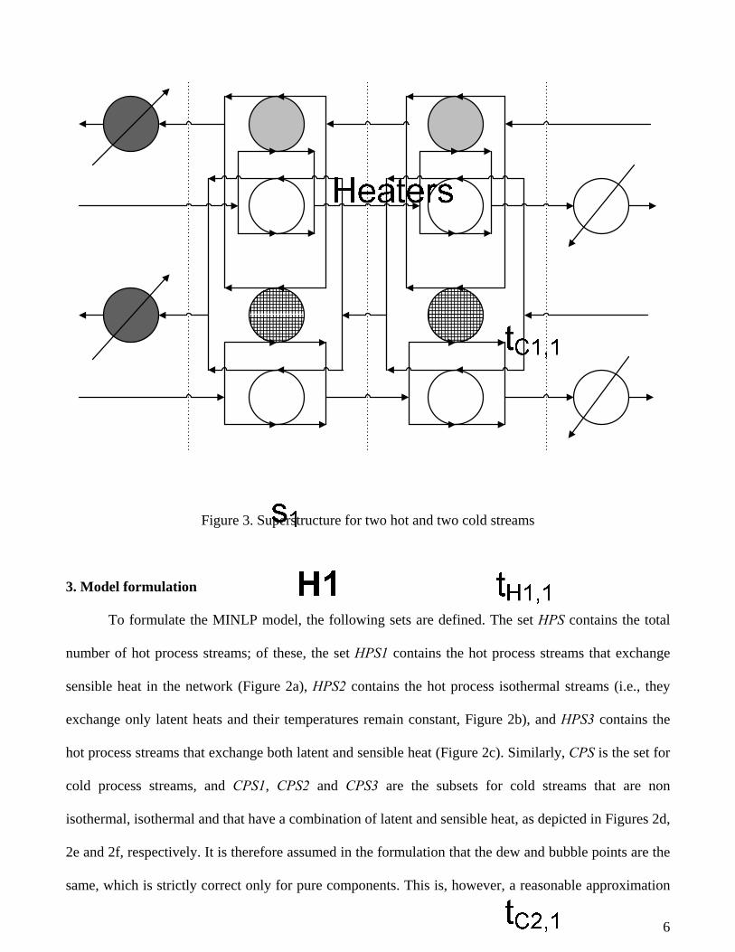
The proposed MINLP model that includes isothermal and non-isothermal streams is based on the

superstructure formulation by Yee and Grossman (1990). Figure 3 shows a superstructure involving two

hot and two cold process streams. The number of stages in the superstructure is commonly specified as

max{NH, NC}. In each stage of the superstructure, stream splitting is allowed to provide the possibility

of heat exchange between hot and cold streams. Within the formulation, isothermal mixing is assumed

with which it is only necessary to consider inlet and outlet temperatures at each stage of the

superstructure, and no variables for the flows are required. These intermediate temperatures in the

superstructure are treated as optimization variables, and the utility exchangers are placed in the extremes

of the superstructure.

6

Figure 3. Superstructure for two hot and two cold streams

3. Model formulation

To formulate the MINLP model, the following sets are defined. The set HPS contains the total

number of hot process streams; of these, the set HPS1 contains the hot process streams that exchange

sensible heat in the network (Figure 2a), HPS2 contains the hot process isothermal streams (i.e., they

exchange only latent heats and their temperatures remain constant, Figure 2b), and HPS3 contains the

hot process streams that exchange both latent and sensible heat (Figure 2c). Similarly, CPS is the set for

cold process streams, and CPS1, CPS2 and CPS3 are the subsets for cold streams that are non

isothermal, isothermal and that have a combination of latent and sensible heat, as depicted in Figures 2d,

2e and 2f, respectively. It is therefore assumed in the formulation that the dew and bubble points are the

same, which is strictly correct only for pure components. This is, however, a reasonable approximation

7

for many multicomponent mixtures, since very often the differences between dew and bubble points are

small. Also, a detailed model for the dependence of temperature with latent heat is not considered in this

work.

The MINLP model can then be written as follows.

Overall Energy Balance for Each Stream. The total heat transfer balance for each stream is

given by the equations,

( ) , 1i i i ijk ik ST j CPS

TIN TOUT FCp q qcu i HPS∈ ∈

− = + ∈∑ ∑ (1)

, 2condi ijk i

k ST j CPS

F q qcu i HPSλ∈ ∈

= + ∈∑ ∑ (2)

( ) ( ) , 3icond cond cond

i i i i i i ijk ik ST j CPS

TIN T FCp F T TOUT FCp q qcu i HPSλ∈ ∈

− + + − = + ∈∑ ∑ (3)

( ) , 1j j j ijk jk ST i HPS

TOUT TIN FCp q qhu j CPS∈ ∈

− = + ∈∑ ∑ (4)

, 2evapj ijk j

k ST i HPSF q qhu j CPSλ

∈ ∈

= + ∈∑ ∑ (5)

( ) ( ) , 3evap evap evapj j j j j j j ijk j

k ST i HPSTOUT T FCp F T TIN FCp q qhu j CPSλ

∈ ∈

− + + − = + ∈∑ ∑ (6)

Here, condiFλ and evap

jFλ are the total latent heats for condensation and evaporation for streams i

and j, respectively.

For non-isothermal streams, only their sensible heat is considered, equations (1) and (4). For the

isothermal streams, equations (2) and (5), only their latent heat is considered. For the cases in which

both latent heat and sensible heat are involved, equations (3) and (6) apply. Notice that in Yee and

Grossmann (1990) only equations (1) and (4) were used.

Energy Balance for Each Stage. The energy balance for each stage of the superstructure is only

required for non-isothermal streams; the balance provides the intermediate temperatures in the

superstructure (for isothermal streams, the temperature is the same in all stages of the superstructure).

8

Therefore, the equations are applied only for the streams that undergo either total or partial sensible heat

transfer,

( ), , 1 , , 1i k i k i ijkj CPS

t t FCp q k ST i HPS+∈

− = ∈ ∈∑ (7)

( ), , 1 , , , 3i k i k i i k ijkj CPS

t t FCp q q k ST i HPSΛ+

∈

− + = ∈ ∈∑ (8)

( ), , 1 , , 1j k j k j ijki HPS

t t FCp q k ST j CPS+∈

− = ∈ ∈∑ (9)

( ), , 1 , , , 3j k j k j j k ijki HPS

t t FCp q q k ST j CPSΛ+

∈

− + = ∈ ∈∑ (10)

Here, ,i kqΛ and ,j kqΛ are the total latent heats for condensation and evaporation that are exchanged

in stage k for streams i and j, respectively. Notice that any exchanger in the superstructure can exchange

only sensible heat, only latent heat, or both sensible and latent heat.

Assignment of Inlet Temperatures to the Superstructure. These equations are written as in

Yee and Grossmann (1990).

,1,i iTIN t i HPS= ∈ (11)

, 1,i j NOKTIN t j CPS+= ∈ (12)

Temperature Feasibility. Equations are needed to ensure a monotonic decrease of temperature

for non isothermal streams throughout the superstructure,

, , 1, , 1 3i k i kt t k ST i HPS or i HPS+≥ ∈ ∈ ∈ (13)

, , , 2i k it TIN k ST i HPS= ∈ ∈ (14)

, , 1, , 1 3j k j kt t k ST j CPS or j CPS+≥ ∈ ∈ ∈ (15)

, , , 2j k jt TIN k ST j CPS= ∈ ∈ (16)

, 1, 1 3i i NOKTOUT t i HPS or i HPS+≤ ∈ ∈ (17)

,1, 1 3j jTOUT t j CPS or j CPS≤ ∈ ∈ (18)

9

Equations (17) and (18) are not necessary for isothermal streams because of the specifications

given in equations (14) and (16).

Heating and Cooling Duties. Heat loads for hot and cold utilities are calculated based on the

temperatures for the first and the last stage of the superstructure, respectively. These equations are valid

for non-isothermal streams; for isothermal streams, total heat balances (equations (2) and (4)) have

already considered the hot and cold utilities.

( ), 1 , 1i NOK i i it TOUT FCp qcu i HPS+ − = ∈ (19)

( ) ,, 1 , 3cu

i NOK i i i it TOUT FCp q qcu i HPSΛ+ − + = ∈ (20)

( ),1 , 1j j j jTOUT t FCp qhu j CPS− = ∈ (21)

( ) ,,1 , 3hu

j j j j jTOUT t FCp q qhu j CPSΛ− + = ∈ (22)

where ,cuiqΛ and ,hu

jqΛ are the condensation and evaporation heats processed with utilities.

Latent Heat Balance. For streams that exchange their latent heats, the following heat balances

are needed,

,, , 2 3cond cu

i i k ik ST

F q q i HPS or i HPSλ Λ Λ

∈

= + ∈ ∈∑ (23)

,, , 2 3evap hu

j j k jk ST

F q q j CPS or j CPSλ Λ Λ

∈

= + ∈ ∈∑ (24)

With this formulation latent heats can be exchanged anywhere in the superstructure. Note that

the latent heat load for any stream can be distributed across several units. Limits are imposed to ensure

that the latent heat can only be exchanged if the temperature for the phase change falls between the inlet

and outlet temperatures of a given stage in the superstructure.

Feasibility of the Latent Heat Exchange. One of the major parts of the modeling task is to set

the constraints that ensure a proper transfer of the latent heat of the isothermal streams within the

superstructure. The exchange of the latent heat of a hot process stream undergoing cooling and/or phase

change should be allowed only if the condensation temperature lies between the inlet and outlet

10

temperature of a given stage. Therefore, the formulation should reflect that if the outlet temperature of

stage k is higher than the condensation temperature, the latent heat exchanged in such stage, ,i kqΛ , must

be zero. Also, if the inlet temperature for stage k is lower than the condensation temperature for the hot

stream i, then it is not possible to exchange the latent heat in this stage because it has already been

transferred in previous stages. The following diagrams and disjunctions illustrate these situations.

For the case where the inlet temperature of the hot stream is above the saturation temperature,

the following disjunction applies (see Figure 4).

1 1, ,

, 1 , 1

, ,0 0

i k i k

cond condi k i i k i

i k i k

Y Y

t T t Tq q

δ+ +

Λ Λ

⎛ ⎞ ⎛ ⎞¬⎜ ⎟ ⎜ ⎟

∨≥ + ≤⎜ ⎟ ⎜ ⎟⎜ ⎟ ⎜ ⎟⎜ ⎟ ⎜ ⎟= ≥⎝ ⎠ ⎝ ⎠

, 0i kqΛ =

1,i kY¬1

,i kY

, 0i kqΛ ≥

3i HPS∈,i kt , 1i kt +

Figure 4. Inlet temperature above condensation

If the inlet temperature is lower than the saturation temperature, then the following disjunction

can be written (see Figure 5).

2 2, ,

, ,

, ,0 0

i k i k

cond condi k i i k i

i k i k

Y Y

t T t Tq q

δΛ Λ

⎛ ⎞ ⎛ ⎞¬⎜ ⎟ ⎜ ⎟

∨≤ − ≥⎜ ⎟ ⎜ ⎟⎜ ⎟ ⎜ ⎟⎜ ⎟ ⎜ ⎟= ≥⎝ ⎠ ⎝ ⎠

11

, 0i kqΛ =

2,i kY2

,i kY¬

, 0i kqΛ ≥

3i HPS∈,i kt , 1i kt +

Figure 5. Outlet temperature below condensation

where 1,i kY and 2

,i kY are logical variables that are true when , 1cond

i k it T+ > and ,cond

i k it T< , respectively.

The same analysis can be performed for latent heat loads of hot streams processed with cold

utilities. In these cases the cooler is placed at the end of the superstructure, and if the temperature of the

last stage of the superstructure (NOK +1) is lower than the condensation temperature, then the latent

heat load has been exchanged in previous stages; otherwise the cooler heat load might include some

condensation of the hot stream. The following disjunction can then be formulated (see Figure 6),

3 3

, 1 , 1, ,0 0

i i

cond condi NOK i i NOK i

cu cui i

Y Yt T t T

q qδ+ +

Λ Λ

⎛ ⎞ ⎛ ⎞¬⎜ ⎟ ⎜ ⎟

∨≤ − ≥⎜ ⎟ ⎜ ⎟⎜ ⎟ ⎜ ⎟= ≥⎝ ⎠ ⎝ ⎠

, 0CUiqΛ =

3iY3

iY¬, 0CU

iqΛ ≥

3i HPS∈, 1i NOKt + iTOUT

Figure 6. Outlet temperature below condensation for cooler

12

where 3iY is a logical variable that is true when , 1

condi NOK it T+ < .

If we reformulate the disjunctions using the convex hull transformation (Raman and Grossmann,

1994), the following sets of constraints arise. For the first disjunction,

1 2, 1 , 1 , 1, 3,i k i k i kt t t i HPS k ST+ + += + ∈ ∈ (25)

( )1 1, 1 , , 3,cond

i k i i kt T y i HPS k STδ+ ≥ + ∈ ∈ (26)

( )( )2 1, 1 ,1 , 3,cond

i k i i kt T y i HPS k ST+ ≤ − ∈ ∈ (27)

( )1 1, 1 , , 3,i k i i kt TIN y i HPS k ST+ ≤ ∈ ∈ (28)

( )( )1, ,1 , 3,cond

i k i i kq F y i HPS k STλΛ ≤ − ∈ ∈ (29)

For the second disjunction,

3 4, , , , 3,i k i k i kt t t i HPS k ST= + ∈ ∈ (30)

( )3 2, , , 3,cond

i k i i kt T y i HPS k STδ≤ − ∈ ∈ (31)

( )( )4 2, ,1 , 3,cond

i k i i kt T y i HPS k ST≥ − ∈ ∈ (32)

( )( )4 2, ,1 , 3,i k i i kt TIN y i HPS k ST≤ − ∈ ∈ (33)

( )( )2, ,1 , 3,cond

i k i i kq F y i HPS k STλΛ ≤ − ∈ ∈ (34)

For the disjunction of the cold utility,

5 6, 1 , 3i NOK i it t t i HPS+ = + ∈ (35)

( )5 3, 3condi i it T y i HPSδ≤ − ∈ (36)

( )( )6 31 , 3condi i it T y i HPS≥ − ∈ (37)

( )( )6 31 , 3i i it TIN y i HPS≤ − ∈ (38)

13

( )( ), 31 , 3cu condi i iq F y i HPSλΛ ≤ − ∈ (39)

In equations (25) to (39), y is a set of binary variables used to model the disjunctions, and δ is a

small parameter (typically δ was set as 1x10-2).

For the cold process streams, the analysis is similar. For a cold process stream j that contains

both latent and sensible heat, the latent heat can be exchanged in a process-process exchanger only if its

evaporation temperature falls between the inlet and the outlet temperature of the stage. Therefore, if the

outlet temperature for stage k is lower than the stream evaporation temperature, the latent heat that can

be exchanged in stage k is zero, as illustrated in Figure 7,

4 4, ,

, ,

, ,0 0

j k j k

evap evapj k j j k j

j k j k

Y Y

t T t T

q q

δΛ Λ

⎛ ⎞ ⎛ ⎞¬⎜ ⎟ ⎜ ⎟

∨≤ − ≥⎜ ⎟ ⎜ ⎟⎜ ⎟ ⎜ ⎟⎜ ⎟ ⎜ ⎟= ≥⎝ ⎠ ⎝ ⎠

, 0j kqΛ =

4,j kY4

,j kY¬

, 0j kqΛ ≥

3j CPS∈,j kt , 1j kt +

Figure 7. Outlet temperature below evaporation

where the logical variable 4,j kY is true when ,

evapj k jt T< . Similarly, if the inlet temperature into stage k is

higher than the evaporation temperature, the latent heat exchanged in this stage is set to zero. The

following disjunction can be written (see Figure 8),

14

5 5, ,

, 1 , 1

, ,0 0

j k j k

evap evapj k j j k j

j k j k

Y Y

t T t T

q q

δ+ +

Λ Λ

⎛ ⎞ ⎛ ⎞¬⎜ ⎟ ⎜ ⎟

∨≥ + ≤⎜ ⎟ ⎜ ⎟⎜ ⎟ ⎜ ⎟⎜ ⎟ ⎜ ⎟= ≥⎝ ⎠ ⎝ ⎠

, 0j kqΛ =

5,j kY¬5

,j kY

, 0j kqΛ ≥

3j CPS∈,j kt , 1j kt +

Figure 8. Inlet temperature above evaporation

where 5,j kY is true when , 1

evapj k jt T+ > .

In terms of the convex hull formulation, the first disjunction for the cold streams can be written

as,

1 2, , , , 3,j k j k i kt t t j CPS k ST= + ∈ ∈ (40)

( )1 4, , , 3,evap

j k j j kt T y j CPS k STδ≤ − ∈ ∈ (41)

( )( )2 4, ,1 , 3,evap

j k j j kt T y j CPS k ST≥ − ∈ ∈ (42)

( )( )2 4, ,1 , 3,j k j j kt TOUT y j CPS k ST≤ − ∈ ∈ (43)

( )( )4, ,1 , 3,evap

j k j j kq F y j CPS k STλΛ ≤ − ∈ ∈ (44)

For the second disjunction, we have,

3 4, 1 , 1 , 1, 3,j k j k j kt t t j CPS k ST+ + += + ∈ ∈ (45)

( )3 5, 1 , , 3,evap

j k j j kt T y j CPS k STδ+ ≥ + ∈ ∈ (46)

15

( )( )4 5, 1 ,1 , 3,evap

j k j j kt T y j CPS k ST+ ≤ − ∈ ∈ (47)

( )3 5, 1 , , 3,j k j j kt TOUT y j CPS k ST+ ≤ ∈ ∈ (48)

( )( )5, ,1 , 3,evap

j k j j kq F y j CPS k STλΛ ≤ − ∈ ∈ (49)

For the use of hot utilities, the latent heat of a cold process stream can be exchanged only with

the hot utility if the inlet temperature to the heater is lower than the evaporation temperature of the

stream. The heater is placed at the extreme of the superstructure (before stage 1), and the following

disjunction is used to model this situation (see Figure 9),

6 6

,1 ,1, ,0 0

j j

evap evapj j j j

hu huj j

Y Y

t T t T

q q

δΛ Λ

⎛ ⎞ ⎛ ⎞¬⎜ ⎟ ⎜ ⎟

∨≥ + ≤⎜ ⎟ ⎜ ⎟⎜ ⎟ ⎜ ⎟⎜ ⎟ ⎜ ⎟= ≥⎝ ⎠ ⎝ ⎠

, 0hujqΛ =

6jY¬6

jY

, 0hujqΛ ≥

3j CPS∈jTOUT ,1jt

Figure 9. Allocation of latent heat for heaters

where 6jY is a logical variable that is true when ,1

evapj jt T> . The convex hull leads to the following set of

constraints,

5 6,1 , 3j j jt t t j CPS= + ∈ (50)

( )5 6 , 3evapj j jt T y j CPSδ≥ + ∈ (51)

( )( )6 61 , 3evapj j jt T y j CPS≤ − ∈ (52)

16

( )5 6 , 3j j jt TOUT y j CPS≤ ∈ (53)

( )( ), 61 , 3hu evapj j jq F y j CPSλΛ ≤ − ∈ (54)

Finally, it must be noted that an additional constraint that is needed to allow the exchange of

latent heat between any hot process stream i of the type HPS3 and any cold process stream j of the type

CPS3 is that the difference between the condensation temperature of the hot stream ( condiT ) and the

evaporation temperature ( evapjT ) of the cold stream be higher than a given value of MINTΔ . This

constraint is implemented directly from the original design data for the problem.

Upper Bound Constraints. Upper bound constraints are used to determine the existence of a

heat exchanger, which occurs only if the heat load is higher than zero; otherwise, the heat exchanger

does not exist. These constraints are modeled as follows:

max, 0, , ,ijk i j ijkq Q z i HPS j CPS k ST− ≤ ∈ ∈ ∈ (55)

max 0,i i iqcu Q zcu i HPS− ≤ ∈ (56)

max 0,j j jqhu Q zhu j CPS− ≤ ∈ (57)

where z, zcu, zhu are binary variables and maxQ corresponds to the upper limit for heat transfer. The

value of max,i jQ is set as the smallest heat content of the two streams involved in the match.

Temperature Differences. Temperature differences are required to calculate the heat transfer

area for each heat exchanger in the network. Binary variables are used to activate or deactivate the

following constraints to ensure feasible driving forces for exchangers when they are selected as part of

the network structure:

( )max 1 , , ,ijk ik jk ijkdt t t T z i HPS j CPS k ST≤ − + Δ − ∈ ∈ ∈ (58)

( )max, , 1 , 1 , 1 , , 11 , , ,i j k i k j k i j kdt t t T z i HPS j CPS k ST+ + + +≤ − + Δ − ∈ ∈ ∈ (59)

( )max, 1 1 ,i i NOK cu idtcu t TOUT T zcu i HPS+≤ − + Δ − ∈ (60)

( )max,1 1 ,j hu j jdthu TOUT t T zhu j CPS≤ − + Δ − ∈ (61)

17

where maxTΔ is an upper limit for the temperature difference. These equations are written as inequalities

since these constraints will be active whenever the exchanger exists because the cost of the exchanger

decreases with increasing dt. The binary variables are set to one to enforce positive driving forces when

a heat exchanger exists. A proper estimation of the upper limit for temperature differences, maxTΔ , is

carried out through the following condition,

{ }

max,

max,

if

abs

else

max 0, ,

i j MIN

i j i j MIN

i j i j j i

TIIN TJIN T

T TIIN -TJIN T

T TIIN TJIN TJOUT TIOUT

− < Δ

⎡ ⎤Δ = + Δ⎣ ⎦

Δ = − −

(62)

where a minimum approach temperature is included to avoid infinite areas (or extremely large values).

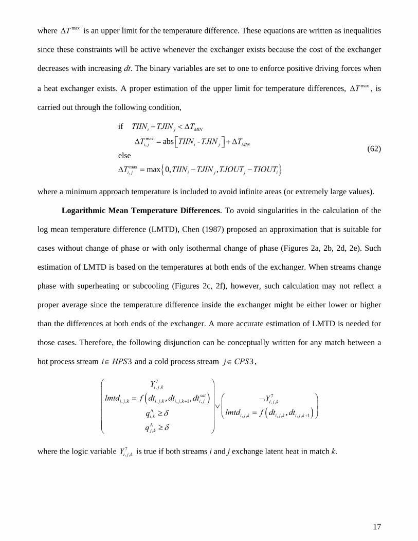
Logarithmic Mean Temperature Differences. To avoid singularities in the calculation of the

log mean temperature difference (LMTD), Chen (1987) proposed an approximation that is suitable for

cases without change of phase or with only isothermal change of phase (Figures 2a, 2b, 2d, 2e). Such

estimation of LMTD is based on the temperatures at both ends of the exchanger. When streams change

phase with superheating or subcooling (Figures 2c, 2f), however, such calculation may not reflect a

proper average since the temperature difference inside the exchanger might be either lower or higher

than the differences at both ends of the exchanger. A more accurate estimation of LMTD is needed for

those cases. Therefore, the following disjunction can be conceptually written for any match between a

hot process stream 3i HPS∈ and a cold process stream 3j CPS∈ ,

( )( )

7, ,

7, , , , , , 1 , , ,

, , , , , , 1,

,

, ,

,

i j k

sati j k i j k i j k i j i j k

i j k i j k i j ki k

j k

Y

lmtd f dt dt dt Y

lmtd f dt dtq

q

δ

δ

+

Λ+

Λ

⎛ ⎞⎜ ⎟

= ⎛ ⎞¬⎜ ⎟⎜ ⎟∨⎜ ⎟ ⎜ ⎟=≥⎜ ⎟ ⎝ ⎠

⎜ ⎟⎜ ⎟≥⎝ ⎠

where the logic variable 7, ,i j kY is true if both streams i and j exchange latent heat in match k.

18

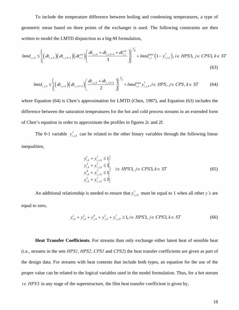
To include the temperature difference between boiling and condensing temperatures, a type of

geometric mean based on three points of the exchanger is used. The following constraints are then

written to model the LMTD disjunction as a big-M formulation,

( )( )( ) ( )1

4, , , , 1 , max 7

, , , , , , 1 , , , ,1 , 3, 3,3

sati j k i j k i jsat

i j k i j k i j k i j i j i j k

dt dt dtlmtd dt dt dt lmtd y i HPS j CPS k ST+

+

⎧ ⎫⎛ ⎞+ +⎪ ⎪≤ + − ∈ ∈ ∈⎜ ⎟⎨ ⎬⎜ ⎟⎪ ⎪⎝ ⎠⎩ ⎭ (63)

( )( )1

3, , , , 1 max 7

, , , , , , 1 , , , , , ,2

i j k i j ki j k i j k i j k i j i j k

dt dtlmtd dt dt lmtd y i HPS j CPS k ST+

+

⎧ + ⎫⎛ ⎞⎪ ⎪≤ + ∈ ∈ ∈⎨ ⎬⎜ ⎟⎪ ⎪⎝ ⎠⎩ ⎭

(64)

where Equation (64) is Chen’s approximation for LMTD (Chen, 1987), and Equation (63) includes the

difference between the saturation temperatures for the hot and cold process streams in an extended form

of Chen’s equation in order to approximate the profiles in figures 2c and 2f.

The 0-1 variable 7,, kjiy can be related to the other binary variables through the following linear

inequalities,

1 7, , ,2 7, , ,4 7, , ,

5 7, , ,

11

3, 3,11

i k i j k

i k i j k

i k i j k

i k i j k

y yy y

i HPS j CPS k STy yy y

⎫+ ≤⎪+ ≤ ⎪ ∈ ∈ ∈⎬+ ≤ ⎪⎪+ ≤ ⎭

(65)

An additional relationship is needed to ensure that 7,, kjiy must be equal to 1 when all other y’s are

equal to zero,

1 2 4 5 7, , , , , , 1, 3, 3,i k i k j k j k i j ky y y y y i HPS j CPS k ST+ + + + ≥ ∈ ∈ ∈ (66)

Heat Transfer Coefficients. For streams than only exchange either latent heat of sensible heat

(i.e., streams in the sets HPS1, HPS2, CPS1 and CPS2) the heat transfer coefficients are given as part of

the design data. For streams with heat contents that include both types, an equation for the use of the

proper value can be related to the logical variables used in the model formulation. Thus, for a hot stream

3i HPS∈ in any stage of the superstructure, the film heat transfer coefficient is given by,

19

( )1 2 1 2, , , , ,1 , 3,suph subc mean

i k i i k i i k i i k i kh h y h y h y y i HPS k ST= + + − − ∈ ∈ (67)

whereas for a match of a hot stream with a cold utility,

( )3 31 , 3cu subc meani i i i ih h y h y i HPS= + − ∈ (68)

where

( ) ( )( ) ( )

, 3suph cond subc cond cond condi i i i i i i i i imean

i cond cond condi i i i i i i

h FCP TIN T h FCP T TOUT h Fh i HPS

FCP TIN T FCP T TOUT F

λ

λ

− + − += ∈

− + − + (69)

Note from (67) that for streams that are either above or below saturation the inlet heat transfer

coefficient reduces to either hihsup or subc

ih . For the case where phase change is included meanih represents

an average heat transfer coefficient weighted by corresponding heat content contributions.

Similarly, for a cold stream 3j CPS∈ ,

( )5 4 4 5, , , , ,1 , 3,suph subc mean

j k j j k j j k j j k j kh h y h y h y y j CPS k ST= + + − − ∈ ∈ (70)

and for a match with a hot utility,

( )6 61 , 3hu suph meanj j j j jh h y h y j CPS= + − ∈ (71)

where,

( ) ( )( ) ( )

, 3suph evap subc evap evap evapj j j j j j j j j jmean

j evap evap evapj j j j j j j

h FCP TOUT T h FCP T TIN h Fh j CPS

FCP TOUT T FCP T TIN F

λ

λ

− + − += ∈

− + − + (72)

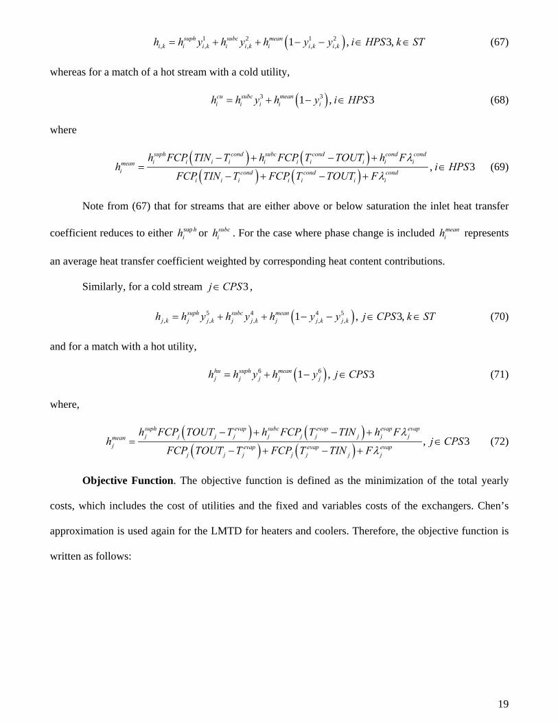
Objective Function. The objective function is defined as the minimization of the total yearly

costs, which includes the cost of utilities and the fixed and variables costs of the exchangers. Chen’s

approximation is used again for the LMTD for heaters and coolers. Therefore, the objective function is

written as follows:

20

( )

, , , , ,

, ,, ,

,, ,

,

,

min

1 1

1 1

i ji HPS j CPS

i j j k i cu i cu j ji HPS j CPS k ST i HPS j CPS

i j ki k j k

i ji HPS j CPS k ST i j k

i cui cu

i cu

i cu

CCUqcu CHUqhu

CF z CF zcu CF zhu

qh h

Clmtd

qcuh h

C

dt TOU

β

δ

∈ ∈

∈ ∈ ∈ ∈ ∈

∈ ∈ ∈

+

+ + +

⎧ ⎫⎛ ⎞+⎪ ⎪⎜ ⎟⎜ ⎟⎪ ⎪⎝ ⎠+ ⎨ ⎬+⎪ ⎪

⎪ ⎪⎩ ⎭

⎛ ⎞+⎜ ⎟

⎝ ⎠+

∑ ∑

∑ ∑ ∑ ∑ ∑

∑ ∑ ∑

( )

( )( )

13

,

,

, 13

,,

2

1 1

2

i HPSi cu i cu

i cu

hu j huhu j

hu jj CPS

hu j hu jhu j hu j

dt TOUT TINT TIN

qh h

Cdt TIN TOUT

dt TIN TOUT

β

β

δ

δ

∈

∈

⎧ ⎫⎪ ⎪⎪ ⎪⎨ ⎬⎪ ⎪⎡ + − ⎤⎛ ⎞

− +⎪ ⎪⎢ ⎥⎜ ⎟⎝ ⎠⎣ ⎦⎩ ⎭

⎧ ⎫⎛ ⎞⎪ ⎪+⎜ ⎟⎜ ⎟⎪ ⎪⎪ ⎪⎝ ⎠+ ⎨ ⎬⎪ ⎪⎡ + − ⎤⎛ ⎞

− +⎪ ⎪⎢ ⎥⎜ ⎟⎝ ⎠⎪ ⎪⎣ ⎦⎩ ⎭

∑

∑

(73)

In summary, the proposed MINLP model for the HEN synthesis including isothermal and non-

isothermal streams consists of the minimization of equation (73), subject to the constraints given by

equations (1-72). The continuous variables (t, q, dt, lmtd, h, qΛ) are nonnegative, and z and y are sets of

binary variables.

Remarks

1) In the MINLP model the objective function is nonlinear and all the constraints are linear,

except for equations (63) and (64) for the logarithmic mean temperature differences.

2) Notice that the overall energy balance for streams that transfer only sensible heat (Equations

(1) and (4)) are linearly dependent, because they can be obtained by combining the energy balances for

each stage (Equations (7) and (9)) and the energy balances for utilities (Equations (19) and (21)).

Although they have been written here for the sake of completeness, Equations (1) and (4) can be

therefore removed of the model. A similar observation applies for Equations (3) and (6). The overall

energy balance for pure isothermal streams (i.e., streams that only exchange latent heat), however, are

needed in the model because energy balances for each stage are not written for these types of streams.

21

3) For nonisothermal streams that require splitting, isothermal mixing at the end of a stage is

used as a simplifying assumption in the model (as in Yee and Grossmann, 1990). On the other hand,

isothermal mixing is a natural consequence for a split stream with change of phase, and in that case the

heat exchangers can be placed either in series or in parallel. For the general case one can use the two-

stage procedure by Yee and Grossmann to obtain unequal outlet temperatures of split streams.

4) The model for streams with change of phase is strictly correct for pure components. For

multicomponent mixtures, an approximation such that the bubble and dew temperatures are the same is

made.

4. Examples

Five case studies are presented to show the application of the proposed algorithm. In the

examples the capital cost function for the heat exchangers was given by $1,650 (A)0.65 (A in m2), and an

annuity factor of 0.23 yr-1 was used. The unit costs for the heating and cooling utilities were assumed as

100 $/kW year and 10 $/kW year, respectively. A value of ΔTMIN of 5°K was used for all the examples.

The solver DICOPT included in the general algebraic modeling system GAMS (Brooke et al., 2006)

was used for the solution of the problems.

Example 1

This is a fairly simple problem that serves as a motivational example, in which only isothermal

streams are considered. Table 1 gives the stream data for two hot and two cold process streams, along

with heating and cooling utilities. Figure 10 shows the composite curves for this problem. Notice that

for these types of examples the composite curves may overlap even when the minimum temperature

difference is not reached.

For this simple problem, the original Synheat model proposed by Yee and Grossmann (1990)

was unable to get a feasible solution. That model approximates isothermal streams using a one degree

temperature change with a suitable (generally large) value of the heat capacity that matches the total

22

heat content of that stream. The main difficulty of this procedure has to do with scaling problems.

Another difficulty of the Synheat model for these types of problems is the proposed value for the

parameter max,i jTΔ ; such a model uses the following equation to calculate the upper limit for the

temperature difference,

{ }max, max 0, ,i j i j j iT TIIN TJIN TJOUT TIOUTΔ = − − (74)

Equation (74) works properly for non isothermal streams, but for the case of isothermal streams

it can lead to errors. For example, considering the data given in Table 1 and a match between hot stream

H1 and cold stream C1, the parameter max,i jTΔ given by Equation (74) is equal to 10. From the original

design data, the difference tik – tjk is -10, such that the match between streams H1 and C1 should not be

allowed by the model. If the binary variable is zero, then the right hand side of Equation (58),

max1, 1, 1,1k kt t T− + Δ , becomes zero, which violates the value of ΔTMIN and therefore leads to an infeasible

solution from the original Synheat model even when the exchanger is not selected. Through the use of

equation (62) a proper bound for max,i jTΔ is estimated, and the model here presented provides an optimal

solution to this problem.

Table 1. Data for Example 1

stream TIN [K] TOUT [K] Fλ [KW] Type phasechangeT [K] h [KW/(m2 K)]

H1 400 400 4,000 HPS2 400 1.80 H2 425 425 3,000 HPS2 425 1.90 HU 627 627 - - - 2.50 C1 410 410 4,000 CPS2 410 1.70 C2 390 390 3,000 CPS2 390 1.85 CU 303 315 - - - 1.00

23

Figure 10. Composite curves for Example 1

Figure 11 shows the network obtained using the proposed model, which has a total yearly cost of

$142,629/year, with utility and annualized investment costs of $110,000/year and $32,629/year,

respectively. Note that this network achieves maximum energy recovery as shown in Figure 10.

Figure 11. Network obtained for Example 1

Example 2

The stream data for Example 2 are given in Table 2. The composite curves for this problem are

shown in Figure 1 for a HRAT of 5°K. This example consists of a set of streams with latent heat only,

24

and another set of streams with sensible heat only. Therefore, the model for this case does not include

the constraints for sets HPS3 and CPS3.

Table 2. Stream data for Example 2

stream TIN [K]

TOUT [K]

F [Kg/s]

Cp [KJ/(Kg K)] or λ [KJ/Kg]

FCp [KW/K] or Fλ [KW]

Type phasechangeT [K]

h [KW/(m2 K)]

H1 503 308 15.44 4.3 66.4 HPS1 - 0.81 H2 425 425 13.00 2,540.0 33,020.0 HPS2 425 1.78 H3 381 381 6.50 1,980.0 12,870.0 HPS2 381 1.62 HU 627 627 - - - - - 2.5 C1 323 503 11.69 4.2 49.1 CPS1 - 0.72 C2 408 408 9.98 1,845.0 18,413.1 CPS2 408 1.91 C3 391 391 7.97 2,321.0 18,498.4 CPS2 391 1.76 C4 353 353 7.24 2,258.0 16,347.9 CPS2 353 1.84 CU 303 315 - - - - - 1.00

Figure 12 shows the optimal network obtained using the proposed model, while Table 3 shows

the details for the heat exchangers of the network. The dashed lines in Figure 12 are used to denote the

isothermal streams. Nine units are required, out of which seven correspond to process-process

exchangers. The hot and cold utility costs are $510,639/year and $18,470/year, respectively, and the

investment cost for the heat exchangers is $157,905/year. The total yearly cost for the network is

$687,014/year.

Figure 12 shows a schematic representation of the temperature profiles for each of the heat

exchangers of the network. Notice that exchangers 2, 3 and 4 may be placed either in series or in

parallel for the hot process stream H2 (an isothermal stream). The same observation applies for

exchangers 1 and 4 for the cold process stream C3, and exchangers 5 and 6 for cold process stream C4.

25

H1

H2

H3

C1

C2

C3

503°

425°

381°

503°

408°

391°

308°

425°

381°

323°

408°

391°4

6

8

T

Q

Exchanger 1 and 6

T

Q

Exchangers 3, 4 and 5T

Q

Exchanger 2 and Heater 9

T

Q

Exchanger 7 and cooler 8

Temperature profiles for the exchangers

C4 353° 353°

1

1

2

5

2

3

9

410.4°

399°

7335.8°

3

7353°

353°

6358°

4

5

391°

kW

kW

kW

kW

kW kW

kW

kW

kW

Figure 12. Optimal network for Example 2

Table 3. Details for the units of Figure 12

Exchanger q [kW] A [m2] 1 6,150.0 212.2 2 2,258.6 97.6 3 18,413.1 1,175.6 4 12,348.3 410.4 5 12,870.0 533.5 6 3,477.9 297.8 7 1,473.0 465.8 8 1,847.0 374.0 9 5,106.4 53.5

26

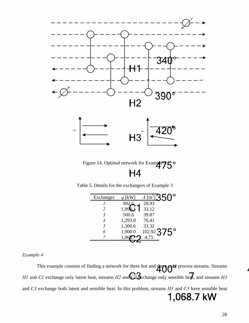
Example 3

Table 4 shows the stream data for Example 3, which consists of four hot and three cold process

streams. All process streams in this example are isothermal. Figure 13 shows the composite curves for

this case. It can be noticed that there is no pinch temperature if one takes the value of 5 °K as a

reference. For this example, the equations for the subsets HPS2 and CPS2 apply. The optimal network

obtained is shown in Figure 14. The lowest value of temperature differences among streams is 15 °K,

which is observed in exchanger 3. All streams are used for energy integration in the network, except for

stream H1, which must be fully processed with cooling utilities. Table 5 shows the data for the

exchangers of the network. The optimal solution shows utility and investment costs of $125,870/year

and $30,104/year, respectively, which yields a total annual cost of $155,974/year.

Table 4. Stream data for Example 3

stream TIN [K] TOUT [K] F [Kg/s] λ [KJ/Kg] Fλ [KW] Type phasechangeT [K]

h [KW/(m2 K)]

H1 340 340 0.80 2,375 1,900.0 HPS2 340 1.52 H2 390 390 0.79 1,890 1,493.1 HPS2 390 1.63 H3 420 420 1.20 2,162 2,594.4 HPS2 420 1.75 H4 475 475 0.82 2,438 1,999.1 HPS2 475 1.58 HU 627 627 - - - - - 2.50 C1 350 350 0.50 1,985 992.5 CPS2 350 1.81 C2 375 375 0.79 2,280 1,801.2 CPS2 375 1.72 C3 400 400 1.88 2,320 4,361.6 CPS2 400 1.64 CU 303 315 - - - - - 1.00

27

Figure 13. Composite curves for Example 3

28

T T


Table 5. Details for the exchangers of Example 3

Exchanger q [kW] A [m2] 1 992.5 28.93 2 1,999.1 33.12 3 500.6 39.87 4 1,293.8 76.41 5 1,300.6 33.32 6 1,900.0 102.92 7 1,068.7 4.75

Example 4

This example consists of finding a network for three hot and three cold process streams. Streams

H1 and C1 exchange only latent heat, streams H2 and C2 exchange only sensible heat, and streams H3

and C3 exchange both latent and sensible heat. In this problem, streams H3 and C3 have sensible heat

29

segments for both superheated and subcooled conditions, and film heat transfer coefficients for each

segment are included in the stream data (see Table 6).


stream TIN [K]

TOUT [K]

F [Kg/s]

Cp [KJ/(Kg

K)]

λ [KJ/Kg]

FCp [KW/K]

Fλ [KW]


h [KW/(m2 K)]

H1 590 380 11.31 3.9 - 44.109 - HPS1 - 0.53 H2 480 480 7.98 - 2,130 - 16,997.4 HPS2 480 1.80 H3 500 320 8.16 4.2 1,881 34.272 15,348.9 HPS3 400 [0.52;0.71;2.1]HU 627 627 - - - - - - - 2.5 C1 450 600 8.66 4.5 - 38.970 - CPS1 - 0.54 C2 452 452 5.33 - 2,251 - 11,997.8 CPS2 452 2.3 C3 310 550 6.42 3.7 1,725 23.754 11,074.5 CPS3 380 [0.62;0.80;1.9]CU 303 315 - - - - - - - 1.00

Figure 15 shows the optimum network obtained using the proposed model. One can observe how

in exchanger 4 both process streams H2 and C3 exchange sensible and latent heats; stream C3 enters the

exchanger at its supplied temperature (subcooled conditions) and exists as a superheated stream, while

stream H3 enters the exchanger at superheated conditions and exits with partial condensation. A cooler

(exchanger 8) is then needed to bring stream H3 from a mixture of vapor-liquid to a subcooled liquid.

Process stream H2 fully integrates stream C2 (exchanger 5) and requires the use of a cold utility to reach

its target conditions. In this problem the estimation of film heat transfer coefficients for streams with

multiple segments of heat transfer must be made. For stream H3, the mean coefficient in exchanger 4

and in cooler 8 (where both latent and sensible heats are processed) is 0.857 kW/m2 K, while for stream

C3 the film coefficient is 1.483 in exchanger 4 (both latent and sensible heat), and 0.62 in exchanger 2

and heater 10 (in which only sensible heat is exchanged).

Exchanger 4 integrates sensible and latent heats from both the hot and cold streams. The

calculated area with the proposed approximation of LMTD for those cases (Equation 63) is 1,175 m2,

which shows an error of 3.0 percent with respect to a more accurate calculation of the area that takes

into account the different segments of heat transferred by each stream (1,212 m2). With the use of a

30

single LMTD given by Chen’s approximation (Equation 64), the estimated area is 1,026 m2, which

represents an error of 15.3 percent. Thus, it is clear that Equation 64 provides very good approximations

to exchangers with sensible and latent heats.

One characteristic of the network is the many matches that are observed with the minimum

temperature difference. The optimal network for this example has heating and cooling costs of

$142,851/year and $145,885/year, respectively, and an investment cost of $167,411/year, yielding a

total yearly cost of $456,147/year.

31

H1

H2

C1

C2

C3

590°

480°

600°

452°

550°

380°

450°

452°

310°

2

2

9

5

5

3

3

4

4

71.0 m2

233.8 m2

424.5 m2

897.3 m2

1,175.3 m2

6500° 460.2°

7480°

H3500°

8320°

10

3.0 m2

480°

495°

95.0 m2

45.5 m2

312.7 m2

Exchanger 1

Q

Exchanger 2

Q

Exchanger 3

Q

Exchanger 4

Q

Exchanger 5

Q

Cooler 7

Q

Cooler 8

Q

Heater 9

Q

Heater 10

Q

H1

C1

H1

C3

H1

C1

H2

C3

H2

C2

H2

CU CU

H3

HU HU

C1

C3


400°

495°545°

1

1566.4°

873.7 m2

Cooler 6

Q

H1

CU


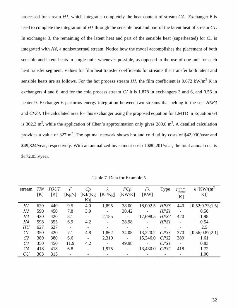
Example 5

The stream data for this example are shown in Table 7, in which process streams H1 and C1

must exchange both latent and sensible heat. This example also includes streams that exchange only

latent or sensible heat. Figure 16 shows the optimal network obtained for this case. Six internal

exchangers, two heaters and two coolers comprise the network. From the network structure and the

temperature profiles of Figure 16, one can see that in exchanger 4 both sensible and latent heats are

32

processed for stream H1, which integrates completely the heat content of stream C4. Exchanger 6 is

used to complete the integration of H1 through the sensible heat and part of the latent heat of stream C1.

In exchanger 3, the remaining of the latent heat and part of the sensible heat (superheated) for C1 is

integrated with H4, a nonisothermal stream. Notice how the model accomplishes the placement of both

sensible and latent heats in single units whenever possible, as opposed to the use of one unit for each

heat transfer segment. Values for film heat transfer coefficients for streams that transfer both latent and

sensible heats are as follows. For the hot process stream H1, the film coefficient is 0.672 kW/m2 K in

exchangers 4 and 6, and for the cold process stream C1 it is 1.878 in exchangers 3 and 6, and 0.56 in

heater 9. Exchanger 6 performs energy integration between two streams that belong to the sets HSP3

and CPS3. The calculated area for this exchanger using the proposed equation for LMTD in Equation 64

is 302.3 m2, while the application of Chen’s approximation only gives 289.8 m2. A detailed calculation

provides a value of 327 m2. The optimal network shows hot and cold utility costs of $42,030/year and

$49,824/year, respectively. With an annualized investment cost of $80,201/year, the total annual cost is

$172,055/year.


stream TIN [K]

TOUT [K]

F [Kg/s]

Cp [KJ/(Kg

K)]

λ [KJ/Kg]

FCp [KW/K]

Fλ [KW]


h [KW/(m2 K)]

H1 620 440 9.5 4.0 1,895 38.00 18,002.5 HPS3 440 [0.52;0.73;1.5]H2 590 450 7.8 3.9 - 30.42 - HPS1 - 0.58 H3 420 420 8.1 - 2,185 - 17,698.5 HPS2 420 1.98 H4 598 355 6.9 4.2 - 28.98 - HPS1 - 0.54 HU 627 627 - - - - - - - 2.5 C1 350 420 7.1 4.8 1,862 34.08 13,220.2 CPS3 370 [0.56;0.87;2.1]C2 380 380 6.6 - 2,310 - 15,246.0 CPS2 380 1.61 C3 350 450 11.9 4.2 - 49.98 - CPS1 - 0.83 C4 418 418 6.8 - 1,975 - 13,430.0 CPS2 418 1.72 CU 303 315 - - - - - - - 1.00

33

H1

H2

C1

C2

C3

620°

590°

420°

380°

450°

440°

350°

380°

350°

2

1

9

1

2

6

6

5

1.7 m2

108.1 m2

429.4 m2

302.3 m2

12.9 m2

440°

7

450°

H3420°

8

420°

10

2.2 m2

370°

26.6 m2

95.3 m2

Exchanger 1

Q

Exchanger 2

Q

Exchanger 3

Q

Exchanger 4

Q

Exchanger 5

Q

Cooler 7

Q

Cooler 8

Q

Heater 9

Q

Heater 10

Q

H2

C3

H3

C2

H4

C1

H1

C4

H3

C3

H3

CUCU

H4 HU HU

C1C3


420°

359.8°445°

4

3415°

73.5 m2

Exchanger 6

Q

H1

C1

5420°

3598°H4

355°

C4418°

4418°

350.7 m2

459.2°

Figure 16. Optimal networks for Example 5

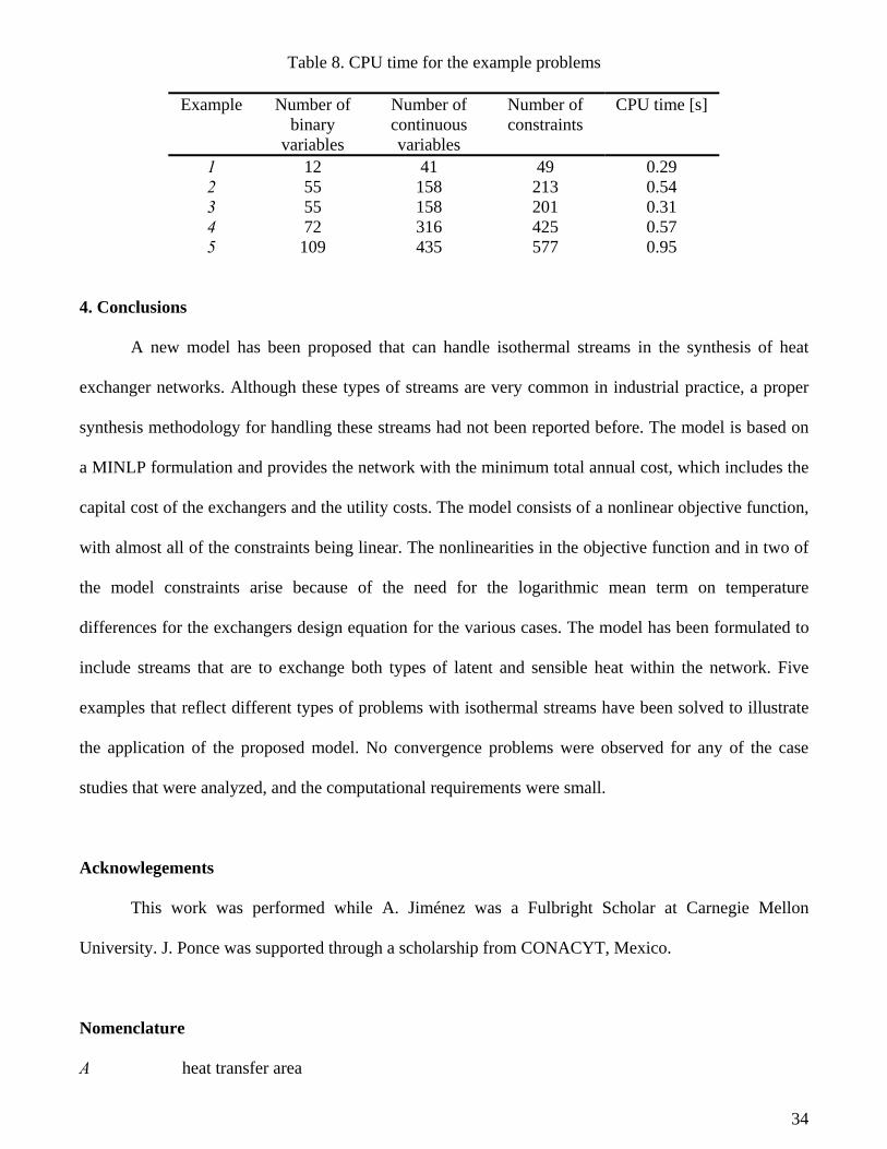
Finally, we report the sizes and computer times needed to obtain the optimal solutions. Table 8

shows the CPU time for the example problems, run with DICOPT under a Pentium 4 system with 2.66

GHz. It can be observed how the solution to the cases of study here presented was readily obtained

using the proposed model.

34

Table 8. CPU time for the example problems

Example Number of binary

variables

Number of continuous variables

Number of constraints

CPU time [s]

1 12 41 49 0.29 2 55 158 213 0.54 3 55 158 201 0.31 4 72 316 425 0.57 5 109 435 577 0.95

4. Conclusions

A new model has been proposed that can handle isothermal streams in the synthesis of heat

exchanger networks. Although these types of streams are very common in industrial practice, a proper

synthesis methodology for handling these streams had not been reported before. The model is based on

a MINLP formulation and provides the network with the minimum total annual cost, which includes the

capital cost of the exchangers and the utility costs. The model consists of a nonlinear objective function,

with almost all of the constraints being linear. The nonlinearities in the objective function and in two of

the model constraints arise because of the need for the logarithmic mean term on temperature

differences for the exchangers design equation for the various cases. The model has been formulated to

include streams that are to exchange both types of latent and sensible heat within the network. Five

examples that reflect different types of problems with isothermal streams have been solved to illustrate

the application of the proposed model. No convergence problems were observed for any of the case

studies that were analyzed, and the computational requirements were small.

Acknowlegements

This work was performed while A. Jiménez was a Fulbright Scholar at Carnegie Mellon

University. J. Ponce was supported through a scholarship from CONACYT, Mexico.

Nomenclature

A heat transfer area

35

C area cost coefficient

CCU unit cost of cold utility

CHU unit cost of hot utility

CF fixed charge for exchangers

Cp specific heat capacity

CPS {j | j is a cold process stream}

CPS1 {j | j is a non isothermal cold process stream}

CPS2 {j | j is an isothermal cold process stream}

CPS3 {j | j is a stream that exchanges latent and sensible heat}

CU cold utility

dti,j,k temperature approach difference for match (i,j) at temperature location k

dtcui temperature approach difference for match between hot stream i and a cold utility

dthuj temperature approach difference for match between cold stream j and a hot utility

,sati jdt temperature difference between saturated streams

F flow rate

FCp heat capacity flow rate

h fouling heat transfer coefficient

condh fouling heat transfer coefficient for condensation

evaph fouling heat transfer coefficient for evaporation

meanh mean fouling heat transfer coefficient

suphh fouling heat transfer coefficient for superheated part of a stream

subch fouling heat transfer coefficient for subcooled part of a stream

HPS {i | i is a hot process stream}

HPS1 {i | i is a non isothermal hot process stream}

HPS2 {i | i is an isothermal hot process stream}

36

HPS3 {i | i is a stream that exchange latent and sensible heat}

HU hot utility

lmtdi,j,k log-mean temperature difference

max,i jlmtd upper limit for the lmtd for match i,j

NOK total number of stages

qi,j,k heat exchanged between hot process stream i and cold process stream j in stage k

qcui heat exchanged between cold utility and hot stream i

qhuj heat exchanged between hot utility and cold stream j

maxQ upper bound for heat exchange

ST {k | k is a stage in the superstructure, k = 1, …, NOK}

ti,k temperature of hot stream i at the hot end of stage k

tj,k temperature of cold stream j at the hot end of stage k

,ni kt disaggregated variables used to model disjunctions

,nj kt disaggregated variables used to model disjunctions

Ticond condensation temperature for hot stream i

Tjevap evaporation temperature for cold stream j

phasechangeT phase change temperature

TINi inlet temperature of stream i

TOUTi outlet temperature of stream i

maxTΔ upper bound for temperature difference

ΔTMIN minimum approach temperature difference

Y boolean variables used to model disjunctions

y binary variables used to model disjunctions

zi,j,k binary variables for match (i,j) in stage k

zcui binary variables for match between cold utility and hot stream i

37

zhuj binary variables for match between hot utility and cold stream j

Greek Symbols

λ unit latent heat

Fλicond condensation heat load for hot stream i

Fλjevap evaporation heat load for cold stream j

,i kqΛ condensation heat load of hot stream i exchanged at stage k

,j kqΛ evaporation heat load of cold stream j exchanged at stage k

,cuiqΛ condensation heat load that is exchanged with the cold utility

,hujqΛ evaporation heat load exchanged with a hot utility

β exponent for area in cost equation

δ small number

Subscripts

i hot process stream

j cold process stream

k index for stage (1, …, NOK) and temperature location (1, …, NOK+1)

References

Brooke, A., Kendrick, D., Meeruas, A., & Raman, R. (2006). GAMS-Language guide. Washington,

D.C.: GAMS Development Corporation.

Castier, M., & Queiroz, E.M. (2002). Energy targeting in heat exchanger network synthesis using

rigorous physical property calculations. Industrial and Engineering Chemistry Research. 41, 1511-1515.

38

Cerda, J., Westerberg, A.W., Mason, D., & Linnhoff, B. (1983) Minimum utility usage in heat

exchanger network synthesis – A transportation problem. Chemical Engineering Science. 38(3), 373-

387.

Chen, C.L., & Hung, P.S. (2004). Simultaneous synthesis of flexible heat-exchange networks with

uncertain source-stream temperatures and flow rates. Industrial and Engineering Chemistry Research.

43(18), 5916-5928.

Duran M.A., & Grossmann, I.E. (1986). Simultaneous optimization and heat integration of chemical

process. American Institute of Chemical Engineering Journal. 32, 123-138.

Furman, K.C., & Sahinidis, N.V. (2002). A critical review and annotated bibliography for heat

exchanger network synthesis in the 20th century. Industrial and Engineering Chemistry research. 41,

2335-2370.

Frausto-Hernandez, S., Rico-Ramirez, V., Jiménez-Gutiérrez, A., & Hernandez-Castro, S. (2003).

MINLP synthesis of heat exchanger networks considering pressure drop effects. Computers and

Chemical Engineering. 27, 1143-1152.

Grossmann, I.E., Yeomans, H., & Kravanja, Z. (1998). A rigorous disjunctive optimization model for

simultaneous flowsheet optimization and heat integration. Computers and Chemical Engineering. 22,

suppl, s157-s164.

Konukman, A.E.S., Camurdan, M.C., & Akman, U. (2002). Simultaneous flexibility targeting and

synthesis of minimum-utility heat-exchange networks with superstructure-based MILP formulation.

Chemical Engineering and Processing. 41(6), 501-518.

Linnhoff, B., & Flower, J.R. (1978). Synthesis of heat exchanger networks –I Systematic generation of

energy optimal networks. American Institute of Chemical Engineering Journal. 24(4), 633-642.

Linnhoff, B., & Hindmarsh, E. (1983). The pinch design method for head exchanger networks.

Chemical Engineering Science. 38(5), 745-763.

Liporace, F.S., Pessoa, F.L.P., & Queiroz, E.M. (2004). Heat exchanger network synthesis considering

change phase streams. Thermal Engineering. 3(2), 87-95.

39

Ma, K.L., Hui, C.W., & Yee T.F. (2000). Constant approach temperature model for HEN retrofit.

Applied Thermal Engineering. 20, 1505-1533.

Mizutani, F.T., Pessoa F.L.P., Queiroz, E.M., Hauan, S., & Grossmann I.E. (2003). Mathematical

programming model for heat-exchanger network synthesis including detailed heat-exchanger designs. 2.

Networks synthesis. Industrial and Engineering Chemistry Research. 42(17), 4019-4027.

Papoulias, S.A., & Grossmann, I.E. (1983). A structural optimization approach in process synthesis. 1.

Utility systems. Computers and Chemical Engineering, 7(6), 695-706.

Raman, R., & Grossmann, I.E. (1994). Modeling and computational techniques for logic based integer

programming. Computers and Chemical Engineering. 18, 563-578.

Serna-González, M., Ponce-Ortega, J.M., & Jiménez-Gutiérrez, A. (2004). Two-level optimization

algorithm for heat exchanger networks including pressure drop considerations. Industrial and

Engineering Chemistry Research. 43(21), 6766-6773.

Sorsak, A., & Kravanja, Z. (2004). MINLP retrofit of heat exchanger networks comprising different

exchanger types. Computers and Chemical Engineering. 28, 235-251.

Verheyen, W., & Zhang, N. (2006). Design of flexible heat exchanger network for multi-period

operation. Chemical Engineering Science. 61, 7730-7753.

Yee, T.F., & Grossmann, I.E. (1990). Simultaneous optimization model for heat integration –II Heat

exchanger network synthesis. Computers and Chemical Engineering. 14, 1165-1184.

optimal synthesis of heat exchanger networks involving...

Documents