optimal transmission network topology for...

- 1 -

Optimal Transmission Network Topology for Resilient Power Supply

Y. Zinchenko 1, H. Song

1, W. Rosehart

1

1 University of Calgary, Calgary, Canada

{[email protected], [email protected], [email protected]}

Abstract. An electric power supplier needs to build a transmission line between two jurisdictions.

Ideally, the design of the new electric power line would be such that it maximizes some user-defined

utility function, for example, minimizes the construction cost or the environmental impact. Due to

reliability considerations, the power line developer has to install not just one, but two transmission

lines, separated by a certain distance from one-another, so that even if one of the lines fails, the end

user will still receive electricity along the second line. In other words, the optimal placement of the

transmission lines corresponds to the topological design of a specialized unorthodox “supply chain”,

where the multiple power lines serve towards the system’s resilience against catastrophic failures. We

discuss how such a problem can be modeled, and in particular, demonstrate a setting that allows to

solve the problem efficiently, in polynomial time.

Keywords: power-line design, optimal topology, shortest path.

1 Introduction

Catastrophic changes in the operational and natural environments present a huge risk and uncertainty

in supply chains. Obviously, if one could easily predict such catastrophic outcomes, these events would

not cause an issue in most cases. However, in many situations our only option now is to build some

redundancy into the system, as is the case in power transmission. A natural question arises: how to add

the necessary level of redundancy at a least possible cost?

In many applications a necessity arises to determine a set of alternative paths between some origin and

a destination. For example, network robustness in the context of transit design was investigated in [12]; in

[13, 14, 15] several groups of authors study survivability of low cost communication networks, etc. Some

of the proposed models fall within the domain of the so-called bilevel programming, while others pursue

graph-theoretic approach. In this paper we follow the latter framework, and investigate a specific variant

of the shortest path type problem arising in power transmission line topology design. Transmission line

routing and planning has long drawn attention as an application for the shortest path; see for example [2-

7]. Much work in the literature focuses on expansion planning, where as route section is well documented

by transmission owners or regulators, for example [8-11]. Various reliability aspects of power systems are

well covered in the literature, for example see [16, 17]. In turn, the optimal placement of the transmission

lines corresponds to the topological design of a very specialized unorthodox “supply chain”, where the

multiple power lines serve towards the system’s resilience against catastrophic failures.

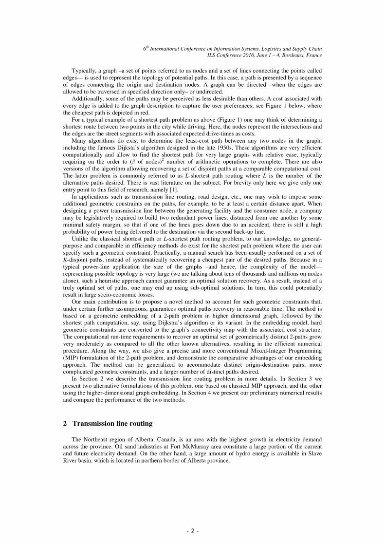
Figure 1: An example of a shortest path.

- 2 -

6th International Conference on Information Systems, Logistics and Supply Chain

ILS Conference 2016, June 1 – 4, Bordeaux, France

Typically, a graph –a set of points referred to as nodes and a set of lines connecting the points called

edges— is used to represent the topology of potential paths. In this case, a path is presented by a sequence

of edges connecting the origin and destination nodes. A graph can be directed –when the edges are

allowed to be traversed in specified direction only– or undirected.

Additionally, some of the paths may be perceived as less desirable than others. A cost associated with

every edge is added to the graph description to capture the user preferences; see Figure 1 below, where

the cheapest path is depicted in red.

For a typical example of a shortest path problem as above (Figure 1) one may think of determining a

shortest route between two points in the city while driving. Here, the nodes represent the intersections and

the edges are the street segments with associated expected drive-times as costs.

Many algorithms do exist to determine the least-cost path between any two nodes in the graph,

including the famous Dijksta’s algorithm designed in the late 1950s. These algorithms are very efficient

computationally and allow to find the shortest path for very large graphs with relative ease, typically

requiring on the order to (# of nodes)2 number of arithmetic operations to complete. There are also

versions of the algorithm allowing recovering a set of disjoint paths at a comparable computational cost.

The latter problem is commonly referred to as L-shortest path routing where L is the number of the

alternative paths desired. There is vast literature on the subject. For brevity only here we give only one

entry point to this field of research, namely [1].

In applications such as transmission line routing, road design, etc., one may wish to impose some

additional geometric constraints on the paths, for example, to be at least a certain distance apart. When

designing a power transmission line between the generating facility and the consumer node, a company

may be legislatively required to build two redundant power lines, distanced from one another by some

minimal safety margin, so that if one of the lines goes down due to an accident, there is still a high

probability of power being delivered to the destination via the second back-up line.

Unlike the classical shortest path or L-shortest path routing problem, to our knowledge, no general-

purpose and comparable in efficiency methods do exist for the shortest path problem where the user can

specify such a geometric constraint. Practically, a manual search has been usually performed on a set of

K-disjoint paths, instead of systematically recovering a cheapest pair of the desired paths. Because in a

typical power-line application the size of the graphs –and hence, the complexity of the model—

representing possible topology is very large (we are talking about tens of thousands and millions on nodes

alone), such a heuristic approach cannot guarantee an optimal solution recovery. As a result, instead of a

truly optimal set of paths, one may end up using sub-optimal solutions. In turn, this could potentially

result in large socio-economic losses.

Our main contribution is to propose a novel method to account for such geometric constraints that,

under certain further assumptions, guarantees optimal paths recovery in reasonable time. The method is

based on a geometric embedding of a 2-path problem in higher dimensional graph, followed by the

shortest path computation, say, using Dijkstra’s algorithm or its variant. In the embedding model, hard

geometric constraints are converted to the graph’s connectivity map with the associated cost structure.

The computational run-time requirements to recover an optimal set of geometrically distinct 2-paths grow

very moderately as compared to all the other known alternatives, resulting in the efficient numerical

procedure. Along the way, we also give a precise and more conventional Mixed-Integer Programming

(MIP) formulation of the 2-path problem, and demonstrate the comparative advantages of our embedding

approach. The method can be generalized to accommodate distinct origin-destination pairs, more

complicated geometric constraints, and a larger number of distinct paths desired.

In Section 2 we describe the transmission line routing problem in more details. In Section 3 we

present two alternative formulations of this problem, one based on classical MIP approach, and the other

using the higher-dimensional graph embedding. In Section 4 we present our preliminary numerical results

and compare the performance of the two methods.

2 Transmission line routing

The Northeast region of Alberta, Canada, is an area with the highest growth in electricity demand

across the province. Oil sand industries at Fort McMurray area constitute a large portion of the current

and future electricity demand. On the other hand, a large amount of hydro energy is available in Slave

River basin, which is located in northern border of Alberta province.

- 3 -



The problem is how to transmit generated electricity to the Fort McMurray area. The northern region

has a very sparse population and most of the area is covered with forests and ice, while there is almost no

human development in the area. The hydro-generated power has to be transmitted via power lines to

substations in the vicinity of oil sand facilities in Fort McMurray. Through this, it is possible to bring

green energy to energy intensive oil sand operations and contribute to greenhouse gas reduction plans.

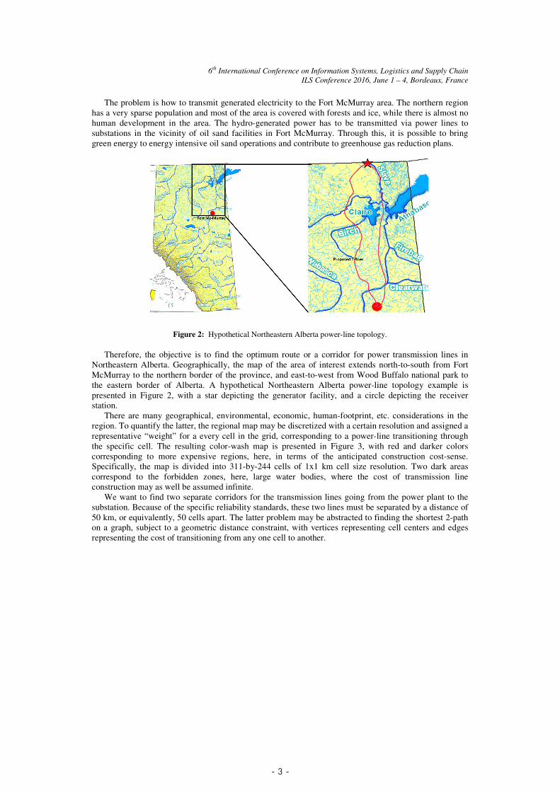
Figure 2: Hypothetical Northeastern Alberta power-line topology.

Therefore, the objective is to find the optimum route or a corridor for power transmission lines in

Northeastern Alberta. Geographically, the map of the area of interest extends north-to-south from Fort

McMurray to the northern border of the province, and east-to-west from Wood Buffalo national park to

the eastern border of Alberta. A hypothetical Northeastern Alberta power-line topology example is

presented in Figure 2, with a star depicting the generator facility, and a circle depicting the receiver

station.

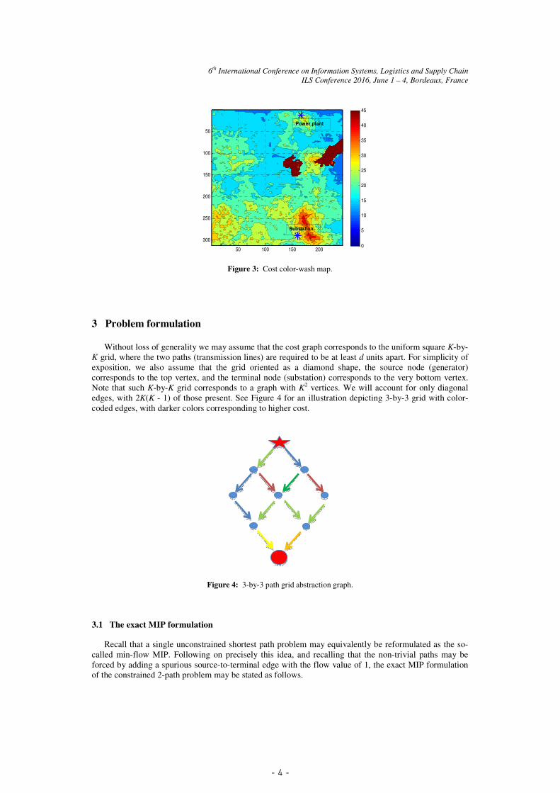
There are many geographical, environmental, economic, human-footprint, etc. considerations in the

region. To quantify the latter, the regional map may be discretized with a certain resolution and assigned a

representative “weight” for a every cell in the grid, corresponding to a power-line transitioning through

the specific cell. The resulting color-wash map is presented in Figure 3, with red and darker colors

corresponding to more expensive regions, here, in terms of the anticipated construction cost-sense.

Specifically, the map is divided into 311-by-244 cells of 1x1 km cell size resolution. Two dark areas

correspond to the forbidden zones, here, large water bodies, where the cost of transmission line

construction may as well be assumed infinite.

We want to find two separate corridors for the transmission lines going from the power plant to the

substation. Because of the specific reliability standards, these two lines must be separated by a distance of

50 km, or equivalently, 50 cells apart. The latter problem may be abstracted to finding the shortest 2-path

on a graph, subject to a geometric distance constraint, with vertices representing cell centers and edges

representing the cost of transitioning from any one cell to another.

- 4 -



50 100 150 200

50

100

150

200

250

300

0

5

10

15

20

25

30

35

40

45

Substation

Power plant

Figure 3: Cost color-wash map.

3 Problem formulation

Without loss of generality we may assume that the cost graph corresponds to the uniform square K-by-

K grid, where the two paths (transmission lines) are required to be at least d units apart. For simplicity of

exposition, we also assume that the grid oriented as a diamond shape, the source node (generator)

corresponds to the top vertex, and the terminal node (substation) corresponds to the very bottom vertex.

Note that such K-by-K grid corresponds to a graph with K2 vertices. We will account for only diagonal

edges, with 2K(K - 1) of those present. See Figure 4 for an illustration depicting 3-by-3 grid with color-

coded edges, with darker colors corresponding to higher cost.

Figure 4: 3-by-3 path grid abstraction graph.

3.1 The exact MIP formulation

Recall that a single unconstrained shortest path problem may equivalently be reformulated as the so-

called min-flow MIP. Following on precisely this idea, and recalling that the non-trivial paths may be

forced by adding a spurious source-to-terminal edge with the flow value of 1, the exact MIP formulation

of the constrained 2-path problem may be stated as follows.

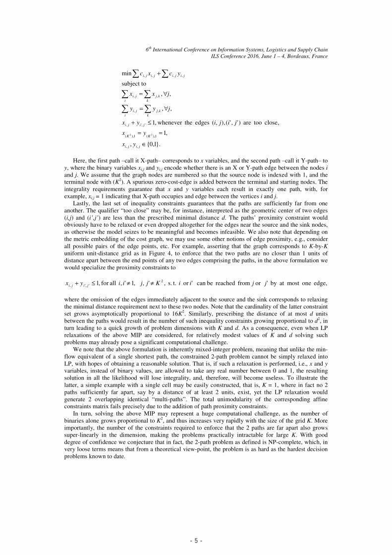
- 5 -



}.1,0{,

,1

close, tooare )','(),,( edges the whenever ,1

,,

,,

subject to

min

,,

1),(1),(

',',

,,

,,

,,,,

22

∈

==

≤+

∀=

∀=

+

jiji

KK

jiji

k

kj

i

ji

k

kj

i

ji

jijijiji

yx

yx

jijiyx

jyy

jxx

ycxc

Here, the first path –call it X-path– corresponds to x variables, and the second path –call it Y-path– to

y, where the binary variables xi,j and yi,j encode whether there is an X or Y-path edge between the nodes i

and j. We assume that the graph nodes are numbered so that the source node is indexed with 1, and the

terminal node with (K2). A spurious zero-cost-edge is added between the terminal and starting nodes. The

integrality requirements guarantee that x and y variables each result in exactly one path, with, for

example, xi,j = 1 indicating that X-path occupies and edge between the vertices i and j.

Lastly, the last set of inequality constraints guarantees that the paths are sufficiently far from one

another. The qualifier “too close” may be, for instance, interpreted as the geometric center of two edges

(i,j) and (i’,j’) are less than the prescribed minimal distance d. The paths’ proximity constraint would

obviously have to be relaxed or even dropped altogether for the edges near the source and the sink nodes,

as otherwise the model seizes to be meaningful and becomes infeasible. We also note that depending on

the metric embedding of the cost graph, we may use some other notions of edge proximity, e.g., consider

all possible pairs of the edge points, etc. For example, asserting that the graph corresponds to K-by-K

uniform unit-distance grid as in Figure 4, to enforce that the two paths are no closer than 1 units of

distance apart between the end points of any two edges comprising the paths, in the above formulation we

would specialize the proximity constraints to

edge, onemost at by 'or from reached becan 'or t.s. ,', ,1', allfor ,12

',', jjiiKjjiiyx jiji ≠≠≤+

where the omission of the edges immediately adjacent to the source and the sink corresponds to relaxing

the minimal distance requirement next to these two nodes. Note that the cardinality of the latter constraint

set grows asymptotically proportional to 16K2. Similarly, prescribing the distance of at most d units

between the paths would result in the number of such inequality constraints growing proportional to d2, in

turn leading to a quick growth of problem dimensions with K and d. As a consequence, even when LP

relaxations of the above MIP are considered, for relatively modest values of K and d solving such

problems may already pose a significant computational challenge.

We note that the above formulation is inherently mixed-integer problem, meaning that unlike the min-

flow equivalent of a single shortest path, the constrained 2-path problem cannot be simply relaxed into

LP, with hopes of obtaining a reasonable solution. That is, if such a relaxation is performed, i.e., x and y

variables, instead of binary values, are allowed to take any real number between 0 and 1, the resulting

solution in all the likelihood will lose integrality, and, therefore, will become useless. To illustrate the

latter, a simple example with a single cell may be easily constructed, that is, K = 1, where in fact no 2

paths sufficiently far apart, say by a distance of at least 2 units, exist, yet the LP relaxation would

generate 2 overlapping identical “multi-paths”. The total unimodularity of the corresponding affine

constraints matrix fails precisely due to the addition of path proximity constraints.

In turn, solving the above MIP may represent a huge computational challenge, as the number of

binaries alone grows proportional to K2, and thus increases very rapidly with the size of the grid K. More

importantly, the number of the constraints required to enforce that the 2 paths are far apart also grows

super-linearly in the dimension, making the problems practically intractable for large K. With good

degree of confidence we conjecture that in fact, the 2-path problem as defined is NP-complete, which, in

very loose terms means that from a theoretical view-point, the problem is as hard as the hardest decision

problems known to date.

- 6 -



3.2 Higher-dimensional embedding

As an alternative to the MIP formulation, we propose a much more efficient approximation approach

to finding the 2 disjoint paths, which under mild additional assumptions results in the exact solution. We

state these assumptions first.

(a) Let the vertical spacing between the vertices of the graph be such that the distance between the

paths can be judged solely by the horizontal distance between the visited nodes.

(b) Let the two paths be synchronous in vertical direction, that is, both paths be descending one

vertical step at a time.

With the above in mind, let us consider the following geometric embedding procedure. Firstly, let us

replicate the edge cost graph twice, and assign the graph realizations to two orthogonal plains, say XZ

and YZ. For each of the graph realizations, we align the corresponding Z axis with the line connecting the

source and destination nodes, while X and Y axis represent the orthogonal directions to Z. With two paths

in question being planar, one should think of X-path being embedded, or simply, depicted, in XZ plain,

and Y-path in YZ plain.

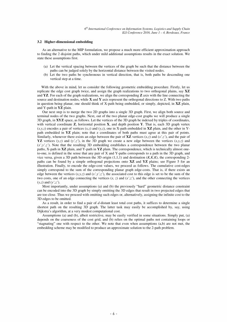
Our next step is to merge the two 2D graphs into a single 3D graph. First, we align both source and

terminal nodes of the two graphs. Next, out of the two planar edge-cost graphs we will produce a single

3D graph, in XYZ space, as follows. Let the vertices of the 3D graph be indexed by triples of coordinates,

with vertical coordinate Z, horizontal position X, and depth position Y. That is, each 3D graph vertex

(x,y,z) encodes a pair of vertices (x,z) and (y,z), one in X-path embedded in XZ plain, and the other in Y-

path embedded in YZ plain; note that z coordinates of both paths must agree at this pair of points.

Similarly, whenever there exists an edge between the pair of XZ vertices (x,z) and (x’,z’), and the pair of

YZ vertices (y,z) and (y’,z’), in the 3D graph we create a new edge between the vertices (x,y,z) and

(x’,y’,z’). Note that the resulting 3D embedding establishes a correspondence between the two planar

paths, X-path in XZ plain, and Y-path in YZ plain. The correspondence, which is technically almost one-

to-one, is defined in the sense that any pair of X and Y-paths corresponds to a path in the 3D graph, and

vice versa, given a 3D path between the 3D origin (1,1,1) and destination (K,K,K), the corresponding 2-

paths can be found by a simple orthogonal projections onto XZ and YZ plains; see Figure 5 for an

illustration. Finally, to encode the edge-cost values, we proceed as follows. The cumulative cost-edges

simply correspond to the sum of the corresponding planar graph edge-costs. That is, if there exists an

edge between the vertices (x,y,z) and (x’,y’,z’), the associated cost to this edge is set to be the sum of the

two costs, one of an edge connecting the vertices (x, z) and (x’,z’), and the other connecting the vertices

(y,z) and (y’,z’).

Most importantly, under assumptions (a) and (b) the previously “hard” geometric distance constraint

can be encoded into the 3D graph by simply omitting the 3D edges that result in two projected edges that

are too close. Thus we proceed with omitting such edges or, alternatively, assigning the infinite cost to the

3D edges to be omitted.

As a result, in order to find a pair of d-distant least total cost paths, it suffices to determine a single

shortest path on the resulting 3D graph. The latter task may easily be accomplished by, say, using

Dijkstra’s algorithm, at a very modest computational cost.

Assumptions (a) and (b), albeit restrictive, may be easily verified in some situations. Simply put, (a)

depends on the coarseness of the cost grid, and (b) relies on the optimal paths not containing loops or

“stagnating” one with respect to the other. We note that even when assumptions (a,b) are not met, the

embedding scheme may be modified to produce an approximate solution to the 2-path problem.

- 7 -



(a) (b)

Figure 5: 3D path embedding with K = 4 (a) and 2 paths as the subsequent projections (b), superimposed.

4 Preliminary models’ performance and discussion

Next, we briefly compare the performance of the two models. Both models are benchmarked using

Matlab environment. Since the MIP sizes grow very rapidly with the size of the grid K and the prescribed

minimal distance d, for simplicity and to give greater benefit of the doubt to the exact formulation, we

consider only the time required to solve the LP relaxation of the problem. In turn, it is reasonable to

expect that the MIP solution times cannot be any lower, if not far greater. For further equity of

comparison, in both cases of solving the relaxed MIP and the embedding models we use open source

solvers. Namely, in the former case of solving an LP relaxation we use the well-reputed SDPT3 conic

solver, while in the latter of solving a shortest path problem, we use the Dijkstra’s algorithm script freely

available from Mathworks/Matlab website.

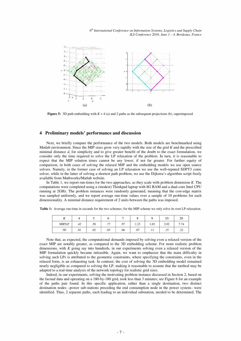
In Table 1, we report run-times for the two approaches, as they scale with problem dimension K. The

computations were completed using a (modest) Thinkpad laptop with 8G RAM and a dual-core Intel CPU

running at 2GHz. The problem instances were randomly generated, meaning that the cost-edge matrix

was sampled uniformly, and we report average run-time values over a sample of 10 problems for each

dimensionality. A minimal distance requirement of 2 units between the paths was imposed.

Table 1: Average run-time in seconds for the two schemes; for the MIP scheme we only solve its root LP relaxation.

K 4 5 6 7 8 9 10 20

MIP/LP .42 .58 .77 .97 1.23 1.65 2.02 7.74

3D .01 .02 .03 .06 .07 .11 .15 .22

Note that, as expected, the computational demands imposed by solving even a relaxed version of the

exact MIP are notably greater, as compared to the 3D embedding scheme. For more realistic problem

dimensions, with K going say into hundreds, in our experiments solving even a relaxed version of the

MIP formulation quickly became infeasible. Again, we want to emphasize that the main difficulty in

solving such LPs is attributed to the geometric constraints, where specifying the constraints, even in the

relaxed form, is an exhausting task. In contrast, the cost of solving the 3D embedding model remained

nearly negligible as compared to solving the LP, making it reasonable to assume that the method may be

adapted to a real-time analysis of the network topology for realistic grid sizes.

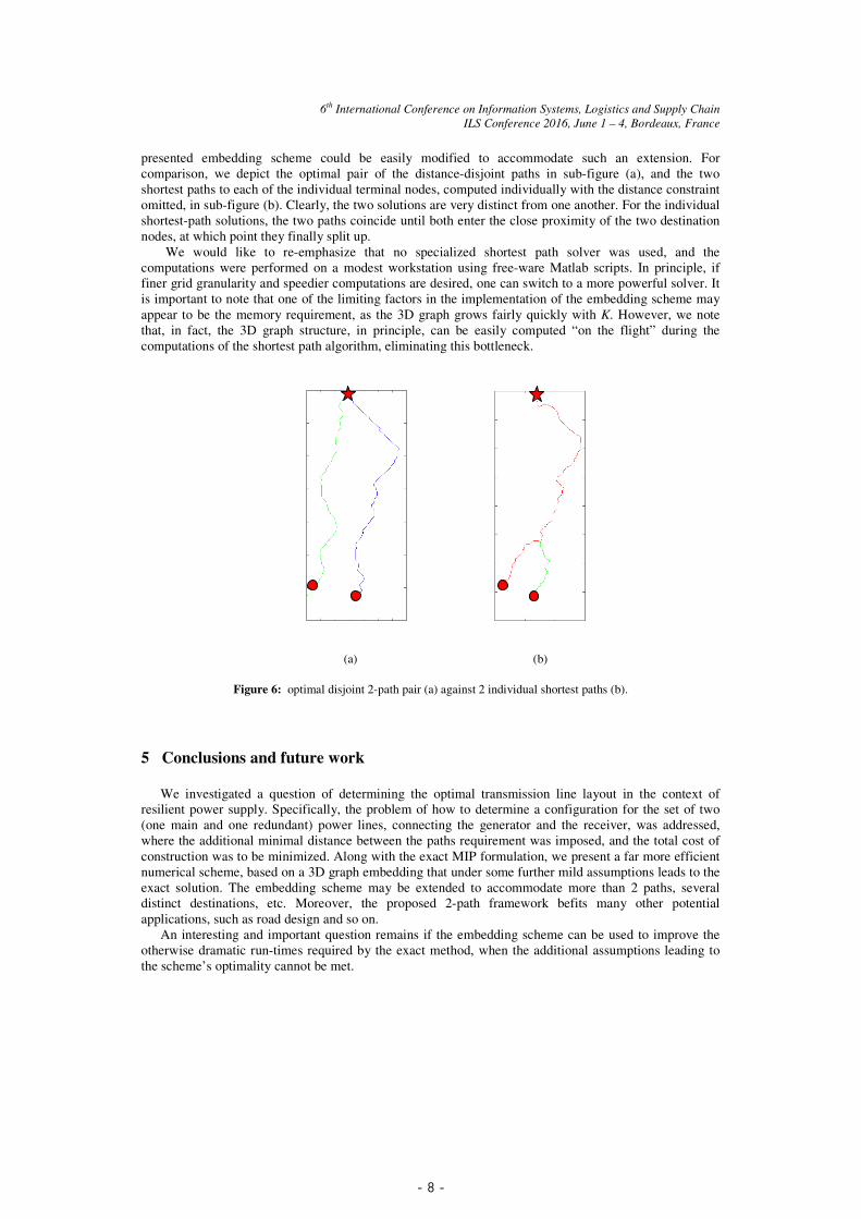
Indeed, in our experiments, solving the motivating problem instance discussed in Section 2, based on

the factual data and operating on a 180-by-180 grid, took less than 3 minutes; see Figure 6 for an example

of the paths pair found. In this specific application, rather than a single destination, two distinct

destination nodes –power sub-stations preceding the end consumption node in the power system– were

identified. Thus, 2 separate paths, each leading to an individual substation, needed to be determined. The

- 8 -



presented embedding scheme could be easily modified to accommodate such an extension. For

comparison, we depict the optimal pair of the distance-disjoint paths in sub-figure (a), and the two

shortest paths to each of the individual terminal nodes, computed individually with the distance constraint

omitted, in sub-figure (b). Clearly, the two solutions are very distinct from one another. For the individual

shortest-path solutions, the two paths coincide until both enter the close proximity of the two destination

nodes, at which point they finally split up.

We would like to re-emphasize that no specialized shortest path solver was used, and the

computations were performed on a modest workstation using free-ware Matlab scripts. In principle, if

finer grid granularity and speedier computations are desired, one can switch to a more powerful solver. It

is important to note that one of the limiting factors in the implementation of the embedding scheme may

appear to be the memory requirement, as the 3D graph grows fairly quickly with K. However, we note

that, in fact, the 3D graph structure, in principle, can be easily computed “on the flight” during the

computations of the shortest path algorithm, eliminating this bottleneck.

(a) (b)

Figure 6: optimal disjoint 2-path pair (a) against 2 individual shortest paths (b).

5 Conclusions and future work

We investigated a question of determining the optimal transmission line layout in the context of

resilient power supply. Specifically, the problem of how to determine a configuration for the set of two

(one main and one redundant) power lines, connecting the generator and the receiver, was addressed,

where the additional minimal distance between the paths requirement was imposed, and the total cost of

construction was to be minimized. Along with the exact MIP formulation, we present a far more efficient

numerical scheme, based on a 3D graph embedding that under some further mild assumptions leads to the

exact solution. The embedding scheme may be extended to accommodate more than 2 paths, several

distinct destinations, etc. Moreover, the proposed 2-path framework befits many other potential

applications, such as road design and so on.

An interesting and important question remains if the embedding scheme can be used to improve the

otherwise dramatic run-times required by the exact method, when the additional assumptions leading to

the scheme’s optimality cannot be met.

- 9 -



Acknowledgements

We would like to thank Sara Ghandehari Shandiz, PhD student, Department of Chemical and

Petroleum Engineering, and Joule Bergerson, Assistant Professor, Chemical and Petroleum Engineering,

for introducing a specific instance of a power line routing problem and providing a sample data set. Last,

but not least, we would like to sincerely thank the anonymous referees for the invaluable input that

hopefully led to an improved version of the manuscript.

References

1. Eppstein D.: Finding the k shortest paths. 35th IEEE Symp. Found. Comp. Sci., pp. 154-165. Santa Fe (1994)

2. El-Amin I., Al-Ghamdi F.: An expert system for transmission line route selection. Int. Power Engineering Conf,

vol. 2, Nanyang Technol. Univ, pp. 697–702. Singapore (1993)

3. Garver L.: Transmission network estimation using linear programming. Power Apparatus and Systems, IEEE

Transactions on, vol. PAS-89, pp. 1688-1697 (1970)

4. Cagigas C., Madrigal M.: Centralized vs. competitive transmission expansion planning: the need for new tools.

Power Engineering Society General Meeting IEEE, vol. 2, pp. 13-17 (2003)

5. Xie M., Zhong J., Wu F.: Multiyear transmission expansion planning using ordinal optimization. Power Systems,

IEEE Transactions on, vol. 22, pp. 1420 – 1428 (2007)

6. Monteiro C., Miranda V., Ramirez-Rosado I., Zorzano-Santamaria P., Garcia-Garrido E., Fernandez-Jimenez L.:

Compromise seeking for power line path selection based on economic and environmental corridors. IEEE

Transactions on Power Systems, pp. 1422-1430 (2005)

7. Shin J., Kim B., Park J., Lee K.: A new optimal routing algorithm for loss minimization and voltage stability

improvement in radial power systems. IEEE Transactions on Power Systems, vol. 22, pp. 636-657 (2007)

8. Altalink, Transmission Route Selection Process, accessed: June 15, 2015,

http://www.altalink.ca/valueoftransmission/route-selection-process.cfm

9. Great River Energy, 5.0 Transmission Line Route Selection Methodology, Accessed: June 15, 2015,

http://www.greatriverenergy.com/deliveringelectricity/currentprojects/aml_routeselectionmethodology.pdf

10. Manitoba-Minnesota Transmission Project – Route Selection Process; Accessed: June 15 2015,

https://www.hydro.mb.ca/projects/mb_mn_transmission/2014_r2_mmtp_siting_handout_web2.pdf

11. Donovan J., Sr. Vice President, Georgia Transmission Corporation: A national model for sitting transmission

lines. Electric Energy Online.com, Electric Energy T&D Magazine, July/August (2006)

12. Laporte G., Marín A., Mesa J. Perea F.: Designing robust rapid transit networks with alternative routes. Journal of

Advanced Transportation 45, pp. 54-65 (2011)

13. Fortz B., Labbe M.: Two-connected networks with rings of bounded cardinality. Computational Optimization and

Applications 27, pp. 123-148 (2004)

14. Fortz B., Mahjoub A., McCormick S., Pesneau P.: Two-edge connected subgraphs with bounded rings:

polyhedral results and branch-and-cut. Mathematical Programming 105, pp. 85-111 (2006)

15. Grotschel M,. Monma C., Stoer M.: Polyhedral and computational investigations for designing communication

networks with high survivability requirements. Operations Research 43, pp. 1012-1024 (1995)

16. Billinton R., Allan R. Reliability evaluation of power systems. Springer 1996

17. Lisnianski A., Levitin G.: Multi-state system reliability: assessment, optimization and applications. World

Scientific 2003

optimal transmission network topology for...

Documents