optimal wave focusing for seismic source imaging
TRANSCRIPT
CWP-821September 2014
Optimal wave focusing for seismic source imaging
Advisor: Prof. Roel Snieder Committee Members: Prof. Gavin Hayes Prof. Andrzej Szymczak Prof. Michael Wakin Prof. Terence Young
- Doctoral Thesis - Geophysics
Center for Wave PhenomenaColorado School of MinesGolden, Colorado 80401
303.384.2178 cwp.mines.edu
Farhad Bazargani
Defended on August 29, 2014


OPTIMAL WAVE FOCUSING FOR SEISMIC SOURCE IMAGING
by
Farhad Bazargani

ABSTRACT
In both global and exploration seismology, studying seismic sources provides geophysicists
with invaluable insight into the physics of earthquakes and faulting processes. One way to
characterize the seismic source is to directly image it. Time-reversal (TR) focusing provides
a simple and robust solution to the source imaging problem. However, for recovering a well-
resolved image, TR requires a full-aperture receiver array that surrounds the source and
adequately samples the wavefield. This requirement often cannot be realized in practice. In
most source imaging experiments, the receiver geometry, due to the limited aperture and
sparsity of the stations, does not allow adequate sampling of the source wavefield. Incomplete
acquisition and imbalanced illumination of the imaging target limit the resolving power of
the TR process. The main focus of this thesis is to offer an alternative approach to source
imaging with the goal of mitigating the adverse effects of incomplete acquisition on the
TR modeling. To this end, I propose a new method, named Backus-Gilbert (BG) source
imaging, to optimally focus the wavefield onto the source position using a given receiver
geometry. I first introduce BG as a method for focusing waves in acoustic media at a desired
location and time. Then, by exploiting the source-receiver reciprocity of the Green function
and the linearity of the problem, I show that BG focusing can be adapted and used as a
source-imaging tool. Following this, I generalize the BG theory for elastic waves. Applying
BG formalism for source imaging requires a model for the wave propagation properties of
the earth and an estimate of the source location. Using numerical tests, I next examine the
robustness and sensitivity of the proposed method with respect to errors in the earth model,
uncertainty in the source location, and noise in data. The BG method can image extended
sources as well as point sources. It can also retrieve the source mechanism. These features of
the BG method can benefit the data-fitting algorithm that is introduced in the last part of
this thesis and is used for modeling the geometry of the subducting slab in South America.
iii

The input to the proposed data-fitting algorithm are the depth and strike samples inferred
from the location and focal mechanism of the subduction-related earthquakes in the South
American subduction zone.
iv

TABLE OF CONTENTS
ABSTRACT . . . . . . . . . . . . . . . . . . . . . . . . . . . . . . . . . . . . . . . . . iii
LIST OF FIGURES . . . . . . . . . . . . . . . . . . . . . . . . . . . . . . . . . . . . . ix
ACKNOWLEDGMENTS . . . . . . . . . . . . . . . . . . . . . . . . . . . . . . . . . . xiv
DEDICATION . . . . . . . . . . . . . . . . . . . . . . . . . . . . . . . . . . . . . . . xvii
CHAPTER 1 INTRODUCTION . . . . . . . . . . . . . . . . . . . . . . . . . . . . . . . 1
1.1 Thesis outline . . . . . . . . . . . . . . . . . . . . . . . . . . . . . . . . . . . . . 6
CHAPTER 2 OPTIMAL WAVE FOCUSING IN ACOUSTIC MEDIA . . . . . . . . . 11
2.1 Abstract . . . . . . . . . . . . . . . . . . . . . . . . . . . . . . . . . . . . . . . 11
2.2 Introduction . . . . . . . . . . . . . . . . . . . . . . . . . . . . . . . . . . . . . 11
2.3 Focusing as an optimization problem . . . . . . . . . . . . . . . . . . . . . . . 15
2.3.1 Notation . . . . . . . . . . . . . . . . . . . . . . . . . . . . . . . . . . . 15
2.3.2 Formulation . . . . . . . . . . . . . . . . . . . . . . . . . . . . . . . . . 15
2.4 Connection with time-reversal and deconvolution . . . . . . . . . . . . . . . . 20
2.5 Application in source imaging . . . . . . . . . . . . . . . . . . . . . . . . . . . 21
2.6 Numerical experiments . . . . . . . . . . . . . . . . . . . . . . . . . . . . . . . 24
2.7 Discussion . . . . . . . . . . . . . . . . . . . . . . . . . . . . . . . . . . . . . . 30
2.7.1 Accuracy of the model . . . . . . . . . . . . . . . . . . . . . . . . . . . 30
2.7.2 Optimization window . . . . . . . . . . . . . . . . . . . . . . . . . . . 32
2.7.3 Noise . . . . . . . . . . . . . . . . . . . . . . . . . . . . . . . . . . . . . 34
2.7.4 BG focusing in the time domain . . . . . . . . . . . . . . . . . . . . . . 35
v

2.8 Conclusion . . . . . . . . . . . . . . . . . . . . . . . . . . . . . . . . . . . . . . 36
2.9 Acknowledgments . . . . . . . . . . . . . . . . . . . . . . . . . . . . . . . . . . 37
CHAPTER 3 OPTIMAL WAVE FOCUSING IN ELASTIC MEDIA . . . . . . . . . . 38
3.1 Abstract . . . . . . . . . . . . . . . . . . . . . . . . . . . . . . . . . . . . . . . 38
3.2 Introduction . . . . . . . . . . . . . . . . . . . . . . . . . . . . . . . . . . . . . 38
3.3 Optimized imaging of a point source . . . . . . . . . . . . . . . . . . . . . . . 40
3.3.1 Notation . . . . . . . . . . . . . . . . . . . . . . . . . . . . . . . . . . . 40
3.3.2 Formulation . . . . . . . . . . . . . . . . . . . . . . . . . . . . . . . . . 41
3.4 Connection with time reversal . . . . . . . . . . . . . . . . . . . . . . . . . . . 46
3.5 Numerical experiment . . . . . . . . . . . . . . . . . . . . . . . . . . . . . . . 48
3.6 Discussion . . . . . . . . . . . . . . . . . . . . . . . . . . . . . . . . . . . . . . 53
3.7 Conclusion . . . . . . . . . . . . . . . . . . . . . . . . . . . . . . . . . . . . . . 55
3.8 Acknowledgments . . . . . . . . . . . . . . . . . . . . . . . . . . . . . . . . . . 56
CHAPTER 4 BACKUS-GILBERT SOURCE IMAGING: SENSITIVITYANALYSES . . . . . . . . . . . . . . . . . . . . . . . . . . . . . . . . . 57
4.1 Abstract . . . . . . . . . . . . . . . . . . . . . . . . . . . . . . . . . . . . . . . 57
4.2 Source imaging as an inverse problem . . . . . . . . . . . . . . . . . . . . . . . 57
4.2.1 The method of Backus and Gilbert . . . . . . . . . . . . . . . . . . . . 59
4.2.2 The minimum norm solution . . . . . . . . . . . . . . . . . . . . . . . . 61
4.3 Sensitivity tests and analyses . . . . . . . . . . . . . . . . . . . . . . . . . . . 63
4.3.1 Earth model and the data kernel . . . . . . . . . . . . . . . . . . . . . 64
4.3.2 The optimization window . . . . . . . . . . . . . . . . . . . . . . . . . 68
4.3.3 Noise . . . . . . . . . . . . . . . . . . . . . . . . . . . . . . . . . . . . . 69
vi

4.3.4 Resolution . . . . . . . . . . . . . . . . . . . . . . . . . . . . . . . . . . 71
4.4 Conclusion . . . . . . . . . . . . . . . . . . . . . . . . . . . . . . . . . . . . . . 77
4.5 Acknowledgements . . . . . . . . . . . . . . . . . . . . . . . . . . . . . . . . . 78
CHAPTER 5 TENSOR-GUIDED FITTING OF SUBDUCTION SLAB DEPTHS . . . 79
5.1 Abstract . . . . . . . . . . . . . . . . . . . . . . . . . . . . . . . . . . . . . . . 79
5.2 Introduction . . . . . . . . . . . . . . . . . . . . . . . . . . . . . . . . . . . . . 79
5.3 The metric tensor field . . . . . . . . . . . . . . . . . . . . . . . . . . . . . . . 83
5.3.1 Strike tensor field . . . . . . . . . . . . . . . . . . . . . . . . . . . . . . 83
5.3.2 Accounting for curvature of the Earth . . . . . . . . . . . . . . . . . . . 86
5.4 Interpolating slab depths . . . . . . . . . . . . . . . . . . . . . . . . . . . . . . 87
5.4.1 Initial gridding . . . . . . . . . . . . . . . . . . . . . . . . . . . . . . . 89
5.4.2 Interpolation of the strikes . . . . . . . . . . . . . . . . . . . . . . . . . 89
5.4.3 Interpolation of the depths . . . . . . . . . . . . . . . . . . . . . . . . . 93
5.5 Cross-validation . . . . . . . . . . . . . . . . . . . . . . . . . . . . . . . . . . . 93
5.6 Accounting for data uncertainties . . . . . . . . . . . . . . . . . . . . . . . . . 95
5.6.1 From interpolation to data fitting . . . . . . . . . . . . . . . . . . . . . 96
5.6.2 Choosing the smoothing parameter . . . . . . . . . . . . . . . . . . . . 99
5.7 Results and discussion . . . . . . . . . . . . . . . . . . . . . . . . . . . . . . 102
5.8 Conclusion . . . . . . . . . . . . . . . . . . . . . . . . . . . . . . . . . . . . . 105
5.9 Data and resources . . . . . . . . . . . . . . . . . . . . . . . . . . . . . . . . 106
5.10 Acknowledgments . . . . . . . . . . . . . . . . . . . . . . . . . . . . . . . . . 106
CHAPTER 6 SUMMARY . . . . . . . . . . . . . . . . . . . . . . . . . . . . . . . . . 107
6.1 General conclusions . . . . . . . . . . . . . . . . . . . . . . . . . . . . . . . . 107
vii

6.2 Future research . . . . . . . . . . . . . . . . . . . . . . . . . . . . . . . . . . 109
6.2.1 L1-norm optimization . . . . . . . . . . . . . . . . . . . . . . . . . . . 109
6.2.2 Super-resolution . . . . . . . . . . . . . . . . . . . . . . . . . . . . . . 110
6.2.3 Underwater acoustics . . . . . . . . . . . . . . . . . . . . . . . . . . . 111
REFERENCES CITED . . . . . . . . . . . . . . . . . . . . . . . . . . . . . . . . . . 113
APPENDIX A - OPTIMIZED IMAGING OF AN EXTENDED ACOUSTICSOURCE . . . . . . . . . . . . . . . . . . . . . . . . . . . . . . . . . 121
APPENDIX B - TIME-DOMAIN FORMULATION OF THE BG METHOD . . . . . 123
APPENDIX C - PARTICLE MOTION NEAR THE SOURCE . . . . . . . . . . . . . 126
APPENDIX D - OPTIMIZED IMAGING OF AN EXTENDED ELASTIC SOURCE 128
APPENDIX E - BLENDED NEIGHBOR INTERPOLATION . . . . . . . . . . . . . 130
APPENDIX F - COMBINING MEASUREMENTS HAVING RANDOMUNCORRELATED ERRORS AND KNOWN VARIANCES . . . . 132
viii

LIST OF FIGURES
Figure 1.1 Time-reversal experiment. (a) Forward-propagation (first step): wavesexcited by a source travel through the complex medium and are recordedat stations marked as circles. (b) Back-propagation (second and thirdsteps): the recorded signals are reversed in time and rebroadcast into themedium at the corresponding stations. The waves then propagatethrough the medium and converge on the original source location (afterLu et al.). . . . . . . . . . . . . . . . . . . . . . . . . . . . . . . . . . . . . 2
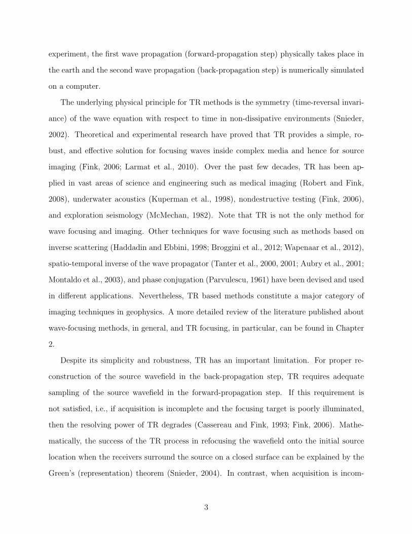
Figure 1.2 Illustration of the forward propagation (a), back projection with afull-aperture receiver array (b), and back projection with alimited-aperture receiver array (c) in a synthetic time-reversalexperiment. Back projection with a small-aperture receiver arraydistorts the focal pattern. Wave propagation is simulated in ahomogeneous acoustic medium. The white circles represent receivers. . . . . 4
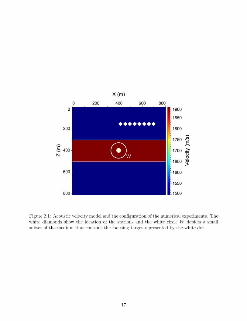
Figure 2.1 Acoustic velocity model and the configuration of the numericalexperiments. The white diamonds show the location of the stations andthe white circle W depicts a small subset of the medium that containsthe focusing target represented by the white dot. . . . . . . . . . . . . . . 17
Figure 2.2 Optimized signals computed using the BG method (left column)associated with receivers 1 to 8, and the corresponding time-reverseddata (right column). The weak reflected energy (green circle) in the TRtrace is amplified (red circle) in the optimized BG trace. . . . . . . . . . . 19
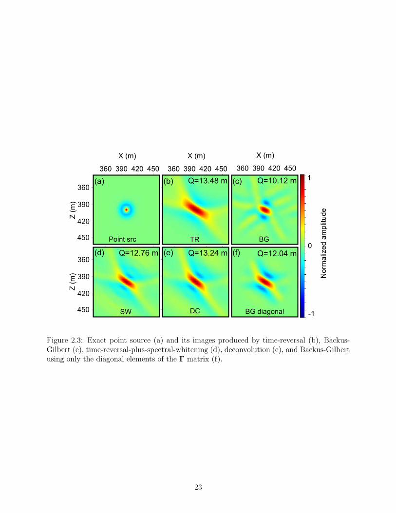
Figure 2.3 Exact point source (a) and its images produced by time-reversal (b),Backus-Gilbert (c), time-reversal-plus-spectral-whitening (d),deconvolution (e), and Backus-Gilbert using only the diagonal elementsof the Γ matrix (f). . . . . . . . . . . . . . . . . . . . . . . . . . . . . . . . 23
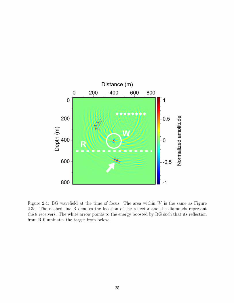
Figure 2.4 BG wavefield at the time of focus. The area within W is the same asFigure 2.3c. The dashed line R denotes the location of the reflector andthe diamonds represent the 8 receivers. The white arrow points to theenergy boosted by BG such that its reflection from R illuminates thetarget from below. . . . . . . . . . . . . . . . . . . . . . . . . . . . . . . . 25
ix
Figure 2.5 Comparison of BG and TR in imaging a dipole as an example of adistributed source with anisotropic radiation pattern. Snapshots of thewavefield associated with dipole sources with different orientations at thetime of source activation (left column) and their corresponding BGimages (middle column) and TR images (right column). . . . . . . . . . . . 28
Figure 2.6 Sensitivity test results. Images of a point source created with BG using(a) the true velocity model and optimization window of radius 60m(reference test), (b) smoothed velocity model, (c) perturbed velocity bydecreasing the velocity of the middle layer by 150m/s, (d) perturbedvelocity by decreasing the velocity of the middle layer by 200m/s, (e)altering the width of the middle layer by lowering its base boundary by60m, (f) altering the width of the middle layer by raising its baseboundary by 60m, (g) changing the width of the middle layer bylowering its top boundary by 60m, (h) changing the width of the middlelayer by raising its top boundary by 60m, (i) true velocity but increasingthe radius of the optimization window to 120m, (j) true velocity butincreasing the radius of the optimization window to 180m, (k) truevelocity model while contaminating the data with band-limited randomnoise with S/N = 2, (l) true velocity model while contaminating thedata with band-limited random noise with S/N = 1, (m) iterativeBackus-Gilbert in the time domain (BGT) after 2 iterations, (n) BGTafter 10 iterations, (o) BGT after 15 iterations, and (p) BGT after 30iterations. . . . . . . . . . . . . . . . . . . . . . . . . . . . . . . . . . . . 33
Figure 3.1 The elastic model and the configuration of the numerical experiment ofsection 3.5. The white diamonds show the location of the stations, thewhite circle W depicts a small subset of the medium that contains thefocusing target which is represented by the white dot. The bluebackground color represents vp = 3000m/s, vs = 2000m/s, andρ = 2000 kg/m3. The red background color represents vp = 3750m/s,vs = 2500m/s, and ρ = 3000 kg/m3. . . . . . . . . . . . . . . . . . . . . . 47
Figure 3.2 Vertical component of the optimal signals versus the timer-reversedvertical component of the data (left panel), and horizontal component ofthe optimal signals versus the time-reversed horizontal component of thedata (right panel). The weak reflection energies (green circles) areamplified in the optimized traces (red circles). . . . . . . . . . . . . . . . 50
Figure 3.3 Divergence (a) and curl (b) components of the source displacement fieldenclosed within W at the activation time of the source are comparedwith the P-wave (c) and S-wave (d) images of the source produced byBG, and with the P-wave (e) and S-wave (f) images of the sourceproduced by TR. . . . . . . . . . . . . . . . . . . . . . . . . . . . . . . . . 52
x

Figure 4.1 The elastic earth model and the source-receiver configuration for thenumerical sensitivity tests discussed in the text. The white diamondsshow the location of the receivers, the white circle W depicts a smallsubset of the medium (monitoring area) that contains the point sourcerepresented by the white dot. The blue background color representsvp = 3000m/s, vs = 2000m/s, and ρ = 2000 kg/m3. The red backgroundcolor represents vp = 3750m/s, vs = 2500m/s, and ρ = 3000 kg/m3. . . . 65
Figure 4.2 P-wave images of the point source associated with the source-receiverconfiguration depicted in Figure 4.1 showing (a) the true P-wave imageof the isotropic point source, (b) TR image using true velocity, (c) BGimage using true velocity and optimization window with radius 90m, (d)BG image where BG is applied partially such that the interplay betweenreceiver components among different stations is ignored, (e) BG imageusing a perturbed model where the density and velocities of the middlelayer are decreased by 10%, (f) BG image using a perturbed modelwhere the density and velocities of the middle layer are decreased by 5%,(g) BG image using a perturbed model where the density and velocitiesof the middle layer are increased by 5%, (h) BG image using a perturbedmodel by smoothing the true velocity with a Gaussian filter, (i) BGimage using a perturbed model where the width of the middle layer isaltered by lowering its base interface by 60m, and (j) by raising its baseinterface by 60m, and (k) by lowering its top interface by 60m, and (l)by raising its top interface by 60m, (m) BG image using the truevelocity and optimization window W with radius 120m, (n) BG imageusing the true velocity and optimization window W with radius 180m,(o) BG image using the true velocity and data contaminated by noisewith S/N = 2, and (o) BG image using the true velocity and datacontaminated by noise with S/N = 1. All images are obtained bycomputing the divergence of the injected wavefield at the time of focus. . . 66
Figure 4.3 Resolution test for the linear receiver geometry. Panel (a) shows theconfiguration of the receivers (the diamonds) and the trial sourcelocations (9 white dots). Panel (b) contains 9 images which are impulseresponses for 9 BG source-imaging experiments, imaging point sources atthe white dots shown in panel (a). Panel (c) contains 9 images which areimpulse responses for 9 TR source-imaging experiments, imaging pointsources at the white dots shown in panel (a). . . . . . . . . . . . . . . . . . 72
xi
Figure 4.4 Resolution test for the scattered receiver geometry. Panel (a) shows theconfiguration of the receivers (the diamonds) and the trial sourcelocations (9 white dots). Panel (b) contains 9 images which are impulseresponses for 9 BG source-imaging experiments, imaging point sources atthe white dots shown in panel (a). Panel (c) contains 9 images which areimpulse responses for 9 TR source-imaging experiments, imaging pointsources at the white dots shown in panel (a). . . . . . . . . . . . . . . . . . 73
Figure 4.5 Imaging of a double-couple source with different orientations. Theorientation of the source is specified by the angle θ measured relative tohorizontal. The receiver geometry is the same as that shown in Figure4.3a and the source is at location 4. Top panel: The first row in the toppanel shows the divergence of the BG-optimized wavefield at the time offocus (the P-wave image) for different orientations of the double-couplesource. The second row in the top panel depicts the true P-wave imageof the double-couple source with different orientations of the source.Bottom panel: The first row in the bottom panel shows the curl of theBG-optimized wavefield at the time of focus (the S-wave image) fordifferent orientations of the double-couple source. The second row in thebottom panel depicts the true S-wave image of the double-couple sourcewith different orientations of the source. . . . . . . . . . . . . . . . . . . . 75
Figure 5.1 Depths are most highly correlated in the strike direction of the slab.Point D is located somewhere between points A and B in the slab strikedirection. In this configuration, although D’ is closer to C’, the depth atD’ is more similar to the depth at A’ and B’ than it is to the depth atC’. γ denotes the strike angle defined as the azimuth of the strikemeasured relative to geographic north N . Dip is perpendicular to thestrike direction. δ denotes the dip angle measured relative to horizontal. . 84
Figure 5.2 Scattered depth estimates and uncertainties. Scattered estimates ofsubducting slab depths (a) and estimates of uncertainties (b) specified asthe standard deviation of the errors associated with depth data. Thesolid black line represents the west coast of South America. The datapoints depicted here have been gridded according to the proceduredescribed in the text and consist of 2675 earthquake source locations,344 measurements from active-source seismic surveys (data points alonglinear tracks perpendicular to the coastline), and 2057 measurementsfrom bathymetry surveys (data forming a stripe, parallel to thecoastline). . . . . . . . . . . . . . . . . . . . . . . . . . . . . . . . . . . . 88
xii

Figure 5.3 Interpolation of strikes. Scattered strike data (a) are interpolated on thecurved surface of the Earth to construct a uniformly sampled strike field(b). The strike field shown in (c) is the result of the 40th iteration ofinterpolating the scattered strikes guided along the slab dip direction.White ellipses in (b) represent the tensor field G that was used to guidethe interpolation on the curved surface of the Earth. These ellipses areelongated as they account for the curvature of the Earth’s surface whenprojected onto an equi-rectangular longitude-latitude coordinate system.The white ellipses in (c) are elongated in the slab dip direction and areused to guide the interpolation of strikes in the dip direction. . . . . . . . 90
Figure 5.4 Two interpolations of slab depths. A strike-ignorant interpolation (a) ofslab depths on the Earth’s surface, in which the metric tensor field usedto guide the interpolation of depths accounts for only the differencebetween Euclidean and geodesic distance and a strike-guidedinterpolation (b) in which the metric tensor field also accounts forestimated strike directions. Ellipses represent the metric tensor fields. . . 92
Figure 5.5 Cross-validation results. Cross-validation root mean square (rms)normalized error computed for the strike-guided interpolant as afunction of η. The normalization involves dividing the cross-validationerror at each data point by the estimate of the uncertainty (standarddeviation) associated with that point. The rms error curve has aminimum of 2.82 at η = 92 denoted by the cross. The area within theellipse is magnified in the subfigure to show the location of theminimum. The value of the rms normalized error at η = 0 correspondingto the strike-ignorant interpolation is 6.34. . . . . . . . . . . . . . . . . . 94
Figure 5.6 An approximate smooth model σ(x) of the standard deviation of theerror associated with depth data. This model is used to design aspatially varying smoothing function. . . . . . . . . . . . . . . . . . . . . . 98
Figure 5.7 A cross section (a) showing the profiles of three different slab models.The slab model obtained by tensor-guided interpolation (b) is comparedwith the model obtained by tensor-guided fitting (c) and the same modelfrom Slab1.0 (d) produced by Hayes et al. Line segment AB shows thegeographical location of the vertical cross section shown in (a). The graycrosses in (a) are the orthogonal projection of all data points (the pointsshown in white in (b), (c), and (d)) that lie within a rectangular windowof width 100 km centered on the vertical plane of section AB. The graydots in (b), (c), and (d) denote the location of scattered data points. . . 101
Figure 5.8 Histogram of the standardized fitting errors rk for the optimal smoothingfunction computed using smoothing parameter s = 0.56. . . . . . . . . . 104
xiii

ACKNOWLEDGMENTS
The past four years of my life at Colorado School of Mines have been a wonderful in-
tellectual journey. As a research assistant at the Center for Wave Phenomena (CWP), my
day-to-day responsibilities consisted of working with, learning from, and interacting with
world-class scientists. I simply had the best job in the world! I am grateful to Dave Hale for
giving me this opportunity by accepting me to CWP. Dave, thank you for setting such high
standards for science, research, and teaching for us. I have learned from you in many direct
and indirect ways.
I consider myself extremely privileged because I was able to attend classes taught by
Ilya Tsvankin, and Paul Sava. Ilya and Paul, I cannot say how much I enjoyed learning
geophysics from you and how deeply I appreciate your commitment to education.
Ken Larner’s vision for excellence in geophysical research has been a perpetual guide
for students and faculty in CWP. Dear Ken, thank you for sharing your superb taste in
communicating scientific ideas with the rest of us.
Even the best research ideas, if not communicated effectively, are futile. Developing
writing skills and cultivating presentation abilities have been a central aspect of education
at CWP. I am greatly thankful to Diane Witters for her instructions on writing, presentation,
and general communication skills. Diane, you have a unique way of helping students with
their individual needs. Because of your help, I have come a long way in technical writing
and feel much more confident about it. I am also thankful for your friendship. You are a
blessing to CWP.
The perfect learning environment in the Geophysics Department is the result of col-
laboration of many talented and devoted individuals. The department always felt like a
second home because people like Pamela Kraus, Shingo Ishida, Michelle Szobody, and Dawn
Umpleby do more than just their jobs and keep going out of their way to help students with
xiv

all their educational needs. The leading role and vision of Terry Young in establishing the
value system in the department cannot be ignored. Dear Terry, thank you for creating an
ideal learning environment.
I must also thank my friends and colleagues without whom I would not have been able
to succeed at Mines. Simon Luo, Nishant Kamath, Steve Smith, Stefan Compton, Luming
Liang, Alison Knaak, Chinaemerem Kanu, Oscar Jarillo, Esteban Diaz, Yuting Duan, and
Satyan Singh, I am truly grateful for your friendship and for the valuable things I have
learned from you. I hope our friendship will last and I can work with you again at some
point in the future.
My two summer internships with Shell provided me with ample opportunities to grow as
a geophysicist. I am especially thankful to Jan Douma and Jon Sheiman for those opportu-
nities. Jan, the great things that I have learned from you are not limited to geophysics. I
enjoyed our brain-storming sessions over coffee. Jon, your vast knowledge and experience,
your passion for figuring things out, and your humility make you a scientist that I deeply re-
spect and look up to. Thank you for the invaluable insights that you brought to my research.
I look forward to learning more from you.
In my life, I have been blessed with continual and unconditional love from my parents.
Mother and Father, thank you for supporting me all my days. Thank you for giving me
hope.
It is hard to find proper words to express my gratitude towards my advisor Roel Snieder.
Before coming to Mines, I had searched around the world for a perfect teacher, a wise and
selfless person with a heart full of love and passion for education. When I came to know
Roel, my search was over. Dear Roel, you have been the good shepherd. You took my hand
and helped me overcome my fears. I have heard words of wisdom from you. I have seen an
example of a good life in you. I could not have asked for more! Your flawless advising style
reminds me of this piece from the Tao Te Ching:
xv

The best leaders are those the people hardly know exist.
The next best is a leader who is loved and praised.
Next comes the one who is feared.
The worst one is the leader that is despised.
If you don’t trust the people,
they will become untrustworthy.
The best leaders value their words, and use them sparingly.
When she has accomplished her task,
the people say, ”Amazing:
we did it, all by ourselves!”1
1Translated by J. H. McDonald
xvi

Your face, O Lord, I shall seek.
xvii

CHAPTER 1
INTRODUCTION
Earthquake source characterization continues to be an important area of research in seis-
mology. Characterizing seismic sources helps geophysicists with understanding the physics
of earthquakes and faulting processes (Shearer, 2009; Baig and Urbancic, 2010). With the
advent of hydraulic fracturing in unconventional hydrocarbon resources and with the need
for monitoring the affected volume of rock in tight reservoirs, mapping and characterizing the
micro-earthquakes that occur during the fracturing process has become even more important
(Maxwell and Urbancic, 2001; Shapiro, 2008; Eisner et al., 2010).
Conventional seismic methods for source characterization invert kinematic information in
seismic data (e.g., P- and S-wave arrival times) for source parameters such as time, location,
and moment tensor (Stein and Wysession, 2009). More advanced techniques use the full
waveform data for the same purpose. These inversion-based techniques minimize the full
waveform differences between the observed data and simulated seismograms (Kim et al.,
2011; Song and Toksoz, 2011)
Time-reversal (TR) methods take an alternative approach to source characterization
which is to directly image the source by back projecting seismic data into the medium
(McMechan et al., 1985; Larmat et al., 2006; Kawakatsu and Montagner, 2008; Lu et al.,
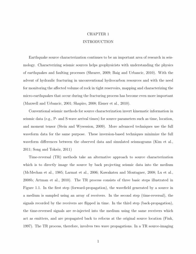
2008b; Artman et al., 2010). The TR process consists of three basic steps illustrated in
Figure 1.1. In the first step (forward-propagation), the wavefield generated by a source in
a medium is sampled using an array of receivers. In the second step (time-reversal), the
signals recorded by the receivers are flipped in time. In the third step (back-propagation),
the time-reversed signals are re-injected into the medium using the same receivers which
act as emitters, and are propagated back to refocus at the original source location (Fink,
1997). The TR process, therefore, involves two wave propagations. In a TR source-imaging
1

η
η
(a)
(b)
(a)
(b)
Figure 1.1: Time-reversal experiment. (a) Forward-propagation (first step): waves excitedby a source travel through the complex medium and are recorded at stations marked ascircles. (b) Back-propagation (second and third steps): the recorded signals are reversedin time and rebroadcast into the medium at the corresponding stations. The waves thenpropagate through the medium and converge on the original source location (after Lu et al.(2008a)).
2
experiment, the first wave propagation (forward-propagation step) physically takes place in
the earth and the second wave propagation (back-propagation step) is numerically simulated
on a computer.
The underlying physical principle for TR methods is the symmetry (time-reversal invari-
ance) of the wave equation with respect to time in non-dissipative environments (Snieder,
2002). Theoretical and experimental research have proved that TR provides a simple, ro-
bust, and effective solution for focusing waves inside complex media and hence for source
imaging (Fink, 2006; Larmat et al., 2010). Over the past few decades, TR has been ap-
plied in vast areas of science and engineering such as medical imaging (Robert and Fink,
2008), underwater acoustics (Kuperman et al., 1998), nondestructive testing (Fink, 2006),
and exploration seismology (McMechan, 1982). Note that TR is not the only method for
wave focusing and imaging. Other techniques for wave focusing such as methods based on
inverse scattering (Haddadin and Ebbini, 1998; Broggini et al., 2012; Wapenaar et al., 2012),
spatio-temporal inverse of the wave propagator (Tanter et al., 2000, 2001; Aubry et al., 2001;
Montaldo et al., 2003), and phase conjugation (Parvulescu, 1961) have been devised and used
in different applications. Nevertheless, TR based methods constitute a major category of
imaging techniques in geophysics. A more detailed review of the literature published about
wave-focusing methods, in general, and TR focusing, in particular, can be found in Chapter
2.
Despite its simplicity and robustness, TR has an important limitation. For proper re-
construction of the source wavefield in the back-propagation step, TR requires adequate
sampling of the source wavefield in the forward-propagation step. If this requirement is
not satisfied, i.e., if acquisition is incomplete and the focusing target is poorly illuminated,
then the resolving power of TR degrades (Cassereau and Fink, 1993; Fink, 2006). Mathe-
matically, the success of the TR process in refocusing the wavefield onto the initial source
location when the receivers surround the source on a closed surface can be explained by the
Green’s (representation) theorem (Snieder, 2004). In contrast, when acquisition is incom-
3

FORWARD PROPAGATION
BACK PROPAGATIONFULL APERTURE
BACK PROPAGATIONLIMITED APERTURE
1
2
3
4
1
2
3
1
2
3
4 4
(a) (b) (c)
Tim
e
Figure 1.2: Illustration of the forward propagation (a), back projection with a full-aperturereceiver array (b), and back projection with a limited-aperture receiver array (c) in a syn-thetic time-reversal experiment. Back projection with a small-aperture receiver array distortsthe focal pattern. Wave propagation is simulated in a homogeneous acoustic medium. Thewhite circles represent receivers.
4
plete, the prerequisites of the Green’s theorem are not satisfied and it breaks, and so does
the TR process. Figure 1.2 demonstrates this problem with a numerical simulation of a TR
experiment. Figure 1.2a shows the first step of the TR process where the energy generated
by a point source propagates through a homogeneous medium and is adequately sampled
by a full-aperture array of receivers (the white circles) surrounding the source. Figure 1.2b
demonstrates the back-propagation step where, after time reversing, the signals recorded in
the first step are back projected into the medium and ultimately focus on a finite-sized spot
at the original source location and provide a nearly perfect image of the point source. The
size of focal spot in this figure is finite because in a diffraction-limited imaging process such
as TR, the minimum size of the focal spot is bounded by the diffraction limit and is approx-
imately equal to half the dominant wavelength of the propagating waves (Born and Wolf,
1999). The focal spot shown in Figure 1.2b (part 4) is effectively the point spread function of
the TR experiment. However, if the receiver array in this example is replaced with a limited
aperture array, then, as shown in Figure 1.2c, the back-propagation step cannot recover a
well-resolved and focused image of the source. The distortion of the point spread function
observed in Figure 1.2c (part 4) is a consequence of incomplete acquisition.
The requirement for complete acquisition poses a significant practical limitation on TR
imaging. This is because in most applications, such as in earthquake source imaging or
microseismic monitoring, receiver arrays are sparse and clustered in space, meaning that
adequate sampling of the source wavefield is not possible in practice. This raises the question
of whether TR is an optimal process for imaging the source in most such applications.
In this thesis, I study the TR process with the goal of optimizing its resolution in sit-
uations where the receiver array geometry does not allow adequate sampling of the source
wavefield. The main focus of the research is on improving the second step of the TR process,
where the key question is how the recorded data can be processed alternatively (instead of
time-reversing) to achieve optimal resolution in a TR experiment with incomplete acquisi-
tion. To this end, I propose a new approach where source imaging is posed as an optimization
5
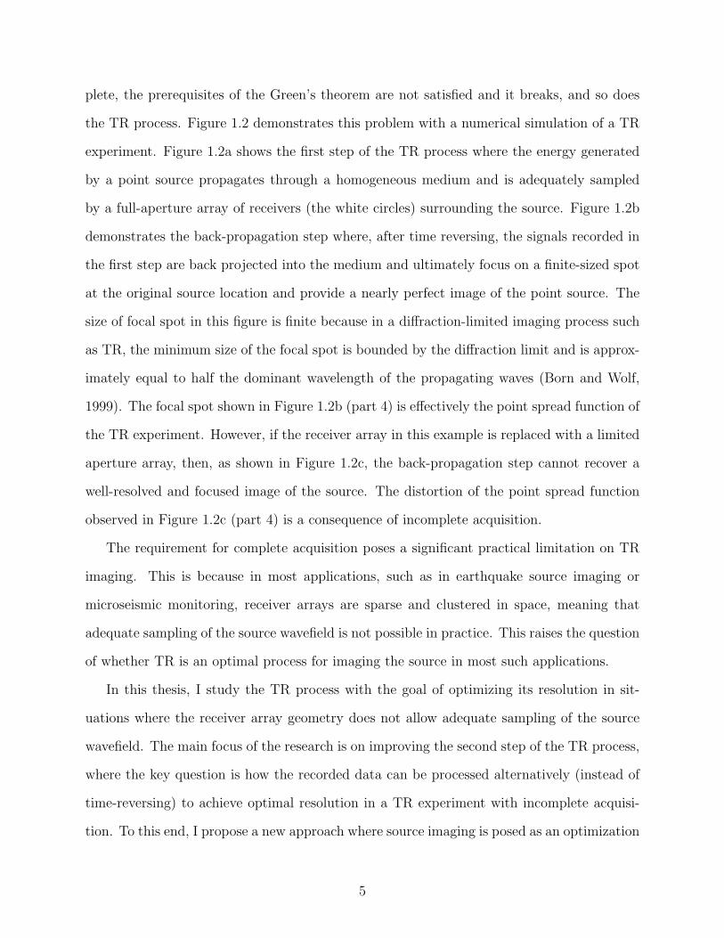
problem and is solved using a technique based on the method of Backus and Gilbert in geo-
physical inverse theory. The method of Backus and Gilbert (Backus and Gilbert, 1967,
1968, 1970), provides a general mathematical treatment of resolution in continuous or dis-
crete and underdetermined linear inverse problems. The method obtains a unique solution
to an underdetermined linear problem by constructing an optimal resolution matrix that
most closely resembles the identity matrix (Aki and Richards, 1980; Snieder and Trampert,
1999; Tarantola, 2005; Menke, 2012). Because seismic source imaging is essentially an un-
derdetermined linear inverse problem, it can be aptly studied in the framework of Backus
and Gilbert theory.
The proposed approach, named Backus-Gilbert (BG) source imaging, provides an im-
proved resolution for source imaging compared to the time-reversal approach. The method
can be used for imaging extended source as well as point sources and, moreover, it is capable
of retrieving the mechanism of the source. The BG method does not require a-priori infor-
mation about the location of the source or its time function. The only requirements of the
BG method are the data recorded by the receivers, accurate knowledge of the propagation
medium, and an estimate of the source location.
1.1 Thesis outline
The next four chapters in this dissertation are presented as individual research papers.
Chapters 2-4 share the common theme of optimal wave focusing and Backus-Gilbert source
imaging. Chapter 5 is devoted to the problem of modeling the geometry of the subducting
slab interface in South America using a tensor-guided data-fitting method. The primary
input data used by this data-fitting method consist of estimates of the depth of the slab
and the uncertainty in such estimates. These depth estimates are inferred from the location
of the source of the earthquakes associated with the subduction process in South America.
The secondary input data consist of estimates of the strike angle of the slab which are
inferred from the focal mechanisms of subduction-related earthquakes. The proposed data-
fitting method uses the secondary data to guide the interpolation of the primary data. The
6
depth and focal mechanism of the earthquakes are normally obtained by conventional source
inversion techniques. The ability of the BG method in retrieving source parameters such as
location and source mechanism and its potential for delineating the spatial extension of the
source could be advantageous for constructing a more accurate slab model. An overview of
Chapters 2-5 and the way they are related is given in the following paragraphs..
In Chapter 2, I develop the Backus-Gilbert (BG) method for source imaging in acoustic
media. I first introduce the BG optimization approach to the problem of focusing acoustic
waves at a desired time and location inside a medium with known properties. Knowing how
to focus waves is important because it provides a basis for the BG source imaging algorithm.
Using source-receiver reciprocity of the Green function, I next show that BG focusing can
be adapted and applied for imaging an acoustic point source originating from an unknown
location and time. The BG method is also applicable for imaging spatio-temporally extended
sources. This, as shown in Appendix A, is a consequence of the linearity of the source
imaging problem and the superposition principle. Throughout Chapter 2, the BG method
is tested using numerically simulated sources in a synthetic layered acoustic medium. The
resulting BG images of the source in these tests are analyzed and compared with the same
images produced by the TR method. At the end of the chapter, I discuss the sensitivity
of the BG method to noise in data, inaccuracies in the medium properties, and uncertainty
in the estimate of source location. The BG method in Chapters 2 and 3 is formulated
in the frequency domain. This frequency-domain formulation requires computing the Green
function for each receiver location. This requirement can make of the BG method impractical
for surface microseismic surveys which could involve thousands of receivers. To tackle this
problem, I present a time-domain formulation of the BG method in Appendix B. This
time-domain formulation does not depend on the Green functions for the receiver locations.
In Chapter 3, I generalize the theory of the BG method for elastic waves. Earthquake
sources occur in the solid Earth and generate elastic waves. Therefore, the BG method
for source imaging must be extended for application in elastic media. I first derive the
7

BG method for imaging an elastic point source with an unknown moment tensor in an
elastic medium with known properties. This derivation involves the assumption that particle
displacements in the near-source region are proportional to the source equivalent force. I
justify this assumption in Appendix C. Later, in Appendix D, I show that the method is
equally applicable for imaging an extended source. Although the derivation of the elastic
BG method is theoretically more involved, the method ultimately ends up having the same
mathematical form as in the acoustic case. To solve the elastic BG optimization problem,
one only requires the data recorded in the field, an estimate of the source location, and
knowledge of the elastic medium. I next test the elastic BG method using a numerical
experiment for imaging a double-couple source with a limited-aperture receiver array. This
test demonstrates that the BG method can produce significantly better resolved P- and S-
wave images of the double-couple source compared to the same images produced by TR.
For this improvement, the BG method takes advantage of the reflection energy in data to
compensate for limited aperture of the receiver array.
Chapeter 4 is devoted to sensitivity tests and analysis of the solution that the BG
method provides for the source imaging problem. Source imaging can be expressed as an
underdetermined linear inverse problem with infinitely many potential solutions that can
explain the data. I first analyze the BG method theoretically and show that the solution
it provides is equivalent to the minimum L2-norm solution to the underdetermined source-
imaging problem. Next, using numerical simulations, I investigate the sensitivity of the
elastic BG method to errors in the earth model and noise in data. I also examine how the
BG solution is affected by the size of the monitoring area. Finally, I explore the potentials
and limitations of the method for studying the resolution of the BG method in an experiment
with a given configuration.
In Chapter 5, I present a novel gridding method for interpolating scattered data points
representing earthquake locations. Earthquakes provide estimates of depths of subducting
slabs, but only at scattered locations. These depth estimates can be interpolated to construct
8

a model for the subducting slab as a uniform function of space. In addition to estimates of
depths from earthquake locations, focal mechanisms of the subduction-related earthquakes
also provide estimates of the strikes of the subducting slab. I use these spatially sparse strike
samples to infer a model for spatial correlation that guides a blended neighbor interpolation
of slab depths. A brief review of the blended-neighbor interpolation is provided in Appendix
E. The interpolation method is then modified to account for the uncertainties associated
with the depth estimates. I illustrate the gridding (data fitting) method using data from the
South American subduction zone. In Appendix F, I present a weighted averaging scheme
to compute a minimum-variance average of measurements (here depth samples) with known
variances.
The data requirements of the proposed fitting method are estimates of slab depth, un-
certainties in depth measurements, and estimates of slab strikes. All this information is
obtained by characterizing subduction-related earthquakes. Using BG to image earthquake
sources could provide more accurate information about them (e.g., location, mechanism, spa-
tial extension, and the rupture process) compared to other source characterization methods,
especially for earthquakes in poorly instrumented areas. Therefore, the data fitting method
proposed in Chapter 5 may benefit from the BG method introduced in the previous chapters.
Chapter 6 is a summary containing general conclusions and final remarks about this
thesis and some recommendations for future research.
Chapters 2-5 have been or soon will be published in, peer-reviewed journals:
• Bazargani, F, R. Snieder, and Jon Sheiman, 2014, Optimal wave focusing in acoustic
media: Geophysical Journal International (to be submitted).
• Bazargani, F and R. Snieder, 2014, Optimal wave focusing in elastic media: Geo-
physical Journal International (to be submitted).
• Bazargani, F., D, Hale, and G. P. Hayes, 2013, Tensorguided fitting of subducting
slab depths: Bulletin of the Seismological Society of America, 103, 2657-2669.
9

During my PhD study, I also contributed to the following conference publications:
• Bazargani, F and R. Snieder, 2014, Optimal wave focusing in elastic media: SEG,
Expanded Abstracts (accepted).
• Bazargani, F and R. Snieder, 2013, Optimal wave focusing for imaging and micro-
seismic event location: SEG, Expanded Abstracts 2013: pp. 4595-4600.
• Behura, J, F. Bazargani, and F. Forghani, 2013, Improving microseismic imaging:
role of acquisition, velocity model, and imaging condition: SEG, Expanded Abstracts
2013: pp. 2119-2123.
10

CHAPTER 2
OPTIMAL WAVE FOCUSING IN ACOUSTIC MEDIA
A paper to be submitted to the Geophysical Journal International
Farhad Bazargani1, Roel Snieder1, and Jon Sheiman2
2.1 Abstract
Focusing waves inside a medium has applications in various science and engineering fields,
such as in medicine, nondestructive evaluation, ocean acoustics, and geophysics. The goal
in wave focusing is to concentrate the wave energy at a specific time and location inside a
medium. Various techniques have been devised and used to achieve this goal. Time-reversal
is a method that is routinely used to focus acoustic and seismic waves. One important
geophysical application of time-reversal focusing is in seismic source imaging. However, the
method is not optimal for source imaging when acquisition is incomplete. Inspired by the
Backus and Gilbert method in inverse theory, we propose a technique wherein wave focusing
is cast as an optimization problem. Using numerical experiments, we demonstrate that our
new technique mitigates the adverse effects that incomplete acquisition has on time-reversal
focusing and source imaging. The only requirements of the method are knowledge of the
medium and an estimate of the source location.
2.2 Introduction
The objective in wave focusing is to determine the waveforms that, when transmitted
through a medium, create a wavefield that concentrates at a specific time and location.
Wave focusing is conceptually related to the problem of imaging, and hence finds important
applications in areas such as seismology and exploration geophysics.
1Center for Wave Phenomena, Colorado School of Mines, Golden, Colorado 80401, USA2Shell International Exploration and Production, Houston, Texas 77079, USA
11

Several methods for focusing have been devised, including those based on inverse scat-
tering (Haddadin and Ebbini, 1998; Broggini et al., 2012; Wapenaar et al., 2012), phase
conjugation (Parvulescu, 1961), and time-reversal (Fink, 1997). Time-reversal (TR) is a
well-established focusing technique that is robust and effective in heterogeneous media. The
method relies on the time-reversal invariance of the wave operator and spatial reciprocity
(Snieder, 2002).
A time-reversal mirror is an array of transducers (receivers), each capable of recording,
time-reversing (last-in first-out), and retransmitting signals into the medium. The TR pro-
cess consists of three basic steps. In the first step, the wavefield generated by a source in
the medium is recorded using a TR mirror. In the second step, the recorded waveforms are
time-reversed. Finally, in the third step, the time-reversed signals are re-injected into the
medium, and propagated back to refocus at the original source location. In a dissipative
medium, time-reversal invariance is not satisfied (Snieder, 2004; Zhu, 2014). Nevertheless,
spatial reciprocity alone explains the robustness and efficiency of the TR process in many
applications involving dissipative media (Fink, 2006).
TR focusing has been implemented in a variety of scenarios. It is applicable to both
physical and numerical (modeling) back-propagation experiments. In both, one deals with
propagation of a time-reversed field, but the propagation is real in a physical problem and
simulated in a numerical problem (Fink, 2006). Applications involving physical TR include
medical imaging (Robert and Fink, 2008), lithotripsy, underwater acoustics, and nondestruc-
tive testing (Fink, 1997; Edelmann et al., 2002; Robert and Fink, 2008; Fink and Tanter,
2010; Larmat et al., 2010). Numerical back-propagation methods, also known as time-
reversal modeling techniques, are applied in key areas of geophysics on both global and
exploration scales. In global seismology, TR modeling techniques are used for seismic source
imaging, for monitoring nuclear explosions, and in environmental applications of geophysics
(McMechan, 1982; McMechan et al., 1985; Lu et al., 2008a; Larmat et al., 2006; Lokmer
et al., 2009; Larmat et al., 2010). In exploration seismology, TR modeling is used in mi-
12
croseismic event location and reservoir monitoring (Gajewski and Tessmer, 2005; Lu et al.,
2008a; Shapiro, 2008; Steiner et al., 2008; Larmat et al., 2009; Xuan and Sava, 2010), in
salt-flank imaging and redatuming seismic data (Lu et al., 2008a), and in reversed time
migration (McMechan, 1983; Berkhout, 1997; Schuster et al., 2002).
Despite these broad applications, the TR process has important theoretical and practical
limitations. In theory, for a broadband pulse emitted by an ideal point source, the returning
field refocuses on a spot with dimensions on the order of the smallest wavelength (Abbe
diffraction limit). This is because evanescent waves containing source details smaller than
the involved wavelengths cannot be sensed in the far-field. The loss of this information
causes the resolution of the process to be bounded by the diffraction limit (Fink, 1997).
Moreover, in practice, the wavefield is sampled at spatially sparse and limited locations.
Also, it is not practical to surround the source with a full-aperture TR mirror, so a finite-
aperture TR mirror is used instead. This incomplete acquisition results in a distortion
in the shape of the point-spread function (the impulse response) of the TR experiment
(Cassereau and Fink, 1993; Fink, 2006; Artman et al., 2010). Another problem is that in
real applications of TR-focusing, the media are dissipative and time-reversal invariance of the
wave equation does not hold valid in dissipative media. However, as shown by Fink (2006),
even in a dissipative medium, the TR process always maximizes the output amplitude at the
focal time although it does not impose any constraints on the field around the focus. For
example, side lobes can be observed around the source.
Several studies have been devoted to the limitations of TR modeling and offer techniques
to mitigate their effects. Zhu (2014) proposes a TR modeling approach that compensates for
attenuation and dispersion effects due to wave propagation in dissipative media. Tanter et al.
(2000, 2001), Aubry et al. (2001), and Montaldo et al. (2003) present the spatio-temporal
inverse-filter method, a focusing technique based on the inverse of the wave propagator
between a source and elements in a TR mirror. For a lossless medium, the inverse filter
method yields the same result as that of the TR method, but in the presence of attenuation,
13

the spatio-temporal inverse filter methods are more effective than is the TR method.
Research on the connection between medium complexity and the size of the focal spot
has shown a direct relationship between the complexity of the medium and the resolution in
TR focusing; the more complicated the medium between the source and the TR mirror, the
sharper the focus (Blomgren et al., 2002; Fink, 2008; Vellekoop et al., 2010). This is because
a finite-aperture TR mirror acts as an antenna that uses complex environments to appear
wider than it actually is, resulting in a focusing capability that is less dependent on the
aperture of the TR mirror. In media consisting of a random distribution of sub-wavelength
scatterers, a time-reversed wavefield can interact with the random medium to regenerate not
only the propagating but also evanescent waves required to refocus below the diffraction limit
(super-resolution). Schuster et al. (2012) demonstrate a method that uses evanescent waves
generated by scatterers in the near-field region of seismic sources to achieve super-resolution.
As discussed above, TR focusing methods are not optimal because of limitations such
as imperfect acquisition, attenuation, and the diffraction limit. We propose an alternative
approach to wave focusing wherein the problem is cast as an optimization problem. The
motivation for this research is to improve upon the existing TR modeling techniques in
dealing with the limitations caused by incomplete acquisition.
The organization of the paper is as follows: We first lay out the theoretical foundation
of our new approach to wave focusing and show how to design waveforms that optimally
focus at a desired known location and time inside a medium. Next we discuss how the
new method, named Backus-Gilbert focusing (BG), is connected to some other focusing
techniques like time-reversal and show that such other techniques are special cases of the
more general solution to wave focusing that our approach provides. In the next step, we show
how, with a modicum of modification and reinterpretation, the BG theory can be adapted
for application in source-imaging problems. We start by adapting the BG theory for imaging
a single point source, and in Appendix A we generalize the theory for an arbitrary spatio-
temporally distributed source without knowing the properties of the source. We then show
14

two simple but representative numerical examples that demonstrate the application of the
BG method in imaging of a point source and then a dipole source. Next, we discuss various
aspects of the method and elaborate further on some explicit and implicit assumptions that
are used in the construction and parameterisation of the new method and discuss their
significance. Finally, in Appendix B, we show an alternative time-domain formulation of the
idea that underlies the BG method.
2.3 Focusing as an optimization problem
We will use the following notational conventions to facilitate the formulation of the new
ideas presented in this chapter.
2.3.1 Notation
1. All superscripts are associated with the receivers and take any integer value between 1
and N .
2. We use Einstein’s notation for repeated indices: whenever an index (a superscript) is
repeated, summation over that index is implied.
3. Fourier transforms follow the convention
f(x, ω) =
∫f(x, t) eiωt dt.
4. A Green function G(xi, t; ξ, 0) denotes the value the scalar pressure field measured at
x = xi and time t, where the pressure field is generated by an impulsive source at x = ξ and
t = 0.
5. As a superscript, the asterisk ∗ denotes complex conjugation, and when the symbol is
used inline, it represents the time convolution of two functions.
2.3.2 Formulation
Consider an acoustic medium with known velocity and N receiver stations at distinct
locations xi wherein each station records signals for T seconds for times 0 < t < T . Suppose
15

that at some time τ ∈ [0, T ] an impulsive point source at location x = ξ goes off and
generates an acoustic wavefield that is eventually sampled by the N receivers as di(t).
In the time-reversal method, we focus acoustic energy at x = ξ and at t = T − τ by
rebroadcasting the shifted time-reversed signals di(T − t) at each station. However, because
of the incomplete acquisition geometry of the receivers, the focus created by this TR process
is suboptimal. Our objective is to design signals that, upon transmission, focus optimally
at the target location ξ and at the time T − τ . To achieve the best spatio-temporal focus,
each station must work in concert with the others by injecting a signal that is tailored in
amplitude and in shape according to the medium properties, location of the focusing target,
and the geometry of the stations. If we denote the signal injected by the station at xi as
ai(t), then the superposed injected acoustic scalar wavefield at an arbitrary location x inside
the medium is
φ(x, t) = ai(t) ∗G(x, t; xi, 0). (2.1)
If the medium is known, these Green functions G(x, t; xi, 0) can be computed. Note the use
of Einstein notation, implying summation over repeated indices, in equation 2.1.
Convolution in the time domain corresponds to multiplication in the frequency domain.
Therefore, considering the problem in the frequency domain, each frequency component of
the wavefield φ(x, t) in equation 2.1 can be expressed as a weighted sum of the corresponding
frequency component G(x; xi, ω) of the Green functions, i.e.,
φ(x, ω) = ai(ω)G(x; xi, ω), (2.2)
where the weights ai(ω) are the Fourier components of the signal injected by the station at
xi.
The problem can now be restated as how to optimally determine the unknown weights
ai(ω) in equation 2.2 so that the superposed field φ in the time domain focuses at a desired
focal location ξ and at a desired focal time T−τ . Put another way, the goal is to have φ(x, t)
16
Z (m
)
X (m)
Velo
city
(m/s
)
W
Figure 2.1: Acoustic velocity model and the configuration of the numerical experiments. Thewhite diamonds show the location of the stations and the white circle W depicts a smallsubset of the medium that contains the focusing target represented by the white dot.
17

as close as possible to δ(x − ξ) δ(t − T + τ), where δ denotes the Dirac delta function. In
the frequency domain, this goal can be achieved if we let each frequency component φ(x, ω)
approach eiω(T−τ)δ(x− ξ) by minimizing an objective function defined as
J =
∫W
|φ(x, ω)− eiω(T−τ)δ(x− ξ)|2dx, (2.3)
where W denotes a subset of the medium that contains the target location (Figure 2.1).
Inserting equation 2.2 in objective function 2.3 and minimizing with respect to ai(ω)
results in a linear system of equations of the form
Γ(ω)a(ω) = eiω(T−τ)g∗(ω), (2.4)
where Γ is an N ×N Gram matrix (Parker, 1994) defined by its elements as
Γij(ω) =
∫W
G(x; xi, ω)G∗(x; xj, ω) dx, (2.5)
a(ω) is an N × 1 vector that is the unknown of the equation, and g is an N × 1 vector with
elements
gi(ω) = G(ξ; xi, ω). (2.6)
The linear system in equation 2.4 can be solved for the vector a(ω) for each frequency
separately. These a(ω) vectors constitute the Fourier coefficients for the signals that the
stations must inject to obtain an optimal focus at location ξ and at time T − τ .
The condition that is implied by minimizing the objective function 2.3 is known as the
deltaness criterion in the context of the method of Backus and Gilbert in inverse theory
(Backus and Gilbert, 1968). Useful descriptions of this method can be found in Aki and
Richards (1980), Tarantola (2005), Menke (2012), and Aster et al. (2013). Henceforth, we
refer to the method described above for designing optimal signals for wave focusing as the
Backus-Gilbert (BG) method.
18

BG TRN
orm
aliz
ed a
mpl
itude
1
1
1
1
1
1
1
1
-1
-1
-1
-1
-1
-1
-1
-1
0
0
0
0
0
0
0
0
0 0.2 0.4 0 0.2 0.4
Time (s) Time (s)
a1(t)
a2(t)
a3(t)
a4(t)
a5(t)
a6(t)
a7(t)
a8(t)
d2(0.4� t)
d3(0.4� t)
d4(0.4� t)
d5(0.4� t)
d6(0.4� t)
d7(0.4� t)
d8(0.4� t)
d1(0.4� t)
Figure 2.2: Optimized signals computed using the BG method (left column) associated withreceivers 1 to 8, and the corresponding time-reversed data (right column). The weak reflectedenergy (green circle) in the TR trace is amplified (red circle) in the optimized BG trace.
19

2.4 Connection with time-reversal and deconvolution
The BG method, introduced in section 2.3, provides a more general solution to the wave-
focusing problem compared to TR. In fact, there is a close mathematical relationship between
these methods. To see the connection between BG and TR, let us replace Γ in equation 2.4
with the identity matrix I to get
a(ω) = eiω(T−τ)g∗(ω). (2.7)
The complex conjugation and multiplication of g in equation 2.7 by eiω(T−τ) for all frequencies
amounts to in-place time-reversal of the corresponding signals G(ξ, t − τ ; xi, 0) in the time
domain. In other words, using the identity matrix as a crude approximation for Γ results in
the new system of equations 2.7 which describes exactly the time-reversal process in the time
domain. Replacing Γ by the identity matrix amounts to ignoring the interplay (cross-talk)
between stations and having each station work independently to inject the time-reversed
Green functions. Therefore, we might say that TR is a special case of the more-general BG
with a gross approximation of Γ as the identity matrix.
In a similar way, we can show that BG is related to the deconvolution method (DC)
presented by Ulrich et al. (2012). To show this relationship, let us set the off-diagonal
elements of Γ equal to zero (Γij = 0 for i 6= j). In that case, solving the system of equations
2.4 for a gives
ai(ω) =eiω(T−τ)G∗(ξ; xi, ω)∫
WG(x; xi, ω)G∗(x; xi, ω) dx
. (2.8)
In deconvolution, the same frequency components of the signals to be back-propagated for
focusing are computed as
ai(ω) =eiω(T−τ)G∗(ξ; xi, ω)
G(ξ; xi, ω)G∗(ξ; xi, ω) + ε, (2.9)
20

where ε is a regularization term, of the order of |G(ξ; xi, ω)|2, added for stability of the
solution. Notice the similarity between equations 2.8 and 2.9; the numerators on the right
hand side of both equations are the same, and the denominators are similar except for the
integration over the spatial element in equation 2.8 and the regularization term ε in equation
2.9. Therefore, keeping only the diagonal elements of Γ reduces BG to a method similar to
DC.
It is important to note that all elements of the Gram matrix Γ, not just the diagonal
elements, hold crucial information about the configuration of the wave-focusing experiment,
i.e., the relative positions of the stations with respect to the propagation medium and the
focusing target. Each element of Γ plays a role in determining how the stations must work
together to inject the signals that achieve the optimum focusing result at the target. The
function of the off-diagonal elements of Γ is to adjust the signal emitted by each station
with respect to the signal of the other stations for the optimum focusing. In TR, these
off-diagonal elements are ignored by the crude approximation Γ = I and therefore using the
full Γ in BG can improve the TR focusing result.
2.5 Application in source imaging
Since the beginning of modern seismology, understanding earthquake sources has been a
focus of research. More recently, exploration geophysicists have become interested in study-
ing the source of the micro-earthquakes that are generated, for example, during hydraulic
fracturing of rocks (Rentsch et al., 2006). Techniques based on TR modeling are now rou-
tinely used for seismic event location and source imaging (Lu et al., 2008a; Artman et al.,
2010; Larmat et al., 2010). The effectiveness of such techniques is, therefore, constrained
by the same limitations (e.g., imperfect acquisition) that bound the efficacy of TR focusing.
This means that the BG methodology proposed here to enhance TR focusing can be useful
in source-imaging applications.
In a source-imaging problem, we would like to focus the energy of the wavefield, that is
sampled (often sparsely and incompletely) by a limited number of receivers as data, back to
21

its origin. When source imaging is viewed as a focusing problem, the location of the source
is considered as the focusing target, and the activation time of the source is considered as
the time of focus.
The formulation of BG presented in section 2.3 seems to require exact knowledge of the
target location ξ and time τ . This means that in utilizing BG for source imaging, where
the location of the source (focusing target ξ) and its activation time (focusing time τ) are
not known a priori, equation 2.4 may not be used directly. Nevertheless, as we show below,
with a slight modification and reinterpretation of the BG formulation, explicit knowledge of
the source location and time can be rendered unnecessary. In short, the BG method can be
used in source imaging, because the required information about the source is encoded and
implicitly available in the recorded data.
Let us begin by assuming that the source, that we intend to image, is an impulse δ(x−
ξ) δ(t− τ). In this context, the data di(t) recorded by a receiver at xi due to our impulsive
source is the Green function G(xi, t; ξ, τ). The spatial reciprocity of the Green function
allows for expressing this data in the frequency domain as
di(ω) = eiωτ G(ξ; xi, ω). (2.10)
Now, using 2.6 and 2.10, equation 2.4 can be rewritten as
Γ(ω) a(ω) = eiωTd∗(ω), (2.11)
where d(ω) is an N × 1 vector with elements defined by equation 2.10.
Note that the right hand side of equation 2.11 is now completely known. The significance
of equation 2.11 is that it allows us to use the BG formalism for imaging an impulsive source
with no prior knowledge of the precise location and time of the source. (in practice an
estimate of the source location is needed to define the extent of the optimization window
W in equation 2.5). The actual location and time of the source can be found, eventually,
by solving equation 2.11 for the optimized signals a(ω), injecting them by the receivers, and
22
Nor
mal
ized
am
plitu
de
1
0
-1
Z (m
)
360
390
420
450
Z (m
)
360
390
420
450
X (m)X (m)
360 390 420 450 360 390 420 450
X (m)
360 390 420 450
BGTR
SW DC
Point src
(a) (b) (c)
(d) (e) (f)
gaussian new order
BG diagonal
Q=13.48 m Q=10.12 m
Q=12.76 m Q=13.24 m Q=12.04 m
Figure 2.3: Exact point source (a) and its images produced by time-reversal (b), Backus-Gilbert (c), time-reversal-plus-spectral-whitening (d), deconvolution (e), and Backus-Gilbertusing only the diagonal elements of the Γ matrix (f).
23

scanning the resulting wavefield for the source image. In other words, after solving equation
2.11 for the optimized signals, the procedure for finding the source time and location (imaging
the source) would be exactly similar to the usual practice in time-reversal source imaging.
The argument above relied on our initial assumption that the source was impulsive.
However, as shown in Appendix A, this argument can be generalized to hold true for any
arbitrary spatio-temporal acoustic source, meaning that equation 2.11 can be used regardless
of the source being impulsive or not.
2.6 Numerical experiments
Here we test the ideas presented above by two numerical source-imaging simulations. We
first apply the BG method to image a point source and compare the result with the same
image produced by other techniques such as TR, deconvolution (DC), and time-reversal
plus spectral-whitening (SW). Spectral whitening is a simple method for boosting the weak
frequencies of a signal by dividing the components of the frequency band by their magnitudes
such that the resulting spectrum is flattened (whitened). We next use BG to image a dipole,
as an example of a spatially distributed source, and see how the resulting image compares
with the same image produced by TR.
The configuration of the experiments is shown in Figure 2.1. The eight diamonds repre-
sent the receivers (N = 8), the white dot depicts the source location, and the white circle
shows the optimization window W used in the definition of the objective function 2.3 in the
formulation of the BG scheme. All receivers are of a depth of 160 m with the first receiver
at x1(x, z) = (420m, 160m) and the eighth receiver at x8(x, z) = (700m, 160m). Adjacent
receivers are 40 m apart. The velocity model used for wave propagation is a heterogeneous
2D model consisting of three layers. Wave propagation is simulated using an explicit finite-
difference approximation of the 2D acoustic isotropic wave equation with absorbing boundary
condition on a 200×201 grid with grid spacings dx = dz = 4m and with time step dt = 1ms.
In the first experiment, to simulate the data, we generate a source wavefield by injecting
a Ricker wavelet with peak frequency of 64 Hz at time τ = 50 ms and location ξ(x, z) =
24
W
Dep
th (m
)
Distance (m)
R
Figure 2.4: BG wavefield at the time of focus. The area within W is the same as Figure2.3c. The dashed line R denotes the location of the reflector and the diamonds representthe 8 receivers. The white arrow points to the energy boosted by BG such that its reflectionfrom R illuminates the target from below.
25

(400m, 404m). We sample this source wavefield by the 8 receivers as time signals di(t), ∀i ∈
{1, 2, ..., 8} for 0 < t < T = 0.4s, where di(t) represents the data recorded by the ith receiver.
After simulating the data, for the rest of the experiment, we pretend that we do not know
the exact location and time of the source. However, we assume that an estimate of the source
location is available. This estimate is needed for defining the integration window W such
that it contains the source. Here, W is a circular area with radius of 60m.
Apart from W, to form the Gram matrix Γ according to equation 2.5, we require the
Green functions G(x, t; xi, 0), ∀ i ∈ {1, 2, ..., 8}. We approximate these Green functions by
injecting a band limited spike with frequencies between 5 Hz and 150 Hz at each receiver
location xi and propagate the wavefield for T = 0.4 s. These wavefields are then Fourier
transformed to the frequency domain and used in equation 2.5 to compute the elements
of the 8 × 8 complex matrix Γ independently for all frequencies within the bandwidth of
the experiment. The integrand in equation 2.5 is an oscillatory function, therefore to avoid
dominant contribution from the end points, we apply a Gaussian taper to the edges of
integration window W.
At this point, we can form the system of equations 2.11 for each frequency independently
and solve the system for ai(ω), the Fourier coefficients of the optimized signals ai(t). These
optimized signals are then broadcast by the receivers to generate the optimal wavefield φ(x, t)
that will focus to create the image of the source at location ξ ∈ W and at time T − τ . As
with TR, the last step is to scan the wavefield φ(x, t) to detect and extract the source image.
The source image can be detected using, for example, its high energy or using other measures
as suggested by Artman et al. (2010). After detecting the source image, the actual values
of ξ, τ , and also the spatio-temporal characteristics of the source can be inferred from that
image.
Figures 2.2 and 2.3 summarize the results of the first experiment. Figure 2.2 shows the
normalized optimal signals ai(t) and the normalized time-reversed data di(t) for receivers
1 through 8. The signals in each column have been normalized by dividing the amplitude
26

of each sample by the maximum absolute value of the amplitude of all traces in the same
column. The optimization process has produced signals (left column) that are different from
their corresponding time-reversed data (right column) in both amplitude and shape. For
example, the small amplitude events in the time-reversed traces (e.g., the energy encircled
in green) correspond to the reflection energy that is reflected from the interface at 500 m
in Figure 2.1. Note how the same reflected events (e.g., the energy encircled in red) are
amplified by BG in the optimally computed signals.
Figure 2.3a shows the exact source wavefield in the first experiment. More specifically,
it depicts the portion of the source wavefield enclosed within W at the activation time
of the point Ricker wavelet that was used to simulate the source. Figure 2.3b shows the
image of this source produced by TR. Instead of a compact and round spot, the TR image
of the source is distorted. This distortion is a consequence of the incomplete acquisition
geometry of the receivers. For recovering a spot-like image of the point source, TR requires
a balanced illumination of the target from all angles. However, in this TR experiment, target
illumination is imbalanced and limited to the small angle subtended by the first and last
receivers.
The source image produced by BG is shown in Figure 2.3c. A visual comparison of Figures
2.3b and c indicates that the quality of the source image is improved in the BG image. As
explained below, this improvement is mostly the result of augmentation of the poor target
illumination by BG. Figure 2.4 shows the entire BG wavefield φ(x, t) at the time of focus.
(Figure 2.3c corresponds to the portion enclosed by W in Figure 2.4). The strong burst of
energy denoted by the white arrow in Figure 2.4 is the result of propagating the amplified
reflected events in the optimized signals shown in Figure 2.2. When the optimized signals
are injected, this strong burst of energy travels in advance and part of it, after bouncing off
the reflector at Z = 500m, illuminates the target from below. Of course, BG did not create
this energy out of nowhere. The energy is also present in the TR experiment, but it is much
weaker. All that was done by BG was to automatically detect this weak energy and amplify
27

Z (m
)Z
(m)
360
X (m)
390
420
450
Z (m
)
Nor
mal
ized
am
plitu
de
1
0
0.5
-0.5
-1
360
390
420
450
360
390
420
450
360
390
420
450
Z (m
)X (m)
360 390 420 450 360 390 420 450 360 390 420 450
X (m)
Dipole BG TR
Figure 2.5: Comparison of BG and TR in imaging a dipole as an example of a distributedsource with anisotropic radiation pattern. Snapshots of the wavefield associated with dipolesources with different orientations at the time of source activation (left column) and theircorresponding BG images (middle column) and TR images (right column).
28
it in order to balance the target illumination. Effectively, this is the equivalent of using the
reflector at Z = 500m as an acoustic mirror in order to boost the illumination angles.
For the sake of generality, we also imaged the point source using spectral whitening
(Figure 2.3d) and deconvolution (Figure 2.3e) discussed in section 2.4. Although the results
by spectral whitening and deconvolution are a slight improvement over TR (Figure 2.3b)
they are both significantly less localized in space than the BG image (Figure 2.3c). Figure
2.3f shows the result of the BG method applied partially where, instead of the full Γ matrix
in equation 2.11, we have used only the diagonal elements. Ignoring the off-diagonal elements
of Γ in the BG process, amounts to ignoring the crosstalk between different receivers and
therefore leads to a less resolved image of the point source.
So far, we have only compared the source images visually. However, to have a more
quantitative comparison of the results of the different focusing methods, we define a function
Q for assessing the quality of the focus as
Q(I) =
∫W|x− ξ′| I2(x) dx∫WI2(x) dx
, (2.12)
where I(x) denotes the value of the source image I at location x and ξ′ is the detected source
location defined as
ξ′ = argmaxx∈W
|I(x)|. (2.13)
The function Q(I) gives a quantitative measure of the spread of energy around a detected
point of maximum amplitude ξ′ within the image I; larger Q indicates a less focused image.
The result of computing the measure Q for the images shown of Figure 2.3 are shown in
the top-right corner of each panel. A comparison of the Q measures, confirms that BG has
outperformed other methods in achieving a more compact and spot-like image of the point
source.
29

In the second experiment, we keep the configuration of the source and receivers and ve-
locity model the same as in the first experiment. However, instead of a point source for
simulating the data, we use a dipole (two point sources with opposite signs next to each
other) with time dependence given by a Ricker wavelet. The remaining steps follow exactly
as before. Unlike a point source that has an isotropic radiation pattern, a dipole’s radiation
pattern is directional. Consequently, in a source-imaging experiment with incomplete acqui-
sition, the arrangement of the receivers relative to the nodal planes and lobes of the source
radiation pattern becomes an important factor. For this reason, we repeat the second ex-
periment for 4 different orientations of the source dipole, i.e., for θ = 0, π/4, π/2, and 3π/4,
where θ denotes the angle of the dipole orientation measured with respect to the horizontal.
Figure 2.5 summarizes the outcome of these experiments. The left column shows snap-
shots of the wavefield associated with dipole sources with different orientations at the time
of source activation. The middle column shows the image of these dipole sources as obtained
by BG, and the right column depicts the image of the same dipole sources produced by TR.
The source images obtained by BG are more focused than their corresponding TR images.
Besides, for all dipole orientations, BG shows better delineation of the orientation of the
dipole source than TR.
2.7 Discussion
In this section we discuss the main assumptions in the BG process and perform some
numerical tests to examine the sensitivity of the method to inaccuracies in parameters such
as the model describing the medium, size of the optimization window, and noise in data.
2.7.1 Accuracy of the model
Knowledge of the medium (e.g., velocity and density) is the most significant assumption
made in formulating the BG method. This information is needed for computing the Green
function for each receiver location. These Green functions are in turn used for computing
the Γ matrix.
30
As in any imaging method, the accuracy of the velocity model is important in BG. Using
an inaccurate velocity model can generally cause the image of the source to be created at a
wrong time or location. More specifically, in situations like the examples of section 2.6, the
BG method relies on amplifying the weak reflection energy in data in order to compensate for
the limited aperture. In such situations, for BG to effectively balance the illumination, the
velocity model must be accurate and contain the reflectors that are associated with the main
reflection energy in the data. Otherwise, BG will not be as effective as it is portrayed by the
examples of section 2.6 and, depending on the fidelity of the velocity model in predicting
the reflections and how different it is from the true velocity model, the BG image of the
source will be degraded. (Recall that TR corresponds to the crude approximation Γ ≈ I
and therefore (Claerbout and Green, 2008; Kawakatsu and Montagner, 2008) is more tolerant
to the inaccuracies in the velocity model and imperfections in the data). Figure 2.6a shows
the result of the first focusing experiment in section 2.6 using BG. We will refer to this
experiment as the reference test.
In the next experiments, we simulate the data using the true velocity model (Figure
2.1). However, to compute the Green functions and to propagate the optimally computed
signals in BG, we use a perturbed velocity model. First, we use a smoothed velocity model
in the BG process. The result is shown in 2.6b. Using a smooth velocity model degrades
the BG image. As discussed in section 2.6, the effectiveness of the BG method in improving
the focus in this example is largely attributed to the amplification of the reflected energy
in data. Using a smooth velocity model to compute the Green functions prevents BG from
detecting and boosting the reflection energy present in data because a smooth model cannot
correctly induce reflections.
Next, instead of smoothing, we perturb the true model by decreasing the velocity of the
middle layer (see Figure 2.1) by 150 m/s and 200 m/s and repeat the BG process. The
results are shown in Figures 2.6c and 2.6d, respectively. In the next set of tests, we perturb
the true velocity model by lowering and raising the lower boundary of the middle layer in
31

Figure 2.1 by 60m. The results are shown in Figures 2.6e and 2.6f. We then repeat the last
tests but alter the depth of the upper boundary of the middle layer by +60 m and −60 m.
The results of these tests are shown in Figures 2.6g and 2.6h. In general, using a wrong
velocity to process and propagate the optimized signals causes the wavefield to focus at a
wrong location and time. However, based on the focusing results shown in figures 2.6c-h, we
can say that even when the model is not exact, BG produces images which are still more
focused than the TR image shown in Figure 2.3b.
It is worth mentioning that to produce the images shown here, we utilized high amplitude
as the main criterion for detecting the time and location of the focus in the injected wavefield.
Using this criterion, the source coordinates detected by BG are either more accurate or the
same as the source coordinates obtained by TR.
2.7.2 Optimization window
We need an estimate of the source location to properly choose the optimization window
W such that we can be certain that the source is somewhere within W . In practice, such
an estimate is usually available or can be obtained using common source location techniques
such as TR of more-conventional inversion-based source location methods. The size of W
is an important factor in the effectiveness of BG. This is because W is used directly in
the definition of the objective function 2.3 upon which we based the formulation of the BG
method. With a limited number of receivers, the smaller W (the smaller the uncertainty
in the location of the source) is, the easier it is to minimize the BG objective function and
the more effective BG is. However, there is a lower limit on how small W can be to obtain
best focusing results. Based on our tests (not shown here) the optimum focusing is achieved
when the size of W is 2 to 3 times the dominant wavelength of the propagating waves. The
minimum size of the optimization window is also related to the uncertainty in the velocity
model. As mentioned above, error in the velocity model causes the focus to be created at
a wrong location. Therefore, the error in the velocity model must be taken into account
in determining the size of optimization window and care must be taken to choose a large
32

Nor
mal
ized
am
plitu
de
360Z(
m)
X(m)
390 420 450
360
390
420
450
360
X(m)
390 420 450 360
X(m)
390 420 450 360
X(m)
390 420 450Z(
m)
360
390
420
450
Z(m
)
360
390
420
450
Z(m
)
360
390
420
450 -1
1
0.5
0
-0.5
a) b) c) d)
e) f) g) h)
i) j)
m) n) o) p)
a: true velb: true smooth velc: vl=1700d: vl = 1600e: ll = z(ll) -15f: ll = z(ll) +15g: ul = z(ul)-15h: ul = z(ul)+15i: w=30j: w=45k: s/n = 1l: s/n = 2 m: tbg ite=2n: tbg ite= 10o: tbg ite = 15p: tbg ite = 20
k) l)
Q=14.56 m Q=10.80 m Q=10.20 m Q=9.88 m
Q=10.12 m Q=10.76 m Q=11.60 m
Q=10.88 m Q=10.44 m Q=11.96 m Q=11.88 m
Q=11.16 m Q=12.76 m Q=12.08 m Q=15.76 m
Q=11.16 m
true velocity smooth velocity layer v = 1700 m/slayer v = 1750 m/s
base reflector -60 m base reflector +60 m top reflector -60 m
radius of W = 120 m radius of W = 180 m S/N = 2 S/N = 1
BGT iteration 2 BGT iteration 10 BGT iteration 15 BGT iteration 30
top reflector +60 m
Figure 2.6: Sensitivity test results. Images of a point source created with BG using (a)the true velocity model and optimization window with radius 60 m (reference test), (b)smoothed velocity model, (c) perturbed velocity by decreasing the velocity of the middlelayer by 150 m/s, (d) perturbed velocity by decreasing the velocity of the middle layer by200 m/s, (e) altering the width of the middle layer by lowering its base boundary by 60 m,(f) altering the width of the middle layer by raising its base boundary by 60m, (g) changingthe width of the middle layer by lowering its top boundary by 60m, (h) changing the widthof the middle layer by raising its top boundary by 60m, (i) true velocity but increasing theradius of the optimization window to 120 m, (j) true velocity but increasing the radius ofthe optimization window to 180 m, (k) true velocity model while contaminating the datawith band-limited random noise with S/N = 2, (l) true velocity model while contaminatingthe data with band-limited random noise with S/N = 1, (m) iterative Backus-Gilbert inthe time domain (BGT) after 2 iterations, (n) BGT after 10 iterations, (o) BGT after 15iterations, and (p) BGT after 30 iterations.
33

enough window that will contain the focus even when the velocity model is wrong.
To show the effect of the size of the optimization window in BG on the final source
image, we repeat the source-imaging experiment using the true velocity but with optimization
windows whose radii are twice and three times larger than the radius of W used in the
reference experiment. The resulting source images are shown in Figures 2.6i and 2.6j. The
larger the size of W is the less focused is the source image.
2.7.3 Noise
The presence of noise in recorded data is an important matter that needs careful attention
in applying BG in source imaging. In our numerical examples of section 2.6, we did not
include noise in data. Applying the BG method for source imaging hinges upon the validity
of equation 2.10 which allows us to form and solve the system of equations 2.11 without
explicit knowledge of the source location, time, and spatio-temporal character. In a real
source-imaging scenario, data is contaminated with noise and, therefore, equation 2.11 must
be modified as
Γ (ω)a(ω) ≈ eiωT (d∗(ω) + η∗(ω)), (2.14)
with η denoting the noise vector and d the noise free data described by equation 2.10.
The stability of the solution a to equation 2.14 depends on the condition number of the
matrix Γ(ω), which itself depends on the configuration of the receivers, the properties of
the medium, and the frequency for which the Γ(ω) is computed. If Γ(ω) is ill-conditioned,
a regularization technique, e.g., truncated SVD can be used to find a stable solution to
equation 2.14.
To test the robustness of the BG method in the presence of noise, and also to demon-
strate the effect of additive noise to data, we repeated the reference experiment with true
velocity but for data contaminated with band-limited Gaussian random noise with the same
bandwidth as the data and signal-to-noise ratio of 2. The result of this test is shown in
34

Figure 2.6k. For the receiver geometry of this experiment, Γ(ω) is not well-conditioned for
low frequencies. This is because for lower frequencies (long wavelengths) the Green func-
tions computed for adjacent receivers become similar with the result of Γ(ω) becoming more
singular. Therefore, to find a well-behaved solution, we regularized the system 2.14 using
truncated singular value decomposition (TSVD) for low frequencies. Figure 2.6l shows the re-
sult of the same experiment using data contaminated with band-limited random noise with
signal-to-noise ratio of 1. These experiments demonstrate that BG method (with proper
regularization) is stable in the presence of noise.
2.7.4 BG focusing in the time domain
The formulation of the BG focusing presented in this paper has so far been in the fre-
quency domain. However, it is possible to formulate the same optimization idea in the time
domain as well. The details of the time-domain formulation are shown in Appendix B. Solv-
ing the BG optimization problem in the time domain involves an iterative solution, where
each iteration includes two wave propagation steps (see equation B.12). In this respect, time-
domain Backus-Gilbert focusing (BGT) resembles least-squares migration (Nemeth et al.,
1999). Considering that this iterative process must be repeated for imaging each source,
implementing the BG method in the time domain could be expensive.
The BG method in the frequency domain or in the time domain are fundamentally the
same; in both, we minimize the same objective function. This is a consequence of the
Parseval’s theorem (compare objective functions A.4 in Appendix A with B.1 in Appendix
B). To demonstrate this point, we repeated the reference experiment (the first numerical
source imaging experiment in section 2.6) for imaging a point source with BGT. Figures
2.6m-p show the result of BGT after 2, 10, 20, and 30 iterations of the conjugated-gradient
method, respectively. In early iterations (Figure 2.6m) the BGT focus is comparable to the
TR focus (Figure 2.3b). However, by increasing the number of conjugate-gradient iterations,
the resolution of the source image produced by BGT improves and after 30 iterations, the
BGT focus (Figure 2.6o) approaches that of frequency-domain BG (Figure 2.6a).
35
Minor differences between the time- and frequency-domain BG focusing results must be
attributed to the differences in numerical implementations of the two methods. While in
the time-domain, we solve the BG optimization problem using an iterative scheme, in the
frequency-domain, the BG optimization problem is solved directly by inverting the associated
linear systems for each frequency. For this reason, adding noise to data can have a different
effect on the frequency-domain BG than on the time-domain BG and depending on the
method used for regularizing the inverse problem and the noise level, the difference between
the results obtained by time-domain and frequency-domain BG can increase.
In the frequency-domain formulation, computing the matrix Γ requires simulating the
wave propagation several times to model the Green function for each receiver location. Nev-
ertheless, a nice feature of the frequency-domain implementation is that for a fixed configu-
ration of the receivers, Γ has to be computed only once. (Recall that Γ on the left hand side
of equation 2.11 depends only on the receiver geometry and the properties of the medium
and the right hand side depends only on the recorded data.) Therefore, once Γ and its SV D
are computed and stored, we can reuse them to solve equation 2.11 whenever a new source
occurs. This means that for receivers with a fixed geometry, applying BG in the frequency
domain to image multiple sources is very fast, inexpensive, and computationally efficient.
However, note that in a case where the number of receivers are too large, and the number of
sources to be imaged are small, it might be preferable to solve the BG problem in the time
domain.
2.8 Conclusion
The ability of time-reversal (TR) methods to focus waves inside heterogeneous media is
bounded by limitations such as attenuation, the diffraction limit, and imperfect acquisition.
To go beyond the limitations caused by imperfect acquisition, we formulate wave focusing
as an optimization problem. This technique, called the Backus-Gilbert (BG) method, can
be easily applied in source imaging to obtain optimal images of an acoustic source.
36

The only requirements are knowledge of the medium, and an estimate of the source
location. The method makes no particular assumptions about the spatio-temporal character
of the source. All the information that the method needs about the source is encoded in the
recorded data.
Our numerical tests show that the Backus-Gilbert (BG) approach is capable of achieving
a significantly better resolved image of the source compared to that achieved by TR. The
advantage of BG over TR is most pronounced in source-imaging experiments with limited
aperture coverage.
The BG method can find applications in geophysics at both global and exploration scales.
In global seismology, techniques based on TR focusing are used to image earthquake sources.
At the exploration scale, geophysicists have interest in imaging and understanding the source
mechanisms of micro earthquakes generated in hydraulic fracturing experiments. Often, in
both earthquake source imaging and microseismic monitoring, the number and distribution
of receivers is not enough to sample the wavefield properly. For example, in global seismol-
ogy, most seismometers are on the continents and in microseismic surveys, the receivers are
installed in one or two monitoring wells. In examples like these, TR can not perform opti-
mally and BG could be a good candidate to compensate for the incomplete acquisition and
poor aperture coverage. The Earth is, however, an elastic medium and therefore, to be able
to apply BG in geophysical source-imaging applications, we need to develop an equivalent
elastic version of the BG method presented in this chapter. We deal with this problem in
Chapter 3.
2.9 Acknowledgments
This research was supported by the sponsor companies of the Consortium Project on
Seismic Inverse Methods for Complex Structures. We are also thankful for the support
provided by Shell International Exploration and Production. The software used to produce
the results in the paper was written in Java, Jython with the use of libraries in the Mines
Java Toolkit freely available at https://github.com/dhale/jtk.
37
CHAPTER 3
OPTIMAL WAVE FOCUSING IN ELASTIC MEDIA
A paper to be submitted to the Geophysical Journal International
Farhad Bazargani1 and Roel Snieder1
3.1 Abstract
Time-reversal modeling provides a simple and robust solution to source-imaging prob-
lems. However, for recovering a well-resolved image of the source, time-reversal requires a
balanced illumination of the target from all angles. When acquisition is incomplete and a
balanced illumination is not possible, the time-reversal solution may not be adequate. We
use the method of Backus and Gilbert to optimize the resolving power of a given config-
uration of receivers for imaging an unknown source within a known elastic medium. The
Backus-Gilbert optimization approach is shown to provide a resolution for source imaging
for elastic waves that is improved compared to time-reversal. We use a synthetic example to
demonstrate the new method.
3.2 Introduction
Understanding earthquake sources has been a focus of research since the early days of
modern seismology. Source parameters such as time, location, focal mechanism, and the
rupture process provide invaluable insight for understanding fault systems and earthquakes.
Exploration seismologists study microseismic events to acquire information about the induc-
ing mechanism and the size and orientation of fractures in hydrofracturing experiments (e.g.,
Maxwell and Urbancic, 2001; Rentsch et al., 2006; Baig and Urbancic, 2010).
Conventional methods for studying seismic sources generally involve inverting for un-
known source parameters by minimizing kinematic differences between observed and sim-
1Center for Wave Phenomena, Colorado School of Mines, Golden, Colorado 80401, USA
38

ulated seismograms (Stein and Wysession, 2003). Such techniques are usually performed
in separate steps to first invert for source location and time and then, assuming that the
source location is known, invert for the source moment tensor which completely describes the
focal mechanism of the seismic source (Jost and Herrmann, 1989; Baig and Urbancic, 2010).
More-recent source inversion techniques minimize the full waveform differences between the
observed data and simulated seismograms (Kim et al., 2011; Song and Toksoz, 2011). The
stability of these waveform inversion methods is limited by the acquisition geometry and the
level of noise in data (Song and Toksoz, 2011; Eaton and Forouhideh, 2011). In particular
the solid angle subtended by the receiver array, as viewed from the source location, plays a
fundamental role in the stability of the inversion; the smaller solid angles imply less stability
(Eaton and Forouhideh, 2011).
An alternative approach to studying seismic sources is through direct imaging of the
source using time-reversal (TR) modeling (Fink, 1997, 2008; Larmat et al., 2010; Zhu, 2014).
TR imaging techniques can be used for characterizing the seismic source and constraining its
spatio-temporal history (Larmat et al., 2006). By comparing source imaging and inversion
methods, Kawakatsu and Montagner (2008) show that the two techniques are related and
that TR source imaging can be viewed as an approximation to source inversion methods.
As in source inversion, the effectiveness of TR source-imaging techniques are reduced by
incomplete acquisition, i.e., the resolution of the TR methods is bound by geometry and
configuration of the experiment. This is because to resolve the source, TR requires a well-
balanced illumination of the target (Fink, 2006; Artman et al., 2010).
To mitigate the adverse effects of incomplete acquisition on TR, in Chapter 2, we pre-
sented a technique in which source imaging in acoustic media is formulated as an optimiza-
tion problem. This technique is based on the method of Backus and Gilbert (Backus and
Gilbert, 1968; Tarantola, 2005; Menke, 2012). The only prerequisites of the Backus-Gilbert
(BG) method are knowledge of the acoustic medium and an estimate of the source location.
In this Chapter, we generalize the theory of the BG focusing for elastic media.
39
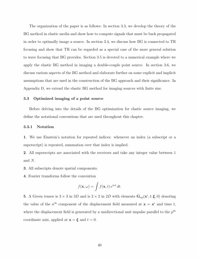
The organization of the paper is as follows: In section 3.3, we develop the theory of the
BG method in elastic media and show how to compute signals that must be back propagated
in order to optimally image a source. In section 3.4, we discuss how BG is connected to TR
focusing and show that TR can be regarded as a special case of the more general solution
to wave focusing that BG provides. Section 3.5 is devoted to a numerical example where we
apply the elastic BG method in imaging a double-couple point source. In section 3.6, we
discuss various aspects of the BG method and elaborate further on some explicit and implicit
assumptions that are used in the construction of the BG approach and their significance. In
Appendix D, we extend the elastic BG method for imaging sources with finite size.
3.3 Optimized imaging of a point source
Before delving into the details of the BG optimization for elastic source imaging, we
define the notational conventions that are used throughout this chapter.
3.3.1 Notation
1. We use Einstein’s notation for repeated indices: whenever an index (a subscript or a
superscript) is repeated, summation over that index is implied.
2. All superscripts are associated with the receivers and take any integer value between 1
and N .
3. All subscripts denote spatial components.
4. Fourier transforms follow the convention
f(x, ω) =
∫f(x, t) eiωt dt.
5. A Green tensor is 3× 3 in 3D and is 2× 2 in 2D with elements Gnp(xi, t; ξ, 0) denoting
the value of the nth component of the displacement field measured at x = xi and time t,
where the displacement field is generated by a unidirectional unit impulse parallel to the pth
coordinate axis, applied at x = ξ and t = 0.
40
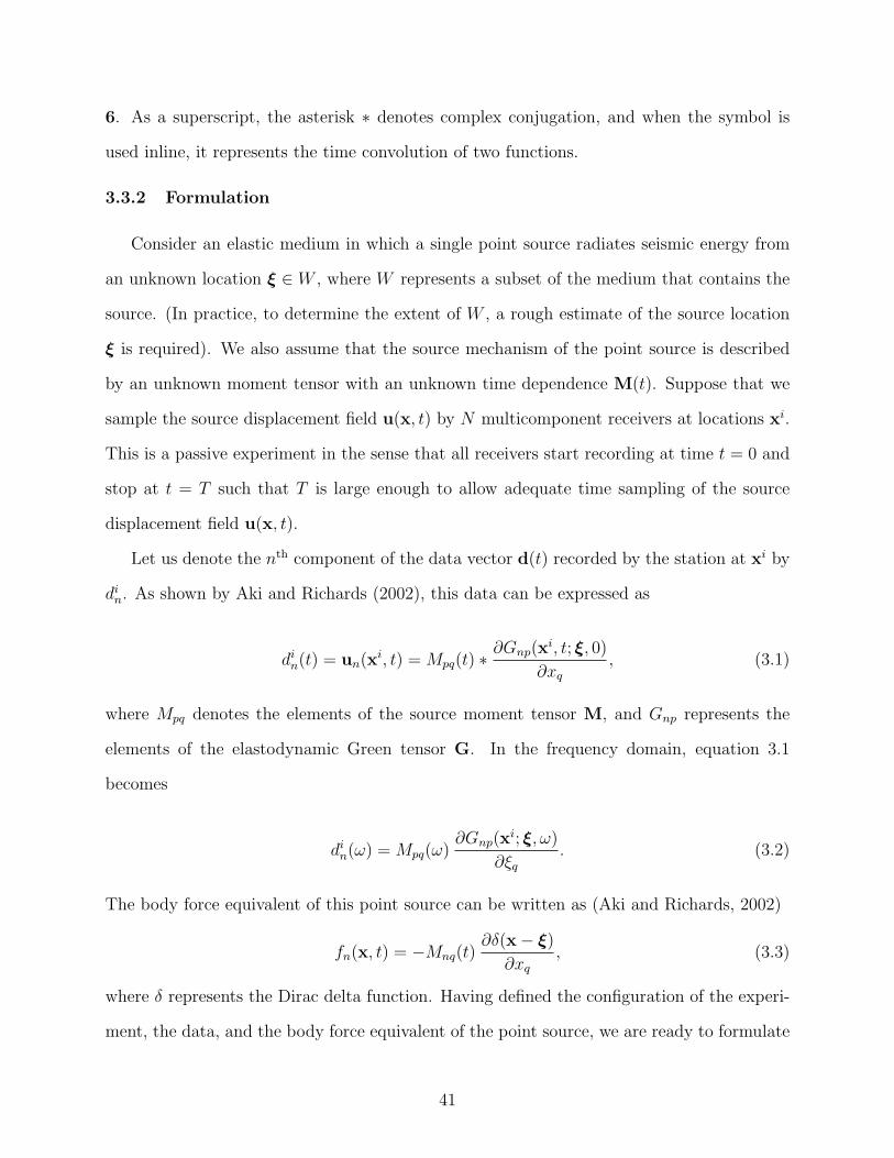
6. As a superscript, the asterisk ∗ denotes complex conjugation, and when the symbol is
used inline, it represents the time convolution of two functions.
3.3.2 Formulation
Consider an elastic medium in which a single point source radiates seismic energy from
an unknown location ξ ∈ W , where W represents a subset of the medium that contains the
source. (In practice, to determine the extent of W , a rough estimate of the source location
ξ is required). We also assume that the source mechanism of the point source is described
by an unknown moment tensor with an unknown time dependence M(t). Suppose that we
sample the source displacement field u(x, t) by N multicomponent receivers at locations xi.
This is a passive experiment in the sense that all receivers start recording at time t = 0 and
stop at t = T such that T is large enough to allow adequate time sampling of the source
displacement field u(x, t).
Let us denote the nth component of the data vector d(t) recorded by the station at xi by
din. As shown by Aki and Richards (2002), this data can be expressed as
din(t) = un(xi, t) = Mpq(t) ∗∂Gnp(x
i, t; ξ, 0)
∂xq, (3.1)
where Mpq denotes the elements of the source moment tensor M, and Gnp represents the
elements of the elastodynamic Green tensor G. In the frequency domain, equation 3.1
becomes
din(ω) = Mpq(ω)∂Gnp(x
i; ξ, ω)
∂ξq. (3.2)
The body force equivalent of this point source can be written as (Aki and Richards, 2002)
fn(x, t) = −Mnq(t)∂δ(x− ξ)
∂xq, (3.3)
where δ represents the Dirac delta function. Having defined the configuration of the experi-
ment, the data, and the body force equivalent of the point source, we are ready to formulate
41
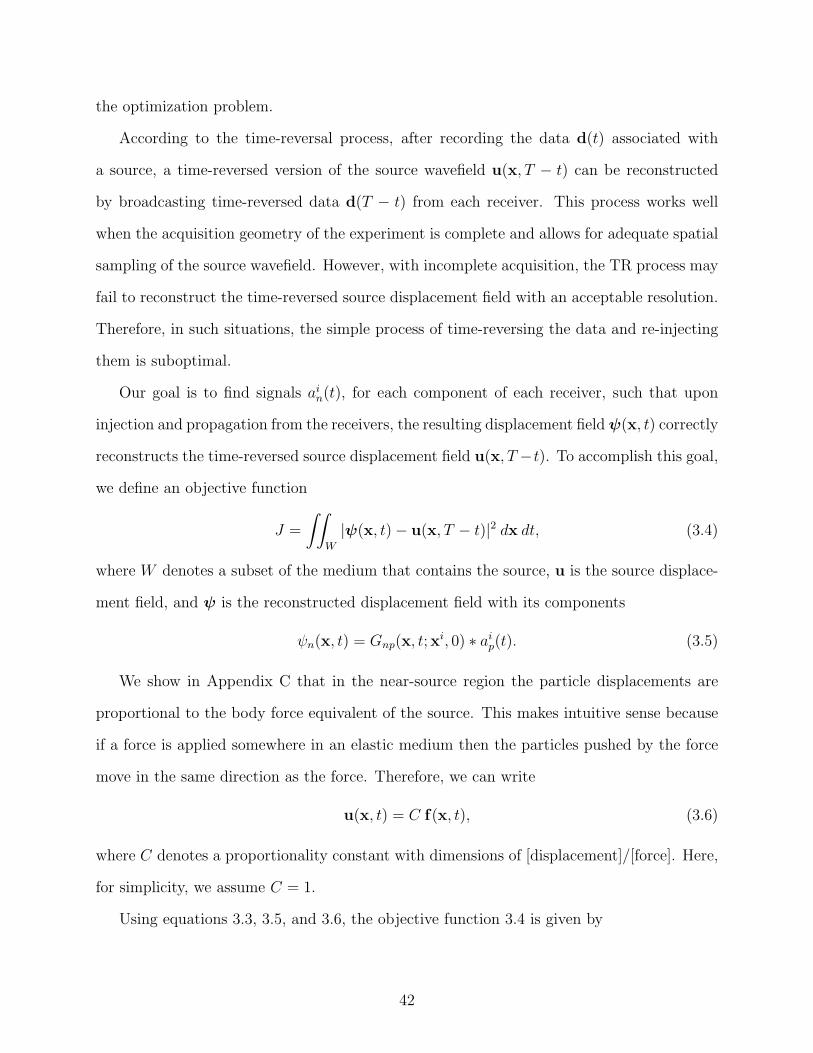
the optimization problem.
According to the time-reversal process, after recording the data d(t) associated with
a source, a time-reversed version of the source wavefield u(x, T − t) can be reconstructed
by broadcasting time-reversed data d(T − t) from each receiver. This process works well
when the acquisition geometry of the experiment is complete and allows for adequate spatial
sampling of the source wavefield. However, with incomplete acquisition, the TR process may
fail to reconstruct the time-reversed source displacement field with an acceptable resolution.
Therefore, in such situations, the simple process of time-reversing the data and re-injecting
them is suboptimal.
Our goal is to find signals ain(t), for each component of each receiver, such that upon
injection and propagation from the receivers, the resulting displacement fieldψ(x, t) correctly
reconstructs the time-reversed source displacement field u(x, T−t). To accomplish this goal,
we define an objective function
J =
∫∫W
|ψ(x, t)− u(x, T − t)|2 dx dt, (3.4)
where W denotes a subset of the medium that contains the source, u is the source displace-
ment field, and ψ is the reconstructed displacement field with its components
ψn(x, t) = Gnp(x, t; xi, 0) ∗ aip(t). (3.5)
We show in Appendix C that in the near-source region the particle displacements are
proportional to the body force equivalent of the source. This makes intuitive sense because
if a force is applied somewhere in an elastic medium then the particles pushed by the force
move in the same direction as the force. Therefore, we can write
u(x, t) = C f(x, t), (3.6)
where C denotes a proportionality constant with dimensions of [displacement]/[force]. Here,
for simplicity, we assume C = 1.
Using equations 3.3, 3.5, and 3.6, the objective function 3.4 is given by
42
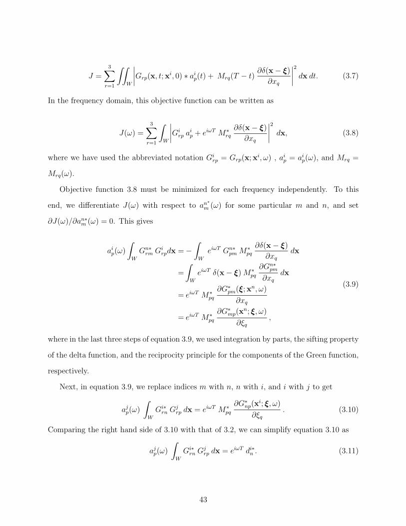
J =3∑r=1
∫∫W
∣∣∣∣Grp(x, t; xi, 0) ∗ aip(t) + Mrq(T − t)
∂δ(x− ξ)
∂xq
∣∣∣∣2 dx dt. (3.7)
In the frequency domain, this objective function can be written as
J(ω) =3∑r=1
∫W
∣∣∣∣Girp a
ip + eiωT M∗
rq
∂δ(x− ξ)
∂xq
∣∣∣∣2 dx, (3.8)
where we have used the abbreviated notation Girp = Grp(x; xi, ω) , aip = aip(ω), and Mrq =
Mrq(ω).
Objective function 3.8 must be minimized for each frequency independently. To this
end, we differentiate J(ω) with respect to an∗m (ω) for some particular m and n, and set
∂J(ω)/∂an∗m (ω) = 0. This gives
aip(ω)
∫W
Gn∗rm G
irpdx =−
∫W
eiωT Gn∗pmM
∗pq
∂δ(x− ξ)
∂xqdx
=
∫W
eiωT δ(x− ξ)M∗pq
∂Gn∗pm
∂xqdx
= eiωT M∗pq
∂G∗pm(ξ; xn, ω)
∂xq
= eiωT M∗pq
∂G∗mp(xn; ξ, ω)
∂ξq,
(3.9)
where in the last three steps of equation 3.9, we used integration by parts, the sifting property
of the delta function, and the reciprocity principle for the components of the Green function,
respectively.
Next, in equation 3.9, we replace indices m with n, n with i, and i with j to get
ajp(ω)
∫W
Gi∗rn G
jrp dx = eiωT M∗
pq
∂G∗np(xi; ξ, ω)
∂ξq. (3.10)
Comparing the right hand side of 3.10 with that of 3.2, we can simplify equation 3.10 as
ajp(ω)
∫W
Gi∗rn G
jrp dx = eiωT di∗n . (3.11)
43

Equation 3.11 represents a linear system of simultaneous equations that can be concisely
expressed as
Γ(ω) a(ω) = eiωT d∗(ω), (3.12)
which must be independently solved for the vector a(ω) for each frequency. More explicitly,
equation 3.12 can be written (in 3D) as
3N×3N Γ11 Γ12 Γ13
Γ21 Γ22 Γ23
Γ31 Γ32 Γ33
︸ ︷︷ ︸
Γ
3N×1 a1
a2
a3
︸ ︷︷ ︸
a
= eiωT
3N×1 d1
d2
d3
∗︸ ︷︷ ︸
d∗
, (3.13)
in which the 3N × 3N matrix Γ consists of nine N ×N submatrices Γkl defined as
Γijkl =
∫W
Gi∗rk G
jrl dx , (3.14)
the 3N × 1 vector a contains three N × 1 subvectors corresponding to the three components
of the optimized signals
ak =
a1ka2k..aNk
, (3.15)
and the 3N × 1 vector d contains three N × 1 subvectors corresponding to the three com-
ponents of the recorded data
dk =
d1kd2k..dNk
. (3.16)
Note that in equation 3.14, a summation is carried out over the index r.
The significance of equation 3.12 is that Γ on the left hand side of equation 3.12 can
be computed (based on equation 3.14) as long as the medium is known and an estimate of
the source location is available. The right hand side of equation 3.12 depends only on the
44
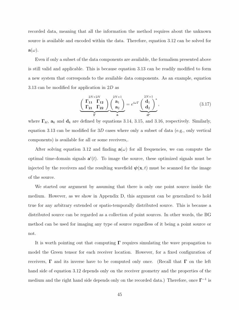
recorded data, meaning that all the information the method requires about the unknown
source is available and encoded within the data. Therefore, equation 3.12 can be solved for
a(ω).
Even if only a subset of the data components are available, the formalism presented above
is still valid and applicable. This is because equation 3.13 can be readily modified to form
a new system that corresponds to the available data components. As an example, equation
3.13 can be modified for application in 2D as
2N×2N(Γ11 Γ12
Γ21 Γ22
)︸ ︷︷ ︸
Γ
2N×1(a1
a2
)︸ ︷︷ ︸
a
= eiωT
2N×1(d1
d2
)∗︸ ︷︷ ︸
d∗
, (3.17)
where Γkl, ak and dk are defined by equations 3.14, 3.15, and 3.16, respectively. Similarly,
equation 3.13 can be modified for 3D cases where only a subset of data (e.g., only vertical
components) is available for all or some receivers,.
After solving equation 3.12 and finding a(ω) for all frequencies, we can compute the
optimal time-domain signals ai(t). To image the source, these optimized signals must be
injected by the receivers and the resulting wavefield ψ(x, t) must be scanned for the image
of the source.
We started our argument by assuming that there is only one point source inside the
medium. However, as we show in Appendix D, this argument can be generalized to hold
true for any arbitrary extended or spatio-temporally distributed source. This is because a
distributed source can be regarded as a collection of point sources. In other words, the BG
method can be used for imaging any type of source regardless of it being a point source or
not.
It is worth pointing out that computing Γ requires simulating the wave propagation to
model the Green tensor for each receiver location. However, for a fixed configuration of
receivers, Γ and its inverse have to be computed only once. (Recall that Γ on the left
hand side of equation 3.12 depends only on the receiver geometry and the properties of the
medium and the right hand side depends only on the recorded data.) Therefore, once Γ−1 is
45

computed and stored, we can reuse it to solve equation 3.12 whenever a new source occurs.
This means that for receivers with a fixed geometry, using BG to image multiple sources can
be computationally very efficient.
3.4 Connection with time reversal
The Backus-Gilbert focusing method, introduced in section 3.3, provides a more general
solution to the wave-focusing problem compared to TR focusing. In fact, there is a close
mathematical relationship between these methods. To be able to see the connection between
BG and TR, we discuss the structure of Γ and examine the significance of its 9 subma-
trices (shown in equation 3.13) to develop a better understanding of their function in the
optimization process.
All elements of Γ hold information about the configuration of the focusing experiment,
i.e., the relative positions of the stations with respect to the inhomogeneities in the propa-
gation medium and the focusing target. The role of the submatrix Γkl can be described as
determining how the signal injected by the kth component of each receiver must be adjusted
with respect to the signals emitted by the lth components of the other receivers in order to
optimally reconstruct the source displacement field. For example, the diagonal submatrix
Γ11 adjusts the signal emitted by the 1st component of each receiver with respect to the 1st
signal injected by other receivers. In contrast, the off-diagonal submatrix Γ32 is responsible
for adjusting the signals emitted by the 3rd component of each receiver with respect to signals
emitted by the 2nd component of the other receivers. A quick inspection of equation 3.14
reveals that Γ is, by definition, a Hermitian matrix; this means that for the submatrices of
Γ, we have Γijkl = Γji
lk
∗. Therefore, whatever function or role we attribute to Γkl, the same
function can be assumed for its conjugate transpose matrix Γlk. With this background about
the anatomy of Γ, we are now ready to study the relationship between BG and TR.
Approximating Γ in equation 3.12 by the identity matrix I gives
a(ω) = eiωTd∗(ω). (3.18)
46
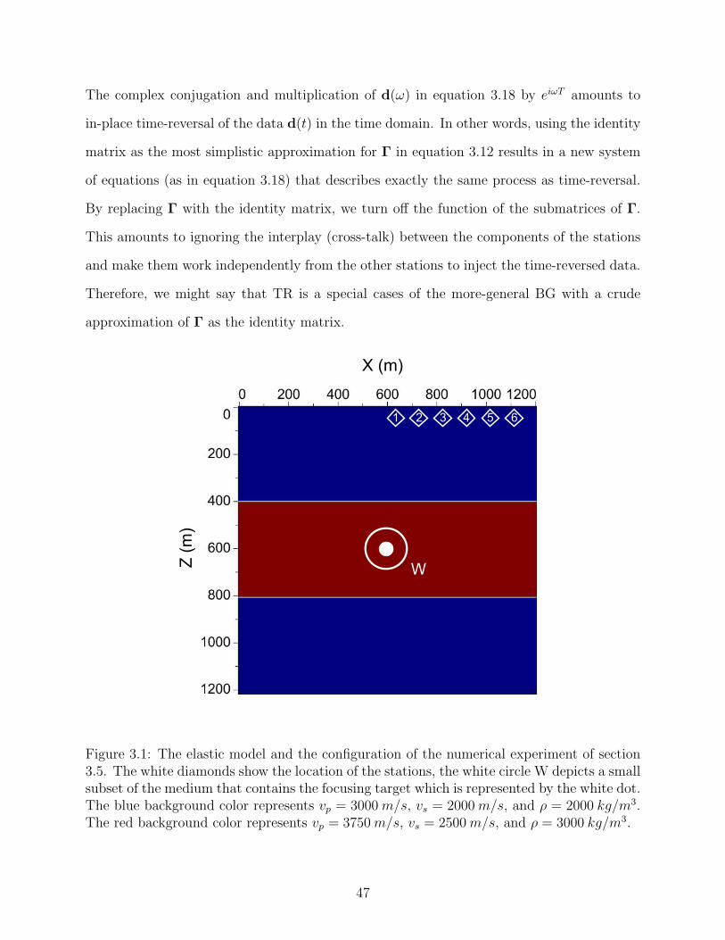
The complex conjugation and multiplication of d(ω) in equation 3.18 by eiωT amounts to
in-place time-reversal of the data d(t) in the time domain. In other words, using the identity
matrix as the most simplistic approximation for Γ in equation 3.12 results in a new system
of equations (as in equation 3.18) that describes exactly the same process as time-reversal.
By replacing Γ with the identity matrix, we turn off the function of the submatrices of Γ.
This amounts to ignoring the interplay (cross-talk) between the components of the stations
and make them work independently from the other stations to inject the time-reversed data.
Therefore, we might say that TR is a special cases of the more-general BG with a crude
approximation of Γ as the identity matrix.
4
5
6
W
X (m)
W
1 2 3 4 5vp = 3000m/s
vs = 2000m/s
vs = 2000m/s
⇢ = 2000 kg/m3
vp = 3000m/s
vs = 2000m/s
⇢ = 2000 kg/m3
Z (m
)
X (m)
W
1 2 3 4 5 6
Figure 3.1: The elastic model and the configuration of the numerical experiment of section3.5. The white diamonds show the location of the stations, the white circle W depicts a smallsubset of the medium that contains the focusing target which is represented by the white dot.The blue background color represents vp = 3000 m/s, vs = 2000 m/s, and ρ = 2000 kg/m3.The red background color represents vp = 3750m/s, vs = 2500m/s, and ρ = 3000 kg/m3.
47

3.5 Numerical experiment
We apply the elastic BG method in a 2D synthetic experiment to image a point source
with a double-couple mechanism and compare the result with the same image produced by
TR. The configuration of the experiment is shown in Figure 3.1. The six diamonds represent
the multicomponent receivers, the white dot depicts the source location, and the white circle
shows the optimization window W , used in the definition of the objective function in equation
3.4. All receivers are at the surface (z = 0m) with the first receiver at x1(x, z) = (630m, 0m)
and the sixth receiver at x6(x, z) = (1110 m, 0 m). Adjacent receivers are 90 m apart. The
earth model used for wave propagation is a heterogeneous elastic 2D model with absorbing
boundaries (Figure 3.1) consisting of three layers. Wave propagation is simulated using an
explicit finite-difference approximation of the 2D elastic isotropic wave equation with an
absorbing boundary condition on a 200 × 201 grid with grid spacings dx = dz = 6 m and
with time step dt = 1ms.
The data vector di(t) is simulated using a horizontal point source of slip with a double-
couple mechanism located at ξ = (600 m, 600 m) within W . The time dependence of the
source is given by a Ricker wavelet with peak frequency of 55Hz and peak time t = 100ms.
We sample the displacement field generated by this source by the six receivers as time signals
din(t), ∀i ∈ {1, 2, ..., 6}, ∀n ∈ {1, 2}, and for 0 < t < T = 0.6s. Here din(t) represents the data
recorded by the nth component of the ith receiver. After simulating the data, for the rest of
the experiment, we pretend that we do not know the exact location and time of the source.
However, we assume that an estimate of the source location is available. This estimate is
needed for defining the integration window W such that it contains the source. Here, W is a
circular area with radius of 90m. The integrand in equation 3.14 is an oscillatory function,
therefore to avoid dominant contribution from the end points, we apply a Gaussian taper to
the edges of integration window W.
To form the matrix Γ, in equation 3.17, we require the Green tensors G(x, t; xi, 0) for
all receivers. We approximate the components of each Green tensor by injecting a band
48
limited spikes with frequencies between 2 Hz and 140 Hz at each receiver location xi and
propagating the wavefield for T = 0.6 s. These wavefields are then Fourier transformed to
the frequency domain and used in equation 3.14 to compute the elements of the 12 × 12
matrix Γ independently for all frequencies within the bandwidth of the experiment.
At this point, we can form the system of equations 3.17 for each frequency independently
and solve the system for ai(ω), the Fourier coefficients of the optimized signals ai(t). These
optimized signals are then broadcast by the receivers to generate the optimal time-reversed
displacement field ψ(x, T−t) that will focus at the correct source location. Note that, in this
2D example, ψ is a vector field with 2 components, a vertical and a horizontal component.
The last step is to scan ψ(x, T − t) to detect and extract the source image which has been
created at location ξ ∈ W and at the correct time associated with the source activation time.
After detecting the source image, the actual source location, time, and the spatio-temporal
characteristics of the source can be inferred from that image.
Possible criteria to detect the source image can include high energy or a particular type
of radiation pattern which is expected for the source. For example, a seismic source with
a double-couple mechanism has a characteristic four-lobe radiation pattern for the P-wave
(radial displacement) component (Aki and Richards, 2002). The P- and S- components of the
displacement field can be readily computed as the curl and divergence of the displacement
field, respectively (Larmat et al., 2009).
Figures 3.2 and 3.3 summarize the results of the numerical experiment described above.
Figure 3.2 consists of two panels. The left panel depicts the vertical component of the
optimal signals in the column labeled BG, and the vertical component of the time-reversed
data in the column labeled TR. Similarly, the right panel depicts the horizontal component
of the optimal signals in the column labeled BG, and the horizontal component of the time-
reversed data in the column labeled TR. The signals in each column (of both panels) have
been normalized by dividing all samples by the maximum absolute value of the amplitude
of all traces in the same column.
49
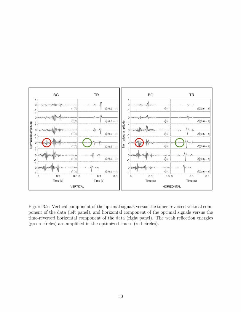
1
-1
0
1
-1
0
1
-1
0
1
-1
0
1
-1
0
1
-1
0
Nor
mal
ized
am
plitu
de
BG TR BG TR
VERTICAL HORIZONTAL
0 0.3Time (s)
0.6 0 0.3Time (s)
0 0.3Time (s)
0 0.3Time (s)
1
-1
0
1
-1
0
1
-1
0
1
-1
0
1
-1
0
1
-1
0
Nor
mal
ized
am
plitu
de
a11(t)
a21(t)
a31(t)
a41(t)
a51(t)
a61(t) a62(t)
a52(t)
a42(t)
a32(t)
a22(t)
a12(t)
0.6 0.6 0.6
d11(0.6� t)
d21(0.6� t)
d31(0.6� t)
d41(0.6� t)
d51(0.6� t)
d61(0.6� t) d62(0.6� t)
d52(0.6� t)
d42(0.6� t)
d32(0.6� t)
d22(0.6� t)
d12(0.6� t)
theta =03 layers
Figure 3.2: Vertical component of the optimal signals versus the timer-reversed vertical com-ponent of the data (left panel), and horizontal component of the optimal signals versus thetime-reversed horizontal component of the data (right panel). The weak reflection energies(green circles) are amplified in the optimized traces (red circles).
50

The optimization process has produced signals that are different from their corresponding
time-reversed data in both amplitude and shape. For example, the small amplitude events in
the time-reversed traces (e.g., the energy encircled in green) correspond to reflected energy
from the discontinuity at z = 800m in Figure 3.1. Note how the same reflected events (i.e.,
the energy encircled in red) are amplified by BG in the optimally computed signals.
Figures 3.3a and 3.3b depict the divergence (radial component or P-wave) and curl (trans-
verse component or S-wave) of the source displacement field enclosed within W at the activa-
tion time of the double-couple point source. We can think of Figure 3.3a as the exact (true)
P-wave image and of Figure 3.3b as the exact (true) S-wave image of the source wavefield.
The radial and transverse component of the optimally reconstructed source displacement
field ψ(x, T − t) at the time of focus are shown in Figures 3.3c and 3.3d, respectively. These
are the P- and S-wave images of the source obtained by taking the divergence and curl,
respectively, of ψ(x, T − t). Finally, the P- and S-wave images of the source produced by TR
are depicted in Figures 3.3e and 3.3f, respectively. The BG images (second row of Figure 3.3)
are superior to the TR images (third row). Note how the four lobes of the P-wave radiation
pattern are resolved by BG in Figure 3.3c, whereas it is impossible to recognize them in
the corresponding TR image in Figure 3.3e. The four-lobe S-wave radiation pattern is not
resolved by either BG or TR. Nevertheless, compared to the TR image (3.3f), the BG image
(3.3d) resembles the exact S-wave image (3.3b) more closely in both size and orientation.
The improvement of the resolution in the BG images, can be attributed to a more bal-
anced illumination of the target. This is made possible by using the amplified reflected events
in the optimized signals shown in Figure 3.2. When the optimized signals are propagated,
a strong coherent burst of energy is create by these amplified events. This coherent energy
travels in advance of the direct arrival energy and part of it, after bouncing off the reflector
at z = 800 m, illuminates the target from underneath. Of course, BG did not create this
energy out of nowhere. The energy is also present in the TR experiment, but it is much
weaker. The observed improvement is mostly the result of detecting this weak energy by
51

BG and properly amplifying it in order to balance the target illumination. Effectively, this
is equivalent of using the reflector at z = 800m as an elastic mirror in order to augment the
illumination angles, which in the case of TR are limited to the small angle subtended by the
first and the last receivers.
Z (m
)
Nor
mal
ized
am
plitu
de
1
0
-1
X (m)
520 600 680
520
600
680
X (m)
520 600 680
Z (m
)
520
600
680
Z (m
)
520
600
680
BG
TR
BG
TR
srcsrc
theta =03 layers
(a) (b)
(c) (d)
(e) (f)
CURLDIVERGENCE
Figure 3.3: Divergence (a) and curl (b) components of the source displacement field enclosedwithin W at the activation time of the source are compared with the P-wave (c) and S-wave(d) images of the source produced by BG, and with the P-wave (e) and S-wave (f) imagesof the source produced by TR.
52
3.6 Discussion
The success of the BG method in producing accurate source images depends on the
validity of the assumptions that were made in formulating the method. The most significant
of these assumptions are knowledge of the elastic medium (e.g., P- and S-wave velocities and
density) and an approximate location of the source. In Chapter 2, we used numerical tests
to study the sensitivity of the acoustic BG method to inaccuracies in the velocity model,
uncertainty in the source location which determines the size of the optimization window
W , and the presence of noise in data. Similar tests for the elastic BG focusing lead to
similar conclusions as were reported in the acoustic case. Here, without going into details,
we summarize the main conclusions of the numerical sensitivity tests for the elastic BG. We
will return to these tests and analyze them more thoroughly in the next chapter.
In any source-imaging method, using an inaccurate model leads to the mislocation of the
source or degradation of the source image. BG focusing is not an exception in this respect.
As shown by the example in section 3.5, BG relies on utilizing the scattered energy in data
in order to compensate for the incomplete acquisition. In this case, to effectively balance
the illumination, BG requires an accurate velocity model that contains the reflectors that
are associated with the reflection energy recorded in the data. Otherwise, if the model is not
sufficiently accurate, BG will not be as effective as it is portrayed by the example in section
3.5 and, depending on the accuracy of the velocity model, the BG image of the source may
be degraded. In our tests, where the velocity models used by BG are moderately perturbed
from the true model (e.g., 10% velocity error or mislocation of the reflecting interfaces), the
obtained BG images are less focused compared to the case were the true velocity is used.
Nevertheless, they are still more focused than the corresponding TR images.
To use the BG method, we also need an estimate of the source location such that we
can be certain that the source is somewhere within a limited area W . In practice, such an
estimate of the source location is usually available. For instance, in earthquake seismology,
the approximate location of the source can be obtained using simple inversion techniques for
53
source location (Stein and Wysession, 2003). Similarly, in hydraulic fracturing monitoring
surveys, geophysicists often have a good estimate of the size of the affected area around the
injection well where microseismic energy is most likely to originate. The size of W is an
important factor in determining the effectiveness of BG as a source-imaging method. With a
limited number of receivers, the smaller W (the smaller the uncertainty in the location of the
source) is, the easier it is to minimize the BG objective function (equation 3.4). However,
there is a lower limit on how small W can be to obtain best focusing results. The optimum
focusing results are achieved when the size for the optimization window W is 2 to 3 times
the dominant wavelength in the data. Using larger windows results in less focused (however
still better than TR) source images. Note that the size of W also depends on the accuracy
of the velocity model. This is because velocity errors could lead to mislocation of the source.
Therefore, the size of W must chosen taking the uncertainties in the velocity model into
account such that W is large enough to contain the mislocated source.
The presence of noise in the recorded data is an important matter that needs to be
carefully addressed. In our numerical example of section 3.5, we did not include noise.
Applying the BG method for source imaging depends on the validity of equation 3.12 which
allows us to solve for optimal signals without explicit knowledge of the source parameters.
However, in a real source-imaging scenario, equation 3.12 does not hold exactly because
recorded data always contain noise. Therefore, equation 3.12 must be replaced by
Γ(ω)a(ω) ≈ eiωT (d∗(ω) + η∗(ω)), (3.19)
where η denotes the noise vector and d the theoretical noise-free data described by equation
3.2.
The stability of the solution a in equation 3.19 depends on the condition number of Γ(ω),
which itself depends on the configuration of the receivers, the properties of the medium,
and the frequency ω for which Γ(ω) is computed. If Γ(ω) is ill-conditioned, then some
regularization technique, e.g., truncated singular value decomposition (TSVD), can be used
54

to find a stable solution to equation 3.19. With a proper amount of regularization, BG can
tolerate noise in data. The stronger the noise level is, the more regularization is required to
obtain stable results. However, too much regularization degrades the source image. Based
on our tests (see Chapter 4), applying BG on noisy data with signal to noise ratio as low as
1 can still yield well focused images, however, stronger noise levels makes the source image
noisy and hard to detect.
3.7 Conclusion
Time-reversal (TR) focusing methods rely on the time-reversal invariance of the wave
operator. When acquisition is incomplete, source-imaging techniques based on time-reversal
focusing are not optimal. In this paper, to overcome the limitations imposed by incomplete
acquisition, we approach source imaging in elastic media as an optimization problem. The
new approach, named Backus-Gilbert focusing (BG), provides a more general solution to
elastic wave focusing than TR does.
To apply BG in source imaging, the medium must be known and also an estimate of
the source position must be available. Apart from these two requirements, no other a priori
information is needed by the method. Of course, since the method is formulated as an
inverse problem that relies on the knowledge of the medium, it is more sensitive than TR
to inaccuracies in the model. We showed with a numerical example simulating an elastic
source-imaging experiment with sparse and limited-aperture receiver geometry, that BG can
produce better resolved images of an unknown source than TR. For source imaging using
receiver stations with a fixed geometry, the application of the method can be computationally
efficient.
One area of geophysics that is a good candidate for application of BG is imaging earth-
quake sources. This is because of three reasons: first, a relatively reliable elastic model of
the earth is available in global seismology which can be used by BG. Second, the advantages
of BG over TR are most pronounced in experiments with incomplete acquisition geometry.
The global network of seismometers does not have a uniform distribution on the Earth and
55

therefore earthquakes that occur in certain poorly-instrumented areas cannot be recorded
properly. Finally, the data quality in terms of signal-to-noise ratio for the strong earthquakes
recorded in global seismology are often very good, thereby minimizing the effects of noisy
data on the BG method discussed above.
3.8 Acknowledgments
This research was supported by the sponsor companies of the Consortium Project on
Seismic Inverse Methods for Complex Structures. We are especially thankful to Dr. Jon
Sheiman for supporting us with invaluable insights. The software used to produce the results
in the paper was written in Java and Jython with the use of libraries in the Mines Java Toolkit
freely available at https://github.com/dhale/jtk.
56

CHAPTER 4
BACKUS-GILBERT SOURCE IMAGING: SENSITIVITY ANALYSES
A paper to be submitted to the Geophysical Journal International
Farhad Bazargani1 and Roel Snieder1
4.1 Abstract
Seismic source imaging can be viewed as an under-determined linear inverse problem with
infinitely many potential solutions. The Backus-Gilbert method is designed to optimize the
resolution of the inverse problem and gives the minimum L2-norm solution. Considering
the Backus-Gilbert method in the framework of inverse theory facilitates analyzing the pos-
sibilities and limitations of the method using the available tools in inverse theory. Using
elastic source-imaging simulations, we analyse the sensitivity of the Backus-Gilbert method
to errors in the earth model and noise in data. We also study how the source image obtained
by the method is affected by the size of the model space which is determined by the size
of the monitored region. Finally, we examine the resolution of the Backus-Gilbert method
using synthetic tests with various source-receiver configurations.
4.2 Source imaging as an inverse problem
In seismic source estimation, we are interested in monitoring a specific area W for seismic
activity in order to characterize the sources originated from that area. The seismic activity
is recorded using a limited number of receivers, N . Receiver locations are given by xi, i =
1, 2, ..., N and each records data passively for T seconds. We usually assume that the elastic
properties of the medium are known so that we can accurately model the wave propagation
inside the medium.
1Center for Wave Phenomena, Colorado School of Mines, Golden, Colorado 80401, USA
57
The source can be located anywhere inside the monitored region with an arbitrary spatio-
temporal character. We can model a source, in the most general sense, as a succession of
point sources that occur at locations ξ, and with moment tensors M(ξ, t) defined for all
ξ ∈ W and t ∈ [0, T ], and write
M(x, t) =
∫W
M(ξ, t) δ(x− ξ) dξ . (4.1)
Equation 4.1 implies that the source is considered to be made of many virtual point sources
at every location inside W . The objective is to characterize the actual seismic source by
determining the behaviour of each of these virtual point sources.
The nth component of the data vector d(t) associated with the seismic source and recorded
by the station at xi can be expressed as
din(t) =
∫Mpq(ξ, t) ∗
∂Gnp(xi, t; ξ, 0)
∂ξqdξ, (4.2)
where summation over repeated indices is implied, Mpq(ξ, t) denotes the elements of the
moment tensor M of the virtual point source at ξ, and Gnp(xi, t; ξ, 0) represents the elements
of the elastodynamic Green tensor associated with an impulsive source at ξ and recorded by
the receiver at xi. We are temporarily ignoring the presence of noise in data but will return
to it later in section 4.3.3. Equation 4.2 defines a linear process that can be discretized and
expressed in the frequency domain using the vector matrix notation
d = G m, (4.3)
where dn×1 is the data vector, Gn×m is the data kernel, and mm×1 in the unknown model
vector. Here, n is the dimension of the data space which isN times the number of components
in each receiver. m represents the dimension of model space which is equal to the number
of virtual sources that we imagine at each grid point within the monitoring area times the
number of unknown parameters for each virtual source.
58
Our goal is to invert equation 4.3 to find an estimate m of the true model m. In a typical
source-imaging problem the number of receivers is limited. This means n < m and therefore
Gn×m is a non-square matrix and formally not-invertible. Nonetheless, it is possible to find
an inverse mapping from the data to the estimated model. The most general linear mapping
from the data to the estimated model can be expressed as
m = G−g d, (4.4)
where the generic m×n matrix G−g denotes the generalized inverse of G. There are several
ways for designing the inverse operator G−g for the under-determined system of equation
4.3 (Snieder and Trampert, 1999). One way is through the approach introduced by Backus
and Gilbert in 1960s (Backus and Gilbert, 1968; Aki and Richards, 1980). Here, we briefly
review this method.
4.2.1 The method of Backus and Gilbert
Let us start by inserting d from equation 4.3 into 4.4 to obtain
m = G−gGm = R m, (4.5)
where the m×m matrix R = G−gG is the averaging kernel or the model resolution matrix.
Note that, in equation 4.5, R = I would imply perfect resolution, i.e., m = m which amounts
to no averaging and a one-to-one correspondence between the elements of vectors m and m.
However, with incomplete acquisition, perfect resolution is not possible and R 6= I. The
structure of R and how closely it resembles the identity matrix ultimately depends on the
configuration of the experiment which is captured by the data kernel G. The closer R
resembles I, the better is the resolution of the estimated solution m. This can be used as a
criterion to specify the generalized inverse G−g. In other words, we can determine G−g by
requiring that R should resemble the identity matrix Im×m as closely as possible. This is
achieved by defining and minimizing an objective function
J = ‖R− I‖2, (4.6)
59

where ‖.‖2 denotes the matrix (Frobenius) norm here. Minimizing J with respect to the
components of G−g gives (Tarantola, 2005)
G−gBG = G†(GG†)−1, (4.7)
where G−gBG denotes the particular generalized inverse obtained through the Backus-Gilbert
approach. Then for the model resolution matrix we have
RBG = G−gBGG = G†(GG†)−1G. (4.8)
Combining 4.5 and 4.8, gives
mBG = RBG m = G†(GG†)−1Gm, (4.9)
which can be simplified using 4.3 as
mBG = G†(GG†)−1d, (4.10)
where mBG denotes the estimated model that is obtained using the Backus-Gilbert method.
Before we interpret the significance of this model estimate, we must explain that the way
we derive and implement the Backus-Gilbert method in chapters 2 and 3 for source imaging
is slightly different from the usual approach explained above. That is, instead of designing
the generalized inverse operator through minimizing objective function 4.6, we solve for the
optimized signals a that must be injected by each receiver for best focusing result. This is
done through minimizing a different objective function defined as
J′ = ‖GTa− eiωTm∗‖2. (4.11)
Minimizing 4.11 with respect to a gives
a = eiωT (G∗GT )−1d∗, (4.12)
60

The model estimate (source image) is then obtained by back propagating a given by equation
4.12, i.e.,
m′BG = GTa = eiωTGT (G∗GT )−1d∗. (4.13)
Note that the model estimate m′BG in 4.13 is the complex conjugate of mBG in equation 4.10
with a phase shift. This complex conjugation in the frequency domain is equivalent of time-
reversal in the time domain. In other words, the model estimate in 4.13 is the time-reversed
version of 4.10, otherwise they are identical. Finally, note that approximating G∗GT by the
identity matrix in equation 4.13 gives the time-reversal (TR) solution, i.e.,
mTR = eiωTd∗. (4.14)
4.2.2 The minimum norm solution
As mentioned before, equation 4.3 with m < n describes an under-determined system
of equations with non-unique solutions. To resolve this non-uniqueness, we must add to
the problem some a-priori information or assumption about the solution. For example, one
possible a-priori assumption could be based on the simplicity of the solution (Menke, 2012).
Put another way, simplicity of the solution can be used as a criterion to single out one
solution as the best among the infinitely many possible solutions to the under-determined
inverse problem.
The notion of simplicity can be quantified by some measure of length (say L2-norm) of
the solution. For example, the minimum norm solution to equation 4.3 is a model estimate
mMN that minimizes ‖m‖2 subject to ‖d−Gm‖2 = 0. This minimization problem can be
solved using the method of Lagrange multipliers (Menke, 2012). The solution is
mMN = G† (GG†)−1 d. (4.15)
61
Comparing the right hand side in equation 4.10 with that in 4.15, we find that mBG = mMN ;
that is the Backus-Gilbert solution is indeed the same as the minimum L2-norm solution.
Note that if GG† in equations 4.10 and 4.15 is singular (non invertible) then it must be
regularized to remove the singularity. In that case, the regularized solution will not be
exactly the minimum norm solution and the resolution degrades. We further discuss this
issue in section 4.3.3.
The fact that mBG = mMN implies that if the true model is more complicated than the
minimum norm solution, then the BG method will not be able to recover it exactly. For
example, consider the case where the true model contains some components m0 in the null
space of G, i.e., m = mMN + m0. Then one can see from equation 4.9 that m0 would be
annihilated by G and cannot affect the estimated model (in fact, it would not be sensed by
the receivers and affect the data in the first place). What is recoverable by the BG method
is then the minimum length part mMN of the true model.
Some important questions may arise regarding the justification of the minimum norm
criterion. For example, one might ask whether simplicity is a justifiable criterion for resolving
non-uniqueness in the source estimation problem, or whether the L2-norm of the model is
a proper measure to quantify the notion of simplicity of the model. Using simplicity as
a-priori information in an inverse problem is based on the philosophical argument (Occam’s
razor) that the simpler explanation should be preferred to more complicated explanations
(Aster et al., 2013). Although, the reality might prove to be not so simple, in the absence
of certainty, explaining a phenomenon with the fewest assumptions is both reasonable and
aesthetically appealing. Using the L2-norm of the model as a measure for assessing simplicity
is not necessarily realistic either. The sparsity-promoting L1-norm, for example, could be
another viable candidate for measuring model simplicity. However, compared to L2-norms,
solving an optimization problem involving L1-norms is generally more challenging.
If more accurate a-priori information about the model is available, more complicated
measures of simplicity can be used to resolve the non-uniqueness or inconsistency in the
62
inverse problem. For instance, a-priori information such as data and model covariances, if
available, may be incorporated in the problem by defining a more appropriate metric for the
L2-norm in a weighted least squares scheme (Jackson, 1979; Snieder and Trampert, 1999).
4.3 Sensitivity tests and analyses
In the previous section, we re-examined the Backus-Gilbert source-imaging method in an
abstract sense to put it in the context of inverse theory. Doing so allows us to develop a deeper
understanding of the BG method and its limitations and possibilities. It also facilitates
analysing the sensitivity of the method to parameters such as the physical properties of the
propagating medium, size of the monitoring area (optimization window), and noise. Here,
we test the behaviour of the BG method in several numerical simulations and interpret the
outcome of the tests in the light of the theoretical insight gained in section 4.2.
For the first series of tests, we use the source-receiver configuration and the three-layer
elastic earth model shown in Figure 4.1. The diamonds represent the receivers, the white dot
denotes the location of the source, and the white circle depicts the extent of the optimization
window (monitoring area) W . All receivers are at the surface (z = 0m) with the first receiver
at x1(x, z) = (630 m, 0 m) and the sixth receiver at x6(x, z) = (1110 m, 0 m). Adjacent
receivers are 90m apart. All boundaries of the earth model are assumed to be non-reflective
(absorbing). Wave propagation is simulated using an explicit finite-difference approximation
of the 2D elastic isotropic wave equation with an absorbing boundary condition on a 200×201
grid with grid spacings dx = dz = 6m and with time step dt = 1ms.
We simulate the data using an isotropic point source located at the white dot in Figure
4.1. The time dependence of the source is given by a Ricker wavelet with peak frequency of
55 Hz and peak time at t = 100 ms. The true P-wave image of this isotropic point source
is shown in Figure 4.2a. Here, by true P-wave image, we mean the image that one would
obtain in a full-aperture TR experiment by computing the divergence of the back propagated
displacement field at the time of focus. The true image therefore represents the TR image
of the point source for a perfect aperture (receivers placed equidistantly at a spacing of
63
60 m along the boundary of the computational domain in Figure 4.1). The reason for not
showing the S-wave image of the source in Figure 4.2 is that the isotropic point source in
this experiment does not generate S-waves at its activation time.
Before carrying out the sensitivity tests, we use the simulated data (with no added noise)
to image the source using the TR method with the source-receiver configuration and the
earth model of Figure 4.1 (henceforth the true earth model). The resulting TR image of the
source is shown in Figure 4.2b. The quantity Q shown in this figure is the measure introduced
in Chapter 2 to quantify the spread of energy in the image of a point source. The smaller Q
is, the more focused and localized is the image. Figure 4.2c shows the image of the source
obtained using the BG method with the true velocity model and with W of radius 90m. We
then repeat this source-imaging test using the BG method applied partially by zeroing out
the off-diagonal elements in each submatrix of Γ in equation 3.17. This amounts to forcing
BG to optimize the injected signals using the components within each receiver independently
of the other receivers and hence, ignoring the interplay of the receiver components among
different stations. The source image obtained by this experiment is shown in Figure 4.2d.
A comparison of the images shown in Figures 4.2b-d demonstrates that the BG method,
compared to TR, produces more focused images. It also indicates that to be most effective,
the BG optimization process must take the interplay among the components of different
receivers into account. We next analyze the sensitivity of the BG method to inaccuracies in
the earth model.
4.3.1 Earth model and the data kernel
The solution of the BG method, as shown by equation 4.10, is expressible in term of
the data kernel G and the data d. Therefore, the accuracy of our knowledge of G closely
affects the quality of the solution obtained by BG. Note that G is the forward modeling
operator that captures the physics of the forward experiment which, in this case, consists of
generation, propagation, and recording of the elastic waves. The accuracy of G depends on
two major factors. The first contributing factor is the physics that is used to model the ex-
64

4
5
6
W
X (m)
W
1 2 3 4 5vp = 3000m/s
vs = 2000m/s
vs = 2000m/s
⇢ = 2000 kg/m3
vp = 3000m/s
vs = 2000m/s
⇢ = 2000 kg/m3
Z (m
)
X (m)
W
1 2 3 4 5 6
Figure 4.1: The elastic earth model and the source-receiver configuration for the numericalsensitivity tests discussed in the text. The white diamonds show the location of the receivers,the white circle W depicts a small subset of the medium (monitoring area) that containsthe point source represented by the white dot. The blue background color represents vp =3000 m/s, vs = 2000 m/s, and ρ = 2000 kg/m3. The red background color representsvp = 3750m/s, vs = 2500m/s, and ρ = 3000 kg/m3.
65

Nor
mal
ized
am
plitu
de
Z(m
)
X(m)
600 660
540
600
660
-1
1
0.5
0
-0.5
a) b) d)c)
i) j) k) l)
h)e)
m) n) o) p)
a: true velb: true smooth velc: vl=1700d: vl = 1600e: ll = z(ll) -15f: ll = z(ll) +15g: ul = z(ul)-15h: ul = z(ul)+15i: w=30j: w=45k: s/n = 1l: s/n = 2 m: tbg ite=2n: tbg ite= 10o: tbg ite = 15p: tbg ite = 20
f) g)
Q=24.9 m Q=28.1 m Q=28.5 m Q=30.8 m
Q=36.9 m Q=26.5 m
Q=30.9 m Q=30.6 m Q=28.0 m Q=27.9 m
Q=27.3 mQ=31.0 m Q=29.8 m Q=27.8 m
Q=31.5 m
smooth velocitylayer v = -10%
base reflector -60 m base reflector +60 m top reflector -60 m
radius of W = 120 m radius of W = 180 m S/N = 2 S/N = 1
top reflector +60 m
540
layer v = -5% layer v = +5%
Z(m
)
540
600
660
Z(m
)
540
600
660
Z(m
)
540
600
660
X(m)
600 660540
X(m)
600 660540
X(m)
600 660540
TR BG diagonalBG
Figure 4.2: P-wave images of the point source associated with the source-receiver configura-tion depicted in Figure 4.1 showing (a) the true P-wave image of the isotropic point source,(b) TR image using true velocity, (c) BG image using true velocity and optimization win-dow with radius 90 m, (d) BG image where BG is applied partially such that the interplaybetween receiver components among different stations is ignored, (e) BG image using a per-turbed model where the density and velocities of the middle layer are decreased by 10%, (f)BG image using a perturbed model where the density and velocities of the middle layer aredecreased by 5%, (g) BG image using a perturbed model where the density and velocities ofthe middle layer are increased by 5%, (h) BG image using a perturbed model by smoothingthe true velocity with a Gaussian filter, (i) BG image using a perturbed model where thewidth of the middle layer is altered by lowering its base interface by 60m, and (j) by raisingits base interface by 60 m, and (k) by lowering its top interface by 60 m, and (l) by raisingits top interface by 60m, (m) BG image using the true velocity and optimization window Wwith radius 120 m, (n) BG image using the true velocity and optimization window W withradius 180 m, (o) BG image using the true velocity and data contaminated by noise withS/N = 2, and (o) BG image using the true velocity and data contaminated by noise withS/N = 1. All images are obtained by computing the divergence of the injected wavefield atthe time of focus.
66

periment, e.g., the wave equation used to describe wave propagation in the medium. Ideally,
this modeling must be sophisticated enough to describe the actual physical process with suf-
ficient accuracy. The second factor in determining the accuracy of the G is the accuracy of
the information about the elastic properties of the propagating medium. These two factors
can be related in the sense that the level of sophistication in wave propagation modeling
must be commensurate with the level and accuracy of our knowledge of the properties of the
medium. For example, when the medium is anisotropic, one must ideally use an anisotropic
wave equation to accurately model the wave propagation in the medium. However, if infor-
mation about the anisotropic parameters of the medium are poor or absent, then it might
be beneficial to use the simpler but more robust isotropic elastic wave equation.
Assuming that proper physics is chosen for modeling the forward problem, then the
accuracy of the wave propagation parameters of the medium, e.g., velocity and density, is
the dominant factor in determining the success of the BG method. In any source-imaging
method, errors in the velocity model can cause the source image to be created at a wrong
location or time. The BG method is not an exception in this regard. Here we test the effect
of using an erroneous earth model in the BG method. By erroneous, we mean an earth model
that is perturbed and somehow different compared to the true earth model (the model that
was used to simulate data).
We first perturb the earth model by changing the density, and the P- and S-wave veloc-
ities of the middle layer in Figure 4.1 by a fixed amount. Figures 4.2e-g show the P-wave
images of the source as obtained in such tests where the perturbed earth model is constructed
by changing the density and velocities of the middle layer by −10%, −5%, and +5%, respec-
tively. The time and location of the source in these tests are detected automatically using
the maximum energy criterion introduced in Section 2.6.
The elastic BG method utilizes the reflected waves in the data to augment the incom-
plete acquisition (see Chapter 3). Therefore, it is important that the earth model used to
compute the forward operator G in BG contains the major reflectors in the medium with
67

correct reflective strength in their correct position. To test the sensitivity of the method
to inaccuracies in the reflection coefficient of the reflectors, we perturb the earth model by
smoothing it with a Gaussian smoothing filter with standard width of 12 meters. Smoothing
the earth model decreases the impedance contrast across the reflecting interfaces and leads
to weaker reflected energy from the interfaces in the model. For example, after smoothing,
the PP reflected amplitude recorded by the vertical component of receiver 1 in Figure 4.1
decreases about 80%. The P-wave source image obtained by BG using this smoothed veloc-
ity model is shown in Figure 4.2h. More severe smoothing of the earth model leads to more
degradation of the focus quality. Next, we perturb the earth model by changing the depth of
the interfaces in the true model. Figures 4.2i and j are source images obtained by BG using
models that are perturbed by lowering and raising the base reflector of the middle layer in
Figure 4.1 by −60m and +60m, respectively. Figures 4.2k and l show the result of similar
tests for perturbations in the depth of the top interface of the middle layer by −60 m and
+60m, respectively.
As implied by the Q measure associated with source images in Figures 4.2e-l, the quality
of the focus deteriorates as a result of error in the earth model, however, the BG images
obtained with the perturbed earth models in these examples are still more focused than the
TR image (Figure 4.2b). Note that error in the earth model causes the image to focus at
a wrong location, (e.g., see Figure 4.2i). It is important that this error in the location of
the source is not larger than the extent of the optimization window W . In other words, the
maximum tolerable error in the earth model is related to the size of W and can be limited
by it.
4.3.2 The optimization window
The optimization area W in BG source imaging is defined as the area that is known to
contain the source. The position of W can be chosen based on some a-priori information or
estimate about the source location. The size of W must be determined based on the amount
of certainty in the a-priori estimate of source location.
68

To test how the BG source image is affected by the size of W , we repeat the BG imaging
of the point source that was shown in Figure 4.2c but with larger sizes of W . Figures 4.2m
and n show the BG images obtained by these experiments wherein the radius of W is chosen
to be 120m and 180m, respectively. It is evident by these tests that source image obtained
by BG depends on the size of W . More tests like the ones shown above indicate that the best
focusing results are obtained when the radius of the circular window defining W is about
two to three times the dominant wavelength in the experiment.
To see the reason for the dependence of the BG source image on the size of W , recall from
section 4.2 that the size of the optimization area defines the dimension of the model space.
Also recall that the solution provided by the BG method is the simplest model that could
explain the data, which is one solution within W with minimum L2-norm among infinitely
many possible solutions in the model space. This means that the definition of the minimum
norm solution changes with the change in the size of W . Apart from this, since the resolution
matrix R is defined over W , the requirement to optimize the resolution matrix in BG (see
equation 4.6) alters with the change in the size of W . It is therefore not surprising that
changing the size of W should alter the solution obtained by the BG method.
4.3.3 Noise
In deriving the solution of the BG method in section 4.2, we assumed the data to be noise
free. Real data, however, is always contaminated with noise. Therefore, we must account for
noise and study the effect of noise on the source-imaging process. In the presence of noise,
equation 4.3 must be modified as
d = G m + η, (4.16)
where η denotes the noise vector. Similarly equation 4.5 changes to
m = G−gG m + G−g η, (4.17)
which can be written using the expression for G−g given by equation 4.7 as
69
m = G†(GG†)−1G m + G†(GG†)−1 η. (4.18)
Equation 4.18 has two terms. The first term describes the filtering of the true model m with
the resolution kernel (blurring) and the second term describes the mapping of noise from data
to the estimated model (error propagation). Note that inverse of the matrix GG† is present in
both blurring and error propagation terms. We have so far implicitly assumed that the source
estimation problem is purely under-determined, implying that GG† is invertible. However, it
is possible that the problem is mixed-determined meaning that GG† is not invertible and the
problem is ill-posed. Even if (GG†)−1 exists, it could be nearly singular so that the problem
is ill-conditioned. The second term in Equation 4.18 clearly shows that the poor condition
of GG† causes magnification of error in the estimated model. To avoid error magnification,
the ill-conditioned problem can be regularized using common techniques such as truncated
singular value decomposition (TSVD), damped SVD, or weighted least squares. In general,
more aggressive regularization leads to more effective noise suppression. However, one must
remember that there is a trade-off between resolution and noise suppression (Aster et al.,
2013). Regardless of the method chosen for regularization, the covariance of the estimated
model is related to the data covariance matrix as
Cov(m) = G−g Cov(d) G−gT , (4.19)
where G−g denotes the regularized version of G−g.
To see how the presence of noise in data can affect the BG method, we contaminated
the simulated data with uncorrelated band-limited Gaussian random noise with the same
bandwidth as data and with signal to noise ratio of 2. We then used the BG method (with
true velocity) to image the source using this noisy data. The P-wave source image obtained
by this experiment is shown in Figure 4.2o. Finally, we repeat this experiment with stronger
noise with signal-to-noise ratio of 1. The P-wave source image obtained by this experiment is
shown in Figure 4.2p. These experiments show that the BG method, if properly regularized,
70

can tolerate the presence of noise in data. To obtain the images in Figures 4.2o and p, we
regularized the BG inverse problem using TSVD. Other regularization techniques such as
damped singular value decomposition yield similar results.
4.3.4 Resolution
The model resolution matrix RBG in equation 4.9 can be regarded as an averaging kernel
that relates the true model m to the estimated model mBG . Note that the resolution matrix
RBG, given by equation 4.8, does not depend on the data and is completely determined
by G which in turn depends on the earth model and the source-receiver configuration of
the experiment. In fact, the structure of RBG and how closely it resembles the identity
matrix contains all the information needed to study the resolution in a given experiment.
Therefore, it can be studied before actually performing the experiment and used as a tool in
the designing phase of a source-imaging experiment. In practice, where the size of the model
space m is large, computing all m×m elements of the model resolution matrix RBG could
become intractable. To find a practical solution to this problem, we note that each row of
RBG corresponds to one model parameter. It is usually sufficient to compute a few rows
of the model resolution matrix corresponding to model parameters at strategically chosen
locations within the model volume (Menke, 2012). Now the question is how can a specific
row of RBG be computed.
It can be shown that the kth row of the model resolution matrix solves the inverse problem
for synthetic data d(k) corresponding to a specific model parameter vector m(k), one that is
zero except for its kth element, which is unity (that is, a unit spike at row k). This suggests
that the kth row of RBG can be interpreted and computed as the impulse response of the BG
method due to an impulsive source located at the corresponding kth element of the model
(Menke, 2012). This is exactly what we have done so far in our numerical tests. For example,
Figure 4.2c is the image of a spatially impulsive point source. It therefore, can be regarded
as the spatial impulse response of the BG method and interpreted as one row of the model
resolution matrix that corresponds to the model parameters associated with the position of
71

X (m) X (m)
BG TR
1 2 3
4 5 6
7 8 9
Z (m
)Z
(m)
X (m)
a)
b) c)
1 2 3
4 5 6
7 8 9
1 2 3
4 5 6
7 8 9
Figure 4.3: Resolution test for the linear receiver geometry. Panel (a) shows the configurationof the receivers (the diamonds) and the trial source locations (9 white dots). Panel (b)contains 9 images which are impulse responses for 9 BG source-imaging experiments, imagingpoint sources at the white dots shown in panel (a). Panel (c) contains 9 images which areimpulse responses for 9 TR source-imaging experiments, imaging point sources at the whitedots shown in panel (a).
72

Z (m
)
X (m) X (m)
BG TR
1 2 3
4 5 6
7 8 9
Z (m
)
X (m)
a)
b) c)
1 2 3
4 5 6
7 8 9
1 2 3
4 5 6
7 8 9
Figure 4.4: Resolution test for the scattered receiver geometry. Panel (a) shows the config-uration of the receivers (the diamonds) and the trial source locations (9 white dots). Panel(b) contains 9 images which are impulse responses for 9 BG source-imaging experiments,imaging point sources at the white dots shown in panel (a). Panel (c) contains 9 imageswhich are impulse responses for 9 TR source-imaging experiments, imaging point sources atthe white dots shown in panel (a).
73

the white dot in Figure 4.1.
To demonstrate the advantages of studying the resolution of a source-imaging experi-
ment with a given earth model and source-receiver configuration, we compute the BG and
TR images associated with point sources at the 9 locations depicted by the white dots in
Figure 4.3a. The BG impulse responses and the corresponding TR impulse responses are
shown in Figures 4.3b and c, respectively. Each of the 9 images shown in Figure 4.3b or c
could be construed as one row of the resolution matrix associated with the corresponding
source location in the model. As illustrated by these images, the resolution in both BG and
TR source-imaging experiments varies with location of the source and the way it is situated
relative to the receivers and the reflecting interfaces in the earth model. Comparing Figures
4.3b and c shows that the resolution achievable by the BG method is generally higher than
that for TR. The noticeable improvement of the BG resolution compared to the TR resolu-
tion, e.g. in locations 1, 2, 4, and 5, is the result of augmentation of the illumination angles
by the reflectors in the velocity model, but even below the lowest reflector the BG images
are more localized that the TR images.
We next repeat the above resolution test for the receiver geometry shown in Figure 4.4a.
The BG impulse responses and the corresponding TR impulse responses obtained in this
experiment are shown in Figures 4.4b and c, respectively. Both BG and TR methods yield
better resolved images in this experiment compared to the images in Figure 4.3. However,
the improvement of resolution in the BG images over TR images in Figure 4.4 is not as
obvious as in Figure 4.3. This is because larger aperture of the receiver array in Figure 4.4a
leads to a more adequate sampling of the wavefield and a better illumination for all 9 source
locations. Because of this better illumination, TR can be more effective with the scattered
receiver geometry in Figure 4.4a compared to the linear receiver geometry in Figure 4.3a.
Apart from the geometry and configuration of the experiment, the ability to properly
image a source could also depend on the source itself and the way it radiates energy. To
illustrate this point, let us go back to the configuration shown in Figure 4.3a and repeat the
74

DIV
ER
GE
NC
EC
UR
L
✓ = 15�✓ = 0� ✓ = 30� ✓ = 45� ✓ = 60� ✓ = 75� ✓ = 90�
✓ = 15�✓ = 0� ✓ = 30� ✓ = 45� ✓ = 60� ✓ = 75� ✓ = 90�
BG
TRU
EB
GTR
UE
TR true
Figure 4.5: Imaging of a double-couple source with different orientations. The orientation ofthe source is specified by the angle θ measured relative to horizontal. The receiver geometryis the same as that shown in Figure 4.3a and the source is at location 4. Top panel: Thefirst row in the top panel shows the divergence of the BG-optimized wavefield at the time offocus (the P-wave image) for different orientations of the double-couple source. The secondrow in the top panel depicts the true P-wave image of the double-couple source with differentorientations of the source. Bottom panel: The first row in the bottom panel shows the curl ofthe BG-optimized wavefield at the time of focus (the S-wave image) for different orientationsof the double-couple source. The second row in the bottom panel depicts the true S-waveimage of the double-couple source with different orientations of the source.
75

source-imaging experiment for a double-couple point source at source position 4. We start
by a horizontal double-couple source with θ = 0, where θ defines the orientation angle of
the source slip measured with respect to horizontal. After imaging the double-couple source,
we rotate its orientation by 15 degrees clockwise and image it again. We repeat this for
θ = 0◦, 15◦, 30◦, 45◦, 60◦, 75◦, and 90◦. The BG images obtained by this process are shown in
Figure 4.5. The top panel in Figure 4.5 shows the divergence (P-wave) and the bottom panel
shows the curl (S-wave) of the back propagated displacement wavefield at the time of focus.
The first row in each panel shows the images produced by the BG method. The second row
depicts the true images of the source and are included as reference. By true image, we mean
the ideal P- or S-wave image of the source obtained by a complete aperture TR experiment.
Consider the BG images in the divergence panel (top panel). At θ = 0◦ the four-lobe
P-wave radiation pattern of the source is clearly resolved. The quality of the P-wave image,
however, degrades as θ increases to 45◦ and then it improves again from θ = 45◦ to θ = 90◦.
Now, consider the BG images in the curl panel (bottom panel). The quality of the S-wave
image is poor initially at θ = 0◦. It then improves as theta increases to 45◦, and degrades
again from θ = 45◦ to θ = 90◦. This behaviour is easy to explain. The BG method can
produced a well resolved P- or S-wave image of the source only if the receivers record the
corresponding energy radiated by the source. For example, at θ = 0◦, the source strongly
radiates P-waves towards the receivers (see the geometry of receivers relative to source point
4 in the configuration of the experiment shown in Figure 4.3a). The opposite of this situation
is true for the S-wave as the source radiates almost no S-wave towards the receivers at θ = 0◦.
As a result, the P-wave image of the source is well resolved at θ = 0◦ while the quality of
the S-wave image is poor. Note that in this 2D example, regardless of the orientation of
the source, the receivers record enough body-wave energy (P- or S- type) so the source
mechanism and its orientations can be inferred from either P- or S-wave image or both.
In a 3D experiment, however, a double-couple source could be oriented in such a way that
it radiates no body waves towards the receivers. (For instance, consider a case where the
76

receivers are situated along the null axis of the body wave radiation pattern of a double-
couple source.) More precisely, if the true source m in equation 4.3 has components in the
null space of the data kernel G, such null space components will not be sensed in the data
and therefore it can not be recovered by the inversion process.
The tests shown in this section are all 2D examples. Seismic source imaging in 3D is more
challenging because adequate sampling of the source wavefield is much harder in 3D than it
is in 2D. In addition, compared to 2D, numerical modeling of 3D wave propagation requires
more computing resources. One way to deal with these problems is to image the seismic
source using only the surface waves. As opposed to body waves, surface waves essentially
propagate in 2D. Therefore, a 3D source-imaging experiment that just uses surface waves
can be treated as a 2D problem (e.g., Larmat et al., 2006). For proper imaging of deep
earthquakes, however, it might be necessary to use body waves.
4.4 Conclusion
Seismic source imaging is a linear inverse problem and, therefore, it can be studied and
analyzed using the tools of the linear inverse theory. We formulated source imaging as
an under-determined inverse problem. One way to find a unique solution for this under-
determine problem is through the method of Backus and Gilbert which works based on the
optimization of the model resolution kernel for a given problem. We showed that the solution
provided by the BG method is indeed the minimum L2-norm solution to the inverse problem
which is the smallest (in the L2-norm sense) among all possible solutions that can explain
the data.
In the second part of the paper, we analyzed the sensitivity of the BG method to errors
in parameters such as the earth model used by the method for modeling wave propagation
and the size of the optimization area. We also studied the effects of noise in data on the
BG image and showed that if properly regularized, the Backus-Gilbert method can tolerate
the presence of noise in data with S/N ≥ 1. Studying the model resolution matrix can shed
light on the possibilities and limitations of a given receiver geometry. It therefore can be a
77

useful tool in the designing phase of a source-imaging experiment.
4.5 Acknowledgements
This research was supported by the sponsor companies of the Consortium Project on
Seismic Inverse Methods for Complex Structures. We are especially thankful to Dr. Jon
Sheiman for supporting us with invaluable insights. The software used to produce the results
in the paper was written in Java and Jython with the use of libraries in the Mines Java Toolkit
freely available at https://github.com/dhale/jtk.
78

CHAPTER 5
TENSOR-GUIDED FITTING OF SUBDUCTION SLAB DEPTHS
A paper published in the Bulletin of Seismological Society of America
Farhad Bazargani1, Dave Hale1, and Gavin Hayes2
5.1 Abstract
Geophysical measurements are often acquired at scattered locations in space. Therefore,
interpolating or fitting the sparsely sampled data as a uniform function of space (a procedure
commonly known as gridding) is a ubiquitous problem in geophysics. Most gridding methods
require a model of spatial correlation for data. This spatial correlation model can often be
inferred from some sort of secondary information which may also be sparsely sampled in
space. In this paper, we present a new method to model the geometry of a subducting
slab where we use a data-fitting approach to address the problem. Earthquakes and active-
source seismic surveys provide estimates of depths of subducting slabs, but only at scattered
locations. In addition to estimates of depths from earthquake locations, focal mechanisms
of subduction zone earthquakes also provide estimates of the strikes of the subducting slab
on which they occur. We use these spatially sparse strike samples and the Earth’s curved
surface geometry to infer a model for spatial correlation that guides a blended neighbor
interpolation of slab depths. We then modify the interpolation method to account for the
uncertainties associated with the depth estimates.
5.2 Introduction
The measurements used as data in geophysical studies are usually sparsely sampled and
only available at scattered locations in space. However, mathematical tools used to process
geophysical data usually require them to be uniformly sampled in space. Therefore, an
1Center for Wave Phenomena, Colorado School of Mines, Golden, Colorado 80401, USA2U.S. Geological Survey National Earthquake Information Center, Golden, Colorado 80401
79
early step in many real problems in geophysics involves resampling of spatially scattered
measurements onto a uniformly sampled grid. This step, commonly known as gridding,
requires interpolation of the scattered data.
Numerous gridding methods have been introduced. Among the more popular ones are
radial basis function methods (e.g., thin-plate splines (Briggs, 1974) and Green function
based interpolation (Wessel, 2009)), partial differential equations methods (e.g., harmonic
and biharmonic interpolation (Gaspar, 1999)), and natural neighbor interpolation.
Most interpolation methods require, either explicitly or implicitly, a model of spatial
correlation for the primary data to be interpolated. In problems encountered in geosciences,
usually some sort of secondary information is available that implies a model of spatial cor-
relation that is both anisotropic and spatially varying.
Some methods for interpolation do not permit spatially varying models of spatial corre-
lation. For example, kriging methods in geostatistics (Isaaks and Srivastava, 1989) do not
easily allow for nonstationary anisotropic correlation models (Boisvert et al., 2009). In par-
ticular, covariance functions commonly used in kriging are not guaranteed to remain valid
(positive definite) when used with non-Euclidean distance measures (Curriero, 2006).
A new method called blended neighbor interpolation was designed by Hale (2009) for the
specific purpose of permitting the use of spatially varying models of spatial correlation. In
this method, the spatial correlation model is defined and characterized by a metric tensor
field that provides a measure of distance that need not be Euclidean. Hale (2009, 2010)
shows examples where the metric tensor fields are derived from uniformly sampled seismic
images. In other situations, it may be possible to construct the metric tensor field from other
types of secondary data which are sparsely sampled at scattered locations.
In this paper, we consider the problem of constraining the geometry of a subducting
interface as an instance of the general gridding problem described above. While we explain
our gridding method to model the geometry of the slab, we also demonstrate a practical
method for constructing a spatial correlation model for interpolation using sparsely sampled
80

secondary information.
Accurate knowledge of the geometry of the interface of a subducting slab has important
applications in a variety of seismological analyses such as tsunami modeling and propagation
(Wang and He, 2008), seismic hazard assessment, tectonic modeling and plate reconstruc-
tion, and earthquake source inversions (Hayes and Wald, 2009). Several previous studies have
attempted to model the slab geometry in subduction zones, particularly in deeper regions
below the seismogenic zone. For example, Syracuse and Abers (2006), produced hand-drawn
contours to match general Wadati-Benioff Zone structure beneath volcanic arcs; others have
produced more generalized multi-regional (Bevis and Isacks, 1984) and global (Gudmundsson
and Sambridge, 1998; Hayes et al., 2012) models. High resolution receiver function images
can resolve the subducting plates and provide local information (near receiver function sta-
tions) about the subducting slabs and upper mantle discontinuities (Kawakatsu et al., 2009;
Tonegawa et al., 2005; Phillips et al., 2012).
One way of acquiring information about the geometry of a subduction interface is through
studying the locations and source mechanisms of the earthquakes that occur on or within the
subducting slab. However, earthquakes associated with the subduction process are unevenly
distributed. The spatial distribution of such earthquakes is dense in seismogenic sections of
the subduction zone and sparse in other areas where seismicity rates are low or nonexistent.
For example, shallow sections of subducting slabs (above 10 km) are mostly aseismic (Hyn-
dman et al., 1997). In such areas, in the absence of earthquakes, estimates of slab depths
derived from active-source seismic or bathymetry surveys can facilitate the construction of
a more accurate subduction geometry model.
Even after combining earthquake data with bathymetry and active-source seismic surveys,
slab depths are sampled at only scattered locations. To construct a useful 3D model of
the slab interface, we must interpolate these scattered depths. The primary data to be
interpolated here consist of a sparse set of depth samples that provide information about
the geometry of a subducting slab interface. Our secondary information, also available at
81

sparse and scattered locations, consists of estimates of slab strikes inferred from the source
mechanism of earthquakes that occur on the subducting slab interface. The objective is
to interpolate the primary data to obtain the slab depth as a uniformly sampled function
of space. We show in detail how a metric tensor field, representing the spatial correlation
model, can be constructed using the strike information. We then use this metric tensor field
in the blended neighbor method to guide the interpolation of slab depths.
Two additional aspects of the subducting slab dataset make it a particularly good choice
for this study. First, the data samples are collected over a large portion of the Earth’s surface.
For such data the distances between samples are non-Euclidean and must be computed along
the curved surface of the Earth. We show that the metric tensor field which we construct
and use in our method naturally accounts for the difference between Cartesian and spherical
coordinates.
Second, our dataset also includes estimates of uncertainties associated with depth data.
Therefore our gridding process must be capable of properly (in a statistical sense) accounting
for such data uncertainties. In other words, where significant uncertainty exists, we wish for
our model to be smooth so that it honors the bounds provided by the estimates of uncertainty
rather than exactly matching each data point. We show that the blended neighbor interpo-
lation method (with a slight modification) is capable of accounting for data uncertainties.
This is achieved by altering the smoothness of the blended neighbor interpolation solution
such that the error in depths predicted by the resulting fitting solution (at the location of
the data points) is statistically consistent with the given data uncertainties.
In the remaining sections of this paper, we first describe the steps to compute a metric
tensor field using the scattered strike estimates and then use this tensor field to guide the
interpolation of slab depths. Next, we explain the cross-validation method used in the process
of computing the metric tensor field. We then provide the details of our statistical approach
for modifying the interpolation process to incorporate data uncertainties. Finally, we show
and discuss the results of this study.
82

5.3 The metric tensor field
The methodology described in this paper relies on the blended neighbor interpolation
method developed by Hale (2009). As shown in Appendix E, this method consists of two
steps, where each step requires a metric tensor field D(x) that defines a measure of distance,
or equivalently, a model of spatial correlation.
In interpolating subducting slab depths, primary data to be interpolated are estimated
slab depths; secondary data, from which we derive the metric tensor field, are estimated slab
strikes. The slab depths and strikes are inferred from measurements acquired on the curved
surface of the Earth and are expressed as a function of longitude and latitude. Therefore,
any metric tensor field that we use to guide the interpolation of depths must account for this
curvature.
The tensor field required to guide a blended neighbor interpolation of depths is con-
structed in two steps. First, we ignore the curvature of the Earth and, using estimated strike
directions and dip angles, we define a metric tensor field in an infinitesimal plane tangent to
the Earth’s surface, where we can assume a flat geometry. We call this metric tensor field
the strike tensor field. Next, we modify the strike tensor field to account for the curvature
of the Earth.
5.3.1 Strike tensor field
To construct the strike tensor field we use the fact that the slab depths should be most
highly correlated in the slab strike directions; the spatial correlation of the slab depths is
lowest in the slab dip direction (perpendicular to the strike direction). This fact follows
intuitively (Figure 5.1) from the definitions of the strike and dip directions for a dipping
plane. Put another way, the dipping structure of the slab results in an anisotropic model of
spatial correlation for the slab depths and this anisotropy is proportional to the dip angle or
slope of the slab.
83

Strike
Dip
A’
B’C’
B
CA
D
D’
N
γ
δ
Figure 5.1: Depths are most highly correlated in the strike direction of the slab. Point D islocated somewhere between points A and B in the slab strike direction. In this configuration,although D’ is closer to C’, the depth at D’ is more similar to the depth at A’ and B’ than itis to the depth at C’. γ denotes the strike angle defined as the azimuth of the strike measuredrelative to geographic north N . Dip is perpendicular to the strike direction. δ denotes thedip angle measured relative to horizontal.
The metric tensor D in eikonal equation E.3 is a 2 × 2 symmetric and positive definite
matrix (Hale, 2009) with two orthonormal eigenvectors s and d and corresponding to positive
and real eigenvalues λs and λd. D can be graphically represented by an ellipse elongated
in the direction of the eigenvector corresponding to the maximum eigenvalue and with axes
proportional to the square roots of eigenvalues (Hale, 2011). In general, for a tensor field
that represents an anisotropic model of correlation, these two eigenvalues are not equal. Here
we assume 0 < λd ≤ λs.
We define the Earth’s surface parametrically by a mapping from 2D longitude-latitude
coordinates u to 3D Cartesian coordinates x(u) : U ∈ R2 → X ∈ R3, and interpolate slab
84

depths in the 2D space U . In this space each location u is specified by longitude φ and
latitude θ. In the parametric space U ∈ R2, the desired strike tensor field D(u) must be
designed so that non-Euclidean distances to samples in the strike direction are shorter; such
samples therefore get more weight in the interpolation. This design can be achieved by
pointing eigenvector s in the slab strike direction and eigenvector d in the slab dip direction
(perpendicular to strike), i.e.,
s(u) =
[cos γ(u)sin γ(u)
]and d(u) =
[− sin γ(u)
cos γ(u)
], (5.1)
where γ(u) represents the estimated strike angle of the slab (the angle between the estimated
strike direction and geographic north) at location u on the Earth’s surface.
Now we use eigen-decomposition to construct tensor D as
D = λsssT + λdddT , (5.2)
where s and d are the eigenvectors defined in equation 5.1, and λs and λd are their respective
eigenvalues. For the strike tensor field D, what matters is the ratio of the eigenvalues (the
aspect ratio of the tensor ellipse) and not their actual sizes. Thus, in equation 5.2, we
normalize the eigenvalues so that λs(u) = 1 and 0 < λd ≤ 1. We let
λd(u) =1
1 + η tan2 δ(u), (5.3)
where δ(u) is the slab dip angle at location u and η is a non-negative real parameter with a
value that will be determined later in this paper using a 1D line search and cross-validation.
Note that with λs = 1 the aspect ratio (eccentricity) of the tensor-field ellipses is determined
by λd. Therefore, using larger values for η amounts to increasing the eccentricity of these
ellipses and hence the degree of anisotropy in our model for spatial correlation of slab depths
at locations where tan(δ), the slope of the slab, is nonzero.
85
5.3.2 Accounting for curvature of the Earth
The geodesic distance between two points on a non-planar surface is non-Euclidean. This
distance can be calculated by solving an eikonal equation written in the parametric space in
which the curved surface is defined (Weber et al., 2008).
In interpolation of subducting slab depths, distances are non-Euclidean because of anisotropy
in the model for spatial correlation of depths (inferred from estimated strike directions and
the dip angles) and also because of the curvature of the Earth’s surface. Therefore, to cor-
rectly specify the non-Euclidean measure of distance, the desired metric tensor field must
account for a combined effect of slab strikes and curvature of the Earth. Hale (2011) studied
tensor-guided interpolation of scattered data on arbitrary non-planar surfaces and provided
a general recipe for construction of a tensor field needed for guiding such an interpolation.
Here, we will reproduce some of the relevant results presented in Hale (2011) and show the
steps of implementing them for addressing the specific problem at hand.
If we approximate the shape of the Earth by a sphere of radius R, then using the notation
of Hale (2011), the gradient operator in spherical coordinates and on the surface of the Earth
can be written as
∇ = F−T∇u, (5.4)
where F−T denotes the inverse of the transpose of
F =
[R cos θ 0
0 R
], (5.5)
and ∇u is defined by
∇u =
[∂∂φ∂∂θ
]. (5.6)
Here, φ and θ represent longitude and latitude and ∇u denotes the gradient operator in the
parametric longitude-latitude space U ∈ R2 defined earlier. Replacing the gradient operator
86

in eikonal equation E.3 with the right hand side of equation 5.4, we can write the eikonal
equation in the parametric space U as
∇utT F−1 D F−T ∇ut = 1. (5.7)
In this equation, D is the strike tensor field defined in equation 5.2.
In eikonal equation E.3, matrix D, sandwiched between the two gradient operators, is
the metric tensor. Similarly, in eikonal equation 5.7, matrix Du, defined as
Du = F−1 D F−T , (5.8)
is sandwiched between two gradients and therefore can be regarded as the metric tensor in
the parametric space U . Using Du, we can write equation 5.7 entirely in the parametric
space U as
∇ ut(u) ·D u(u) · ∇ ut(u) = 1. (5.9)
This equation is mathematically similar to equation E.3 in every aspect except that
it is expressed in the longitude-latitude parametric space U . This means that the tensor
field Du naturally accounts for the difference between Cartesian and spherical coordinates.
The software used to solve the blended neighbor equations is the same for both coordinate
systems.
5.4 Interpolating slab depths
Primary data used in this study are scattered estimates of depth of the subducting slab
in South America (Figure 5.2a). Each depth estimate is considered to be a random variable
with an associated uncertainty (Figure 5.2b). This dataset is the same data used in Hayes
et al. (2012) to produce a 3D model for the subduction interface in South America (see the
section on results and discussion). Following Hayes and Wald (2009), we assume a normal
vertical probability density function (pdf) for depth errors. For earthquake data, the half-
87
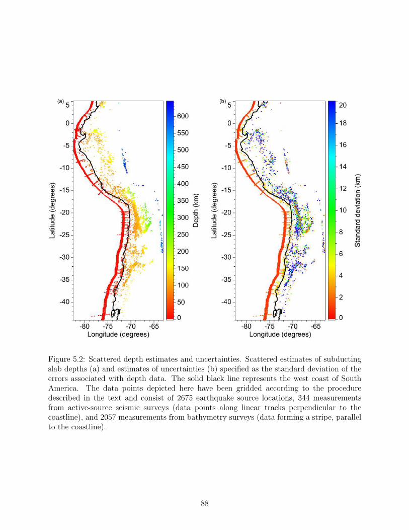
(a) (b)
Figure 5.2: Scattered depth estimates and uncertainties. Scattered estimates of subductingslab depths (a) and estimates of uncertainties (b) specified as the standard deviation of theerrors associated with depth data. The solid black line represents the west coast of SouthAmerica. The data points depicted here have been gridded according to the proceduredescribed in the text and consist of 2675 earthquake source locations, 344 measurementsfrom active-source seismic surveys (data points along linear tracks perpendicular to thecoastline), and 2057 measurements from bathymetry surveys (data forming a stripe, parallelto the coastline).
88

width (standard deviation σ) of the normal pdf is chosen based on the location uncertainty
reported in the earthquake catalog from which the data were extracted. For active seismic
and bathymetry data, the pdf half-width σ is based on an assumed uncertainty related to
time-to-depth conversion or estimates of sediment thickness (Hayes et al., 2012).
Secondary data consist of scattered estimates of the strike direction of the slab (Figure
5.3a). The strike data are taken (Hayes and Wald, 2009) from best-fitting double couples of
CMT solutions when available (using the gCMT catalog, www.globalcmt.org).
5.4.1 Initial gridding
As a first step, we use a uniform rectangular mesh with grid cells of size 0.1◦ × 0.1◦ to
grid the depth and strike data separately. The value assigned to each grid cell containing
bathymetry, active-source seismic, or strike data is the average of all sample values contained
in the cell. No values are assigned to the grid cells that contain no strike or depth data.
The depth value and the uncertainty assigned to a grid cell that contains more than
one earthquake sample are computed according to the weighted averaging scheme described
in Appendix F. This is because the uncertainties associated with earthquake depths are
variable and uncorrelated. Using this weighted averaging scheme ensures that more certain
depth estimates are given more weight in the averaging process than less certain estimates.
Figure 5.2a shows the location and values (depicted as colors) of the 5076 depth samples
after gridding, and Figure 5.2b shows the uncertainties associated with these samples on
a longitude-latitude map. The locations and values of the 458 gridded strike samples are
depicted in Figure 5.3a. The colors represent the estimates of the strike angle γ of the slab
measured relative to geographic north.
5.4.2 Interpolation of the strikes
To define the metric tensor field D using equations 5.1 and 5.2, we need the value of
the strike angle γ(u) at each grid point. Therefore, we must first interpolate the scattered
strikes.
89
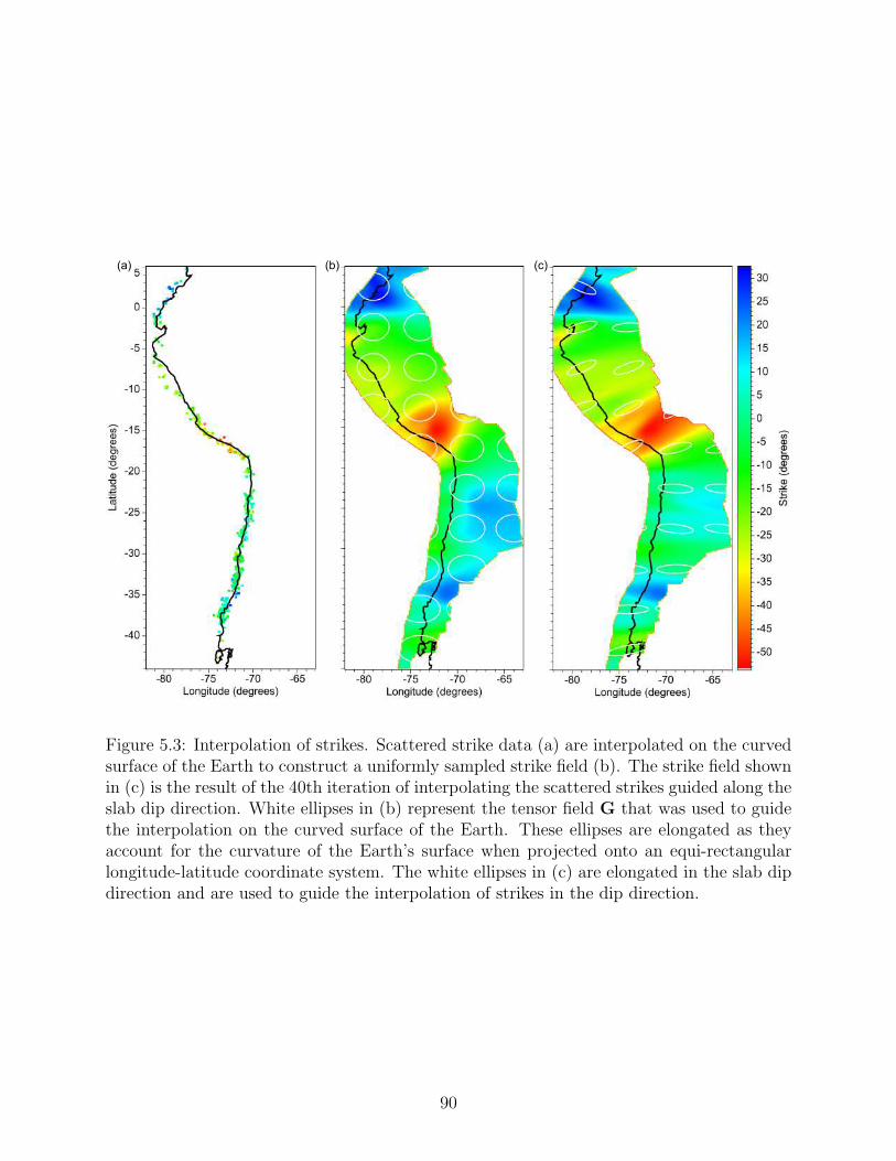
(b)(a) (c)
Figure 5.3: Interpolation of strikes. Scattered strike data (a) are interpolated on the curvedsurface of the Earth to construct a uniformly sampled strike field (b). The strike field shownin (c) is the result of the 40th iteration of interpolating the scattered strikes guided along theslab dip direction. White ellipses in (b) represent the tensor field G that was used to guidethe interpolation on the curved surface of the Earth. These ellipses are elongated as theyaccount for the curvature of the Earth’s surface when projected onto an equi-rectangularlongitude-latitude coordinate system. The white ellipses in (c) are elongated in the slab dipdirection and are used to guide the interpolation of strikes in the dip direction.
90

Strike data are only available in the region near the coastline (Figure 5.3a). This makes
it more difficult to produce accurate estimates of the strike angles for deeper parts of the
slab away from the coast. However, the strikes of the slab are most highly correlated in
the dip direction (perpendicular to the strike direction). This follows from the definition of
strike and dip for a dipping plane (Figure 5.1). Therefore, to obtain more accurate estimates
of the strike angles, we guide the interpolation of the scattered strikes in the dip direction
using an iterative scheme which consists of three steps:
(i) Interpolate the strikes using tensor-guided interpolation with a metric tensor field that
accounts for only the curved geometry of the Earth’s surface. In this case, the non-Euclidean
distances are simply geodesic. Therefore, we can use D = I in equation 5.8 to construct a
metric tensor field G defined as
G = F−1F−T . (5.10)
Figure 5.3b shows the result of the interpolation of scattered slab strikes as a uniformly
sampled strike field γg(u). The tensor field G used to guide this interpolation is represented
by the white ellipses.
(ii) Compute a dip direction field γd(u) using the strike field γg(u) as
γd(u) = γg(u) + 90◦ (5.11)
because the dip direction is perpendicular to the strike direction.
(iii) Construct a tensor field (white ellipses in Figure 5.3c) based on γd(u) and use it to
guide a new interpolation of scattered strikes in the dip direction. The result is a new strike
field we call γ(u).
This is the end of the first iteration. A new iteration starts by going back to step (ii) but
this time, instead of γg(u) in equation 5.11, we use γ(u) obtained in the previous iteration.
This process converges (after 40 iterations) to the strike field shown in Figure 5.3c.
91

(a) (b)
Figure 5.4: Two interpolations of slab depths. A strike-ignorant interpolation (a) of slabdepths on the Earth’s surface, in which the metric tensor field used to guide the interpolationof depths accounts for only the difference between Euclidean and geodesic distance and astrike-guided interpolation (b) in which the metric tensor field also accounts for estimatedstrike directions. Ellipses represent the metric tensor fields.
92
5.4.3 Interpolation of the depths
With the strike field γ(u) obtained above, we can now define the strike tensor field D
according to equations 5.2 and 5.3. Next, to account for the curvature of the Earth’s surface,
we modify D according to equation 5.8.
At this point we have all the components needed to perform a blended neighbor interpo-
lation of slab depths on the surface of the Earth. Figure 5.4 shows the results of two blended
neighbor interpolations of slab depths guided by two different tensor fields. In Figure 5.4a,
the tensor field G used to guide the interpolation (shown as white ellipses) accounts for
only the curvature of the Earth’s surface. In Figure 5.4b, the tensor field Du used to guide
the interpolation (shown as white ellipses) accounts for both that curvature and the strike
directions.
5.5 Cross-validation
The solution to any interpolation problem is non-unique and depends on the method used
for interpolation; the interpolants shown in Figure 5.4 are just two solutions among infinitely
many. These solutions were both obtained using the blended neighbor interpolation method.
However the metric tensor fields used to guide the interpolations were different.
A possible criterion for assessing the results of an interpolation method is to analyze the
accuracy of its predictions. We use a 10-fold cross-validation technique (Kohavi et al., 1995)
to find an optimal value for the parameter η in equation 5.3.
In 10-fold cross-validation, input samples are randomly partitioned into 10 mutually
exclusive subsets (the folds) of approximately equal size (Kohavi et al., 1995). Subsequently
10 iterations of interpolation and validation are performed such that within each iteration a
different subset of samples is held out for validation and the union of the remaining 9 subsets
(the training set) is used for interpolation.
The validation process involves computing the numerical difference between interpolated
values and test-set sample values normalized by the estimates of uncertainty (standard de-
93
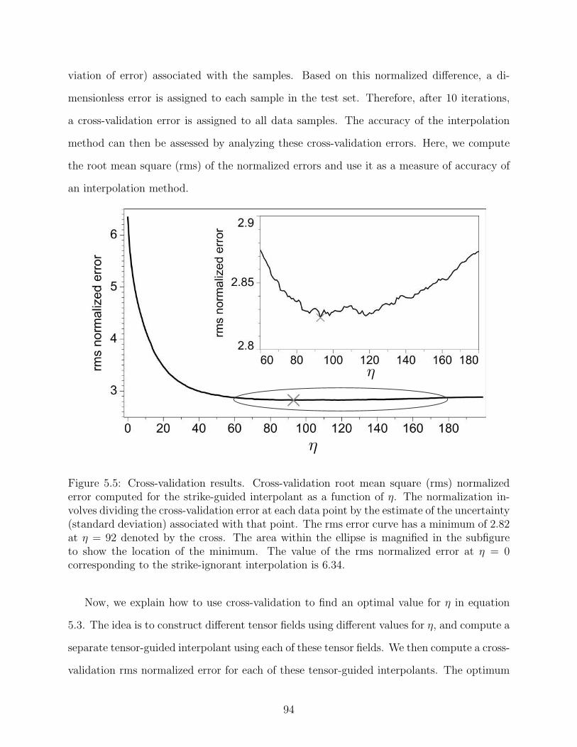
viation of error) associated with the samples. Based on this normalized difference, a di-
mensionless error is assigned to each sample in the test set. Therefore, after 10 iterations,
a cross-validation error is assigned to all data samples. The accuracy of the interpolation
method can then be assessed by analyzing these cross-validation errors. Here, we compute
the root mean square (rms) of the normalized errors and use it as a measure of accuracy of
an interpolation method.
η
η
Figure 5.5: Cross-validation results. Cross-validation root mean square (rms) normalizederror computed for the strike-guided interpolant as a function of η. The normalization in-volves dividing the cross-validation error at each data point by the estimate of the uncertainty(standard deviation) associated with that point. The rms error curve has a minimum of 2.82at η = 92 denoted by the cross. The area within the ellipse is magnified in the subfigureto show the location of the minimum. The value of the rms normalized error at η = 0corresponding to the strike-ignorant interpolation is 6.34.
Now, we explain how to use cross-validation to find an optimal value for η in equation
5.3. The idea is to construct different tensor fields using different values for η, and compute a
separate tensor-guided interpolant using each of these tensor fields. We then compute a cross-
validation rms normalized error for each of these tensor-guided interpolants. The optimum
94

value for η is the one corresponding to the interpolant with minimum cross-validation rms
normalized error.
One difficulty with this approach is that equation 5.3 requires knowledge of dip angles of
the slab. To compute the dip angles, we smooth the strike ignorant interpolant of Figure 5.4
in order to obtain an approximate initial slab model qi(u). Although inaccurate, this initial
model is good enough for the purpose of approximating dip angles as
δ(u) ≈ tan−1 ‖∇qi(u)‖. (5.12)
Substituting this approximation into equation 5.3 yields
λd(u) =1
1 + η‖∇qi(u)‖2 , (5.13)
which is more straightforward to implement than equation 5.3.
Figure 5.5 summarizes the results of the cross-validation process used to determine the
best choice for parameter η. The black curve shows the cross-validation rms normalized error
as a function of η. The most accurate strike-guided interpolant (the one with the minimum
cross-validation rms error) is obtained for η = 92.
For a quantitative comparison of the strike-ignorant and strike-guided interpolants shown
in Figure 5.4, we contrast their respective cross-validation rms normalized errors inferred
from the black curve in Figure 5.5. The rms normalized cross-validation error for strike-
guided interpolation with a tensor field constructed using η = 92 is approximately 2.82. The
same error for the strike-ignorant interpolation guided by a tensor field constructed using
η = 0 is more than three times larger, i.e., 6.34. The result of tensor-guided interpolation is
evidently more accurate.
5.6 Accounting for data uncertainties
The interpolant shown in Figure 5.4b matches all scattered input depth samples. This
is expected as the interpolation error must be (by definition) zero at the location of input
95
samples. However, for the reasons explained below, we assume that this interpolant surface
does not represent a geophysically reasonable model for the subduction interface, because the
surface is not smooth and contains abundant fluctuations. If real, such fluctuations would
imply unwarranted bending strains and stresses within the structure of the slab, especially in
the shallow parts where the slab is still relatively cold and brittle. Therefore, the fluctuations
observed in the interpolated depths are more likely the result of error in depth estimates and
do not represent the true geometry of the slab.
To account for errors in data in order to obtain a smoother model for the slab, we modify
the tensor-guided scheme presented above such that instead of interpolating the data it
results in a fitting solution. For this modification, we utilize the given estimates of data
uncertainties and incorporate them in a statistically plausible manner into the modeling
procedure.
5.6.1 From interpolation to data fitting
The tensor-guided procedure described so far is based on the blended neighbor interpola-
tion method (summarized in Appendix E). The first step of the blended neighbor method can
be interpreted as scattering the values fk corresponding to the nearest known sample points
xk to construct a nearest neighbor interpolant p(x). The second step of the blended neigh-
bor method can be interpreted as smoothing p(x) to obtain a blended neighbor interpolant
q(x). The extent of this smoothing at each location x is proportional to the non-Euclidean
distance t(x) from x to the nearest known sample (Hale, 2009). This means that at the loca-
tion of known samples, where t(x) = 0, no smoothing is applied so the solution to blending
equation E.4 is q(x) = p(x). Hence, the interpolation condition q(xk) = fk is satisfied and
the interpolant q(x) matches all scattered data.
Satisfying the interpolation condition is an implicit requirement of any interpolation
method. However, in situations where there is uncertainty associated with data, this con-
dition may not be desirable. In blended neighbor interpolation, the constraint of satisfying
the interpolation condition can be relaxed by adding a function w(x) to the term t2(x) in
96
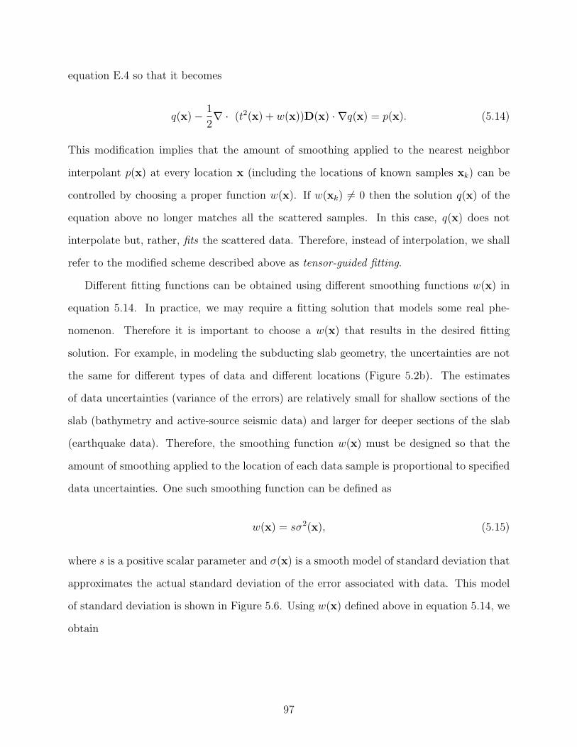
equation E.4 so that it becomes
q(x)− 1
2∇ · (t2(x) + w(x))D(x) · ∇q(x) = p(x). (5.14)
This modification implies that the amount of smoothing applied to the nearest neighbor
interpolant p(x) at every location x (including the locations of known samples xk) can be
controlled by choosing a proper function w(x). If w(xk) 6= 0 then the solution q(x) of the
equation above no longer matches all the scattered samples. In this case, q(x) does not
interpolate but, rather, fits the scattered data. Therefore, instead of interpolation, we shall
refer to the modified scheme described above as tensor-guided fitting.
Different fitting functions can be obtained using different smoothing functions w(x) in
equation 5.14. In practice, we may require a fitting solution that models some real phe-
nomenon. Therefore it is important to choose a w(x) that results in the desired fitting
solution. For example, in modeling the subducting slab geometry, the uncertainties are not
the same for different types of data and different locations (Figure 5.2b). The estimates
of data uncertainties (variance of the errors) are relatively small for shallow sections of the
slab (bathymetry and active-source seismic data) and larger for deeper sections of the slab
(earthquake data). Therefore, the smoothing function w(x) must be designed so that the
amount of smoothing applied to the location of each data sample is proportional to specified
data uncertainties. One such smoothing function can be defined as
w(x) = sσ2(x), (5.15)
where s is a positive scalar parameter and σ(x) is a smooth model of standard deviation that
approximates the actual standard deviation of the error associated with data. This model
of standard deviation is shown in Figure 5.6. Using w(x) defined above in equation 5.14, we
obtain
97

q(x)− 1
2∇ · (t2(x) + sσ2(x))D(x) · ∇q(x) = p(x). (5.16)
Here, parameter s controls the smoothness of the fitting solution q(x). Note that tensor-
guided interpolation is a special case (with s = 0) of the more general tensor-guided fitting
(with s > 0). The question left to be answered is, how to choose the smoothing parameter
s.
E
Figure 5.6: An approximate smooth model σ(x) of the standard deviation of the errorassociated with depth data. This model is used to design a spatially varying smoothingfunction.
98

5.6.2 Choosing the smoothing parameter
In real problems, constraints often make one fitting solution preferable to other possible
solutions. For instance, in constraining the geometry of a subduction slab, a geophysically
reasonable model for the slab is expected to be smooth. Nevertheless, such a model must
not be so smooth that sampled depths are completely disregarded. Therefore, to obtain an
optimum fitting function, we must find a balance between the smoothness of q(x) and the
degree to which it honors the information given by data. Before explaining how to find this
balance, we define some new terms.
We define the standardized data error (error in each depth sample value) as
ek =µk − fkσk
(5.17)
where k is the sample index, µk is the expected value of slab depth (true depth) at location
xk of the sample, fk is the sample value, and σk is the uncertainty or the standard deviation
of the error associated with the sample. Both µk and ek are unknown quantities.
Recall that each depth sample is assumed to be a random variable with a normal distribu-
tionN (µk, σk). Therefore, the standardized data error ek is expected to be a random variable
with standard normal distribution. From this, we infer that the collection of all standardized
data errors E, computed according to equation 5.17, also constitutes a population that is a
standard normal distribution, i.e.,
E ∼ N (0, 1). (5.18)
Similarly, we define the standardized fitting error (residual) at location xk of each sample
as
rk =q(xk)− fk
σk(5.19)
99

where k is the sample index, q(xk) is the value of the fitting function at location xk of the
sample, fk is the sample value, and σk is the uncertainty or standard deviation of the error
associated with the sample.
Our goal is to find a fitting function q(x) that correctly estimates the true slab depths.
If this goal is attained for some optimum fitting function qop(x), then we have qop(xk) = µk
and hence, by equations 5.17 and 5.19, rk = ek. This implies that, for the desired optimal
solution, the collection of all standardized fitting errors R will have a standard normal
distribution, i.e.,
R|qop(x) ∼ N (0, 1). (5.20)
This can be used as a criterion to choose the optimum smoothing parameter s in our
data-fitting method. In other words, we can analyze fitting errors associated with the fitting
solutions computed using different smoothing parameters, and then choose the one for which
R ∼ N (0, 1) as the optimal smoothing parameter s.
Note that our assumption about the normality of the distribution of the fitting errors
might not be accurate. Therefore, when assessing the distribution of the fitting errors, it is
important to use a robust statistic which is not severely affected by the potential outliers.
One such statistic is the interquartile range (IQR). ForN (0, 1), the IQR is the range of values
from -0.674 to 0.674 containing 50% of the population. Thus, for an optimum fitting solution,
half of the standardized fitting errors are expected to lie within the range [−0.674, 0.674].
To find the right smoothing parameter, we start from the interpolation solution (i.e.,
from s = 0) and then gradually increase the smoothness parameter until we reach a point
where half of the standardized fitting errors fall within and half fall outside of the IQR for
a standardized normal distribution. We choose the smoothing parameter s for which this
condition is satisfied to be the optimal fitting parameter and use it to compute the optimum
fitting solution.
100

AB B B
A B
Tensor-guided interpolation
Tensor-guided fitting
Slab1.0
(b) (d)(c)
(a)
A A
Figure 5.7: A cross section (a) showing the profiles of three different slab models. The slabmodel obtained by tensor-guided interpolation (b) is compared with the model obtained bytensor-guided fitting (c) and the same model from Slab1.0 (d) produced by Hayes et al.(2012). Line segment AB shows the geographical location of the vertical cross section shownin (a). The gray crosses in (a) are the orthogonal projection of all data points (the pointsshown in white in (b), (c), and (d)) that lie within a rectangular window of width 100 kmcentered on the vertical plane of section AB. The gray dots in (b), (c), and (d) denote thelocation of scattered data points.
101

5.7 Results and discussion
The final result of applying our tensor-guided fitting procedure to slab data is shown in
Figure 5.7c. Compared to the interpolating model (shown in Figure 5.7b), this fitting model
is smoother and is therefore likely to be more geophysically reasonable. The smoothing
parameter s = 0.56, employed in the tensor-guided fitting to produce the model in Figure
5.7c, was chosen using the method described in the previous section.
Figure 5.7d shows the Fitting solution known as Slab1.0 obtained by Hayes et al. (2012).
Slab1.0 is a 3D subduction geometry compilation of approximately 85% of the subduction
zones worldwide. Hayes and Wald (2009) and Hayes et al. (2012) used estimates of slab
strike derived from earthquake source mechanisms, depths of the earthquakes that those
mechanisms represent, and a collection of other complementary datasets to constrain the
geometry of the subduction interface. Their method fits the data with a 3D non-planar
surface interpolating between a series of 2D sections which sample the slab geometry every
10 km along the strike of the subduction zone. Each 2D section is constructed using Hermite
splines and consists of two parts: a polynomial fit of order 2 or 3 to shallow data (depth≤80
km) splined with a polynomial fit of order 3 or 4 to intermediate and deep data.
A cross-section profile of Slab1.0 is compared with the tensor-guided fitting and inter-
polating profiles in Figure 5.7a. In this cross section, the Slab1.0, the tensor-guided fitting,
and the tensor-guided interpolating profiles are the blue, red, and green curves, respec-
tively. Compared to the tensor-guided interpolation, the tensor-guided fitting profile is
clearly smoother. However, our fitting profile (red) is not as smooth as is the Slab1.0 profile
(blue). This is because Hayes et al. (2012) use low-degree polynomial splines to fit the data
in 2D sections. Therefore, Slab1.0 solution is forced to be smoother than the tensor-guided
fitting result in the cross section shown here. Nevertheless, our model honors the data more
precisely than the Slab1.0 model.
The tensor-guided fitting model is generally deeper than the Slab1.0 model and the
difference between the two models is in most areas between 0 and 40 km. This difference
102
is partly due to the fact that, unlike shallow earthquakes, deep earthquakes (depth>80 km)
occur within the slab, not at its interface (Hayes et al., 2009). To account for the occurrence
of deep earthquakes within the slab, the method used to produce Slab1.0 involves an extra
step of shifting the deep seismicity 10 km horizontally in a direction farther from the trench.
These horizontal shifts are somewhat arbitrary (Hayes et al., 2009). The tensor-guided
process used to generate the surface shown in Figure 5.7c, however, does not include this
extra step to account for the displacement of deep hypocenters relative to the slab interface.
In this respect, the surface in Figure 5.7c represents not the slab interface, but the average
(most likely) locus of the hypocenter of the subduction-related earthquakes.
If a model describing the average depth of the seismicity beneath the slab interface (e.g.,
estimates of vertical distance from the slab interface to the hypocenters as a function of
longitude and latitude) is available, then it can be used to modify the depths in our tensor-
guided fitting surface (Figure 5.7c) in order to obtain a model for the slab interface. The
model required for this modification can be inferred, for example, from receiver functions or
tomographic studies such as Phillips et al. (2012) and Tonegawa et al. (2005).
Results of numerical tests, not shown here, indicate that tensor-guided fitting closely
approximates a linear process with respect to the vertical (depth) coordinate. In other
words, the surface obtained by tensor-guided fitting (Figure 5.7c) is nearly a linear func-
tion of the slab depths being fitted. Therefore, any modification like that described above
can be applied either to scattered depths before fitting, or to a surface (Figure 5.7c) after
fitting. Consequently, our tensor-guided fitting process can be applied without regard for
such modifications, which will vary depending on which model is chosen for displacements
of earthquake hypocenters relative to slab interfaces.
The tensor-guided fitting and interpolating solutions change concavity with their slopes
approaching horizontal at the eastern edge of the model (see Figure 5.7a around distance
750-900 km and depth 350-500 km). This is due to the use of a zero-slope boundary condition
in solving the system of partial differential equations 5.16.
103
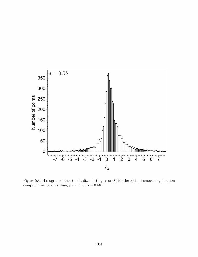
rk
a) s=0
s = 0.56
Figure 5.8: Histogram of the standardized fitting errors rk for the optimal smoothing functioncomputed using smoothing parameter s = 0.56.
104
Figure 5.8 shows the histogram of standardized fitting errors rk associated with the
optimum fitting solution computed using smoothing parameter s = 0.56. Note that this
histogram does not represent a normal distribution (the long tails of the distribution observed
here are not expected for a normal distribution), which suggests that the normal distribution
assumed to describe the data errors is not accurate and therefore, this study might benefit
from assuming a different type of distribution (e.g., double exponential) for the data and
fitting errors. Also, note that the histogram in Figure 5.8 is not centered at 0, which indicates
a bias towards positive fitting errors. As explained below, the observed bias is a consequence
of the geometry of the problem, and the smoothing applied in our fitting procedure.
The slab geometry is almost horizontal in areas near the coastline. Therefore, the tensors
used in the tensor-guided fitting procedure in these areas have low eccentricity (e.g., see the
nearly circular ellipses to the left of the coastline in Figure 5.4). One consequence of using
these tensors in the smoothing step is that the fitting solution q(x) in the bathymetry area
receives contribution from the deeper sections of the slab. Thus, q(xk) is more likely to
overestimate the slab depth at locations xk of the bathymetry samples. This means that
the standardized fitting errors defined in equation 5.19 are more likely to be positive than
negative for the bathymetry data. Recall that about 40% of the depth samples in this study
are bathymetry data, which are densely clustered near the coastline (Figure 5.2). Therefore,
the positive fitting errors statistically outnumber the negative fitting errors and a positive
bias in the distribution of errors is created.
5.8 Conclusion
Additional information provided by spatially scattered and sparsely sampled secondary
data can be used to guide the interpolation or fitting of spatially scattered primary data.
Through the example of modeling the geometry of a subducting slab interface, we demon-
strated the construction of a metric tensor field that defines an anisotropic and spatially
varying correlation model for primary data. We showed that this metric tensor field can be
readily modified to account for the non-Euclidean distances between data points that are
105
acquired on the non-planar (spherical) surface of the Earth.
Proper handling of data uncertainties is an important aspect of data-fitting methods. If
estimates of uncertainties associated with data are available, they can be easily incorporated
into the tensor-guided fitting procedure described in this paper to produce a statistically
consistent fit to the scattered data. We used slab data (estimates of depths and uncertainties
in depth measurements) to demonstrate the capability of our data-fitting method in handling
data uncertainties.
Our method relies on the statistical model that describes errors in data. Therefore,
assuming a more accurate statistic model for the data uncertainties would improve the
results of our method.
5.9 Data and resources
All data used in this paper came from published sources listed in the references. The
software used to produce the results was written in Java with the use of libraries in the Mines
Java Toolkit (http://inside.mines.edu/~dhale/jtk/index.html) last accessed Septem-
ber 24 2014.
5.10 Acknowledgments
We wish to thank Simon Luo for the helpful discussions on this paper and Diane Witters
for her instructions on revision and editing. We also thank William Barnhart, USGS, and
two anonymous BSSA reviewers, for detailed comments that helped improve the manuscript.
This research was supported by the sponsors of the Center for Wave Phenomena at the
Colorado School of Mines.
106
CHAPTER 6
SUMMARY
In this thesis, I introduce a new method for optimal imaging of a seismic source in a
medium with known properties using an arbitrary receiver array. To work properly, time-
reversal-based source-imaging methods require full-aperture receiver arrays that allow ade-
quate sampling of the original source wavefield. When acquisition is incomplete, the ability
of the time-reversal (TR) methods to reconstruct the source wavefield and properly image the
source is compromised. The Backus-Gilbert (BG) source-imaging method is designed specif-
ically to address this problem by optimally focusing the wavefield onto the source position
in an experiment with a given source-receiver configuration.
6.1 General conclusions
The theoretical foundation of the BG method is formulated in Chapter 2, where acoustic
wave focusing is cast as an optimization problem in the style of the Backus-Gilbert method
in geophysical inverse theory. The new approach presented in Chapter 2 enhances the spatial
resolution of the TR focusing process by tailoring the back-projected signals in amplitude
and shape to achieve an optimally sharp focus at a desired point in space. The property of
source-receiver reciprocity in the acoustic Green function allows the theory of BG focusing
to be reinterpreted and used as an imaging algorithm to image a point source with an
impulsive time function originated from an unknown point in space. The linearity of the
source-imaging problem is then used to extend the BG method for imaging sources with
finite spatial dimension and with arbitrary time dependence.
I further generalize the theory of BG source imaging for elastic waves in Chapter 3. By
reproducing the source radiation pattern, the BG method is capable of retrieving the source
mechanism. As in the acoustic case, the elastic BG method ultimately boils down to a linear
system of equations that must be formed and solved separately for each frequency component
107
in data. Apart from acquiring the data in the field, constructing these linear systems requires
two pieces of information: an estimate of source location and a model describing the elastic
(or acoustic) properties of the medium. The best BG images are obtained when the size of
the monitoring area (the optimization window known to contain the source) is about 2-3
times the dominant P-wavelength. The properties of the medium (earth model) are needed
by BG for computing the elastodynamic Green tensor for each receiver location. These
Green tensors must ideally be precise. Nevertheless, numerical experiments shown in this
thesis (Chapters 2 and 4) indicate that the BG method offers a better-resolved image of the
source than TR does, even when the earth model is inaccurate.
Computing the Green tensor for each receiver is the most computationally demanding
step in the BG process. However, for earthquake or reservoir monitoring systems with
permanent stations, the Green tensors can be computed and stored a-priori and need not be
computed more than once. In other words, the matrix in the BG linear system can be formed
and inverted once and then reused for imaging all subsequent earthquakes. Pre-computing
and storing the Green tensors can significantly improve the computational efficiency of the
BG method and make it comparable in cost to TR imaging. Surface microseismic surveys
could involve thousands of receivers. In such situations, computing the Green tensor for all
receiver locations may not be practical. To address this practical issue, in Appendix B, I
introduce a time-domain version of the BG method which does not require computation of
the Green tensors. Solving the BG optimization problem in the time domain involves an
iterative solution, where each iteration includes two wave-propagation steps.
In Chapter 4, I formulate source imaging as an underdetermined linear inverse problem.
Analysing the BG method in the context of linear inverse theory facilitates the interpretation
sensitivity tests discussed later in Chapter 4. Numerical tests examining the stability of the
BG method indicate that, if properly regularized, the Backus-Gilbert method can tolerate
the presence of noise in data with signal-to-noise ratio as low as 1.
108
Chapter 5 presents a data-fitting method for constructing a model for the subducting
slab interface in South America. The method takes two sets of data as input. The primary
data used by the fitting method are the slab depth samples which are inferred from the
source location of the earthquakes that occur on or within the slab. The secondary data
used by the method are estimates of slab strikes inferred from the focal mechanism of the
subduction-related earthquakes. These scattered strike samples are used to infer a model
for spatial correlation that guides a blended neighbor interpolation of the depth of the slab
as a function of the horizontal coordinates. The fitting method also takes into account the
uncertainty associated with the depth measurements such that the constructed slab model
is statistically consistent with the given uncertainties. The accuracy of the constructed slab
model depends on the accuracy of the input data, i.e., scattered depth and strike estimates.
Using BG for source imaging can lead to better estimates of source location and more precise
determination of the focal mechanism of earthquakes, especially those in poorly instrumented
areas. One nice feature of the source-imaging methods, e.g., TR or BG, is that the extent
of the source image (focal spot) readily provides an estimate for the uncertainty in source
location (Gajewski and Tessmer, 2005).
6.2 Future research
The research presented in this dissertation can be extended in several intriguing theo-
retical and applied directions. Three possible directions for follow-up research are suggested
below.
6.2.1 L1-norm optimization
In Chapter 4, I showed that the solution which BG provides for the under-determined
source-imaging problem dn×1 = Gn×m mm×1, n < m is equivalent to the answer that one
would obtain by solving the optimization program min ‖m‖2 s.t. ‖d −Gm‖2 ≤ ε. This
solution is simplest among many possible solutions that could explain the data. Here, what is
meant by the simplest solution is the solution with the smallest L2-norm. The use of L2-norm
109

as a measure of simplicity for the solution of this optimization problem is somewhat arbitrary.
One possible alternative is to use the sparsity-promoting L1-norm for this purpose (Aster
et al., 2013). That is, instead of the above program, solvemin‖m‖1s.t.‖d−Gm‖2 ≤ ε. Using
the L1-norm in the formulation of the source-characterization or imaging problem is deemed
desirable because finding a sparse solution can lead to a better localization of the source or a
more focused source image. The drawback is that solving an optimization problem involving
L1-norm is generally more complicated compared to the corresponding L2-norm problem.
This is because L1-norm does not lead to a linear system of equations. Further research is
required to understand the feasibility and possible advantages of formulating source imaging
as an L1-norm optimization problem.
6.2.2 Super-resolution
The BG method is designed to optimize the resolution of the TR imaging by mitigating
the effects of incomplete acquisition. However, apart from acquisition geometry, the resolving
power of the TR process also depends on the bandwidth of the recorded seismograms and is
bounded by the diffraction limit. That is, a TR image of a point source, even with complete
acquisition, is a spot (Airy disk) that cannot be smaller than half a wavelength. The reason
for this is that sub-wavelength information about the source is carried by exponentially
decaying evanescent waves that never reach the receivers in the far-field (Lerosey et al.,
2007). Therefore, because the TR process cannot regenerate these lost evanescent waves in
the back-propagation step, it cannot focus waves beyond the diffraction limit.
Most techniques for improving the resolution of imaging beyond the diffraction limit in-
volve regeneration of the evanescent waves required for subwavelength focusing (e.g., Schuster
et al., 2012; Fink, 2008). These methods often take advantage of the presence of a scatterer
in the near-field region of the focusing target. Alternatively, de Rosny and Fink (2002)
showed that, to be complete, a TR process must ideally involve a sink (time-reversed source)
in the back-propagation step so that the forward- and back-propagation steps are exactly
symmetric in time. They showed experimentally that it is possible to beat the diffraction
110
limit if the back propagation step of the TR process is modified by introducing a sink at
the initial source location. However, careful theoretical analysis of this modified TR process
reveals that introducing the sink indirectly implies the regeneration of the evanescent waves
in the back-propagation step. Note that to use this trick, i.e., to fix the TR process by
adding a sink, one needs to know the source.
A completely different approach to super-resolution was originated in the super-directive
antenna theory in the microwave community (Schelkunoff, 1943). A super-directive antenna
is a finite-size antenna array that is capable of radiating an arbitrarily sharp beam by tai-
loring the waves emitted by each array element (Wong and Eleftheriades, 2010; Rogers and
Zheludev, 2013). Using concepts of super-directive antennas in diffraction optics, Toraldo
Di Francia (1952) showed that super-resolution can be achieved locally with no need for
evanescent waves. The caveat is that the power delivered to the target spot is only a fraction
of the total power input to the system. Most of the energy goes to the sidebands in the focus
plane outside a silent area designed around the main focal spot.
In many respects, an array of receivers in acoustics (or in seismology) resemble an antenna
or an optical imaging device. The problem of improving the resolving power of an array of
receivers is also common to these disciplines. One interesting question is whether the BG
formalism is capable of beating the diffraction limit. Answering this question needs more
research.
6.2.3 Underwater acoustics
One application of TR focusing is in underwater acoustics (Jackson and Dowling, 1991;
Kuperman et al., 1998; Hodgkiss et al., 1999; Edelmann et al., 2002). As in any TR applica-
tion, the limited aperture of the receiver array can have a negative effect on the performance
of TR in underwater acoustics problems. However, two specific properties of underwater
acoustics problems make them particularly suitable for application of the BG method. First,
recall that one of the main requirements of the BG method is accurate knowledge of the prop-
agating medium. The propagation velocity of the acoustic waves in water can be estimated
111

with relatively high precision. Second, as shown in Chapter 2, BG can use reflection events
in data to augment the illumination of the target and significantly improve the quality of
the focus or the source image. In underwater acoustics experiments, the multiply reflected
waves in the water layer are recorded by the receivers as strong events in data. The above
properties make underwater acoustics a promising area for application of the BG method.
Obviously, there are specific complications, such as the temporal variability of the sea level
and water velocity, that must be considered and carefully addressed.
112

REFERENCES CITED
Aki, K., and P. Richards, 1980, Quantitative seismology theory and methods, vol. 2: Freemanand Company.
——–, 2002, Quantitative seismology 2nd edition: University Science Books.
Artman, B., I. Podladtchikov, and B. Witten, 2010, Source location using time-reverse imag-ing: Geophysical Prospecting, 58, 861–873.
Aster, R. C., B. Borchers, and C. H. Thurber, 2013, Parameter estimation and inverseproblems: Academic Press.
Aubry, J.-F., M. Tanter, J. Gerber, J.-L. Thomas, and M. Fink, 2001, Optimal focusing byspatio-temporal inverse filter. ii. experiments. application to focusing through absorbingand reverberating media: The Journal of the Acoustical Society of America, 110, 48–58.
Backus, G., and F. Gilbert, 1968, The resolving power of gross earth data: GeophysicalJournal International, 16, 169–205.
——–, 1970, Uniqueness in the inversion of inaccurate gross earth data: Philosophical Trans-actions for the Royal Society of London. Series A, Mathematical and Physical Sciences,266, 123–192.
Backus, G., and J. Gilbert, 1967, Numerical applications of a formalism for geophysicalinverse problems: Geophysical Journal International, 13, 247–276.
Baig, A., and T. Urbancic, 2010, Microseismic moment tensors: A path to understandingfrac growth: The Leading Edge, 29, 320–324.
Berkhout, A., 1997, Pushing the limits of seismic imaging, part i: Prestack migration interms of double dynamic focusing: Geophysics, 62, 937–953.
Bevis, M., and B. L. Isacks, 1984, Hypocentral trend surface analysis: Probing the geometryof benioff zones: Journal of Geophysical Research: Solid Earth (1978–2012), 89, 6153–6170.
Blomgren, P., G. Papanicolaou, and H. Zhao, 2002, Super-resolution in time-reversal acous-tics: The Journal of the Acoustical Society of America, 111, 230–248.
113

Boisvert, J., J. Manchuk, and C. Deutsch, 2009, Kriging in the presence of locally varyinganisotropy using non-Euclidean distances: Mathematical Geosciences, 41, 585–601.
Born, M., and E. Wolf, 1999, Principles of optics: electromagnetic theory of propagation,interference and diffraction of light: CUP Archive.
Briggs, I. C., 1974, Machine contouring using minimum curvature: Geophysics, 39, 39–48.
Broggini, F., R. Snieder, and K. Wapenaar, 2012, Focusing the wavefield inside an unknown1d medium: Beyond seismic interferometry: Geophysics, 77, A25–A28.
Cassereau, D., and M. Fink, 1993, Focusing with plane time-reversal mirrors: An efficientalternative to closed cavities: The Journal of the Acoustical Society of America, 94, 2373–2386.
Claerbout, J. F., and I. Green, 2008, Basic earth imaging: Citeseer.
Curriero, F. C., 2006, On the use of non-Euclidean distance measures in geostatistics: Math-ematical Geology, 38, 907–926.
de Rosny, J., and M. Fink, 2002, Overcoming the diffraction limit in wave physics using atime-reversal mirror and a novel acoustic sink: Physical review letters, 89, 124301.
Eaton, D. W., and F. Forouhideh, 2011, Solid angles and the impact of receiver-array geom-etry on microseismic moment-tensor inversion: Geophysics, 76, WC77–WC85.
Edelmann, G. F., T. Akal, W. S. Hodgkiss, S. Kim, W. A. Kuperman, and H. C. Song,2002, An initial demonstration of underwater acoustic communication using time reversal:Oceanic Engineering, IEEE Journal of, 27, 602–609.
Eisner, L., S. Williams-Stroud, A. Hill, P. Duncan, and M. Thornton, 2010, Beyond the dotsin the box: Microseismicity-constrained fracture models for reservoir simulation: TheLeading Edge, 29, 326–333.
Fink, M., 1997, Time reversed acoustics: Physics today, 50 (3), 34–40.
——–, 2006, Time-reversal acoustics in complex environments: Geophysics, 71, SI151–SI164.
——–, 2008, Time-reversal waves and super resolution: Journal of Physics: ConferenceSeries, IOP Publishing, 012004.
Fink, M., and M. Tanter, 2010, Multiwave imaging and super resolution: Physics Today, 63(2), 28–33.
114

Gajewski, D., and E. Tessmer, 2005, Reverse modelling for seismic event characterization:Geophysical Journal International, 163, 276–284.
Gaspar, C., 1999, Multigrid technique for biharmonic interpolation with application to dualand multiple reciprocity method: Numerical Algorithms, 21, 165–183.
Gudmundsson, O., and M. Sambridge, 1998, A regionalized upper mantle (rum) seismicmodel: Journal of Geophysical Research: Solid Earth (1978–2012), 103, 7121–7136.
Haddadin, O. S., and E. S. Ebbini, 1998, Ultrasonic focusing through inhomogeneous mediaby application of the inverse scattering problem: The Journal of the Acoustical Society ofAmerica, 104, 313–325.
Hale, D., 2009, Image-guided blended neighbor interpolation of scattered data: SEG, Ex-panded Abstracts, 28, 1127–1131.
——–, 2010, Image-guided 3D interpolation of borehole data: SEG, Expanded Abstracts,29, 1266–1270.
——–, 2011, Tensor-guided interpolation on non-planar surfaces: Technical Report CWP-696, Center for Wave Phenomena, Colorado School of Mines.
Hayes, G. P., and D. J. Wald, 2009, Developing framework to constrain the geometry ofthe seismic rupture plane on subduction interfaces a priori–a probabilistic approach: Geo-physical Journal International, 176, 951–964.
Hayes, G. P., D. J. Wald, and R. L. Johnson, 2012, Slab1.0: A three-dimensional model ofglobal subduction zone geometries: Journal of Geophysical Research, 117, 1–15.
Hayes, G. P., D. J. Wald, and K. Keranen, 2009, Advancing techniques to constrain thegeometry of the seismic rupture plane on subduction interfaces a priori: Higher-orderfunctional fits: Geochemistry, Geophysics, Geosystems, 10, 1–19.
Hodgkiss, W., H. C. Song, W. Kuperman, T. Akal, C. Ferla, and D. Jackson, 1999, A long-range and variable focus phase-conjugation experiment in shallow water: The Journal ofthe Acoustical Society of America, 105, 1597–1604.
Hyndman, R., M. Yamano, and D. Oleskevich, 1997, The seismogenic zone of subductionthrust faults: Island Arc, 6, 244–260.
Isaaks, E. H., and R. M. Srivastava, 1989, An introduction to applied geostatistics: Oxforduniversity press.
115

Jackson, D. D., 1979, The use of a priori data to resolve non-uniqueness in linear inversion:Geophysical Journal International, 57, 137–157.
Jackson, D. R., and D. R. Dowling, 1991, Phase conjugation in underwater acoustics: TheJournal of the Acoustical Society of America, 89, 171–181.
Jost, M. u., and R. Herrmann, 1989, A students guide to and review of moment tensors:Seismological Research Letters, 60, 37–57.
Kawakatsu, H., P. Kumar, Y. Takei, M. Shinohara, T. Kanazawa, E. Araki, and K. Suyehiro,2009, Seismic evidence for sharp lithosphere-asthenosphere boundaries of oceanic plates:Science, 324, 499–502.
Kawakatsu, H., and J.-P. Montagner, 2008, Time-reversal seismic-source imaging andmoment-tensor inversion: Geophysical Journal International, 175, 686–688.
Kim, Y., Q. Liu, and J. Tromp, 2011, Adjoint centroid-moment tensor inversions: Geophys-ical Journal International, 186, 264–278.
Kohavi, R., et al., 1995, A study of cross-validation and bootstrap for accuracy estimationand model selection: International Joint Conference on Artificial Intelligence (IJCAI),20-25 August 1995, Morgan Kaufmann, Montreal, Quebec, Canada, 1137–1145.
Kuperman, W., W. S. Hodgkiss, H. C. Song, T. Akal, C. Ferla, and D. R. Jackson, 1998,Phase conjugation in the ocean: Experimental demonstration of an acoustic time-reversalmirror: The journal of the Acoustical Society of America, 103, 25–40.
Larmat, C., R. Guyer, and P. Johnson, 2009, Tremor source location using time reversal:Selecting the appropriate imaging field: Geophysical Research Letters, 36, 22304.
Larmat, C., R. A. Guyer, and P. A. Johnson, 2010, Time-reversal methods in geophysics:Phys. Today, 63 (8), 31–35.
Larmat, C., J.-P. Montagner, M. Fink, Y. Capdeville, A. Tourin, and E. Clevede, 2006,Time-reversal imaging of seismic sources and application to the great sumatra earthquake:Geophysical Research Letters, 33, L19312.
Lerosey, G., J. de Rosny, A. Tourin, and M. Fink, 2007, Focusing beyond the diffractionlimit with far-field time reversal: Science, 315, 1120–1122.
Lokmer, I., G. S. O’Brien, D. Stich, and C. J. Bean, 2009, Time reversal imaging of syntheticvolcanic tremor sources: Geophysical Research Letters, 36, L12308.
116

Lu, R., et al., 2008a, Time reversed acoustics and applications to earthquake location andsalt dome flank imaging: PhD thesis, Massachusetts Institute of Technology.
Lu, R., M. N. Toksoz, M. E. Willis, et al., 2008b, Locating microseismic events with timereversed acoustics: a synthetic case study: 2008 SEG Annual Meeting, Society of Explo-ration Geophysicists, 1342–1346.
Maxwell, S. C., and T. I. Urbancic, 2001, The role of passive microseismic monitoring in theinstrumented oil field: The Leading Edge, 20, 636–639.
McMechan, G. A., 1982, Determination of source parameters by wavefield extrapolation:Geophysical Journal International, 71, 613–628.
——–, 1983, Migration by extrapolation of time-dependent boundary values: GeophysicalProspecting, 31, 413–420.
McMechan, G. A., J. Luetgert, and W. Mooney, 1985, Imaging of earthquake sources inlong valley caldera, california, 1983: Bulletin of the Seismological Society of America, 75,1005–1020.
Menke, W., 2012, Geophysical data analysis: discrete inverse theory: Academic press.
Montaldo, G., M. Tanter, and M. Fink, 2003, Real time inverse filter focusing throughiterative time reversal: The Journal of the Acoustical Society of America, 115, 768–775.
Nemeth, T., C. Wu, and G. T. Schuster, 1999, Least-squares migration of incomplete reflec-tion data: Geophysics, 64, 208–221.
Parker, R. L., 1994, Geophysical inverse theory: Princeton university press.
Parvulescu, A., 1961, Signal detection in a multipath medium by MESS processing: TheJournal of the Acoustical Society of America, 33, 1674–1674.
Phillips, K., R. W. Clayton, P. Davis, H. Tavera, R. Guy, S. Skinner, I. Stubailo, L. Audin,and V. Aguilar, 2012, Structure of the subduction system in southern peru from seismicarray data: Journal of Geophysical Research, 117, B11306.
Rentsch, S., S. Buske, S. Luth, and S. Shapiro, 2006, Fast location of seismicity: A migration-type approach with application to hydraulic-fracturing data: Geophysics, 72, S33–S40.
Robert, J.-L., and M. Fink, 2008, Greens function estimation in speckle using the decom-position of the time reversal operator: Application to aberration correction in medicalimaging: The Journal of the Acoustical Society of America, 123, 866–877.
117
Rogers, E. T., and N. I. Zheludev, 2013, Optical super-oscillations: sub-wavelength lightfocusing and super-resolution imaging: Journal of Optics, 15, 094008.
Schelkunoff, S. A., 1943, A mathematical theory of linear arrays: Bell System TechnicalJournal, 22, 80–107.
Schuster, G. T., et al., 2002, Reverse-time migration= generalized diffraction stack migration:SEG Technical Program Expanded Abstracts, 1280–1283.
Schuster, G. T., S. Hanafy, and Y. Huang, 2012, Theory and feasibility tests for a seismicscanning tunnelling macroscope: Geophysical Journal International, 190, 1593–1606.
Shapiro, S. A., 2008, Microseismicity a tool for reservoir characterization: EAGE Publica-tions bv.
Shearer, P. M., 2009, Introduction to seismology: Cambridge University Press.
Snieder, R., 2002, Time-reversal invariance and the relation between wave chaos and classicalchaos, in Imaging of complex media with acoustic and seismic waves: Springer, 1–16.
——–, 2004, A guided tour of mathematical methods for the physical sciences, 2nd ed.:Cambridge University Press.
Snieder, R., and J. Trampert, 1999, Inverse problems in geophysics, in Wavefield inversion:Springer Verlag, 119–190.
Song, F., and M. N. Toksoz, 2011, Full-waveform based complete moment tensor inver-sion and source parameter estimation from downhole microseismic data for hydrofracturemonitoring: Geophysics, 76, WC103–WC116.
Stein, S., and M. Wysession, 2003, An introduction to seismology, earthquakes, and earthstructure: Blackwell publishing.
——–, 2009, An introduction to seismology, earthquakes, and earth structure: John Wiley& Sons.
Steiner, B., E. H. Saenger, and S. M. Schmalholz, 2008, Time reverse modeling of low-frequency microtremors: Application to hydrocarbon reservoir localization: GeophysicalResearch Letters, 35, L03307.
Syracuse, E. M., and G. A. Abers, 2006, Global compilation of variations in slab depth be-neath arc volcanoes and implications: Geochemistry, Geophysics, Geosystems, 7, Q05017.
118

Tanter, M., J. Aubry, J. Gerber, J. Thomas, and M. Fink, 2001, Optimal focusing byspatio-temporal inverse filter. i. basic principles.: The Journal of the Acoustical Society ofAmerica, 110, 37–47.
Tanter, M., J.-L. Thomas, and M. Fink, 2000, Time reversal and the inverse filter: TheJournal of the Acoustical Society of America, 108, 223–234.
Tarantola, A., 2005, Inverse problem theory and methods for model parameter estimation:SIAM.
Tonegawa, T., K. Hirahara, and T. Shibutani, 2005, Detailed structure of the upper mantlediscontinuities around the japan subduction zone imaged by receiver function analyses:Earth, Planets, and Space, 57, 5–14.
Toraldo Di Francia, G., 1952, Super-gain antennas and optical resolving power: Il NuovoCimento (1943-1954), 9, 426–438.
Ulrich, T., B. Anderson, P.-Y. Le Bas, C. Payan, J. Douma, and R. Snieder, 2012, Improvingtime reversal focusing through deconvolution: 20 questions: Proceedings of Meetings onAcoustics, Acoustical Society of America, 045015.
Vellekoop, I., A. Lagendijk, and A. Mosk, 2010, Exploiting disorder for perfect focusing:Nature Photonics, 4, 320–322.
Wang, K., and J. He, 2008, Effects of frictional behavior and geometry of subduction faulton coseismic seafloor deformation: Bulletin of the Seismological Society of America, 98,571–579.
Wapenaar, K., F. Broggini, and R. Snieder, 2012, Creating a virtual source inside a mediumfrom reflection data: heuristic derivation and stationary-phase analysis: Geophysical Jour-nal International, 190, 1020–1024.
Weber, O., Y. S. Devir, A. M. Bronstein, M. M. Bronstein, and R. Kimmel, 2008, Parallelalgorithms for approximation of distance maps on parametric surfaces: ACM Transactionson Graphics (TOG), 27 (4), 1–25.
Wessel, P., 2009, A general-purpose green’s function-based interpolator: Computers & Geo-sciences, 35, 1247–1254.
Wong, A. M., and G. V. Eleftheriades, 2010, Adaptation of schelkunoff’s superdirective an-tenna theory for the realization of superoscillatory antenna arrays: Antennas and WirelessPropagation Letters, IEEE, 9, 315–318.
119

Wu, R.-S., and A. Ben-Menahem, 1985, The elastodynamic near field: Geophysical JournalInternational, 81, 609–621.
Xuan, R., and P. Sava, 2010, Probabilistic microearthquake location for reservoir monitoring:Geophysics, 75, MA9–MA26.
Zhu, T., 2014, Time-reverse modelling of acoustic wave propagation in attenuating media:Geophysical Journal International, 197, 1–12.
120
APPENDIX A - OPTIMIZED IMAGING OF AN EXTENDED ACOUSTIC SOURCE
In section 2.5, we discussed application of acoustic the BG method for imaging an im-
pulsive source at an unknown time and location. Here, we show that this method is equally
applicable for imaging any source function (not just impulsive) with an arbitrary spatio-
temporal characteristic. Let s(x, t) denote the spatio-temporal source function defined over
all space and time such that it can be nonzero only for x ∈ W and t ∈ [0, T ]. We can think
of the source function as a succession of spatially impulsive sources that are applied with
strength s(ξ, t) at each location ξ and write
s(x, t) =
∫s(ξ, t) δ(x− ξ) dξ . (A.1)
The data recorded by a station at xi associated with this distribution of impulsive sources
can then be written as
di(t) =
∫s(ξ, t) ∗G(xi, t; ξ, 0) dξ , (A.2)
where G(xi, t; ξ, τ) is the Green function with the source at x = ξ. In the frequency domain,
equation A.2 becomes
di(ω) =
∫s(ξ, ω)G(xi; ξ, ω) dξ . (A.3)
Having defined the source function and the data associated with it, we can now lay out
the BG optimization problem.
We assume that the scalar source wavefield at the time of focus is proportional to the
source function s(x, t), with unity as the proportionality constant. With this assumption,
we define our goal as finding signals ai(t) such that the difference between the wavefield
φ(x, t) = ai(t) ∗G(x, t; xi, 0) and the time-reversed source fucntion s(x, T − t) is minimum.
121

This can be achieved by minimizing an objective function defined as
J =
∫∫W
|φ(x, t)− s(x, T − t)|2dx dt, (A.4)
which can be expressed in the frequency domain as
J(ω) =
∫W
∣∣∣∣ ai(ω)G(x; xi, ω)−∫eiωT s∗(ξ, ω) δ(x− ξ) dξ
∣∣∣∣2 dx, (A.5)
for each frequency. Minimization A.5 with respect to ai(ω) gives
aj(ω)
∫W
G(x; xi, ω)G∗(x; xj, ω)dx
= eiωT∫s∗(ξ, ω)G∗(ξ; xi, ω) dξ
= eiωT∫s∗(ξ, ω)G∗(xi; ξ, ω) dξ ,
(A.6)
where in the last step we have used the reciprocity principle for the acoustic Green function.
Using equation A.3, equation A.6 can be written as
aj(ω)
∫W
G(x; xi, ω)G∗(x; xj, ω) dx = eiωT di∗(ω) , (A.7)
or more concisely
Γ(ω) a(ω) = eiωTd∗(ω) , (A.8)
where Γ is an N ×N matrix with the same definition as given by equation 2.5 in section 2.3
and d(ω) is an N ×1 vector with elements defined as A.3, which is the frequency component
of the data recorded by station at xi.
122

APPENDIX B - TIME-DOMAIN FORMULATION OF THE BG METHOD
In section 2.3, we formulated the BG focusing method in the frequency domain. Here,
we derive the time-domain formulation of the same idea.
Let s(x, t) denote the source function defined over x ∈ W and t ∈ [0, T ], where W
and T , as defined in section 2.3, represent the optimization window and the maximum
recording time, respectively. We assume that the scalar source wavefield at the time of focus
is proportional to the source function s(x, t), with unity as the proportionality constant.
With this assumption, the goal of the optimization is to find signals ai(t), the signals the
must be injected by a station at location xi, such that the difference between the injected
wavefield φ(x, t) = ai(t)∗G(x, t; xi, 0) and the shifted time-reversed source function s(x, T−t)
is minimum. We achieve this goal by minimizing an objective function defined as
J =
∫∫W
|φ(x, t)− s(x, T − t)|2 dx dt. (B.1)
Substituting
φ(x, t) =
∫dt′ ai(t′)G(x, t− t′; xi, 0) (B.2)
into B.1, and minimizing J with respect to an(tm) for some m and n by setting ∂J/∂an(tm) =
0 gives
∫dt
∫W
dx
[G(x, t− tm; xn, 0)
∫dt′ G(x, t− t′; xi, 0) ai(t′)
]=
∫dt
∫W
dxG(x, t− tm; xn, 0) s(x, T − t).(B.3)
Replacing t with τ , i with j, n with i, and tm with t, equation B.3 becomes
123
∫dτ
∫W
dx
[G(x, τ − t; xi, 0)
∫dt′G(x, τ − t′; xj, 0) aj(t′)
]=
∫dτ
∫W
dxG(x, τ − t; xi, 0) s(x, T − τ)
=
∫dτ
∫W
dxG(xi, τ − t; x, 0) s(x, T − τ) ,
(B.4)
where in the last step, we used the reciprocity of the Green function, G(x, t; xi, 0) =
G(xi, t; x, 0). This equation can be further simplified if we define a new function
s′(x, t) = s(x, T − t), (B.5)
and substitute it in equation B.4 to get
∫dτ
∫W
dx
[G(xi, τ − t; x, 0)
∫dt′ G(x, τ − t′; xj, 0) aj(t′)
]=
∫dτ
∫W
dxG(xi, τ − t; x, 0) s′(x, t) .
(B.6)
Now, we define the propagation operator L such that
L f(t) =
∫G(x, t− τ ; xj, 0) f j(τ) dτ, (B.7)
and the adjoint propagator L† such that
L† θ(x, t) =
∫∫W
G(xi, τ − t; x, 0) θ(x, τ) dx dτ, ∀i (B.8)
where f(t) is an arbitrary vector function of time with components f i(t), and θ(x, t) is an
arbitrary space-time function. The adjointness of L and L† defined above can be verified by
showing
< Lf(t) , θ(x, t) >=< f(t) , L†θ(x, t) > , (B.9)
where the 1D and 2D inner products on the left and right hand side of the identity B.9 are
defined as
< f(t) , h(t) >=
∫f(t) h(t) dt , (B.10)
and
124

< θ(x, t) , ψ(x, t) >=
∫∫W
θ(x, t) ψ(x, t) dx dt , (B.11)
respectively.
Finally, using B.5, B.7, and B.8, equation B.6 can be compactly written in the form of a
normal equation
L† L a(t) = L†s(x, T − t) . (B.12)
Even though the source function s(x, t) in the right hand side of equation B.12 is not known,
L†s(x, T − t) is known as it is approximately equal to the data recorded in the field, i.e.,
L†s(x, T − t) ≈ d(T − t). (B.13)
B.13 is not an exact identity because in reality the recorded data is contaminated with
noise. Now, if we approximate the first gradient L†s(x, T − t) with the recorded data, then
the normal equation B.12 can be iteratively solved using conjugate gradient. Our numerical
experiments show that using data as an estimate of the first gradient in the conjugate
gradient scheme is possible and conjugate gradient can yield a solution to B.12 after 20
to 30 iterations. After solving B.12 for a(t), to get the source image, we must inject and
propagate the optimally computed signals a(t) and then scan the resulting wavefield for the
source image.
125
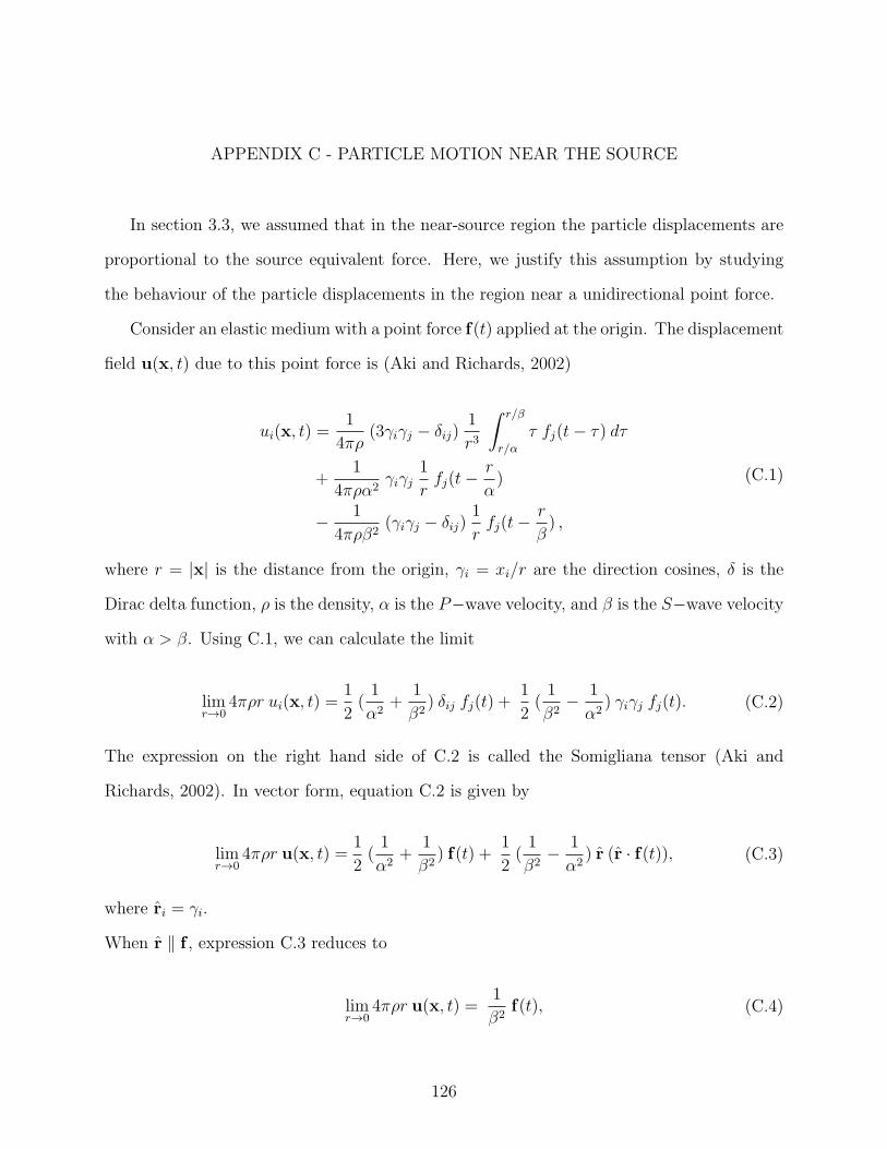
APPENDIX C - PARTICLE MOTION NEAR THE SOURCE
In section 3.3, we assumed that in the near-source region the particle displacements are
proportional to the source equivalent force. Here, we justify this assumption by studying
the behaviour of the particle displacements in the region near a unidirectional point force.
Consider an elastic medium with a point force f(t) applied at the origin. The displacement
field u(x, t) due to this point force is (Aki and Richards, 2002)
ui(x, t) =1
4πρ(3γiγj − δij)
1
r3
∫ r/β
r/α
τ fj(t− τ) dτ
+1
4πρα2γiγj
1
rfj(t−
r
α)
− 1
4πρβ2(γiγj − δij)
1
rfj(t−
r
β) ,
(C.1)
where r = |x| is the distance from the origin, γi = xi/r are the direction cosines, δ is the
Dirac delta function, ρ is the density, α is the P−wave velocity, and β is the S−wave velocity
with α > β. Using C.1, we can calculate the limit
limr→0
4πρr ui(x, t) =1
2(
1
α2+
1
β2) δij fj(t) +
1
2(
1
β2− 1
α2) γiγj fj(t). (C.2)
The expression on the right hand side of C.2 is called the Somigliana tensor (Aki and
Richards, 2002). In vector form, equation C.2 is given by
limr→0
4πρr u(x, t) =1
2(
1
α2+
1
β2) f(t) +
1
2(
1
β2− 1
α2) r (r · f(t)), (C.3)
where ri = γi.
When r ‖ f , expression C.3 reduces to
limr→0
4πρr u(x, t) =1
β2f(t), (C.4)
126

and when r ⊥ f(t), expression C.3 reduces to
limr→0
4πρr u(x, t) =1
2(
1
α2+
1
β2) f(t). (C.5)
In both situations the displacement at the source location is parallel to the excitation. This
result is confirmed by Wu and Ben-Menahem (1985) who show (in Figure 2 of their paper)
the motion of the elastodynamic field in the near-source region of a unidirectional force.
127
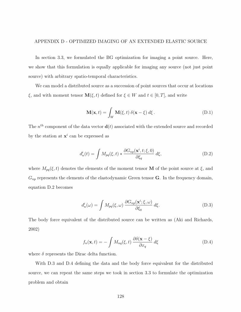
APPENDIX D - OPTIMIZED IMAGING OF AN EXTENDED ELASTIC SOURCE
In section 3.3, we formulated the BG optimization for imaging a point source. Here,
we show that this formulation is equally applicable for imaging any source (not just point
source) with arbitrary spatio-temporal characteristics.
We can model a distributed source as a succession of point sources that occur at locations
ξ, and with moment tensor M(ξ, t) defined for ξ ∈ W and t ∈ [0, T ], and write
M(x, t) =
∫W
M(ξ, t) δ(x− ξ) dξ . (D.1)
The nth component of the data vector d(t) associated with the extended source and recorded
by the station at xi can be expressed as
din(t) =
∫Mpq(ξ, t) ∗
∂Gnp(xi, t; ξ, 0)
∂ξqdξ, (D.2)
where Mpq(ξ, t) denotes the elements of the moment tensor M of the point source at ξ, and
Gnp represents the elements of the elastodynamic Green tensor G. In the frequency domain,
equation D.2 becomes
din(ω) =
∫Mpq(ξ, ω)
∂Gnp(xi; ξ, ω)
∂ξqdξ. (D.3)
The body force equivalent of the distributed source can be written as (Aki and Richards,
2002)
fn(x, t) = −∫Mnq(ξ, t)
∂δ(x− ξ)∂xq
dξ (D.4)
where δ represents the Dirac delta function.
With D.3 and D.4 defining the data and the body force equivalent for the distributed
source, we can repeat the same steps we took in section 3.3 to formulate the optimization
problem and obtain
128

ajp(ω)
∫W
Gi∗rnG
jrp dx =
∫eiωTM∗
pq(ξ, ω)∂G∗np(x
i; ξ, ω)
∂ξqdξ, (D.5)
which can be simplified using D.3 as
ajp(ω)
∫W
Gi∗rn G
jrp dx = eiωT di∗n . (D.6)
Equation D.6 represents a system of equations that can be concisely expressed as
Γ(ω) a(ω) = eiωT d∗(ω), (D.7)
which has the exact form as equation 3.12 we obtained for a point source in section 3.3.
129

APPENDIX E - BLENDED NEIGHBOR INTERPOLATION
Blended neighbor interpolation (Hale, 2009) is designed specifically to facilitate tensor-
guided interpolation of scattered data.
If we assume the scattered data to be interpolated are a set
F = {f1, f2, ..., fK} (E.1)
of K known sample values fk ∈ R corresponding to a set
X = {x1,x2, ...,xK} (E.2)
of K known sample points (coordinates) xk ∈ Rn, then the goal of interpolation is to use
the known samples to construct a function q(x) : Rn → R such that q(xk) = fk.
In the blended neighbor interpolation method (Hale, 2009), the interpolant q(x) is con-
structed in two steps:
(i) Solve the eikonal equation
∇t(x) · D(x) · ∇t(x) = 1 , x /∈ χ ;
t(xk) = 0 , xk ∈ χ (E.3)
for t(x): non-Euclidean distance from x to the nearest known sample xk, and
p(x): the value fk of the sample at point xk nearest to the point x.
(ii) Solve the blending equation
q(x)− 1
2∇ · t2(x)D(x) · ∇q(x) = p(x) (E.4)
for the blended neighbor interpolant q(x).
In the equations above, D is a metric tensor field which defines the measure of distance in
space by providing the anisotropic and spatially varying coefficients of the eikonal equation.
130

In n dimensions, the metric tensor field D is a symmetric and positive definite n× n matrix
(Hale, 2009).
131

APPENDIX F - COMBINING MEASUREMENTS HAVING RANDOM
UNCORRELATED ERRORS AND KNOWN VARIANCES
Here, we discuss a way to combine independent measurements of a quantity using a
weighted averaging scheme.
Consider N independent measurements (x1, x2, ..., xN) of the same quantity where each
measurement has an unknown expected value and error, i.e.,
xi = µ+ ei, i = 1, 2, ..., N (F.1)
where µ is the true value of the quantity we wish to estimate, and ei is the error in each
measurement.
We assume that the errors are not correlated, their expected values are zero, and their
variances σ2i are known.
We let the combined measurement x to be a weighted average (linear combination) of
the individual measurements xi,
x =N∑i=1
wixi, (F.2)
requiring that the weights wi must satisfy the unbiasedness condition
N∑i=1
wi = 1. (F.3)
Using these assumptions, the variance of the combined measurement can be expressed as
σ2 =N∑i=1
w2i σ
2i . (F.4)
132

By minimizing this variance with respect to wi (subject to the unbiasedness constraint
of F.3) the weights wi can be determined as
wi =
1σ2i
N∑j=1
1
σ2j
, i = 1, 2, ..., N. (F.5)
Using these weights, we can compute the best (minimum variance) estimate for the combined
measurement x and its variance σ2 using equations F.2 and F.4, respectively. Note that to
arrive at these results, we assumed no particular statistical distribution for the measurement
errors.
133