optimisation of trajectories for wireless power
TRANSCRIPT

https://doi.org/10.1007/s10846-018-0824-6
Optimisation of Trajectories for Wireless Power Transmissionto a Quadrotor Aerial Robot
Murray L. Ireland1 ·David Anderson1
Received: 15 November 2016 / Accepted: 26 March 2018© The Author(s) 2018
AbstractUnmanned aircraft such as multirotors are typically limited in endurance by the need to minimise weight, often sacrificingpower plant mass and therefore output. Wireless power transmission is a method of delivering power to such aircraft froman off-vehicle transmitter, reducing weight whilst ensuring long-term endurance. However, transmission of high-poweredlasers in operational scenarios carries significant risk. Station-keeping of the laser spot on the receiving surface is crucial toboth ensuring the safety of the procedure and maximising efficiency. This paper explores the use of trajectory optimisation tomaximise the station-keeping accuracy. A multi-agent model is presented, employing a quadrotor unmanned rotorcraft andenergy transmission system, consisting of a two-axis gimbal, camera sensor and laser emitter. Trajectory is parametrised interms of position and velocity at the extremes of the flight path. The optimisation operates on a cost function which considerstarget range, beam angle of incidence and laser spot location on the receiving surface. Several cases are presented for arange of variables in the trajectory and different conditions in the model and optimisation algorithm. Results demonstratethe viability of this approach in minimising station-keeping errors.
Keywords Trajectory optimisation · Quadrotor · Wireless power transmission · Simulated annealing · Nelder-Mead
1 Introduction
Wireless power transmission (WPT) is the transfer of elec-trical power without relying on standard contact media suchconductors or wires. Although the concept is not a newone [8], advancement of power transmitters and photosen-sitive receivers has made it more appealing in recent years.Whilst early investigations considered the use of microwaveenergy [7], several recent research programmes have favouredlasers [11, 18] especially for long-range transmission. WPTis particularly beneficial to systems which are limited inenergy capacity, or which draw a large amount of powerwith respect to their total energy reserves.
� Murray L. [email protected]
David [email protected]
1 School of Engineering, James Watt (South) Building,University of Glasgow, Glasgow G12 8QQ, UK
An important contemporary example of such a systemis the unmanned aerial vehicle (UAV). To remain airborne,an aircraft must generate enough lift to overcome its ownweight. Weight minimisation is therefore a key considera-tion in the design of any aircraft and is especially so forrotorcraft, where the lifting force is produced exclusively byits rotors. Consider a rotorcraft with an all-electrical powersystem as typically favoured by UAVs, which draws powerfrom an on-board cell array or battery. As the rotors areresponsible for both balancing the weight and providingmanoeuvring control of the vehicle, rotor power consump-tion is typically much higher than for fixed-wing aircraft ofequivalent mass. Whilst it is possible to increase the energyavailable to the rotor or rotors by increasing the battery sizeor adding further cells, this only adds further weight andthus requires a greater lifting force. Further increasing thepower consumption may then negate any potential bene-fits to flight time. This is particularly problematic in microUAVs, or micro air vehicles (MAV), where the power supplycontributes to a large fraction of the total vehicle mass.
Rather than attempt to compromise between the UAV’sweight and endurance, consider an alternative. The UAVcould carry only a minimal power supply, thus reducing its
Journal of Intelligent & Robotic Systems (2019) 95: –
/ Published online: 9 April 2018
675 584

weight. The flight time could then be extended indefinitelyby supplying power remotely, using WPT. The operationalbenefits of such a hyper-extended endurance aircraft arenumerous. Practical WPT could be implemented using eitherof two approaches. The first involves continuous WPT powersupply, reducing the requirements of on-board power supplyto emergency scenarios only. The second approach involvesintermittent WPT supply, recharging a larger, but still limited,on-board battery at frequent intervals.
The feasibility of this approach has been demonstratedwith application to both rotary- [1, 19] and fixed-wing [20]aircraft, all employing laser-based WPT. Some limitationsin the demonstrated systems are evident. In the 12-hourquadrotor flight conducted by [1], the quadrotor’s move-ment was restricted in the horizontal plane to a square ofside 5 m. This was primarily to ensure that the laser remainedon-target, thus minimising the risk of the laser strikinganother surface. Whilst such safeguards are necessary inearly testing, restricting the movement of the quadrotornaturally limits its usefulness in many applications.
The primary concern with allowing unrestricted move-ment of the receiving system during WPT is the possibilityof the laser missing its target and striking another surface,or missing the aircraft entirely. Given the power involvedin such transmissions, this could be catastrophic. Addition-ally, poor station-keeping of the incident laser spot reducesthe energy received by the system. These concepts are illus-trated in Fig. 1. The laser can strike a surface other than theintended under two conditions. The first is that the beamdiameter is greater than the projected dimensions of thereceiving surface. Assuming the surface has been designedto be sufficiently large, this overfill has two potential causes:divergence of the beam over great distances; or a sufficientlylarge angle between the incident laser vector and the surfacenormal. The second condition is that the laser beam partiallyor entirely misses its target due to poor beam-steering. This
Fig. 1 Visualisation of laser beam on-target (left), overfilling dueto poor angle of incidence (centre) and partially missing due topoor beam-steering (right). (Note: laser beamwidth is enlarged forillustrative purposes)
may be caused by the receiving system manoeuvring tooaggressively for the laser beam-steering system to keep up.
In allowing a UAV such as the quadrotor to freely per-form its mission without heavy restrictions on movement,these hazards must be considered. One way to minimisethe likelihood of tracking errors is to combine the quadro-tor flight controller and laser beam-steering system trackingcontrollers into a single control system. However this archi-tecture introduces additional complexity and robustnessissues such as timely agent communication, lack of auton-omy and swarm architecture inflexibility. Before proceedingapace with the design of such a complex, integrated controlsystem it is worthwhile pausing to quantify the performancebenefits obtainable from altering each controller’s designaims, in particular optimising the UAV’s flight trajectorysuch that the risk of beam overfilling or target miss areminimised or, ideally, eliminated.
This paper presents preliminary results of applying suchan optimisation to the quadrotor guidance loop. The optimisa-tion problem is presented as the minimisation of geometricerrors in a multi-agent dynamic system. First, models of theagents in this system are discussed, including any relevantsubsystems. Next, the optimisation problem is specified,including the errors to be minimised and the manipulatedvariables which enable this. A selection of results showingoptimised trajectories are then presented and discussed. Finally,conclusions and future research directions are presented.
2Modelling theMulti-agent Problem
The optimisation problem presented in this paper isspecified as the minimisation of specific errors relating tothe relative pose of two distinct agents. The first agentis the quadrotor aerial robot, which receives power via aphotovoltaic array mounted on its frame. The second agentis an actuated energy transmission system (ETS), whichconsists of a laser emitter and electro-optical (EO) cameramounted on a two-axis gimbal, allowing accurate targettracking and sightline control. The gimbal is in the standardelevation-over-azimuth configuration affording the ETS’slaser emitter and camera rotational freedom in elevation andheading [3, 4].
During ideal operation, the laser emitter projects a beamalong a vector which is required to intersect with thegeometric centre of the quadrotor’s photovoltaic array. TheEO camera is mechanically aligned to the laser emitter andprovides feedback to the ETS’s control system via “see-spot” tracking of the laser spot on the photovoltaic detector.It is thus necessary to consider the position and orientationof the photovoltaic sensor relative to both the laser emitterand EO camera. This requires accurate simulation of thegeometry and dynamics of both systems.
568 J Intell Robot Syst (2019) 95: –567 584

2.1 Multi-agent Geometry
The geometry of the multi-agent system can be seen inFig. 2. Both agents operate in an inertially-fixed Worldframe W . For brevity, the reference frame W is impliedin the cases where a position vector r or element lacksa superscript denoting an explicit frame of reference. Themechanics of the quadrotor are covered extensively in theliterature and will not be described in depth here. For moredetail, the reader is referred to [6, 12, 13, 21].
First consider the quadrotor. The quadrotor has sixdegrees of freedom: translational displacement rQ =[xQ, yQ, zQ]T ∈ R
3 and rotational displacement η =[φ, θ, ψ]T ∈ R
3. A body-fixed frame Q has origin at thequadrotor’s centre of mass. The orientation of Q in W isgiven by the direction cosine matrix
RWQ =
⎡⎣
cφcψ sφsθ cψ − cφsψ cφsθ cψ + sφsψcφsψ sφsθ sψ + cφcψ cφsθ sψ − sφcψ
−sθ sφcθ cφcθ
⎤⎦ (1)
where cφ denotes cos φ, sθ denotes sin θ and so forth. Thisallows any position in Q to be rotated to W by rW =RWQ rQ. As R ∈ SO(3), the reverse transformation may be
defined RQW = (RW
Q )T .The geometric centre of the quadrotor’s photovoltaic sen-
sor has fixed position rQS/Q ∈ R3 in Q, as shown Fig. 2. The
Fig. 2 Geometry of quadrotor and ETS agents, with associatedsubsystems, in inertial frame W
orientation of the sensor surface is defined by the surfacenormal nQS ∈ R
3. The sensor thus has position and surfacenormal in W defined by
rS = rQ + RWQ rQS/Q
nS = RWQ nQS
The geometry of the ETS and its subsystems may beconsidered similarly. Consider Fig. 3. The ETS has twodegrees of freedom: elevation ε and azimith λ. These statesdescribe the rotational displacement of an actuated platformwhich is driven by two brushless motors (see [2] for detailsof the full equations of motion). The intersection of theelevation and azimuth axes has fixed position rE in W . Thisposition is taken as the origin of a reference frame E , whichis fixed on the actuated platform. The orientation of E in Wis then given by the direction cosine matrix
RWE =
⎡⎣
cos ε cos λ − sin λ sin ε cos λ
cos ε sin λ cos λ sin ε sin λ
− sin ε 0 cos ε
⎤⎦ (2)
with the reverse transformation REW = (RW
E )T applying.The ETS’s EO camera and laser emitter are fixed on
the actuated platform. The EO camera has fixed positionrEC/E ∈ R
3 and line of sight unit direction vector nC ∈ R3 in
Fig. 3 Axes definition of reference frame E , fixed on the ETS’sactuated platform
J Intell Robot Syst (2019) 95: –567 584 569

E . The camera position and line of sight are thus describedin W by
rC = rE + RWE rEC/E
nC = RWE nEC
The laser similarly has source position rEL/E ∈ R3 and
unit direction vector nL ∈ R3 in E . The position and
direction vector in W are thus
rL = rE + RWE rEL/E
nL = RWE nEL
The geometry described here and shown in Fig. 2 maybe used to define the errors for the optimisation problem.The agent geometry and thus the optimisation errors aresubject to the dynamics and subsystem behaviours of thetwo agents, which may now be defined.
2.2 The Quadrotor
The quadrotor’s propulsion and control are provided by fourrotors, each with input ui , i = {1, 2, 3, 4}. The translationaland rotational response of the quadrotor to inputs in ui
is described by a non-linear rigid body model. A non-linear dynamic inversion (NDI) controller with a linear statefeedback provides a critically-damped response in closedloop [13].
2.2.1 Vehicle Dynamics
The response of the quadrotor position rQ and attitude η inW to inputs in u = [u1, u2, u3, u4]T is described by
rQ = gz − KT
mRWQ zucol
η = I−1
⎛⎝
⎡⎣
KT Lulat
KT Lulong
KQuyaw
⎤⎦ − η × Iη
⎞⎠ (3)
where m is the quadrotor mass, g is the acceleration dueto gravity, KT and KQ are thrust and torque constants,respectively and z is the unit direction vector in the z-axis.The inertia tensor I is the diagonal matrix
I =⎡⎣
Ix 0 00 Iy 00 0 Iz
⎤⎦
Equation 3 describes the elements of the pseudo-inputvector
u∗ = [ucol, ulat, ulong, uyaw]T
rather than the true inputs. This simplifies the definitionof the model and control of the plant. The pseudo-inputs
are then related to the true inputs by the invertible matrixrelationship
u∗ =
⎡⎢⎢⎣
1 1 1 10 0 1 −1
−1 1 0 0−1 −1 1 1
⎤⎥⎥⎦u (4)
2.2.2 Controller
An NDI controller is used to render the closed-loopdynamics of the quadrotor near-linear and simplify thegain-selection process. This ensures accurate trackingof specified trajectories. The four pseudo-inputs definedpreviously are specified by the control laws
ucol = m[g − Kz1(zd − z) − Kz2(zd − z)
]
KT cos φ cos θ
ulat = 1
KT L
[Ix
(Ka1(φd − φ) − Ka2φ
)
+(Iz − Iy)θ ψ]
ulong = 1
KT L
[Iy
(Ka1(θd − θ) − Ka2θ
)
+(Ix − Iz)φψ]
uyaw = 1
KQ
[Iy
(Kψ1(ψd − ψ) − Kψ2ψ
)
+(Iy − Ix)φθ]
(5)
where zd and ηd are specified by the state feedback
[zd
ηd
]=
⎡⎢⎢⎣
Kz1 0 0 00 Ka1 0 00 0 Ka1 00 0 0 Kψ1
⎤⎥⎥⎦
[zd − z
ηd − η
]
+
⎡⎢⎢⎣
Kz2 0 0 00 Ka2 0 00 0 Ka2 00 0 0 Kψ2
⎤⎥⎥⎦
[zd − z
−η
](6)
which controls the three rotational degrees of freedom inη and the height z. For clarity, the subscript Q has beenomitted from the position elements in these equations. Thetrue inputs u are then obtained by inverting the relationshipin Eq. 4.
To stabilise the zero dynamics, φd and θd must be definedsuch that a desired position in the horizontal plane xW -yW
is reached. This is achieved by the non-linear feedbacks
φd = − arcsin
[m(xd sin ψ − yd cos ψ)
KT ucol
]
θd = − arcsin
[m(xd cos ψ + yd sin ψ)
KT ucol cos φ
](7)
J Intell Robot Syst (2019) 95: –567 584570

where xd and yd are specified by the state feedback[
xd
yd
]= Kp1
[xd − x
yd − y
]+ Kp2
[xd − x
yd − y
](8)
The trajectory commands rQ,d = [xd, yd, zd ]T and theirderivatives are each specified by a polynomial function oftime. The parameters of these polynomials are then thevariables which are adjusted by the optimisation algorithm.This is described in more detail in the problem specification.
The heading command ψd is specified by a line-of-sight controller which points the horizontal component ofthe photovoltaic sensor’s surface normal in the directionof the ETS. Assuming this surface normal is aligned suchthat yQ · nQS = 0, the quadrotor’s yaw command may bespecified by
ψd = arctanyE − yQ
xE − xQ(9)
2.3 An Energy Transmission System
The ETS is modelled as a simple two degree-of-freedomsystem with first-order rotational dynamics. The inputsto the brushless motors may be considered the set-pointcommands for each degree of freedom, that is uE =[εd, λd ]T . These commands are specified by a beam-steering controller which has multiple modes. Two of thesemodes rely on visual feedback from the EO camera.
2.3.1 Platform Dynamics
The response in elevation and azimuth angles to the set-pointcommands is described by the first-order relationships[
ε
λ
]= 1
τ
(uE −
[ε
λ
])(10)
where τ represents an abstraction of the electro-mechanicalbehaviour of the motors and the inertias of the ETSstructure.
2.3.2 EO Camera Model
The EO camera tracks the photosensitive sensor and thelaser spot when it is incident on the sensor. The coordinatesof the sensor and laser spot in the camera image are thenprovided to the ETS controller. A suitable camera model isthus required (Fig. 4).
The position of a point P, fixed in the quadrotor bodyframe Q may be described in the ETS platform-fixed frameE by transforming it first to W and then E . The position ofP rP is thus described relative to the camera position rC inE by
rEP/C = REW
(rQ − rE + RW
Q rQP/Q
)− rEC/E (11)
Camera
centre Principal axis
Image plane
Fig. 4 Geometry of a generic pinhole camera model. The cameracentre C is at the centre of the coordinate system, with position rC inEuclidean 3-space. A point P has position rP/C relative to C in 3-space.This point may be mapped to 2-space by considering the intersectionof the relative position vector with the image plane. The image planeis normal to the principal axis x and is fixed at point p along this axis
If rEP/C = [xEP/C, yEP/C, zEP/C]T describes the position of Pin object space, the position in camera space is described by
xCP = fyEP/C
xEP/C
yCP = −fzEP/C
xEP/C
(12)
The camera has field of view ϕ and aspect ratio A. ForP to be visible to the camera, it must therefore satisfy theconstraints
−f tan ϕ ≤ xCP ≤ f tan ϕ
−f
Atan ϕ ≤ yCP ≤ f
Atan ϕ
2.3.3 Laser Model
The laser beam is modelled as a beam of finite length,originating at the point rL, which is fixed in E . Thebeam terminates at the laser spot position rLS, where itintersects the surface plane of the photovoltaic sensor on thequadrotor. The laser spot position may be given by
rLS = lnL + rL (13)
where l is the beam length from source to terminal.The laser spot only exists if it intersects this plane within
the area defined by the sensor surface. Otherwise, the beamlength is assumed to be infinite. Assuming a circular sensorsurface of radius rS and centre rS, the beam length is thusdefined by
l ={
(rS−rL)·nSnL·nS
if ‖p − rS‖ ≤ rS
∞ if ‖p − rS‖ > rS(14)
J Intell Robot Syst (2019) 95: –567 584 571

where p is the point of intersection of the laser vector andthe infinite surface plane of the sensor.
2.3.4 Beam-Steering Controller
The purpose of the ETS controller is to ensure that the laserspot remains incident on the photovoltaic sensor and close toits centre at all times. Whilst no “off” state for the laser beamis included in the model, it is assumed that the laser is notactivated until there is confidence that it will be immediatelyincident on the surface. To achieve this, it has three modes.
First, seek mode directs the principal axis of the EOcamera towards the quadrotor position rQ, which is knownand communicated to the ETS. This is achieved using thesimple sightline controller
tan λd = − zQ − zE√(xQ − xE)2 + (yQ − yE)2
tan εd = yQ − yE
xQ − xE(15)
The quadrotor is assumed to be at sufficient distance andthe camera assumed to have sufficient field of view that thisoperation will result in the camera visually acquiring thequadrotor.
The controller then enters sensor tracking mode. Thesensor is modelled as having a ring of LEDs around itscircumference, which are now visible to the EO camera.The centroid of the N LEDs then corresponds to the sensorposition rS and is found in camera space C from
rCS = 1
N
N∑i=1
rCi
where ri describes the position of some LED i.A proportional-integral (PI) controller then drives the
system to centre rCS within the camera frame, with thecontrol law
uE = τ
(Kpe + Ki
∫e dt
)+
[ε
λ
](16)
where the error e ∈ R2 is simply the coordinates of the
centroid in camera space e = rCS .When the LED centroid is centred in C within some
tolerance, the controller enters laser spot tracking mode.The controller acts to centre the laser spot, now incident onthe sensor surface, at the sensor position rS. The controllerdescribed by Eq. 16 is again used, whilst the error is nowspecified by
e = rCS − rCLS (17)
3 The Optimisation Problem
The optimisation problem is presented as the minimisationof three geometric errors by way of 18 possible variables.These variables describe the commanded trajectory of thequadrotor. The errors describe the relative geometries ofthe two agents, and are thus subject to the dynamics andsubsystems of these agents.
3.1 Optimisation Variables: Describing theTrajectory
The desired trajectory rQ,d = [xd, yd, zd ]T of the quadrotoris specified in each degree of freedom by a fifth-orderpolynomial [5, 10]. The desired trajectory in x is thusexpressed by
xd(t) = a0 + a1t + 1
2a2t
2 + 1
6a3t
3
+ 1
12a4t
4 + 1
20a5t
5 (18)
Differentiating this expression provides the desired trajec-tory of x
xd (t) = a1 + a2t + 1
2a3t
2 + 1
3a4t
3 + 1
4a5t
4 (19)
whilst the desired trajectory of x may be found similarly
xd (t) = a2 + a3t + a4t2 + a5t
3 (20)
The time at the beginning of the trajectory may bedenoted t0 and the time at the end tf . Then if xd(t0) =x0, xd (tf ) = xf and so forth, it is possible to relate thedesired position, velocity and acceleration at each end ofthe trajectory to the coefficients ai, i = {1, 2, 3, 4, 5} by thematrix relationship
⎡⎢⎢⎢⎢⎢⎢⎣
x0
x0
x0
xf
xf
xf
⎤⎥⎥⎥⎥⎥⎥⎦
=
⎡⎢⎢⎢⎢⎢⎢⎢⎣
1 t012 t2
016 t3
01
12 t40
120 t5
00 1 t0
12 t2
013 t3
014 t4
00 0 1 t0 t2
0 t30
1 tf12 t2
f16 t3
f1
12 t4f
120 t5
f
0 1 tf12 t2
f13 t3
f14 t4
f
0 0 1 tf t2f t3
f
⎤⎥⎥⎥⎥⎥⎥⎥⎦
⎡⎢⎢⎢⎢⎢⎢⎣
a0
a1
a2
a3
a4
a5
⎤⎥⎥⎥⎥⎥⎥⎦
(21)
For any desired x0, xf and their derivatives, the coeffi-cients of the smooth polynomials xd(t) and xd (t) may befound by solving Eq. 21 for a0, a1, . . . a5. The desired tra-jectories in y and z are constructed similarly. Thus, thedesired trajectory in each degree of freedom may be deter-mined by specifying initial and final conditions for time,position, velocity and acceleration. The trajectory commandsfor position and velocity at any time t are then supplied tothe quadrotor controller, as described by Eqs. 5 to 8.
J Intell Robot Syst (2019) 95: –567 584572

In this instance, it is assumed that t0 = 0, whilst tf isfixed for a given manoeuvre. This leaves the 18 possiblevariables, {r0, r0, r0, rf , rf , rf } ∈ R
3. The complete set ofpossible variables is defined as
χ = [rT0 , rT
0 , rT0 , rT
f , rTf , rT
f ]T ∈ R18 (22)
Rather than optimise the trajectory for all variables χ , asubset χ ⊆ χ is defined. The remaining variables in χ arefixed constant. This allows the viability of this trajectorygeneration method to be considered on a smaller scale.
3.2 Errors
The cost function employed in the optimisation describesthree scalar errors, each related to the geometry of thequadrotor-ETS system. Each error ei, i = {1, 2, 3} isweighted by a scalar Qi or matrix Qi and normalised withrespect to a nominal maximum Mi .
Recall the description of the laser interaction with thephotovoltaic sensor, illustrated in Fig. 1. To minimise thepossibility of overfilling or partially missing the sensor, theprojected area of the sensor in the direction of the laservector must be maximised. This is achieved by consideringthe angle of incidence γ between the sensor normal and thelaser vector, given by
cos γ = −nS · nL (23)
The yaw autopilot described by Eq. 9 acts to minimiseγ in the horizontal plane. The quadrotor trajectory is thenoptimised to aid the yaw autopilot and produce an attitudewhich minimises the angle in in the vertical plane. Thus, tominimise the expression (cos γd −cos γ ), where γd = 0, theerror function e1 is defined
e1 = Q1
M21
(1 + nT
S nL
)2(24)
where M1 = 1 and Q1 = 1.The trajectory pursued by the quadrotor also impacts
the beam-steering accuracy of the ETS. To avoid defininga trajectory which is too aggressive for accurate beam-steering, the error between the centroid of the photovoltaicsensor rS and the laser spot position on the sensor rLS isminimised by
e2 = 1
M22
(rLS − rS)T Q2 (rLS − rS) (25)
where M2 = 0.05 and
Q2 =⎡⎣
1 0 00 1 00 0 1
⎤⎦
Finally, the the distance between the laser emitter andthe receiving sensor is minimised. This minimises beamdivergence and reduces the energy loss due to atmosphericattenuation. The error is simply
e3 = 1
M23
(rS − rL)T Q3 (rS − rL) (26)
where M3 = 50 and
Q3 =⎡⎣
0.001 0 00 0.001 00 0 0.001
⎤⎦
3.3 Cost Function
The optimisation problem is then formulated as a costfunction (χ) which is subject to the dynamics, controllersand trajectories of both agents. The problem is thusspecified by
minχ⊆χ∈R18
(χ) for t ∈ [t0, tf ]subject to xQ(t) = fQ
(xQ(t), rQ,d (t), ψd(t)
)
xE(t) = fE (xE(t), uE(t))
rQ,d (t) = gQr (χ , t0, tf )
ψQ,d (t) = gQψ(xQ(t), xE(t))
uE(t) = gE(xQ(t), xE(t)) (27)
where fQ describes the closed-loop quadrotor dynamics andcontroller, fE describes the closed-loop ETS response, gQr
and gQψ respectively describe the trajectory and headingcommands of the quadrotor and gE describes the ETS panand tilt commands.
The cost function (χ) is then specified as
(χ) =∫ tf
t0
[e1(t) + e2(t) + e3(t)] dt (28)
where the errors {e1, e2, e3} ≥ 0 ∈ R are dependent on therelevant geometry of the multi-agent system.
3.4 Algorithm
The trajectory is optimised by the non-linear Nelder-Mead method first proposed by [17] and adapted by [15].This approach employs a simple line-search algorithmto accurately identify local minima. In one of thecases presented, simulated annealing is employed toapproximately determine the global minima within aspecific search space. This method was independentlydeveloped by [14] and [9]. Both algorithms were inspired bya mathematical model of the physical process of annealing,which was developed by [16].
J Intell Robot Syst (2019) 95: –567 584 573

4 Results
The optimisation is performed in MATLAB and considersa specific scenario. A quadrotor with a photovoltaic sensorenters a volume of space, at which time the ETS visuallyacquires the sensor and emits the laser onto its surface. Thequadrotor then follows a curved flight path which is definedby the variables described in Eq. 22. The quadrotor followsthis flight path for a short period of time before leaving theETS’s volume of interest. This scenario is designed to pro-vide a specific test case and does not necessarily reflect thereality of a WPT operation. Methods of increasing the realismof the simulation are discussed at the end of the paper.
Whilst there are 18 possible variables which can be selectedby the optimisation, there is no particular requirement tovary all 18. Instead, subsets of χ are optimised, whilstthe remaining “variables” are held constant. Three suchsubsets are considered. The first subset describes only twovariables, the second considers four and the third considerssix. For each subset, two different cases are considered.
4.1 Simulation Setup
The quadrotor is commanded to follow a trajectory rQ,d (t),beginning at t0 = 0 and finishing at tf . The ETS ispositioned at the origin of the x-y plane in W . The quadrotorstarts with some position r0 = [0, y0, z0]T and has finaldestination rf = [0, yf , zf ]T . The accelerations commandsr0 and rf are fixed at zero in each case. The initial andfinal velocities, r0 and rf respectively, then define the flighttrajectory.
The simulation is initialised such that the laser vector nL
is in the direction of the sensor position rS. This is done toreduce large values in the optimisation errors which wouldswamp smaller errors and reduce the effectiveness of theoptimisation. The quadrotor is similarly yawed such that thesensor normal nS is in the direction of the ETS position rE.
The simulation models use properties taken from systemidentification of the Qball-X4 quadrotor, supplied byQuanser,1 and a bespoke ETS system. These properties areprovided in Table 1, at the end of the paper.
4.2 Optimisation with Two Variables
The trajectory is parameterised by two variables χ ={x0, xf }, whilst the remainder of the parameter set χ\χ isconstant. The optimisation is performed for two cases. Thefirst is a 10 s flight at short range, whilst the second is a20 s flight at longer range. For each case, the quadrotor tra-
1Quanser Consulting, Inc http://www.quanser.com
jectory is optimised for WPT using the two aforementionedvariables only.
4.2.1 Case 1: 10 s
The quadrotor trajectory is defined by the initial positionr0 = [0, 10,−2]T at t0 = 0 s and final positionrf = [0, −10, −2]T at tf = 10 s. The constant velocityparameters are fixed at {y0, z0, yf , zf } = 0. The trajectoryis optimised for the two-parameter set χ = {x0, xf } overthe time range [t0, tf ], with initial values χ0 = {5, −5}.
Employing the Nelder-Mead line-search algorithm, alocal minima is identified at the coordinates given inTable 3. The resulting trajectory is shown in Fig. 5.Asymmetry in the trajectory about the x-axis is immediatelyevident. The constituent errors and cumulative cost functionduring a flight with the optimised trajectory parameters canbe seen in Fig. 6. Here, it can be seen that the error relatingto beam angle of incidence, e1, is largest at the end of thetrajectory. Conversely, the error relating to the laser spotposition on the sensor, e2, dominates at the beginning of thetrajectory. This is caused by initial beam-steering errors inthe ETS’s visual tracking system as the quadrotor enters itsfield of perception. Thus, the large difference in velocityfor the initial and final trajectory properties is clearly dueto the optimisation algorithm pursuing two goals. First,to reduce e1 at the end of the trajectory, it increases thedesired velocity at this location xf . This adjusts the shapeof the trajectory such that the vehicle attitude during thefinal second minimises e1. The second goal, reducing thelarge spot position error e2, requires that the initial velocitycommand x0 is reduced. This improves the ETS’s ability tovisually capture the photovoltaic sensor and centre the laserspot upon it. The resulting minimised cost function at theend of the flight is min = 0.455.
For the two-variable optimisation, Eq. 27 may beconsidered a non-linear function of two properties, x0 andxf , with a single output . This may be representedgraphically as a two-dimensional contour map withelevation , as shown in Fig. 7. The contour map confirmsthat a local minima has been identified by the optimisationalgorithm. Owing to the complexity of the non-linearfunction in this instance, it cannot be stated with anycertainty that a global minima has been found.
4.2.2 Case 2: 20 s
The quadrotor trajectory is defined by the initial positionr0 = [0, 20,−3]T at t0 = 0 s and final position rf = [0, −20,−3]T at tf = 20 s. The constant velocity parametersare fixed at {y0, z0, yf , zf } = 0. The trajectory is optimised
J Intell Robot Syst (2019) 95: –567 584574

Table 1 Simulation modelproperties Property Symbol Value Unit
EO camera aspect ratio A 0.75 –
EO camera focal length f 601.8 pixel
Moment of inertia about xQ Ix 0.032 kg m2
Moment of inertia about yQ Iy 0.033 kg m2
Moment of inertia about zQ Iz 0.041 kg m2
Quadrotor attitude controller gain Ka1 380.25 –
Quadrotor attitude controller gain Ka2 39 –
ETS controller integral gain Ki 2.5274 –
ETS controller proportional gain Kp 0.1296 –
Quadrotor position controller gain Kp1 3.8025 –
Quadrotor position controller gain Kp2 3.9 –
Quadrotor height controller gain Kz1 3.8025 –
Quadrotor height controller gain Kz2 3.9 –
Quadrotor yaw controller gain Kψ1 0.6084 –
Quadrotor yaw controller gain Kψ2 1.56 –
Torque gain KQ 1.919 N m
Thrust gain KT 119.6 N
Moment arm of rotors L 0.2 m
Quadrotor mass m 1.512 kg
Number of sensor diodes N 8 –
Direction vector of camera in E nEC [1, 0, 0]T –
Direction vector of laser beam in E nEL [1, 0, 0]T –
Surface normal of sensor in Q nQS [0.995, 0, 0.0998]T –
Radius of sensor rS 0.05 m
Position of camera in E rEC/E [0, 0.01, 0]T m
Position of laser emitter in E rEL/E [0, −0.01, 0]T m
Position of sensor in Q rQS/Q [0, 0, 0.1]T m
ETS response time constant τ 0.1 s
Camera horizontal field of view ϕ 56 ◦
x (m)
05101520
y (m
)
-10
-5
0
5
10
Fig. 5 Near-optimal trajectory for a 10 s flight, determined by atwo-parameter optimisation. Height remains constant at z(t) = −2 m
for the two-parameter set χ = {x0, xf } over the time range[t0, tf ], with initial values χ0 = {5, −5}.
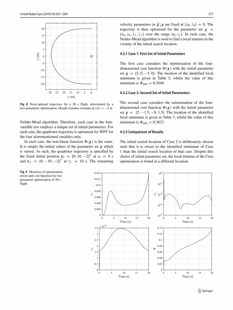
Again employing the Nelder-Mead algorithm, a localminima is identified at the coordinates given in Table 3.The resulting trajectory is shown in Fig. 8. The trajectoryhas noticeably greater symmetry about the x-axis in thisinstance. This property is complemented by the similarinitial and final velocity parameters after optimisation. Theconstituent error histories and cumulative cost functionduring this longer flight are provided in Fig. 9. It is clearthat the most heavily-weighted errors—those relating tothe beam angle of incidence, e1, and spot error, e2—aresignificantly reduced in comparison to the 10 second flight.Whilst the distance travelled by the quadrotor is greaterthan in the 10 s flight, the motion is comparatively lessaggressive. This results in the ETS tracking the quadrotorwith greater accuracy, resulting in a lower spot trackingerror e2. Additionally, the slower manoeuvre allows thequadrotor’s yaw controller to better track the ETS position,
J Intell Robot Syst (2019) 95: –567 584 575

Fig. 6 Histories of optimisationerrors and cost function fortwo-parameter optimisation of10 s flight
Time (s)
0 2 4 6 8 100
0.05
0.1
0.15
0.2
0.25
Time (s)
0 2 4 6 8 1010
-6
10-4
10-2
100
Time (s)
0 2 4 6 8 10
10-4
0
0.5
1
1.5
2
Time (s)
0 2 4 6 8 100
0.1
0.2
0.3
0.4
0.5
reducing the angle of incidence error e1. The greater rangeof the quadrotor results in a larger beam range error e3.However, as this error is weighted very lightly, the costfunction is lower (min = 0.1333) at the end of the flight
Initial locationOptimal location
0.46
0.46
0.46
0.46
0.47
0.47
0.47
0.470
.48
0.48
0.48
0.48
94.
0
0.49
0.49
0.49
0.5
0.5
0.5
0.50.51
0.51 0
.51
0.520.530.540.55
0.56
2 3 4 5 6 7-10
-9.5
-9
-8.5
-8
-7.5
-7
-6.5
-6
-5.5
-5
Fig. 7 Cost function surface for two-parameter optimisation of 10 sflight
than in Case 1 (min = 0.4546). This is despite the flighttime being twice that of the 10 s manoeuvre.
Once again, considering Eq. 27 as a non-linear functionof two properties allows this function two be visualised asa two-dimensional contour map (Fig. 10). In this case, itis apparent that the global minima within the given boundshas not been found. Rather, a local minima closer to theinitial search location has been identified. Again, it cannotbe stated with certainty that the lower minima in this figure,at the approximate location (3, −5.1), is the global minima.However, it is clearly the more-optimal solution in thevicinity of the initial search location.
4.3 Optimisation with Four Variables
The trajectory is parameterised by four variables χ ={x0, z0, xf , zf }, whilst the remainder of the parameter setχ\χ is constant. The optimisation is again performed fortwo test cases. As Fig. 10 demonstrates, the choice of initialsearch location can affect the minima identified by the
Table 2 Trajectory parameters obtained from two-parameter optimi-sation of 10 s flight
Parameter χ0 χmin
x0 5.000 4.105
xf −5.000 −8.023
J Intell Robot Syst (2019) 95: –567 584576
x (m)
051015202530
y (m
)
-20
-15
-10
-5
0
5
10
15
20
Fig. 8 Near-optimal trajectory for a 20 s flight, determined by atwo-parameter optimisation. Height remains constant at z(t) = −2 m
Nelder-Mead algorithm. Therefore, each case in the four-variable test employs a unique set of initial parameters. Foreach case, the quadrotor trajectory is optimised for WPT forthe four aforementioned variables only.
In each case, the non-linear function (χ) is the same.It is simply the initial values of the parameter set χ whichis varied. As such, the quadrotor trajectory is specified bythe fixed initial position r0 = [0, 10,−2]T at t0 = 0 sand rf = [0, −10, −2]T at tf = 10 s. The remaining
velocity parameters in χ\χ are fixed at {y0, z0} = 0. Thetrajectory is then optimised for the parameter set χ ={x0, z0, xf , zf } over the range [t0, tf ]. In each case, theNelder-Mead algorithm is used to find a local minima in thevicinity of the initial search location.
4.3.1 Case 1: First Set of Initial Parameters
The first case considers the minimisation of the four-dimensional cost function (χ) with the initial parameterset χ = {5, 0, −5, 0}. The location of the identified localminimum is given in Table 5, whilst the value of thisminimum is min = 0.3940.
4.3.2 Case 2: Second Set of Initial Parameters
The second case considers the minimisation of the four-dimensional cost function (χ) with the initial parameterset χ = {5, −1.5, −8, 1.5}. The location of the identifiedlocal minimum is given in Table 5, whilst the value of thisminimum is min = 0.3823.
4.3.3 Comparison of Results
The initial search location of Case 2 is deliberately chosensuch that it is closer to the identified minimum of Case1 than the initial search location of that case. Despite thischoice of initial parameter set, the local minima of the Caseoptimisation is found at a different location.
Fig. 9 Histories of optimisationerrors and cost function for twoparameter optimisation of 20 sflight
Time (s)
0 5 10 15 200
0.002
0.004
0.006
0.008
0.01
0.012
0.014
Time (s)
0 5 10 15 2010
-8
10-6
10-4
10-2
100
Time (s)
0 5 10 15 20
10-4
0
0.5
1
1.5
2
2.5
3
3.5
Time (s)
0 5 10 15 200
0.02
0.04
0.06
0.08
0.1
0.12
0.14
J Intell Robot Syst (2019) 95: –567 584 577

Initial locationOptimal location
0.12
0.12
0.13
0.13
0.14
0.14
0.14
0.14
0.15
0.15
0.15
0.16
0.16
0.16
0.17
0.17
0.17
0.18
0.18
0.18
0.19
0.19
0.19
0.2
2 3 4 5 6 7-7
-6.5
-6
-5.5
-5
-4.5
-4
-3.5
-3
-2.5
-2
Fig. 10 Cost function surface for two-variable optimisation of 20 sflight
The quadrotor’s trajectory for each optimised parameterset χ is given in Fig. 11. It is readily apparent that thedifference in optimised trajectory properties from Case 1 toCase 2 results in a slight but non-negligible change in thequadrotor’s trajectory.
The differences between the two cases may be furtherscrutinised by considering the constituent error and costfunction histories, given in Fig. 12. Both cases demonstratesimilar trends in both errors and cost function. Indeed, theminimised cost function for Case 1, min = 0.3940 isremarkably similar to that of Case 2, min = 0.3823. Asidefrom a slight difference in the lightly-weighted beam rangeerror e3, the primary difference in each case manifests inthe beam spot error e2. Whilst the difference in e2 betweenthe two cases varies throughout the manoeuvre, it is thelarge spike at the beginning which provides a residual in(t), clearly present in the cost function history. A slightdifference in e2 at the end of the manoeuvre then has theeffect of reducing this gap, resulting in the very slightdifference in min.
Table 3 Trajectory parameters obtained from two-parameter optimi-sation of 20 s flight
Parameter χ0 χmin
x0 5.000 4.924
xf −5.000 −4.338
Table 4 Trajectory parameters obtained from four-parameter optimi-sation with first set of initial conditions
Parameter χ0 χmin
x0 5.000 5.142
z0 0.000 −1.701
xf −5.000 −9.044
zf 0.000 2.337
It may thus be concluded that, for the four-parameteroptimisation, a change in initial parameters has a negligibleeffect on the beam-steering and angle of incidence errorsand the associated safety concerns.
The results of Case 1 may also be compared to Case1 of the two-parameter optimisation. Both scenarios arenear-identical, with the only difference being that z0 andzf are fixed at zero in the two-parameter optimisation,whilst they are variable in the four-parameter optimisation,with only their initial values set to zero. Thus Case 1 ofthe four-dimensional cost function may be considered anextension of Case 1 of the two-dimensional cost function,with additional flexibility in the optimisation arising fromthe two additional variables. It is then expected that thefour-dimensional problem will provide a minimum eitherequal to or lower than that provided by the two-dimensionalproblem. This is indeed found to be the case, with min =0.4546 for the two-parameter optimisation and min =0.3940 for the four-parameter case.
4.4 Optimisation with Six Variables
The flexibility of the optimisation in selecting a trajectorymay be further increased by the addition of further variables.
Initial condition set 1
Initial condition set 2
20
x (m)
10
010
5
y (m)
0-5
-10
-10
-5
0
z (m
)
Fig. 11 Near-optimal trajectory for a 10 s flight, determined by afour-parameter optimisation
J Intell Robot Syst (2019) 95: –567 584578

Fig. 12 Histories ofoptimisation errors and costfunction for four parameteroptimisation, with two sets ofinitial conditions
Initial condition set 1
Initial condition set 2
Time (s)
0 2 4 6 8 100
0.05
0.1
0.15
0.2
0.25
0.3
Time (s)
0 2 4 6 8 1010
-8
10-6
10-4
10-2
100
Time (s)
0 2 4 6 8 10
10-4
0
0.5
1
1.5
2
2.5
3
Time (s)
0 2 4 6 8 100
0.1
0.2
0.3
0.4
The trajectory is now parameterised by six variables χ ={x0, y0, z0, xf , yf , zf }, allowing full optimisation of thevelocity parameters. The remainder of the parameter setχ\χ is constant.
As highlighted by the four-parameter optimisationresults, the choice of initial parameter set χ0 can impact theidentified minima. Whilst the error histories in the two casesconsidered by the four-parameter problem were very similarand the difference in min values negligible, it cannot besaid with certainty that such similar solutions will always befound. A greater parameter size only increases the potentialfor a cost-function with multiple and varied minima.
A third comparison is thus considered. Given the samesix-dimensional problem (χ), with identical trajectoryconstants and initial variables, two different approaches tofinding its minimum may be presented. In the first, the
Table 5 Trajectory parameters obtained from four-parameter optimi-sation with second set of initial conditions
Parameter χ0 χmin
x0 5.000 4.861
z0 −1.500 −0.603
xf −8.000 −9.483
zf 1.500 4.002
Nelder-Mead algorithm is used to identify the minimum,given some initial parameter set χ0 ∈ R
6. In the secondapproach, the same initial parameters are employed, butthe optimisation is performed using the simulated annealing(SA) algorithm. SA’s ability to “jump” out of local minimaincreases the probability of identifying a global minima, atleast within the specified bounds. As SA provides only anapproximate solution χSA in the vicinity of a minimum, theNelder-Mead algorithm is again used to refine the solution,using χSA as the initial search location. Thus, the secondapproach essentially uses SA to narrow the search spacearound the global minima. This then allows the line-searchalgorithm to finish the optimisation.
In both cases, the quadrotor trajectory is specified by thefixed initial position r0 = [0, 10,−2]T at t0 = 0 s and
Table 6 Trajectory parameters obtained from six-parameter optimisa-tion with arbitrary initial conditions
Parameter χ0 χmin
x0 5.000 4.733
y0 0.000 1.892
z0 0.000 −2.757
xf −5.000 −9.953
yf 0.000 −0.383
zf 0.000 1.116
J Intell Robot Syst (2019) 95: –567 584 579

Table 7 Initial and boundary conditions and optimised parameter setfrom simulated annealing optimisation
Parameter χub χ lb χ0 χSA
x0 0 30 5 3.961
y0 −10 10 0 2.755
z0 −10 10 0 −0.869
xf −30 0 −5 −13.114
yf −10 10 0 0.152
zf −10 10 0 5.040
fixed final position rf = [0, −10, −2]T at tf = 10 s. Thetrajectory is then optimised for the parameter set χ ∈ R
6
over the range [t0, tf ].
4.4.1 Case 1: Arbitrary Initial Parameters
In the first case, the initial parameter set is chosen arbitrarilyto be χ0 = {5, 0, 0, −5, 0, 0}. This is used as theinitial search location by the Nelder-Mead algorithm. Theresulting minimum is found at the coordinates given inTable 6, with the value min = 0.3846.
4.4.2 Case 2: Narrowed Initial Parameters
In the second case, the same initial parameter set χ0 ={5, 0, 0, −5, 0, 0} is employed. Simulated annealing is thenused to narrow the search space around the global minimumwithin some bounds. The upper and lower bounds, χuband χ lb respectively, are given in Table 7. The bounds are
Arbitrary initial conditions
Narrowed initial conditions
Simulated annealing results
30
x (m)
2010
015105
y (m)
0-5-10
-15
0
-5
-10
z)
m(
Fig. 13 Near-optimal trajectory for a 10 s flight, determined by asix-parameter optimisation
chosen such that they provide a large search space aroundthe identified minimum of Case 1.
The SA optimisation provides an approximate locationfor the bounded global minimum, given in Table 7 as χSA.The cost function has value min = 0.3806 at these coor-dinates. This is then used as the initial search location forthe simpler Nelder-Mead algorithm. Table 8 shows the SA-provided initial co-ordinates for the line-search optimisationand optimised parameters resulting from this algorithm. Thevalue of the minimum is found to be min = 0.3545.
4.4.3 Comparison of Results
As expected, the minimum identified from the narrowedinitial parameter, min = 0.3545, is lower than thatidentified from the arbitrary initial parameter set, min =0.3846. The simulated annealing algorithm thus succeeds inimproving the results of the line-search algorithm. This isat the cost of time, with simulated annealing requiring atleast four times the number of function calls required by theNelder-Mead algorithm.
The optimised trajectories resulting from each case arecompared in Fig. 13. Additionally, the trajectory resultingfrom the narrowed parameter set of the SA algorithm is pre-sented. It is clear that, whilst the SA and Case 1 line-searchalgorithms both employ the same initial parameters, theyresult in significantly different trajectories. The trajectoryfound by the Case 2 line-search is then a refinement of theSA optimisation. As such, it is shown to be similar to theSA-optimised trajectory.
The constituent error and cost function histories mayagain be compared for the two cases. The beam spot error e2
again demonstrates the largest difference. The beam lengtherror e3 also displays a non-negligible difference, howeverthis on an order of magnitude which has little impact on thecost function. It is apparent from the cost function historythat the main contribution to the differing trajectories isfrom the beam spot error.
The combination of SA and Nelder-Mead algorithms hasthus identified a trajectory which ensures superior beam-steering than that from using Nelder-Mead alone. The impacton the angle of incidence error, which primarily relates tothe ability of the quadrotor to maintain line-of-sight with theETS, is negligible.
The results of Case 1 may be compared to Case 1 inthe more-restricted two- and four-parameter optimisations.Again, each scenario is near-identical, with only the numberof variables changed. The constants of the two-parameteroptimisation define the initial values for the variables in thefour- and six-parameter optimisations. It is again expectedthat the six-dimensional problem yield a lower cost functionafter optimisation, due to the greater flexibility arising froma large parameter set. This is indeed the case, with min =
J Intell Robot Syst (2019) 95: –567 584580

Fig. 14 Histories ofoptimisation errors and costfunction for six parameteroptimisation, with two sets ofinitial conditions
Arbitrary initial conditions
Narrowed initial conditions
Time (s)
0 2 4 6 8 100
0.1
0.2
0.3
0.4
0.5
Time (s)
0 2 4 6 8 1010
-5
10-4
10-3
10-2
10-1
Time (s)
0 2 4 6 8 10
10-4
0
0.5
1
1.5
2
2.5
3
3.5
Time (s)
0 2 4 6 8 100
0.1
0.2
0.3
0.4
0.3545 being lower than the minimum for the two-parameter(min = 0.4546) or four-parameter (min = 0.3940)optimisations.
4.5 Computational Load
As indicated in the previous sections, an increase in thenumber of variables employed in the optimisation algorithmresults in a decrease in the minimised cost function valuemin. It is clear from Table 9 that increasing the numberof variables from two to six, with otherwise identical initialconditions, results in a reduction in the identified minimumof 15.4%. This value may be further reduced by firstemploying simulated annealing to obtain an estimate of theminimum location and then refining this result with theNelder-Mead algorithm, resulting in a decrease of 22% fromthe two-variable optimisation to the six.
Table 8 Trajectory parameters obtained from six-parameter optimisa-tion with narrowed initial conditions
Parameter χ0 χmin
x0 3.961 3.681
y0 2.755 1.403
z0 −0.869 −0.292
xf −13.114 −10.706
yf 0.152 −1.379
zf 5.040 4.908
However, this decrease in minimum, and consequentimprovement in operational safety and efficiency, comes atthe cost of computational efficiency. Consider Table 9. Withan average runtime per call of 3.56 s for the optimisationfunction described by Eqs. 27 and 28, the two-variableoptimisation makes 74 calls in 4.4 min for Case 1. Incontrast, the four-variable optimisation makes 879 calls in52.2 min for Case 1, whilst the six-variable optimisationmakes 953 calls in 55.92 min, again for Case 1. Thiscorresponds to an increase in execution time of 1,187% fora 15.4% reduction in cost function output, for the increasefrom two to six variables. Employing simulated annealingto further minimise the cost function results in an executiontime increase of 6,463% for a 22% reduction.
Table 9 Computational expenditure and cost function result for eachexperiment
Variables Case min Runtime (s) Calls
2 1 0.4546 263.41 74
4 1 0.3940 3,131.45 879
4 2 0.3823 1,543.97 432
6 1 0.3846 3,355.08 953
6 2 (SA) 0.3806 15,511.20 4,244
6 2 (NM) 0.3545 2,158.16 613
6 2 (net) 0.3545 17,669.36 4,857
Case 2 is omitted for the two-variable optimisation, as it considers alonger trajectory
J Intell Robot Syst (2019) 95: –567 584 581

Ultimately, a relatively small reduction in cost func-tion value may not be worth the considerable increase incomputational expenditure. An execution time of almost 5hours, as is the case with the combined six-variable sim-ulated annealing/Nelder-Mead optimisation, is impracticalfor even offline optimisation. Conversely, an execution timeof 4.4 min may be accommodated in-flight by perform-ing the optimisation in advance of the manoeuvre. Notethat these experiments were performed in MATLAB on acomputer with a 3rd-generation i7 processor and 16 GBof RAM. Further reductions in runtime may be made byemploying more powerful hardware and a compiled pro-gramming language.
5 Extension toMore Complex Scenarios
The scenario presented in this paper considers a singlequadrotor receiving power from a single energy transmis-sion system. Logical extensions of this scenario includeincreased quantities of both quadrotor and ETS.
Consider first an increase in ETS numbers. This couldsimply result in multiple instances of the scenario describedin Section 2. Thus, a single ETS would power a singlequadrotor, but at multiple instances in different locations.Alternatively, a single quadrotor could be powered by multi-ple ETSs. This would impact the optimisation cost function,which would have to consider the geometry of all activeETSs with respect to the single quadrotor. The benefit ofemploying multiple laser emitters is clearly the increase inpower received by the quadrotor. The downside to this is theincreased risk in one or more of the laser beams missingor overfilling the receiving sensor. Optimising the quadrotortrajectory for multiple incoming laser vectors may result insuboptimal solutions for all vectors. Thus, whilst receivedpower may increase with respect to a single ETS transmis-sion, the safety may decrease to unacceptable levels.
This approach may be refined by providing feedback onthe quadrotor position and attitude to the ETS controllers.This would allow the ETS to deactivate when the errorsdescribed in Section 3.2 exceed a specified tolerance. Thetrajectory may then be defined such that it enables asequence of power transmissions from successive ETSs,perhaps with some overlap. Additionally, there is no restric-tion that each ETS must feature identical capabilities. Vari-ety in the laser power and beam width could facilitatemore flexible scenarios. An example would be a persis-tent low-power beam, with minimal risk to the surroundingenvironment in the event of missing its target, supple-mented by a sequence of shorter-duration, high-powertransmissions. In this case, the cost function would consideronly the laser vectors which are active or expected to beactive soon.
An increase in the number of the quadrotors is important toconsider, due to the potential of collaborative missions suchas construction or coordinated search and reconnaissance.The simplest scenario in a multi-vehicle operation wouldinvolve sequential charging of quadrotors by either asingle or multiple laser emitters. In the former case, theoptimisation would be performed much as it has been in thispaper, considering the relative geometry of the quadrotorand single laser vector. In the latter case, the optimisationmay proceed as described above. A benefit of havingmultiple quadrotors charging in succession, or even a singlequadrotor charging repeatedly, is the ability to providein-flight refinement of the process. This could involveonline parameter estimation and system identification ofthe multi-agent system. Evaluation of expected geometricerrors against measured values in real-time could be usedto update the system models and ensure that the trajectoryoptimisation becomes more accurate with each successivetransmission.
6 Conclusions
This paper demonstrates one possible solution to the issueof safety in wireless power transmission. It is required thatthe high-powered laser emitted by an energy transmissionsystem remains incident on the intended target and nothingelse. This is ensured by optimising the trajectory of thequadrotor, carrying the target sensor, such that the beam isalways on-target and at a near-normal angle of incidence.
A number of cases were presented, from which someconclusions may be drawn. First, it is clear that increasingthe parameter set χ for the optimisation results in superioroptimisation results and lower risk in the beam transmis-sion. Second, a relatively conservative change in initialparameters can result in a noticeable change in trajectory,but minimal impact on the optimisation errors (Fig. 12).Use of a global optimisation algorithm such as simulatedannealing to approximate the location of a global (withinsome bounds) minimum can produce far more favourableresults. The impact on the optimisation errors is shown to benon-trivial, although not significant (Fig. 14). Conversely,the impact on the trajectory is shown to be significant(Fig. 13).
7 FutureWork
The constituent error histories of the optimised flights indi-cate two areas for further investigation. First, the beamspot error e2 is demonstrably large at the beginning of themanoeuvre in each case. As the ETS’s target-tracking andbeam-steering controller passes through its transient phase,
J Intell Robot Syst (2019) 95: –567 584582

this error becomes negligible. Second, for the remainder ofthe manoeuvre, the greatest error occurs in the angle of inci-dence of the beam with the photovoltaic sensor, minimisedthrough e1. This error is related to two properties. First,the angle of incidence in the horizontal plane is determinedprimarily by the yaw angle of the quadrotor. Thus, givena fixed closed-loop yaw response, the optimised trajectorymust be sufficient slow as to allow the quadrotor to maintainline-of-sight tracking of the ETS. Second, the component ofangle of incidence in the vertical plane is determined pri-marily by the quadrotor roll and pitch angles. These are notmanually specified, but determined by the vehicle’s acceler-ation along the trajectory. Therefore, the position trajectorymust be defined such that the roll and pitch responses dur-ing the manoeuvre minimise the angle of incidence in thevertical plane. Investigation into further minimising thesespecific errors is therefore pertinent.
As highlighted by the optimisation results, increasingthe number of variables results in greater flexibility inthe optimised trajectory. In addition to employing the fullparameter set χ , it is also possible to introduce other systemproperties as variables. These could include the trajectorytime tf and properties of the quadrotor controller. Addi-tionally, adjustment of other parameters, such as the searchspace boundaries required by simulated annealing, canimpact the results of the optimisation by identifying lowerminima at large distances from the initial search location.
Extension of the trajectory optimisation to scenarioswith greater numbers of quadrotors and/or ETSs has beendiscussed. Investigation of these scenarios would not onlyrequire optimisation of the trajectory whilst charging, butalso consideration of other factors. Key issues includerelative positions of ETSs, diversity in ETS capabilities,sequencing and timing of quadrotor charging operations andoptimal numbers of ETSs and quadrotors.
Finally, more realistic scenarios may be considered. Forsimplicity, very short manoeuvres were considered in thispaper. In future efforts, it would be pertinent to investigatetrajectories of longer duration and at greater ranges fromthe energy transfer system. At such ranges, risk alleviationis even more crucial due to the larger beam diameter andeffects of jitter in the beam-steering.
Open Access This article is distributed under the terms of theCreative Commons Attribution 4.0 International License (http://creativecommons.org/licenses/by/4.0/), which permits unrestricteduse, distribution, and reproduction in any medium, provided you giveappropriate credit to the original author(s) and the source, provide alink to the Creative Commons license, and indicate if changes weremade.
Publisher’s Note Springer Nature remains neutral with regard tojurisdictional claims in published maps and institutional affiliations.
References
1. Achtelik, M.C., Stumpf, J., Gurdan, D., Doth, K.M.: Design ofa flexible high performance quadcopter platform breaking theMAV endurance record with laser power beaming. In: 2011IEEE/RSJ International Conference on Intelligent Robots andSystems (IROS), pp. 5166–5172. IEEE, San Francisco (2011)
2. Anderson, D.: Sightline jitter minimisation and shaping usingnonlinear friction compensation. Int. J. Optoelectron. 1, 259–283(2007)
3. Anderson, D.: Evolutionary algorithms in airborne surveillancesystems: image enhancement via optimal sightline control. Proc.IMechE Part G: J. Aerosp. Eng. 225, 1097–1108 (2011)
4. Anderson, D., McGookin, M., Brignall, N.: Fast model predictivecontrol of the nadir singularity in electro-optic systems. J. Guid.Control. Dyn. 32(2), 626–632 (2009)
5. Bagiev, M., Thomson, D., Anderson, D., Murray-Smith, D.: Pre-dictive inverse simulation of helicopters in aggressive manoeu-vring flight. Aeronaut. J. 116(1175), 87–98 (2012)
6. Bouabdallah, S., Murrieri, P., Siegwart, R.: Design and control ofan indoor micro quadrotor. In: Proceedings of IEEE InternationalConference on Robotics and Automation, pp. 4393–4398. IEEE(2004). https://doi.org/10.1109/ROBOT.2004.1302409
7. Brown, W.C.: Experiments involving a microwave beam to powerand position a helicopter. IEEE Trans. Aerosp. Electron. Syst.AES-5(5), 692–702 (1969)
8. Brown, W.: The history of wireless power transmission. SolarEnergy 56(1), 3–21 (1996)
9. Cerny, V.: Thermodynamical approach to the traveling salesmanproblem: an efficient simulation algorithm. J. Optim. TheoryAppl. 45(1), 41–51 (1985)
10. Cowling, I.D., Yakimenko, O.A., Whidborne, J.F., Cooke, A.K.:A prototype of an autonomous controller for a quadrotor UAV. In:European Control Conference, pp. 1–8 (2007)
11. Dickinson, R.M., Grey, J.: Lasers for wireless power transmission.Tech. rep., Jet Propulsion Laboratory (1999)
12. Ireland, M., Anderson, D.: Development of navigation algorithmsfor nap-of-the-earth uav flight in a constrained urban environment.In: Proceedings of the 28th International Congress of theAeronautical Sciences. Brisbane (2012)
13. Ireland, M., Vargas, A., Anderson, D.: A comparison of closed-loop performance of multirotor configurations using non-lineardynamic inversion control. Aerospace 2(2), 325–352 (2015).https://doi.org/10.3390/aerospace2020325
14. Kirkpatrick, S., Gelatt, C., Vecchi, M.: Optimization by simulatedannealing. Science 220(4598), 671–680 (1983)
15. Lagarias, J.C., Reeds, J.A., Wright, M.H., Wright, P.E.: Con-vergence properties of the Nelder-Mead simplex method in lowdimensions. SIAM Journal on Optimization 9(1), 112–147 (1998).https://doi.org/10.1137/S1052623496303470
16. Metropolis, N., Rosenbluth, A.W., Rosenbluth, M.N., Teller,A.H., Teller, E.: Equation of state calculations by fast computingmachines. J. Chem. Phys. 21, 1087–1092 (1953). https://doi.org/10.1063/1.1699114
17. Nelder, J.A., Mead, R.: A simplex method for functionminimization. Comput. J. 7, 308–313 (1965)
18. Nugent, T., Kare, J.: Laser Power for UAVs. White paper (2010)19. Nugent, T., Kare, J., Bashford, D., Erickson, C., Alexander, J.: 12-
hour hover: flight demonstration of a laser-powered quadrocopter.Tech. rep., LaserMotive (2011)
20. Nugent, T.J., Kare, J.T.: Laser power beaming for defense andsecurity applications. Tech. rep., LaserMotive (2011)
21. Voos, H.: Nonlinear control of a quadrotor micro-UAV usingfeedback-linearization. In: Proceedings of the 2009 IEEE Inter-national Conference on Mechatronics. IEEE, Malaga (2009).https://doi.org/10.1109/ICMECH.2009.4957154
J Intell Robot Syst (2019) 95: –567 584 583

Murray L. Ireland received his PhD in non-linear control andtrajectory optimisation for UAVs from the University of Glasgowin 2014. His research interests include non-linear dynamics, inversesimulation, machine learning and space systems.
David Anderson is a Senior Lecturer in Aerospace Systems at theUniversity of Glasgow. He is currently developing a bespoke multi-agent, multi-resolution framework for autonomous systems research.His other interests include rotorcraft simulation, sightline control andplatform survivability.
J Intell Robot Syst (2019) 95: –567 584584